


1. Introduction
Precession describes the gradual, gyroscopic motion exhibited by a spinning object. Understanding the dynamics of fluid layers inside a precessing cavity is of interest in geophysical and astrophysical contexts, as well as for many industrial applications. In the former, precession-driven flows have been shown to be a viable steering mechanism to sustain planetary dynamos (Malkus Reference Malkus1968; Tilgner Reference Tilgner2005; Cébron et al. Reference Cébron, Laguerre, Noir and Schaeffer2019) and to contribute significantly to power dissipation in planetary cores and subsurface oceans (Yoder & Hutchison Reference Yoder and Hutchison1981; Williams et al. Reference Williams, Boggs, Yoder, Ratcliff and Dickey2001; Lin et al. Reference Lin, Marti, Noir and Jackson2016; Cébron et al. Reference Cébron, Laguerre, Noir and Schaeffer2019). Industrial applications include, for example, low shear rate mixers for bio-engineering (Meunier Reference Meunier2020) and the stability of spacecrafts with liquid payloads (Vanyo & Likins Reference Vanyo and Likins1971).
The investigation of flows within precessing containers began in the late 19th century, with the foundational works of Hough (Reference Hough1895) and Sloudsky (Reference Sloudsky1895), followed later by Poincaré (Reference Poincaré1910), all considering spheroidal geometries. Under the assumption that the primary response of the fluid is in the form of a tilted solid body rotation, they independently derived a steady, inviscid solution also known as a Poincaré flow. Later, Busse (Reference Busse1968) reintroduced viscosity and derived a model for the uniform vorticity component of the flow, which was confirmed experimentally and numerically for various spheroidal cavities (Vanyo et al. Reference Vanyo, Wilde, Cardin and Olson1995; Noir et al. Reference Noir, Brito, Aldridge and Cardin2001a; Noir, Jault & Cardin Reference Noir, Jault and Cardin2001b; Tilgner & Busse Reference Tilgner and Busse2001). It was further shown that the oscillatory Ekman boundary layer drives a secondary flow in the bulk, in the form of localised, oblique shear layers and zonal geostrophic flows (Hollerbach & Kerswell Reference Hollerbach and Kerswell1995; Noir et al. Reference Noir, Brito, Aldridge and Cardin2001a,Reference Noir, Jault and Cardinb). In spheroids, the uniform vorticity can exhibit multiple branches of stable solutions over a finite range of precession rates, potentially resulting in hysteresis cycles (Noir et al. Reference Noir, Cardin, Jault and Masson2003; Cébron Reference Cébron2015; Komoda & Goto Reference Komoda and Goto2019; Nobili et al. Reference Nobili, Meunier, Favier and Le Bars2020). The case of non-axisymmetric ellipsoids, possibly relevant for tidally locked celestial objects such as our Moon, has recently been investigated theoretically (Noir & Cébron Reference Noir and Cébron2013) and experimentally (Burmann & Noir Reference Burmann and Noir2022). Similar to spheroids, the primary response of the fluid is well captured by a flow of uniform vorticity. However, in contrast to axisymmetric spheroids, the uniform vorticity flow in a tri-axial ellipsoid is no longer stationary in any frame of reference (Cébron, Le Bars & Meunier Reference Cébron, Le Bars and Meunier2010; Noir & Cébron Reference Noir and Cébron2013; Cébron Reference Cébron2015; Burmann & Noir Reference Burmann and Noir2022).
At large enough precession rates, the laminar flow will destabilise. This leads to more complex dynamics, associated with enhanced angular momentum transfer, energy dissipation and, ultimately, space-filling turbulence. So far, three kinds of instabilities have been suggested in the context of precession-driven flows: boundary layer instabilities (Lorenzani & Tilgner Reference Lorenzani and Tilgner2001; Buffett Reference Buffett2021), bulk parametric instabilities (Kerswell Reference Kerswell1993; Lin, Marti & Noir Reference Lin, Marti and Noir2015; Nobili et al. Reference Nobili, Meunier, Favier and Le Bars2020; Burmann & Noir Reference Burmann and Noir2022) and centrifugal instabilities (Giesecke et al. Reference Giesecke, Vogt, Gundrum and Stefani2018, Reference Giesecke, Vogt, Gundrum and Stefani2019). Theoretical estimates for the onset of these instabilities have been established in spheroidal and spherical geometries (Kerswell Reference Kerswell1993; Kida Reference Kida2013; Lin et al. Reference Lin, Marti and Noir2015; Buffett Reference Buffett2021). However, so far no analytical expression for the onset in tri-axial ellipsoids exists.
The present study has two objectives. Our main interest is the investigation of the instabilities arising in the precessing ellipsoid and to tentatively disentangle the underlying mechanisms. In our previous paper, we have seen that this is hardly possible when the base flow shows bi-stability and associated sudden transitions to a second branch, which was characterised by unstable flows for all values of the Poincaré number  $Po$ (Burmann & Noir Reference Burmann and Noir2022). Hence we first need to delineate the region of the parameter space with single solutions of the Poincaré flow, which is the other goal of our study. This paper is organised as follows. In § 2, we introduce the uniform vorticity model and recall the scaling laws for the onset of the different instabilities. We then introduce the experimental set-up in § 3. The results for the uniform vorticity flow and onset of instabilities are presented in §§ 4.1 and 4.2, respectively. Finally, we draw some conclusions in § 5.
2. Theoretical background
2.1. Governing equations
Let us consider a non-axisymmetric, ellipsoidal fluid cavity characterised by its principal axes  $a$,
$a$,  $b$ and $c$ (with $a < c < b$) and its mean radius $R = (abc)^{1/3}$. We denote the three unit vectors along each axis $\hat {\boldsymbol {k}}_a$, $\hat {\boldsymbol {k}}_b$ and $\hat {\boldsymbol {k}}_c$. They form the base of a Cartesian coordinate system $(x,y,z)$, with $\hat {\boldsymbol {e}}_x=\hat {\boldsymbol {k}}_a, \hat {\boldsymbol {e}}_y=\hat {\boldsymbol {k}}_b$ and $\hat {\boldsymbol {e}}_z=\hat {\boldsymbol {k}}_c$. The ellipsoid is spinning at a rotation rate $\varOmega$ around $\hat {\boldsymbol {k}}=\hat {\boldsymbol {k}}_c$, and precesses at $\varOmega _p$ around
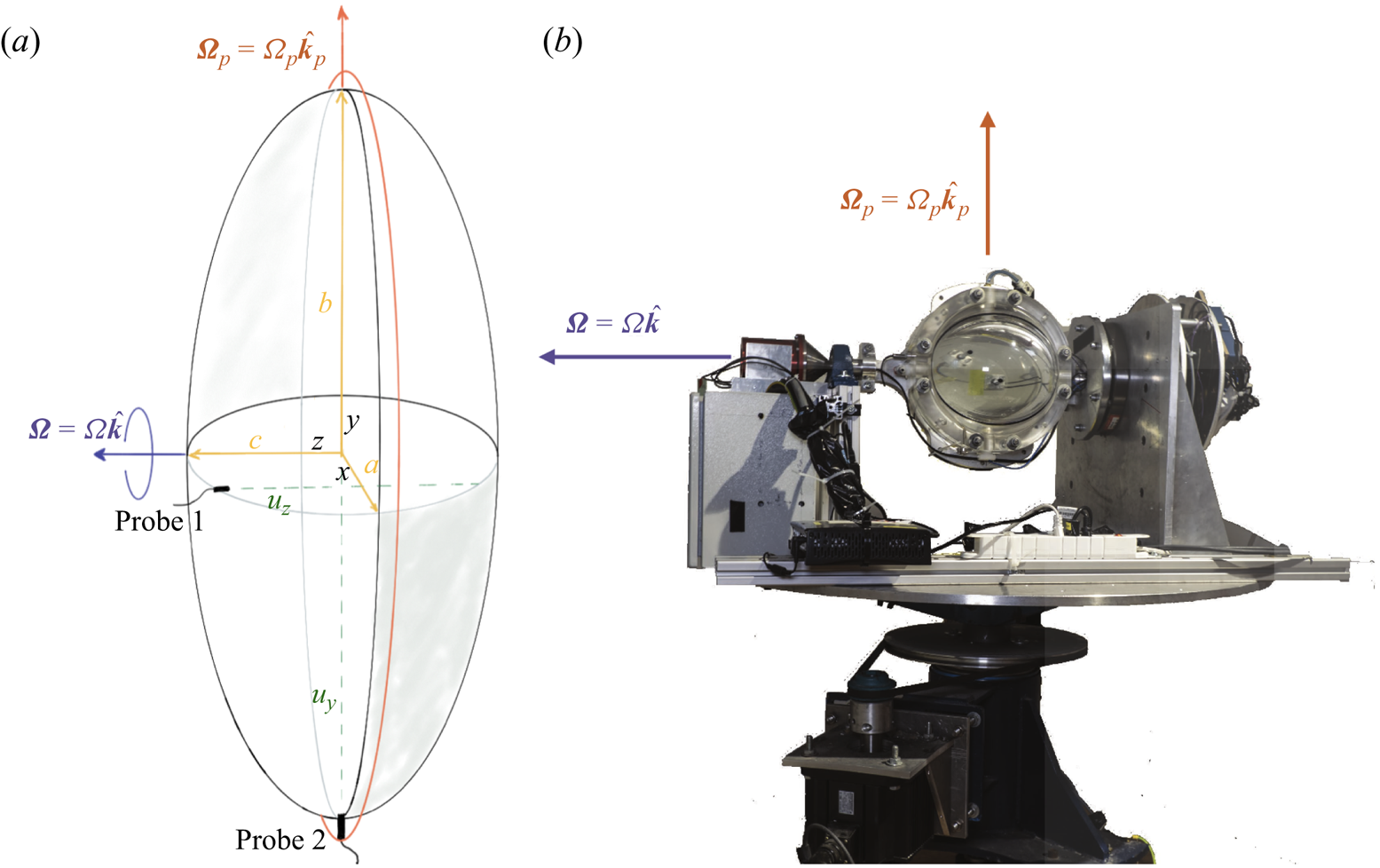
  $\hat {\boldsymbol {k}}_p$, as depicted in figure 1. In this study, the angle between the precession and rotation axis is fixed at $90^\circ$, i.e. $\hat {\boldsymbol {k}_c}\boldsymbol {\cdot }\hat {\boldsymbol {k}_p}=0$. The cavity is filled with an incompressible fluid of constant kinematic viscosity $\nu$. Using $R$ as a length scale and $\varOmega ^{-1}$ as a time scale, the dimensionless equations governing the fluid velocity $\boldsymbol {u}$ and pressure $p$ in the frame of reference co-rotating with the ellipsoid are
 $$\begin{gather} \frac{\partial{\boldsymbol{u}}}{\partial{t}} + \boldsymbol{u} \boldsymbol{\cdot}\boldsymbol{\nabla}\boldsymbol{u} +2\left(\hat{\boldsymbol{k}}+Po\,\hat{\boldsymbol{k}}_p\right)\times\boldsymbol{u} ={-}\boldsymbol{\nabla} p + E\,\nabla^2\boldsymbol{u} - Po \left(\hat{\boldsymbol{k}}_p \times\hat{\boldsymbol{k}}\right) \times \boldsymbol{r}, \end{gather}$$
 $$\begin{gather}\boldsymbol{\nabla}\boldsymbol{\cdot}\boldsymbol{u}=0, \end{gather}$$
subject to the no-slip boundary condition
 \begin{equation} \boldsymbol{u}=0. \end{equation}
In (2.2), we have introduced the two control parameters of the system, the Ekman number and the Poincaré number:
 \begin{equation} E = \frac{\nu}{\varOmega R^2} \quad\text{and} \quad Po=\frac{\varOmega_p}{\varOmega}. \end{equation}
The Ekman number measures the relative importance of viscous force and Coriolis acceleration, and the Poincaré number represents the ratio of the precession to rotation frequencies.
(a) Sketch of the problem: an ellipsoid with the three principal axes  $b>c>a$ is spinning at $\varOmega$ around $c$, which itself is precessing at $\varOmega _p$ around $\hat {\boldsymbol{k}}_p$. A Cartesian coordinate system is placed in such a way that the $z$ axis of the coordinate system is aligned with the mid-axis $c$. We also depict two of the ultrasonic Doppler velocimetry probes: probe 1 is placed off the principal axis and is used to measure the base flow of uniform vorticity; probe 2 is placed along one of the principal axes and is used to measure the flow associated with instabilities. (b) Photograph of the experimental device.
2.2. The base flow of uniform vorticity
In the same vein as previous theoretical studies considering precessing spheroids, Noir & Cébron (Reference Noir and Cébron2013) investigated non-axisymmetric ellipsoids, assuming a leading-order flow of uniform vorticity, without imposing steadiness in any frame of reference. In the frame co-rotating with the ellipsoid, the base flow velocity  $\boldsymbol {U}=(U_x,U_y,U_z)$ is written as
 \begin{equation} \boldsymbol{U} = \boldsymbol{\omega}_f \times \boldsymbol{r} + \boldsymbol{\nabla} \psi, \end{equation}
where  $\boldsymbol {\omega }_f=(\omega _{x},\omega _y,\omega _z)$ denotes the fluid rotation vector, and $\psi$ is a potential field required to satisfy the no-penetration boundary condition at the ellipsoid walls. Noir & Cébron (Reference Noir and Cébron2013) give the following expression for $\psi$:
 \begin{equation} \psi= \omega_x\,\frac{c^2-b^2}{c^2+b^2}\,yz+\omega_y\,\frac{a^2-c^2}{a^2+c^2}\,xz+\omega_z\,\frac{b^2-a^2}{b^2+a^2}\,xy. \end{equation}
Substituting (2.6) into (2.5), the expression of the uniform vorticity velocity can be recast as
 $$\begin{gather} U_x = \omega_y\,\frac{2a^2}{a^2+c^2}\,z - \omega_z\,\frac{2a^2}{a^2+b^2}\,y, \end{gather}$$
 $$\begin{gather}U_y = \omega_z\,\frac{2b^2}{a^2+b^2}\,x - \omega_x\,\frac{2b^2}{c^2+b^2}\,z, \end{gather}$$
 $$\begin{gather}U_z = \omega_x\,\frac{2c^2}{b^2+c^2}\,y - \omega_y\,\frac{2c^2}{a^2+c^2}\,x. \end{gather}$$
Anticipating the rest of the paper, we further define the total fluid rotation as
 \begin{equation} \boldsymbol{\varOmega}_f=\boldsymbol{\omega}_f + \boldsymbol{k}. \end{equation}
As shown by Noir & Cébron (Reference Noir and Cébron2013), taking the curl of the Navier–Stokes equation, and substituting expressions (2.7)–(2.9) for the velocity, yields the following set of ordinary differential equations (ODEs) for the evolution of  $\omega _x$, $\omega _y$ and $\omega _z$:
 \begin{align} \frac{\partial \omega_x}{\partial t}&= \left[\frac{2a^{2}}{a^{2}+c^{2}}-\frac{2a^{2}}{a^{2}+b^{2}}\right]\omega_z\omega_y + Po \sin(t)\,\frac{2a^{2}}{a^{2}+b^{2}}\,\omega_z \nonumber\\ &\quad + \frac{2a^{2}}{a^{2}+c^{2}}\,\omega_y+ Po \sin(t)+\boldsymbol{\mathsf{L}}\boldsymbol{\varGamma}_x, \end{align}
 \begin{align} \frac{\partial \omega_y}{\partial t} &= \left[\frac{2b^{2}}{a^{2}+b^{2}}-\frac{2b^{2}}{b^{2}+c^{2}}\right]\omega_x\omega_z + Po \cos(t)\, \frac{2b^{2}}{a^{2}+b^{2}}\,\omega_z \nonumber\\ &\quad - \frac{2b^{2}}{b^{2}+c^{2}}\,\omega_x+ Po \cos(t)+\boldsymbol{\mathsf{L}}\boldsymbol{\varGamma}_y, \end{align}
 \begin{align} \frac{\partial \omega_z}{\partial t} &= \left[\frac{2c^{2}}{b^{2}+c^{2}}-\frac{2c^{2}}{a^{2}+c^{2}}\right]\omega_x\omega_y - Po \cos(t)\, \frac{2c^{2}}{a^{2}+c^{2}}\,\omega_y \nonumber\\ &\quad - Po \sin (t)\,\frac{2c^{2}}{b^{2}+c^{2}}\,\omega_x +\boldsymbol{\mathsf{L}}\boldsymbol{\varGamma}_z. \end{align}
These equations are complemented by an expression for the viscous term  $\boldsymbol{\mathsf{L}}\boldsymbol{\varGamma}$ as outlined in the Appendix of Noir & Cébron (Reference Noir and Cébron2013):
 \begin{equation} \boldsymbol{\mathsf{L}}\boldsymbol{\varGamma}=\sqrt{E\varOmega}\left( \lambda_r \begin{bmatrix}\varOmega_x\\\varOmega_y\\\varOmega_z-1\end{bmatrix} + \frac{\lambda_i}{\varOmega}\begin{bmatrix}\varOmega_y\\-\varOmega_x\\0\end{bmatrix} +\frac{\varOmega^2-\varOmega_z}{\varOmega^2} \left( \lambda_{sup} -\lambda_{r} \right) \begin{bmatrix}\varOmega_x\\\varOmega_y\\\varOmega_z\end{bmatrix} \right), \end{equation}
where  $\lambda _r$ and $\lambda _i$ denote the real and imaginary parts of the damping of the spin-over mode, and $\lambda _{sup}$ the decay factor of the spin-up. In our preceding paper (Burmann & Noir Reference Burmann and Noir2022), we have validated this model experimentally in the case where multiple solutions and hysteresis cycles exist. Here, we will follow the same procedure to integrate the system of ODEs to calculate the fluid rotation component and compare it to our experimental measurements. We refer the reader to Burmann & Noir (Reference Burmann and Noir2022) for further details on the integration procedure.
2.3. Scaling laws of the onset of the instabilities in spheres and spheroids
So far, there exists no analytical derivation of an instability criterion in non-axisymmetric ellipsoids. Nevertheless, one may gain insight from the scaling laws for the onset of the different parametric and boundary layer instabilities, established in spheres and spheroids.
2.3.1. Ekman boundary layer instability
The onset of instabilities in the Ekman boundary layer is usually characterised by means of a critical local Reynolds number for the Ekman boundary layer:
 \begin{equation} Re_{bl}=\frac{\tilde{U}\delta}{\nu}, \end{equation}
where  $\tilde {U}$ denotes the shear velocity at the top of the Ekman layer, and $\delta =R E_f^{1/2}$ is its respective thickness. Note that we have introduced the fluid Ekman number $E_f=E/\varOmega _f$ based on the total rotation of the fluid $\varOmega _f=|\boldsymbol {\varOmega }_f|$ rather than the rotation of the container. As shown by Noir et al. (Reference Noir, Cardin, Jault and Masson2003), $E_f$ better represents the ratio of viscous to Coriolis forces in a precessing cavity where, at large forcing amplitudes, the fluid and container rotation rates can be significantly different. The shear velocity is estimated from the amplitude of the differential rotation $\omega _f=|\boldsymbol {\omega }_f|$, as $\tilde {U}=\omega _f R$, and the local Reynolds number for the boundary layer becomes
 \begin{equation} Re_{bl}=\frac{\omega_f}{\varOmega_f}\,E_f^{{-}1/2}. \end{equation}
 Apart from some particular asymptotic cases,  $\omega _f$ and $\varOmega _f$ are not known a priori, hence $Re_{bl}$ is a diagnostic quantity.
The first instability in a steady Ekman boundary arises for  $Re_{bl}\sim 55$, in the form of longitudinal rolls tilted with respect to the direction of the base flow (Lilly Reference Lilly1966). Subsequently, the boundary layer becomes turbulent for $Re_{bl}\sim 150$ (Caldwell & Van Atta Reference Caldwell and Van Atta1970; Sous, Sommeria & Boyer Reference Sous, Sommeria and Boyer2013). In the case of precession, the oscillating nature of the Ekman layer yields a shift of the critical value of the Reynolds number. Lacking a theoretical derivation of the critical value of $Re$ for an oscillatory boundary layer, we have to obtain estimates from previous experimental and numerical studies. Typically values reported are $Re_{bl}\sim 70$ for the initial instability in spheroids (Lorenzani & Tilgner Reference Lorenzani and Tilgner2001), and a first thickening of the Ekman layer at the end caps of a precessing cylinder has been observed at $Re_{bl}\sim 100$ in a recent numerical study by Pizzi, Giesecke & Stefani (Reference Pizzi, Giesecke and Stefani2021), but a state of boundary layer turbulence has not been reached. Indeed, the onset of boundary layer turbulence in a oscillatory Ekman layer is shifted towards $Re_{bl}\sim 500$ in numerical simulations using a box model by Buffett (Reference Buffett2021).
2.3.2. Parametric instabilities
Parametric instabilities are excited by a resonant coupling between the base flow and two free inertial modes of the fluid cavity. They have been suggested as the main source of bulk instabilities in spherical and spheroidal fluid cavities subject to precession, libration or tides (see the review by Le Bars, Cébron & Le Gal Reference Le Bars, Cébron and Le Gal2015). Parametric instabilities are characterised by a necessary condition on the resonant frequencies of the free inertial modes given by
 \begin{equation} \varpi_1 \pm \varpi_2 = \varpi_0, \end{equation}
where  $\varpi _1$ and $\varpi _2$ denote the frequencies of the two free inertial modes, and $\varpi _0$ denotes the frequency of a forced inertial mode. Depending on the geometry, there are further conditions on the spatial structure of the involved modes.
As outlined in the Introduction, three mechanisms contribute to the base flow in the precessing cavity: the rotation, the stretching potential field  $\psi$, and the oblique shear layers. Each of those can lead to individual parametric instabilities with a different growth rate. In precessing spheres, only the oblique shear layers associated with the Ekman pumping can contribute to the bulk parametric resonances, through the so-called conical shear instability (CSI) of Lin et al. (Reference Lin, Marti and Noir2015). The onset of this instability is defined by a critical differential rotation between the fluid and the container wall, scaling as
 \begin{equation} \omega_f \propto E^{3/10}. \end{equation}
This instability is not restricted to spherical shells, and can also occur in spheroids (Nobili et al. Reference Nobili, Meunier, Favier and Le Bars2020) or ellipsoids, but there exists no formal derivation for the growth rate of the CSI in tri-axial ellipsoids. Nevertheless, one may still expect the scaling in Ekman number to hold for a tri-axial ellipsoid as well, as we expect that neither the dissipative mechanism nor the inertial waves spawn from the critical latitudes to be affected at leading order by the additional deformation. In contrast, the shape of the container will certainly yield an additional scaling as a function of  $a$,
$a$,  $b$ and $c$, a question not addressed in this study with a fixed geometry. It is thus reasonable to assume that the onset of the CSI in our ellipsoid will remain in the form of (2.18).
In his seminal work, Kerswell (Reference Kerswell1993) showed that two additional mechanisms associated with the potential flow  $\boldsymbol {\nabla }\psi$ can drive parametric resonances. The first mechanism results from the periodic elliptical distortion of the streamlines, and the second one stems from the shear of the planes containing these streamlines due to the tilt of the fluid rotation axis with respect to the figure axis. For the sake of clarity, we will refer to the former as the Kerswell elliptical instability (KEI), and the latter as the Kerswell shear instability (KSI). The onsets of these two instabilities in a spheroid of polar ellipticity $\eta$ are given by
 $$\begin{gather} \omega_f \propto \eta^{{-}1/2} E^{1/4}\quad(\text{KEI}), \end{gather}$$
 $$\begin{gather} \omega_f \propto \eta^{{-}1} E^{1/2}\quad(\text{KSI}). \end{gather}$$
To detect those instabilities in our experiments, we will use the combination of three criteria: the necessary resonant frequency condition (2.17), the sufficient condition of non-vanishing anti-symmetric energy (as defined below in (4.9)), and the direct observations of disorder in the fluid interior.
3. The experimental apparatus and diagnostics
3.1. The experimental set-up
The experimental set-up consists of an acrylic container of ellipsoidal shape with the three semi-major axes  $a = 0.078\ \text {m}$, ${b= 0.125\ \text {m}}$ and ${c = 0.104\ \text {m}}$, and mean radius $R=(abc)^{1/3} = 0.1\ \text {m}$. The container is filled with de-ionised water at room temperature and kinematic viscosity $\nu \sim 1\times 10^{-6}\ \text {m}^2\ \text {s}^{-1}$. The container is set into rotation at $\varOmega$ around its mid-axis $c$, which itself is slowly precessing at $\varOmega _p$ (see figure 1). The precession angle of our experiment is set to $90^\circ$, i.e.
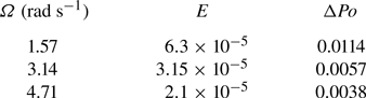
  $\hat {\boldsymbol {k}}_p\boldsymbol {\cdot } \hat {\boldsymbol {k}} =0$ (for a detailed description of the device see Burmann & Noir Reference Burmann and Noir2022). In this study, we perform experiments at three distinct rotation rates, which are listed in table 1 together with the corresponding Ekman number $E$ and minimal increment of the Poincaré number $\Delta Po$.
Rotation rates of the cavity in conducted experiments, together with the respective Ekman number  $E$ and and the minimal increment of the Poincaré number $\Delta Po$.
3.2. Diagnostics
To infer the flow inside our experiment, we make use of both quantitative ultrasonic Doppler velocimetry (UDV) and qualitative visualisation using rheoscopic fluid. For the UDV measurements, we use a DOP4010 system (Signal Processing SA,1073 Savigny, Switzerland), which allows us to measure time-resolved velocity profiles along selected chords in the fluid at spatial resolution 0.5 mm, with typical temporal resolution of the order of 10 Hz. For UDV measurements, the fluid is seeded with 2AP1 Griltex particles of density  $1.02\ {\rm g}\ {\rm cm}^{-3}$, and mixed sizes $50\ \mathrm {\mu }{\rm m}$ (60 % by weight) and
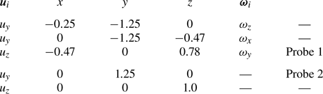
  $80\ \mathrm {\mu }{\rm m}$ (40 % by weight). The positions and orientations of all UDV probes are summarised in table 2.
Position of the UDV probes (centre of the front lens), measured velocity components ( $\boldsymbol {u}_i$) and associated component of the fluid rotation vector ( $\boldsymbol {\omega }_i$). The upper part of the table lists probes that are used to measure the uniform vorticity flow; the lower part of the table lists probes that are used to measure the non-uniform vorticity flow. Probes 1 and 2 are the two probes that are drawn in figure 1. All coordinates are non-dimensional.
For the direct visualisations, we use a home made rheoscopic fluid following the recipe of Borrero-Echeverry, Crowley & Riddick (Reference Borrero-Echeverry, Crowley and Riddick2018). We attach a 1 Watt continuous green laser with a line generator to the rotating ellipsoid. Images are taken with a camera attached to the turntable, i.e. the precession frame.
4. Results
4.1. Base flow of uniform vorticity
Substituting the positions and orientations of the first three probes listed in table 2 into the expressions for the velocity components (2.7)–(2.9), an estimate of  $\omega _x$, $\omega _y$ and $\omega _z$ is readily obtained by averaging the velocity of the off-axis probes along the profile. For example, probe 1 is located at $x=-0.47$ and $y=0$, and measures $U_z$ along $z$ (see also figure 1). The $z$-component of the uniform vorticity flow is given by (2.9): at the location of probe 1, the first summand vanishes, and $U_z$ takes a constant value along the measurement chord, determined only by $\omega _y$, $a$,
$a$,  $c$ and the $x$-coordinate of the probe. Hence for each of the probes located off the figure axis, we compute the mean velocity along the profile and then reconstruct time series of the three components of the fluid rotation vector from (2.7)–(2.9). We then compute the time-averaged differential rotation between the fluid and the container:
 \begin{equation} \left\langle\omega_f \right\rangle_t=\left\langle\sqrt{\omega_x^2+\omega_y^2+\omega_z^2}\right\rangle_t, \end{equation}
where  $\langle \cdot \rangle _t$ denotes the time averaging over a typical window of 100 rotations. Additionally, we define the total rotation rate of the fluid viewed from the precessing frame of the turntable as
 \begin{equation} \left\langle\varOmega_f\right\rangle_t=\left\langle\sqrt{\omega_x^2+\omega_y^2+(\omega_z+1)^2}\right\rangle_t.\end{equation}
Finally, the time-averaged angle of the fluid rotation with respect to the container rotation axis is defined as
 \begin{equation} \langle\theta\rangle_t= \left\langle\arccos \left(\frac{\omega_z+1}{\varOmega_f} \right)\right\rangle_t. \end{equation}
 Figure 2 presents those observables as functions of  $Po$ for a fixed Ekman number $E = 6.3\times 10^{-5}$. We performed two sets of measurements, the first starting from $Po =0.01$ and then increasing $Po$ between subsequent experiments (red, upward triangles), and the second starting from $Po=0.3$ and then decreasing $Po$ (olive, downward triangles). In addition, we present the theoretical prediction obtained by integrating the set of ODEs (2.11)–(2.13). For comparison, we also show in figures 2(d–f) the results of Burmann & Noir (Reference Burmann and Noir2022) when the same container is rotating along its short axis, showing bi-stability of the Poincaré flow. In all plots, the error bars represent the standard deviation of the respective quantity over the entire time series.
Characterisation of the uniform vorticity base flow inside the precessing ellipsoid: (a) differential rotation between fluid and container following (4.1); (b) total fluid rotation viewed from the frame of precession following (4.2); (c) angle between fluid and container rotation axis following (4.3). For comparison, we also show in (d–f) the same quantities when the ellipsoid spins around its shortest axis (Burmann & Noir Reference Burmann and Noir2022). In all plots, we display data from increasing  $Po$ as upward red triangles, and for decreasing $Po$ as downward olive triangles. The error bars are representative of the standard deviation over the entire time series. In all plots, the theoretical predictions from the model of Noir & Cébron (Reference Noir and Cébron2013) are represented as solid black lines.
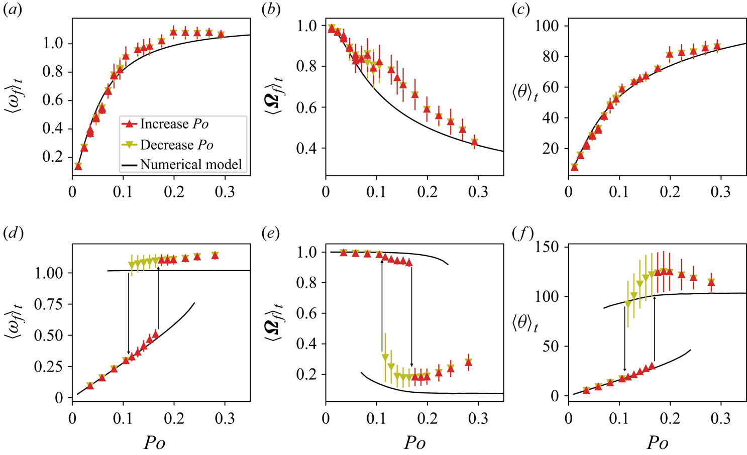
The new results exhibit a very good agreement between the experimental and theoretical estimates for all three quantities at small  $Po$. For $Po>0.1$, some discrepancy is observed, in particular on the total fluid rotation. Yet the model and experiments both show a gradual increase of the differential rotation and a gradual decrease of the total fluid rotation as the tilt of the fluid rotation axis increases with respect to the rotation axis of the container. In contrast with the previous results of Burmann & Noir (Reference Burmann and Noir2022), we do not observe two separate branches of solutions for the uniform vorticity, and consequently no hysteresis cycles between the increasing and decreasing $Po$ experiments. The absence of multiple branches allows for better control of the onset of the instability by continuously increasing the differential rotation, which will be discussed later in this paper.
Our experimental results further validate the theoretical model proposed by Noir & Cébron (Reference Noir and Cébron2013) in a regime not explored in previous experimental studies. We seek to use this model to delineate the regions in the parameter space where multiple or single branches and hysteresis may exist. To characterise the ellipsoids of different axial and equatorial deformations, we follow Vantieghem (Reference Vantieghem2014) and introduce two quantities to characterise the shape of the container:
 \begin{equation} \bar{c} =\frac{c}{\bar{R}}\quad\text{and}\quad\beta = \frac{a^2-b^2}{a^2+b^2}, \end{equation}
where  $\bar {R}$ denotes the mean equatorial radius
 \begin{equation} \bar{R} = \sqrt{\frac{a^2+b^2}{2}}. \end{equation}
Following the same procedure as outlined in § 2.2 of Burmann & Noir (Reference Burmann and Noir2022), we integrate the set of ODEs (2.11)–(2.13) for various combinations of  $\beta$ and $\bar {c}$, keeping the volume of the ellipsoid fixed, and determine the existence of bi-stability in regions of the $(\beta,\bar {c})$ plane. We sample 360 different values of $Po$ in a range from $Po=0.01$ to $Po=0.6$ with resolution ${\sim }0.0016$, and integrate the system of ODEs for 15 spin-up times, starting from 50 random initial conditions ( $\omega _x,\omega _y,\omega _z$). To assess whether bi-stability is present, we compute the mean and standard deviation ( $\sigma$) of the differential rotation $\omega _f$ over the 50 initial conditions at each value of $Po$. Naturally, single branch solutions are characterised by small $\sigma$, while bi-stable solutions are characterised by large standard deviation. To ascertain the bi-stability of each geometry $(\beta,\bar {c})$, we take the maximum standard deviation $\sigma _{max}$ over the whole range of $Po$, and if $\sigma _{max}>0.04$, then the geometry is considered as bi-stable. This threshold value is rather empirical and dictated by the well-documented cases investigated in Burmann & Noir (Reference Burmann and Noir2022). In figure 3, we show maps of $\sigma _{max}$ as functions of $\beta$ and $\bar {c}$, at three different Ekman numbers, $E=10^{-3}$, $6.3\times 10^{-5}$ and $10^{-7}$. The white dots represent those values of $(\beta,\bar {c})$, for which calculations have been performed. We chose the colour scale so that the darker blue level corresponds to $\sigma _{max}<0.04$, for which all initial conditions lead to the same final unique solution.
Bi-stability as a function of deformation: maximum observed standard deviation  $\sigma _{max}$ as a function of $\beta$ and $\bar {c}$ at three different Ekman numbers: (a) $E=1 \times 10^{-3}$, (b) $E=6.3 \times 10^{-5}$ (the same value as in our experiments), and (c) $E=1 \times 10^{-7}$. The colour scale is chosen such that the darkest blue represents cases with no bi-stability, i.e. $\sigma _{max}<0.04$. The present experiment is represented by a red diamond at $(\beta,\bar {c})=(0.44,0.99)$, and the experiment of Burmann & Noir (Reference Burmann and Noir2022) by a red circle at $(\beta,\bar {c})=(0.18,0.68)$. The black horizontal lines denote the critical value of $\bar {c}$ from the bi-stability criterion of Komoda & Goto (Reference Komoda and Goto2019). The directory containing the notebook and data can be accessed at https://www.cambridge.org/S0022112024007742/JFM-Notebooks/files/Figure3.
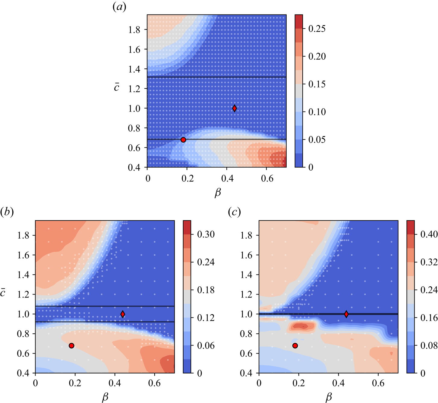
As the Ekman number is increased, the region of single solutions grows, while the region of multiple solutions shrinks, for both prolate ( $\bar {c}>1$) and oblate ( $\bar {c}<1$) ellipsoids. Noticeably, prolate ellipsoids are less prone to bi-stability than oblate spheroids. The two configurations accessible with our experimental device are denoted by red symbols in figure 3. The configuration of the present study (red diamond) plots well within a region of single solutions for all three investigated Ekman numbers. In contrast, the ellipsoid of Burmann & Noir (Reference Burmann and Noir2022) (red circle) is right on the edge of the multiple solution region at the largest Ekman number. We confirm this observation in figure 4, where we display $\langle \omega _f\rangle _t$ as a function of $Po$ for different Ekman numbers down to $E=10^{-10}$. Indeed, the ellipsoid of Burmann & Noir (Reference Burmann and Noir2022) loses bi-stability at $E>10^{-2}$, whereas the configuration studied in the present paper retains a single solution for all Ekman numbers. Furthermore, the curves for $E<10^{-6}$ overlap, indicating that an asymptotic state is reached.
Numerical results for  $\langle \omega _f\rangle _t$ as function of $Po$ at different Ekman numbers, for (a) the ellipsoid of the present study, and (b) the ellipsoid of Burmann & Noir (Reference Burmann and Noir2022). The upward and downward arrows in (b) indicate the branch transitions.

While we can predict the regions of bi-stability numerically, we do not have any analytical criterion for the existence of hysteresis in tri-axial ellipsoids. In the case of spheroids, Komoda & Goto (Reference Komoda and Goto2019) obtained a condition for the existence of a hysteresis cycle given by
 \begin{equation} |\eta| = |\bar{c}-1| > \alpha E^{1/2}, \end{equation}
with  $\alpha \sim 10$. For the three different Ekman numbers investigated here, we display their criteria as black horizontal lines in figure 3. Even though the criteria do not account for the equatorial ellipticity $\beta$, they capture qualitatively the transition to bi-stability for $E=10^{-7}$ and for $E=6.3 \times 10^{-5}$ in the limit of small $\beta$ and up to finite values for $\bar {c}<1$.
4.2. Onset of instabilities
In this subsection, we aim to characterise the onset of instabilities in a precessing ellipsoid and to identify the dominant underlying mechanism. To do so, we combine three different criteria to define the onset of instability: direct visualisation with rheoscopic fluid, anti-symmetric energy, and the frequency spectrum.
4.2.1. Direct visualisations
Figure 5 illustrates shear structures in the bulk obtained with a low concentration of rheoscopic fluid, while figure 6 shows shear in the vicinity of the wall using a saturated solution. Bulk visualisations suggest instabilities for the cases  $Po\gtrsim 0.058$ at $E=6.3\times 10^{-5}$ and $Po\gtrsim 0.047$ at $E=3.1 \times 10^{-5}$. We note in particular the S-shape at $Po=0.058$, typical of parametric instabilities at onset (e.g. Lacaze, Le Gal & Le Dizès Reference Lacaze, Le Gal and Le Dizès2004). From the boundary layer visualisations, it may be argued that near wall structures are already identified at $Po=0.047$ and
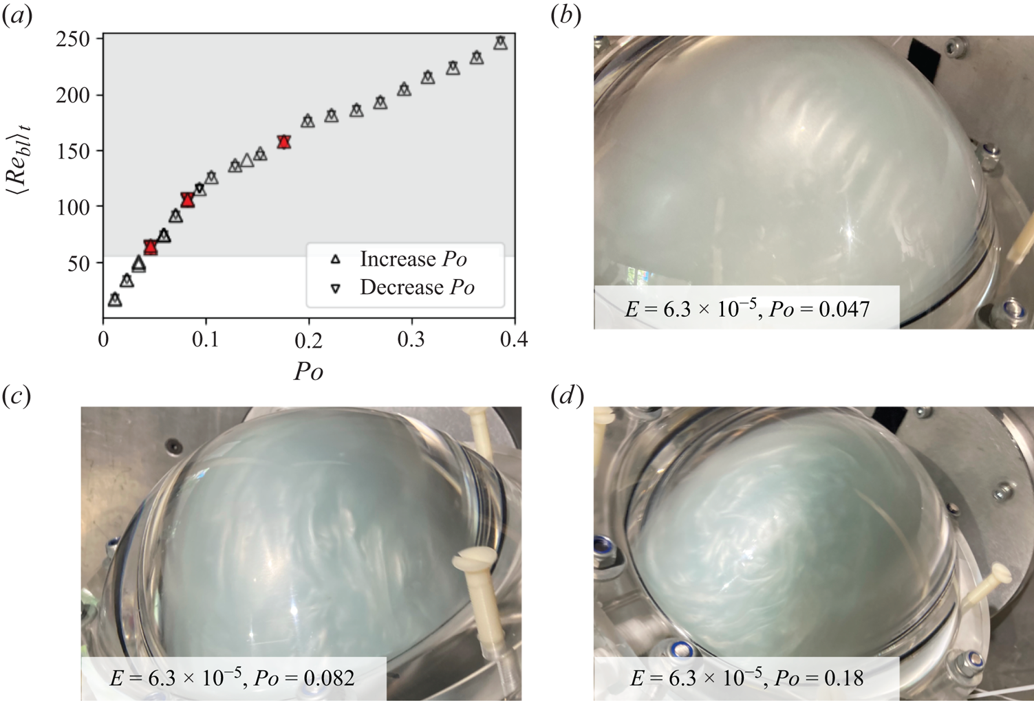
  $E=6.3\times 10^{-5}$, if those are interpreted as the onset of the Ekman layer instabilities. Yet figure 5(b) suggests that they would not have significant influence in the bulk. In figure 6(a) we report the estimated time-averaged $Re_{bl}$ according to (2.16) as a function of $Po$. The points corresponding to the images in figures 6(b–d) are represented with red symbols, and the range of onset values reported in the literature is represented by the grey shaded background starting at $Re_{bl}>55$. However, in precessing cavities, where the Ekman layer is oscillatory, we expect the onset to be shifted towards $Re_{bl}\sim 70\unicode{x2013}100$, as reported in numerical studies using either spheroidal (Lorenzani & Tilgner Reference Lorenzani and Tilgner2001) or cylindrical (Pizzi et al. Reference Pizzi, Giesecke and Stefani2021) geometries. Despite the values for $Re_{bl}$ plotting within the grey range, the values never reach values for boundary layer turbulence, and we suggest that the near-wall shear structures observed in figure 6 may reflect the penetration of the bulk instability impinging in the boundary layer, rather than the development of a boundary layer instability itself. However, given the similar scaling laws for the boundary layer instability (2.16) and the parametric instabilities (2.18)–(2.20), we should not exclude the possibility that both mechanisms could coexist near onset.
Visualisation of the flow using rheoscopic fluid. All pictures are taken with a camera fixed on the turntable, i.e. from the frame of precession. Here, (a,c,e,g)  $E = 3.1\times 10^{-5}$, and (b,d,f,h) $E = 6.3\times 10^{-5}$.

State of the Ekman boundary layer in the experiments. (a) Local Reynolds number  $Re_{bl}$ as a function of $Po$ for increasing and decreasing $Po$ as upward and downward triangles, respectively. (b–d) Visualisations of the boundary layer using high concentrations of rheoscopic fluid. The respective $Re_{bl}$ values of the visualisations are marked in red in (a). The grey shaded area denotes values $Re_{bl}>55$ for which Ekman layer instabilities have been reported previously.
4.2.2. Anti-symmetric energy
The uniform vorticity response of the fluid, including the Ekman pumping, satisfies the symmetry
 \begin{equation} \boldsymbol{U}(-\boldsymbol{r})={-}\boldsymbol{U}(\boldsymbol{r}). \end{equation}
We refer to such flows as symmetric, whereas a flow satisfying
 \begin{equation} \boldsymbol{U}(-\boldsymbol{r})=\boldsymbol{U}(\boldsymbol{r}), \end{equation}
will be called anti-symmetric. Several numerical and experimental studies of precession reported a breaking of this symmetry associated with the onset of instabilities (e.g. Lorenzani & Tilgner Reference Lorenzani and Tilgner2001; Lin et al. Reference Lin, Marti and Noir2015). The growth of an anti-symmetric component of the flow is thus a sufficient, but not necessary, condition to identify the growth of an instability.
Following (2.7)–(2.9), the component of the base flow along the figure axis vanishes, e.g.  $U_{x}=0$ at $(x,0,0)$. Hence a UDV probe measuring velocity profiles along one of the figure axes, such as the exemplary probe 2 in figure 1, will be insensitive to the inviscid part of the base flow. We therefore use such probes to investigate the onset of the instability and calculate the symmetric ( $\boldsymbol {u}_s(\boldsymbol {r},t)$) and anti-symmetric ( $\boldsymbol {u}_a(\boldsymbol {r},t)$) components of the velocity:
 $$\begin{gather} \boldsymbol{u}_a =\frac{\boldsymbol{u}(\boldsymbol{r})+\boldsymbol{u}(-\boldsymbol{r})}{2}, \end{gather}$$
 $$\begin{gather}\boldsymbol{u}_s =\frac{\boldsymbol{u}(\boldsymbol{r})-\boldsymbol{u}(-\boldsymbol{r})}{2}. \end{gather}$$
We then calculate the time-averaged anti-symmetric energy density as
 \begin{equation} \left\langle\mathcal{E}_{a}\right\rangle_t = \left\langle \tfrac{1}{2}\int_L \left| \boldsymbol{u}_a(\boldsymbol{r}) \right|^2{\rm d}l \right\rangle_t. \end{equation}
The results are presented in figure 7 as functions of  $Po$, for three different Ekman numbers. In all experiments, we first observe low values of the anti-symmetric energy for small $Po$, associated with the inherent measurement error at almost vanishing velocities. Past a critical value $Po_c$, the mean anti-symmetric energy increases significantly, which we interpret as the signature of the instability. This is also reflected in a sudden increase of the standard deviation of the anti-symmetric kinetic energy represented by the error bars in figure 7. For the three Ekman numbers investigated, we label all points for which the anti-symmetric energy departs significantly from the low $Po$ values as unstable, and report them as orange symbols in figure 7. Based on these observations, we define the critical value $Po_c$, as the mean value between the last stable point and the first unstable point. The corresponding range in $Po$ is indicated by the grey shaded area in figure 7, and also reported as $\Delta Po_c$ in table 3.
Time-averaged anti-symmetric kinetic energy  $\langle \mathcal {E}_{a}\rangle _t$ measured on the principal axes of the ellipsoid as functions of $Po$ for three investigated Ekman numbers. Stable points are displayed in blue, unstable points in orange, and the error bars are representative of the standard deviation over the entire time series. The grey shaded area represents a region of uncertainty for the onset of instabilities. Here, (a) $E=2.1\times 10^{-5}$, (b) $E=3.1\times 10^{-5}$, and (c) $E=6.3\times 10^{-5}$.

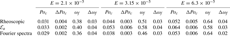
Critical values of  $Po$ determined from the three different criteria together with the corresponding uncertainty range $\Delta Po_c$ and the differential rotation $\omega _f$ obtained from the numerical model.
4.2.3. Frequency spectrum
A classical criterion to detect parametric instability is based on the necessary frequency condition for resonance of (2.17). Using the UDV profiles from the two probes measuring the velocity along the figure axis, we compute the discrete Fourier transform in time, at each location along the profile. We then stack the spectra from all points along the UDV chords, and combine the data sets from the two profiles of  $u_x$ and $u_z$ to increase the signal over noise ratio. Note that the criterion based on the frequency does not require us to separate the symmetric and anti-symmetric parts. In fact, it is even desirable to keep both parts of the velocity to include possible resonances with symmetric modes, otherwise not captured with the anti-symmetric velocity alone.
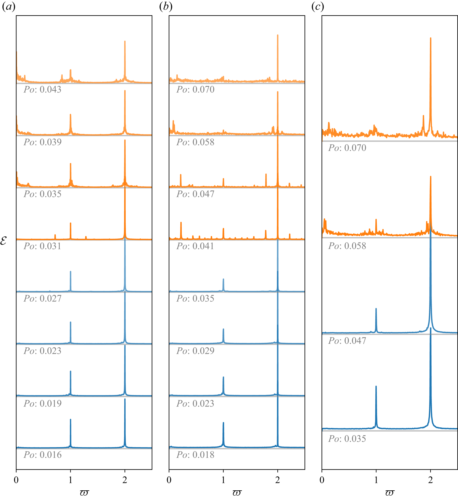
The results are presented in figure 8. At low  $Po$, the spectra exhibit mainly two peaks, at $\varpi =1$ and $\varpi =2$, representing the non-uniform vorticity component of the direct forcing, e.g. the Ekman pumping driven by the base flow and its first harmonics. A typical example of parametric resonances is observed at $Po=0.035$ for $E=2.1\times 10^{-5}$, where two additional peaks arise that satisfy the condition (2.17). At all Ekman numbers, the spectra showing parametric resonances are coloured in orange in figure 8. Again, we define the critical value of $Po_c$ for the onset of instability as the mean value between the last stable and first unstable $Po$, and report the corresponding values in table 3.
Fourier spectra of the non-uniform vorticity flow. All spectra represent a stack of all UDV gates and are normalised by the respective  $Po$ of the measurement. Ekman numbers are (a) $E = 2.1\times 10^{-5}$, (b) $E = 3.15\times 10^{-5}$ and (c) $E = 6.3\times 10^{-5}$.
4.3. Stability diagram
We now combine the criteria of direct visualisations, anti-symmetric energy and resonant frequency conditions to delineate the onset of the instability and tentatively unveil the nature of the underlying mechanism. Rather than presenting the results in terms of  $Po_c$ and $E$, we present them in terms of the differential rotation $\omega _f$ and $E$, which allows us to compare directly with the scaling laws presented in § 2.3. Notice that for the lowest values of $E$, we obtain $\omega _f$ by integrating the ODE system and not from measurements. Since the ODE model shows excellent agreement at the small values of $Po$ considered for the onset of instability, this does not impact our conclusions. The stability diagram including all three criteria is presented in figure 9, where the different symbols represent the different criteria, and the blue and orange colours correspond to stable and unstable flows, respectively. All three criteria are within reasonable agreement, making us confident that we capture correctly the leading-order dynamics of the system. At each Ekman number, we define the onset of the instability as the mean of the critical values of the three independent criteria, and the uncertainties as the maximum of all three; the results are reported as black symbols in figure 9.
Stability diagram in  $E$ and $\omega _f$ for the onset of instabilities in our experimental data. Different symbols represent data from the three criteria: rheoscopic fluid visualisation (squares), anti-symmetric kinetic energy (circles), and Fourier spectra (diamonds). Stable points are in blue, and unstable point in orange. We display the critical differential rotation $\omega _{f,c}$ estimated as the mean value from the three criteria, together with its uncertainty as black symbol (see details in the text). The grey lines represent best fitting scaling laws of the form $\omega _{f,c}\propto a E^{1/2}$ for KSI (dashed), $\omega _{f,c}\propto a E^{1/4}$ for KEI (dotted), and $\omega _{f,c}\propto a E^{3/10}$ for CSI (solid), where $a$ denotes the fitting parameter.

To test which of the CSI, KSI and KEI mechanisms is underlying the onset of the instability, we have reported in figure 9 the best fit for the three possible scalings in Ekman number,  $\omega _{f,c} \propto E^{3/10},\,E^{1/2}, E^{1/4}$. Despite our efforts to combine different diagnoses to probe the onset of the instability, the limited range of Ekman numbers accessible in our study does not allow us to conclude clearly which of the three mechanisms prevails. We thus propose to read our results as follows: if one were to associate the reported onsets to any of the three mechanisms in our geometry, then we may expect the CSI and KEI to dominate at moderate Ekman numbers, while at lower Ekman numbers, the shear instability (KSI) should be dominant.
5. Conclusion
We have investigated the flows inside a non-axisymmetric ellipsoid, rotating around its medium axis and precessing at an angle of  $90^\circ$. Our experimental results for the uniform vorticity base flow are in good agreement with the theoretical model of Noir & Cébron (Reference Noir and Cébron2013). In contrast to an earlier study investigating rotation around the shortest axis of the ellipsoid (Burmann & Noir Reference Burmann and Noir2022), we find a continuous evolution from small to large differential rotation between the fluid and the container. In our experiment, this results in the absence of a hysteresis cycle of the base flow. We then use the good agreement between experimental and theoretical models to systematically investigate bi-stability of the base flow as a function of equatorial and axial deformation in various ellipsoids. At moderate equatorial deformation $\beta <0.2$, the existence of bi-stability is governed mainly by the axial deformation $\bar {c}$, and the hysteresis criterion of Komoda & Goto (Reference Komoda and Goto2019), established from the breakdown of the Busse solution in spheroids (Busse Reference Busse1968; Noir et al. Reference Noir, Cardin, Jault and Masson2003), predicts bi-stability surprisingly well. Meanwhile, decreasing the Ekman number leads to a growing number of ellipsoids showing bi-stable solutions, which is in agreement with the analytical work on bi-stability in precessing spheroids by Cébron (Reference Cébron2015). Unfortunately, our experimental set-up does not allow rotations around the longest axis of the ellipsoid, which would have allowed us to further confirm (or disprove) the numerically established areas of bi-stability: when spinning around its longest axis, our ellipsoid would plot at $(\beta,\bar {c})=(0.28,1.36)$ in figure 3, where bi-stability depends strongly on the value of the Ekman number. Already a moderate, and experimentally realisable, increase of one decade in $E$ should result in a loss of the hysteresis cycle in this configuration. The second part of our study is devoted to the fluid instabilities developing inside the ellipsoid, already at relatively small values of the precession forcing. We establish a stability diagram in the $E\unicode{x2013}\omega _f$ space from three independent measures for the onset of the instability: (1) direct visualisations of the flow in the ellipsoid using rheoscopic fluid; (2) the evolution of the anti-symmetric kinetic energy as a function of $Po$; and (3) Fourier spectra of the non-uniform vorticity flow. In the limited range of Ekman numbers accessible in this study, it is difficult to draw a definitive conclusion, but our interpretation would be that the shear instability (KSI) should prevail at sufficiently low values of $E$ in this geometry, whereas larger values of $E$ remain inconclusive based on our data.
Taking a broader view on precession-driven flows, the emergence of triadic resonances and bi-stability is not restricted to spheroids and ellipsoids, but has also been observed in the case of precessing cylinders (for example, in the study of Herault et al. Reference Herault, Gundrum, Giesecke and Stefani2015). Despite the very similar observations, we would like to emphasise that a hysteresis of turbulence as observed in other geometries (Herault et al. Reference Herault, Gundrum, Giesecke and Stefani2015; Komoda & Goto Reference Komoda and Goto2019) is not necessarily linked to the hysteresis of the uniform vorticity base flow observed in precessing ellipsoids or spheroids (e.g. Cébron Reference Cébron2015). A possibility to investigate the relation between the two phenomena could be experiments at precession angles smaller than  $90^\circ$, where the amplitude of the base flow is expected to be weaker, hence less prone to instability. Unfortunately, this is beyond the capabilities of our present experimental device. The limitation in the range of accessible Ekman numbers is a general problem of present-day precession experiments, and it seems clear to us that a significant step towards lower Ekman numbers is necessary to make further progress on the topic of precession-driven flows in non-spherical containers. Fortunately, ongoing experimental projects – e.g. the DRESDYN liquid sodium precessing cylindrical dynamo (Stefani et al. Reference Stefani, Albrecht, Gerbeth, Giesecke, Gundrum, Herault, Nore and Steglich2015) and the recently developed rapidly rotating device at the Key Laboratory of Planetary Sciences of Professor Dali Kong – will provide promising opportunities to study rotating dynamics at lower Ekman numbers.
To allow a fine tuning of the onset of instabilities in low Ekman experiments, one should choose the geometry such that the differential rotation between the fluid and the cavity evolves continuously as in this study, i.e. without hysteresis. In the case of tri-axial ellipsoids, such parameters can be determined using the model of uniform vorticity as in our figure 3. A typical range of deformation could be  $1<\bar {c}<1.4$ and $0.4<\beta <0.6$, allowing us to also investigate the scaling of the onset with the geometry.
Also, numerical simulations using no-slip boundary conditions in deformed spheroids and ellipsoids will not be capable of reaching the desired range of Ekman numbers in the near future. An alternative approach would be to study developing instabilities numerically using free-slip boundary conditions, following the recent suggestion of Vidal & Cébron (Reference Vidal and Cébron2023).
Supplementary material
Computational notebook files are available as supplementary material at https://doi.org/10.1017/jfm.2024.774 and online at https://www.cambridge.org/S0022112024007742/JFM-Notebooks.
Acknowledgements
Numerical simulations were performed on the ETH Zürich Euler cluster. We thank four reviewers for their comments on the manuscript.
Funding
This research is supported by funding from the European Research Council (ERC) under the European Union's Horizon 2020 research and innovation programme (grant agreement no. 833848, UEMHP project). The experimental device was built with the support of SNF grant 200021_140708 and ETH grant ETH-04 22-1.
Declaration of interests
The authors report no conflict of interest.
Appendix. Examples of full time series for the time-averaged quantities of figure 2
In figure 10, we display the time evolution of the same quantities that are displayed as temporal averages in figure 2, i.e. the differential rotation between fluid and container (figure 10a), the total fluid rotation viewed from the frame of precession (figure 10b), and the angle between fluid and container rotation axis (figure 10c). For each observable, we show an illustrative example at small forcing amplitude ( $Po=0.04$) and one at large forcing ( $Po=0.22$), representative of a flow regime with developed instabilities. All time series cover approximately 100 rotations of the ellipsoid, which is the same range used for the temporal averaging in figure 2. For a detailed view on the time evolution of $\omega _x$, $\omega _y$ and $\omega _z$ we refer the reader to the similar figure 13 of our preceding paper (Burmann & Noir Reference Burmann and Noir2022).
Examples of the time evolutions of (a) the differential rotation between fluid and container, (b) the total fluid rotation viewed from the frame of precession, and (c) the angle between fluid and container rotation axis. The displayed time series is the same that is used to calculate the temporal averages displayed in figure 2 and covers 100 rotations of the ellipsoid. The Ekman number is  $E = 6.3\times 10^{-5}$.


 Open access