


1. Introduction
In 1949, Onsager conjectured that for rough enough velocity fields, energy dissipation could arise without the help of viscosity (Onsager Reference Onsager1949; Eyink & Sreenivasan Reference Eyink and Sreenivasan2006). This conjecture was proven by Isett (Reference Isett2018), who used convex integration methods introduced by De Lellis & Szekelyhidi (Reference De Lellis and Szekelyhidi2013, Reference De Lellis and Szekelyhidi2014, Reference De Lellis and Szekelyhidi2015) and the concept of Mikado flow (Daneri & Szekelyhidi Reference Daneri and Szekelyhidi2017) to prove the existence of weak solutions of Euler equations, that do not conserve energy. Conversely, Onsager also conjectured that non-viscous dissipation would not happen for velocity fields that are  $h$-Hölder continuous with the Hölder exponent $h>1/3$. This conjecture was first proven by Constantin & Titi (Reference Constantin and Titi1994), while a simple and elegant proof was later provided by Duchon & Robert (Reference Duchon and Robert2000), using the energy balance equation for weak solutions of the three-dimensional (3-D) incompressible Navier–Stokes equations (INSE)
 \begin{equation} \partial_t \frac {u_i^2} 2 + \partial_j \left[u_j\left(\frac {u_i^2} 2 + p\right)\right]=\nu \varDelta \frac {u_i^2} 2-\nu \partial_j u_i \partial_j u_i+ D(\boldsymbol{u}). \end{equation}
 In this equation,  $\boldsymbol {u}$ is a weak solution of the 3-D INSE, and the derivatives should therefore be understood in the sense of distributions. This energy balance is very similar to that of ordinary 3-D INSE, except for an additional energy dissipation term $D(\boldsymbol {u})$ stemming from the lack of regularity of the velocity field. The parameter $D(\boldsymbol {u})$ is defined as follows:
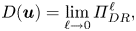 \begin{equation} D(\boldsymbol{u})=\lim_{\ell \rightarrow 0} \varPi_{DR}^\ell, \end{equation}
where  $\Pi ^\ell _{DR}$ originates from the nonlinear (inertial) terms of the 3-D INSE
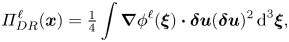 \begin{equation} \varPi_{DR}^\ell(\boldsymbol{x})=\tfrac{1}{4}\int \boldsymbol{\nabla} \phi^\ell ({\boldsymbol{\xi}})\boldsymbol{\cdot} \boldsymbol{\delta} {\boldsymbol{u}} (\boldsymbol{\delta} {\boldsymbol{u}})^2\,\textrm{d}^3\boldsymbol{\xi}, \end{equation}
where  $\phi ^\ell$ is a smooth filtering function and $\boldsymbol {\delta } \boldsymbol {u}$ is the velocity increment, depending implicitly on $\boldsymbol {x}$ and $\boldsymbol {\xi }$: $\boldsymbol {\delta }\boldsymbol {u}(\boldsymbol {x}, \boldsymbol {\xi })={\boldsymbol {u}}(\boldsymbol {x}+\boldsymbol {\xi })- {\boldsymbol {u}}(\boldsymbol {x})$.
Duchon and Robert proposed considering as physically relevant only those solutions for which  $D(\boldsymbol {u})\geqslant 0$, which they call ‘dissipative solutions’, $D(\boldsymbol {u})$ being the ‘inertial dissipation’. They showed that the weak solutions exhibited by Leray (Reference Leray1934) were dissipative solutions; however, they did not exhibit any solution for which $D(\boldsymbol {u})\neq 0$. A balance equation similar to (1.1) holds if $\nu =0$, i.e. in the case of the 3-D incompressible Euler equations. Duchon and Robert also showed that a solution to the 3-D incompressible Euler equations that is the strong limit of a sequence of dissipative weak solutions to the Navier–Stokes equations would be a dissipative solution ( $D(\boldsymbol {u})\geqslant 0$). They further proved that, in the case where $\nu =0$, $D(\boldsymbol {u})=0$ if the velocity field is $h$-Hölder continuous with $h>1/3$ (in particular if the velocity field is regular, i.e. if $h=1$), thus proving Onsager's conjecture. If $h\leqslant 1/3$, $D(\boldsymbol {u})$ may well be non-zero: additional dissipation would then arise from the roughness of the velocity field. This can be understood from the definition of $h$-Hölder continuity since then $|\boldsymbol {\delta } {\boldsymbol {u}}| =O({|\xi }|^h)$ and $\varPi _{DR}^\ell =O( \ell ^{3h-1})$. If $h\leqslant 1/3$, $\Pi ^\ell _{DR}$ does not tend to 0 when $\ell$ tends to 0. On the other hand, if $h=1$, then $D(\boldsymbol {u})= 0$: therefore, if $D(\boldsymbol {u})> 0$, the velocity field is necessarily singular.
What then is the relevance of the above considerations towards a real velocity field? Real flows obey the incompressible Navier–Stokes equations under at least two conditions: (C1) the smallest scales are larger than the mean free path; (C2) the velocity is smaller than the speed of sound, resulting in  $Ma=u/c_s\ll 1$. At the location of a mathematical singularity of the Navier–Stokes equations, the velocity field would extend over arbitrarily small scales, becoming infinite (arbitrarily large) as the scale decreases (Constantin Reference Constantin2008). Therefore, conditions C1 and C2 would not apply anymore and additional physics would come into play, presumably hindering the growth of any mathematical singularity. For instance, one can speculate that the growth of a singularity would generate compressible effects with the associated dissipation mechanism, replacing the inertial dissipation that might have taken place in the incompressible solution by shocks.
To understand the general nature of dissipation processes in incompressible fluids, it is therefore of interest to investigate in more detail what is happening in an experimental flow at places where  $\varPi _{DR}^\ell$ is very large at very small scales (of the order of the Kolmogorov scale): such places may be prints of inertial dissipation occurring in a mathematical solution to the 3-D INSE, which would be replaced, in a real flow, by physical phenomena not included in those equations. Therefore, we study the topology of the velocity field around these events to try to understand how they form. Such a work was initiated in Saw et al. (Reference Saw, Kuzzay, Faranda, Guittonneau, Daviaud, Wiertel-Gasquet, Padilla and Dubrulle2016), where extreme events of a 2-D version of $\Pi ^\ell _{DR}$ are studied in two-dimensional three component (2D-3C) velocity fields measured by stereoscopic particle image velocimetry. Four kinds of structures had been observed, but it was not possible to know whether they were different structures or different cross-sections, possibly observed at different times, of a single one. The use of tomographic particle image velocimetry (TPIV) now allows us to perform three-dimensional three component (3D-3C) measurements of the velocity field and therefore to analyse the full 3-D structure of the detected events.
The article is organized as follows: the experimental set-up is detailed in § 2. The statistics of the quantity underlying the detection criterion as well as the intensity of the detected events are reported in § 3. The structure of the velocity field around the detected events is then characterized with the velocity gradient tensor (VGT) invariants method in § 4 and by direct observations in § 5. The results are then discussed in § 6 before a conclusion is drawn in § 7.
2. Experimental set-up
The velocity fields are measured at the centre of a von Kármán flow, as shown on figure 1(a). Such an area corresponds to the location where the turbulence is the most homogeneous and isotropic, even though it is not rigorously perfectly homogeneous and isotropic (see e.g. Ouellette et al. Reference Ouellette, Xu, Bourgoin and Bodenschatz2006). Previous measurements of spectra, local energy transfer, dissipation or structure functions Debue et al. (Reference Debue, Kuzzay, Saw, Daviaud, Dubrulle, Canet, Rossetto and Wschebor2018a,Reference Debue, Shukla, Kuzzay, Faranda, Saw, Daviaud and Dubrulleb) in that area were found to be in agreement with results from direct numerical simulation of homogeneous isotropic turbulence, and exhibit universality (Geneste et al. Reference Geneste, Faller, Nguyen, Shukla, Laval, Daviaud, Saw and Dubrulle2019). Therefore, we expect the results described in the present paper to be fairly general.
Experimental set-up. (a) Perspective view of the von Kármán flow geometry. The green area at the centre is the measurement volume. (b) Top view of the whole set-up.
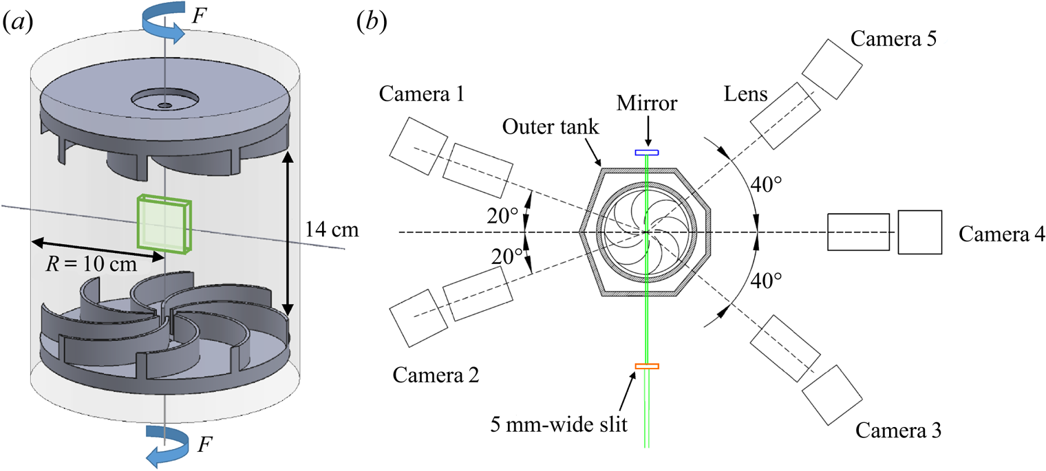
This flow is generated by two counter-rotating impellers in a cylinder whose radius is  $R=10$ cm. The impellers have eight curvated 2 cm high blades, their diameter is 9.25 cm and the distance between the blades is 14 cm. They rotate at the same frequency $F$, in the direction such that the concave side of the blades pushes the fluid. The resulting flow is characterized by a Reynolds number $Re$ based on the impeller rotation frequency $F$, the cylinder radius $R$ and the fluid viscosity $\nu$
$\nu$
 \begin{equation} Re=\frac{2{\rm \pi} R^2 F}\nu. \end{equation}
In this article, the fluid is water at  $20\,^{\circ }\textrm {C}$, and $\nu =10^{-6}\ \textrm {m}^2\ \textrm {s}^{-1}$. The temperature of the fluid is kept constant by means of a cooling system and the impeller rotation frequency is monitored by SCAIME torquemeters; it varies by less than 1 %. For $Re>6000$, the flow is fully turbulent (Ravelet, Chiffaudel & Daviaud Reference Ravelet, Chiffaudel and Daviaud2008). The average flow is then made of two counter-rotating cells; at the centre (i.e. at the intersection of the equatorial plane and of a meridian plane), there is a strong shear but the average velocity is very small. At large Reynolds numbers, the dimensionless root-mean-square (r.m.s.) of the velocity fluctuations is independent of the Reynolds number; the r.m.s. of the fluctuations along the $x$ and $z$ axes is approximately $V/3$ and the r.m.s. of the fluctuations along the $z$ axis is approximately $V/5$, with $V=2{\rm \pi} RF$ the typical large scale velocity. The global average dissipation rate $\epsilon$ can be measured with the torquemeters; its dimensionless value $\epsilon ^*=\epsilon /(2{\rm \pi} F)^3R^2)$ is also independent of $Re$ in the limit of large Reynolds numbers, it is equal to 4.8 $\times 10^{-2}$ in this limit.
The size of the velocity field is  $5\ \textrm {cm}\times 3.5\ \textrm {cm}\times 0.67\ \textrm {cm}$. It is measured by TPIV. Five Imager sCMOS cameras are placed in the same equatorial plane and acquire pictures with different viewing angles, as shown on figure 1(b). They are equipped with Zeiss Milvus 2 lenses mounted on Lavision Scheimpflugs; the numerical aperture is $f_{\#}=11$ and the focal length is 100 mm. The diffraction spot is then 2.8 pixels wide and the depth of field is 7 mm. An outer tank with flat faces and filled with water allows for the reduction of optical distortions due to the interface between air and water. The particles are glass hollow spheres of $10\ \mathrm {\mu }\textrm {m}$ diameter; they are lit by a Solo II PIV laser. A mirror is used so that the laser beam crosses the measurement volume twice; thus, all cameras are both in forward and backward scattering with respect to the incident or the reflected beam and the intensity differences between cameras are reduced. The calibration consists in a first guess realized with a 3-D 2-level calibration plate, and is then refined by a volume self-calibration (Wieneke Reference Wieneke2008) until reaching a disparity lower than 0.2 pixel. The image processing consists in a subtraction of the time average of the camera images. The volume reconstruction consists in four multiplicative algebraic reconstruction technique (a.k.a. MART) iterations (Elsinga et al. Reference Elsinga, Scarano, Wieneke and Van Oudheusden2006); the ghost ratio is smaller than 10 % and the normalized intensity variance larger than 35. The velocity fields are then obtained by a 4-step multi-pass volume correlation with window shifting and deformation; Gaussian interrogation volumes are used, they overlap at 75 %. The final interrogation volume size is 80 pixels, or 1.4 mm in the measurement volume. The space step is thus ${\textrm {d}\kern0.09em x}=0.35\ \mathrm {mm}$, and there are approximately $150\times 100\times 20$ velocity vectors. All the TPIV steps are performed with Davis software of LaVision company.
Varying the impeller rotation frequency  $F$ allows us to modify the Reynolds number of the flow $Re$, and thus the Kolmogorov scale $\eta =R(Re^3\epsilon ^*)^{-1/4}$. With a constant TPIV resolution, we can thus probe different scale ranges, from the inertial range to the dissipative one: indeed, ${\textrm {d}\kern0.09em x}$ being constant, ${\textrm{d}\kern0.09em x}/\eta$ is increasing with
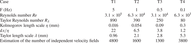
  $Re$. We considered four cases, whose characteristics are summarized in table 1: cases T1 and T2 allow us to probe the inertial range of scales, case T3 the transition range between the inertial and the dissipative ranges and case T4 allows us to probe the dissipative range. In this latter case, as the dissipative scales are resolved, it is possible to estimate the uncertainty on the velocity based on the r.m.s. of the velocity divergence (Atkinson et al. Reference Atkinson, Coudert, Foucaut, Stanislas and Soria2011); we found an uncertainty of 0.3 pixel. In this work, we look for rare events; thus, a large number of uncorrelated velocity fields should be acquired. In our case, we accumulated in each case approximately 40 000 correlated frames, resulting in approximately 10 times less uncorrelated fields; the last line of table 1 gives an estimation of the number of independent velocity fields in each case, depending on the acquisition frequency.
Parameters of the four different experimental cases.
PIV is a measurement method with a finite resolution: indeed, a velocity field measured by PIV can be seen as the real velocity field averaged over the interrogation volume. Therefore, PIV has a filtering effect, with a filter 3 dB cutoff wavenumber well approximated by  $k_{PIV}=2.8/X$ where $X$ is the interrogation volume size (Foucaut, Carlier & Stanislas Reference Foucaut, Carlier and Stanislas2004). The parameter $\Pi ^\ell _{DR}$ can also be seen as a filtered quantity, whose filter is $\phi ^\ell$. In this work, we use $\phi ^\ell (\boldsymbol {x}) \propto \exp ({-30 \boldsymbol {x}^2/(2\ell ^2)})$. As a consequence, computing $\Pi ^\ell _{DR}$ for velocity fields measured by PIV leads to a double filtering. It must then be ensured that the second filter ( $\phi ^\ell$) does not filter less than the first one (the PIV filter). This is ensured if the 3 dB cutoff wavenumber of $\phi ^\ell$ is smaller than $k_c$, i.e. if $\sqrt {30 \ln (2)}/\ell \leqslant k_{PIV}$. In the physical space, the corresponding relevant scales are $\ell _c={\rm \pi} \ell /\sqrt {30 \ln (2)}$ and ${\rm \pi} /k_{PIV}\approx X$: therefore, the double filtering is meaningful if $\ell _c \geqslant X$. In the following, we will mainly use $\ell _c$ as it can be directly compared to $X$; it should always be understood as $\ell _c(\ell )$. According to the ultraviolet locality principle (Eyink Reference Eyink2007–2008), computing $\Pi ^\ell _{DR}$ on an already-filtered velocity field is meaningful as long as $\ell _c/X$ is large enough (and as long as the local Hölder exponent is larger than 0): indeed, the contribution to $\Pi ^\ell _{DR}$ is mainly due to neighbouring scales; therefore, too small scales can be ignored. In this paper, we present results obtained for $\ell _c=1.7X$. Such size is a compromise between constraints inherent to TPIV and constraints to allow physical behaviours' identification.
3. Statistics of  $\Pi ^\ell _{DR}$ with respect to scales and intensity of the extreme events

Our experimental set-up allows us to collect a large number of velocity fields in order to have a statistically relevant sample and thus to observe very strong events. In this section, we report the behaviour of the space–time average and of the probability distribution function (p.d.f.) of  $\Pi ^\ell _{DR}$ before giving the intensity of the extreme events of $\Pi ^\ell _{DR}$ studied in this article.
Figure 2 shows the space–time average of  $\Pi ^\ell _{DR}$ and $\mathscr {D}^\ell _{\nu }$ at four values of $\ell _c/\eta$, each one obtained with one of the cases T1 to T4. $\mathscr {D}^\ell _{\nu }$ is defined as follows:
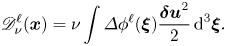 \begin{equation} \mathscr{D}_\nu^\ell (\boldsymbol{x})= \nu \int \varDelta\phi^\ell( \boldsymbol{\xi}) \frac{{\boldsymbol{\delta} \boldsymbol{u}}^2} 2\,\textrm{d}^3 \boldsymbol{\xi} .\end{equation}
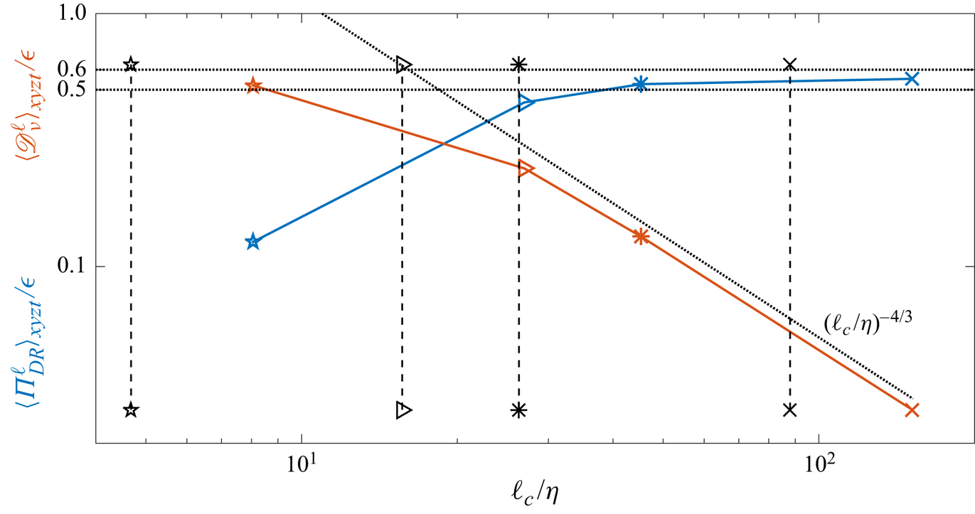
Space–time average of  $\Pi ^\ell _{DR}$ (blue) and $\mathscr {D}^\ell _{\nu }$ (red) with respect to scales. The vertical dashed lines correspond to the interrogation window size (divided by $\eta$). Pentagons: $\ell _c/\eta =8$ (obtained with case T4), triangles: $\ell _c/\eta =27$ (obtained with case T3), stars: $\ell _c/\eta =45$ (obtained with case T2), crosses: $\ell _c/\eta =150$ (obtained with case T1). The dotted line corresponds to the scaling $(\ell _c/\eta )^{-4/3}$.
It measures the viscous dissipation, and is used here rather than the usual  $\nu {\boldsymbol {\nabla }}{\boldsymbol {u}}^\ell :{\boldsymbol {\nabla }}{\boldsymbol {u}}^\ell$ because it appears in the so-called weak Kármán–Howarth–Monin equation (Dubrulle Reference Dubrulle2019) along with $\Pi ^\ell _{DR}$.
Integrals involving the velocity increments can be seen as convolution products of the velocity field with a derivative of the filtering function (first derivative for  $\Pi ^\ell _{DR}$, second derivative for $\mathscr {D}^\ell _{\nu }$). They are therefore first computed in the Fourier space as a scalar product of the Fourier transform of the velocity field and of the Fourier transform of the chosen derivative of the filtering function. The convolution product in the real space is then obtained by Fourier transforming the scalar product obtained in the Fourier space. As experimental velocity fields are discrete and of finite dimensions, not all scales can be investigated but only scales approximately between the space step and the interrogation volume size. The lower and upper scales probed are discussed in more detail in Debue (Reference Debue2019).
It can be shown that the limit of  $\mathscr {D}^\ell _{\nu }$ is the same as the limit of $\nu \boldsymbol{\nabla}\boldsymbol{u}^{\ell}: \boldsymbol{\nabla}\boldsymbol{u}^\ell$,
 \begin{equation} \lim_{\ell \rightarrow 0}\mathscr{D}_\nu^\ell =\nu \partial_j u_i \partial_j u_i. \end{equation}
 As expected,  $\Pi ^\ell _{DR}$ increases and $\mathscr {D}^\ell _{\nu }$ decreases with $\ell _c/\eta$; in the dissipative range, the viscous effects ( $\mathscr {D}^\ell _{\nu }$) dominate the inertial effects ( $\Pi ^\ell _{DR}$) whereas it is the contrary in the inertial range. In the inertial range, both $\Pi ^\ell _{DR}$ and $\mathscr {D}^\ell _{\nu }$ seem to follow the Kolmogorov scalings: saturation of $\Pi ^\ell _{DR}$ and decrease of $\mathscr {D}^\ell _{\nu }$ as $\ell ^{-4/3}$. This average behaviour supports the ability of our multi-scale analysis method to probe different scale ranges.
However, the p.d.f.s in figure 3 show that  $\Pi ^\ell _{DR}$ and $\mathscr {D}^\ell _{\nu }$ do not have similar behaviours: whereas $\mathscr {D}^\ell _{\nu }$ has almost log-normal p.d.f.s and scale-invariant centred-reduced p.d.f.s, the p.d.f.s of $\Pi ^\ell _{DR}$ have wide tails; also, the centred-reduced p.d.f.s of $\Pi ^\ell _{DR}$ are more skewed and have larger positive tails in the dissipative range. Note that the saturation of the p.d.f.s of $\mathscr {D}^\ell _{\nu }$ at low values is most probably spurious and due to the computation of this term. Whereas $\mathscr {D}^\ell _{\nu }$ takes only positive values, $\Pi ^\ell _{DR}$ also has negative values, but its p.d.f.s are skewed towards positive values, and this skewness is stronger in the dissipative range.
Probability density functions of  ${\varPi }_{DR}^\ell$ and of the viscous dissipation $\mathscr {D}_\nu ^\ell$ for cases T1 to T4. The vertical axes are in logarithmic coordinates and the horizontal axes in linear coordinates, except for (b), where it is in logarithmic coordinates. Blue, $\ell _c/\eta =8$ (case T4); red, $\ell _c/\eta =27$ (case T3); orange, $\ell _c/\eta =45$ (case T2); purple, $\ell _c/\eta =150$ (case T1). (a) The p.d.f. of ${\varPi }_{DR}^\ell$ normalized by the global dissipation rate $\epsilon$ (computed from torque measurements). (b) The p.d.f. of $\mathscr {D}_{\nu }^\ell$ normalized by the global dissipation rate $\epsilon$. (c) Centred-reduced p.d.f. of ${\varPi }_{DR}^\ell$. (d) Centred-reduced p.d.f. of $\mathscr {D}_{\nu }^\ell$.
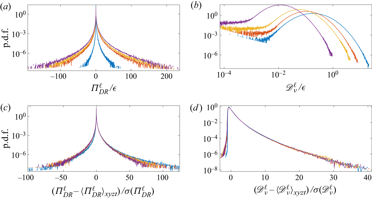
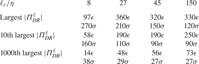
Table 2 gives the values of the 10th and 1000th largest events of  $|\varPi _{DR}^\ell |$ at different values of $\ell _c/\eta$, in terms of $\epsilon$ and of $\sigma$, the standard deviation of the distribution of $\Pi ^\ell _{DR}$. In § 4, the structure of the velocity field at the 1000 strongest events of $|\varPi _{DR}^\ell |$ is analysed with the VGT method and in § 5, the structure of the velocity field around the 10 strongest events only is analysed by direct observation. Even if $\Pi ^\ell _{DR}$ takes smaller values on average in the dissipative range, it can still reach very large values, almost equal to $100\epsilon$, i.e. 200 times the average $\mathscr {D}^\ell _{\nu }$ at the same scale, or 270 times the standard deviation of the p.d.f. of $\varPi _{DR}^\ell$. Interpreting $\Pi ^\ell _{DR}$ as an energy inter-scale transfer rate towards smaller scales, this strongly suggests that there is not a unique dissipative scale, which would be the smallest flow scale, as smaller scales are necessary to dissipate such large transfer at this value of $\ell _c$. This is in agreement with the phenomenological interpretation of the multifractal model (Paladin & Vulpiani Reference Paladin and Vulpiani1987), which suggests that there is a finite range of dissipative scales, which depend on the local smoothness of the velocity field. In the inertial range, the extremes of $\Pi ^\ell _{DR}$ take larger values in terms of $\epsilon$ than in the dissipative range, but these extremes are smaller in terms of standard deviations. This is in agreement with the behaviour of the raw and centred-reduced p.d.f.s.
Values of the 10th and 1000th largest events of  $|\varPi _{DR}^\ell |$ at different values of $\ell _c/\eta$; ‘ $x\epsilon$’ means that the value is equal to $x$ times the global average dissipation rate measured by torquemeters, ‘ $x \sigma$’ means that the value is equal to the space–time average of $\Pi ^\ell _{DR}$ plus $x$ times the (space–time) standard deviation of $\Pi ^\ell _{DR}$.
4. Characterization using the VGT invariants
We first characterize the extreme events of  $\Pi ^\ell _{DR}$ by computing the invariants of the VGT which capture the local topology of the flow. The average behaviour of $\Pi ^\ell _{DR}$ and $\mathscr {D}^\ell _{\nu }$ with respect to the topology can thus be studied, and the distribution of the topology in the whole flow and among the extreme events of $\Pi ^\ell _{DR}$ can be compared.
According to Chong & Perry (Reference Chong, Perry and Cantwell1990), the local topology of a 3-D regular-enough velocity field can be characterized by the invariants of the VGT  $\boldsymbol {\nabla }\boldsymbol {u}$ at the studied point. Let us call $Q=-\textrm {tr}((\boldsymbol {\nabla }\boldsymbol {u})^2)/2$ the second invariant, and $R=-\textrm {det}(\boldsymbol {\nabla }\boldsymbol {u})$ the third invariant of the VGT. For a 3-D incompressible flow, the first VGT invariant, which is $\textrm {tr}(\boldsymbol {\nabla }\boldsymbol {u})$, is zero everywhere as the flow is divergence free; therefore, the sum of the VGT eigenvalues is 0 and there are only four possible configurations or topologies, based on the two following criteria: (i) either there are only real eigenvalues (for $27R^2+4Q^3<0$), or one real and two complex-conjugate eigenvalues ( $27R^2+4Q^3>0$) and (ii) either two eigenvalues have a positive real part (for $R>0$) or only one eigenvalue has a positive real part ( $R<0$), the remaining eigenvalue(s) having a negative real part. The four topologies are:
(i) The ‘filament’ (
$F$), when $27R^2+4Q^3<0$ and $R<0$. The fluid is compressed in two directions and stretched in the third one.(ii) The ‘sheet’ (
$S$), when $27R^2+4Q^3<0$ but $R>0$. The fluid is compressed in one direction and stretched in the two others.(iii) The ‘vortex stretching’, or stable focus/stretching, when
$27R^2+4Q^3>0$ and $R<0$. In one plane, the motion of the fluid is a converging spiral; in the remaining direction the fluid is stretched.(iv) The ‘vortex compressing’, or unstable focus/compressing, when
$27R^2+4Q^3>0$ but $R>0$. The fluid is compressed in one direction; in the plane containing the two other directions, its motion is a diverging spiral.


In this work, we compute the VGT on an experimental velocity field which is smoothed at the resolution scale by the measurement method. Therefore, the velocity field is regular and applying the VGT invariant method is meaningful. The obtained topology is the topology of the flow ‘at the resolution scale’.
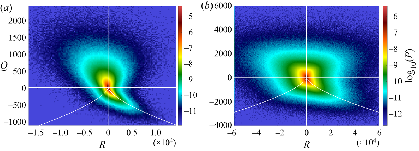
The distribution of the four topologies in the flow can be easily obtained by computing the VGT and its invariants everywhere and forming the joint p.d.f. of  $Q$ and $R$. This joint p.d.f. was observed to have a teardrop shape for different types of flow, in both experimental and numerical works (Elsinga & Marusic Reference Elsinga and Marusic2010; Worth, Nickels & Swaminathan Reference Worth, Nickels and Swaminathan2010). We also find this particular shape when the dissipative scales are resolved, as shown in figure 4(a). When the dissipative scales are not resolved, the joint p.d.f. is closer to a square, as can be seen in figure 4(b). The percentage of each topology can be obtained by integrating the p.d.f. over each domain, and they are given in the second columns of tables 3 and 4. Vortex stretching and compression are the most probable topologies, but they are less probable in the dissipative range, for the benefit of the sheet topology.
Joint p.d.f.s of the second and third invariants of the VGT  $Q$ and $R$: (a) $\ell _c/\eta =8$ (case T4); (b) $\ell _c/\eta =150$ (case T1). White lines: $Q=0$, $R=0$ and $27 R^2 +4 Q^3=0$ (Vieillefosse line).
Distribution of the topologies obtained with the VGT method for  $\ell _c/\eta =8$ (case T4).
Distribution of the topologies obtained with the VGT method for  $\ell _c/\eta =150$ (case T1).

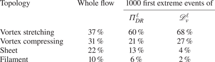
The global distribution of topologies can now be compared with the distribution of topologies among the 1000 strongest events of  $|\Pi ^\ell _{DR}|$ in order to check whether a particular topology is favoured by the extreme events of $|\varPi _{DR}^\ell |$, which may come together with inertial dissipation. The percentage of each topology among the 1000 strongest events of $|\Pi ^\ell _{DR}|$ is given in the third columns of tables 3 and 4 for $\ell _c/\eta =8$ and $\ell _c/\eta =150$ respectively. At $\ell _c/\eta =150$, extreme events of $|\Pi ^\ell _{DR}|$ cannot be associated with possible non-viscous dissipation because $\ell _c$ is too large, but we give their values to compare the behaviour of $\Pi ^\ell _{DR}$ in the dissipative and inertial ranges. The vortex stretching topology is clearly favoured among extreme events of $|\varPi _{DR}^\ell |$. This is especially pronounced in the dissipative range. We also give the distribution of topologies among the 1000 strongest events of $\mathscr {D}^\ell _{\nu }$. Extreme events of $\mathscr {D}^\ell _{\nu }$ seem to favour the vortex stretching topology too, even more than extreme events of $|\varPi _{DR}^\ell |$. The real-eigenvalued topologies are much less probable than among the 1000 strongest events of $|\varPi _{DR}^\ell |$.
Extreme events of  $|\Pi ^\ell _{DR}|$ and $\mathscr {D}^\ell _{\nu }$ favour the vortex stretching at the expense of the other topologies. One can therefore wonder whether these terms depend on the topology, i.e. on $Q$ and $R$. This can be investigated by studying the conditional averages of $\Pi ^\ell _{DR}$ and $\mathscr {D}^\ell _{\nu }$ conditioned on $Q$ and $R$. They are plotted in figure 5 for $\ell _c/\eta =8$ and $\ell _c/\eta =150$. Although they are scattered on the sides (large $|Q|$ and $|R|$), which is expected as such events are rare and do not allow for convergence of the conditional average, clear trends can be observed for smaller values of $|Q|$ and $|R|$. The largest values of $|\Pi ^\ell _{DR}|$ seem to be obtained in the sheet topology area both in the dissipative ( $\ell _c/\eta =8$) and inertial ranges ( $\ell _c/\eta =150$). This is quite at variance with the distribution of extremes conditioned on the 1000 strongest events of $|\varPi _{DR}^\ell |$. However, a zone of large $|\Pi ^\ell _{DR}|$ can be observed in the vortex stretching zone, at large negative values of $R$, for $Q$ around or slightly less than 0 (with smaller values than in the sheet zone, however). This zone corresponds to small values of $Q$, meaning that the enstrophy is dominated by the strain. The extreme events of $|\Pi ^\ell _{DR}|$ corresponding to vortex stretching probably come from this area. The conditional average of $\Pi ^\ell _{DR}$ is not the same in the dissipative and in the inertial range. In particular, the zone of negative $\Pi ^\ell _{DR}$ is in the vortex compressing area in the dissipative range, whereas it is in the vortex stretching area in the inertial range. This shows that the value of $\Pi ^\ell _{DR}$ does not depend only on the topology (i.e. $Q$ and $R$). The conditional average of $\mathscr {D}^\ell _{\nu }$ is more consistent with the distribution of the four topologies among the 1000 strongest events of $\mathscr {D}^\ell _{\nu }$: the conditional average of $\mathscr {D}^\ell _{\nu }$ takes large values in the vortex stretching zone, both for very large values of $Q$ and in the area where large values of the conditional average of $\Pi ^\ell _{DR}$ were observed, and in the vortex compressing zone. The isolines of the conditional average of $\mathscr {D}^\ell _{\nu }$ resemble the $QR$ joint p.d.f. isolines.
Conditional average of  $\Pi ^\ell _{DR}$ and $\mathscr {D}^\ell _{\nu }$ conditioned on the VGT second and third invariants $Q$ and $R$. The white lines correspond to the $QR$ joint p.d.f. isovalues. The red lines correspond to $\langle \varPi _{DR}^\ell \rangle _{Q,R}=0$. The black plain line corresponds to the Vieillefosse line $27R^2+4Q^3=0$. (a) Conditional average of $\Pi ^\ell _{DR}$ for $\ell _c/\eta =8$ (case T4). (b) Conditional average of $\Pi ^\ell _{DR}$ for $\ell _c/\eta =150$ (case T1). (c) Conditional average of $\mathscr {D}^\ell _{\nu }$ for $\ell _c/\eta =8$ (case T4). (b) Conditional average of $\mathscr {D}^\ell _{\nu }$ for $\ell _c/\eta =150$ (case T1).
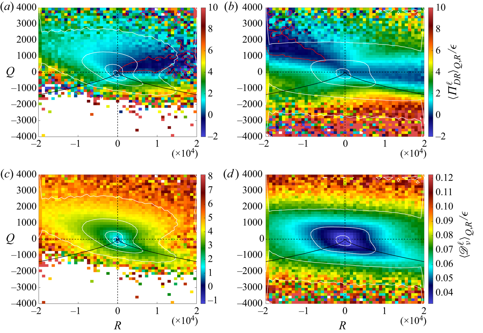
The analysis of the VGT invariants showed that the extreme events of  $|\Pi ^\ell _{DR}|$ mainly correspond to a zone of the vortex stretching area where the strain dominates the enstrophy. Such an analysis gives only information at the point where the extreme value is found, but ignores the structure velocity field around it. In the next section, we describe the structures of the velocity field observed around these extreme points.
5. Characterization by direct observation of the velocity fields
In order to characterize the velocity field on a larger area around the extreme events of  $|\varPi _{DR}^\ell |$, we observed:
(i) the velocity streamlines;
(ii) the
$\Pi ^\ell _{DR}$ and $\mathscr {D}^\ell _{\nu }$ fields; and(iii) and the isosurfaces of the vorticity;


for the ten strongest  $|\Pi ^\ell _{DR}|$ events and for each case.
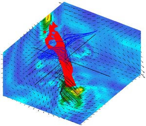
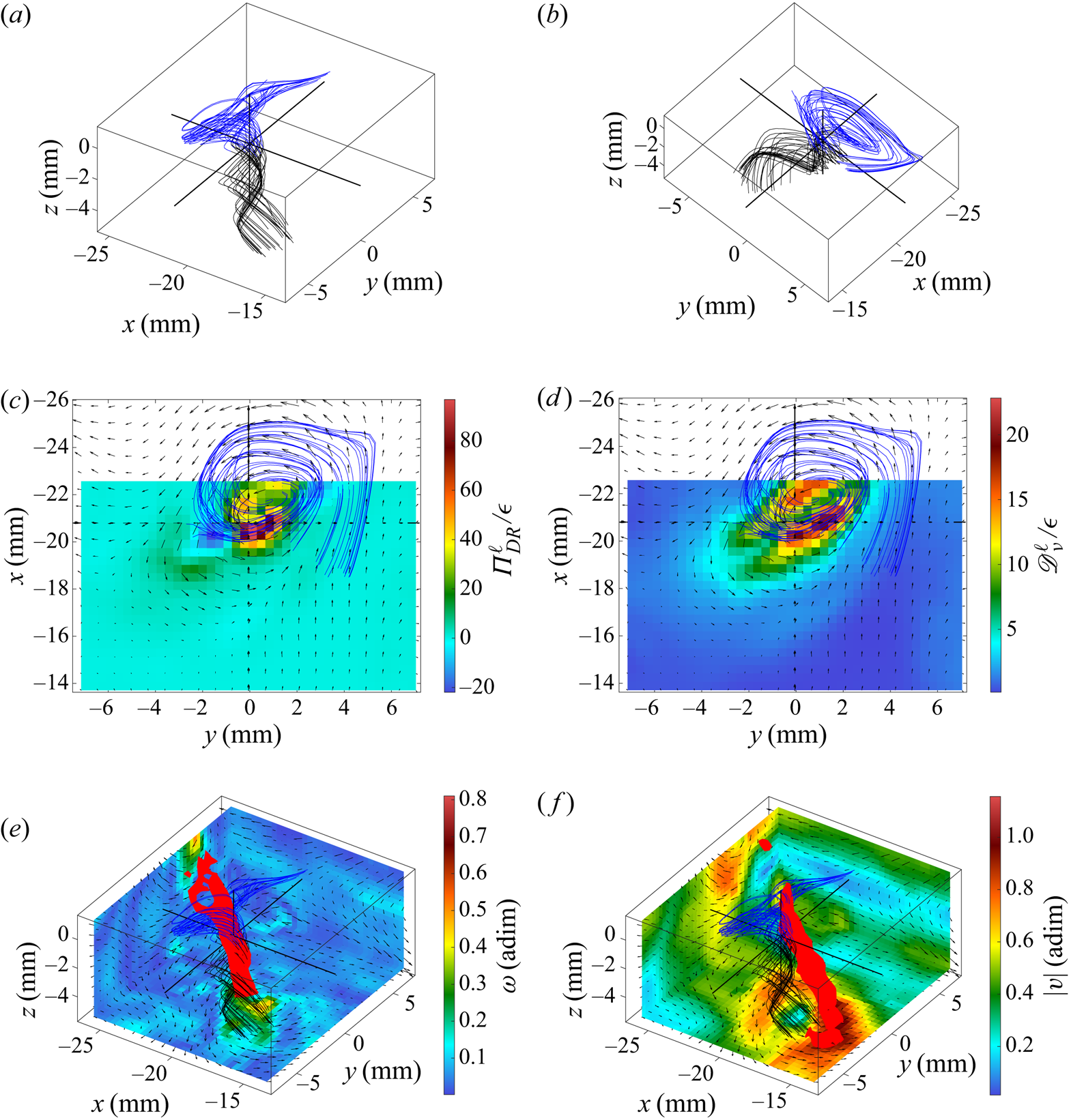
For case T4, i.e. when the dissipative scales are resolved by our measurement method, we observed three kinds of structures: the ‘screw vortex’, the ‘roll vortex’ and the ‘U-turn’. The screw vortex is characterized by streamlines that spiral in a single direction, whereas the roll vortex is characterized by streamlines that roll-up and then spiral in two opposite directions. An example of a screw vortex is shown in figure 6 and an example of a roll vortex is shown in figure 7. The U-turn is characterized by a sharp bend of the streamlines; an example is shown in figure 8. For all structures,  $\Pi ^\ell _{DR}$ takes large positive and negative values along the structure, but in the case of U-turns, the largest $|\Pi ^\ell _{DR}|$ corresponds to a negative $\Pi ^\ell _{DR}$ whereas for the vortices it corresponds either to a positive or negative $\varPi _{DR}^\ell$. All structures display large values of the velocity (three times the r.m.s. of the fluctuations). This is in accordance with the predicted divergence of the velocity norm in the case of a singularity occurring in a solution to the 3-D INSE (Constantin Reference Constantin2008), which would be the source of inertial dissipation. The observed structures also display large values of the vorticity (of the order of the maximum vorticity observed in all the velocity fields, i.e. 20 to 30 times the standard deviation of the vorticity) and of $\mathscr {D}^\ell _{\nu }$ (of the order of the maximum $\mathscr {D}^\ell _{\nu }$ observed in all the velocity fields, i.e. 30 times the standard deviation of $\mathscr {D}^\ell _{\nu }$). Actually, some of the ten strongest events of $|\varPi _{DR}^\ell |$ are also among the 10 strongest events of vorticity or of $\mathscr {D}^\ell _{\nu }$. In the case of the screw and roll vortices, the isosurfaces of the vorticity are tubes; in the case of U-turns, they are either tubes or pancakes. The parameter $\mathscr {D}^\ell _{\nu }$ takes large values around but outside of the zones of large vorticity; zones of large $\mathscr {D}^\ell _{\nu }$ are also shifted compared to zones of large $|\varPi _{DR}^\ell |$, they seem to better follow the symmetry of the structures compared to zones of large $|\varPi _{DR}^\ell |$.
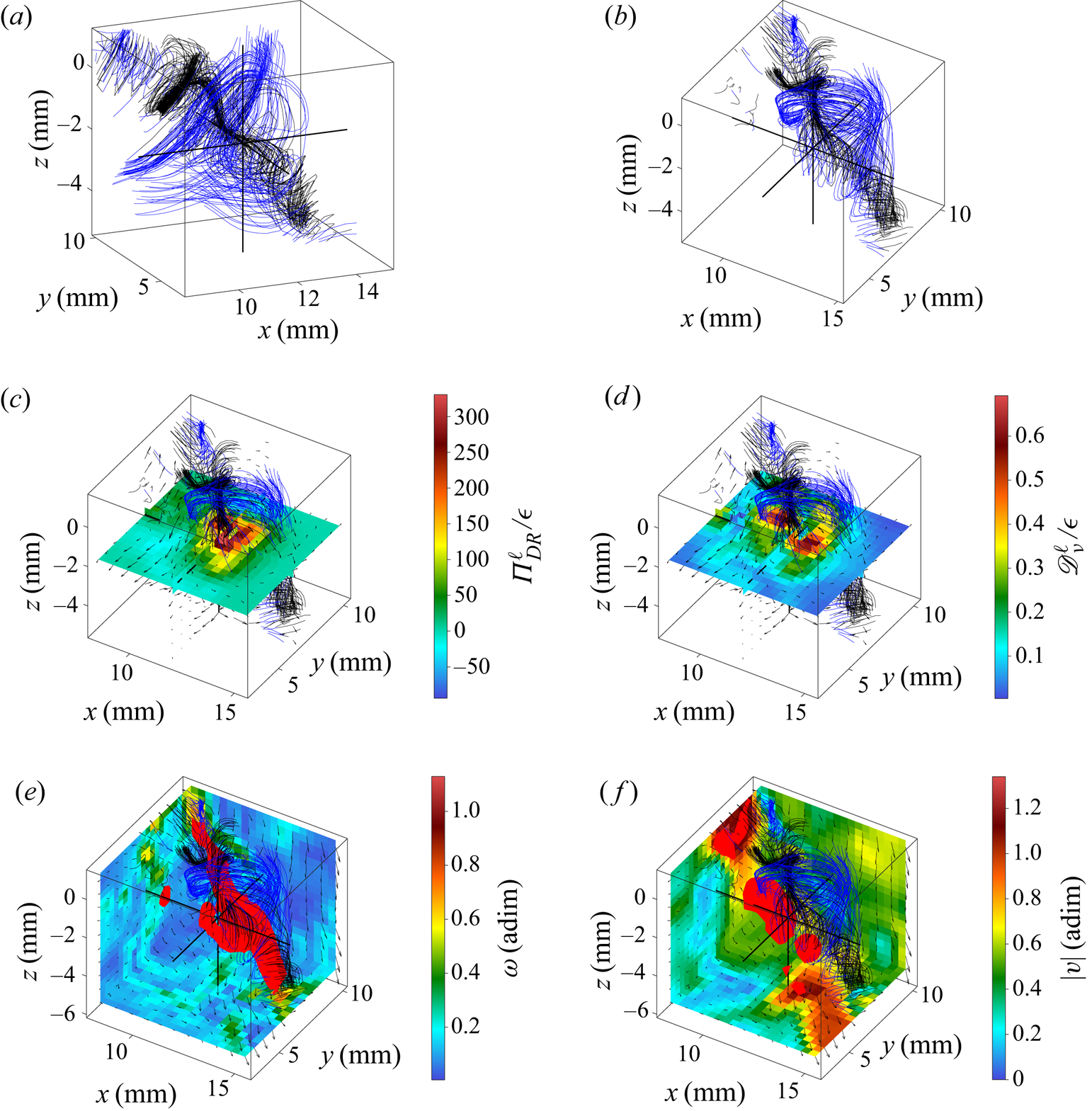
Velocity field around the first extreme event of  ${\varPi }_{DR}^\ell$ of case T4. (a) Velocity streamlines. (b) Velocity streamlines from another point of view. (c) In-plane velocity field (arrows) and ${\varPi }_{DR}^\ell$ field (colour) in the (xy) plane containing the extreme event. (d) In-plane velocity field (arrows) and ${\mathscr {D}}_{\nu }^\ell$ field (colour) in the (xy) plane containing the extreme event. (e) In-plane velocity field (arrows) in three (xy), (xz) and (yz) planes bounding the observed area, vorticity norm (colour on these planes), velocity streamlines and isosurface of the vorticity norm (isolevel: 0.41). (f) In-plane velocity field (arrows) in three (xy), (xz) and (yz) planes bounding the observed area, velocity norm (colour on these planes), velocity streamlines and isosurface of the velocity norm (isolevel: 0.92). Blue streamlines are arriving around the extreme event of ${\varPi }_{DR}^\ell$ whereas black ones are leaving the extreme zone.
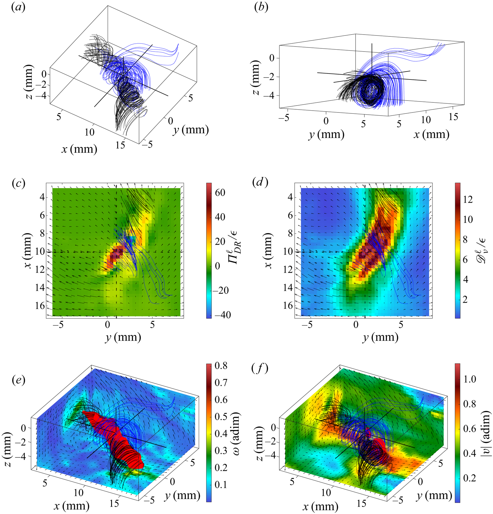
Velocity field around the fifth extreme event of  ${\varPi }_{DR}^\ell$ of case T4. (a) Velocity streamlines. (b) Velocity streamlines from another point of view. (c) In-plane velocity field (arrows) and ${\varPi }_{DR}^\ell$ field (colour) in the (xy) plane containing the extreme event. (d) In-plane velocity field (arrows) and ${\mathscr {D}}_{\nu }^\ell$ field (colour) in the (xy) plane containing the extreme event. (e) In-plane velocity field (arrows) in three (xy), (xz) and (yz) planes bounding the observed area, vorticity norm (colour on these planes), velocity streamlines and isosurface of the vorticity norm (isolevel: 0.33). (f) In-plane velocity field (arrows) in three (xy), (xz) and (yz) planes bounding the observed area, velocity norm (colour on these planes), velocity streamlines and isosurface of the velocity norm (isolevel: 0.77). Blue streamlines are arriving at zones of large vorticity whereas black ones are leaving such zones.
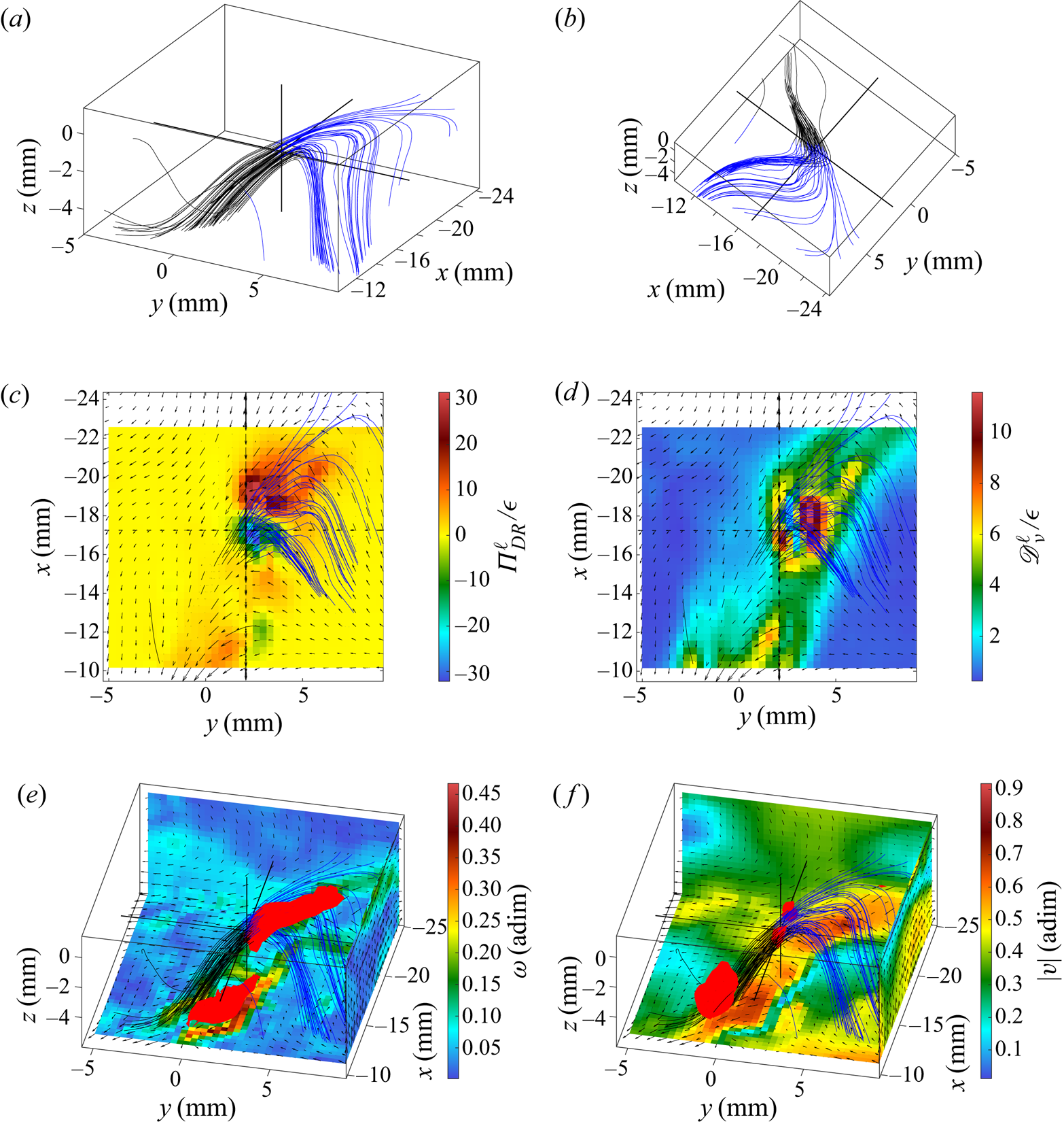
Velocity field around the fifth negative extreme event of  ${\varPi }_{DR}^\ell$ of case T4. (a) Velocity streamlines. (b) Velocity streamlines from another point of view. (c) In-plane velocity field (arrows) and ${\varPi }_{DR}^\ell$ field (colour) in the (xy) plane containing the extreme event. (d) In-plane velocity field (arrows) and ${\mathscr {D}}_{\nu }^\ell$ field (colour) in the (xy) plane containing the extreme event. (e) In-plane velocity field (arrows) in three (xy), (xz) and (yz) planes bounding the observed area, vorticity norm (colour on these planes), velocity streamlines and isosurface of the vorticity norm (isolevel: 0.33). (f) In-plane velocity field (arrows) in three (xy), (xz) and (yz) planes bounding the observed area, velocity norm (colour on these planes), velocity streamlines and isosurface of the velocity norm (isolevel: 0.77). Blue streamlines are arriving around the extreme event of ${\varPi }_{DR}^\ell$ whereas black ones are leaving the extreme zone.
For cases T1 to T3, i.e. when only the inertial scales are resolved by our measurement technique, similar structures were found except that they were more distorted or more complex: globally, it is possible to recognize one of the three structures mentioned above but fluctuations at smaller scales could be observed. This is consistent with the fact that the resolution is larger than the dissipative scales for these cases, and therefore that there exist fluctuations over scales smaller than the resolution. An example of a roll vortex is shown in figure 9: it is possible to distinguish the streamlines that roll-up and then spiral in two opposite directions, but the structure is twisted and less smooth than in the roll vortex in figure 7.
Velocity field around the first extreme event of  ${\varPi }_{DR}^\ell$ of case T1. (a) Velocity streamlines. (b) Velocity streamlines from another point of view. (c) In-plane velocity field (arrows) and ${\varPi }_{DR}^\ell$ field (colour) in the (xy) plane containing the extreme event. (d) In-plane velocity field (arrows) and ${\mathscr {D}}_{\nu }^\ell$ field (colour) in the (xy) plane containing the extreme event. (e) In-plane velocity field (arrows) in three (xy), (xz) and (yz) planes bounding the observed area, vorticity norm (colour on these planes), velocity streamlines and isosurface of the vorticity norm (isolevel: 0.68). (f) In-plane velocity field (arrows) in three (xy), (xz) and (yz) planes bounding the observed area, velocity norm (colour on these planes), velocity streamlines and isosurface of the velocity norm (isolevel: 1.13). Blue streamlines are arriving around the zones of large ${\varPi }_{DR}^\ell$ whereas black ones are leaving such zones.
6. Discussion
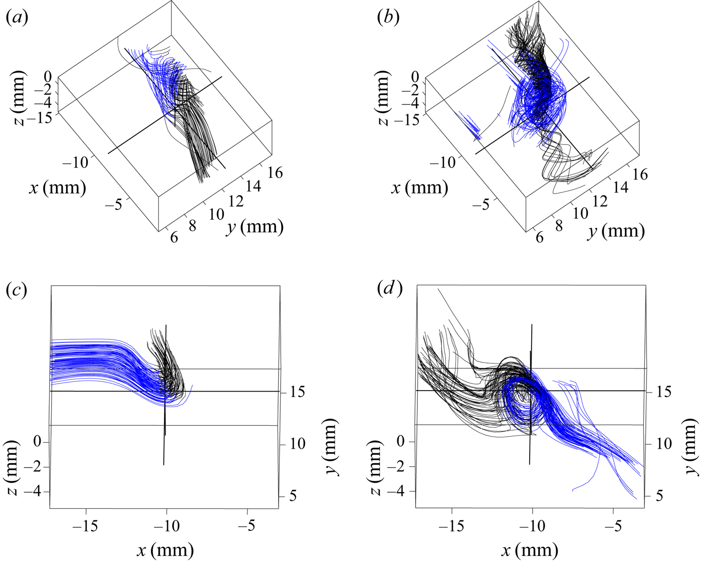
Three different kinds of structures seem to emerge from the analysis of the velocity fields around the extreme events of  $|\varPi _{DR}^\ell |$. However, in some cases, they may represent the same event, seen in different frames of reference or at different times. For instance, a roll vortex which is advected at a velocity oriented along its axis will look like a screw vortex in the laboratory frame of reference, as shown in figures 10(a) and 10(b). On the contrary, if it is advected at a velocity oriented perpendicularly to its axis, it will look like a U-turn in the laboratory frame, as shown in figures 10(c) and 10(d). Also, it is sometimes difficult to find the inertial frame in which a given structure would look like a roll vortex, and when the vorticity isosurfaces are pancake-like, in the case of some U-turns, it is impossible to find such an inertial frame: indeed, the vorticity is the same in any inertial frame, so it is not possible to find one where its isosurfaces would be tubes, as is expected from a roll vortex. However, it is possible that the three different structures correspond to a single one, seen at different times. For instance, in Vincent & Meneguzzi (Reference Vincent and Meneguzzi1994), the authors observe a roll-up of vorticity sheets, giving vorticity tubes. This suggests that a U-turn with pancake-like vorticity isosurfaces would appear first, and would evolve towards a U-turn with tube-like vorticity isosurfaces, followed by a vortex, whose vorticity isosurface is tube-like. Time-resolved measurements will allow for confirmation of this mechanism. Screw vortices may also be the remains of roll vortices after a possible split. Constructing formula for the observed topologies is not that easy because of limited spatial resolution in the $z$ direction; in a parallel unpublished numerical study of these events (Nguyen, Laval & Dubrulle Reference Nguyen, Laval and Dubrulle2020), we have, however, noticed that these structures bear some similarities with the asymmetric Burgers stretched vortices, studied in Moffatt, Kida & Ohkitani (Reference Moffatt, Kida and Ohkitani1994).
Impact of the frame of reference on the velocity field aspect. (a) Velocity streamlines around the second extreme event of  ${\varPi }_{DR}^\ell$ of case T4 seen in the laboratory frame of reference. (b) Velocity streamlines around the same event but in the frame of reference having a constant velocity (equal to the spatial average of the velocity over the observed field) with respect to the laboratory frame. (c) Velocity streamlines around the second negative extreme event of ${\varPi }_{DR}^\ell$ of case T4 seen in the laboratory frame of reference. (d) Velocity streamlines around the same event but in the frame of reference having a constant velocity (equal to the velocity at the extreme point) with respect to the laboratory frame. Blue streamlines are arriving towards zones of high vorticity whereas black ones are leaving such zones. The three black lines intersect at the point where ${\varPi }_{DR}^\ell$ is maximum.
Our results compare well with results in Saw et al. (Reference Saw, Kuzzay, Faranda, Guittonneau, Daviaud, Wiertel-Gasquet, Padilla and Dubrulle2016), where the structure of 2-D velocity fields around events of a 2-D version of  $\Pi ^\ell _{DR}$ is studied. Four 2-D structures where observed: spirals, cusps, fronts and jets. We could identify these four 2-D structures in particular cross-sections of our three 3-D structures. For instance, let us consider the sixth extreme event of ${\varPi }_{DR}^\ell$ of case T4, which is a roll vortex: a cross-section perpendicular to the vortex axis reveals a spiral (figure 11c) whereas a cross-section containing the vortex axis gives a front (figure 11a). Indeed, a roll vortex occurs when two bodies of fluid meet each other; one of them then rolls up and spirals in two directions. In a plane containing the axis, the spiral cannot be seen, contrary to the splitting in two directions: this is a front. Let us now consider the eighth negative extreme event of ${\varPi }_{DR}^\ell$ of case T4, which is a U-turn with a strong shear: looking at it from the front gives a cusp (figure 11d) whereas looking at it from the top reveals a jet (figure 11b).
Examples of the 2-D structures reported in Saw et al. (Reference Saw, Kuzzay, Faranda, Guittonneau, Daviaud, Wiertel-Gasquet, Padilla and Dubrulle2016) and observed in our results. The arrows correspond to the in-plane velocity field and the colour to the dimensionless term  ${\varPi }_{DR}^\ell$. (a) Front: top view of the sixth extreme event of ${\varPi }_{DR}^\ell$ of case T4. (b) Jet: top view of the eighth negative extreme event of ${\varPi }_{DR}^\ell$ of case T4. (c) Spiral: front view of the sixth extreme event of ${\varPi }_{DR}^\ell$ of case T4. (d) Cusp: front view of the eighth negative extreme event of ${\varPi }_{DR}^\ell$ of case T4.
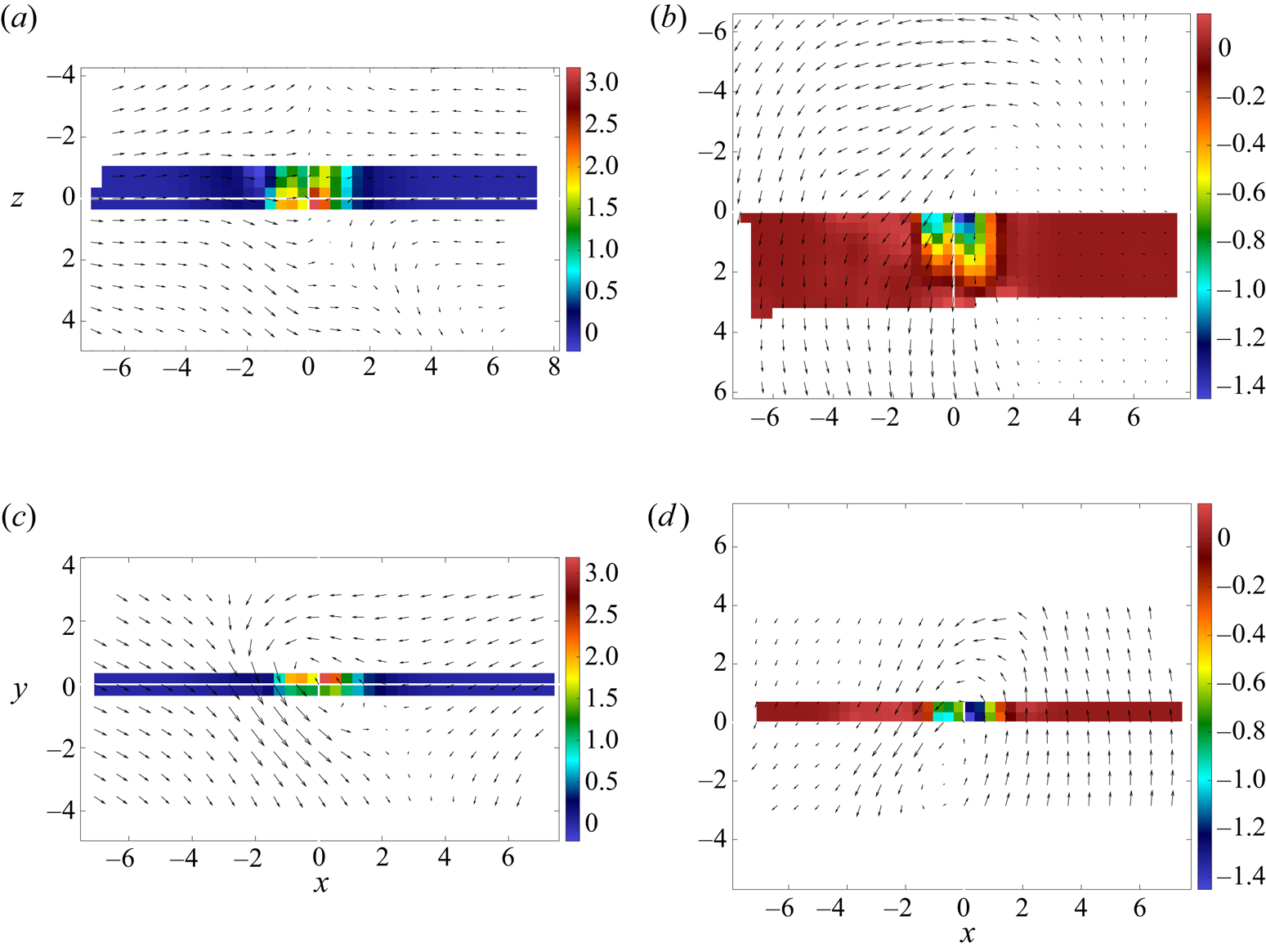
Our results also compare well with numerical works at similar Reynolds numbers: She, Jackson & Orszag (Reference She, Jackson and Orszag1990) ( $90^3$ grid, $R_\lambda =90$) and Vincent & Meneguzzi (Reference Vincent and Meneguzzi1991) ( $240^3$ grid, $R_\lambda =240$). Indeed, extreme events of $|\Pi ^\ell _{DR}|$ come with very large values of the vorticity, so that we can compare them with the large vorticity structures studied in those works. Note that it is not certain whether zones of large vorticity always come with large values of $|\Pi ^\ell _{DR}|$: it seems that large $|\Pi ^\ell _{DR}|$ leads to large vorticity norms, but the contrary remains to be proven. Both kinds of events may correspond to prints of singularities (see the Introduction and Beale, Kato & Majda Reference Beale, Kato and Majda1984), and the difference between them, if so, could shed some light on the problem. In accordance with those works, we observed that vorticity isosurfaces were either tubes or pancakes and that zones of large dissipation were surrounding the zones of large vorticity. This is at variance with more recent simulations with a larger Reynolds number (Yeung, Zhai & Sreenivasan Reference Yeung, Zhai and Sreenivasan2015) ( $8192^3$ grid, $R_\lambda \approx 1300$). In this work, stronger vorticity events are observed, with vorticity isosurfaces being blob-like and zones of large dissipation being colocated with zones of large vorticity. This colocation of the large vorticity and large dissipation zones is also observed in the stationary singular solutions of Li, Li & Yan (Reference Li, Li and Yan2018). The discrepancy between our experimental result and these numerical results may, however, be a spurious effect since it is known that they are very sensitive to the spatial and temporal resolution (Yeung, Sreenivasan & Pope Reference Yeung, Sreenivasan and Pope2018). In particular, the resolution of ${\rm \Delta} x=1.5 \eta$ used in the large Reynolds number simulation may not be sufficient, so that small scale structure may not be properly resolved. Indeed, intermittency of the dissipations calls for over-resolved simulations, for instance down to one tenth of the Kolmogorov scale (Dubrulle Reference Dubrulle2019). Note that this problem does not occur in our experiment because, even if the resolution measurement is around the Kolmogorov scale, smaller (unobserved) scales can nevertheless develop and impact the larger scales.
The fact that many of our events are associated with vortex compression might be a symptom of a link with vortex reconnection, as one might expect vortex compression immediately following such reconnection. We are currently preforming time-resolved measurements to confirm this point. Note that yet unpublished numerical work (Nguyen et al. Reference Nguyen, Laval and Dubrulle2020) indeed support such conjecture.
7. Conclusion
In this paper we studied the structure of the turbulent velocity fields around extreme events of  $\varPi _{DR}^\ell$ computed in the dissipative range. Such events may be precursors to non-viscous dissipation. We performed our analysis on 3-D velocity fields measured by TPIV at the centre of a von Kármán flow; at the smaller turbulent Reynolds number, our resolution is of the order of the Kolmogorov scale. The strongest $|\Pi ^\ell _{DR}|$ events we detected in the dissipative range reach 100 times the global average dissipation rate. We used two approaches to characterize the structure of the velocity field around these events: we studied the velocity gradient tensor invariants at the extremes and we observed the velocity fields and derived quantities. The conditional average of $\Pi ^\ell _{DR}$ conditioned on the VGT second and third invariants seems to be the largest in the sheet zone, but the most extreme events of $|\Pi ^\ell _{DR}|$ mostly correspond to the vortex stretching topology. The direct observation of the velocity fields allowed for identification of three different structures: the screw and roll vortices, and the U-turn. They may correspond to a single structure seen at different times or in different frames of reference. The extreme events of $|\Pi ^\ell _{DR}|$ come along with large velocity and vorticity norms, and the structure of the vorticity field around these events agrees with previous observations of numerical works at similar Reynolds numbers. It is at variance with more recent observations at larger Reynolds numbers, however. The agreement of our results with numerical results is encouraging and validates our experimental approach; time-resolved measurements are in progress to investigate the link between the three observed structures. Also, the relation between $\varPi _{DR}^\ell$ and the vorticity should be clarified, in order to check whether the detection criteria based on these two scalars are equivalent or whether the occurrence of both a large $|\Pi ^\ell _{DR}|$ and a large vorticity leads to special structures. Important headway regarding the problem of singularities would be made by checking whether the observed structures persist at even smaller scales or not. This will be achieved in a future work by improving the experimental resolution, together with investigations at larger Reynolds numbers as the occurrence of singularities may be conditioned on this parameter.
Acknowledgements
We thank anonymous referees for helpful comments, and M. Rossi for discussions about the structure of the velocity field around the extreme events. This work has been funded by the ANR, project EXPLOIT, grant agreement no. ANR-16-CE06-0006-01, and project ECOUTURB grant agreement no. ANR-16-CE30-0016.
Declaration of interests
The authors report no conflict of interest.


