

1. Introduction
One important feature of the development of the Brazilian agricultural frontier over the last decades is the conversion of pastures into cropland. Existing research indicates that this land use change is associated with substantial intensification of agricultural practices and improvements in socioeconomic indicators (e.g. VanWey et al., Reference VanWey, Spera, de Sa, Mahr and Mustard2013; Assunção and Bragança, Reference Assunção and Bragança2015). Nevertheless, there are concerns that pasture-to-cropland conversion might affect deforestation (e.g. Lapola et al., Reference Lapola, Schaldach, Alcamo, Bondeau, Koch, Koelking and Priess2010; Richards et al., Reference Richards, Walker and Arima2014). Therefore, understanding the environmental consequences of this change in land use is important to guiding public policies that combine economic development and forest conservation.
The Tapajós Basin seems to be the ideal context to examine these environmental consequences for at least two reasons. First, tropical forests cover 80 per cent of the region's area, underscoring the importance of understanding the determinants of deforestation in this region to mitigate global climate change (Stern, Reference Stern2007; Kindermann et al., Reference Kindermann, Obersteiner, Sohngen, Sathaye, Andrasko, Rametsteiner, Schlamadinger, Wunder and Beach2008; IPCC, 2014). Second, the region's agricultural production is becoming more important for Brazilian agricultural production, highlighting the potential conflict between changes in land use and forest conservation in this area (Rada, Reference Rada2013).
This paper provides evidence that pasture-to-cropland conversion generated positive environmental externalities at the local level in the Tapajós Basin during the period 2002–2012. The analysis uses variation in relative crop-to-beef prices as an exogenous source of variation in the relative return of soy cultivation and cattle ranching to estimate the local effects of land conversion on deforestation. The research design combines time series variation in prices with cross-sectional variation in initial production to build local price indexes for soy and beef. This procedure is based on the intuition that a change in the price of a product is more important in municipalities that are more specialized in this product's production.Footnote 1
The local soy and beef price indexes are used to construct a crop-to-beef relative price index. The baseline estimates regress deforestation on the relative price index conditional on a set of covariates, fixed effects, and state-specific trends. The covariates include the price indexes for each product to control for the effect of the price levels on overall agricultural expansion. This ensures that relative prices are capturing changes in the relative return across different land uses rather than the impact of changes in absolute price levels.
The results indicate that an increase in relative crop-to-beef prices generates an expansion in soy cultivation and a reduction in deforestation. The preferred specification suggests that an increase in one hectare in soy cultivation is connected to a decrease in 0.39 hectares in deforestation at the local level. The magnitude of this impact is substantial. It implies that the increase in 13,500 square kilometers in soy cultivation saved 5,300 square kilometers of tropical forests in the Tapajós Basin alone from the period 2002 to 2012. These localized effects of changes in land use represent almost 15 per cent of the observed deforestation in the period. The effect is concentrated in municipalities in the agricultural frontier in which intensive agriculture expanded quickly over the past decade without a sizeable reduction in forest coverage.Footnote 2
These estimates are robust to several alternative specifications. The magnitude of the coefficients changes little with the inclusion of additional covariates and the use of alternative price indexes. Statistical inference is also robust to different assumptions on the variance of the estimators. Moreover, outliers do not seem to drive the empirical results.
These findings are interpreted using a simple economic model describing land use choices in the region. In the model, farmers can either leave their land as forest or use it for two agricultural activities (crop cultivation and cattle ranching). The model assumes that crop cultivation is more intensive in capital (e.g., tractors, fertilizers) and labor (e.g., agronomists, agricultural technicians, tractor operators) than cattle ranching. This theoretical model predicts that a change in land use can affect deforestation through its effect on input prices. Input prices will increase if land allocation shifts towards the more input-intensive product and decrease if land allocation shifts towards the less input-intensive product. These changes in input prices will affect deforestation by affecting farmers' choice to clear forests. In particular, an increase in input prices will induce low productivity cattle ranchers to leave agriculture while a decrease in input prices will induce low productivity cattle ranchers to enter the sector. Deforestation will fall in the former scenario and grow in the latter.
The displacement effect discussed above is important to explain the environmental benefits associated with the expansion of intensive agriculture at the local level. The estimates point out that the positive local-level environmental externalities identified in this paper mitigate a substantial share of the negative spillover effects from cropland expansion discussed elsewhere in the literature (e.g. Lapola et al., Reference Lapola, Schaldach, Alcamo, Bondeau, Koch, Koelking and Priess2010; de Sa et al., Reference de Sa, Palmer and di Falco2013; Richards et al., Reference Richards, Walker and Arima2014). This result can have important implications for public policies as taxes and subsidies can be used to generate variation in relative returns across agricultural activities and induce changes in land use.
The evidence from this paper is connected to a growing literature that investigates the relationship between agriculture and deforestation. Assunção et al. (Reference Assunção, Lipscomb, Mobarak and Szerman2014) provides evidence that electrification also reduced deforestation in Brazil during the period 1960 to 2000. Assunção and Bragança (Reference Assunção and Bragança2015) documents that technological innovations reduced deforestation in Central Brazil during the period 1960 to 1985. These studies also suggest that agricultural intensification is the main mechanism connecting these episodes with mitigation of forest clearing. In the context of theae studies, changes in production possibilities affect farmers' choices and deforestation, whereas in this paper's context, changes in relative prices affects these variables.
The evidence from this paper is also related to the literature that discusses the impact of prices on deforestation in the Brazilian Amazon (Angelsen and Kaimowitz, Reference Angelsen and Kaimowitz1999; Pfaff, Reference Pfaff1999; Assunção et al., Reference Assunção, Gandour and Rocha2015). This literature discusses the role of absolute prices for deforestation in the region. This paper contributes to this literature by providing evidence that relative prices matter for deforestation. This paper is also related to Roberts and Schlenker (Reference Roberts and Schlenker2013), as it highlights that the prices of all agricultural products affect the land allocation for a given product.
The remainder of the paper is organized as follows. Section 2 describes the evolution of occupation and land use in the Tapajós Basin over the past decades. Section 3 presents an economic model to guide the empirical analysis. Section 4 describes the data sources and the empirical design used in the empirical estimates. Section 5 reports and discusses the main results. Section 6 reports the results from several robustness checks. Section 7 presents some concluding remarks on the results and their implications.
2. Background
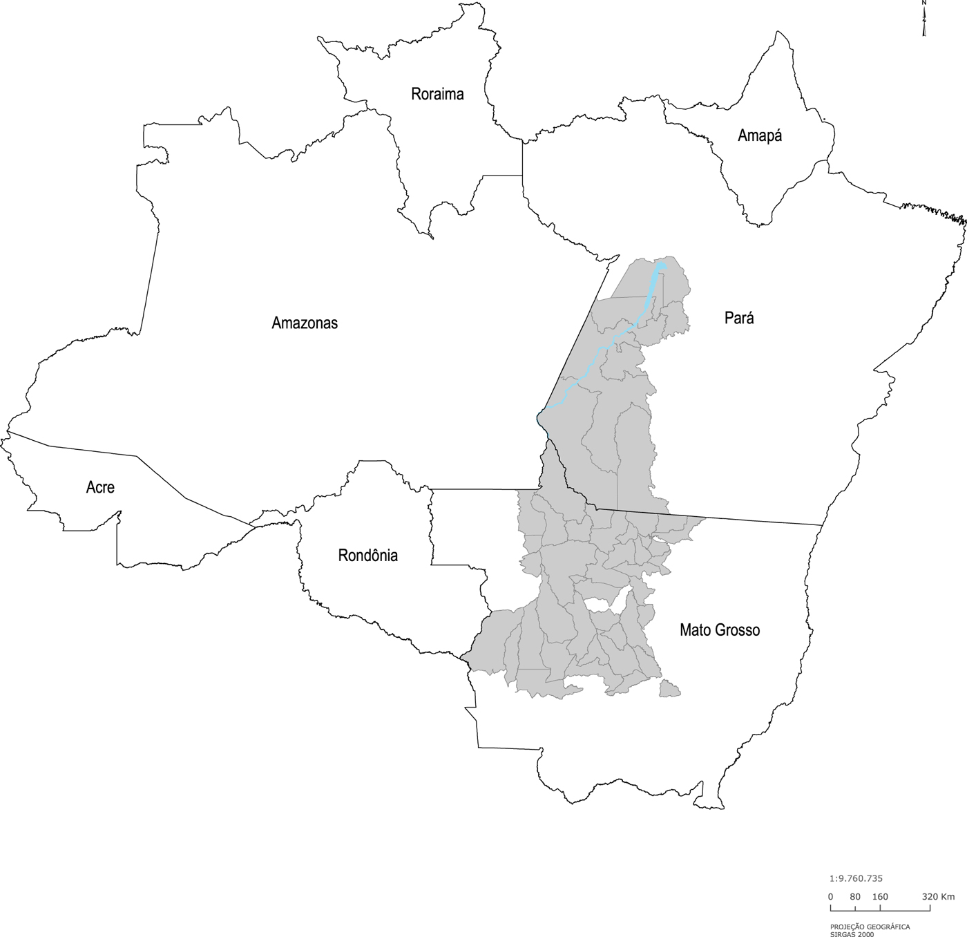
The Tapajós River is an important tributary of the Amazonas River. It is located in the southern Amazon, starting in the municipality of Juruena in the state of Mato Grosso and ending in the municipality of Santarém in the state of Pará. Its total length is 810 kilometers, and it is formed by the union of Juruena and Teles Pires rivers. According to the Brazilian Statistical Office (IBGE), the river forms a hydrographic basin covering 49 municipalities with an area exceeding 500,000 square kilometers.
The location of the river and its basin is presented in figure 1. The Tapajós Basin covers most of the northern areas of the state of Mato Grosso (57 per cent of its total area) as well as the southeastern areas of the state of Pará (43 per cent of its total area). The basin includes 40 municipalities in the former state and 9 municipalities in the latter.
The Tapajós Basin.
This region has increased in economic importance recently and has progressively become an important area for crop and beef production. The value of crop production in the Tapajós Basin increased from R$ 6.2 billion to R$ 13.7 billion from 2002 to 2012, whereas the number of cattle expanded from 7.2 to 10.9 million head during the same period.
Agricultural expansion has raised concerns regarding environmental degradation in the region. Approximately 80 per cent of the region's area was historically covered by forests. Of this, about 20 per cent was cleared until 2002 and an additional 27 per cent was cleared from 2002 to 2012. To give an idea of the concerns regarding deforestation in the region, the Tapaj ós Basin includes seven of the 41 municipalities in which the Brazilian Environmental authorities concentrate anti-deforestation efforts due to their high incidence of forest clearing.
These environmental concerns have increased due to the existence of large infrastructure projects across the region. The Brazilian government is sponsoring the construction of dams as well as the improvement of waterways and roads. These projects have faced substantial opposition from environmental organizations, which argue that further occupation and agricultural expansion in the region might generate further degradation. In particular, there is concern that transportation projects will reduce freight costs and, as a consequence, stimulate agricultural activities in the Tapajós Basin.
Changes in land use that lead to agricultural intensification offer an alternative to combining agricultural development with forest protection in the region. Therefore, it is important to understand whether changes in land use affect deforestation, in order to guide policies aimed at limiting environmental degradation in the region. The region's recent experience seems to be relevant to this evaluation given the extent of pasture-to-cropland conversion observed in the region over the last decades.
3. Economic model
Suppose there is a continuum of land owners of mass 1. Each land owner is indexed by i and holds a plot of size 1. A plot can be used either for cattle ranching (beef production) or crop cultivation (soy production). It can also be left idle in which case it remains as forest area. Land owners are heterogeneous and are characterized by a productivity parameter A i. This parameter is a function of the land owner's competence and/or the geographic characteristics of the plot. We assume that A i is distributed according to G(.) in the support [0, ∞].
The return from cattle ranching is A i, while the return from crop cultivation is Δ A i. The parameter Δ captures differences in return across the two activities. Assume that Δ > 1. Let the price of beef be P b and the price of soy be P s. Therefore, revenues under the different land uses are either P bA i or ΔP sA i.
Costs to use the plot are different in cattle ranching and in crop cultivation. We assume it costs l b units of labor and k b units of capital to use a plot as pasture and l s > l b units of labor and k s > k b units of capital to use it as cropland. Empirical evidence supports these assumptions and indicates that crop cultivation is more intensive in inputs than cattle ranching in the Brazilian agricultural frontier (Assunção and Bragança, Reference Assunção and Bragança2015).
Combining revenues and costs, we obtain the following profit functions under cattle ranching and crop cultivation:
 $$\eqalign{\pi _{b}(A_{i})&=P_{b}A_{i}-wl_{b}-rk_{b},}$$
 $$\eqalign{\pi _{s}(A_{i})&=\Delta P_{s}A_{i}-wl_{s}-rk_{s}.}$$
Farmers choose their plot's land use by comparing profits across different activities. Land will remain idle whenever π b(A i) < 0 and π s(A i) < 0. A plot will be used as pasture when π b(A i) > 0 and π b(A i) > π s(A i). It will be used as cropland when π s(A i) > 0 and π s(A i) ≥ π b(A i).
These inequalities can be combined to determine the sorting pattern of different farmers under different prices and parameter values. Assume that 1 < Δ(P s/P b) < (wl s − rk s)/(wl b − rk b). This assumption states that revenues in crop cultivation are higher than in cattle ranching. But this difference in revenues is not sufficient to compensate for differences in costs across all farmers. The following theorem characterizes land use under these conditions.
Theorem 1. Farmer's optimal land use choices can be summarized using the following conditions:
(i) Farmers will leave land idle when A i < A;
(ii) Farmers will use land as pasture $\underline{A} \leq A_{i} < \overline{A}$;
(iii) Farmers will use land as cropland
$A_{i} \geq \overline{A}$,


in which A = (w l b − r k b)/P b and  $\overline{A} = \lpar w \lpar l_{s}-l_{b}\rpar - r \lpar k_{s}-k_{b}\rpar \rpar /\lpar \Delta P_{s} - P_{b}\rpar $. 1
Proof See the online appendix A.
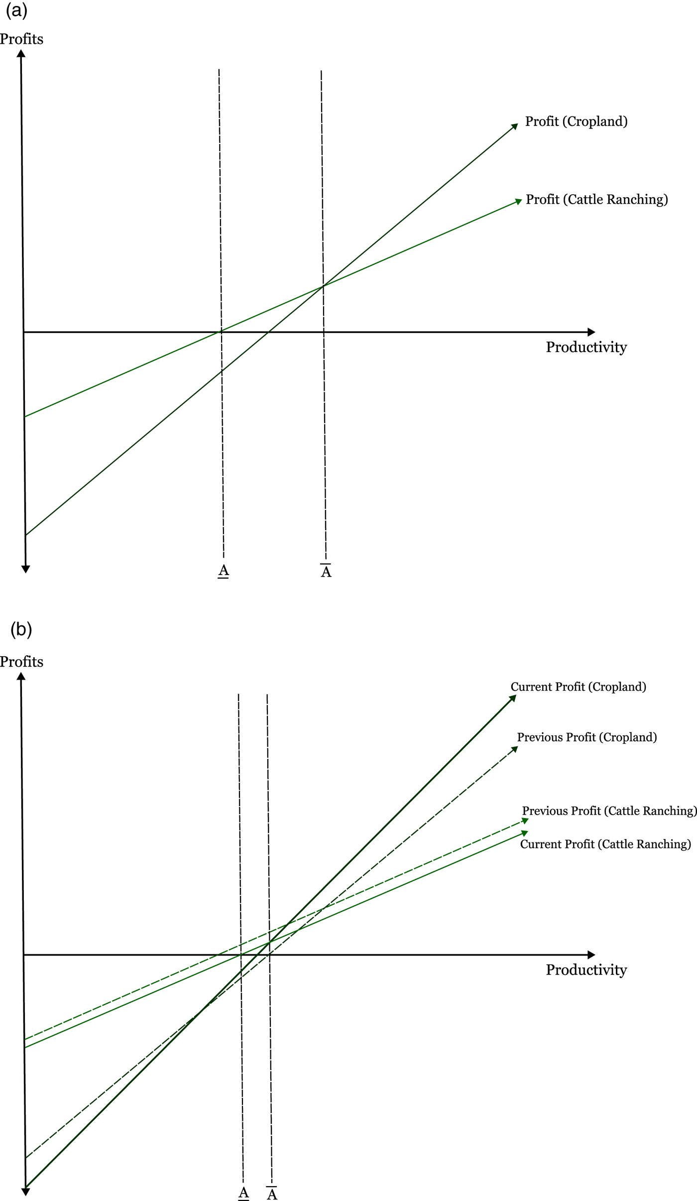
Figure 2a provides a graphical illustration of the results from theorem 1. Cattle ranching profits are depicted by the green line, and crop cultivation profits are depicted by the dark green line. Profits increase as farmers become more productive. The intersection between cattle ranching profits and the horizontal axis determines the threshold A above which cattle ranching is profitable. Notice that at this point, profits in cattle ranching are higher than profits in crop cultivation.Footnote 3 This situation persists until the intersection between the cattle ranching and crop cultivation profits. This intersection determines the threshold  $ \overline{A}$ above which crop cultivation is more profitable than cattle ranching. The thresholds A and $\overline{A}$ characterize the farmers' choices. Individuals with low productivity (below A) will leave their land idle, individuals with intermediate productivity (above A and below $\overline{A}$) will use their plots as pastures, and individuals with high productivity (above $\overline{A}$) will use their plots as cropland.
Equilibrium. (a) Optimal Choices (b) Effects of an Increase in Relative Prices.
Theorem 1 enables us to define the equilibrium share of forests (A f = G(A)), pastures ( $A_{b}=G\lpar \overline{A}\rpar -G\lpar \underline{A}\rpar $) and cropland ( $A_{s}=1-G\lpar \overline{A}\rpar $). These equilibrium shares determine the demand for labor and capital in the agricultural sector:
 $$D_l(w) = l_sA_s + l_bA_b\;{\rm and}\;D_k(r) = k_sA_s + k_bA_b.$$
 Factor prices are determined by combining the demand curves above with the local supplies of labor and capital. The paper assumes that there is spatial segmentation across municipalities. Segmentation reflects the existence of moving costs or information asymmetries in the financial sector. Supply curves will be positively related to factor prices under this assumption. Let labor supply be S l(w) (with  $S_{l}^{^{\prime }}\lpar w\rpar >0$) and the capital supply be S k(r) (with $S_{k}^{^{\prime }}\lpar r\rpar >0$). Market clearing implies:
 $$D_l(w) = S_l(w)\;{\rm and}\;D_k(r) = S_k(r).$$
The competitive equilibrium in the model is the set (A f, A b, A s, w, r) such that land use is optimal and equation (3) holds. The following theorem establishes the effect of a change in crop-to-beef prices in the model's equilibrium.
Theorem 2. An increase in the relative crop-to-beef price induces pasture-to-cropland conversion (As increases and Ab decreases) and reduces deforestation (Af increase).
Proof See online appendix A.
Figure 2b presents the intuition of theorem 2. Dashed lines represent profit curves in the initial situation whereas solid lines represent profit curves after the increase in relative prices. An increase in the relative price makes the profit curve for crop cultivation steeper. This induces farmers to convert pastures into cropland and increases the total demand for labor and capital and their respective equilibrium prices. These price increases shift the profit curves down for both cattle ranching and crop cultivation. The downward shift in cropland profits reduces the incentives that farmers have to convert pastures into cropland. However, in equilibrium, some farmers will still be induced to convert their pastures into cropland, and the threshold  $\overline{A}$ will fall. In addition, the downward shift in cattle ranching profits will induce some farmers to stop ranching and leave their land idle and the threshold A will increase. These changes in the sorting behavior across agricultural activities lead to increases in cropland (A s) and forests (A f) and decreases in pastures (A b).
4. Data and empirical design
4.1 Data sources
The main outcome used throughout the empirical analysis is the deforestation rate. Deforestation data comes from satellite images processed in the realm of the Project for Monitoring Deforestation in the Brazilian Amazon (PRODES–Projeto de Monitoramento do Desmatamento da Amazônia Legal). The PRODES team examines the raw satellite images to spot deforested areas located throughout the Brazilian Amazon. Images are compared across periods to determine which polygons have been cleared in a given period. These polygons are combined to produce municipal level measures of deforestation covering all municipalities of the region. It is important to note that PRODES coverage is affected by the presence of clouds and non-observed areas.
The analysis uses deforestation data covering the period 2002 to 2012 across the 49 municipalities located in the Tapajós Basin. Deforestation in year t is the total forest area cleared from August 1 in year t − 1 to July 31 in year t. The total deforestation is divided by the municipal area to calculate the share of the municipal area cleared in a given period. This is the main dependent variable used in this paper. Other variables from the PRODES dataset are used as controls in some specifications. These variables are initial forest area, non-observed areas and cloud presence.
In order to examine the effect of relative prices on deforestation, local price indexes are constructed for the main agricultural products in the region (soy and beef). Each price index is constructed combining price information P ot of the product o in period t with the initial production S mo of this product in municipality m,
 $$\eqalign{ p_{mot}={P}_{ot}{S}_{mo}\,,}$$
in which p mot is the price index for each product (o = {b, s} in which b denotes beef and s denotes soy). These price indexes can be interpreted as ‘Laspeyres price indexes’ because of the use of initial information. In the baseline specification, S mo is defined as the ratio between the number of cattle and the municipal area for the case of beef and as the ratio between the soy area and the municipal area. Data from 2000–2001 is used to define these measures of initial production. These price indexes are combined to produce the relative crop-to-beef price index P mt which is the main independent variable in the empirical exercises. This variable is defined as:
 $$P_{mt} = \displaystyle{{p_{mst}} \over {p_{mbt}}}.$$
All price indexes are standardized (mean equal to zero and variance equal to one). The robustness exercises consider three different methods for constructing the relative prices. First, instead of data on soy acreage and beef production in the beginning of the period under analysis (2000–2001), data on soy acreage and beef production in the end of the period under analysis (2010–2012) is used to construct the S mb and S ms. Second, instead of data on soy acreage, data on soy and maize acreage is used to compute S ms. Third, instead of data on soy prices, data on the average soy and maize prices is used to calculate p mst.
Data on agricultural prices comes from the Secretaria de Agricultura do Paran á, which collects monthly prices of several agricultural products. Notice that such prices are exogenous to local growing conditions in the Tapajós Basin. Data on initial production comes from the Pesquisa Agr ícola Municipal and the Pesquisa Pecuária Municipal. The Pesquisa Agrícola Municipal provides yearly information on area, production, and production value for all crops and municipalities in Brazil. The Pesquisa Pecuária Municipal provides information on the cattle stock across all municipalities in Brazil. Both datasets are collected from the IBGE. These datasets are also used to calculate the change between periods in soy area and the number of cattle. These variables are important when examining whether changes in relative prices are mapped in changes in land use as suggested in the theoretical model.
Information from other sources are used as controls in some empirical specifications. Data on initial economic environment comes from the 1995/1996 Agricultural Census, the 2000 Population Census, and the NEMESIS/IPEA. Data on the number of bank branches in each municipality comes from administrative data of the Brazilian Central Bank. Data on the number of beneficiaries of the program Luz para Todos–a large-scale electrification program–comes from the Brazilian Ministry of Mining and Energy. Data on the number of land reform projects is constructed using administrative information on land reform projects provided by the Brazilian Ministry of Agriculture. Data on the share of the municipal area covered by protected areas is constructed using GIS information from the Brazilian Ministry of the Environment.
4.3 Descriptive statistics
Table 1 reports descriptive statistics for the main dependent variables that are used throughout the paper. Column 1 presents the sample average in 2002 while column 2 depicts the sample average in 2012. Column 3 reports the increase between these periods. Total deforestation grew from 16 per cent to 21.5 per cent of the average municipal area in the period 2002 to 2012. The increase in deforestation was accompanied by increases in total cropland from 6.5 per cent to 11.9 per cent of the average municipal area. This expansion in cropland was driven by expansion in soy and maize cultivation (respectively, from 4.5 per cent to 7.2 per cent and from 0.9 per cent to 3.0 per cent of the average municipal area). The Tapajós Basin also experienced an expansion in cattle ranching during this period as the number of cattle per square kilometer grew from 14 to 21 head. As the Pesquisa Agrícola Municipal does not contain information on pastures, it is not possible to know whether this increase in cattle ranching was a result of changes in the intensive or the extensive margin.
Descriptive statistics

Notes: Standard deviations are reported in brackets. Observations are computed using data from all 49 municipalities in the Tapajós Basin and are weighted by municipal area.
Data on prices indicates increases in soy and beef prices during this period. Growth in soy prices was smaller than in beef prices, with relative prices falling a little. This is the main relative prices measure studied in this paper. Notice that maize prices are excluded in calculating the relative price index despite the importance of maize in total cropland. This is done because most maize cultivated in the region is cultivated in a second growing season (safrinha) and its cultivation is more related to soy prices than maize prices.
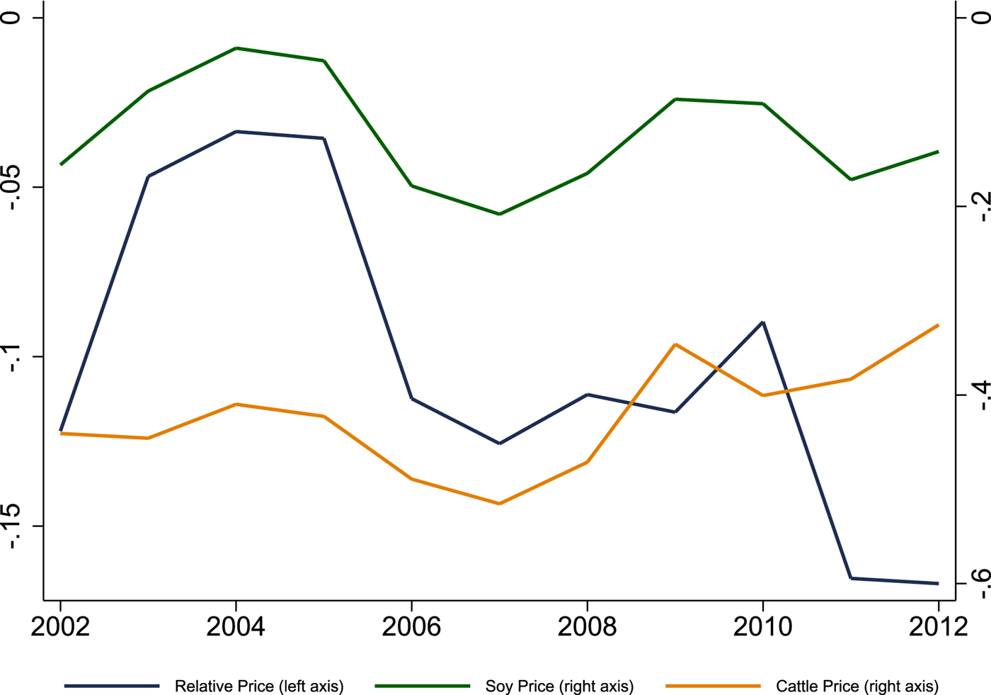
Figure 3 depicts the variation in prices throughout the whole period to present a more complete picture of price variation. Relative prices increase from 2002 to 2005 and decrease afterwards. From 2005 to 2007, the decline in relative prices is due to a larger drop in soy prices compared to beef prices. From 2008 to 2010, the variation in relative prices is connected to larger increases in beef prices compared to soy prices. In 2011 and 2012, the change in relative prices is caused by the decrease in soy prices and the small increase in beef prices.
Price variation.
The figures in online appendix B report the basic correlations between relative prices and land use. Online appendix figure A1 presents the correlation between relative prices and deforestation. Increases in relative prices are correlated with decreases in deforestation as suggested in the theoretical model. An increase in one standard deviation in relative prices is associated with a decrease in 18 per cent of a standard deviation in annual deforestation (0.14 square kilometers). Figure A2 (online appendix) reports that increases in relative prices are also correlated with increases in soy cultivation and decreases in the number of cattle. Therefore, the structure of the data seems to indicate that pasture-to-cropland conversion is associated with lower deforestation. However, it is important to view this evidence with caution since it can be a result of omitted variable bias.
4.3 Empirical design
To investigate the causal effect of land use on deforestation in the Tapaj ós Basin, the research design uses exogenous variation in prices. The baseline analysis regresses deforestation y on municipality m and period t on the crop-to-beef relative price index P in the previous period controlling for fixed effects:
 $$y_{mt}=\beta P_{mt-1}+\alpha _{i}+\theta _{t}+\varepsilon _{mt}.$$
The price definition uses initial exposures variables (cropland area and number of cattle) to construct the municipal relative price index. This can create spurious correlation between relative prices and deforestation to the extent that the initial exposure variables can influence changes in y mt over time. To mitigate this concern, state-specific trends (ρs* t ) and a set of covariates (Xmt) are added as additional controls in the empirical model:
 $$y_{mt} = \beta P_{mt - 1} + {\gamma }^{\prime}{\bf X}_{{\bf mt}} + \alpha _i + \theta _t + \rho _s*t + \varepsilon _{mt}.$$
The baseline specification includes price levels, initial deforestation interacted with time dummies, and areas non-observed or covered with clouds in the vector Xmt. These price levels control for the effect of absolute prices on deforestation, enabling an examination of the effect of changes in relative returns across land uses rather than changes in overall agricultural returns. The initial deforestation interacted with time dummies controls for arbitrarily different trends in deforestation associated with initial differences in forest area. Cloud coverage and non-observed areas control for non-classical measurement error in deforestation.
The identification assumption on equation (5) is that–in the absence of changes in relative prices–changes in deforestation would be similar across municipalities located in the same state and with comparable soy and beef price indexes and initial forest area. It is important to notice that relative prices decrease and increase multiple times during the period under analysis. This implies that identification of the effect of relative prices on deforestation using the research design described above is not coming from convergence or divergence in deforestation rates across municipalities with different initial economic environments. Moreover, it implies that the roll out of infrastructure projects and other government policies omitted from this equation is unlikely to drive the results since these investments and policies are not easily reversed.
Nevertheless, different checks are performed to examine the robustness of the identification assumption discussed above. The first set of robustness tests includes variables describing the initial economic environment (e.g., transportation costs, mechanization, land tenure, wages) interacted with time dummies in the vector Xmt to investigate whether convergence or divergence in deforestation rates influence the results. The second set of robustness tests includes measures of investments in infrastructure and the roll out of important government policies in the vector Xmt to examine whether these investments or policies influence the results.
The regressions typically weight observations using the square root of the municipal area as in Schlenker et al. (Reference Schlenker, Hanemann and Fisher2006) and Deschênes and Greenstone (Reference Deschênes and Greenstone2007). Standard errors are clustered at the municipal level to correct for the existence of serial correlation in our price index (Bertrand et al., Reference Bertrand, Duflo and Mullainathan2004). Evidence is provided that the results are robust to using the municipal area as weights and to not using weights at all. Evidence is also provided that the results are robust to using the Conley (Reference Conley1999) standard errors that allow for spatial dependence in the error term.
Additional regressions use specifications similar to equations (4) and (5), but using crop cultivation and number of cattle as the dependent variables. Estimation using these dependent variables requires the same identification assumptions discussed above.
5. Results
5.1 Relative prices and pasture-to-crop conversion
Table 2 reports evidence on the relationship between relative prices and agricultural activities in the Tapajós Basin. Columns 1 to 3 depict the impact of relative prices on soy cultivation while columns 4 to 6 depict this impact on the number of cattle. Soy cultivation refers to the change in the share of the municipal area cultivated with soy, whereas the number of cattle refers to the change in the number of cattle per square kilometer.
Relative prices and agriculture

Notes: Each column reports the results of regressing the dependent variable on the soy-to-beef relative price index conditional on soy and cattle price indexes and a set of additional covariates. The soy price index is obtained by combining initial soy cultivation with aggregate price variation while the beef price index is obtained by combining initial number of cattle with aggregate price variation. All estimates use data from the 49 municipalities in the Tapajós Basin during the period 2002 to 2012. Observations are weighted by the square root of the municipal area. Standard errors clustered at the municipality level are reported in parentheses. ***p < 0.01 **p < 0.05 *p < 0.1.
Column 1 provides evidence that growth in relative soy-to-beef prices leads to an expansion in soy cultivation. The coefficient is significant at the 10 per cent level (p-value = 0.09) and its magnitude is substantial. One standard deviation increase in relative prices increases soy cultivation by 0.95 per cent of the total municipal area, which is about 40 per cent of a standard deviation in the annual change in soy cultivation. Column 1 shows that absolute soy prices also lead to an expansion in soy cultivation but that absolute cattle prices do not affect this variable.
Column 2 adds the initial forest area (as a percentage of the municipal area) interacted with time dummies as an additional covariate to examine whether the effect from column 1 is connected to initial differences in land use. This is a concern, to the extent that initial differences in land use can affect both the local price indexes and the changes in crop cultivation. The results indicate that the relationship between relative prices and soy cultivation is robust to this control. The coefficient on relative prices increases from 0.95 to 1.09 and remains significant at the 10 per cent level (p-value = 0.08). It is also interesting to note that the coefficients on absolute prices change much more than the coefficient on relative price. This suggests that differential trends is a much more important concern in interpreting these coefficients.
Column 3 further adds state-specific trends to investigate whether differences between the evolution of policies and economic environment in the states of Mato Grosso and Pará drive the results from the previous columns. Both coefficients and the standard errors change little with the inclusion of this additional covariate. The overall evidence from columns 1 to 3 suggests that farmers react to changes in relative returns shifting agricultural land use. The results indicate that increases in the relative crop-to-beef return cause shifts from pasture to cropland whereas decreases in the relative crop-to-beef return lead to cropland to pasture conversion. This pattern is consistent with the theoretical model discussed previously.
The impact of relative prices on the number of cattle provides additional evidence on the influence of relative returns on land use. Columns 4 to 6 evaluate the effect of relative prices on the change in the number of cattle per square kilometer. It is important to notice that the changes in the number of cattle are the result of changes in cattle ranching in the intensive and extensive margin. Therefore, this is an imperfect measure to describe land allocation to cattle ranching. We use it as the dependent variable as there is no measure of land allocation to cattle ranching in our data.
Column 4 provides evidence that growth in relative prices leads to a decline in cattle ranching. One standard deviation in relative prices causes a decrease of 1.1 head per square kilometer, which is about 30 per cent of a standard deviation in the annual change in the number of cattle. It also provides evidence that higher cattle prices increase the number of cattle while higher soy prices decrease it.
Columns 5 and 6 add the initial forest and state-specific trends as additional controls. The estimates of the impact of relative prices on the number of cattle increase substantially. One standard deviation in relative prices causes a decrease in 2.3 head per square kilometer, which is about 60 per cent of a standard deviation in the annual change in the number of cattle. This change in the coefficients suggests that differences in trends in the evolution of the number of cattle affected the estimates from the previous column. The overall evidence from columns 4 to 6 suggests that farmers respond to changes in relative prices in a pattern consistent with the theoretical model. Despite the limitations in our cattle ranching data, there is evidence that increases in the relative crop-to-beef prices displace cattle ranchers.
5.2 Relative prices and deforestation
Table 3 reports the effects of relative crop-to-beef prices on annual deforestation. Annual deforestation is measured as the share of the municipal area cleared in each year. Column 1 reports estimates including absolute prices as controls. Column 2 adds the initial forest area interacted with time dummies as an additional covariate. Column 3 adds state-specific trends as controls. Column 4 adds as additional controls the area with cloud coverage and the non-observed areas.
Relative prices and deforestation

Notes: Each column reports the results of regressing annual deforestation on the soy-to-beef relative price index conditional on soy and beef price indexes and a set of additional covariates. The soy price index is obtained by combining initial soy cultivation with aggregate price variation while the beef price index is obtained combining by initial number of cattle with aggregate price variation. All estimates use data from the 49 municipalities in the Tapajós Basin during the period 2002 to 2012. Observations are weighted by the square root of the municipal area. Standard errors clustered at the municipality level are reported in parentheses. ***p < 0.01 **p < 0.05 *p < 0.1.
The evidence suggests that growth in relative prices reduces deforestation. Columns 1 and 2 indicate that an increase in one standard deviation in relative prices decreases annual deforestation by 0.65 per cent of the municipal area. This effect corresponds to about 40 per cent to 60 per cent of the standard deviation in deforestation. Standard errors are small, resulting in significant estimates at the usual statistical levels (p-value = 0.00 in column 1 and p-value = 0.03 in column 2).
Deforestation decreased more in the Mato Grosso than in the Pará over the period studied in this paper. This differential will bias estimates of the effect of relative prices on deforestation to the extent that states have different initial intensities in crop and beef production. Column 3 accounts for the differences in the evolution of deforestation by adding state-specific trends as additional covariates. Point estimates decline by about one-third and p-values increase with the inclusion of these variables. But the effect remains significant (p-value = 0.06) and its magnitude indicates that an increase by one standard deviation in relative prices decreases annual deforestation by 0.43 per cent of the municipal area. This effect corresponds to about 40 per cent of the standard deviation in deforestation. Column 4 adds non-observed areas and cloud coverage as additional controls to mitigate concerns that non-classical measurement error in the dependent variable biases our estimates. The coefficient on relative prices changes little and remains significant.
The overall evidence from table 3 suggests that increases in the relative return of input-intensive agricultural activities reduce deforestation whereas decreases in this relative return increase deforestation. This pattern is consistent with the theoretical model and indicates that changes in land use can have an important effect on deforestation at the local level in the Tapajós Basin.
5.3 Discussion
To further understand the magnitude of the findings discussed above, it is possible to use the coefficients on relative prices to simulate the local-level effect of changes in land use on deforestation. The simulation combines the coefficients of the impact of relative prices on land use (table 2) with the coefficients of the impact of relative prices on deforestation (table 3) to obtain elasticities describing the effect of land use changes on deforestation.
The simulations are performed using the more saturated specifications from these tables. Thus, they provide a conservative measure of the local-level environmental externalities associated with cropland expansion in the Tapaj ós Basin. The results indicate that one standard deviation increase in relative crop-to-beef prices causes an expansion in soy cultivation of 1.09 per cent of the municipal area and a reduction in deforestation of 0.43 per cent of the municipal area. A simple Wald estimator that combines these elasticities suggests that a change of 1 per cent of the municipal area from pastures to soy cultivation leads to a local-level decline in deforestation of about 0.39 per cent of the municipal area.
Using this estimate, is it possible to simulate the forest area that would have been cleared were the mechanism described in the paper not operating. From 2002 to 2012, soy cultivation increased by 2.6 percentage points (from 4.6 per cent to 7.2 per cent of the municipal area) in the Tapajós Basin. Our Wald estimator implies that this increase in soy acreage generated a local-level decline in deforestation of 1.02 per cent of the municipal area. In absolute terms, the deforestation would have been 5,300 square kilometers larger in the absence of the 13,750 square kilometers expansion in soy cultivation. These ‘savings’ represents almost 15 per cent of the 35,900 square kilometers of forests cleared throughout the period 2002 to 2012.
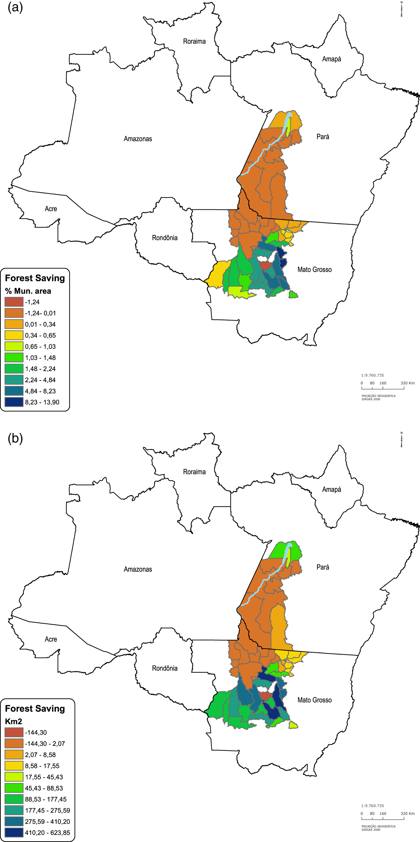
The two panels in figure 4 depict the local-level impact of land use changes on deforestation in each of the 49 municipalities from the Tapajós Basin. Panel A reports this effect as a percentage of the municipal area, whereas panel B reports it in square kilometers. The simulations indicate that the local environmental benefits from the expansion in crop cultivation are concentrated in the state of Mato Grosso.
Forest savings. (a) % of municipal area (b) Square Kilometers.
It is important to note that an investigation of the net effect of changes in land use on deforestation is beyond the scope of this paper. This investigation requires combining the local-level effects of cropland expansion with the spillover effects of cropland expansion to other municipalities discussed elsewhere in the literature (e.g., Lapola et al., Reference Lapola, Schaldach, Alcamo, Bondeau, Koch, Koelking and Priess2010; de Sa et al., Reference de Sa, Palmer and di Falco2013; Richards et al., Reference Richards, Walker and Arima2014).
From a theoretical perspective, it is not simple to determine where these spillover effects might be stronger. Ranching might expand in areas with low land prices, low aptitude for crop cultivation or a lot of idle land. From an empirical perspective, it is difficult to estimate these spillover effects due to the existence of the reflection problem (Manski, Reference Manski1993). Some researchers even argue that this problem cannot be overcome in the absence of clear exogenous variation (Gibbons and Overman, Reference Gibbons and Overman2012). Hence, it is an open question whether spillover effects completely offset the local-level effects estimated in this paper.
Nevertheless, the evidence on the local-level effects of changes in land use deforestation helps to understand the coexistence of large cropland expansions with reduced deforestation in some municipalities from the Brazilian agricultural frontier during the 2000s. This issue seems to be of particular importance in the Tajapós basin since it is located in one of the most important vectors cropland expansion in the country.
6. Robustness
6.1 Initial economic environment
The identification assumption on the estimates from the previous section is that–in the absence of changes in relative prices–changes in deforestation would be similar across municipalities located in the same state and with comparable soy and beef price indexes and initial forest area. However, this might not be true if municipalities with different initial economic conditions present different deforestation trends. For instance, suppose that input prices influence deforestation as in the theoretical model outlined in section 3. To the extent that input prices are converging or diverging across municipalities, deforestation will evolve differentially in municipalities with different initial levels of input prices which would violate the identification assumption. An analogous reasoning can be applied to other initial economic conditions.
The initial deforestation levels included in the baseline specification probably capture many of these differences in the initial economic environment. Nevertheless, it is useful to examine whether the empirical results presented in table 3 are driven by different deforestation trends associated with differences in other initial economic conditions. Table 4 reports the results of regressions that control for different measures of initial economic conditions.
Robustness to initial economic environment

Notes: Each column reports the results of regressing annual deforestation on the soy-to-beef relative price index conditional on soy and beef price indexes and a set of additional covariates. The soy price index is obtained by combining initial soy cultivation with aggregate price variation while the beef price index is obtained combining by initial number of cattle with aggregate price variation. All estimates use data from the 49 municipalities in the Tapajós Basin during the period 2002 to 2012. Observations are weighted by the square root of the municipal area. Standard errors clustered at the municipality level are reported in parentheses. ***p < 0.01 **p < 0.05 *p < 0.1.
Column 1 adds transportation costs interacted with time dummies in the baseline specification. Transportation costs is an index that measures the cost to transport goods to São Paulo in 1995. This variable is constructed by NEMESIS/IPEA. The coefficient on relative prices is negative, statistically significant at the 5 per cent level, and quite close to the one estimated in table 3, column 4.
Column 2 includes a measure of land tenure interacted with time dummies in the baseline specification. This measure is the ratio between the number of farms whose proprietors do not have formal titles and the municipal area. This variable is computed using data from the 1995/1996 Agricultural Census. The coefficient on relative prices is also negative, statistically significant at the 10 per cent level, and quite close to the one estimated in table 3, column 4.
Column 3 adds the ratio between the number of tractors and the municipal area interacted with time dummies in the baseline specification. This variable is also computed using data from the 1995/1996 Agricultural Census. The coefficient on relative prices continue to be negative, statistically significant at the 10 per cent level, and quite close to the one estimated in the previous columns.
Column 4 includes the logarithm of wages interacted with time dummies in the specification from table 3, column 4. This variable is obtained from the 2000 Population Census. The coefficient on relative prices is negative and significant at the 5 per cent level. However, its magnitude increases significantly. The effect is roughly double that of the effects estimated in the previous column.
Column 5 adds all the variables together. Notice that this is a quite demanding specification for the data. A total of 120 parameters and fixed effects are estimated. Nevertheless, the coefficient on relative prices continues to be negative and significant at the 5 per cent level. Moreover, its magnitude is close to the one obtained in column 4.
The overall evidence suggests that, if anything, the baseline empirical specification underestimates the effect of crop-to-beef relative prices on deforestation. It is important to highlight that the measures describing the initial economic environment are not only important by themselves but are also probably correlated with important measures for which there is no data, such as the cost of capital, property rights, and land rents. Thus, the evidence reported in table 4 mitigates the concern that differences in trends drive the empirical results presented in table 3.
6.2 Infrastructure and government policies
Other important concern regarding the estimates in the previous section is whether the results are driven not by relative prices but by concurrent changes in infrastructure and government policies. Because infrastructure and government policies typically evolve continuously while prices changes do not, it is unlikely that omission of measures describing infrastructure and government policies drive the results. However, suppose that the identification of the effect of relative prices is coming only from one change in relative prices. To the extent that this change occurred concurrently with a change in infrastructure or government policies, measures describing infrastructure and government policies might bias the results.
Table 5 investigates this issue. It includes different measures of infrastructure and government policies in the specification from table 3, column 4. Column 1 includes the density of bank branches as an additional covariate. This variable is computed using administrative data from the Brazilian Central Bank. Column 2 adds the density of beneficiaries of the Luz para Todos–a large-scale electrification program implemented in Brazil–as an additional covariate. This variable is computed using administrative data from the Ministry of Mining and Energy. Column 3 includes the density of land reform projects as a covariate. This variable is computed using administrative data from the Ministry of Agriculture. Column 4 adds the share of the municipal area covered by protection areas administered by the federal government as an additional covariate. This variable is constructed using GIS information provided by the Ministry of the Environment. Column 5 includes all controls together.Footnote 4
Robustness to infrastructure and government policies

Notes: Each column reports the results of regressing annual deforestation on the soy-to-beef relative price index conditional on soy and beef price indexes and a set of additional covariates. The soy price index is obtained by combining initial soy cultivation with aggregate price variation while the beef price index is obtained combining by initial number of cattle with aggregate price variation. All estimates use data from the 49 municipalities in the Tapajós Basin during the period 2002 to 2012. Observations are weighted by the square root of the municipal area. Standard errors clustered at the municipality level are reported in parentheses. ***p < 0.01 **p < 0.05 *p < 0.1.
While not exhaustive, the controls described above capture dimensions of infrastructure and government policies that are known to influence deforestation (Andam et al., Reference Andam, Ferraro, Pfaff, Sanchez-Azofeifa and Robalino2008; Assunção and Rocha, Reference Assunção and Rocha2016; Assunção et al., Reference Assunção, Gandour, Rocha and Rocha2013, Reference Assunção, Lipscomb, Mobarak and Szerman2014). Hence, their effect on the results is informative with regard to the possibility that omitted variables drive the results obtained in the previous section. Table 5 suggests that the included measures of infrastructure and government policies do not drive the relationship between relative prices and deforestation. The estimated effects of relative prices are negative, statistically significant at the 10 per cent level and close to the coefficients estimated in table 3.
6.3 Price indexes, weights and standard errors
The results are also robust to changes in the definition of the price index and in weighting procedures. Moreover, the results are robust to allowing spatial correlation in the error term. Online appendix C discusses these robustness tests in detail and presents three tables. Table A1 provides evidence that the results are robust to using a ‘Paasche Price Index’ and to using alternative price indexes that incorporate information on maize production and maize prices. Table A2 provides evidence that neither weighting nor not weighting the observations using the municipal area influences the results. Table A3 provides evidence that inference is robust to allowing the error term to be spatially correlated across municipalities.
7. Conclusion
This paper provides evidence that changes in land use affect deforestation in the Tapajós Basin in Brazil. Using exogenous variation in crop-to-beef relative prices, it is estimated that an increase in relative prices generates an expansion of cropland and a reduction in cattle ranching and deforestation. These effects suggest that changes in land use have important consequences for forest conservation in this region.
A simple economic model is used to rationalize these findings. The model assumes that crop cultivation is more intensive in capital (e.g., tractors, fertilizers) and labor (e.g., tractor operators, agricultural technicians, agronomists) than cattle ranching is. Therefore, input prices will increase if land allocation shifts towards the more input-intensive product (crops) and decrease if it shifts towards the less input-intensive one (cattle). These changes in input prices will affect deforestation because it will influence farmers' choice on whether or not to clear forests. In particular, an increase in input prices will induce low productivity cattle ranchers to leave agriculture, while a decrease in input prices will induce low productivity cattle ranchers to enter the sector. Deforestation will fall in the former scenario and grow in the latter.
The theoretical model and the empirical evidence point out that changes in land use in the direction of input-intensive agriculture (using tractors, fertilizers and so forth) have the potential to generate positive local-level environmental externalities. These results have important implications for environmental and agricultural policies in Brazil. The paper suggests that policies that increase the return from crop cultivation relative to the return from cattle ranching in the Brazilian agricultural frontier will not increase deforestation in the areas directly affected by them. However, it is important to note that negative general equilibrium effects might overcome these positive local-level effects discussed in the paper. Using credible strategies to understand these spillover effects is an important question for future research.
Supplementary material
The supplementary material for this article can be found at https://doi.org/10.1017/S1355770X18000062.
Acknowledgements
I would like to thank Juliano Assuncao, Laisa Rachter, Priscila Souza, Dimitri Szerman for their comments and helpful discussions. I am also thankful to seminar participants at the Climate Policy Initiative, Latin American Meeting of the Econometric Society (LAMES), and the Brazilian Econometric Society Meeting for helpful comments and suggestions. Financial support from the Children‘s Investment Fund Foundation (CIFF) is gratefully acknowledged. All errors are my own.


 Open access