


1. Introduction
Turbulent boundary layers (TBL) have been extensively studied since the seminal work of Prandtl (Prandtl Reference Prandtl1904), due to their theoretical and engineering relevance. Mean and second-order statistics of the velocity field in TBL evolving under nominally zero pressure gradients (ZPG) have been extensively reported in the literature (see reviews by Fernholz & Finley (Reference Fernholz and Finley1996), Klewicki (Reference Klewicki2010) and Smits, McKeon & Marusic (Reference Smits, McKeon and Marusic2011)). However, many flows of practical interest have TBL evolving under pressure gradients, both favourable (FPG) and adverse (APG). The FPG is known to stabilise the boundary layer and can reduce turbulence to the extent of relaminarisation (Narasimha & Sreenivasan Reference Narasimha and Sreenivasan1973; Araya, Castillo & Hussain Reference Araya, Castillo and Hussain2015), whereas APG enhances turbulence and can cause flow separation (Simpson Reference Simpson1989).
Several non-dimensional parameters have been proposed to quantify pressure gradient effects on TBL, based on different length and velocity scales used to normalise the free stream pressure gradient ( ${\textrm d}P_e/{\textrm d}x$
). Some of the popular pressure gradient parameters are the Rotta–Clauser pressure gradient parameter (
${\textrm d}P_e/{\textrm d}x$
). Some of the popular pressure gradient parameters are the Rotta–Clauser pressure gradient parameter ( $\beta$
), acceleration parameter (
$\beta$
), acceleration parameter ( $K$
) and inner-scaled pressure-gradient parameter (
$K$
) and inner-scaled pressure-gradient parameter ( $p_x^+$
), defined as
$p_x^+$
), defined as
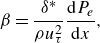 \begin{align} \beta = \frac {\delta ^*}{\rho u_{\tau }^2} \frac {{\textrm d}P_e}{{\textrm d}x}, \end{align}
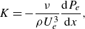 \begin{align} K = - \frac {\nu }{\rho U_e^{3}} \frac {{\textrm d}P_e}{{\textrm d}x}, \end{align}
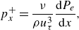 \begin{align} p_x^+ = \frac {\nu }{\rho u_{\tau }^{3}} \frac {{\textrm d}P_e}{{\textrm d}x}, \end{align}
where $\nu$
is the kinematic viscosity,
$\nu$
is the kinematic viscosity, $\rho$
is density,
$\rho$
is density, $\delta ^*$
is the displacement thickness,
$\delta ^*$
is the displacement thickness, $U_e$
is the free stream velocity and
$U_e$
is the free stream velocity and $u_{\tau }$
is the friction velocity defined as
$u_{\tau }$
is the friction velocity defined as $u_{\tau } = \sqrt { \tau _w/\rho }$
. Note that
$u_{\tau } = \sqrt { \tau _w/\rho }$
. Note that $\beta$
and
$\beta$
and $K$
are related as
$K$
are related as $\beta = - K Re_{\delta ^*} (U_e^2/u_{\tau }^2)$
, where
$\beta = - K Re_{\delta ^*} (U_e^2/u_{\tau }^2)$
, where $Re_{\delta ^*}$
is the displacement thickness-based Reynolds number and subscript ‘e’ denotes the value at the edge of the boundary layer.
$Re_{\delta ^*}$
is the displacement thickness-based Reynolds number and subscript ‘e’ denotes the value at the edge of the boundary layer.
There are several past studies on TBL evolving under the influence of pressure gradients, using both experiments (Launder & Jones Reference Launder and Jones1969; Jones & Launder Reference Jones and Launder1972; Skåre & Krogstad Reference Skåre and Krogstad1994; Fernholz & Warnack Reference Fernholz and Finley1998; Warnack & Fernholz Reference Warnack and Fernholz1998; Castillo & George Reference Castillo and George2001; Jones, Marusic & Perry Reference Jones, Marusic and Perry2001; Aubertine & Eaton Reference Aubertine and Eaton2005; Harun et al. Reference Harun, Monty, Mathis and Marusic2013; Knopp et al. Reference Knopp, Reuther, Novara, Schanz, Schülein, Schröder and Kähler2021; Romero et al. Reference Romero, Zimmerman, Philip, White and Klewicki2022) and simulations (Spalart Reference Spalart1986; Skote, Henningson & Henkes Reference Skote, Henningson and Henkes1998; Piomelli, Balaras & Pascarelli Reference Piomelli, Balaras and Pascarelli2000; Lee & Sung Reference Lee and Sung2009; Bobke et al. Reference Bobke, Vinuesa, Örlü and Schlatter2017; Kitsios et al. Reference Kitsios, Sekimoto, Atkinson, Sillero, Borrell, Gungor, Jiménez and Soria2017; Lee Reference Lee2017; Pozuelo et al. Reference Pozuelo, Li, Schlatter and Vinuesa2022), primarily focused on near-equilibrium TBL. Strictly speaking, the boundary layer reaches equilibrium when the mean flow and Reynolds-stress components become independent of the streamwise position, when scaled appropriately with local velocity and length scales (Townsend Reference Townsend1956). However, a less restrictive near-equilibrium condition can be defined when the mean velocity defect is self-similar in the outer region, which is true at high Reynolds number ( $Re$
) (Marusic et al. Reference Marusic, McKeon, Monkewitz, Nagib, Smits and Sreenivasan2010). Townsend (Reference Townsend1956) and Mellor & Gibson (Reference Mellor and Gibson1966) showed that these near-equilibrium conditions can be obtained when
$Re$
) (Marusic et al. Reference Marusic, McKeon, Monkewitz, Nagib, Smits and Sreenivasan2010). Townsend (Reference Townsend1956) and Mellor & Gibson (Reference Mellor and Gibson1966) showed that these near-equilibrium conditions can be obtained when $U_e$
is prescribed by a power law such that
$U_e$
is prescribed by a power law such that $U_e \propto (x - x_0)^m$
, where
$U_e \propto (x - x_0)^m$
, where $x_0$
is a virtual origin and
$x_0$
is a virtual origin and $m$
is the power-law exponent, larger than
$m$
is the power-law exponent, larger than $-1/3$
in order to obtain near-equilibrium conditions. Any high
$-1/3$
in order to obtain near-equilibrium conditions. Any high $Re$
TBL with a constant
$Re$
TBL with a constant $\beta$
(including the ZPG TBL where
$\beta$
(including the ZPG TBL where $\beta = 0$
) is a particular case of near-equilibrium TBL, in which the outer region has a self-similar mean velocity defect (Marusic et al. Reference Marusic, McKeon, Monkewitz, Nagib, Smits and Sreenivasan2010). Some numerical studies on pressure gradient TBL (for example, Yuan & Piomelli (Reference Yuan and Piomelli2014, Reference Yuan and Piomelli2015) and Wu & Piomelli (Reference Wu and Piomelli2018)) have even included the effect of wall roughness in their simulation set-up. The present literature review is not comprehensive as there are several other past studies which have also looked at TBL undergoing separation and reattachment, relaminarisation, unsteady pressure gradients effects, etc. Devenport & Lowe (Reference Devenport and Lowe2022) reviewed recent progress in equilibrium and non-equilibrium TBL. Bobke et al. (Reference Bobke, Vinuesa, Örlü and Schlatter2017) studied history effects in APG TBL using wall-resolved large-eddy simulation (LES). Their simulations of flow over flat plate were designed carefully to induce large region of near-constant
$\beta = 0$
) is a particular case of near-equilibrium TBL, in which the outer region has a self-similar mean velocity defect (Marusic et al. Reference Marusic, McKeon, Monkewitz, Nagib, Smits and Sreenivasan2010). Some numerical studies on pressure gradient TBL (for example, Yuan & Piomelli (Reference Yuan and Piomelli2014, Reference Yuan and Piomelli2015) and Wu & Piomelli (Reference Wu and Piomelli2018)) have even included the effect of wall roughness in their simulation set-up. The present literature review is not comprehensive as there are several other past studies which have also looked at TBL undergoing separation and reattachment, relaminarisation, unsteady pressure gradients effects, etc. Devenport & Lowe (Reference Devenport and Lowe2022) reviewed recent progress in equilibrium and non-equilibrium TBL. Bobke et al. (Reference Bobke, Vinuesa, Örlü and Schlatter2017) studied history effects in APG TBL using wall-resolved large-eddy simulation (LES). Their simulations of flow over flat plate were designed carefully to induce large region of near-constant $\beta$
. They also simulated TBL with non-constant
$\beta$
. They also simulated TBL with non-constant $\beta$
and performed comparative studies to quantify history effects on the evolution of APG TBL. They concluded that
$\beta$
and performed comparative studies to quantify history effects on the evolution of APG TBL. They concluded that $\beta$
and the friction-based Reynolds number (
$\beta$
and the friction-based Reynolds number ( $Re_{\tau }$
) are insufficient to fully characterise the state of a general pressure gradient TBL. Recently, Pozuelo et al. (Reference Pozuelo, Li, Schlatter and Vinuesa2022) reported wall-resolved LES results of APG TBL where
$Re_{\tau }$
) are insufficient to fully characterise the state of a general pressure gradient TBL. Recently, Pozuelo et al. (Reference Pozuelo, Li, Schlatter and Vinuesa2022) reported wall-resolved LES results of APG TBL where $\beta$
was held approximately constant at 1.4 up to a momentum-thickness-based Reynolds number
$\beta$
was held approximately constant at 1.4 up to a momentum-thickness-based Reynolds number $Re_{\theta } \approx 8700$
. Their simulations are the highest
$Re_{\theta } \approx 8700$
. Their simulations are the highest $Re$
reported until date for near-equilibrium APG TBL.
$Re$
reported until date for near-equilibrium APG TBL.
The analysis of non-equilibrium TBL poses many challenges. Several length and velocity scales have been proposed for the inner and outer regions of TBL evolving under pressure gradients. Maciel et al. (Reference Maciel, Wei, Gungor and Simens2018) proposed a consistent framework to analyse APG TBL and identified three parameters to characterise APG TBL. These parameters, namely, the pressure gradient parameter, Reynolds number and the inertial parameter were obtained using scaling analysis of the governing equations. They also discussed how their general parameters relate to commonly used quantities like $\beta$
and
$\beta$
and $Re_{\tau }$
and the Zagarola–Smits velocity scale (Zagarola & Smits Reference Zagarola and Smits1998a
,
Reference Zagarola and Smitsb
).
$Re_{\tau }$
and the Zagarola–Smits velocity scale (Zagarola & Smits Reference Zagarola and Smits1998a
,
Reference Zagarola and Smitsb
).
Recently, Volino (Reference Volino2020a
) conducted experiments to study TBL subject to pressure gradients. Their experiments were unique in the sense that an initial equilibrium TBL at ZPG is subjected to FPG, then recovered to ZPG, followed by APG. The desired pressure gradient was applied using a ramp as a top wall, which essentially sets $K$
to a constant value in different regions of the ramp. Here
$K$
to a constant value in different regions of the ramp. Here $K$
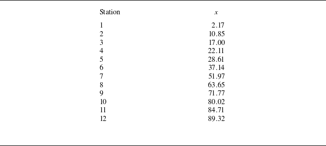
was held constant and mild enough to avoid relaminarisation or separation. The mean velocity and turbulence statistics along with the integral quantities and wall shear determined from them were documented. In particular, profile measurements were reported at 12 streamwise stations (Station 1–12) in their set-up where Station 1, 6 and 9 were located at the beginning of FPG, ZPG recovery and APG regions, respectively. They performed experiments at eight different physical conditions by setting
$K$
was held constant and mild enough to avoid relaminarisation or separation. The mean velocity and turbulence statistics along with the integral quantities and wall shear determined from them were documented. In particular, profile measurements were reported at 12 streamwise stations (Station 1–12) in their set-up where Station 1, 6 and 9 were located at the beginning of FPG, ZPG recovery and APG regions, respectively. They performed experiments at eight different physical conditions by setting $U_e$
at the inflow and
$U_e$
at the inflow and $K$
in the FPG, APG region using different ramps. Their Case 4, where
$K$
in the FPG, APG region using different ramps. Their Case 4, where $U_e = 1\,\rm ms^{-1}$
at the inflow and
$U_e = 1\,\rm ms^{-1}$
at the inflow and $K=5 \times 10^{-7}$
in the FPG region is taken as the reference for the present work. The
$K=5 \times 10^{-7}$
in the FPG region is taken as the reference for the present work. The $Re_{\theta }$
for this case varies from 1578 at Station 1 to 3846 at Station 6. The present gradient causes the boundary layer to become thin in the FPG region and thick in the APG region. Capturing thin boundary layer in FPG region demands fine grid resolution, and thick boundary layer in APG region requires bigger spanwise domain. This particular case was chosen due to its unique combination of pressure gradient and
$Re_{\theta }$
for this case varies from 1578 at Station 1 to 3846 at Station 6. The present gradient causes the boundary layer to become thin in the FPG region and thick in the APG region. Capturing thin boundary layer in FPG region demands fine grid resolution, and thick boundary layer in APG region requires bigger spanwise domain. This particular case was chosen due to its unique combination of pressure gradient and $Re$
range. The pressure gradient for the case is moderate and its
$Re$
range. The pressure gradient for the case is moderate and its $Re_{\tau }$
ranges from 570–1072 (table 1 of Volino Reference Volino2020a
), which is moderately high. Higher pressure gradient and
$Re_{\tau }$
ranges from 570–1072 (table 1 of Volino Reference Volino2020a
), which is moderately high. Higher pressure gradient and $Re_{\tau }$
will significantly increase the computational cost.
$Re_{\tau }$
will significantly increase the computational cost.
The main goals of the present work are to accurately simulate the reference experiment (Case 4 of Volino Reference Volino2020a
) and analyse the results to understand the behaviour of TBL in non-equilibrium conditions. Simulation of such non-equilibrium TBL has several challenges. First of all, the rapid thinning and thickening of the boundary layer thickness requires careful design of the computational grid in order to ensure adequate resolution of the inner layer. The boundary layer becomes very thin in the FPG region, which is the most critical region for the present case as any error in this region can cause large mismatch in rest of the flow field downstream. Second, accurate prediction of turbulent stresses and skin-friction at high $Re$
is demanding. Third, the domain size and boundary conditions should be such that the experimental conditions are closely matched without compromising accuracy.
$Re$
is demanding. Third, the domain size and boundary conditions should be such that the experimental conditions are closely matched without compromising accuracy.
In this work, wall-resolved LES of non-equilibrium TBL is performed, closely matching the set-up of the reference experiment. The present simulations are the first of its kind where the entire streamwise evolution of the non-equilibrium TBL in the reference experiment is captured. The rest of the paper is organised as follows. The simulation details are described in 2. Results are described in 3. The present problem is analysed in 4 where the scaling behaviour, the modelling implications and the response of TBL to non-equilibrium conditions are discussed. The key findings of the present work are summarised in 5.
2. Simulation details
2.1. Numerical algorithm
In LES, large scales are resolved by the spatially filtered Navier–Stokes equations and the effect of small scales is modelled. The spatially filtered incompressible Navier–Stokes equations are
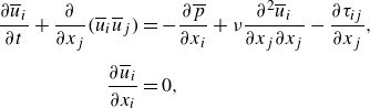 \begin{equation} \begin{aligned} \frac {\partial {\overline {u}_i}}{\partial {t}} + \frac {\partial {}}{\partial {x_{j}}}(\overline {u}_{i}\overline {u}_{j}) & = -\frac {\partial {\overline {p}}}{\partial {x_i}} + \nu \frac {\partial ^2{\overline {u}_i}}{\partial {x_j}\partial {x_j}} - \frac {\partial {\tau _{ij}}}{\partial {x_j}},\\[4pt] \frac {\partial {\overline {u}_i}}{\partial {x_i}} & = 0, \end{aligned} \end{equation}
where $u_i$
is the velocity,
$u_i$
is the velocity, $p$
is the pressure and
$p$
is the pressure and $\nu$
is the kinematic viscosity. The overbar
$\nu$
is the kinematic viscosity. The overbar $\overline {(\cdot )}$
denotes spatial filtering and
$\overline {(\cdot )}$
denotes spatial filtering and $\tau _{ij}=\overline {u_iu_j}-\overline {u}_i\overline {u}_j$
is the subgrid stress. The subgrid stress is modelled using the dynamic Smagorinsky Model (Germano et al. Reference Germano, Piomelli, Moin and Cabot1991; Lilly Reference Lilly1992). The Lagrangian time scale is dynamically computed based on surrogate correlation of the Germano-identity error (Park & Mahesh Reference Park and Mahesh2009). This approach, extended to unstructured grids, has shown good performance for a variety of flows including plane channel flow, circular cylinder and flow past a marine propeller in crashback (Verma & Mahesh Reference Verma and Mahesh2012).
$\tau _{ij}=\overline {u_iu_j}-\overline {u}_i\overline {u}_j$
is the subgrid stress. The subgrid stress is modelled using the dynamic Smagorinsky Model (Germano et al. Reference Germano, Piomelli, Moin and Cabot1991; Lilly Reference Lilly1992). The Lagrangian time scale is dynamically computed based on surrogate correlation of the Germano-identity error (Park & Mahesh Reference Park and Mahesh2009). This approach, extended to unstructured grids, has shown good performance for a variety of flows including plane channel flow, circular cylinder and flow past a marine propeller in crashback (Verma & Mahesh Reference Verma and Mahesh2012).
Equation (2.1) is solved using a numerical method developed by Mahesh, Constantinescu & Moin (Reference Mahesh, Constantinescu and Moin2004) for incompressible flows on unstructured grids. The algorithm is derived to be robust without numerical dissipation. It is a finite volume method where the Cartesian velocities and pressure are stored at the centroids of the cells and the face normal velocities are stored independently at the centroids of the faces. A predictor–corrector approach is used. The predicted velocities at the control volume centroids are first obtained and then interpolated to obtain the face normal velocities. The predicted face normal velocity is projected so that the continuity equation in (2.1) is discretely satisfied. This yields a Poisson equation for pressure which is solved iteratively using a multigrid approach. The pressure field is used to update the Cartesian control volume velocities using a least-square formulation. Time advancement is performed using an implicit Crank–Nicolson scheme. The algorithm has been validated for a variety of problems over a range of $Re$
including flow over axisymmetric hull (Kumar & Mahesh Reference Kumar and Mahesh2018).
$Re$
including flow over axisymmetric hull (Kumar & Mahesh Reference Kumar and Mahesh2018).
2.2. Computational domain and boundary conditions
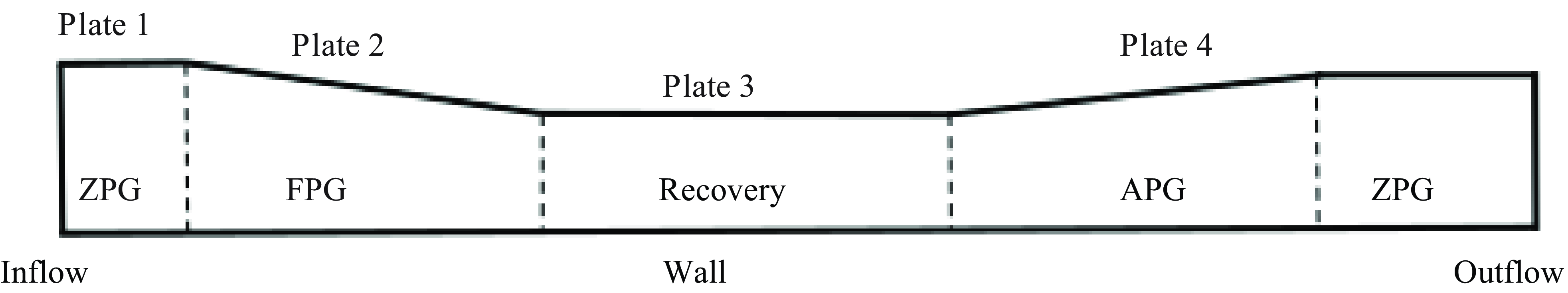
Figure 1 shows a schematic of the computational domain, which is based on the experimental set-up of Volino (Reference Volino2020a
). The reference coordinate system is chosen such that the streamwise, wall-normal and spanwise coordinates are $x$
,
$x$
, $y$
and
$y$
and $z$
, respectively, and the origin is located on the bottom wall (
$z$
, respectively, and the origin is located on the bottom wall ( $y=0$
plane) at the inflow plane (
$y=0$
plane) at the inflow plane ( $x=0$
plane). The flow is in the direction of positive
$x=0$
plane). The flow is in the direction of positive $x$
. In the reference experiment, the top wall is comprised of four plates that were adjusted to prescribe a desired
$x$
. In the reference experiment, the top wall is comprised of four plates that were adjusted to prescribe a desired $K$
in different regions. In the computational domain, those plates are geometrically identical except for Plate 1 which is made shorter, the reason for that will be discussed later. The test section in the reference experiment ends at the end of Plate 4. However in the computational domain, a horizontal wall (Plate 5) is appended at the end of Plate 4 to ensure minimal effect of the outflow boundary condition.
$K$
in different regions. In the computational domain, those plates are geometrically identical except for Plate 1 which is made shorter, the reason for that will be discussed later. The test section in the reference experiment ends at the end of Plate 4. However in the computational domain, a horizontal wall (Plate 5) is appended at the end of Plate 4 to ensure minimal effect of the outflow boundary condition.
A schematic of the computational domain in $xy$
plane showing ZPG, FPG, recovery and APG regions. Plates 2–4 at the top boundary correspond to those used in the reference experiments (Volino Reference Volino2020a
) to impose streamwise varying pressure gradients.
$xy$
plane showing ZPG, FPG, recovery and APG regions. Plates 2–4 at the top boundary correspond to those used in the reference experiments (Volino Reference Volino2020a
) to impose streamwise varying pressure gradients.
The boundary layer thickness ( $\delta$
) and
$\delta$
) and $U_e$
is nominally unity at the inflow plane. The inflow plane (
$U_e$
is nominally unity at the inflow plane. The inflow plane ( $x = 0$
) is located
$x = 0$
) is located $5.46$
units upstream of the beginning of Plate 2. The outflow plane (
$5.46$
units upstream of the beginning of Plate 2. The outflow plane ( $x = 109.89$
) is
$x = 109.89$
) is $7.28$
units downstream of the end of Plate 4. Plates 1 and 5 are parallel to the bottom wall and situated at a wall-normal distance of 7.51 and 7.09 units, respectively, from the bottom wall. Additional details of the computational domain are listed in table 1. The location of the streamwise stations corresponding to the measurement stations in the reference experiment is listed in table 2.
$7.28$
units downstream of the end of Plate 4. Plates 1 and 5 are parallel to the bottom wall and situated at a wall-normal distance of 7.51 and 7.09 units, respectively, from the bottom wall. Additional details of the computational domain are listed in table 1. The location of the streamwise stations corresponding to the measurement stations in the reference experiment is listed in table 2.
Details of the computational domain in grid units. Note that $\delta =1$
at the inflow is taken as the reference length for the domain.
$\delta =1$
at the inflow is taken as the reference length for the domain.
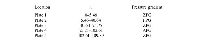
Streamwise coordinate of Stations 1–12 where the profiles are compared with the reference experimental data of Volino (Reference Volino2020a ).
Periodic boundary conditions are applied in the spanwise direction and convective boundary conditions are prescribed at the outflow. Bottom and top boundaries are prescribed as a no-slip condition. A ZPG TBL of desired parameters is prescribed at the inflow plane. This TBL is generated in an auxiliary simulation using the recycle–rescale method of Lund, Wu & Squires (Reference Lund, Wu and Squires1998) extended to unstructured grids employing the numerical method discussed in 2.1. The inflow generation method is described and validated for a range of $Re_{\theta }$
in Appendix A.
$Re_{\theta }$
in Appendix A.
The bottom wall is tripped far away from the test section in the reference experiment. The use of the auxiliary simulation to generate turbulent inflow enables drastic reduction in the computational cost by reducing the TBL development region in the present set-up while ensuring equilibrium TBL before the start of FPG region. The decision to place the inflow and outflow boundaries as described earlier is based on the prior experience of the authors in simulating spatially developing TBL. Simulations were performed for a domain with a spanwise length of 3 units initially (not shown here). But owing to the rapid growth of TBL thickness in the APG region, the simulations were repeated for a domain with double the spanwise length (6 units) to ensure minimal domain effects. The difference in flow field was minimal between the two domains (see Appendix B).
The grid generation for the present flow problem is challenging due to rapidly varying TBL thickness and strong gradients. The nominally ZPG TBL undergoes a region of FPG, ZPG and APG consequently, which requires a carefully designed non-uniform grid in streamwise and wall-normal directions. The computational grid of the main simulation consists of $395.2\times 10^6$
(
$395.2\times 10^6$
( $N_x \times N_y \times N_z = 2470 \times 400 \times 400$
) hexahedral control volumes. The five segments of the bottom wall shown in figure 1 contain 120, 800, 800, 650 and 100 cells in that order. The authors performed simulations with several coarser grids to arrive at the final grid. The grid is uniform in the
$N_x \times N_y \times N_z = 2470 \times 400 \times 400$
) hexahedral control volumes. The five segments of the bottom wall shown in figure 1 contain 120, 800, 800, 650 and 100 cells in that order. The authors performed simulations with several coarser grids to arrive at the final grid. The grid is uniform in the $z$
direction only. The first off-wall cell height is
$z$
direction only. The first off-wall cell height is $0.0005$
throughout the domain at the bottom wall. No attempt was made to resolve the top wall. The first off-wall cell height is
$0.0005$
throughout the domain at the bottom wall. No attempt was made to resolve the top wall. The first off-wall cell height is ${\sim}0.1$
at the top wall. The grid was generated such that the computational cells are normal to the top wall for at least the first few cells. The grid progressively becomes finer in
${\sim}0.1$
at the top wall. The grid was generated such that the computational cells are normal to the top wall for at least the first few cells. The grid progressively becomes finer in $x$
going from the inflow to the FPG region, becomes coarser slowly until the beginning of the APG region, after which it maintains uniformity in
$x$
going from the inflow to the FPG region, becomes coarser slowly until the beginning of the APG region, after which it maintains uniformity in $x$
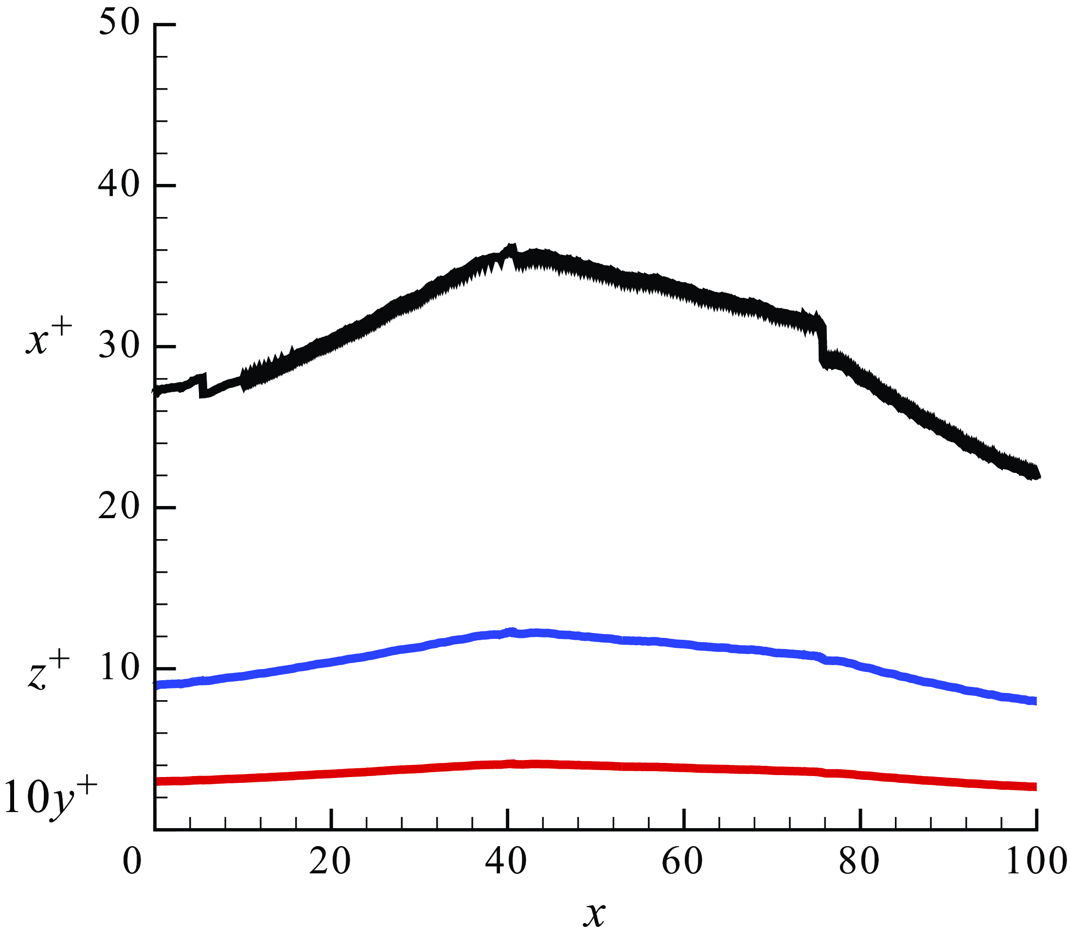
direction for the entire APG region. Subsequently, the grid is coarsened slowly towards the outflow plane. Figure 2 shows the grid resolution in viscous units in the domain at the first cell height. The wall-normal and spanwise resolution remains below 0.4 and 12, respectively, throughout the domain. The streamwise grid resolution stays below 36 and 30 in the FPG and APG regions, respectively. The entire grid was partitioned over
$x$
direction for the entire APG region. Subsequently, the grid is coarsened slowly towards the outflow plane. Figure 2 shows the grid resolution in viscous units in the domain at the first cell height. The wall-normal and spanwise resolution remains below 0.4 and 12, respectively, throughout the domain. The streamwise grid resolution stays below 36 and 30 in the FPG and APG regions, respectively. The entire grid was partitioned over $5280$
processors and the simulations were performed with a time step of
$5280$
processors and the simulations were performed with a time step of $0.001$
unit. The flow field statistics were computed for over one flow through time, after the simulations were performed for at least two flow-through times to discard transients.
$0.001$
unit. The flow field statistics were computed for over one flow through time, after the simulations were performed for at least two flow-through times to discard transients.
Grid resolution in viscous units at the first off-wall cell height.
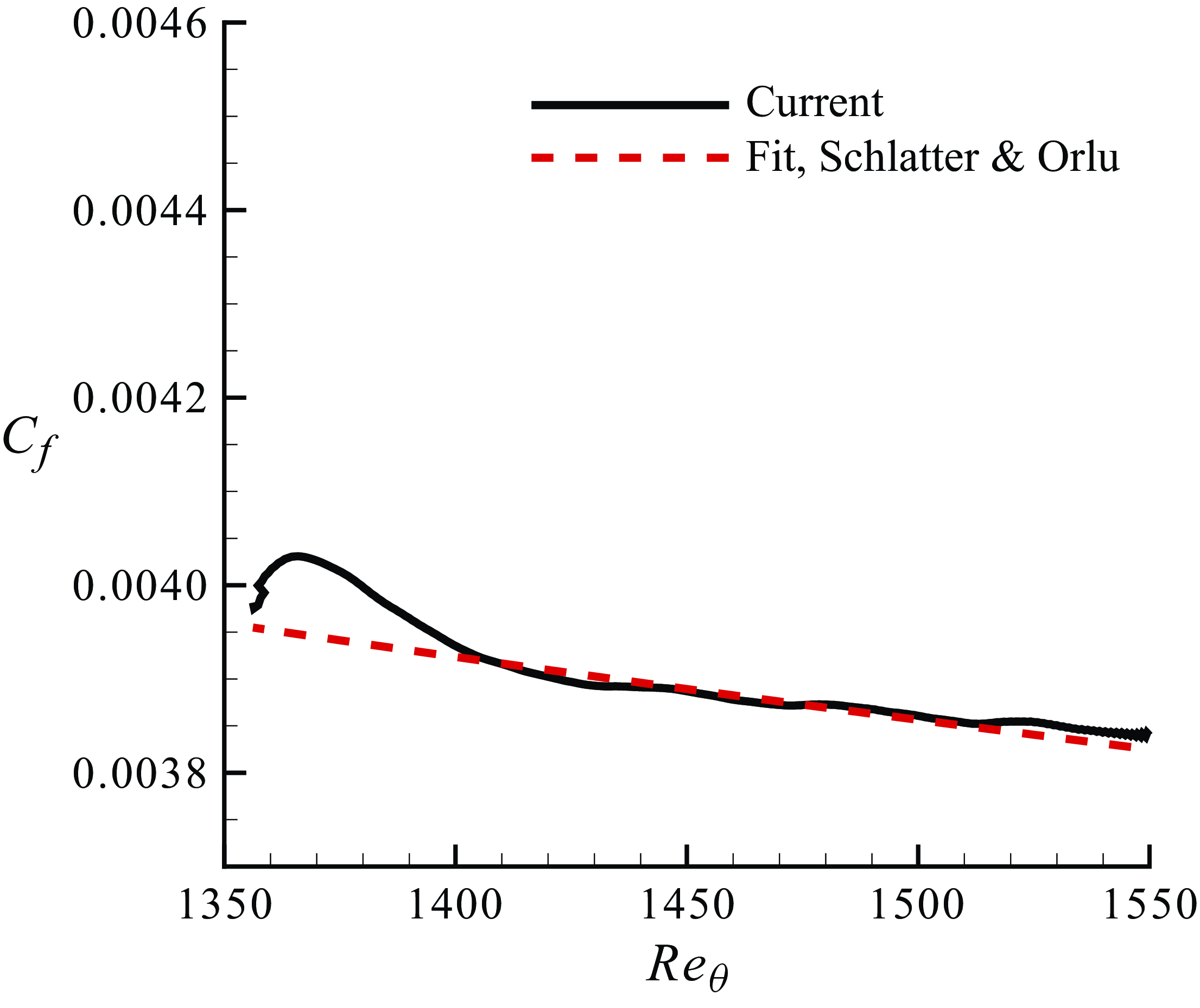
Here $C_f$
compared with the correlation of Schlatter & Örlü (Reference Schlatter and Örlü2010).
$C_f$
compared with the correlation of Schlatter & Örlü (Reference Schlatter and Örlü2010).
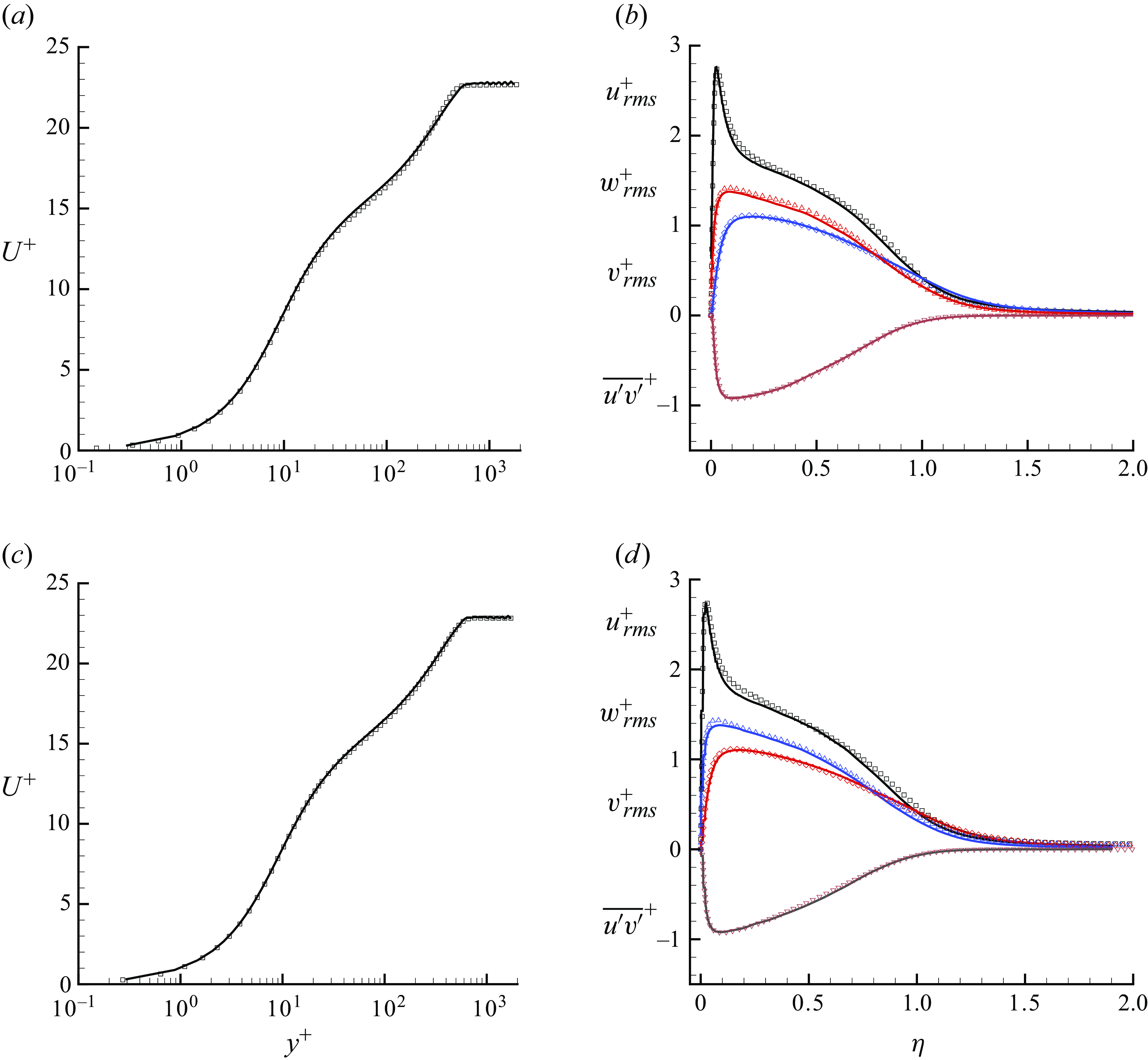
Mean and second-order statistics at $Re_{\theta } = 1420$
(
$Re_{\theta } = 1420$
( $a,b$
) and 1551 (
$a,b$
) and 1551 ( $c,d$
). Symbols are DNS from Schlatter & Örlü (Reference Schlatter and Örlü2010) (a,b) and Jiménez et al. (Reference Jiménez, Hoyas, Simens and Mizuno2010) (c,d).
$c,d$
). Symbols are DNS from Schlatter & Örlü (Reference Schlatter and Örlü2010) (a,b) and Jiménez et al. (Reference Jiménez, Hoyas, Simens and Mizuno2010) (c,d).
2.3. Inflow generation
An auxiliary LES employing the method described in the Appendix A is performed to obtain a turbulent inflow at $Re_{\theta } = 1435$
and
$Re_{\theta } = 1435$
and $\delta \approx 1$
. The computational domain of the simulation consists of a box of dimension
$\delta \approx 1$
. The computational domain of the simulation consists of a box of dimension $100 \theta _i \times 30 \theta _i \times 60 \theta _i$
in the
$100 \theta _i \times 30 \theta _i \times 60 \theta _i$
in the $x$
,
$x$
, $y$
and
$y$
and $z$
directions, respectively, where
$z$
directions, respectively, where $\theta _i$
is the momentum thickness at the inflow plane. The values of
$\theta _i$
is the momentum thickness at the inflow plane. The values of $\theta _i$
and
$\theta _i$
and $Re_{\theta _i}$
are set to
$Re_{\theta _i}$
are set to $0.1$
and
$0.1$
and $1342$
, respectively. These values are chosen so that the target plane where
$1342$
, respectively. These values are chosen so that the target plane where $Re_{\theta } = 1435$
stays sufficiently away from the inflow and outflow boundaries. The grid consists of 300, 200 and 400 cells in the
$Re_{\theta } = 1435$
stays sufficiently away from the inflow and outflow boundaries. The grid consists of 300, 200 and 400 cells in the $x$
,
$x$
, $y$
and
$y$
and $z$
directions. The grid is uniform in
$z$
directions. The grid is uniform in $x$
and
$x$
and $z$
with a clustering in
$z$
with a clustering in $y$
with
$y$
with $1 \,\%$
growth to ensure adequate near-wall resolution. Figure 3 shows the comparison of
$1 \,\%$
growth to ensure adequate near-wall resolution. Figure 3 shows the comparison of $C_f$
with the correlation of Schlatter & Örlü (Reference Schlatter and Örlü2010) showing good agreement away from the inflow. Two profiles are extracted and compared with the direct numerical simulation (DNS) data at
$C_f$
with the correlation of Schlatter & Örlü (Reference Schlatter and Örlü2010) showing good agreement away from the inflow. Two profiles are extracted and compared with the direct numerical simulation (DNS) data at $Re_{\theta }=1420$
(Schlatter & Örlü Reference Schlatter and Örlü2010), and
$Re_{\theta }=1420$
(Schlatter & Örlü Reference Schlatter and Örlü2010), and $Re_{\theta }=1551$
(Jiménez et al. Reference Jiménez, Hoyas, Simens and Mizuno2010) in figure 4. Note that throughout this work,
$Re_{\theta }=1551$
(Jiménez et al. Reference Jiménez, Hoyas, Simens and Mizuno2010) in figure 4. Note that throughout this work, $\eta = y/\delta$
, where
$\eta = y/\delta$
, where $\delta$
is the local boundary layer thickness defined as the wall-normal distance where the mean streamwise velocity reaches
$\delta$
is the local boundary layer thickness defined as the wall-normal distance where the mean streamwise velocity reaches $99 \,\%$
of its local free stream value. The results show very good agreement with the reference data. The grid resolution at these two stations is listed in table 3.
$99 \,\%$
of its local free stream value. The results show very good agreement with the reference data. The grid resolution at these two stations is listed in table 3.
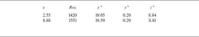
Grid resolution in wall units at different streamwise stations of the auxiliary simulation.
The flow field at the station where $Re_{\theta } = 1435$
is stored at each time step and interpolated on the inflow plane of the main simulation. Note that the spanwise length of the auxiliary simulation and the computational time step match that of the main simulation. But the wall-normal extent of the main simulation is larger than that of the auxiliary simulation. So the velocity field is extrapolated to free stream for
$Re_{\theta } = 1435$
is stored at each time step and interpolated on the inflow plane of the main simulation. Note that the spanwise length of the auxiliary simulation and the computational time step match that of the main simulation. But the wall-normal extent of the main simulation is larger than that of the auxiliary simulation. So the velocity field is extrapolated to free stream for $y \gt 30 \theta _i$
.
$y \gt 30 \theta _i$
.
As mentioned earlier, the top wall is prescribed a no-slip boundary condition. In the reference experiments, the boundary layer was only tripped at the bottom wall where all the measurements where conducted. Hence, no attempt was made to prescribe a TBL at the top wall in the present set-up. It will be shown later that the present set-up was able to accurately simulate the physical conditions of the reference experiments.
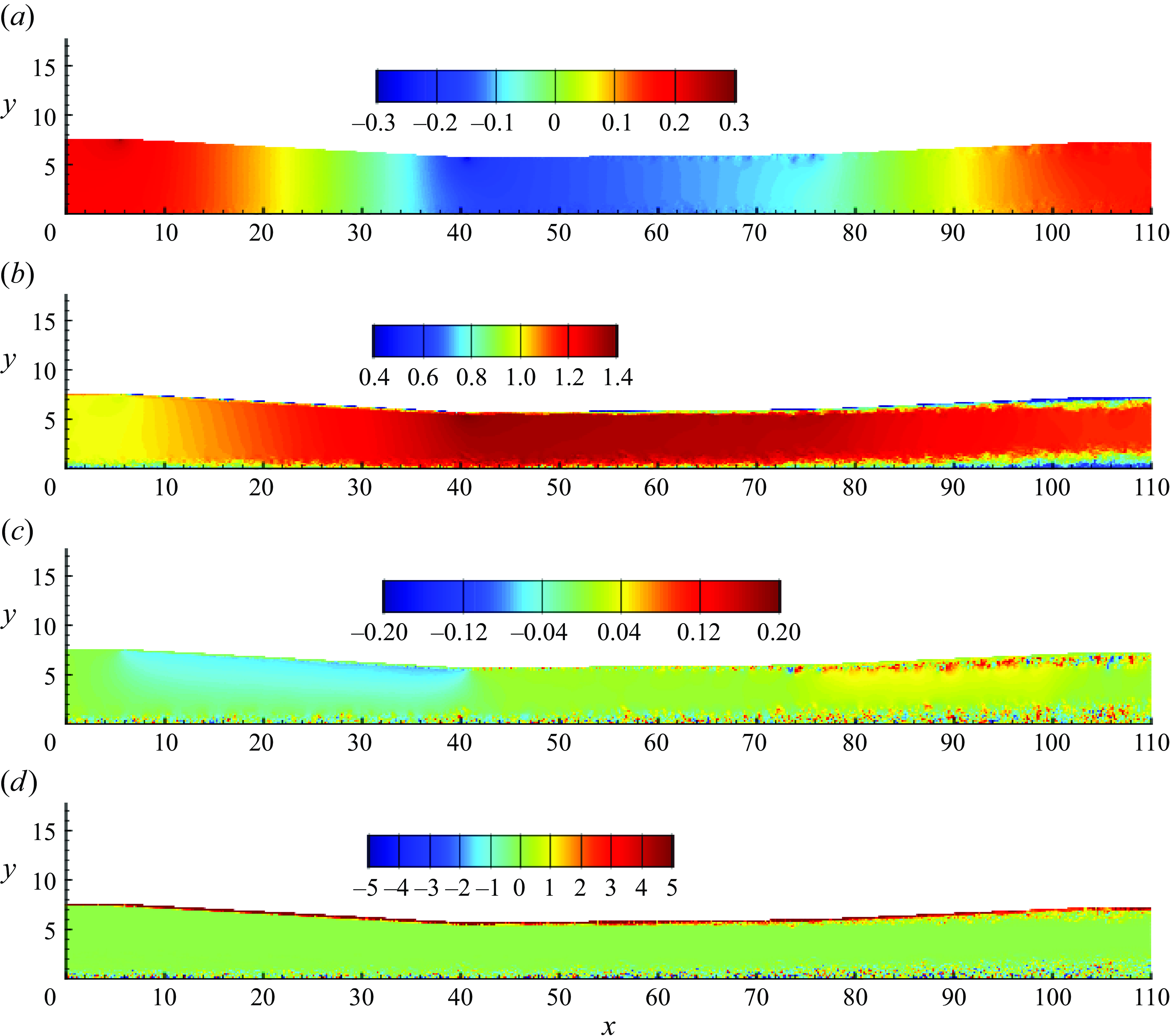
Instantaneous pressure $(a)$
, streamwise velocity
$(a)$
, streamwise velocity $(b)$
, wall-normal velocity
$(b)$
, wall-normal velocity $(c)$
and spanwise vorticity
$(c)$
and spanwise vorticity $(d)$
in
$(d)$
in $xy$
plane. The quantities are normalised with the free stream velocity and boundary layer thickness at the inflow plane.
$xy$
plane. The quantities are normalised with the free stream velocity and boundary layer thickness at the inflow plane.
3. Results
3.1. Instantaneous flow field
Figure 5 shows contour plots of pressure, streamwise velocity, wall-normal velocity and spanwise vorticity fields in the $xy$
plane. The pressure field shows rapid variation throughout the domain. It first rapidly decreases in the FPG region, followed by nearly constant value in the recovery zone and subsequently, increasing rapidly in the APG region. Such rapid variation in pressure causes rapid change in the thickness of the incoming TBL as it passes through the domain, as evident from the streamwise velocity field (figure 5
$xy$
plane. The pressure field shows rapid variation throughout the domain. It first rapidly decreases in the FPG region, followed by nearly constant value in the recovery zone and subsequently, increasing rapidly in the APG region. Such rapid variation in pressure causes rapid change in the thickness of the incoming TBL as it passes through the domain, as evident from the streamwise velocity field (figure 5 $b$
). The grid is designed to appropriately resolve the TBL of the bottom wall. However, a boundary layer can also be observed on the top wall as well in figure 5
$b$
). The grid is designed to appropriately resolve the TBL of the bottom wall. However, a boundary layer can also be observed on the top wall as well in figure 5 $(b{-}d)$
. Note that the top wall in the reference experiments was intended to prescribe a desired external pressure gradient only and not tripped. Moreover, no attempt was made to characterise the top wall boundary layer. Hence, the simulation set-up did not prescribe any boundary layer on the top wall. However, owing to the no slip condition on the top wall, it is natural to expect it to have a boundary layer development on its own, which ends up growing rapidly and likely turning turbulent in the APG region. At this point, it is not clear how significantly the top wall boundary layer affects the bottom wall TBL. However, it is likely that its effect is negligible in most of the domain. As it will shown later, the results of the TBL at the bottom wall match well with the reference data, confirming that the effect of the top wall boundary layer is minimal. As one would expect, the spanwise vorticity is confined in the boundary layer region of the walls.
$(b{-}d)$
. Note that the top wall in the reference experiments was intended to prescribe a desired external pressure gradient only and not tripped. Moreover, no attempt was made to characterise the top wall boundary layer. Hence, the simulation set-up did not prescribe any boundary layer on the top wall. However, owing to the no slip condition on the top wall, it is natural to expect it to have a boundary layer development on its own, which ends up growing rapidly and likely turning turbulent in the APG region. At this point, it is not clear how significantly the top wall boundary layer affects the bottom wall TBL. However, it is likely that its effect is negligible in most of the domain. As it will shown later, the results of the TBL at the bottom wall match well with the reference data, confirming that the effect of the top wall boundary layer is minimal. As one would expect, the spanwise vorticity is confined in the boundary layer region of the walls.
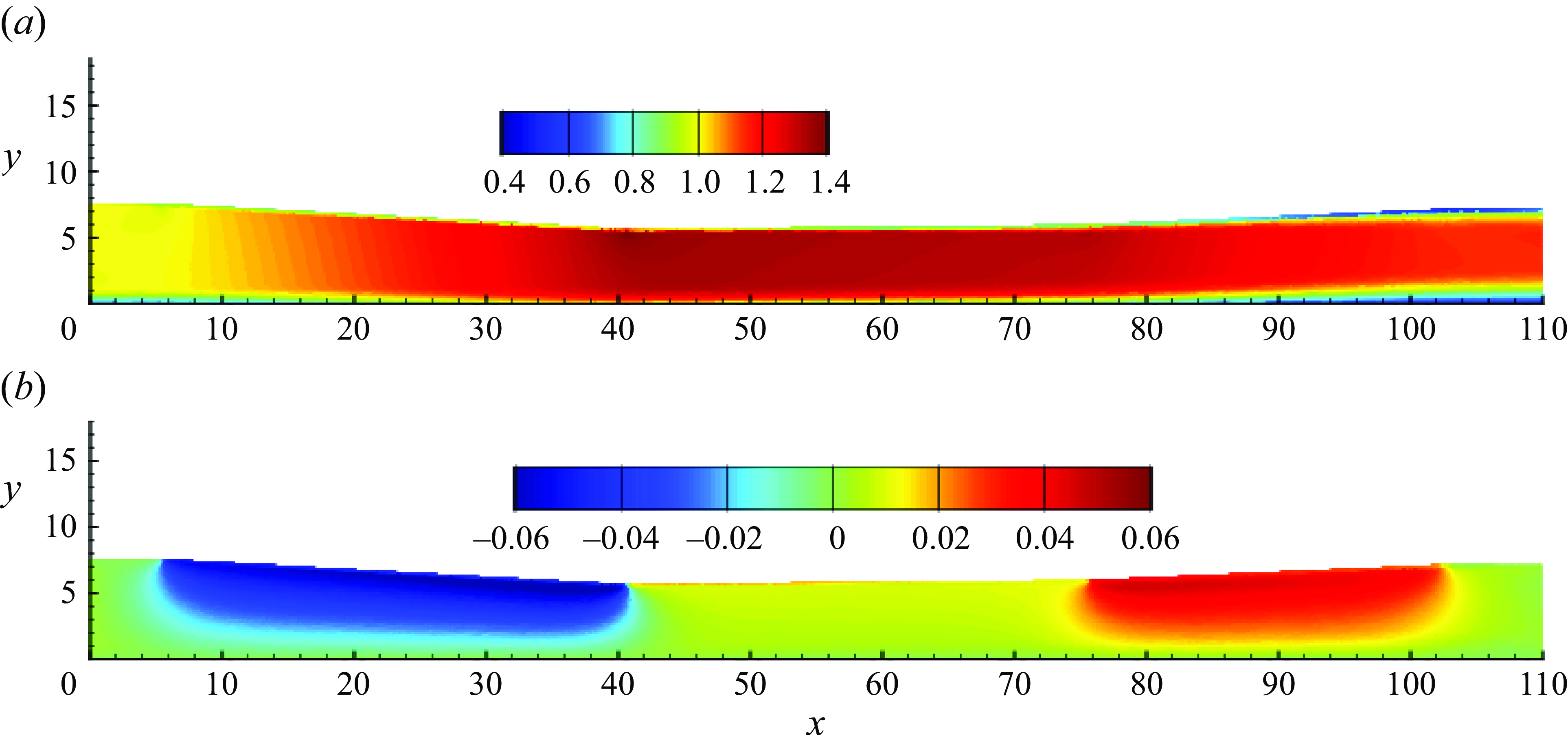
Mean streamwise $(a)$
and wall-normal
$(a)$
and wall-normal $(b)$
velocity fields in
$(b)$
velocity fields in $xy$
plane. The quantities are normalised with the free stream velocity and boundary layer thickness at the inflow plane.
$xy$
plane. The quantities are normalised with the free stream velocity and boundary layer thickness at the inflow plane.
3.2. Mean flow field
The mean flow field is shown in figure 6 for streamwise and wall-normal components of velocity. The rapidly varying boundary layer thickness is evident on the bottom wall throughout the domain. The top wall has negligible boundary layer thickness until the beginning of APG region. Due to APG, the boundary layer thickness on the top wall grows rapidly and becomes comparable to that of the bottom wall towards the end of the flow domain. The streamwise gradient of $U$
should be equal to the negative of wall-normal gradient of
$U$
should be equal to the negative of wall-normal gradient of $V$
to satisfy mass continuity. Hence, the region of accelerating free stream shows reduction
$V$
to satisfy mass continuity. Hence, the region of accelerating free stream shows reduction $V$
away from the wall and vice versa. The recovery region on the other hand shows constant
$V$
away from the wall and vice versa. The recovery region on the other hand shows constant $V$
outside TBL as expected from a ZPG region.
$V$
outside TBL as expected from a ZPG region.
3.3. Comparison with experiments
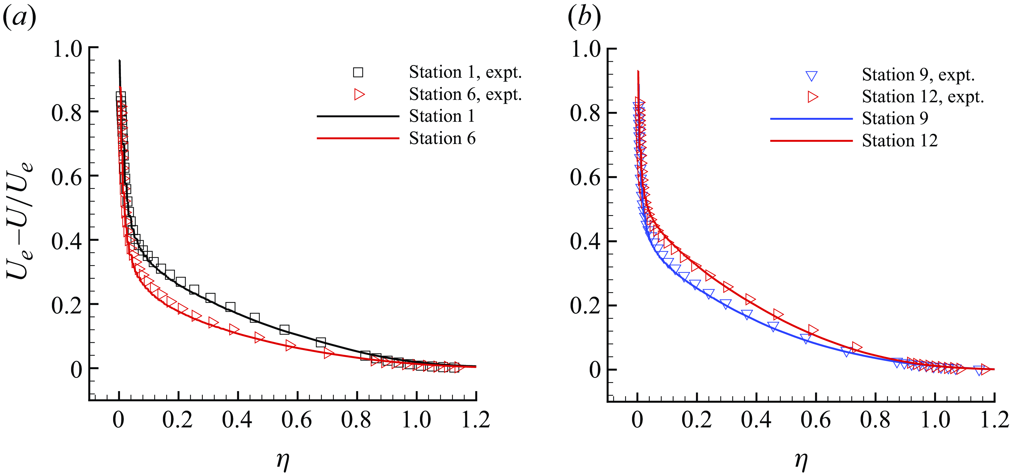
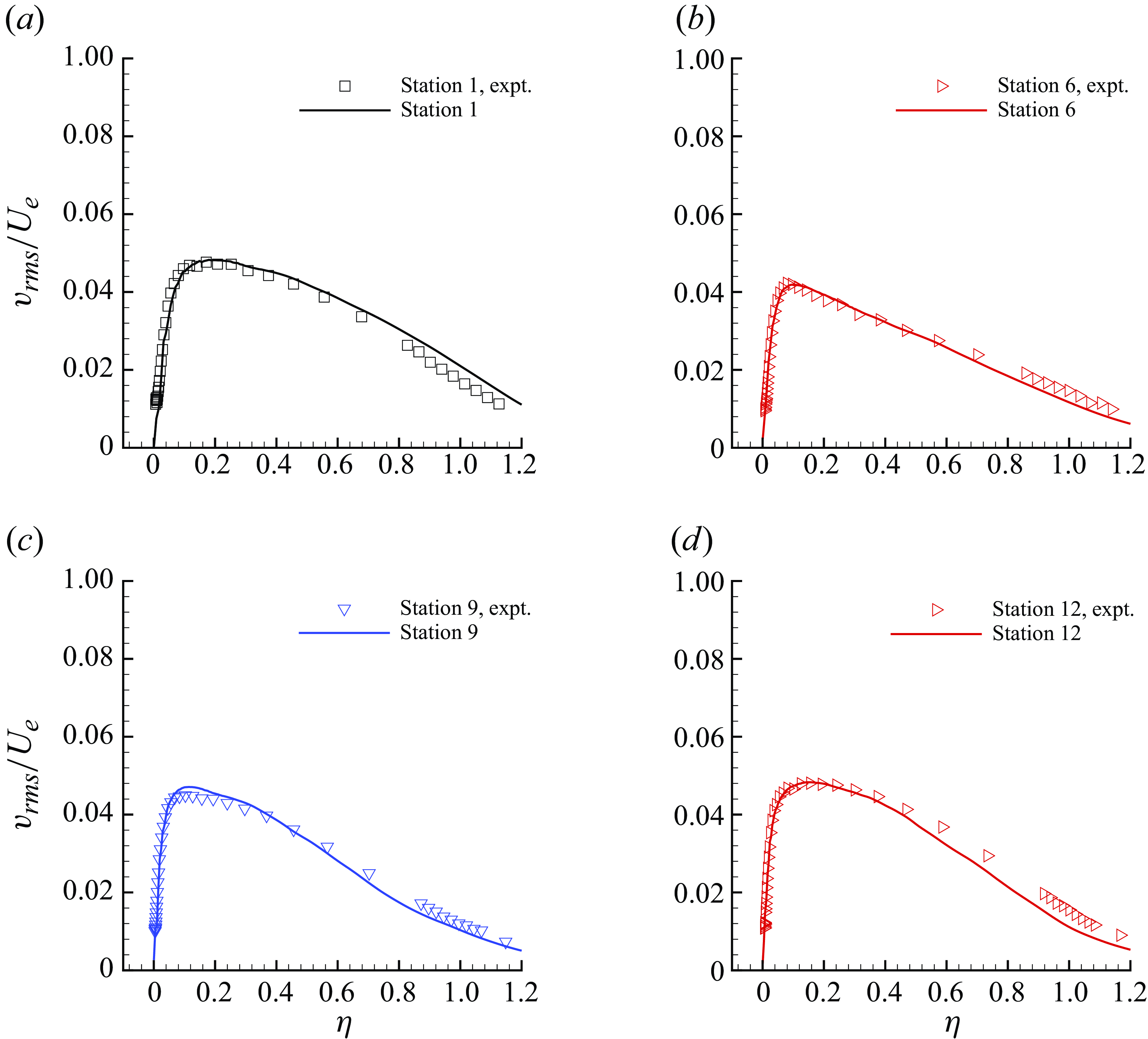
The profiles of mean streamwise velocity, resolved root-mean-square (r.m.s.) fluctuations in streamwise and wall-normal velocities along with Reynolds shear stress are compared with the reference data at selected stations (Stations 1, 6, 9 and 12) in figures 7, 8, 9 and 10, respectively. The profile comparisons at other stations are shown in Appendix C for completeness.
Mean velocity defect profiles (lines) are compared with the reference data (symbols) of Volino (Reference Volino2020a
) at Stations 1, 6 $(a)$
and 9, 12
$(a)$
and 9, 12 $(b)$
.
$(b)$
.
The r.m.s. of streamwise velocity fluctuations (lines) are compared with the reference data (symbols) of Volino (Reference Volino2020a
) at Stations 1 $(a)$
, 6
$(a)$
, 6 $(b)$
, 9
$(b)$
, 9 $(c)$
and 12
$(c)$
and 12 $(d)$
.
$(d)$
.
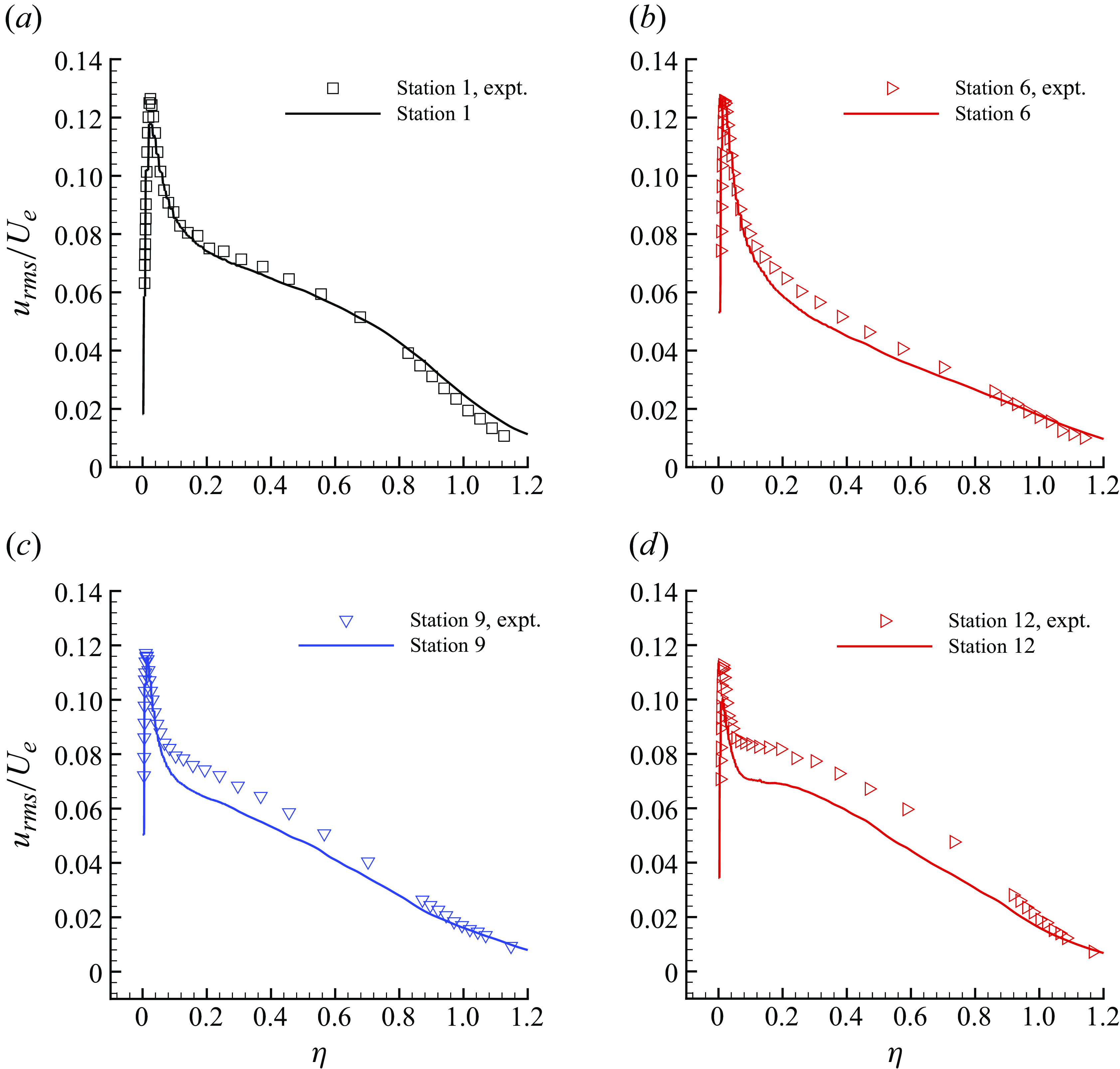
The streamwise velocity profiles are shown in the form of velocity defect normalised by the local free stream velocity. The results show very good agreement at all the stations. The grid is able to capture the defect profile adequately even at Station 6, where the boundary layer thickness is very small. The LES results for the r.m.s. of streamwise velocity show some differences at Stations 6–12 in the outer layer. The profiles of the r.m.s. of wall-normal velocity fluctuations and the Reynolds shear stress show good agreement with the reference data at all the stations.
The r.m.s. of wall-normal velocity fluctuations (lines) are compared with the reference data (symbols) of Volino (Reference Volino2020a
) at Stations 1 $(a)$
, 6
$(a)$
, 6 $(b)$
, 9
$(b)$
, 9 $(c)$
and 12
$(c)$
and 12 $(d)$
.
$(d)$
.
Reynolds shear stress profiles (lines) are compared with the reference data (symbols) of Volino (Reference Volino2020a
) at Stations 1 $(a)$
, 6
$(a)$
, 6 $(b)$
, 9
$(b)$
, 9 $(c)$
and 12
$(c)$
and 12 $(d)$
.
$(d)$
.
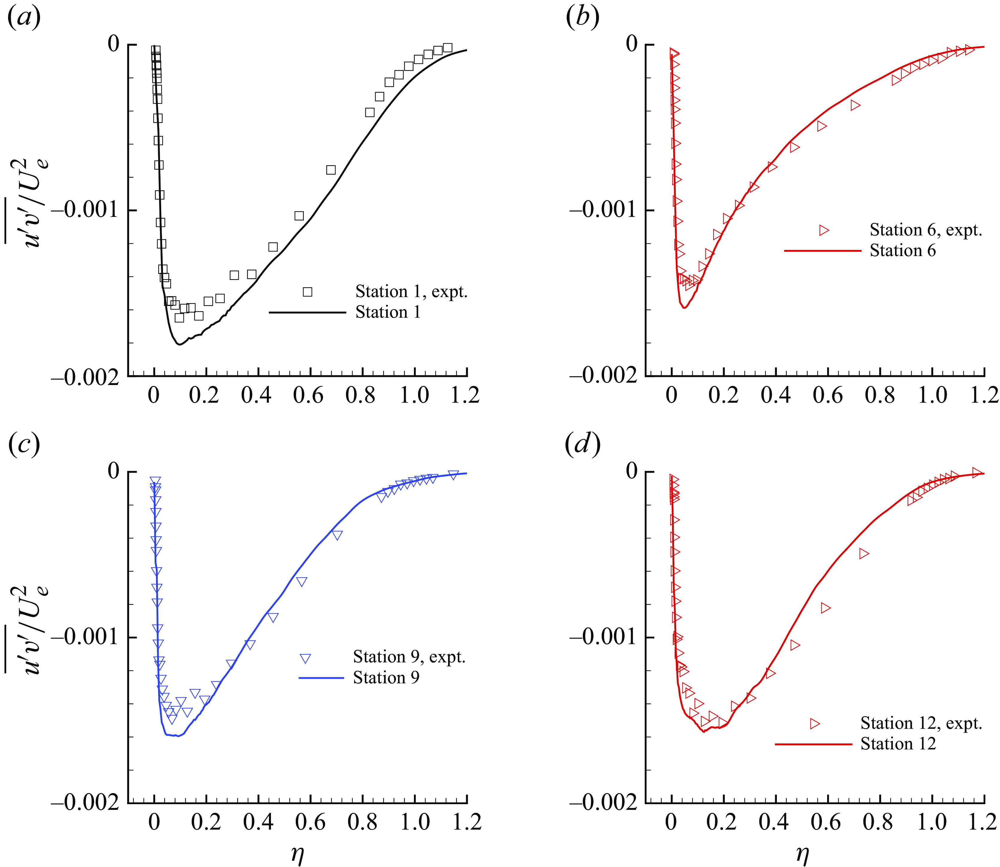
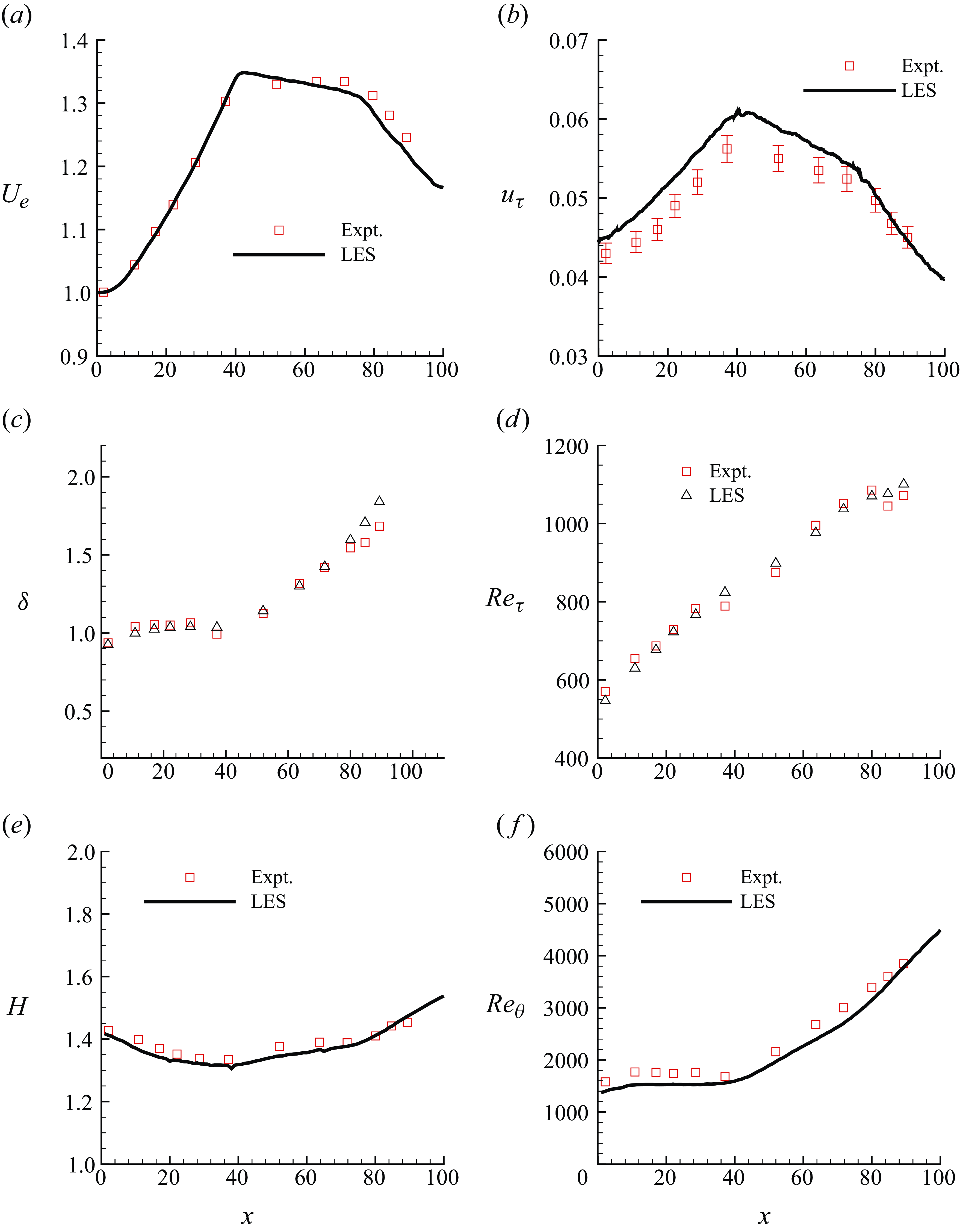
Figure 11 shows the TBL evolution through the flow domain. As observed in figure 11 $(a)$
,
$(a)$
, $(U_e)$
shows good agreement with the reference data in the FPG region. There is a slight mismatch in the recovery and APG regions. In particular, the results show slightly lower
$(U_e)$
shows good agreement with the reference data in the FPG region. There is a slight mismatch in the recovery and APG regions. In particular, the results show slightly lower $U_e$
in the APG region. One possible reason for this behaviour can be the difference in the top wall boundary layer between the LES and the reference experiment. The problem set-up is such that the same mass flow passes through the domain. So if the top wall boundary layer in the present simulation is thinner than the reference experiment,
$U_e$
in the APG region. One possible reason for this behaviour can be the difference in the top wall boundary layer between the LES and the reference experiment. The problem set-up is such that the same mass flow passes through the domain. So if the top wall boundary layer in the present simulation is thinner than the reference experiment, $U_e$
will be smaller at the bottom wall. The LES results indicate that the reference experiment has thicker top wall boundary layer in the APG region than the present simulation. The streamwise evolution of
$U_e$
will be smaller at the bottom wall. The LES results indicate that the reference experiment has thicker top wall boundary layer in the APG region than the present simulation. The streamwise evolution of $u_{\tau }$
on the bottom wall is compared with the reference data in figure 11
$u_{\tau }$
on the bottom wall is compared with the reference data in figure 11 $(b)$
. Volino (Reference Volino2020a
) obtained
$(b)$
. Volino (Reference Volino2020a
) obtained $u_{\tau }$
indirectly from the
$u_{\tau }$
indirectly from the $U$
profile measurements and reported an uncertainty of
$U$
profile measurements and reported an uncertainty of $3 \,\%$
which is shown as error bars. The LES results overpredict
$3 \,\%$
which is shown as error bars. The LES results overpredict $u_{\tau }$
in the FPG and recovery regions. The evolution of
$u_{\tau }$
in the FPG and recovery regions. The evolution of $\delta$
(figure 11
$\delta$
(figure 11 $c$
) is captured well throughout the domain except at the last two stations where there is small mismatch. On the other hand,
$c$
) is captured well throughout the domain except at the last two stations where there is small mismatch. On the other hand, $Re_{\tau }$
(figure 11
$Re_{\tau }$
(figure 11 $d$
) evolution compares well with the reference data throughout the domain. The shape factor (
$d$
) evolution compares well with the reference data throughout the domain. The shape factor ( $H$
) is compared with the reference data in figure 11(
$H$
) is compared with the reference data in figure 11( $e$
), showing good overall agreement. Figure 11(
$e$
), showing good overall agreement. Figure 11( $f$
) shows the evolution of
$f$
) shows the evolution of $Re_{\theta }$
. There is a slight underprediction of
$Re_{\theta }$
. There is a slight underprediction of $Re_{\theta }$
compared with the reference data. This may be reasonable given the comparison of
$Re_{\theta }$
compared with the reference data. This may be reasonable given the comparison of $\delta$
and
$\delta$
and $H$
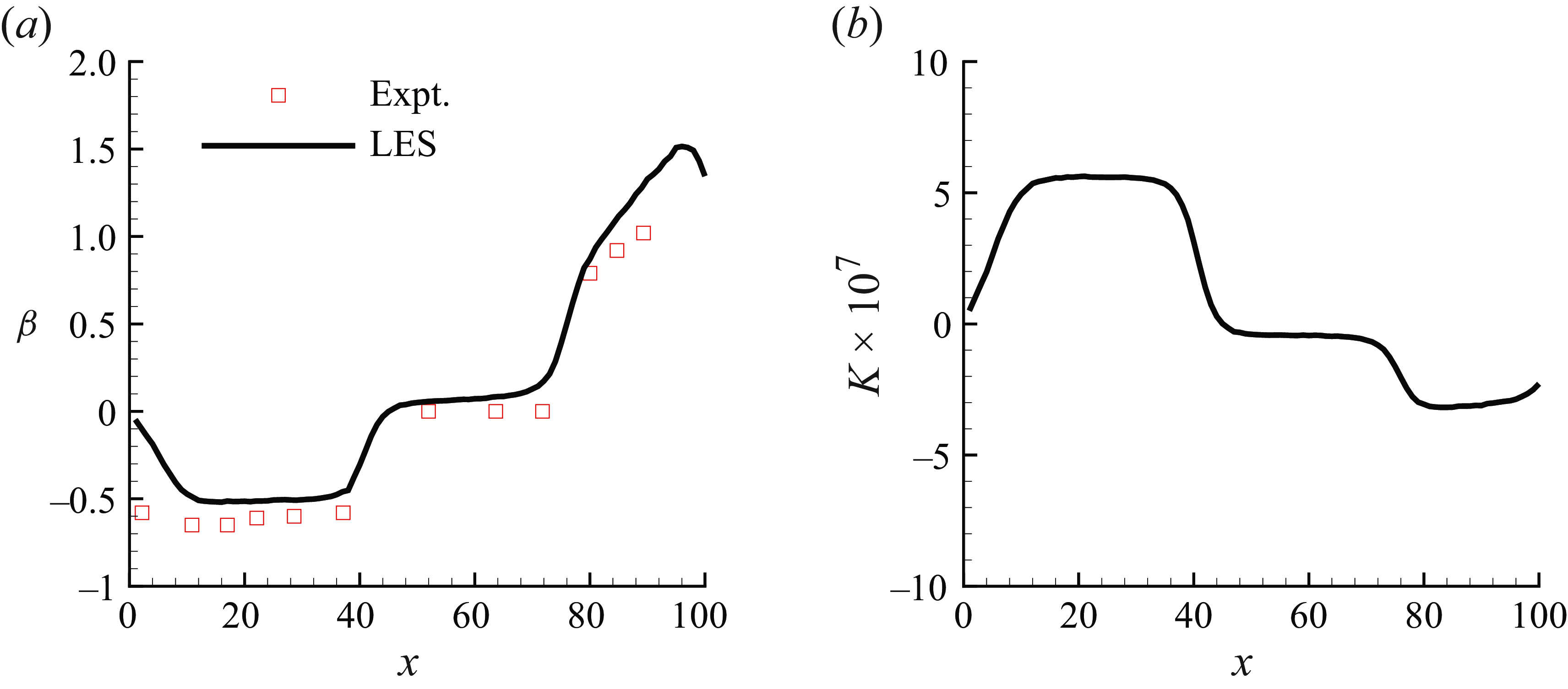
. Figure 12(
$H$
. Figure 12( $a$
) compares
$a$
) compares $(\beta )$
with the reference data. Here
$(\beta )$
with the reference data. Here $\beta \approx 0$
at the inflow, as expected. The magnitude of
$\beta \approx 0$
at the inflow, as expected. The magnitude of $\beta$
is underpredicted at the first few stations. This observation is consistent with the overprediction in
$\beta$
is underpredicted at the first few stations. This observation is consistent with the overprediction in $u_{\tau }$
as shown in figure 11(
$u_{\tau }$
as shown in figure 11( $b$
). Figure 12(
$b$
). Figure 12( $b$
) shows the streamwise variation in
$b$
) shows the streamwise variation in $K$
. Note the value of
$K$
. Note the value of $K$
in the reference experiment was
$K$
in the reference experiment was $5 \times 10^{-7}$
in the FPG region. Here
$5 \times 10^{-7}$
in the FPG region. Here $K$
appears constant in FPG, recovery and APG regions as expected, and its value is close to the reference experiment in the FPG and recovery regions. However,
$K$
appears constant in FPG, recovery and APG regions as expected, and its value is close to the reference experiment in the FPG and recovery regions. However, $K$
is slightly lower in magnitude in the APG region, compared with the experiments where it was set at
$K$
is slightly lower in magnitude in the APG region, compared with the experiments where it was set at $K = - 5 \times 10^{-7}$
. This again can be a consequence of difference in the top wall boundary layer in the present simulation compared with the reference experimental set-up.
$K = - 5 \times 10^{-7}$
. This again can be a consequence of difference in the top wall boundary layer in the present simulation compared with the reference experimental set-up.
Given the complexity of the problem and uncertainty associated with the top-wall boundary layer, the present results for the boundary layer integral quantities can be considered adequate.
Here $U_e$
,
$U_e$
, $(a)$
,
$(a)$
, $u_{\tau }$ $(b)$
,
$(b)$
, $\delta$ $(c)$
,
$(c)$
, $Re_{\tau }$ $(d)$
,
$(d)$
, $H$
$H$ $(e)$
and
$(e)$
and $Re_{\theta }$ $(f)$
are compared with the reference data. Error bars of 3 % are shown in
$(f)$
are compared with the reference data. Error bars of 3 % are shown in $(b)$
as reported in Volino (Reference Volino2020a
). Here
$(b)$
as reported in Volino (Reference Volino2020a
). Here $U_e$
and
$U_e$
and $u_{\tau }$
are normalised with the free stream velocity at the inflow whereas
$u_{\tau }$
are normalised with the free stream velocity at the inflow whereas $\delta$
is normalised with the inflow boundary layer thickness.
$\delta$
is normalised with the inflow boundary layer thickness.
The streamwise variation in $\beta$ $(a)$
and
$(a)$
and $K$
$K$ $(b)$
.
$(b)$
.
4. Analysis
4.1. Scaling behaviour
Appropriate length and velocity scales in TBL have been widely studied in the literature. In particular, $U_e$
and
$U_e$
and $\delta$
are often used as appropriate scales to collapse defect profiles in the outer layer of TBL. Volino (Reference Volino2020a
) showed that defect profiles did not collapse using
$\delta$
are often used as appropriate scales to collapse defect profiles in the outer layer of TBL. Volino (Reference Volino2020a
) showed that defect profiles did not collapse using $U_e$
and
$U_e$
and $\delta$
. In the present section, appropriate length and velocity scales are sought for the present case using the reference data of Volino (Reference Volino2020a
).
$\delta$
. In the present section, appropriate length and velocity scales are sought for the present case using the reference data of Volino (Reference Volino2020a
).
Zagarola & Smits (Reference Zagarola and Smits1998a
) proposed a velocity scale ( $u_{zs} = U_e \delta ^*/\delta$
, called the ZS scaling henceforth) for pipe flow as an appropriate outer velocity scale, which was able to collapse the outer-layer velocity profiles. The ZS velocity scale was later found to be appropriate even for ZPG TBL (Zagarola & Smits Reference Zagarola and Smits1998b
; George Reference George2006). Wei & Maciel (Reference Wei and Maciel2018) derived
$u_{zs} = U_e \delta ^*/\delta$
, called the ZS scaling henceforth) for pipe flow as an appropriate outer velocity scale, which was able to collapse the outer-layer velocity profiles. The ZS velocity scale was later found to be appropriate even for ZPG TBL (Zagarola & Smits Reference Zagarola and Smits1998b
; George Reference George2006). Wei & Maciel (Reference Wei and Maciel2018) derived $u_{zs}$
from the mean continuity equation in ZPG TBL. Maciel et al. (Reference Maciel, Wei, Gungor and Simens2018) analysed the scaling of APG TBL and concluded that
$u_{zs}$
from the mean continuity equation in ZPG TBL. Maciel et al. (Reference Maciel, Wei, Gungor and Simens2018) analysed the scaling of APG TBL and concluded that $u_{zs}$
was appropriate velocity scale for a variety of TBL databases they analysed.
$u_{zs}$
was appropriate velocity scale for a variety of TBL databases they analysed.
Recently, Pirozzoli & Smits (Reference Pirozzoli and Smits2023) proposed a new set of velocity ( $u_{ps}$
) and length (
$u_{ps}$
) and length ( $\delta _{ps}$
) scales for outer layer of TBL (called the PS scaling henceforth) given by
$\delta _{ps}$
) scales for outer layer of TBL (called the PS scaling henceforth) given by
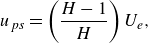 \begin{eqnarray} u_{ps} = \left (\frac {H-1}{H} \right ) U_e, \end{eqnarray}
 \begin{eqnarray} \delta _{ps} = \left (\frac {H}{H -1} \right ) \delta ^*. \end{eqnarray}
They tested their scaling on various ZPG TBL databases showing good collapse in the outer layer. It remains unclear if ZS and PS scalings would hold for a non-equilibrium TBL such as the present case.
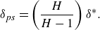
The applicability of ZS and PS scales is assessed in figure 13 using the reference experimental data. The results show that both these scalings collapse the velocity defect profiles adequately well in the outer layer, with PS scaling performing slightly better as one moves closer to the wall. The PS scaling is able to collapse the defect profiles in the FPG, ZPG and APG regions adequately, suggesting that even the non-equilibrium effects are adequately captured in $u_{ps}$
and
$u_{ps}$
and $\delta _{ps}$
. Overall, it can be concluded that PS scaling appears to be generally applicable to TBL ranging for equilibrium, near-equilibrium and the present non-equilibrium case. However, its applicability to stronger non-equilibrium cases is yet to be evaluated.
$\delta _{ps}$
. Overall, it can be concluded that PS scaling appears to be generally applicable to TBL ranging for equilibrium, near-equilibrium and the present non-equilibrium case. However, its applicability to stronger non-equilibrium cases is yet to be evaluated.
Velocity defect in the scaling proposed by Zagarola & Smits (Reference Zagarola and Smits1998a
) ( $a$
) and Pirozzoli & Smits (Reference Pirozzoli and Smits2023) (
$a$
) and Pirozzoli & Smits (Reference Pirozzoli and Smits2023) ( $b$
) at all the stations.
$b$
) at all the stations.
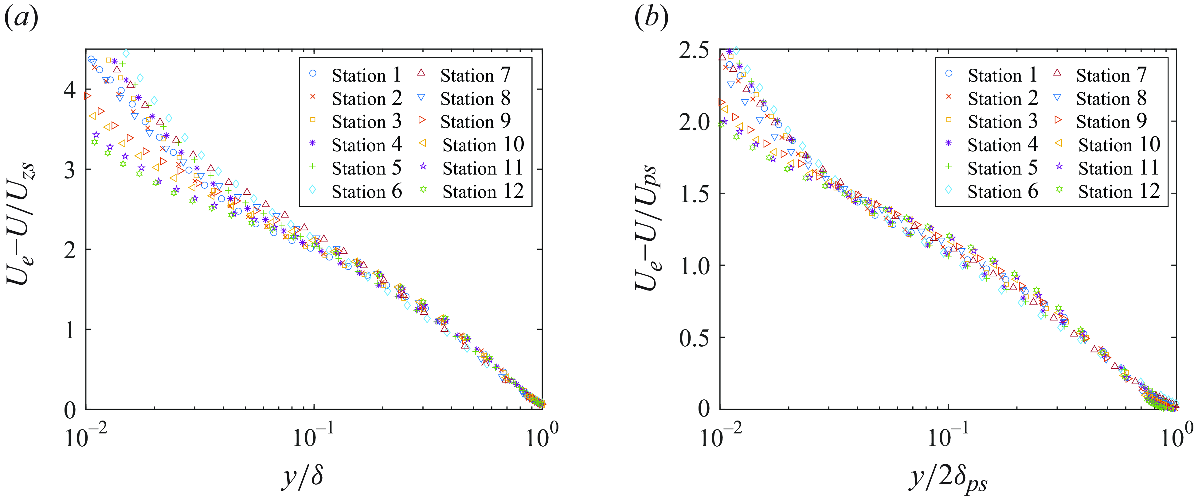
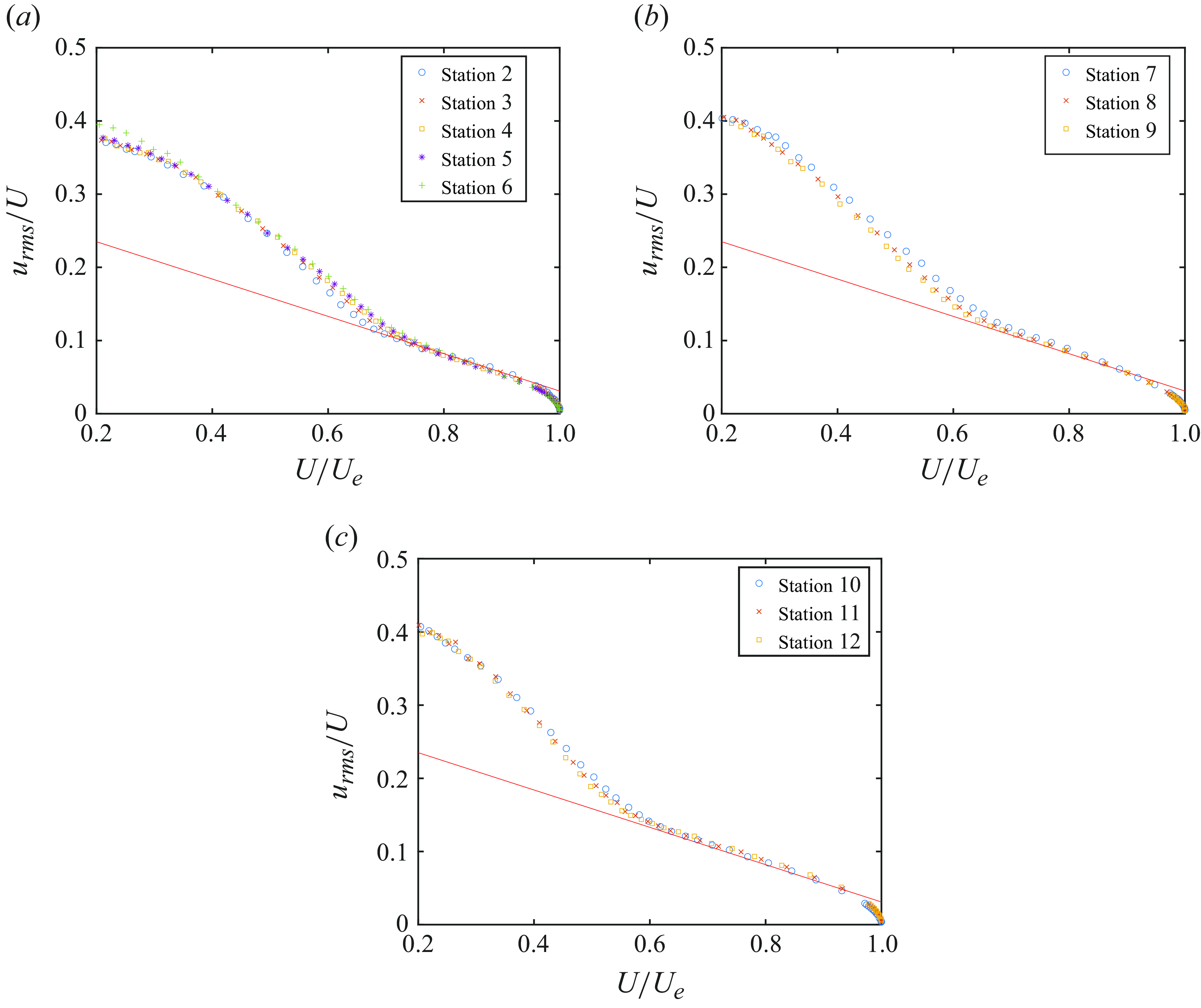
Next, the scaling of $u_{rms}$
is considered. Alfredsson, Segalini & Örlü (Reference Alfredsson, Segalini and Örlü2011) proposed a scaling for
$u_{rms}$
is considered. Alfredsson, Segalini & Örlü (Reference Alfredsson, Segalini and Örlü2011) proposed a scaling for $u_{rms}$
in the outer layer in the TBL,
$u_{rms}$
in the outer layer in the TBL,
 \begin{eqnarray} \frac {u_{rms}}{U} = a + b \frac {U}{U_e}, \end{eqnarray}
where $a = 0.286$
and
$a = 0.286$
and $b = -0.255$
, which was also found to hold for other wall-bounded flows (Alfredsson, Örlü & Segalini Reference Alfredsson, Örlü and Segalini2012). Figure 14 shows
$b = -0.255$
, which was also found to hold for other wall-bounded flows (Alfredsson, Örlü & Segalini Reference Alfredsson, Örlü and Segalini2012). Figure 14 shows $u_{rms}/U$
profiles plotted against
$u_{rms}/U$
profiles plotted against $U/U_e$
for the FPG, ZPG and APG regions. The line in the figures correspond to (4.3) evaluated at Station 2, Station 7 and Station 10 in figures 14
$U/U_e$
for the FPG, ZPG and APG regions. The line in the figures correspond to (4.3) evaluated at Station 2, Station 7 and Station 10 in figures 14 $(a)$
, 14
$(a)$
, 14 $(b)$
and 14
$(b)$
and 14 $(c)$
, respectively. The profiles collapse to (4.3) surprisingly well in all three regions. Note that Stations 2, 7 and 10 are chosen as they are the first station in each of these regions. Choosing a different station to evaluate (4.3) would not make any difference in the results. It is worth mentioning that Dróżdż et al. (Reference Dróżdż, Elsner and Drobniak2015) proposed a modification to (4.3) for pressure gradient TBL by including
$(c)$
, respectively. The profiles collapse to (4.3) surprisingly well in all three regions. Note that Stations 2, 7 and 10 are chosen as they are the first station in each of these regions. Choosing a different station to evaluate (4.3) would not make any difference in the results. It is worth mentioning that Dróżdż et al. (Reference Dróżdż, Elsner and Drobniak2015) proposed a modification to (4.3) for pressure gradient TBL by including $\sqrt {H}$
in the denominator of the left-hand side and modifying the values of
$\sqrt {H}$
in the denominator of the left-hand side and modifying the values of $a$
and
$a$
and $b$
for different pressure gradient conditions. It appears that such modifications are not needed for the present case where (4.3) adequately describes the linear region in figure 14.
$b$
for different pressure gradient conditions. It appears that such modifications are not needed for the present case where (4.3) adequately describes the linear region in figure 14.
Here $u_{rms}/U$
profiles in FPG (
$u_{rms}/U$
profiles in FPG ( $a$
), ZPG (
$a$
), ZPG ( $b$
) and APG (
$b$
) and APG ( $c$
) regions along with (4.3) (line) evaluated at Station 2 in
$c$
) regions along with (4.3) (line) evaluated at Station 2 in $(a)$
, Station 7 in
$(a)$
, Station 7 in $(b)$
and Station 10 in
$(b)$
and Station 10 in $(c)$
.
$(c)$
.
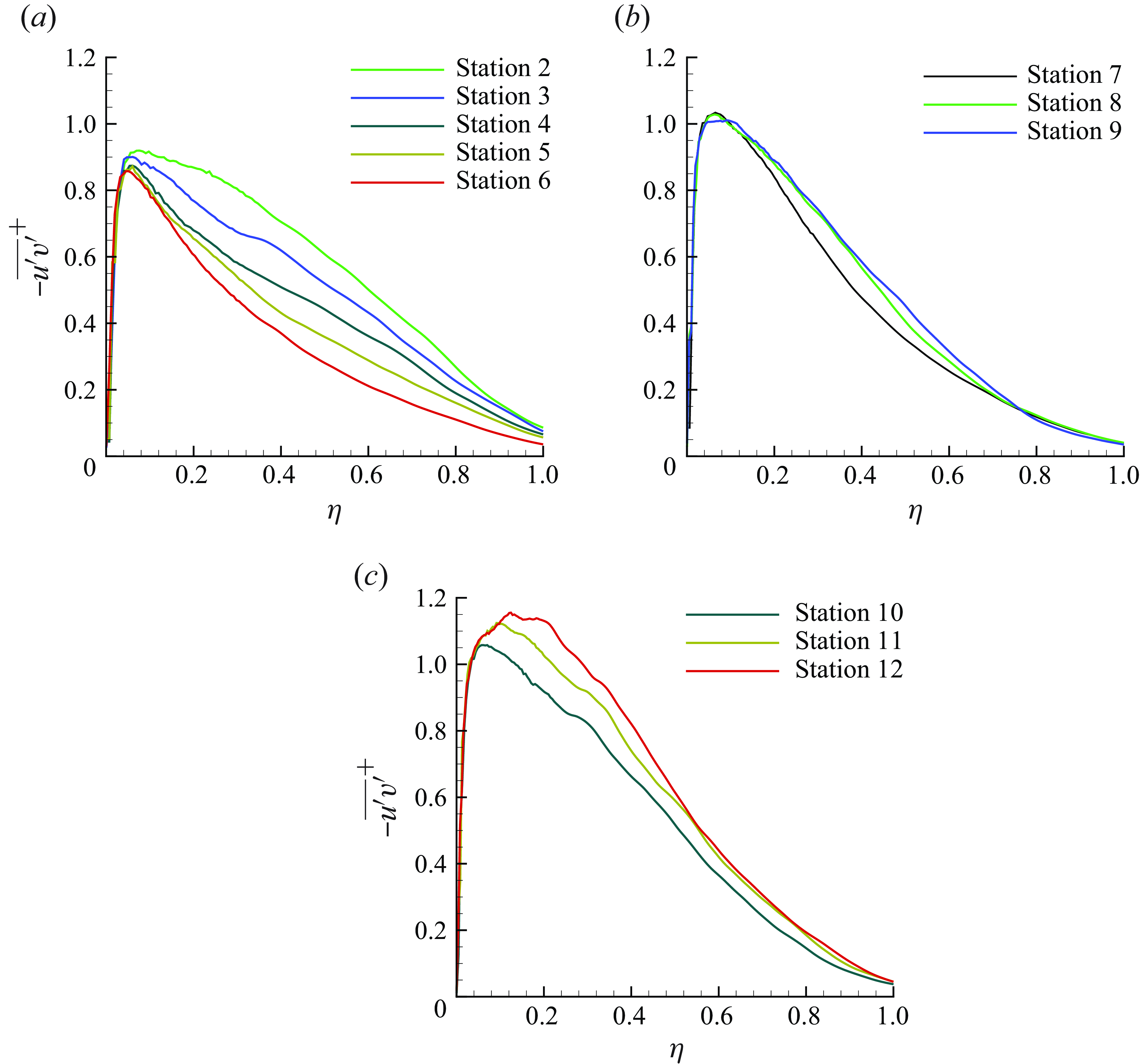
4.2. Modelling implications
Mean total shear stress $(T)$
in the TBL is the sum of viscous and Reynolds shear stress. In the outer layer, the viscous stress is negligible. Hence,
$(T)$
in the TBL is the sum of viscous and Reynolds shear stress. In the outer layer, the viscous stress is negligible. Hence, $T \approx -\overline {u'v'}$
in the outer layer. Kumar & Mahesh (Reference Kumar and Mahesh2021) observed that
$T \approx -\overline {u'v'}$
in the outer layer. Kumar & Mahesh (Reference Kumar and Mahesh2021) observed that $T^+$
plotted against
$T^+$
plotted against $\eta$
was insensitive to
$\eta$
was insensitive to $Re$
for ZPG TBLs. This observation holds even for APG TBL under near-equilibrium conditions when
$Re$
for ZPG TBLs. This observation holds even for APG TBL under near-equilibrium conditions when $\beta$
is held constant (Kumar & Mahesh Reference Kumar and Mahesh2022). Figure 15 shows
$\beta$
is held constant (Kumar & Mahesh Reference Kumar and Mahesh2022). Figure 15 shows $-\overline {u'v'}^+$
plotted against
$-\overline {u'v'}^+$
plotted against $\eta$
in the FPG, recovery and APG regions. It is observed that the mean shear stress in the outer layer does not collapse onto a single curve, except in the recovery region where the pressure gradient is negligible and a reasonable collapse is observed for Stations 8 and 9. In the FPG region,
$\eta$
in the FPG, recovery and APG regions. It is observed that the mean shear stress in the outer layer does not collapse onto a single curve, except in the recovery region where the pressure gradient is negligible and a reasonable collapse is observed for Stations 8 and 9. In the FPG region, $-\overline {u'v'}^+$
kepng decreasing from Station 2–6 for a given
$-\overline {u'v'}^+$
kepng decreasing from Station 2–6 for a given $\eta$
for
$\eta$
for $\eta \gt 0.1$
. The trend is opposite in the APG region. Therefore, the total shear stress model of Kumar & Mahesh (Reference Kumar and Mahesh2022) derived for near-equilibrium pressure-gradient TBL (i.e.
$\eta \gt 0.1$
. The trend is opposite in the APG region. Therefore, the total shear stress model of Kumar & Mahesh (Reference Kumar and Mahesh2022) derived for near-equilibrium pressure-gradient TBL (i.e. $\beta$
held constant) is not expected to work for the present case.
$\beta$
held constant) is not expected to work for the present case.
Reynolds shear stress profiles in FPG $(a)$
, recovery
$(a)$
, recovery $(b)$
and APG
$(b)$
and APG $(c)$
regions.
$(c)$
regions.
Kumar & Mahesh (Reference Kumar and Mahesh2021) also proposed a model for wall-normal velocity $(V)$
in ZPG TBL. They observed that
$(V)$
in ZPG TBL. They observed that $V$
scaled with its edge value collapse well for a range of
$V$
scaled with its edge value collapse well for a range of $Re$
when plotted against
$Re$
when plotted against $\eta$
. This led them to fit a hyperbolic tangent function with two constants to obtain a model for
$\eta$
. This led them to fit a hyperbolic tangent function with two constants to obtain a model for $V$
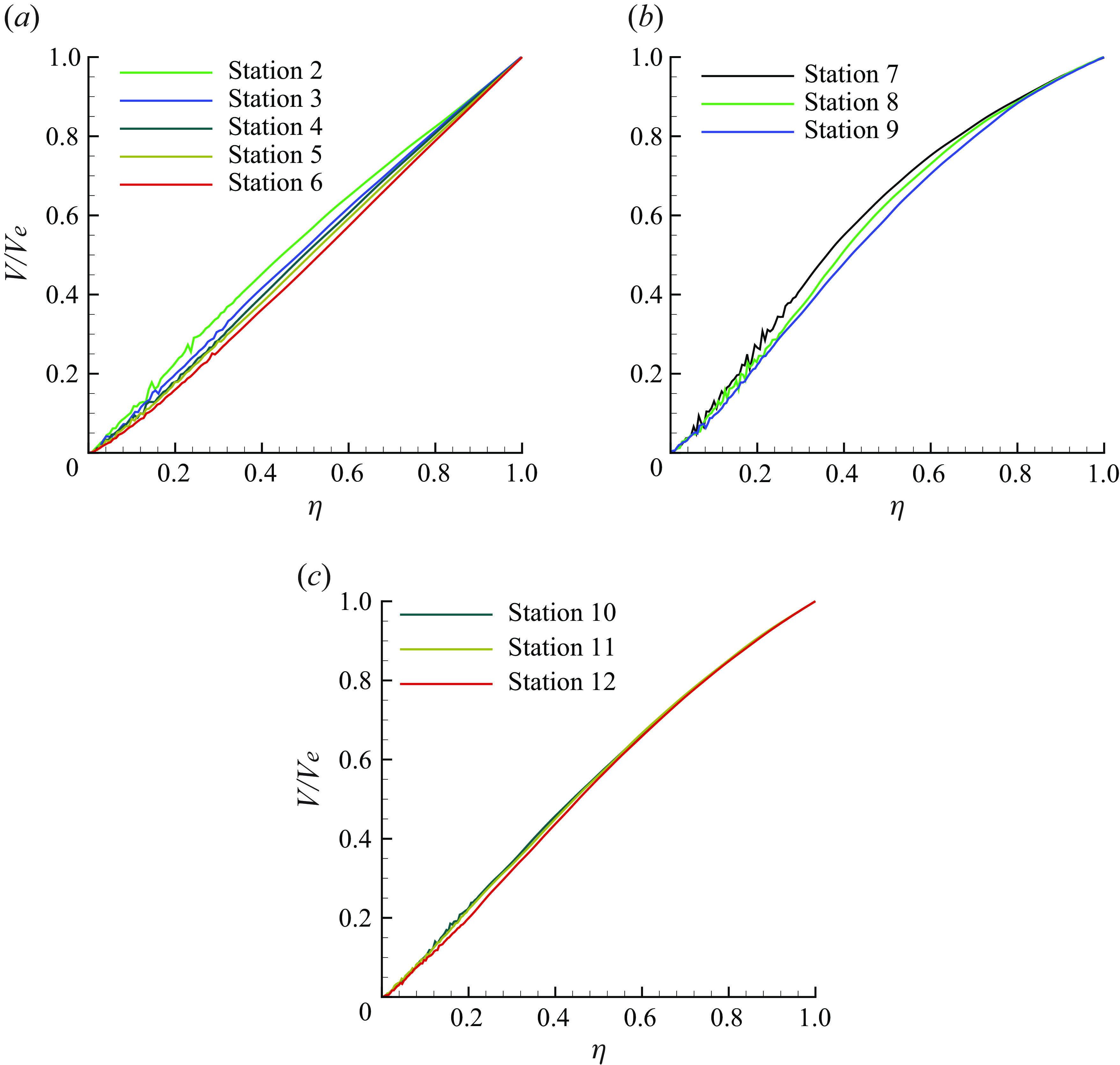
. Later, they extended the model for pressure-gradient TBL by simply multiplying it by a function to enforce it to satisfy the continuity equation outside the boundary layer. Figure 16 shows
$V$
. Later, they extended the model for pressure-gradient TBL by simply multiplying it by a function to enforce it to satisfy the continuity equation outside the boundary layer. Figure 16 shows $V/V_e$
plotted as a function of
$V/V_e$
plotted as a function of $\eta$
for the FPG, recovery and APG regions. First thing to note is that
$\eta$
for the FPG, recovery and APG regions. First thing to note is that $V_e$
appears to be appropriate scale for
$V_e$
appears to be appropriate scale for $V$
even in non-equilibrium TBL. The collapse is the best in the APG region. It is interesting to observe that the shape of
$V$
even in non-equilibrium TBL. The collapse is the best in the APG region. It is interesting to observe that the shape of $V/V_e$
is very different than what is observed for equilibrium and near-equilibrium TBL (Kumar & Mahesh Reference Kumar and Mahesh2021, Reference Kumar and Mahesh2022). Even in the recovery region, which is nominally at ZPG conditions, the profile shape of
$V/V_e$
is very different than what is observed for equilibrium and near-equilibrium TBL (Kumar & Mahesh Reference Kumar and Mahesh2021, Reference Kumar and Mahesh2022). Even in the recovery region, which is nominally at ZPG conditions, the profile shape of $V/V_e$
deviates significantly from the ZPG TBL profiles shown in Kumar & Mahesh (Reference Kumar and Mahesh2021). This behaviour suggests that the
$V/V_e$
deviates significantly from the ZPG TBL profiles shown in Kumar & Mahesh (Reference Kumar and Mahesh2021). This behaviour suggests that the $V/V_e$
model of Kumar & Mahesh (Reference Kumar and Mahesh2022) which showed good performance for near-equilibrium TBL may not hold in non-equilibrium TBL.
$V/V_e$
model of Kumar & Mahesh (Reference Kumar and Mahesh2022) which showed good performance for near-equilibrium TBL may not hold in non-equilibrium TBL.
In particular, it appears that $V/V_e \approx \eta$
in FPG and APG regions. This behaviour can be explained using continuity equation as follows. Using the continuity equation for mean flow, it can be shown that
$V/V_e \approx \eta$
in FPG and APG regions. This behaviour can be explained using continuity equation as follows. Using the continuity equation for mean flow, it can be shown that
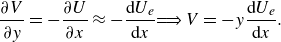 \begin{eqnarray} \frac {\partial V}{\partial y} = - \frac {\partial U}{\partial x} \approx - \frac {{\textrm d} U_e}{{\textrm d} x} \implies V = - y \frac {{\textrm d} U_e}{{\textrm d} x}. \end{eqnarray}
It is easy to see that (4.4) will lead to $V/V_e \approx \eta$
, as observed in FPG (figure 16
$V/V_e \approx \eta$
, as observed in FPG (figure 16 $a$
) and APG (figure 16
$a$
) and APG (figure 16 $c$
) regions.
$c$
) regions.
Mean wall-normal velocity profiles in FPG $(a)$
, recovery
$(a)$
, recovery $(b)$
and APG
$(b)$
and APG $(c)$
regions.
$(c)$
regions.
4.3. Response of TBL to non-equilibrium conditions
In the present study, an equilibrium TBL evolves under streamwise varying pressure gradient conditions, from favourable to zero to adverse. In order to understand the response of the TBL to such non-equilibrium conditions, Volino (Reference Volino2020a
) plotted the difference in velocity defect ( $A_{ZPG} - A$
) as a function of streamwise location at
$A_{ZPG} - A$
) as a function of streamwise location at $\eta = 0.4$
, where
$\eta = 0.4$
, where $A = (U_e - U)/U_e$
. Here
$A = (U_e - U)/U_e$
. Here $A_{ZPG}$
was obtained from the prior ZPG experiments (Volino Reference Volino2020b
). Here, a change function
$A_{ZPG}$
was obtained from the prior ZPG experiments (Volino Reference Volino2020b
). Here, a change function $\varDelta (f) = f - f_{0}$
is defined, where
$\varDelta (f) = f - f_{0}$
is defined, where $f$
is a flow quantity and the subscript ‘0’ denotes the inflow plane. Here
$f$
is a flow quantity and the subscript ‘0’ denotes the inflow plane. Here $\varDelta$
quantifies the change in a flow quantity with respect to the inflow plane as the TBL evolves through the domain.
$\varDelta$
quantifies the change in a flow quantity with respect to the inflow plane as the TBL evolves through the domain.
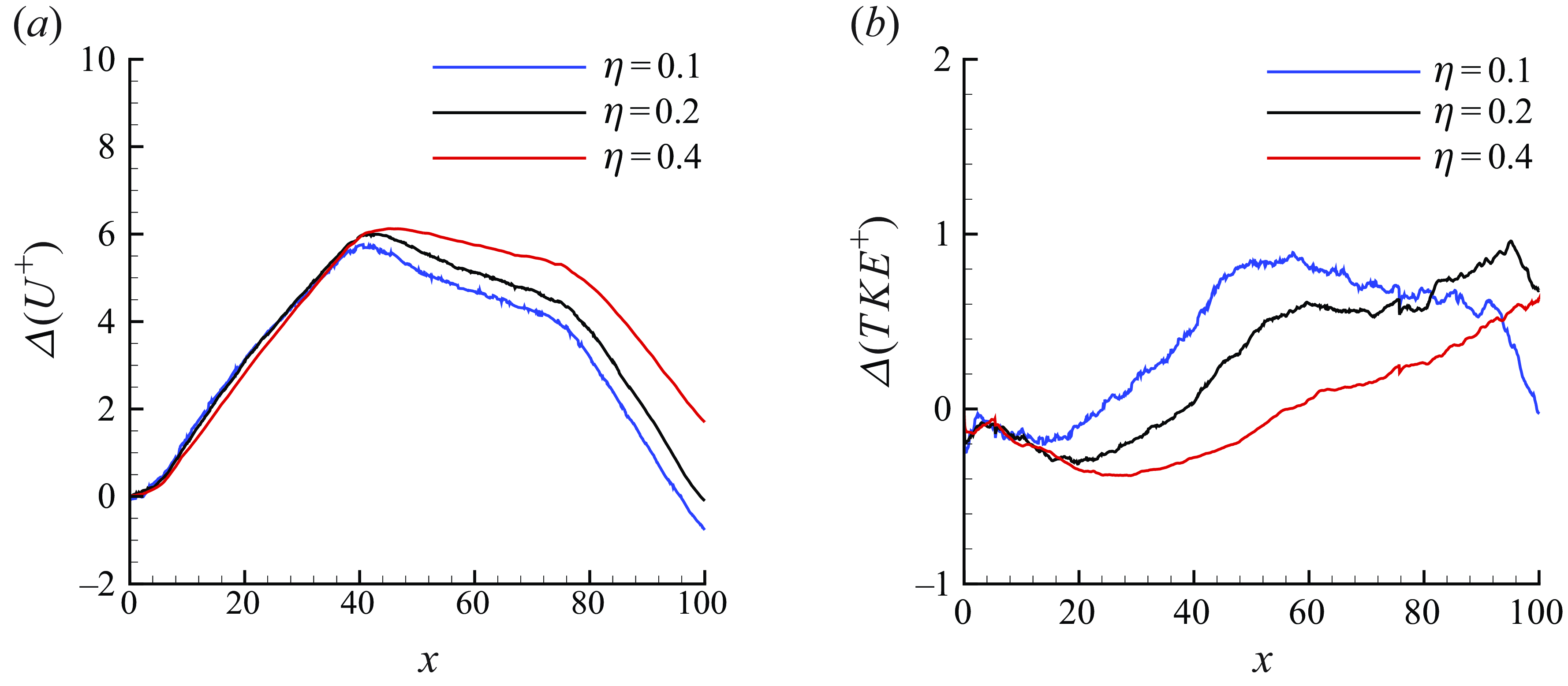
Streamwise evolution of the change in $U^+$
$U^+$ $(a)$
and
$(a)$
and $TKE^+$ $(b)$
at
$(b)$
at $\eta = 0.1$
, 0.2 and 0.4.
$\eta = 0.1$
, 0.2 and 0.4.
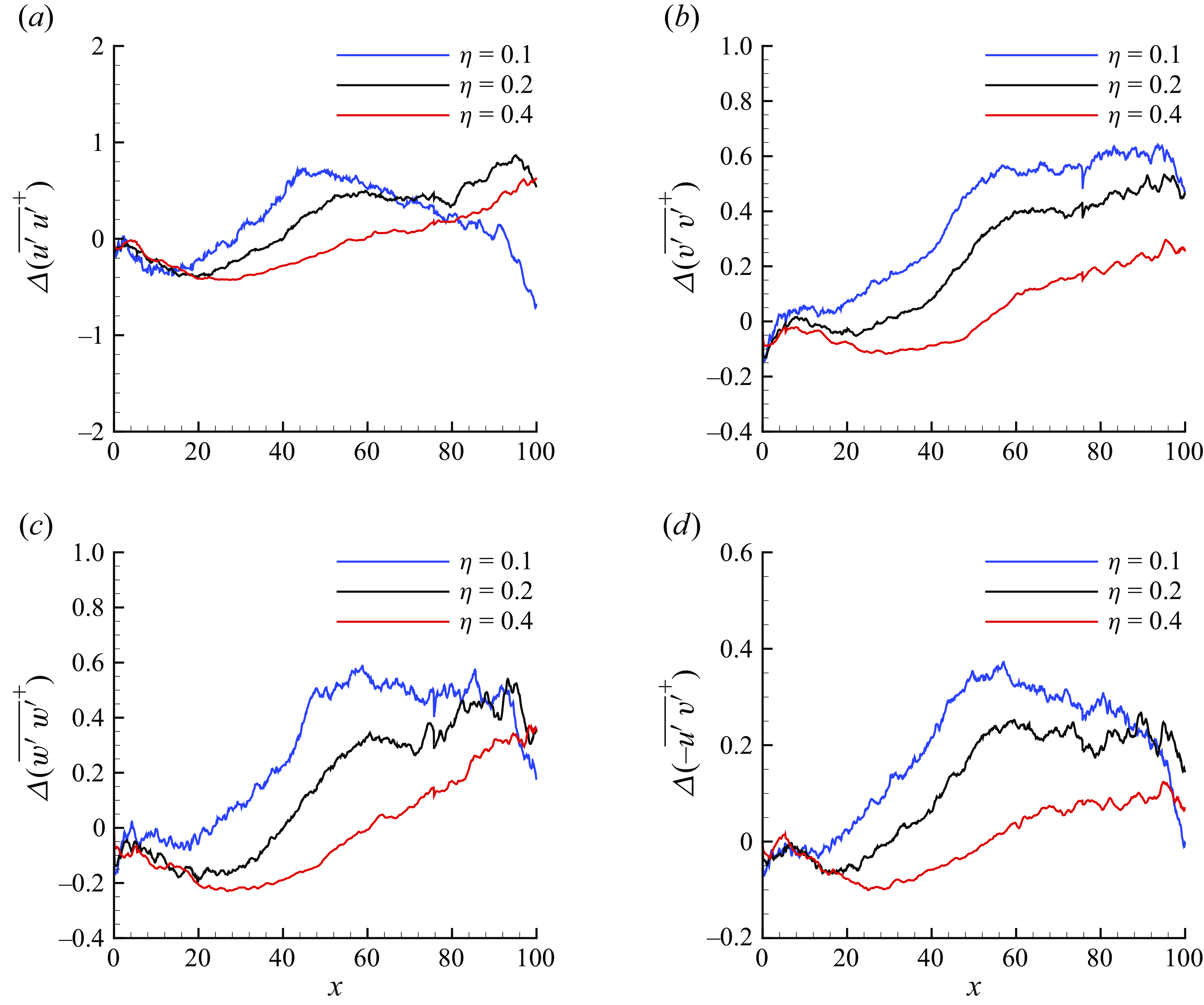
Streamwise evolution of the change in Reynolds stress components: $\overline {u'u'}^+$ $(a)$
;
$(a)$
; $\overline {v'v'}^+$ $(b)$
;
$(b)$
; $\overline {w'w'}^+$ $(c)$
;
$(c)$
; $-\overline {u'v'}^+$ $(d)$
at
$(d)$
at $\eta = 0.1$
, 0.2 and 0.4.
$\eta = 0.1$
, 0.2 and 0.4.
The $\varDelta$
of
$\varDelta$
of $U$
and turbulent kinetic energy (
$U$
and turbulent kinetic energy ( $TKE$
) in inner units are shown in figure 17 at three constants
$TKE$
) in inner units are shown in figure 17 at three constants $\eta = 0.1$
, 0.2 and 0.4. Note that for a ZPG TBL,
$\eta = 0.1$
, 0.2 and 0.4. Note that for a ZPG TBL, $\eta \lt 0.2$
is approximately the extent of the inner layer. Therefore,
$\eta \lt 0.2$
is approximately the extent of the inner layer. Therefore, $\eta = 0.1$
and
$\eta = 0.1$
and $\eta =0.4$
location in TBL can be considered to represent the inner and outer layer, respectively. Recall that the FPG region extends from
$\eta =0.4$
location in TBL can be considered to represent the inner and outer layer, respectively. Recall that the FPG region extends from $x=5.46$
to 40.64, followed by a recovery region up to
$x=5.46$
to 40.64, followed by a recovery region up to $x=75.75$
and an APG region until
$x=75.75$
and an APG region until $x=102.61$
.
$x=102.61$
.
The $\varDelta (U^+)$
at the shown
$\varDelta (U^+)$
at the shown $\eta$
locations appears identical in the FPG region, beyond which the change increases as
$\eta$
locations appears identical in the FPG region, beyond which the change increases as $\eta$
increases throughout the rest of the flow domain. The plot suggests that the response of the inner scaled velocity field to the FPG condition is same at all shown
$\eta$
increases throughout the rest of the flow domain. The plot suggests that the response of the inner scaled velocity field to the FPG condition is same at all shown $\eta$
locations. In the subsequent regions,
$\eta$
locations. In the subsequent regions, $\varDelta (U^+)$
increases with increase in
$\varDelta (U^+)$
increases with increase in $\eta$
. The response of
$\eta$
. The response of $TKE$
(figure 17
$TKE$
(figure 17 $b$
) appears similar at all
$b$
) appears similar at all $\eta$
locations until halfway in the FPG region, beyond which the lowest
$\eta$
locations until halfway in the FPG region, beyond which the lowest $\eta$
location shows the largest value until the end of the recovery region. In the APG region, the
$\eta$
location shows the largest value until the end of the recovery region. In the APG region, the $\varDelta$
in
$\varDelta$
in $TKE$
decreases for
$TKE$
decreases for $\eta =0.1$
, whereas the other
$\eta =0.1$
, whereas the other $\eta$
locations show an increase.
$\eta$
locations show an increase.
In order to better understand the response of TBL, the change in different components of the Reynolds stress tensor are shown in figure 18 at the same $\eta$
locations as figure 17. The
$\eta$
locations as figure 17. The $\varDelta$
in the streamwise component shows identical decrease in the first-half of the FPG region at all
$\varDelta$
in the streamwise component shows identical decrease in the first-half of the FPG region at all $\eta$
locations, beyond which all the
$\eta$
locations, beyond which all the $\eta$
locations show increasing trend for rest of the FPG region. In the APG region, the
$\eta$
locations show increasing trend for rest of the FPG region. In the APG region, the $\eta =0.1$
location shows a decrease, whereas the other locations maintain an increasing trend. This is consistent with the APG TBL behaviour where the streamwise component increases in the outer layer as the TBL evolves. The
$\eta =0.1$
location shows a decrease, whereas the other locations maintain an increasing trend. This is consistent with the APG TBL behaviour where the streamwise component increases in the outer layer as the TBL evolves. The $\varDelta$
in the wall-normal component shows increasing trend throughout the domain, whereas the spanwise component behaves similar to the streamwise component. So the behaviour of
$\varDelta$
in the wall-normal component shows increasing trend throughout the domain, whereas the spanwise component behaves similar to the streamwise component. So the behaviour of $TKE$
where it drops in the latter-half of the APG region at
$TKE$
where it drops in the latter-half of the APG region at $\eta =0.1$
appears to be the result of drop in streamwise component. The Reynolds shear stress increases from the middle of the FPG until the middle of the recovery region, followed by a nearly constant value until the mid of the APG region, and subsequent drop in the rest of the APG region.
$\eta =0.1$
appears to be the result of drop in streamwise component. The Reynolds shear stress increases from the middle of the FPG until the middle of the recovery region, followed by a nearly constant value until the mid of the APG region, and subsequent drop in the rest of the APG region.
The Reynolds stress components can be used to define anisotropy tensor as
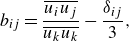 \begin{equation} b_{ij} = \displaystyle\frac {\overline {u_iu_j}}{\overline {u_ku_k}} - \displaystyle\frac {\delta _{ij}}{3}, \end{equation}
where $\delta _{ij}$
is the Kronecker delta. In the limit of one-dimensional turbulence,
$\delta _{ij}$
is the Kronecker delta. In the limit of one-dimensional turbulence, $b_{11} = 2/3$
and
$b_{11} = 2/3$
and
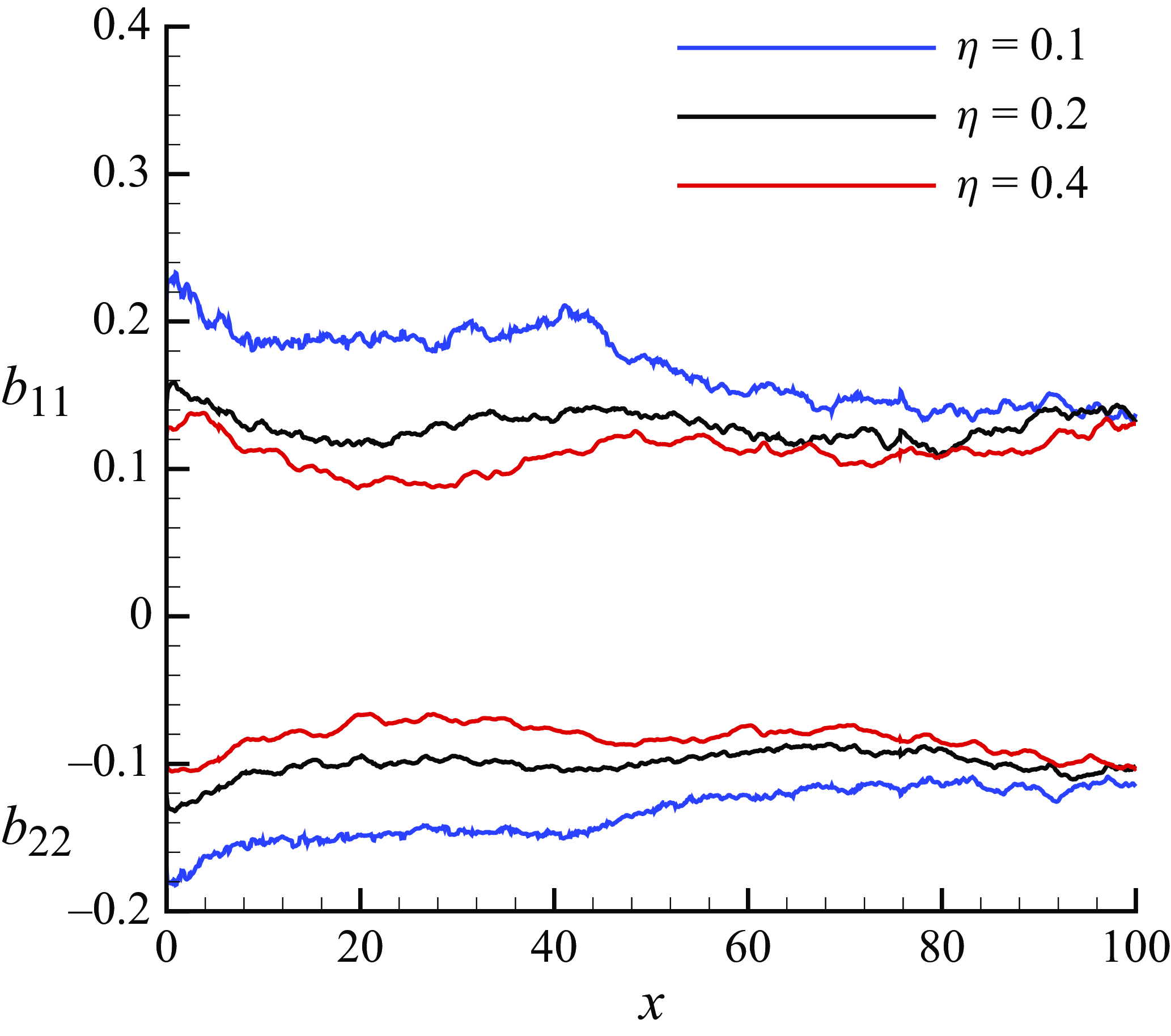
 $b_{22} = b_{33} = -1/3$
. Figure 19 shows the streamwise variation in
$b_{22} = b_{33} = -1/3$
. Figure 19 shows the streamwise variation in $b_{11}$
and
$b_{11}$
and $b_{22}$
at three constant
$b_{22}$
at three constant $\eta$
locations. As expected,
$\eta$
locations. As expected, $b_{11}$
and
$b_{11}$
and $b_{22}$
are quite different than the one-dimensional limiting values. The values remain fairly constant beyond the middle of the FPG region for
$b_{22}$
are quite different than the one-dimensional limiting values. The values remain fairly constant beyond the middle of the FPG region for $\eta =0.2$
and 0.4 locations, suggesting that the anisotropy of the flow does not change in the latter-half of the domain at these locations. The
$\eta =0.2$
and 0.4 locations, suggesting that the anisotropy of the flow does not change in the latter-half of the domain at these locations. The $\eta =0.1$
location shows the largest variation, where
$\eta =0.1$
location shows the largest variation, where $b_{11}$
decreases while
$b_{11}$
decreases while $b_{22}$
increases starting from the recovery region.
$b_{22}$
increases starting from the recovery region.
Streamwise evolution of $b_{11}$ $(a)$
and
$(a)$
and $b_{22}$ $(b)$
at
$(b)$
at $\eta = 0.1$
, 0.2 and 0.4.
$\eta = 0.1$
, 0.2 and 0.4.
5. Summary
Wall-resolved LES of a non-equilibrium smooth wall TBL is performed, closely matching the experimental set-up of Volino (Reference Volino2020a ). The computational domain is carefully chosen to match the physical conditions in the reference experiment while keeping the computational cost tractable. The grid is carefully designed to ensure that the streamwise and wall-normal gradients are adequately captured. The detailed comparisons of the flow field with the reference data show that the LES is successful in predicting the non-equilibrium TBL. The simulations reveal the importance of capturing the FPG region accurately, which is the most critical part of the present flow problem. The boundary layer is very thin in the FPG region, requiring careful design of the computational grid.
The scaling analysis reveals that the velocity and length scales proposed by Pirozzoli & Smits (Reference Pirozzoli and Smits2023) are adequate for the present non-equilibrium TBL case. However, its general applicability in stronger non-equilibrium remains to be evaluated. Additionally, the scaling of $u_{rms}$
based on the diagnostic plot (Alfredsson et al. Reference Alfredsson, Segalini and Örlü2011) holds well in the outer layer of the present case. The results also show that the
$u_{rms}$
based on the diagnostic plot (Alfredsson et al. Reference Alfredsson, Segalini and Örlü2011) holds well in the outer layer of the present case. The results also show that the $V$
and
$V$
and $T$
models developed in the literature for near-equilibrium TBL require substantial improvements to incorporate the non-equilibrium effects. The response of the flow to non-equilibrium conditions is described at various
$T$
models developed in the literature for near-equilibrium TBL require substantial improvements to incorporate the non-equilibrium effects. The response of the flow to non-equilibrium conditions is described at various $\eta$
locations in terms of the inner scaled mean velocity field and Reynolds stress components as well as the components of the anisotropy tensor.
$\eta$
locations in terms of the inner scaled mean velocity field and Reynolds stress components as well as the components of the anisotropy tensor.
The present work is the first attempt to perform resolved LES of the reference experimental set-up, to the best of our knowledge. The simulations complement the experiments of Volino (Reference Volino2020a
) towards the goal of better understanding the behaviour of TBL in non-equilibrium conditions. Future work will focus on leveraging the present data to develop models for mean flow quantities and better wall models to enable such simulations at even higher $Re$
.
$Re$
.
Acknowledgements.
The authors thank Dr R. Volino for providing the experimental data and Mr M. Plasseraud for assistance in the postprocessing of the simulation data. Computing resources were provided by the US Army Engineer Research and Development Center (ERDC) in Vicksburg, Mississippi, on the Onyx supercomputer of the High Performance Computing Modernisation Program, the Texas Advanced Computing Center (TACC) through the Extreme Science and Engineering Discovery Environment (XSEDE) allocation and the Minnesota Supercomputing Institute (MSI) at the University of Minnesota.
Funding.
This work is supported by the United States Office of Naval Research (ONR) under ONR grant N00014-20-1-2717, with Dr P. Chang as technical monitor.
Declaration of interests.
The authors report no conflict of interest.
Appendix A. Turbulent inflow generation
A.1. Brief description of the method
Unlike fully developed channel or pipe flows, the flow is inhomogeneous in the streamwise direction in spatially evolving boundary layers. The inflow is prescribed using the so-called recycle–rescale method proposed by Lund et al. (Reference Lund, Wu and Squires1998), where the flow field at a streamwise location downstream is rescaled as per known well-established theoretical boundary layer scaling laws and reintroduced at the inflow. This way, the simulation generates its own inflow, described briefly as follows.
The velocities at the inflow plane, $x=x_{in}$
, are written as
$x=x_{in}$
, are written as
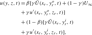 \begin{align} u(y,z,t) & = \beta [\gamma \bar {U}(x_r,y^o_r,t) + (1-\gamma ) U_{\infty } \nonumber \\[3pt] & + \gamma u'(x_r,y^o_r,z_r,t) ] \nonumber \\[3pt] & + (1-\beta ) [\gamma \bar {U}(x_r,y^i_r,t) \nonumber \\[3pt] & + \gamma u'(x_r,y^i_r,z_r,t) ], \end{align}
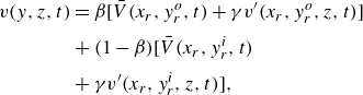 \begin{align} v(y,z,t) & = \beta [\bar {V}(x_r,y^o_r,t) + \gamma v'(x_r,y^o_r,z,t)] \nonumber \\[3pt] & + (1-\beta )[\bar {V}(x_r,y^i_r,t) \nonumber \\[3pt] & + \gamma v'(x_r,y^i_r,z,t)], \end{align}
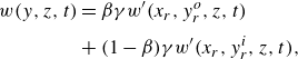 \begin{align} w(y,z,t)& = \beta \gamma w'(x_r,y^o_r,z,t) \nonumber \\[3pt] & + (1-\beta )\gamma w'(x_r,y^i_r,z,t), \end{align}
where the $\bar {(\cdot )}$
is the spanwise average through time, ‘r’ denotes the recycle plane, ‘i’ denotes the inner scale, ‘o’ denotes the outer scale. The inner scales are based on the
$\bar {(\cdot )}$
is the spanwise average through time, ‘r’ denotes the recycle plane, ‘i’ denotes the inner scale, ‘o’ denotes the outer scale. The inner scales are based on the $y^+ = yu_{\tau } /\nu$
scaling and the outer scales are based on
$y^+ = yu_{\tau } /\nu$
scaling and the outer scales are based on $\eta = y/\delta _{99}$
. Here
$\eta = y/\delta _{99}$
. Here $\beta$
is Lund’s weighting function as given in (A4), which is used to blend the inner and outer scales. The values of constants are
$\beta$
is Lund’s weighting function as given in (A4), which is used to blend the inner and outer scales. The values of constants are $a=4$
and
$a=4$
and $b=0.2$
in the following:
$b=0.2$
in the following:
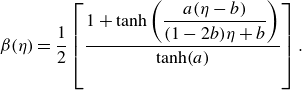 \begin{equation} \beta (\eta ) = \displaystyle\frac {1}{2} \left [\displaystyle\frac {1 + \textrm{tanh} \left ( \displaystyle\frac {a(\eta - b)}{(1-2b) \eta + b} \right )} { \textrm{tanh}(a) } \right ]. \end{equation}
The mean velocity profile is obtained by spanwise averaging at every time step and then averaging over a sliding time window. The averaging time window is initially set to $T = A \delta _{99,i}|_0/U_{\infty }$
where
$T = A \delta _{99,i}|_0/U_{\infty }$
where $A=10$
to discard the transients and then switched to
$A=10$
to discard the transients and then switched to $100$
once the transients die out. The running average,
$100$
once the transients die out. The running average,
 \begin{equation} {\mathcal{F}}(t) = \left ( 1-\frac {\Delta t}{T} \right ){\mathcal{F}}(t-\Delta t) + \frac {\Delta t}{T}f(t), \end{equation}
where $f$
is the instantaneous spanwise average. Finally, the averaging is switched to a simple running average with
$f$
is the instantaneous spanwise average. Finally, the averaging is switched to a simple running average with $T= T_0 + t -t_0$
where,
$T= T_0 + t -t_0$
where, $t$
is the time in the simulation,
$t$
is the time in the simulation, $t_0$
is the time at which the running averaging was initiated and
$t_0$
is the time at which the running averaging was initiated and $T_0$
is the value of the averaging interval used prior to
$T_0$
is the value of the averaging interval used prior to $t_0$
. This mean boundary layer velocity profile is used to evaluate the scaling parameters
$t_0$
. This mean boundary layer velocity profile is used to evaluate the scaling parameters $(\theta , \delta _{99}, u_{\tau })$
as a function of the streamwise location.
$(\theta , \delta _{99}, u_{\tau })$
as a function of the streamwise location.
In order to generate the desired turbulent inflow, the inflow parameters $u_{\tau ,i}$
,
$u_{\tau ,i}$
, $\theta _{i}$
and
$\theta _{i}$
and $\delta _{99,i}$
are specified. The value of
$\delta _{99,i}$
are specified. The value of $\theta _{i}$
is kept fixed whereas
$\theta _{i}$
is kept fixed whereas $u_{\tau ,i}$
is computed at every time step using the following, knowing the values of flow parameters at the recycling plane:
$u_{\tau ,i}$
is computed at every time step using the following, knowing the values of flow parameters at the recycling plane:
 \begin{equation} u_{\tau ,i} = u_{\tau ,r} \left ( \frac {\theta _r}{\theta _i} \right )^{(1/8)}. \end{equation}
The rescale parameter $\gamma$
is defined as
$\gamma$
is defined as
 \begin{equation} \gamma = \frac {u_{\tau ,i}}{u_{\tau ,r}} = \left ( \frac {\theta _r}{\theta _i} \right )^{(1/8)}, \end{equation}
which is used to construct velocities at the inflow plane. The constructed inflow plane velocity profiles are adjusted through a Newton–Raphson scheme to obtain $\delta _{99,i}$
.
$\delta _{99,i}$
.
A schematic of the computational domain showing the recycle–rescale method. The velocities at recycling plane ( $x=x_{rec}$
) are rescaled and prescribed to the inflow plane at each time step to generate turbulent inflow (Lund et al. Reference Lund, Wu and Squires1998).
$x=x_{rec}$
) are rescaled and prescribed to the inflow plane at each time step to generate turbulent inflow (Lund et al. Reference Lund, Wu and Squires1998).
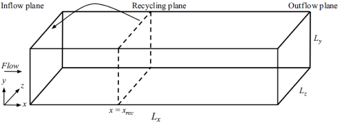
A.2. Validation
Simulations are performed for spatially developing TBL for two inflow Reynolds number, $Re_{\theta ,in} = 1410$
and
$Re_{\theta ,in} = 1410$
and $2200$
using the numerical algorithm described in (2.1). The computational domain used for simulations is a box of length
$2200$
using the numerical algorithm described in (2.1). The computational domain used for simulations is a box of length $L_x$
, width
$L_x$
, width $L_z$
and height
$L_z$
and height $L_y$
as shown in figure 20. The subscripts
$L_y$
as shown in figure 20. The subscripts $x$
,
$x$
, $y$
and
$y$
and $z$
refer to streamwise, wall-normal and spanwise directions, respectively. Flow is from the left-hand side to the right-hand side. The wall is situated at
$z$
refer to streamwise, wall-normal and spanwise directions, respectively. Flow is from the left-hand side to the right-hand side. The wall is situated at $y=0$
plane. No-slip boundary condition is applied on the wall. Convective boundary conditions are prescribed at the outflow. The boundary conditions on the top surface (
$y=0$
plane. No-slip boundary condition is applied on the wall. Convective boundary conditions are prescribed at the outflow. The boundary conditions on the top surface ( $y=L_y$
) are
$y=L_y$
) are
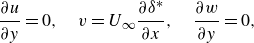 \begin{equation} \begin{aligned} \frac {\partial {u}}{\partial {y}} = 0,\quad v = U_{\infty }\frac {\partial {\delta ^*}}{\partial {x}},\quad \frac {\partial {w}}{\partial {y}} = 0, \end{aligned} \end{equation}
where $\delta ^*$
is the boundary layer displacement thickness and
$\delta ^*$
is the boundary layer displacement thickness and $U_\infty$
is the free stream velocity. At every time step,
$U_\infty$
is the free stream velocity. At every time step, $\delta ^*$
is computed from the mean velocity field as a function of
$\delta ^*$
is computed from the mean velocity field as a function of $x$
and then the derivative
$x$
and then the derivative ${\partial {\delta ^*}}/{\partial {x}}$
is computed as an average slope, whose value is usually small.
${\partial {\delta ^*}}/{\partial {x}}$
is computed as an average slope, whose value is usually small.
The $\theta _{in}$
is kept fixed at 0.1 for both cases. The location of recycling plane has to be sufficiently far away from the inflow and outflow to avoid any unphysical behaviour. The computational grid is uniform in streamwise (
$\theta _{in}$
is kept fixed at 0.1 for both cases. The location of recycling plane has to be sufficiently far away from the inflow and outflow to avoid any unphysical behaviour. The computational grid is uniform in streamwise ( $x$
) and spanwise (
$x$
) and spanwise ( $z$
) direction with a clustering near wall in wall-normal (
$z$
) direction with a clustering near wall in wall-normal ( $y$
) direction to resolve fine near-wall flow structures. The details of the simulations are listed in table 4.
$y$
) direction to resolve fine near-wall flow structures. The details of the simulations are listed in table 4.
Domain size and grid distribution for the DNS. Here, $L_x$
,
$L_x$
, $L_y$
and
$L_y$
and $L_z$
are the domain size in the streamwise, wall-normal and spanwise directions, respectively; and
$L_z$
are the domain size in the streamwise, wall-normal and spanwise directions, respectively; and $N_x$
,
$N_x$
, $N_y$
and
$N_y$
and $N_z$
are the number of control volumes in those directions, respectively. Here
$N_z$
are the number of control volumes in those directions, respectively. Here $x_{rec}$
is the location of the recycling plane and
$x_{rec}$
is the location of the recycling plane and $\theta _{in}$
is the prescribed momentum thickness at the inflow. Here
$\theta _{in}$
is the prescribed momentum thickness at the inflow. Here $Re_{\theta ,in}$
is the prescribed inflow Reynolds number based on
$Re_{\theta ,in}$
is the prescribed inflow Reynolds number based on $\theta _{in}$
.
$\theta _{in}$
.
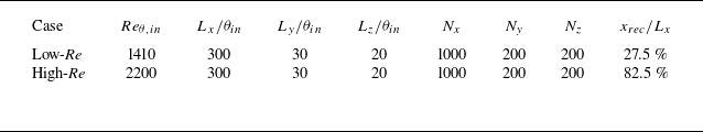
Low-Re: mean and second-order velocity statistics at $Re_{\theta } = 1420$
(
$Re_{\theta } = 1420$
( $a,b$
), 1551 (
$a,b$
), 1551 ( $c,d$
) and 1968 (
$c,d$
) and 1968 ( $e,f$
). Symbols are DNS from Schlatter & Örlü (Reference Schlatter and Örlü2010) (
$e,f$
). Symbols are DNS from Schlatter & Örlü (Reference Schlatter and Örlü2010) ( $a,b$
) and Jiménez et al. (Reference Jiménez, Hoyas, Simens and Mizuno2010) (
$a,b$
) and Jiménez et al. (Reference Jiménez, Hoyas, Simens and Mizuno2010) ( $c{-}f$
).
$c{-}f$
).
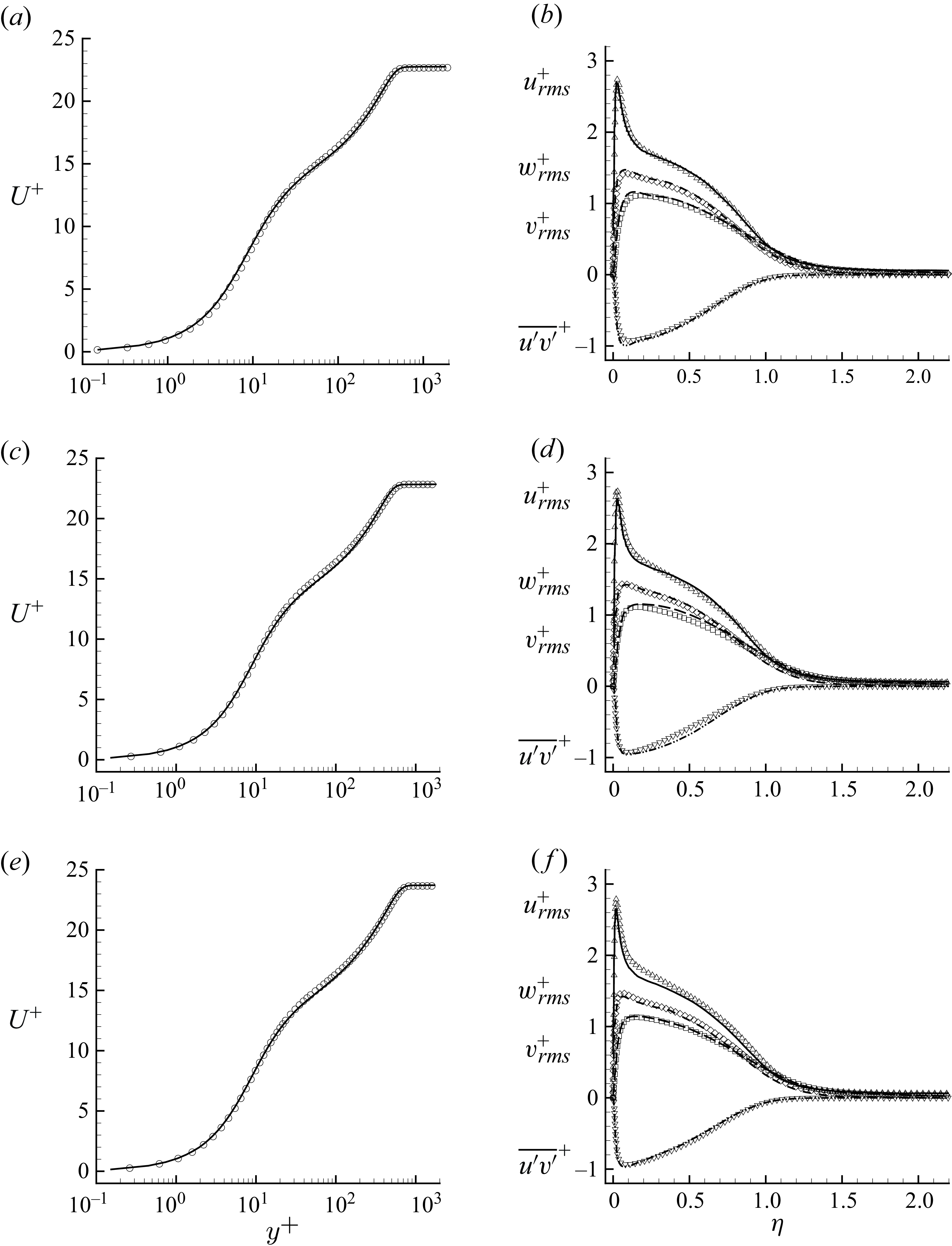
High-Re: mean and second-order velocity statistics at $Re_{\theta } = 2540$
(
$Re_{\theta } = 2540$
( $a,b$
) and 3032 (
$a,b$
) and 3032 ( $c,d$
). Symbols are DNS from Schlatter & Örlü (Reference Schlatter and Örlü2010).
$c,d$
). Symbols are DNS from Schlatter & Örlü (Reference Schlatter and Örlü2010).
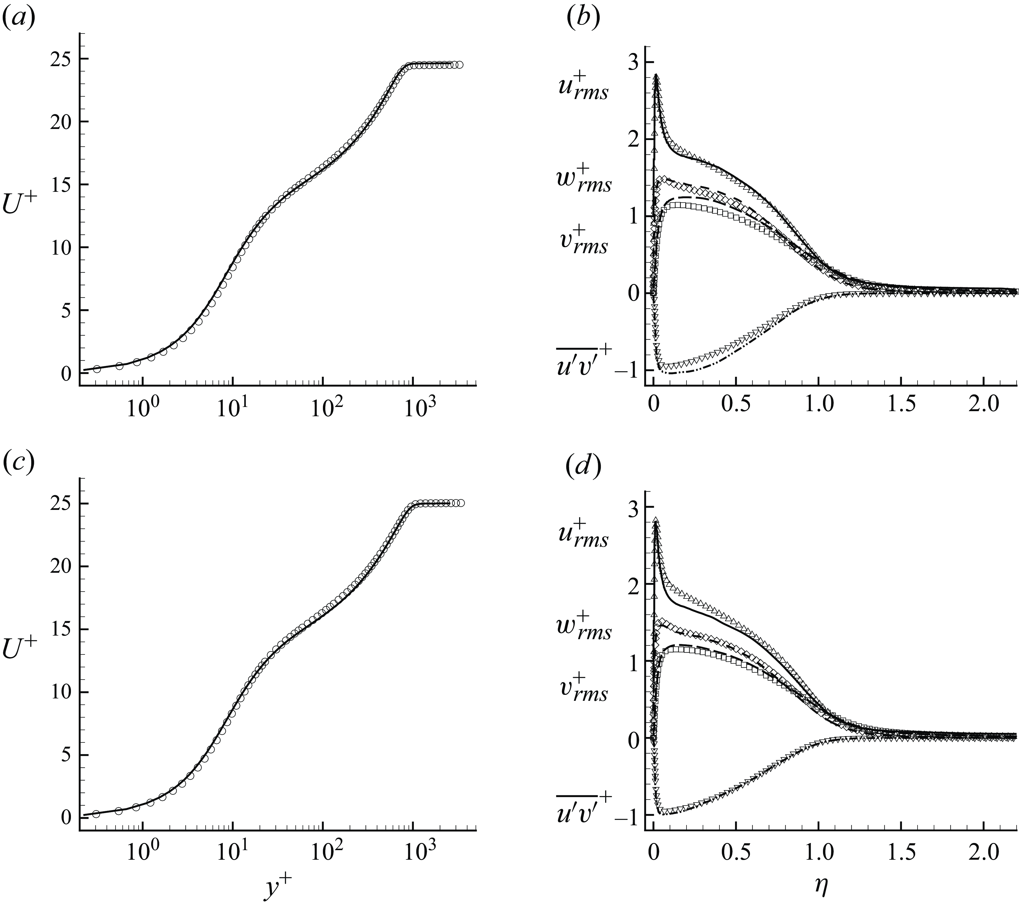
The profiles for mean velocity and second-order statistics from the low-Re case are compared with the DNS results at $Re_{\theta }=1420$
(Schlatter & Örlü Reference Schlatter and Örlü2010),
$Re_{\theta }=1420$
(Schlatter & Örlü Reference Schlatter and Örlü2010), $Re_{\theta }=1551$
and
$Re_{\theta }=1551$
and $Re_{\theta }=1968$
(Jiménez et al. Reference Jiménez, Hoyas, Simens and Mizuno2010) as shown in figure 21. The profiles are extracted at three streamwise locations for the low-Re case and two streamwise locations for the high-Re case (see table 4). The extracted profiles from the high-Re case are compared with DNS results at
$Re_{\theta }=1968$
(Jiménez et al. Reference Jiménez, Hoyas, Simens and Mizuno2010) as shown in figure 21. The profiles are extracted at three streamwise locations for the low-Re case and two streamwise locations for the high-Re case (see table 4). The extracted profiles from the high-Re case are compared with DNS results at $Re_{\theta }=2540$
and
$Re_{\theta }=2540$
and $Re_{\theta }=3032$
(Schlatter & Örlü Reference Schlatter and Örlü2010) as shown in figure 22. The results from both cases show very good agreement with the DNS data available in the literature. The corresponding grid details are listed in table 5. Thus, the simulation method to generate a ZPG TBL of desired properties can be considered validated.
$Re_{\theta }=3032$
(Schlatter & Örlü Reference Schlatter and Örlü2010) as shown in figure 22. The results from both cases show very good agreement with the DNS data available in the literature. The corresponding grid details are listed in table 5. Thus, the simulation method to generate a ZPG TBL of desired properties can be considered validated.
Grid resolution at different streamwise locations in wall units. The streamwise ( $x$
) and spanwise (
$x$
) and spanwise ( $z$
) directions have uniform grid distribution whereas the grid is clustered near wall in wall-normal (
$z$
) directions have uniform grid distribution whereas the grid is clustered near wall in wall-normal ( $y$
) direction. Here,
$y$
) direction. Here, $y^{+}$
is the first cell size near wall. The low-Re and high-Re are cases with
$y^{+}$
is the first cell size near wall. The low-Re and high-Re are cases with $Re_{\theta ,in}=1410$
and 2200, respectively.
$Re_{\theta ,in}=1410$
and 2200, respectively.
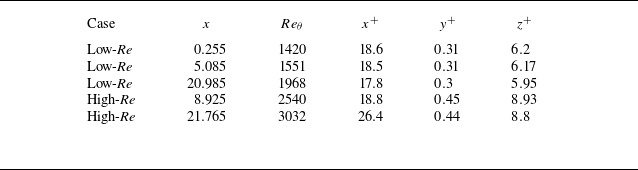
Appendix B. Sensitivity to domain size
The streamwise variation of $U_e$
$U_e$ $(a)$
and
$(a)$
and $u_{\tau }$ $(b)$
velocities are compared between Domain1 (
$(b)$
velocities are compared between Domain1 ( $L_z = 3$
) and Domain 2 (
$L_z = 3$
) and Domain 2 ( $L_z=6$
).
$L_z=6$
).
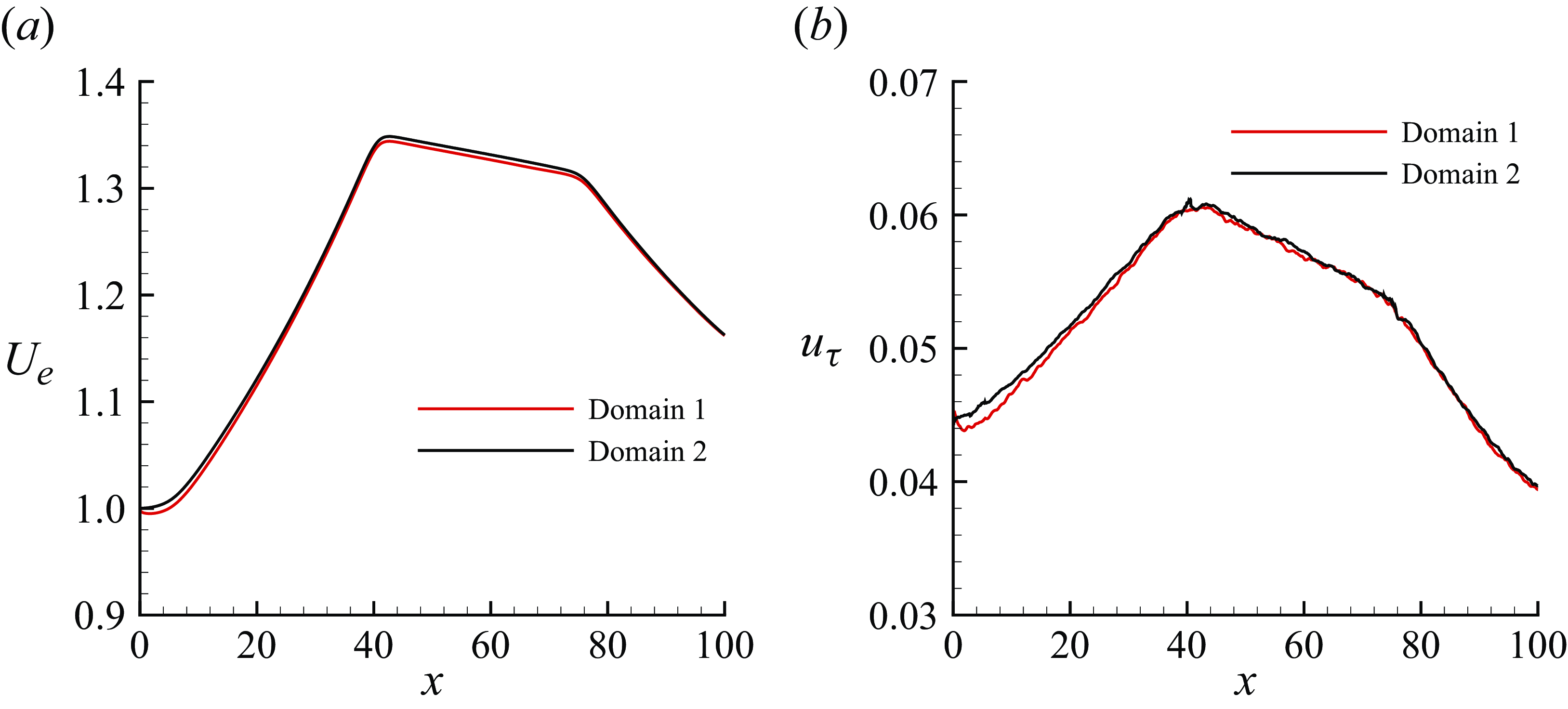
Simulations were performed on two different computational domains, which differed only in the spanwise length ( $L_z$
). Domain 1 had
$L_z$
). Domain 1 had $L_z = 3 \delta _{99}$
, where
$L_z = 3 \delta _{99}$
, where $\delta _{99} =1$
is the boundary layer thickness at the inflow plane. Domain 2 had double the size in spanwise direction. Both computational domains had identical grid resolutions. Figure 23 shows the streamwise variation of
$\delta _{99} =1$
is the boundary layer thickness at the inflow plane. Domain 2 had double the size in spanwise direction. Both computational domains had identical grid resolutions. Figure 23 shows the streamwise variation of $U_e$
and
$U_e$
and $u_{\tau }$
for the two cases. Figure 24 shows the wall-normal profiles of Reynolds shear stress components at Stations 6 and 12 for the two cases. Note that the values are not normalised for direct comparison. Some difference can be observed at Station 12 in the streamwise Reynolds shear stress. The mean velocity profiles at these stations (not shown here) were identical for the two cases. Overall, the results suggest that Domain 2 was sufficiently wide for the present flow problem. Even wider domain is not expected to make any appreciable difference in the results shown in this work.
$u_{\tau }$
for the two cases. Figure 24 shows the wall-normal profiles of Reynolds shear stress components at Stations 6 and 12 for the two cases. Note that the values are not normalised for direct comparison. Some difference can be observed at Station 12 in the streamwise Reynolds shear stress. The mean velocity profiles at these stations (not shown here) were identical for the two cases. Overall, the results suggest that Domain 2 was sufficiently wide for the present flow problem. Even wider domain is not expected to make any appreciable difference in the results shown in this work.
The wall-normal profiles of Reynolds stress components are compared between Domain1 ( $L_z = 3$
) and Domain 2 (
$L_z = 3$
) and Domain 2 ( $L_z = 6$
) at Station 6
$L_z = 6$
) at Station 6 $(a)$
and Station 12
$(a)$
and Station 12 $(b)$
.
$(b)$
.
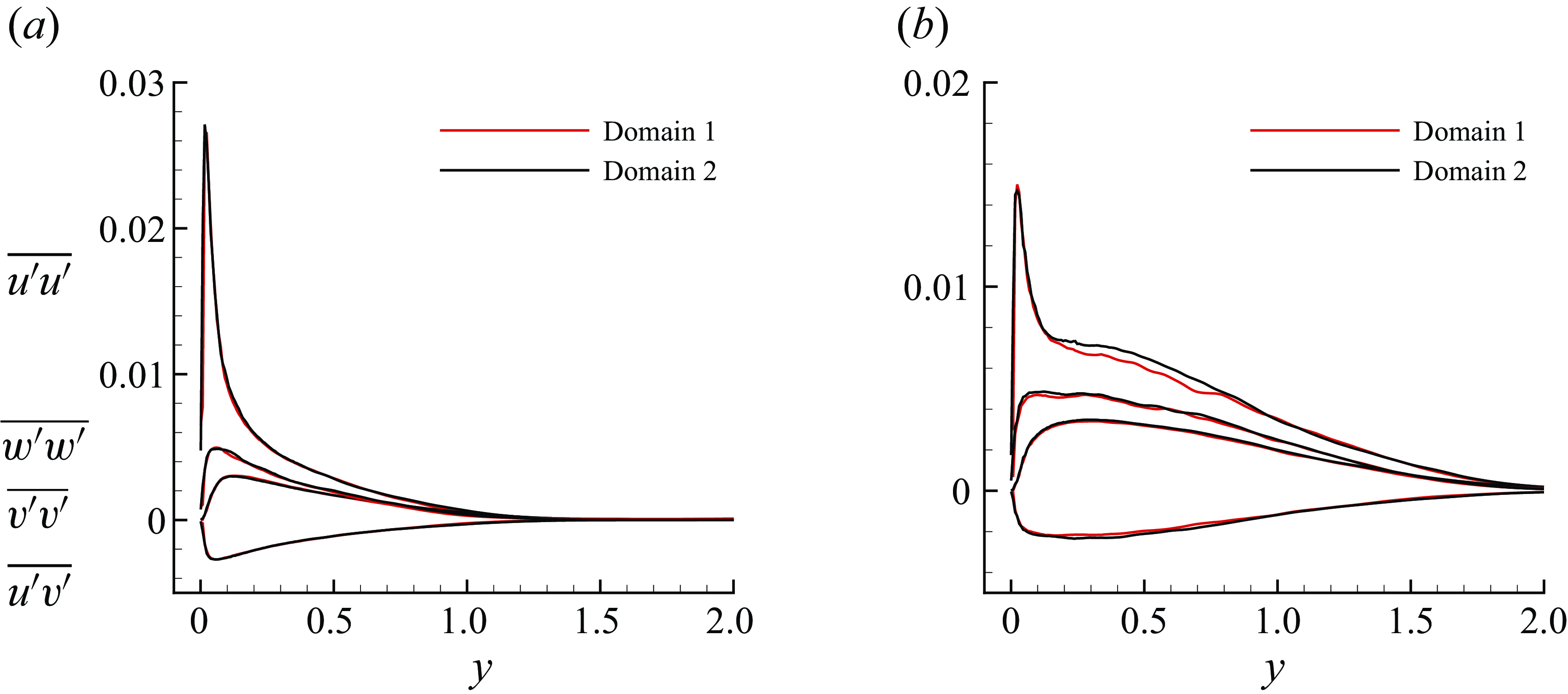
Appendix C. Additional profile comparisons
The profile comparisons with the reference data at Stations 2–5, 7, 8, 10 and 11 are shown for the mean velocity defect (figure 25), the r.m.s. of streamwise (figure 26) and wall-normal (figure 27) velocity fluctuations, and the Reynolds shear stress (figure 28). All the profiles are normalised by the local mean streamwise velocity in the free stream.
Mean velocity defect profiles (lines) are compared with the reference data (symbols) of Volino (Reference Volino2020a
) at Stations 2–5 $(a-d)$
, Stations 7–8
$(a-d)$
, Stations 7–8 $(e,f)$
and Stations 10–11
$(e,f)$
and Stations 10–11 $(g,h)$
.
$(g,h)$
.
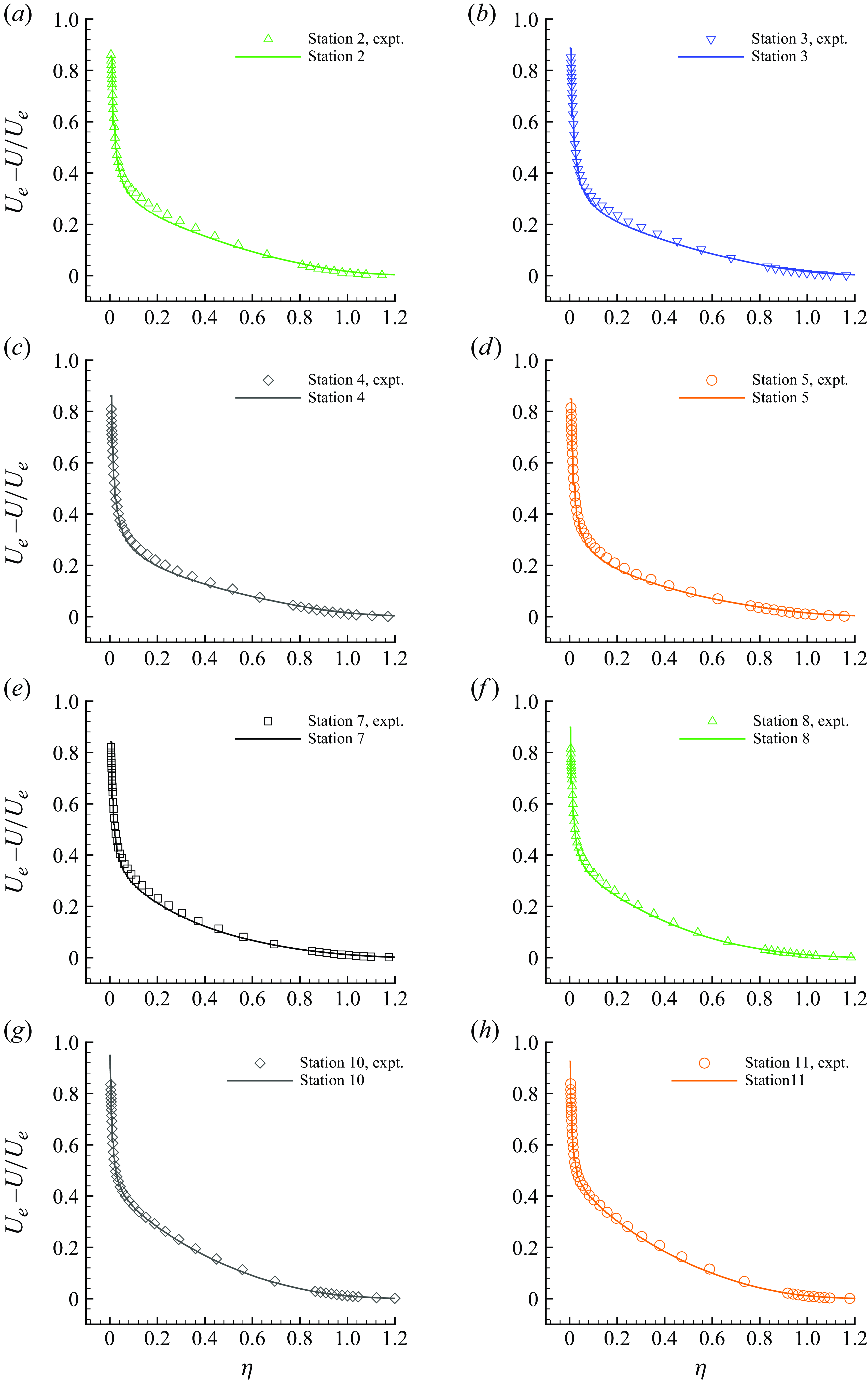
The r.m.s. of streamwise velocity fluctuations (lines) are compared with the reference data (symbols) of Volino (Reference Volino2020a ) at the same stations as figure 25.
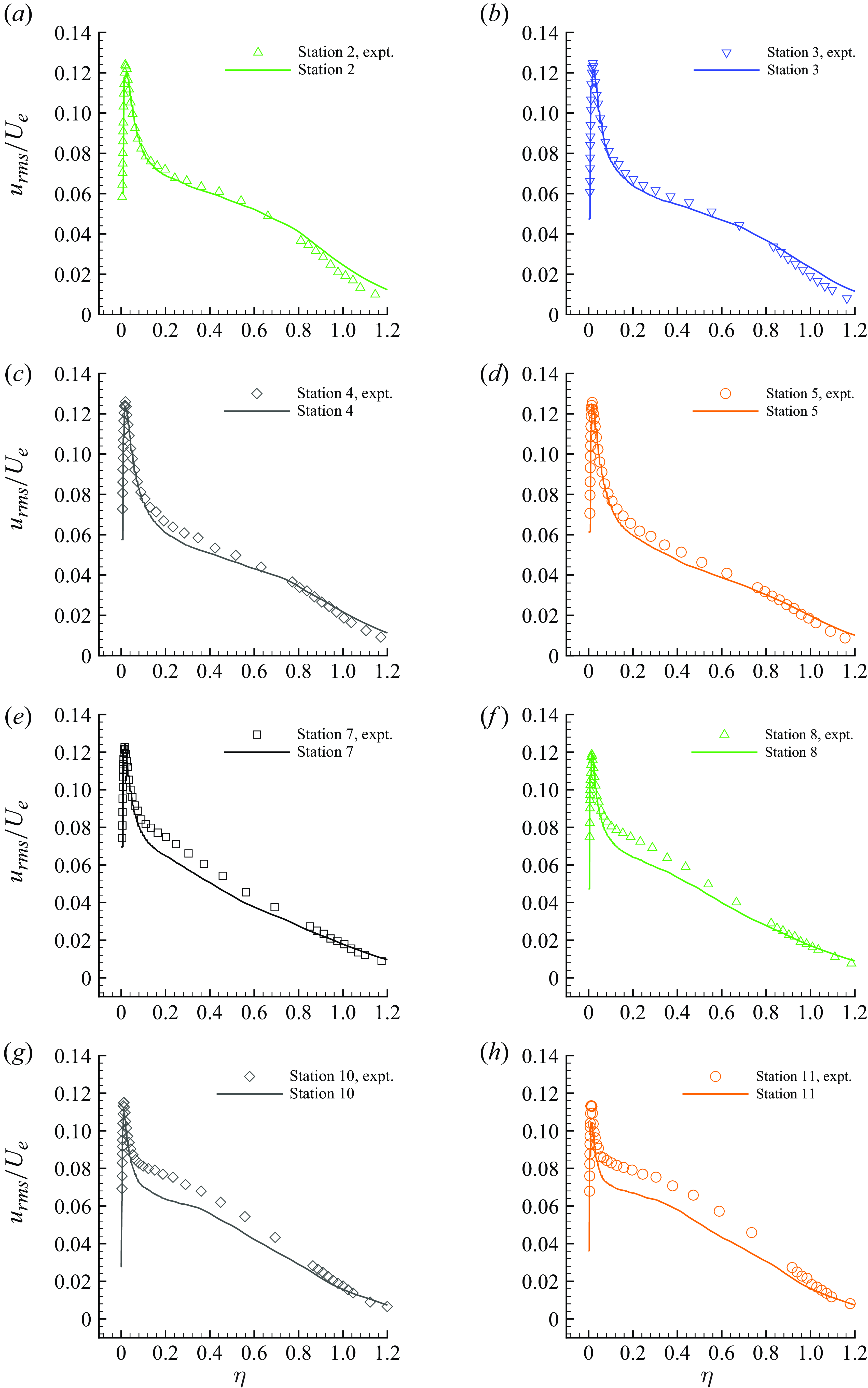
The r.m.s. of wall-normal velocity fluctuations (lines) are compared with the reference data (symbols) of Volino (Reference Volino2020a ) at the same stations as figure 25.
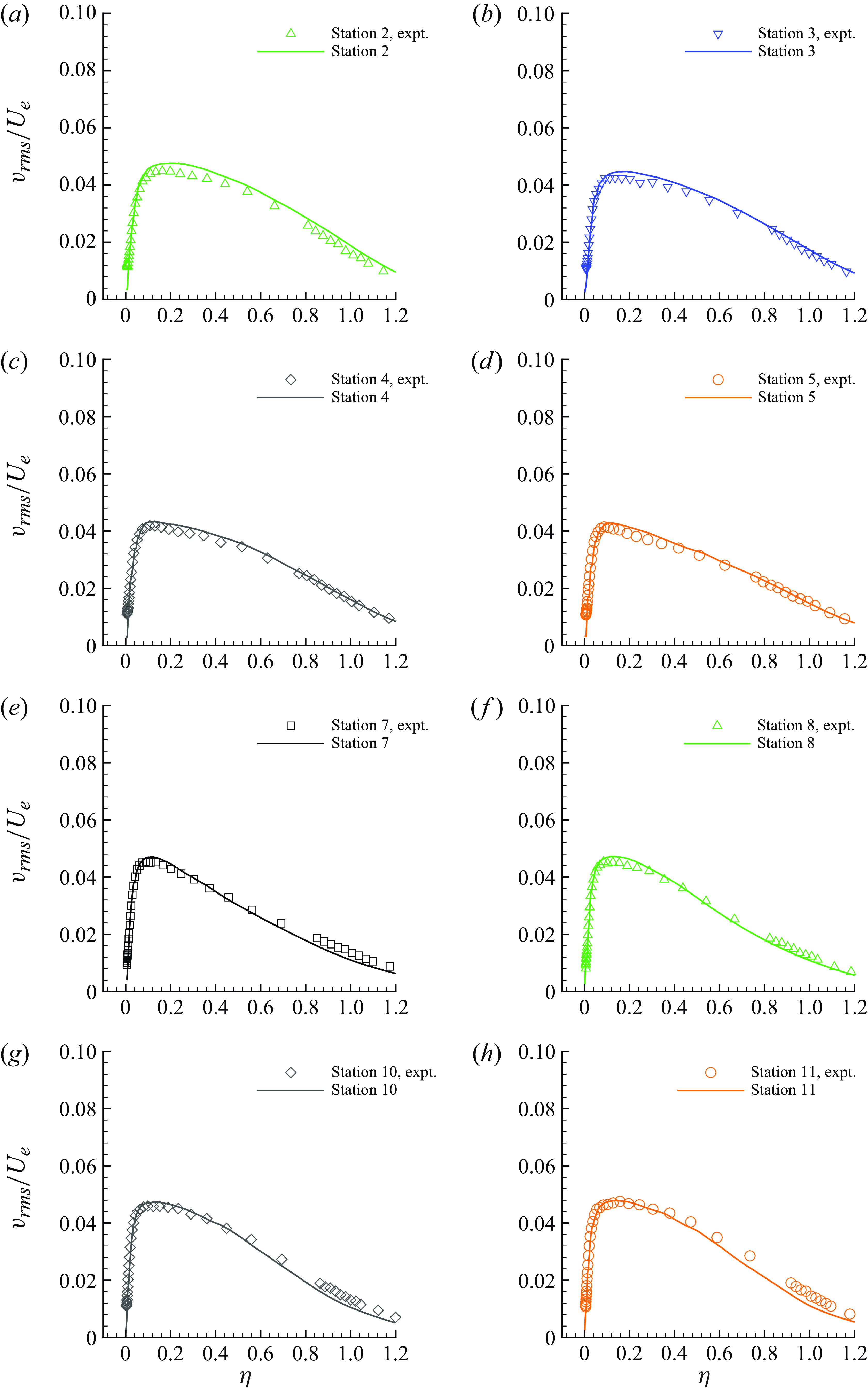
Reynolds shear stress profiles (lines) are compared with the reference data (symbols) of Volino (Reference Volino2020a ) at the same stations as figure 25.
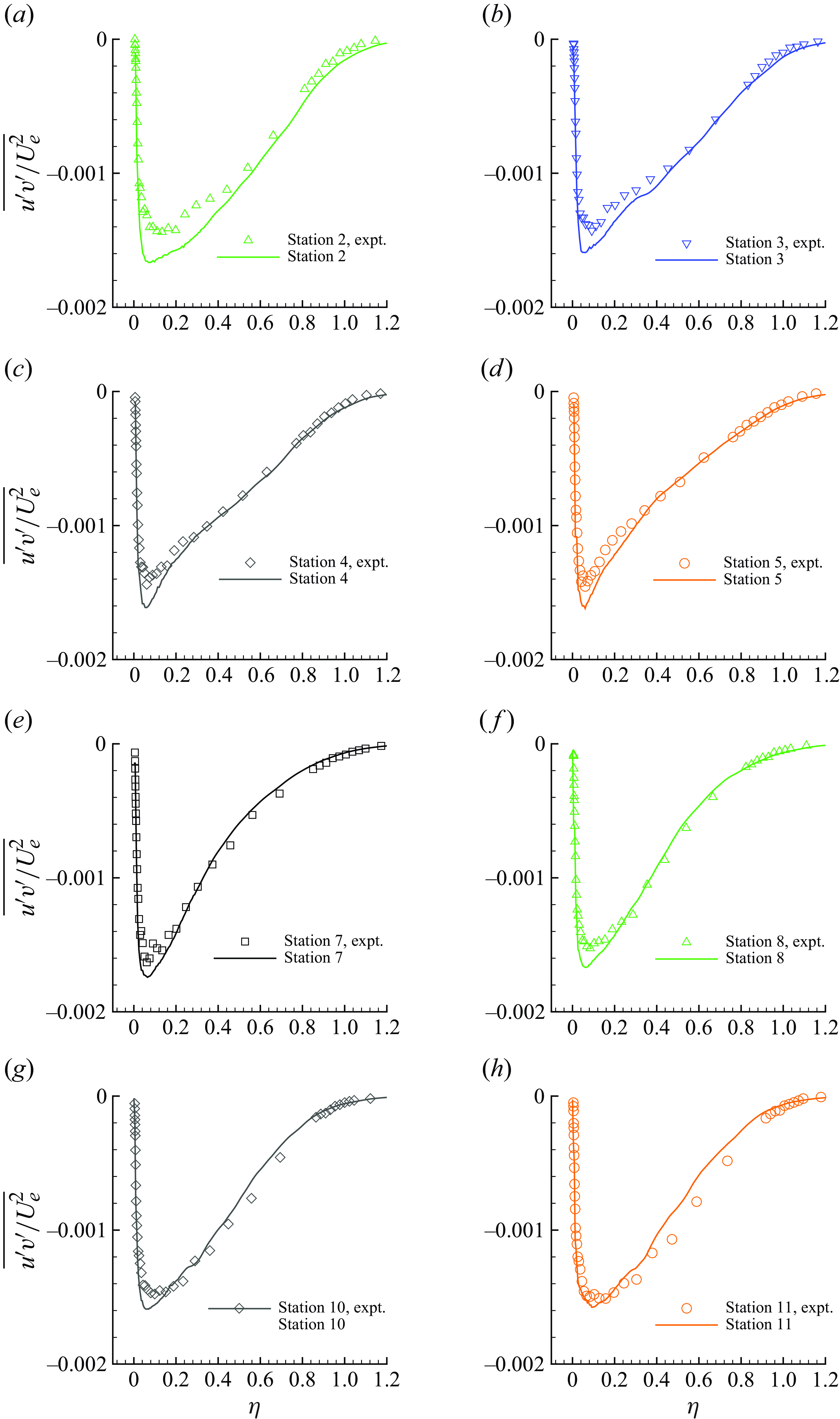


 Open access