


1. Introduction
Studying the behaviour of the Nusselt number ( $\textit{Nu}$
) in high-Rayleigh-number (
$\textit{Nu}$
) in high-Rayleigh-number ( $ \textit{Ra} $
) natural convection has attracted considerable attention from both applied and fundamental fluid dynamics perspectives. The emergence of a power-law relationship
$ \textit{Ra} $
) natural convection has attracted considerable attention from both applied and fundamental fluid dynamics perspectives. The emergence of a power-law relationship $\textit{Nu} \propto Ra^{\beta }$
in experimental data, with the exponent
$\textit{Nu} \propto Ra^{\beta }$
in experimental data, with the exponent $\beta$
being approximately 1/3 over a broad range of
$\beta$
being approximately 1/3 over a broad range of $ \textit{Ra} $
, has long been empirically known. In modern convection research, the scaling law
$ \textit{Ra} $
, has long been empirically known. In modern convection research, the scaling law $\textit{Nu} \propto Ra^{1/3}$
is known as the classical scaling and often serves as a baseline for organising experimental data.
$\textit{Nu} \propto Ra^{1/3}$
is known as the classical scaling and often serves as a baseline for organising experimental data.
In Rayleigh–Bénard convection, the classical scaling appears in experiments when $ \textit{Ra} $
reaches around
$ \textit{Ra} $
reaches around $10^9$
(Chavanne et al. Reference Chavanne, Chilla, Chabaud, Castaing and Hebral2001; Funfschilling et al. Reference Funfschilling, Brown, Nikolaenko and Ahlers2005; Niemela & Sreenivasan Reference Niemela and Sreenivasan2006) in terms of the Rayleigh number defined as
$10^9$
(Chavanne et al. Reference Chavanne, Chilla, Chabaud, Castaing and Hebral2001; Funfschilling et al. Reference Funfschilling, Brown, Nikolaenko and Ahlers2005; Niemela & Sreenivasan Reference Niemela and Sreenivasan2006) in terms of the Rayleigh number defined as $Ra=g\alpha H^3\Delta T/\nu \kappa$
. Here,
$Ra=g\alpha H^3\Delta T/\nu \kappa$
. Here, $H$
is the distance between the walls,
$H$
is the distance between the walls, $\Delta T$
is their temperature difference,
$\Delta T$
is their temperature difference, $\alpha$
is the coefficient of thermal expansion of the fluid,
$\alpha$
is the coefficient of thermal expansion of the fluid, $g$
is the gravitational constant,
$g$
is the gravitational constant, $\nu$
is the kinematic viscosity and
$\nu$
is the kinematic viscosity and $\kappa$
is the thermal diffusivity. Experiments have traditionally been the primary research method for studying the heat transport in this flow, with other major approaches including direct numerical simulations (DNS), upper bound theory and modelling. Lohse & Shishkina (Reference Lohse and Shishkina2024) provide a comprehensive and up-to-date review of them, including a summary of currently available major experimental data (see figure 11a of that paper). At
$\kappa$
is the thermal diffusivity. Experiments have traditionally been the primary research method for studying the heat transport in this flow, with other major approaches including direct numerical simulations (DNS), upper bound theory and modelling. Lohse & Shishkina (Reference Lohse and Shishkina2024) provide a comprehensive and up-to-date review of them, including a summary of currently available major experimental data (see figure 11a of that paper). At $Ra\gtrsim O(10^{11})$
, some of these data exhibit the so-called ultimate regime, with an exponent
$Ra\gtrsim O(10^{11})$
, some of these data exhibit the so-called ultimate regime, with an exponent $\beta \gt 1/3$
. Capturing this regime in DNS remains challenging, as it requires computational domains that are large enough. A mathematically rigorous upper bound of the form
$\beta \gt 1/3$
. Capturing this regime in DNS remains challenging, as it requires computational domains that are large enough. A mathematically rigorous upper bound of the form $\textit{Nu}\propto Ra^{1/2}$
can be derived (Howard Reference Howard1963; Doering & Constantin Reference Doering and Constantin1996; Plasting & Kerswell Reference Plasting and Kerswell2003). However, since upper bound theory relies solely on energy balance, the resulting estimate is rather crude. The development of models incorporating physical insight to describe the trends observed in experiments has therefore been an active area of research (Grossmann & Lohse Reference Grossmann and Lohse2000; Kawano et al. Reference Kawano, Motoki, Shimizu and Kawahara2021; Shishkina & Lohse Reference Shishkina and Lohse2024).
$\textit{Nu}\propto Ra^{1/2}$
can be derived (Howard Reference Howard1963; Doering & Constantin Reference Doering and Constantin1996; Plasting & Kerswell Reference Plasting and Kerswell2003). However, since upper bound theory relies solely on energy balance, the resulting estimate is rather crude. The development of models incorporating physical insight to describe the trends observed in experiments has therefore been an active area of research (Grossmann & Lohse Reference Grossmann and Lohse2000; Kawano et al. Reference Kawano, Motoki, Shimizu and Kawahara2021; Shishkina & Lohse Reference Shishkina and Lohse2024).
This study takes a different approach from those mentioned above and is based on the computation of steady solutions and their large- $ \textit{Ra} $
asymptotic analysis. The idea of investigating
$ \textit{Ra} $
asymptotic analysis. The idea of investigating $\textit{Nu}$
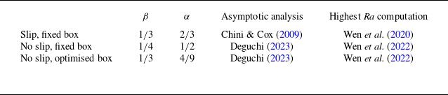
scaling using simple solutions of the governing equations, now known as exact coherent states (ECS), has a long history in natural convection. In the early days of numerical natural convection studies, two-dimensional (2-D) stationary roll cells were used to examine the scaling behaviour (Pillow Reference Pillow1952; Malkus & Veronis Reference Malkus and Veronis1958; Herring Reference Herring1963; Robinson Reference Robinson1967; Wesseling Reference Wesseling1969). More recently, asymptotic and numerical analyses of the roll cells at large Rayleigh numbers, as summarised in table 1, have provided deeper insights, building on the gradual accumulation of past discoveries. The exponent
$\textit{Nu}$
scaling using simple solutions of the governing equations, now known as exact coherent states (ECS), has a long history in natural convection. In the early days of numerical natural convection studies, two-dimensional (2-D) stationary roll cells were used to examine the scaling behaviour (Pillow Reference Pillow1952; Malkus & Veronis Reference Malkus and Veronis1958; Herring Reference Herring1963; Robinson Reference Robinson1967; Wesseling Reference Wesseling1969). More recently, asymptotic and numerical analyses of the roll cells at large Rayleigh numbers, as summarised in table 1, have provided deeper insights, building on the gradual accumulation of past discoveries. The exponent $\beta$
depends on the boundary conditions on the walls (Robinson Reference Robinson1967). For no-slip walls, achieving the classical scaling requires optimising the computational box to maximise
$\beta$
depends on the boundary conditions on the walls (Robinson Reference Robinson1967). For no-slip walls, achieving the classical scaling requires optimising the computational box to maximise $\textit{Nu}$
(Waleffe, Boonkasame & Smith Reference Waleffe, Boonkasame and Smith2015; Sondak, Smith & Waleffe Reference Sondak, Smith and Waleffe2015; Wen, Goluskin & Doering Reference Wen, Goluskin and Doering2022). A large-
$\textit{Nu}$
(Waleffe, Boonkasame & Smith Reference Waleffe, Boonkasame and Smith2015; Sondak, Smith & Waleffe Reference Sondak, Smith and Waleffe2015; Wen, Goluskin & Doering Reference Wen, Goluskin and Doering2022). A large- $ \textit{Ra} $
asymptotic theory by Deguchi (Reference Deguchi2023) adds further evidence that the exponent
$ \textit{Ra} $
asymptotic theory by Deguchi (Reference Deguchi2023) adds further evidence that the exponent $\beta$
of the optimised 2-D roll cell is indeed
$\beta$
of the optimised 2-D roll cell is indeed $1/3$
.
$1/3$
.
Scaling of the 2-D roll-cell solution. The exponents $\beta$
and
$\beta$
and $\alpha$
appearing in the power laws
$\alpha$
appearing in the power laws $\textit{Nu} \propto Ra^{\beta }$
and
$\textit{Nu} \propto Ra^{\beta }$
and $\textit{Re} \propto Ra^{\alpha }$
are shown. The definitions of the Nusselt number
$\textit{Re} \propto Ra^{\alpha }$
are shown. The definitions of the Nusselt number $\textit{Nu}$
and the wind Reynolds number
$\textit{Nu}$
and the wind Reynolds number $\textit{Re}$
are given in section 2.
$\textit{Re}$
are given in section 2.

The motivation for studying ECS may not be immediately apparent, as ECS are far simpler than observed turbulent flows. To clarify this, let us define $\aleph$
as the maximum Nusselt number attainable by all statistically steady states. This mathematically well-defined quantity is of central importance in the study of natural convection, as it reveals the fundamental limits of heat transfer permitted by the governing equations. The exact value of
$\aleph$
as the maximum Nusselt number attainable by all statistically steady states. This mathematically well-defined quantity is of central importance in the study of natural convection, as it reveals the fundamental limits of heat transfer permitted by the governing equations. The exact value of $\aleph$
is unknown, but it is expected to be bounded above by the best known result from the upper bound theory, denoted
$\aleph$
is unknown, but it is expected to be bounded above by the best known result from the upper bound theory, denoted $\aleph _{\textit{UB}}$
; this result is due to Plasting & Kerswell (Reference Plasting and Kerswell2003) for finite Prandtl numbers; see the review by Lohse & Shishkina (Reference Lohse and Shishkina2024). The lower bound,
$\aleph _{\textit{UB}}$
; this result is due to Plasting & Kerswell (Reference Plasting and Kerswell2003) for finite Prandtl numbers; see the review by Lohse & Shishkina (Reference Lohse and Shishkina2024). The lower bound, $\aleph _{\textit{LB}}$
, on the other hand, can be estimated by compiling available data from experiments, DNS and ECS computations. Wen et al. (Reference Wen, Goluskin and Doering2022) argued that their 2-D roll-cell solutions up to
$\aleph _{\textit{LB}}$
, on the other hand, can be estimated by compiling available data from experiments, DNS and ECS computations. Wen et al. (Reference Wen, Goluskin and Doering2022) argued that their 2-D roll-cell solutions up to $Ra=10^{14}$
yield Nusselt numbers that exceed all available experimental and DNS results; this represent the present value of
$Ra=10^{14}$
yield Nusselt numbers that exceed all available experimental and DNS results; this represent the present value of $\aleph _{\textit{LB}}$
. The ECS thus potentially offer a powerful and promising approach to better estimate
$\aleph _{\textit{LB}}$
. The ECS thus potentially offer a powerful and promising approach to better estimate $\aleph \in [\aleph _{\textit{LB}}, \aleph _{\textit{UB}}]$
.
$\aleph \in [\aleph _{\textit{LB}}, \aleph _{\textit{UB}}]$
.
Our interest lies specifically in 3-D steady ECS that yield the largest possible Nusselt number in the Rayleigh–Bénard problem. Roll cells are arguably overly idealised ECS, and efforts to analyse 3-D steady solutions have previously been made, for example, by Koschmieder (Reference Koschmieder1974) and Golubitsky, Swift & Knobloch (Reference Golubitsky, Swift and Knobloch1984). Depending on how the eigenfunctions are superimposed near the linear critical point (Chandrasekhar Reference Chandrasekhar1961), convection patterns resembling squares and hexagons, often observed in experiments, are obtained (see figure 1
a,b). Yet, these solutions have not been extended to $Ra=O(10^9)$
. Exploring 3-D ECS at higher Rayleigh numbers is difficult even with modern computational power. Thus, we make use of high-
$Ra=O(10^9)$
. Exploring 3-D ECS at higher Rayleigh numbers is difficult even with modern computational power. Thus, we make use of high- $ \textit{Ra} $
asymptotic analysis, taking advantage of the relatively simple structure of the ECS.
$ \textit{Ra} $
asymptotic analysis, taking advantage of the relatively simple structure of the ECS.
Steady ECS of Rayleigh–Bénard convection. The colour maps in (a) and (b) represent the temperature fields at $Ra=10^6$
of the square and hexagon, respectively. The data are taken from a
$Ra=10^6$
of the square and hexagon, respectively. The data are taken from a $2L\times 2L$
region near the bottom hot wall (
$2L\times 2L$
region near the bottom hot wall ( $z=L/4$
), where the
$z=L/4$
), where the $x$
-period
$x$
-period $L$
is optimised. (c) Nusselt number
$L$
is optimised. (c) Nusselt number $\textit{Nu}$
as a function of
$\textit{Nu}$
as a function of $ \textit{Ra} $
. The solid blue and red lines represent the square and hexagon in a fixed box size (
$ \textit{Ra} $
. The solid blue and red lines represent the square and hexagon in a fixed box size ( $L=\pi /2$
). The filled symbols are solutions where the box size is optimised to maximise
$L=\pi /2$
). The filled symbols are solutions where the box size is optimised to maximise $\textit{Nu}$
. The open symbols are from laboratory experiments on water convection by Rossby (Reference Rossby1969) and Funfschilling et al. (Reference Funfschilling, Brown, Nikolaenko and Ahlers2005). Crosses denote data from helium gas experiments reported in Niemela & Sreenivasan (Reference Niemela and Sreenivasan2006). The black solid line shows the classical scaling
$\textit{Nu}$
. The open symbols are from laboratory experiments on water convection by Rossby (Reference Rossby1969) and Funfschilling et al. (Reference Funfschilling, Brown, Nikolaenko and Ahlers2005). Crosses denote data from helium gas experiments reported in Niemela & Sreenivasan (Reference Niemela and Sreenivasan2006). The black solid line shows the classical scaling $\textit{Nu}\propto Ra^{1/3}$
. The orange dot-dashed line is the upper bound
$\textit{Nu}\propto Ra^{1/3}$
. The orange dot-dashed line is the upper bound $\textit{Nu}-1=0.02634Ra^{1/2}$
established by Plasting & Kerswell (Reference Plasting and Kerswell2003).
$\textit{Nu}-1=0.02634Ra^{1/2}$
established by Plasting & Kerswell (Reference Plasting and Kerswell2003).

In this paper, we clearly distinguish between asymptotic analysis and modelling approaches, whose objectives are fundamentally different. Modelling primarily aims to reproduce experimental $\textit{Nu}$
data. A seminal reference for derivation of the classical scaling is Malkus (Reference Malkus1954), where heat transport is maximised under certain assumptions. However, as he himself acknowledges in the paper, the scaling estimation relies on too many modelling assumptions. In the same year, Priestley (Reference Priestley1954) independently derived the same scaling, but his derivation was not based on the Navier–Stokes equations. Many models were subsequently proposed, and the historical progress of these, extending to the latest studies, can be found in Lohse & Shishkina (Reference Lohse and Shishkina2024). The recent model by Shishkina & Lohse (Reference Shishkina and Lohse2024), derived from physical insights into turbulence, successfully captures the available experimental data over a wide range of
$\textit{Nu}$
data. A seminal reference for derivation of the classical scaling is Malkus (Reference Malkus1954), where heat transport is maximised under certain assumptions. However, as he himself acknowledges in the paper, the scaling estimation relies on too many modelling assumptions. In the same year, Priestley (Reference Priestley1954) independently derived the same scaling, but his derivation was not based on the Navier–Stokes equations. Many models were subsequently proposed, and the historical progress of these, extending to the latest studies, can be found in Lohse & Shishkina (Reference Lohse and Shishkina2024). The recent model by Shishkina & Lohse (Reference Shishkina and Lohse2024), derived from physical insights into turbulence, successfully captures the available experimental data over a wide range of $ \textit{Ra} $
and
$ \textit{Ra} $
and $\textit{Pr}$
.
$\textit{Pr}$
.
On the other hand, the central focus of the asymptotic approach is to verify that the proposed scaling laws are fully consistent with the governing equations. What distinguishes asymptotic analysis from modelling is that it requires explicitly formulating perturbation expansions of the physical quantities and substituting them into the governing equations. At the very least, the leading-order system must retain sufficient complexity, which can only be achieved through a careful choice of expansion. Once a consistent asymptotic expansion is obtained, it can completely reveal the behaviour of solutions in extreme parameter limits without further numerical computation, as illustrated by Bender & Orszag (Reference Bender and Orszag1978) through simple ordinary differential equation examples. Such analysis remains out of reach in fully turbulent regime; in fact, even the seemingly straightforward question of whether the Nusselt number in turbulent flows can be expressed as a simple function of $ \textit{Ra} $
presents a highly non-trivial mathematical challenge in asymptotic analysis.
$ \textit{Ra} $
presents a highly non-trivial mathematical challenge in asymptotic analysis.
The aim of this paper is to fully elucidate the high- $ \textit{Ra} $
scaling of the velocity and temperature fields of 3-D nonlinear convective cells using asymptotic analysis, even if the results are restricted to ECS. When we use the term scaling, our concern is with the asymptotic behaviour of the flow in the high-
$ \textit{Ra} $
scaling of the velocity and temperature fields of 3-D nonlinear convective cells using asymptotic analysis, even if the results are restricted to ECS. When we use the term scaling, our concern is with the asymptotic behaviour of the flow in the high- $ \textit{Ra} $
limit, rather than with interpreting turbulent data. As shown in table 1, whether the classical scaling can be derived from asymptotic analysis for 3-D convection cells with no-slip boundary conditions remains an open question. Our study resolves this problem by extending the asymptotic theory developed in Deguchi (Reference Deguchi2023). We shall see that the theory describes the asymptotic behaviour of a square and hexagon, with the Nusselt number optimised to its maximum value. This value significantly exceeds that of the 2-D roll-cell solutions reported by Wen et al. (Reference Wen, Goluskin and Doering2022), updating
$ \textit{Ra} $
limit, rather than with interpreting turbulent data. As shown in table 1, whether the classical scaling can be derived from asymptotic analysis for 3-D convection cells with no-slip boundary conditions remains an open question. Our study resolves this problem by extending the asymptotic theory developed in Deguchi (Reference Deguchi2023). We shall see that the theory describes the asymptotic behaviour of a square and hexagon, with the Nusselt number optimised to its maximum value. This value significantly exceeds that of the 2-D roll-cell solutions reported by Wen et al. (Reference Wen, Goluskin and Doering2022), updating $\aleph _{\textit{LB}}$
.
$\aleph _{\textit{LB}}$
.
The paper is organised as follows. Section 2 formulates the problem and presents computational results for the 3-D ECS in the large- $ \textit{Ra} $
regime. Section 3 conducts the large-
$ \textit{Ra} $
regime. Section 3 conducts the large- $ \textit{Ra} $
matched asymptotic analysis and verifies it against the ECS computations. Finally, § 4 discusses our findings and presents the conclusions.
$ \textit{Ra} $
matched asymptotic analysis and verifies it against the ECS computations. Finally, § 4 discusses our findings and presents the conclusions.
2. Three-dimensional steady states in the optimal box
Consider the Rayleigh–Bénard convection problem in Cartesian coordinates $(x,y,z)$
, with
$(x,y,z)$
, with $z$
representing the vertical direction. Under the Boussinesq approximation the velocity
$z$
representing the vertical direction. Under the Boussinesq approximation the velocity $\boldsymbol{u}$
, pressure
$\boldsymbol{u}$
, pressure $p$
and temperature
$p$
and temperature $\theta$
are governed by the non-dimensional equations
$\theta$
are governed by the non-dimensional equations
 \begin{align} (\partial _t+\boldsymbol{u}\boldsymbol{\cdot }\boldsymbol{\nabla })\boldsymbol{u}=-\boldsymbol{\nabla \!}p +{\nabla} ^2 \boldsymbol{u}+ Ra \textit{Pr}^{-1} \theta \boldsymbol{e}_z, \\[-9pt] \nonumber \end{align}
 \begin{align} (\partial _t+\boldsymbol{u}\boldsymbol{\cdot }\boldsymbol{\nabla })\theta = \textit{Pr}^{-1} {\nabla} ^2 \theta . \\[9pt] \nonumber \end{align}
Here, the Prandtl number is $\textit{Pr}=\nu /\kappa$
, and the Rayleigh number
$\textit{Pr}=\nu /\kappa$
, and the Rayleigh number $ \textit{Ra} $
has been defined in § 1. The velocity field has been assumed to satisfy the continuity
$ \textit{Ra} $
has been defined in § 1. The velocity field has been assumed to satisfy the continuity $\boldsymbol{\nabla }\boldsymbol{\cdot }\boldsymbol{u}=0$
. Also, the no-slip conditions on the walls can be written as
$\boldsymbol{\nabla }\boldsymbol{\cdot }\boldsymbol{u}=0$
. Also, the no-slip conditions on the walls can be written as $u=v=w=0$
at
$u=v=w=0$
at $z=0$
and
$z=0$
and $1$
, choosing the distance between the walls
$1$
, choosing the distance between the walls $H$
as the length scale. Our preferred choice of velocity scale is
$H$
as the length scale. Our preferred choice of velocity scale is $\nu /H$
. The temperature
$\nu /H$
. The temperature $\theta$
of the top and bottom walls as
$\theta$
of the top and bottom walls as $0$
and
$0$
and $1$
, respectively, by selecting the dimensional temperature difference
$1$
, respectively, by selecting the dimensional temperature difference $\Delta T$
as the temperature scale. The conductive state is
$\Delta T$
as the temperature scale. The conductive state is $(u,v,w,\theta )=(0,0,0,1-z)$
.
$(u,v,w,\theta )=(0,0,0,1-z)$
.
For horizontal directions $x$
and
$x$
and $y$
, we impose periodicity; the
$y$
, we impose periodicity; the $x$
-period is denoted as
$x$
-period is denoted as $L$
(note that the
$L$
(note that the $y$
-period for the hexagon is
$y$
-period for the hexagon is $\sqrt {3}L$
). Steady ECS are computed using the independently developed Newton–Raphson iteration based codes used in Deguchi (Reference Deguchi2017) and Motoki, Kawahara & Shimizu (Reference Motoki, Kawahara and Shimizu2021). The iteration is terminated when the residual falls below
$\sqrt {3}L$
). Steady ECS are computed using the independently developed Newton–Raphson iteration based codes used in Deguchi (Reference Deguchi2017) and Motoki, Kawahara & Shimizu (Reference Motoki, Kawahara and Shimizu2021). The iteration is terminated when the residual falls below $10^{-9}$
. For all numerical computations
$10^{-9}$
. For all numerical computations $\textit{Pr}=1$
is used. The Nusselt number is given by
$\textit{Pr}=1$
is used. The Nusselt number is given by $\textit{Nu}=-\partial _z\overline {\theta }|_{z=0}$
, where the overline represents averaging in
$\textit{Nu}=-\partial _z\overline {\theta }|_{z=0}$
, where the overline represents averaging in $x$
and
$x$
and $y$
. The wind Reynolds number,
$y$
. The wind Reynolds number, $\textit{Re}$
, is simply the
$\textit{Re}$
, is simply the $L^2$
-norm of
$L^2$
-norm of $\boldsymbol{u}$
.
$\boldsymbol{u}$
.
Keeping the box size fixed $(L=\pi /2)$
, Motoki et al. (Reference Motoki, Kawahara and Shimizu2021) increased
$(L=\pi /2)$
, Motoki et al. (Reference Motoki, Kawahara and Shimizu2021) increased $ \textit{Ra} $
of the square solution to study its scaling. However, we found that, in both independent codes, the Newton iterations struggled to reduce the residual beyond
$ \textit{Ra} $
of the square solution to study its scaling. However, we found that, in both independent codes, the Newton iterations struggled to reduce the residual beyond $Ra=2.6 \times 10^7$
(blue solid line in figure 1
c). A similar phenomenon is observed for the hexagon, with computations feasible up to
$Ra=2.6 \times 10^7$
(blue solid line in figure 1
c). A similar phenomenon is observed for the hexagon, with computations feasible up to $Ra=2.96 \times 10^6$
(red solid line). Such a difficulty has not been observed in the 2-D solutions, where clean asymptotic trends are evident (see table 1). The likely cause of this difference lies in the flow structure: in two dimensions, largest-scale vortices form simple closed streamlines, whereas in three dimensions, the streamlines are far more complex. As reported by Motoki et al. (Reference Motoki, Kawahara and Shimizu2021), the 3-D solutions exhibit multi-scale vortices, with smaller near-wall swirls emerging as
$Ra=2.96 \times 10^6$
(red solid line). Such a difficulty has not been observed in the 2-D solutions, where clean asymptotic trends are evident (see table 1). The likely cause of this difference lies in the flow structure: in two dimensions, largest-scale vortices form simple closed streamlines, whereas in three dimensions, the streamlines are far more complex. As reported by Motoki et al. (Reference Motoki, Kawahara and Shimizu2021), the 3-D solutions exhibit multi-scale vortices, with smaller near-wall swirls emerging as $ \textit{Ra} $
increases. This property is useful for exploring the connection with turbulence, but it makes simple and clear scaling laws difficult to realise.
$ \textit{Ra} $
increases. This property is useful for exploring the connection with turbulence, but it makes simple and clear scaling laws difficult to realise.
One of our key findings is that the difficulty mentioned above can be avoided by varying $k=2\pi /L$
. The blue and red curves in figure 2(a) show the variation of
$k=2\pi /L$
. The blue and red curves in figure 2(a) show the variation of $\textit{Nu}$
with
$\textit{Nu}$
with $k$
at
$k$
at $Ra=10^6$
for the square and hexagon, respectively. An important observation is that the maximum
$Ra=10^6$
for the square and hexagon, respectively. An important observation is that the maximum $\textit{Nu}$
occurs in a narrow box (large
$\textit{Nu}$
occurs in a narrow box (large $k$
). Optimising the box size to maximise
$k$
). Optimising the box size to maximise $\textit{Nu}$
at each
$\textit{Nu}$
at each $ \textit{Ra} $
enables access to much higher
$ \textit{Ra} $
enables access to much higher $ \textit{Ra} $
than the fixed
$ \textit{Ra} $
than the fixed $k$
computation; the optimised ECS results correspond to the filled symbols in figure 1(c). The optimal
$k$
computation; the optimised ECS results correspond to the filled symbols in figure 1(c). The optimal $k$
appears to scale with
$k$
appears to scale with $Ra^{2/9}$
(figure 2
b), and the corresponding
$Ra^{2/9}$
(figure 2
b), and the corresponding $\textit{Nu}$
approximately follows the classical scaling with
$\textit{Nu}$
approximately follows the classical scaling with $\beta =1/3$
(figure 1
c).
$\beta =1/3$
(figure 1
c).
Optimisation of $\textit{Nu}$
. (a) Variation of
$\textit{Nu}$
. (a) Variation of $\textit{Nu}$
on
$\textit{Nu}$
on $k$
at
$k$
at $Ra=10^6$
. The optimal values
$Ra=10^6$
. The optimal values $(\textit{Nu},k)=(\textit{Nu}_{\textit{opt}},k_{\textit{opt}})$
are indicated by symbols. (b) Optimal
$(\textit{Nu},k)=(\textit{Nu}_{\textit{opt}},k_{\textit{opt}})$
are indicated by symbols. (b) Optimal $k$
at different
$k$
at different $ \textit{Ra} $
. The roll-cell data show anomalous behaviour around
$ \textit{Ra} $
. The roll-cell data show anomalous behaviour around $Ra=10^9$
, which is consistent to Wen et al. (Reference Wen, Goluskin and Doering2022). Panels (c) and (d) show the squares at
$Ra=10^9$
, which is consistent to Wen et al. (Reference Wen, Goluskin and Doering2022). Panels (c) and (d) show the squares at $Ra=10^6$
and
$Ra=10^6$
and $10^8$
, respectively, in a optimised
$10^8$
, respectively, in a optimised $2L\times 2L\times 1$
box. The colour map shows temperature, with the isosurface at
$2L\times 2L\times 1$
box. The colour map shows temperature, with the isosurface at $\theta =0.8$
. Panels (e) and ( f) are the same plots but for the hexagons.
$\theta =0.8$
. Panels (e) and ( f) are the same plots but for the hexagons.

In figure 2(a), the 2-D roll-cell results are shown in green for comparison. There are two peaks of $\textit{Nu}$
(Sondak et al. Reference Sondak, Smith and Waleffe2015; Waleffe et al. Reference Waleffe, Boonkasame and Smith2015), each exhibiting different asymptotic scales (Deguchi Reference Deguchi2023). As reported in Wen et al. (Reference Wen, Goluskin and Doering2022), the asymptotic convergence of the roll cells is rather slow. Their computation up to
$\textit{Nu}$
(Sondak et al. Reference Sondak, Smith and Waleffe2015; Waleffe et al. Reference Waleffe, Boonkasame and Smith2015), each exhibiting different asymptotic scales (Deguchi Reference Deguchi2023). As reported in Wen et al. (Reference Wen, Goluskin and Doering2022), the asymptotic convergence of the roll cells is rather slow. Their computation up to $Ra=10^{14}$
suggested that the optimal value of
$Ra=10^{14}$
suggested that the optimal value of $k$
scales like
$k$
scales like $Ra^{\gamma }$
, with the exponent
$Ra^{\gamma }$
, with the exponent $\gamma$
close to 0.2, while the asymptotic analysis by Deguchi (Reference Deguchi2023) yielded
$\gamma$
close to 0.2, while the asymptotic analysis by Deguchi (Reference Deguchi2023) yielded $\gamma =2/9\approx 0.22$
and
$\gamma =2/9\approx 0.22$
and $\beta =1/3$
.
$\beta =1/3$
.
Motoki et al. (Reference Motoki, Kawahara and Shimizu2021) showed that the square solution exhibits $\textit{Nu}\propto Ra^{\beta }$
with
$\textit{Nu}\propto Ra^{\beta }$
with $\beta \approx 0.31$
, and an attempt was made to explain why this exponent is close to
$\beta \approx 0.31$
, and an attempt was made to explain why this exponent is close to $1/3$
(see Kawano et al. (Reference Kawano, Motoki, Shimizu and Kawahara2021) also). However, our analysis shows that constructing a consistent asymptotic expansion with the box size fixed
$1/3$
(see Kawano et al. (Reference Kawano, Motoki, Shimizu and Kawahara2021) also). However, our analysis shows that constructing a consistent asymptotic expansion with the box size fixed $(k=O(Ra^0))$
is difficult. As we shall see in the next section,
$(k=O(Ra^0))$
is difficult. As we shall see in the next section, $k=O(Ra^{2/9})$
is the appropriate choice, and the asymptotic theory provides an excellent explanation of the scaling observed in the optimised 3-D numerical solutions.
$k=O(Ra^{2/9})$
is the appropriate choice, and the asymptotic theory provides an excellent explanation of the scaling observed in the optimised 3-D numerical solutions.
3. Consistency of the 3-D ECS scaling with asymptotic analysis
The high- $ \textit{Ra} $
limit of (2.1) is a singular perturbation problem, necessitating the division of the flow into several regions, each with its own asymptotic expansion; see figure 3(a). Our goal is to explain the scaling of physical quantities in all regions, not just the scaling of
$ \textit{Ra} $
limit of (2.1) is a singular perturbation problem, necessitating the division of the flow into several regions, each with its own asymptotic expansion; see figure 3(a). Our goal is to explain the scaling of physical quantities in all regions, not just the scaling of $\textit{Nu}$
. While we primarily present results for the square, similar theoretical and numerical findings hold for the hexagon.
$\textit{Nu}$
. While we primarily present results for the square, similar theoretical and numerical findings hold for the hexagon.
-
(i) The core plume refers the region sufficiently far from the walls. This region is vertically elongated, implying that the horizontal dissipation terms dominate over the vertical dissipation terms. We shall see that this is the place where buoyancy drives the flow.
-
(ii) We need boundary layers near the walls to satisfy the boundary conditions. The vertical dissipation terms must be retained in the leading-order system, so the boundary layer thickness $\epsilon \gt 0$
must be sufficiently small. Our task below involves writing
$\epsilon$
using the intrinsic small parameter
$Ra^{-1}$
.
$\epsilon \gt 0$
must be sufficiently small. Our task below involves writing
$\epsilon$
using the intrinsic small parameter
$Ra^{-1}$
. -
(iii) The near-wall zones must be inserted to connect the above regions of different nature. This zone appears in the region where the distance from the wall is approximately
$O(L)$
, where we assume
$\epsilon \ll L \ll 1$
. In the majority of the near-wall zone, the flow remains inviscid, but in certain subregions, horizontal diffusion becomes significant, corresponding physically to line plumes (figure 3
b).


A sketch of the flow regions used in the matched asymptotic expansion. The optimised square at $Ra=10^8$
is used. (a) A 3-D plot showing the core plume and the two small zones near the hot wall. The colour map represents temperature, and the white isosurfaces correspond to the near-wall vortices visualised by the second invariant of the velocity gradient tensor. (b) Temperature of the near-wall zone at
$Ra=10^8$
is used. (a) A 3-D plot showing the core plume and the two small zones near the hot wall. The colour map represents temperature, and the white isosurfaces correspond to the near-wall vortices visualised by the second invariant of the velocity gradient tensor. (b) Temperature of the near-wall zone at $z=L/4$
. In the cross-shaped line plumes, viscosity plays a role, whereas the dynamics is predominantly inviscid elsewhere. The grey dot-dashed line indicates
$z=L/4$
. In the cross-shaped line plumes, viscosity plays a role, whereas the dynamics is predominantly inviscid elsewhere. The grey dot-dashed line indicates $x=L/4$
.
$x=L/4$
.

First, we analyse the core plume. It is convenient to introduce the stretched coordinates $X=L^{-1} x$
and
$X=L^{-1} x$
and $Y=L^{-1} y$
. The asymptotic expansion of the core plume may be written as
$Y=L^{-1} y$
. The asymptotic expansion of the core plume may be written as
 \begin{align} &[v,w,p-Ra\,z/2\textit{Pr},\theta -1/2] \nonumber \\ &\quad = \big[L Av_c(X,Y,z),A w_c(X,Y,z), L^{2} A^2\! p_c(X,Y,z), B\theta _c(X,Y,z)\big]+{\cdots} .\end{align}
Here, the vertical velocity scale $A$
, the temperature scale
$A$
, the temperature scale $B$
and the horizontal scale
$B$
and the horizontal scale $L$
are to be determined in terms of
$L$
are to be determined in terms of $ \textit{Ra} $
. The scaling and expansion of the horizontal velocities,
$ \textit{Ra} $
. The scaling and expansion of the horizontal velocities, $u$
and
$u$
and $v$
, are the same except at the line plume; hereafter, those for
$v$
, are the same except at the line plume; hereafter, those for $u$
are omitted if no confusion arises. The difference in horizontal and vertical velocity scales in (3.1) allows us to retain all terms in the continuity at leading order. The pressure scale follows from the condition that the pressure term balances with the advection terms in the horizontal momentum equation. The leading-order equations can be obtained by substituting (3.1) to (2.1) and then omitting all the small terms. At this stage, we realise that, in order for all the viscous, advective and buoyancy terms to appear in the leading-order equation, there is no choice but
$u$
are omitted if no confusion arises. The difference in horizontal and vertical velocity scales in (3.1) allows us to retain all terms in the continuity at leading order. The pressure scale follows from the condition that the pressure term balances with the advection terms in the horizontal momentum equation. The leading-order equations can be obtained by substituting (3.1) to (2.1) and then omitting all the small terms. At this stage, we realise that, in order for all the viscous, advective and buoyancy terms to appear in the leading-order equation, there is no choice but $A=L^{-2}$
and
$A=L^{-2}$
and $B=Ra^{-1}L^{-4}$
. Under those assumptions, the leading-order equations can be obtained as
$B=Ra^{-1}L^{-4}$
. Under those assumptions, the leading-order equations can be obtained as
 \begin{align} D_c u_c=-\partial _Xp_{c} + \big(\partial _X^2+\partial _Y^2 \big) u_c,\qquad D_c v_c=-\partial _Yp_{c} + \big(\partial _X^2+\partial _Y^2 \big) v_c, \\[-9pt] \nonumber \end{align}
 \begin{align} D_c w_c= \big(\partial _X^2+\partial _Y^2 \big)w_c+ \textit{Pr}^{-1} \theta _c,\qquad D_c \theta _c = \textit{Pr}^{-1} \big(\partial _X^2+\partial _Y^2 \big) \theta _c, \\[9pt] \nonumber \end{align}
where $D_c=(u_c \partial _X +v_c \partial _Y +w_c\partial _z )$
and the continuity becomes
$D_c=(u_c \partial _X +v_c \partial _Y +w_c\partial _z )$
and the continuity becomes $\partial _Xu_{c}+\partial _Yv_{c}+\partial _zw_{c}=0$
.
$\partial _Xu_{c}+\partial _Yv_{c}+\partial _zw_{c}=0$
.
Next, we consider the downwelling core plume as it enters the near-wall region at the bottom. As the flow approaches the wall, it changes direction in a region with isotropic scaling. This observation motivates us to express the flow field in terms of $X$
,
$X$
, $Y$
and
$Y$
and $Z=L^{-1}z$
. The scaling for the vertical velocity and the temperature should remain unchanged from the core plume, while to maintain the continuity balance the size of the horizontal velocity must increase. The following expansion:
$Z=L^{-1}z$
. The scaling for the vertical velocity and the temperature should remain unchanged from the core plume, while to maintain the continuity balance the size of the horizontal velocity must increase. The following expansion:
 \begin{align} &[v,w,p-Ra\,z/2\textit{Pr},\theta -1/2] \nonumber \\ &\quad =\big[Av_i(X,Y,Z),A w_i(X,Y,Z), A^2\! p_i(X,Y,Z), B\theta _i(X,Y,Z)\big]+{\cdots} , \end{align}
satisfies all the above requirements, and yields the inviscid leading-order system
 \begin{align} D_iu_i=-\partial _X p_{i},\qquad D_iv_i=-\partial _Yp_{i},\qquad D_iw_i=-\partial _Zp_{i} , \\[-9pt] \nonumber \end{align}
 \begin{align} D_i\theta _i = 0,\qquad \partial _Xu_{i}+\partial _Yv_{i}+\partial _Zw_{i}=0, \\[9pt] \nonumber \end{align}
with $D_i=(u_i\partial _X+v_i\partial _Y+w_i\partial _Z)$
. The non-penetration condition
$D_i=(u_i\partial _X+v_i\partial _Y+w_i\partial _Z)$
. The non-penetration condition $w_i=0$
should be imposed at
$w_i=0$
should be imposed at $Z=0$
. This implies that
$Z=0$
. This implies that $[u_i,v_i,w_i]\sim [u_0(X,Y),v_0(X,Y),w_0(X,Y) Z]$
as
$[u_i,v_i,w_i]\sim [u_0(X,Y),v_0(X,Y),w_0(X,Y) Z]$
as $Z\rightarrow 0$
.
$Z\rightarrow 0$
.
Finally, we turn our attention to the bottom boundary layer, writing $\zeta =\epsilon ^{-1}z$
. The expansion in this region can be written as
$\zeta =\epsilon ^{-1}z$
. The expansion in this region can be written as
 \begin{align} [v,w,p,\theta ]= \big[Cv_b(X,Y,\zeta ),\epsilon L^{-1}C w_b(X,Y,\zeta ), C^2\! p_b(X,Y,\zeta ), \theta _b(X,Y,\zeta )\big]+{\cdots} , \, \end{align}
noting that the temperature scale must be $O(1)$
from the boundary conditions. Here,
$O(1)$
from the boundary conditions. Here, $C$
represents the horizontal velocity scale; again, the horizontal–vertical velocity-scale difference needed to keep all the terms in the continuity has already been taken into account. In order to match (3.5) to the inviscid zone, we demand
$C$
represents the horizontal velocity scale; again, the horizontal–vertical velocity-scale difference needed to keep all the terms in the continuity has already been taken into account. In order to match (3.5) to the inviscid zone, we demand $[u_b,v_b,w_b]\sim [u_0(X,Y),v_0(X,Y),w_0(X,Y)\zeta ]$
as
$[u_b,v_b,w_b]\sim [u_0(X,Y),v_0(X,Y),w_0(X,Y)\zeta ]$
as $\zeta \rightarrow \infty$
. To reconcile
$\zeta \rightarrow \infty$
. To reconcile $w\sim Aw_0 Z$
just below the near-wall zone and
$w\sim Aw_0 Z$
just below the near-wall zone and $w\sim \epsilon L^{-1}Cw_0\zeta$
just above the bottom boundary layer, we must set
$w\sim \epsilon L^{-1}Cw_0\zeta$
just above the bottom boundary layer, we must set $C=A$
(
$C=A$
( $=L^{-2}$
from the core plume analysis). On the other hand, to balance the advection effect
$=L^{-2}$
from the core plume analysis). On the other hand, to balance the advection effect $u\partial _x=O(CL^{-1})$
and the vertical diffusion effect
$u\partial _x=O(CL^{-1})$
and the vertical diffusion effect $\partial _z^2=O(\epsilon ^{-2})$
within the boundary layer,
$\partial _z^2=O(\epsilon ^{-2})$
within the boundary layer, $C=L \epsilon ^{-2}$
needs to be satisfied. Equating those two representations of
$C=L \epsilon ^{-2}$
needs to be satisfied. Equating those two representations of $C$
yields
$C$
yields
 \begin{align} \epsilon =L^{3/2}. \end{align}
The boundary layer is indeed thinner than the near-wall zone scale when $L\ll 1$
. The leading-order equations can be found as the 3-D boundary layer equations
$L\ll 1$
. The leading-order equations can be found as the 3-D boundary layer equations
 \begin{align} D_bu_b=- \partial _Xp_{b} + \partial _{\zeta }^2u_{b},\qquad D_bv_b=-\partial _Yp_{b} + \partial _{\zeta }^2v_{b} ,\qquad \partial _{\zeta }p_{b}=0, \\[-9pt] \nonumber \end{align}
 \begin{align} D_b\theta _b = \textit{Pr}^{-1} \partial _{\zeta }^2\theta _{b},\qquad \partial _Xu_{b}+\partial _Yv_{b}+\partial _{\zeta }w_{b}=0, \\[9pt] \nonumber \end{align}
where $D_b=(u_b \partial _X +v_b \partial _{Y} +w_b\partial _{\zeta } )$
.
$D_b=(u_b \partial _X +v_b \partial _{Y} +w_b\partial _{\zeta } )$
.
We still need to relate $L$
and
$L$
and $ \textit{Ra} $
. This requires a detailed examination of the bottom near-wall zone, which, as mentioned earlier, contains a viscous line plume subregion (figure 3
b). Here, we analyse the line plume parallel to the
$ \textit{Ra} $
. This requires a detailed examination of the bottom near-wall zone, which, as mentioned earlier, contains a viscous line plume subregion (figure 3
b). Here, we analyse the line plume parallel to the $x$
-axis. In this region, we write the physical quantities as
$x$
-axis. In this region, we write the physical quantities as
 \begin{align} [v,w,p,\theta ]= \big[\tilde {\epsilon } L^{-1}Av_l(X,\eta ,Z),A w_l(X,\eta ,Z), A^2\! p_l(X,\eta ,Z), \theta _l(X,\eta ,Z) \big]+{\cdots} , \, \end{align}
using the coordinate $\eta =\tilde {\epsilon }^{-1}y$
, which is stretched by the thickness of the line plume
$\eta =\tilde {\epsilon }^{-1}y$
, which is stretched by the thickness of the line plume $\tilde {\epsilon }$
. The expansion of
$\tilde {\epsilon }$
. The expansion of $u$
follows a similar form to that of
$u$
follows a similar form to that of $w$
. Here, the vertical velocity scale is chosen to match that of the inviscid zone. The balance of the advection effect
$w$
. Here, the vertical velocity scale is chosen to match that of the inviscid zone. The balance of the advection effect $w\partial _z=O(AL^{-1})$
and the horizontal viscosity
$w\partial _z=O(AL^{-1})$
and the horizontal viscosity $\partial _y^2=O(\tilde {\epsilon }^{-2})$
gives
$\partial _y^2=O(\tilde {\epsilon }^{-2})$
gives $A=L\tilde {\epsilon }^{-2}$
. Recalling that we derived
$A=L\tilde {\epsilon }^{-2}$
. Recalling that we derived $A=L\epsilon ^{-2}$
earlier, it follows that
$A=L\epsilon ^{-2}$
earlier, it follows that $\tilde {\epsilon }=\epsilon$
. The asymptotic structure of the line plume is essentially the same as that of the near-wall boundary layers, differing only in the orientation.
$\tilde {\epsilon }=\epsilon$
. The asymptotic structure of the line plume is essentially the same as that of the near-wall boundary layers, differing only in the orientation.
The rising line plume eventually reaches the core region, where the leading-order (3.2) are parabolic with $z$
as a time-like variable directed by
$z$
as a time-like variable directed by $w_c$
. In regions where
$w_c$
. In regions where $w_c\gt 0$
, upward marching of (3.2) begins from an initial condition set by the aforementioned line plume. In principle, an asymptotic solution could be obtained by iteratively solving the upwelling and downwelling marches, although this is beyond the scope of the paper. In the
$w_c\gt 0$
, upward marching of (3.2) begins from an initial condition set by the aforementioned line plume. In principle, an asymptotic solution could be obtained by iteratively solving the upwelling and downwelling marches, although this is beyond the scope of the paper. In the $x$
–
$x$
– $y$
plane shown in figure 3(b), the line plumes occupy the cross-shaped
$y$
plane shown in figure 3(b), the line plumes occupy the cross-shaped $O(L \epsilon )$
area. The input for marching in the core problem comes from the
$O(L \epsilon )$
area. The input for marching in the core problem comes from the $O(1)$
temperature concentrated in this region. At the start of the marching process, the temperature spreads into an area of
$O(1)$
temperature concentrated in this region. At the start of the marching process, the temperature spreads into an area of $O(L^2)$
, resulting in
$O(L^2)$
, resulting in $O(B)$
. In this diffusion process, the temperature is approximately governed by the heat equation, and hence the total temperature is conserved. Therefore, the balance
$O(B)$
. In this diffusion process, the temperature is approximately governed by the heat equation, and hence the total temperature is conserved. Therefore, the balance $O(L\epsilon \times 1)=O(L^2 \times B)$
must be satisfied, and the use of (3.6) and
$O(L\epsilon \times 1)=O(L^2 \times B)$
must be satisfied, and the use of (3.6) and $B=Ra^{-1}L^{-4}$
(see just above (3.2)) for it yields
$B=Ra^{-1}L^{-4}$
(see just above (3.2)) for it yields
 \begin{align} L=Ra^{-2/9}, \, \epsilon =Ra^{-1/3}, \, A=Ra^{4/9}, \, B=Ra^{-1/9}. \end{align}
Classical scaling $\textit{Nu}=O(\epsilon ^{-1})=O(Ra^{1/3})$
can be found from the
$\textit{Nu}=O(\epsilon ^{-1})=O(Ra^{1/3})$
can be found from the $z$
derivative of the boundary layer temperature, while
$z$
derivative of the boundary layer temperature, while $\textit{Re}=O(A)=O(Ra^{4/9})$
can be found from the vertical velocity in the core region. The value of
$\textit{Re}=O(A)=O(Ra^{4/9})$
can be found from the vertical velocity in the core region. The value of $\alpha =4/9$
agrees with the value previously derived through simple modelling arguments (Grossmann & Lohse Reference Grossmann and Lohse2000; Kawano et al. Reference Kawano, Motoki, Shimizu and Kawahara2021).
$\alpha =4/9$
agrees with the value previously derived through simple modelling arguments (Grossmann & Lohse Reference Grossmann and Lohse2000; Kawano et al. Reference Kawano, Motoki, Shimizu and Kawahara2021).
The scaling derived above is entirely consistent to the heat flux balance
 \begin{align} \overline {w\theta }=\textit{Pr}^{-1}(\partial _z\overline {\theta }-(\partial _z\overline {\theta })|_{z=0})=\textit{Pr}^{-1}(\partial _z\overline {\theta }+\textit{Nu}), \end{align}
that can be obtained by integrating (2.1b). Except for the boundary layers, the mean temperature gradient is not as large as $O(\textit{Nu})$
, so one anticipates that the heat transported by convection
$O(\textit{Nu})$
, so one anticipates that the heat transported by convection $\overline {w\theta }$
is of the same order as
$\overline {w\theta }$
is of the same order as $\textit{Nu}$
. In the core plume,
$\textit{Nu}$
. In the core plume, $O(\overline {w\theta })=O(AB)=O(Ra^{1/3})$
, and thus this expectation is indeed satisfied. In the near-wall zone, the
$O(\overline {w\theta })=O(AB)=O(Ra^{1/3})$
, and thus this expectation is indeed satisfied. In the near-wall zone, the $\overline {w\theta }$
term receives contributions of
$\overline {w\theta }$
term receives contributions of $O(A\times 1 \times \epsilon /L)=O(Ra^{1/3})$
from the line plume; the factor
$O(A\times 1 \times \epsilon /L)=O(Ra^{1/3})$
from the line plume; the factor $\epsilon /L=\tilde {\epsilon } L/L^2$
is the fraction of the area of the line plume in the
$\epsilon /L=\tilde {\epsilon } L/L^2$
is the fraction of the area of the line plume in the $x$
–
$x$
– $y$
plane (see figure 3
b).
$y$
plane (see figure 3
b).


Scaling in the near-wall zone. The definitions of the curves are the same as in figure 4, but the data are taken at $ z=L/4, x=L/4$
. Panels (a–c) show the scaling of the inviscid region as given by (3.3), while panel (d) verifies the
$ z=L/4, x=L/4$
. Panels (a–c) show the scaling of the inviscid region as given by (3.3), while panel (d) verifies the $O(1)$
temperature scaling (see (3.8)) in the line plume of thickness
$O(1)$
temperature scaling (see (3.8)) in the line plume of thickness $O(\textit{Nu}^{-1})$
.
$O(\textit{Nu}^{-1})$
.

Figure 4 illustrates the verification of the theoretical scaling in the optimised ECS using the root mean square quantities ( $\langle f \rangle =(\overline {f^2})^{1/2}$
). The three panels in the top row show that the core scaling
$\langle f \rangle =(\overline {f^2})^{1/2}$
). The three panels in the top row show that the core scaling $\theta = O(Ra^{-1/9})$
,
$\theta = O(Ra^{-1/9})$
, $u = O(Ra^{2/9})$
and
$u = O(Ra^{2/9})$
and $w = O(Ra^{4/9})$
, as found in (3.1) and (3.9), is evident except in the near-wall regions. In the three panels at the bottom row, we switched the abscissa to
$w = O(Ra^{4/9})$
, as found in (3.1) and (3.9), is evident except in the near-wall regions. In the three panels at the bottom row, we switched the abscissa to $\textit{Nu} \,z$
. Here, the scaling factor
$\textit{Nu} \,z$
. Here, the scaling factor $\textit{Nu}$
is introduced to normalise the boundary layer thickness
$\textit{Nu}$
is introduced to normalise the boundary layer thickness $\epsilon =O(\textit{Nu}^{-1})$
. In this stretched coordinate, the boundary layer scaling
$\epsilon =O(\textit{Nu}^{-1})$
. In this stretched coordinate, the boundary layer scaling $\theta = O(Ra^0)$
,
$\theta = O(Ra^0)$
, $u = O(Ra^{4/9})$
and
$u = O(Ra^{4/9})$
and $w = O(Ra^{1/3})$
, as seen in (3.5), becomes apparent, as long as the rescaled variable
$w = O(Ra^{1/3})$
, as seen in (3.5), becomes apparent, as long as the rescaled variable $\textit{Nu} \, z$
is
$\textit{Nu} \, z$
is $O(Ra^0)$
.
$O(Ra^0)$
.
Figure 5 confirms the scaling behaviour of the near-wall zone. The velocity and temperature data are extracted along the probe line at $z=L/4$
,
$z=L/4$
, $x=L/4$
(indicated by the grey dot-dashed line in figure 3
b). The velocity and temperature profiles in panels (a), (b) and (c) are consistent with the inviscid region scaling (3.3). A closer inspection of the temperature field in panel (c) reveals a lack of data collapse near
$x=L/4$
(indicated by the grey dot-dashed line in figure 3
b). The velocity and temperature profiles in panels (a), (b) and (c) are consistent with the inviscid region scaling (3.3). A closer inspection of the temperature field in panel (c) reveals a lack of data collapse near $y = 0$
. This is due to the presence of the line plume, whose thickness is
$y = 0$
. This is due to the presence of the line plume, whose thickness is $\tilde {\epsilon } = \epsilon = O(\textit{Nu}^{-1})$
, within which the temperature remains
$\tilde {\epsilon } = \epsilon = O(\textit{Nu}^{-1})$
, within which the temperature remains $O(1)$
(see (3.8)). Panel (d), with the appropriately stretched coordinate system, supports the validity of the theoretical asymptotic scaling in the line plume.
$O(1)$
(see (3.8)). Panel (d), with the appropriately stretched coordinate system, supports the validity of the theoretical asymptotic scaling in the line plume.
4. Conclusions and discussion
We have extended the Rayleigh number of steady ECS representing square and hexagonal convection cells to unprecedentedly high values. Our computations optimise the horizontal scale $L = O(Ra^{-2/9})$
to maximise the Nusselt number (filled symbols in figure 1), in contrast to previous fixed-periodic-box studies. This horizontal scaling is consistent with the high-
$L = O(Ra^{-2/9})$
to maximise the Nusselt number (filled symbols in figure 1), in contrast to previous fixed-periodic-box studies. This horizontal scaling is consistent with the high- $ \textit{Ra} $
asymptotic analysis developed here for the 3-D steady nonlinear natural convection problem for the first time. A key feature of the asymptotic structure is that the core plumes and the near-wall boundary layers, which exhibit different scaling behaviour, are connected through an intermediate near-wall zone of vertical thickness
$ \textit{Ra} $
asymptotic analysis developed here for the 3-D steady nonlinear natural convection problem for the first time. A key feature of the asymptotic structure is that the core plumes and the near-wall boundary layers, which exhibit different scaling behaviour, are connected through an intermediate near-wall zone of vertical thickness $O(L)$
(figure 3). Careful examination of the velocity and temperature fields strongly supports that the ECS indeed show the theoretical scaling at
$O(L)$
(figure 3). Careful examination of the velocity and temperature fields strongly supports that the ECS indeed show the theoretical scaling at $Ra = O(10^9)$
.
$Ra = O(10^9)$
.
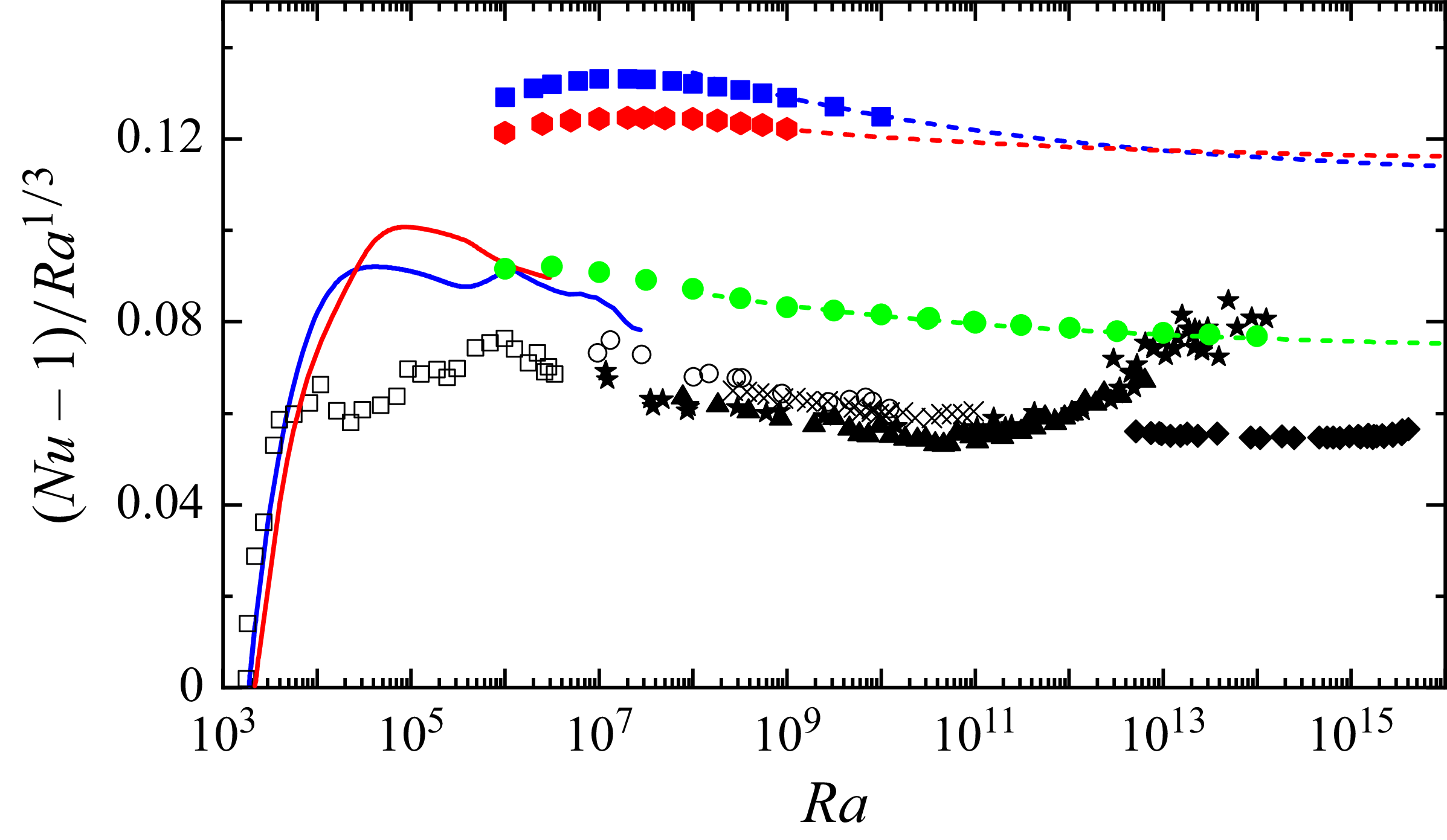
In figure 6, we present our results in the same format as figure 5 of Wen et al. (Reference Wen, Goluskin and Doering2022). Extending the 3-D ECS results to higher Rayleigh numbers is a computationally demanding task (recall that at each point we maximise $\textit{Nu}$
as shown in figure 2
a). Therefore, we rely on the theoretically predictable asymptotic behaviour of these states in the large-Rayleigh-number limit. The Nusselt number of the optimised solutions admits an expansion of the form
$\textit{Nu}$
as shown in figure 2
a). Therefore, we rely on the theoretically predictable asymptotic behaviour of these states in the large-Rayleigh-number limit. The Nusselt number of the optimised solutions admits an expansion of the form
 \begin{align} \textit{Nu}-1=Ra^{1/3} \big(C_0+C_1\! Ra^{-1/9}+O \big(Ra^{-2/9}\big)\big). \end{align}
This result directly follows from the asymptotic theory in § 3, where the intrinsic perturbation parameter is $O(Ra^{-1/9})$
. Note that the expansion (4.1) applies also to the 2-D roll cells, as the theory derived in § 3 shares the same asymptotic structure as that of Deguchi (Reference Deguchi2023). In theory, the coefficient
$O(Ra^{-1/9})$
. Note that the expansion (4.1) applies also to the 2-D roll cells, as the theory derived in § 3 shares the same asymptotic structure as that of Deguchi (Reference Deguchi2023). In theory, the coefficient $C_0$
is determined from the leading-order problem,
$C_0$
is determined from the leading-order problem, $C_1$
from the next-order problem and so on. However, although the leading-order equations (see (3.2), (3.4), (3.7)) were derived in § 3, solving them numerically is challenging. Therefore, here, we instead estimate the coefficients from the behaviour of the ECS. Since the ECS exhibit sufficiently good asymptotic behaviour around
$C_1$
from the next-order problem and so on. However, although the leading-order equations (see (3.2), (3.4), (3.7)) were derived in § 3, solving them numerically is challenging. Therefore, here, we instead estimate the coefficients from the behaviour of the ECS. Since the ECS exhibit sufficiently good asymptotic behaviour around $Ra = O(10^9)$
, we use two data points near this value to estimate
$Ra = O(10^9)$
, we use two data points near this value to estimate $C_0$
and
$C_0$
and $C_1$
in the truncated asymptotic prediction
$C_1$
in the truncated asymptotic prediction $\textit{Nu}-1=Ra^{1/3}(C_0+C_1\! Ra^{-1/9})$
:
$\textit{Nu}-1=Ra^{1/3}(C_0+C_1\! Ra^{-1/9})$
: $Ra = 10^9$
and
$Ra = 10^9$
and $10^{9.5}$
for the roll-cell and square cases, and
$10^{9.5}$
for the roll-cell and square cases, and $Ra = 10^{8.5}$
and
$Ra = 10^{8.5}$
and $10^{9}$
for the hexagon.
$10^{9}$
for the hexagon.
Nusselt number increment from the conducting state, compensated by $Ra^{1/3}$
. The data are the same as in figure 1, with the addition of extra experimental data. Triangle: Roche et al. (Reference Roche, Gauthier, Kaiser and Salort2020) (referred to as Grenoble
$Ra^{1/3}$
. The data are the same as in figure 1, with the addition of extra experimental data. Triangle: Roche et al. (Reference Roche, Gauthier, Kaiser and Salort2020) (referred to as Grenoble $\varGamma =1.14, \textit{Pr}\gt 1$
in Roche (Reference Roche2020) and Lohse & Shishkina (Reference Lohse and Shishkina2024)). Diamond: He, Bodenschatz & Ahlers (Reference He, Bodenschatz and Ahlers2022) (
$\varGamma =1.14, \textit{Pr}\gt 1$
in Roche (Reference Roche2020) and Lohse & Shishkina (Reference Lohse and Shishkina2024)). Diamond: He, Bodenschatz & Ahlers (Reference He, Bodenschatz and Ahlers2022) ( $\varGamma =1/3, \textit{Pr}\approx 0.8$
in Lohse & Shishkina (Reference Lohse and Shishkina2024)). Star: Chavanne et al. (Reference Chavanne, Chilla, Chabaud, Castaing and Hebral2001) (Grenoble
$\varGamma =1/3, \textit{Pr}\approx 0.8$
in Lohse & Shishkina (Reference Lohse and Shishkina2024)). Star: Chavanne et al. (Reference Chavanne, Chilla, Chabaud, Castaing and Hebral2001) (Grenoble $\varGamma =0.5$
,
$\varGamma =0.5$
, $\textit{Pr}\in (0.6,7)$
in Roche (Reference Roche2020)). The dashed lines are the fitting curves for squares (
$\textit{Pr}\in (0.6,7)$
in Roche (Reference Roche2020)). The dashed lines are the fitting curves for squares ( $0.111 +0.182Ra^{-1/9}$
), hexagons (
$0.111 +0.182Ra^{-1/9}$
), hexagons ( $0.115 +0.0706Ra^{-1/9}$
) and roll cells (
$0.115 +0.0706Ra^{-1/9}$
) and roll cells ( $0.0736 +0.100Ra^{-1/9}$
).
$0.0736 +0.100Ra^{-1/9}$
).

The green dashed line in figure 6 shows the asymptotic prediction for the 2-D roll-cell results. The curve accurately reproduces the computational results of Wen et al. (Reference Wen, Goluskin and Doering2022) even at $Ra=10^{14}$
. In the asymptotic limit, all higher-order correction terms vanish, and the classical scaling is recovered. Wen et al. (Reference Wen, Goluskin and Doering2022) showed that the optimised roll-cell solutions exhibit Nusselt numbers higher than those of DNS and experimental data around
$Ra=10^{14}$
. In the asymptotic limit, all higher-order correction terms vanish, and the classical scaling is recovered. Wen et al. (Reference Wen, Goluskin and Doering2022) showed that the optimised roll-cell solutions exhibit Nusselt numbers higher than those of DNS and experimental data around $\textit{Pr}=1$
. Note that the results by Chavanne et al. (Reference Chavanne, Chilla, Chabaud, Castaing and Hebral2001) in figure 6 appear to exceed the roll-cell result because we included data over a wider Prandtl number range than Wen et al. (Reference Wen, Goluskin and Doering2022).
$\textit{Pr}=1$
. Note that the results by Chavanne et al. (Reference Chavanne, Chilla, Chabaud, Castaing and Hebral2001) in figure 6 appear to exceed the roll-cell result because we included data over a wider Prandtl number range than Wen et al. (Reference Wen, Goluskin and Doering2022).
The blue and red dashed lines in figure 6 show the results for square and hexagon, respectively. The former asymptotic prediction performs well up to at least $Ra=10^{10}$
. Based on the roll-cell results, we expect the prediction to also agree with 3-D ECS numerical computations at higher Rayleigh numbers. Interestingly, the 3-D ECS results attain significantly higher Nusselt numbers than those of 2-D roll cells, as well as all experimental and DNS data reviewed in Lohse & Shishkina (Reference Lohse and Shishkina2024). Our results update
$Ra=10^{10}$
. Based on the roll-cell results, we expect the prediction to also agree with 3-D ECS numerical computations at higher Rayleigh numbers. Interestingly, the 3-D ECS results attain significantly higher Nusselt numbers than those of 2-D roll cells, as well as all experimental and DNS data reviewed in Lohse & Shishkina (Reference Lohse and Shishkina2024). Our results update $\aleph _{\textit{LB}}$
; this value is so large that experimental Nusselt numbers may not surpass it within the
$\aleph _{\textit{LB}}$
; this value is so large that experimental Nusselt numbers may not surpass it within the $ \textit{Ra} $
range shown in the figure, even when optimising the aspect ratio
$ \textit{Ra} $
range shown in the figure, even when optimising the aspect ratio $\varGamma$
and Prandtl number
$\varGamma$
and Prandtl number $\textit{Pr}$
. No matter how the upper bound theory is refined, the resulting
$\textit{Pr}$
. No matter how the upper bound theory is refined, the resulting $\aleph _{\textit{UB}}$
cannot fall below our
$\aleph _{\textit{UB}}$
cannot fall below our $\aleph _{\textit{LB}}$
.
$\aleph _{\textit{LB}}$
.
Note that, since our ECS computations are based on maximising $\textit{Nu}$
, discrepancies with experimental data in figure 6 are not unexpected. Although it is possible to artificially tune
$\textit{Nu}$
, discrepancies with experimental data in figure 6 are not unexpected. Although it is possible to artificially tune $L$
to match the ECS to experimental Nusselt numbers, we deliberately avoid doing so, as turbulence is unlikely to be governed by such a simple principle. The ECS possess only a small number of unstable eigenvalues and can, in principle, persist for relatively long periods within DNS. This makes our finding intriguing from the perspective of heat transport control. A possible direction for future work is to explore whether wall conditions can be engineered to stabilise such states, potentially enhancing heat transport by nearly a factor of two in certain cases.
$L$
to match the ECS to experimental Nusselt numbers, we deliberately avoid doing so, as turbulence is unlikely to be governed by such a simple principle. The ECS possess only a small number of unstable eigenvalues and can, in principle, persist for relatively long periods within DNS. This makes our finding intriguing from the perspective of heat transport control. A possible direction for future work is to explore whether wall conditions can be engineered to stabilise such states, potentially enhancing heat transport by nearly a factor of two in certain cases.
As already noted, our $\aleph _{\textit{LB}}$
exhibits classical scaling, so many researchers in the convection community would anticipate that turbulence in the ultimate regime will eventually push experimental data beyond
$\aleph _{\textit{LB}}$
exhibits classical scaling, so many researchers in the convection community would anticipate that turbulence in the ultimate regime will eventually push experimental data beyond $\aleph _{\textit{LB}}$
at sufficiently high
$\aleph _{\textit{LB}}$
at sufficiently high $ \textit{Ra} $
. However, demonstrating it remains an extremely challenging task and would represent a milestone for future convection experiments. This manifestation of what might be called ultimate-regime supremacy could, in principle, also be demonstrated by identifying corresponding ECS. Finding such ECS is far from straightforward, as our preliminary calculations suggest that the 3-D steady solutions bifurcating from the linear critical point all exhibit a similar trend in
$ \textit{Ra} $
. However, demonstrating it remains an extremely challenging task and would represent a milestone for future convection experiments. This manifestation of what might be called ultimate-regime supremacy could, in principle, also be demonstrated by identifying corresponding ECS. Finding such ECS is far from straightforward, as our preliminary calculations suggest that the 3-D steady solutions bifurcating from the linear critical point all exhibit a similar trend in $\textit{Nu}$
variation. The ECS that are disconnected from the laminar solution, analogous to those found in shear flows (Nagata Reference Nagata1990; Clever & Busse Reference Clever and Busse1992; Kawahara & Kida Reference Kawahara and Kida2001), cannot be excluded on theoretical grounds, although they lie beyond the scope of the present study.
$\textit{Nu}$
variation. The ECS that are disconnected from the laminar solution, analogous to those found in shear flows (Nagata Reference Nagata1990; Clever & Busse Reference Clever and Busse1992; Kawahara & Kida Reference Kawahara and Kida2001), cannot be excluded on theoretical grounds, although they lie beyond the scope of the present study.
Finally, we emphasise that the asymptotic theory developed here has the potential to be extended to unsteady, multi-scale states. Given that certain ECS are known to underpin chaotic states in shear flows (Kawahara, Uhlmann & Van Veen Reference Kawahara, Uhlmann and Van Veen2012; Wang et al. Reference Wang, Ayats, Deguchi, Meseguer and Mellibovsky2025), the scaling of our ECS may have some relevance to the classical regime of natural convection. The 3-D ECS computed by Motoki et al. (Reference Motoki, Kawahara and Shimizu2021) in a fixed domain exhibit multi-scale flow structures and could be considered better representatives of turbulence. However, to date, no multi-scale solutions have been extended to very high $ \textit{Ra} $
, and it remains unclear whether a corresponding asymptotic theory can be developed.
$ \textit{Ra} $
, and it remains unclear whether a corresponding asymptotic theory can be developed.
Acknowledgements
This research was supported by the Australian Research Council Discovery Projects (DP220103439 $\boldsymbol{\cdot}$
DP230102188), the Japanese Society for Promotion of Science (JSPS) KAKENHI (22H01401
$\boldsymbol{\cdot}$
DP230102188), the Japanese Society for Promotion of Science (JSPS) KAKENHI (22H01401 $\boldsymbol{\cdot}$
23K22672) and the Japan Science and Technology Agency (JST), PRESTO (JPMJPR23OC). The authors thank Professor D. Lohse for his helpful comments.
$\boldsymbol{\cdot}$
23K22672) and the Japan Science and Technology Agency (JST), PRESTO (JPMJPR23OC). The authors thank Professor D. Lohse for his helpful comments.
Declaration of interests
The authors report no conflict of interest.


 Open access