





1. Background
1.1. Steady streaming
The ability of zero-mean harmonic oscillations with frequency  $\hat {\omega }$ and wavenumber $\hat {k}$ to induce a mean flow via nonlinear advection is often referred to as steady streaming. This streaming can occur in the presence or absence of a background mean flow, and generally manifests itself in the vicinity of a solid boundary. The nature of the streaming can be characterized by the phase speed of the perturbation, $\hat {c} = \hat {\omega }/\hat {k}$. Temporal waves represent the limit of infinite phase speed, $\hat {k} \to 0$ and $\hat {c} \to \infty$, whereas spatial waves represent the zero phase speed limit, $\hat {\omega } \to 0$ and $\hat {c} \to 0$. Early studies on streaming focused largely on the temporal wave limit, in the absence of any background flow, in which case a net flow is induced by advection within a thin layer of fluid near the wall, known as the Stokes layer. For a fluid with kinematic viscosity $\hat {\nu }$, the Stokes layer is characterized by the length scale $\hat {\varDelta } = \sqrt {\hat {\nu }/\hat {\omega }}$. The advection that produces the net flow can be conceived as the result of a Reynolds stress, in which the average nonlinear interaction of velocity fluctuations results in a net transport. For a modern review, see Riley (Reference Riley2001) and the book-length treatment in Telionis (Reference Telionis1981).
While classical streaming analysis initially concentrated on situations with no mean background flow, this focus eventually shifted to steady streaming in the presence a background flow in the form of the canonical laminar boundary layer with mean free-stream velocity  $\hat {U}$ and characteristic length scale $\hat {\ell }$. In this case, in addition to the temporal and spatial waves described above, the intermediate travelling wave perturbations can be classified as either subcritical, with phase speed greater than the free-stream velocity, $|\hat {c}/\hat {U}| > 1$, or critical, with phase speed less than the free-stream velocity, $|\hat {c}/\hat {U}| < 1$.
Choi, Sreedhar & Stern (Reference Choi, Sreedhar and Stern1996) reported asymptotic and numerical solutions for the forced boundary layer equations with free-stream perturbations involving temporal, spatial and travelling waves, and noted significant differences among the three types of perturbations. Temporal perturbations produced a relatively small magnitude of streaming and a simple modification to the mean velocity profile that was captured well by asymptotic techniques. Previously, Lighthill (Reference Lighthill1954) proposed an asymptotic solution of the unsteady momentum equations in the limit of small temporal perturbation amplitudes,  $\varepsilon$, measured relative to the free stream. He closed the system of leading- and second-order momentum equations using the Kármán–Pohlhausen representation of the mean velocity profile and obtained solutions for the streaming in the limit of small and large Strouhal numbers, $St \equiv \hat {\omega } \hat {\ell }/\hat {U}$. The profile of velocity fluctuations near the wall exhibited an overshoot in amplitude, above the amplitude of the forcing, and a minimum in phase with respect to the free stream at a wall-normal location $\hat {y}_s \approx 4 \sqrt {2} \hat {\varDelta }$, which was originally reported by Richardson & Tyler (Reference Richardson and Tyler1929) and often called ‘Richardson's annular effect’. Later, Creff, Andre & Batina (Reference Creff, Andre and Batina1985) noted that the overshoot can appear in developing flows also, and was particularly strong in the developing region of a duct. The velocity overshoot is a consequence of the phase mismatch between the pressure force acting at the wall and momentum fluctuations of the fluid that have diffused some small distance away from the wall, resulting in an in-phase acceleration of the fluid (see the discussion in Panton (Reference Panton2013) and more detailed analysis below in § 3).
However, Choi et al. (Reference Choi, Sreedhar and Stern1996) noted that the streaming behaviour for spatial and travelling waves was significantly more complex than the case of temporal forcing. Spatial waves were observed to produce a significantly stronger streaming response, such that the streaming could no longer be considered a small perturbation to a base flow, and thus asymptotic methods were insufficient to describe the resulting flow field. And, as expected, travelling waves bridged the two extremes; they behaved similarly to temporal waves in the limit of high phase speeds, and showed the complex behaviour of spatial waves at lower phase speeds. This complex low-phase-speed behaviour was also noted by Hoepffner & Fukagata (Reference Hoepffner and Fukagata2009) and Mamori, Fukagata & Hoepffner (Reference Mamori, Fukagata and Hoepffner2010) in computations of a forced channel flow with travelling wave, suction and blowing at the wall. They reported significant modifications to the mean drag for perturbations with non-dimensional phase speeds  $0 < \hat {c}/\hat {U} < 1$ – in other words, for perturbations whose phase speeds matched the local mean velocity of the base flow. This special range of phase speeds results in the generation of a critical layer, a phenomenon not widely discussed in the classical streaming literature but fundamental to the problem of transition to turbulence.
1.2. Critical layers and transition
Similar to studies on streaming, transition studies also focus on the introduction of a small unsteady perturbation to a base laminar flow. In streaming research, the key challenge is to estimate the streaming velocity and its implications for skin friction and heat transfer, whereas in transition studies, the emphasis is on the shape and growth rate of the fluctuating velocity modes induced in the flow. When an infinitesimal travelling wave perturbation is applied to a laminar shear flow, the wall-normal location  $\hat {y}_c$, where the phase speed of the perturbation matches the local mean velocity $\hat {c} = \hat {u}(\hat {y} = \hat {y}_c)$, exhibits a singularity under a linearized inviscid stability analysis using the Rayleigh equation. The singularity at this critical point is ultimately resolved by the action of viscosity in a thin layer about the singularity, called the critical layer, as described by the viscous Orr–Sommerfeld equation. The consequence of the singularity is that low-phase-speed perturbations excite velocity modes within the flow that exhibit a prominent amplitude peak within the viscous critical layer along with a distinctive ${\rm \pi}$ phase jump far from the wall.
The use of travelling wave forcing can therefore produce two separate viscous regions in wall-bounded flows: the Stokes layer, characteristic of any temporal oscillations, and the critical layer, resulting from the travelling wave singularity (described in more detail in Godreche & Manneville (Reference Godreche and Manneville1998), § 2.7.4). Whether the critical layer is distinct or overlapping with the Stokes layer depends on the location of the critical layer and the relative thickness of the critical and Stokes layers. For infinitesimally small disturbances, asymptotic analysis can be applied to the linear Orr–Sommerfeld equation to obtain scalings for each of the layer thicknesses in terms of the small parameter  $(\hat {k} \hat {\ell } \, Re)$, where the Reynolds number is defined as $Re \equiv \hat {U} \hat {\ell }/\hat {\nu }$. In addition, Lin (Reference Lin1946) and Reid (Reference Reid1965) obtained an asymptotic approximation for the location of the critical point itself. However, these asymptotic results were developed assuming that the perturbations were vanishingly small and that the flows were quasi-parallel and thus do not capture the variation of the critical and Stokes layer length scales with streamwise extent or the case of nonlinear perturbations. Smith & Bodonyi (Reference Smith and Bodonyi1980) reported the critical layer length scale for different regions within a developing channel flow, avoiding the quasi-parallel assumption. And Haberman (Reference Haberman1972) and Bodonyi, Smith & Gajjar (Reference Bodonyi, Smith and Gajjar1983) both reported results for nonlinear critical layers, in which the critical layer location varies with perturbation amplitude, $\varepsilon$, and Reynolds number, $Re$, without direct dependence on the wavenumber.
1.3. Boundary layer streaming experiments and calculations
Efforts to measure experimentally streaming in the laminar boundary layer have been exceedingly rare across all forms of unsteady perturbations. Hill & Stenning (Reference Hill and Stenning1960) performed experiments on temporal wave disturbances and observed a strong correspondence with the theoretical streaming predictions of Lighthill (Reference Lighthill1954) and Nickerson (Reference Nickerson1957), at least for high and low Strouhal numbers, but weak correspondence at intermediate oscillatory frequencies. The primary travelling wave experiments were performed by Patel (Reference Patel1975), in which an oscillating flap in an open loop wind tunnel was used to introduce downstream-travelling free-stream velocity oscillations above a flat plate. The free-stream velocity  $\hat {U}$ was fixed at 10 m s $^{-1}$, and flap oscillation frequencies varied from $1$ to $10$ Hz, with the amplitude of velocity fluctuations reaching up to 10 % of the free stream. The phase speed of the travelling wave, $\hat {c}/\hat {U}$, was estimated to be $0.77$. Patel (Reference Patel1975) also extended the theory of Lighthill (Reference Lighthill1954) to finite wave speeds in order to reproduce the experimental amplitude and phase profiles of the fluctuating velocity modes measured across the laminar boundary layer. However, significant differences were observed between those experiments and the modified asymptotic theory.
Numerical techniques were also applied to achieve better matching to the travelling wave streaming experiments. Much earlier, Lin (Reference Lin1957) had developed a semi-analytical procedure to calculate the streaming velocity in the boundary layer by separating the instantaneous flow into mean and fluctuating contributions via the Reynolds decomposition. Although his approach was not adopted directly, Lam (Reference Lam1988) simplified the basic idea by assuming a fixed Blasius mean velocity profile and then integrating (by marching) an equation for the coupled velocity fluctuations. The incoming fluctuations were initialized by means of a series solution of the fluctuating equation about the leading edge of the plate. The resulting disturbance profiles showed much better agreement with the experiments of Patel (Reference Patel1975) than asymptotic approaches. But because the mean velocity profile was assumed fixed, this numerical approach was not able to resolve the streaming behaviour or the effect of the perturbations on the mean skin friction. Moreover, the experimental characterization of the disturbances used in Patel (Reference Patel1975) was subsequently re-examined by Ishaq & Bernstein (Reference Ishaq and Bernstein1987), who noted technical issues with the accuracy of the reported phase speeds, making exact theoretical comparisons difficult. Choi et al. (Reference Choi, Sreedhar and Stern1996) used both boundary layer and full Navier–Stokes numerical solutions, and also reported difficulty matching the experiments of Patel (Reference Patel1975).
The travelling wave experiments emphasized the fluctuating velocity mode shapes and focused only on Stokes layer behaviour, without addressing the effect of critical layers at all. In fact, experimental work related to laminar critical layers is confined largely to the transition literature. The effect of critical layer forcing was first studied by Schubauer & Skramstad (Reference Schubauer and Skramstad1947), who disturbed a laminar boundary layer with an oscillating wire, thereby introducing a travelling wave disturbance with an effective wave speed  $\hat {c}/\hat {U} \approx 0.35$. The velocity modes measured from this disturbance fit the predictions of an asymptotic solution of the Orr–Sommerfeld equation performed earlier by Schlichting (Reference Schlichting1950). Of course, in the context of transition, the effect of streaming was neglected and the base profile was assumed undisturbed. More recent studies regarding travelling wave wall forcing by Hoepffner & Fukagata (Reference Hoepffner and Fukagata2009) and Mamori et al. (Reference Mamori, Fukagata and Hoepffner2010) noted significant differences between systems with critical and subcritical disturbances, although these observations were confined to fully developed channel flows. The question of the practical consequences of critical layers on streaming in developing flows remains unexplored.
1.4. Approach
The presence of the two viscous layers – critical and Stokes – is key to understanding the increased complexity in travelling wave streaming behaviour in developing flows like the boundary layer. However, the interaction between these different layers as they evolve spatially, and the practical consequences of that interaction, are not well understood.
In § 2, we outline the forced unsteady boundary layer system and its numerical solution by extending the procedure of Lin (Reference Lin1957), and provide validation against the limited experiments and numerical simulations done previously. In § 3, we explain the streaming behaviour for the subcritical Stokes layer case for both upstream and downstream-travelling waves, and in § 3.1 we show how the sign of the streaming depends on the shape of the induced velocity modes. We then explore how the mode shapes change for the downstream-travelling critical layer case in §§ 3.2 and 3.3. In § 3.4, we show how the proximity of the two viscous layers is the primary determinant in the shape of the modes and thus the sign of the induced streaming. We report the effect of the localized variation in streaming on the skin friction in § 3.5, and finally we examine the dependence of the skin friction on the forcing strength, as described in § 3.6.
2. Forced laminar boundary layer model
A finite-amplitude travelling wave disturbance was introduced to the free stream above an otherwise zero-pressure-gradient flat-plate laminar boundary layer. Prandtl's boundary layer equation was used to model the laminar flow in order to reduce the computational complexity of the problem. However, due to the free-stream oscillatory motion, stricter Reynolds number assumptions were applied in order to assure the applicability of the boundary layer assumption, as discussed in Telionis (Reference Telionis1981) and below. The boundary layer equation was then decomposed using a Reynolds decomposition, and the mean and fluctuating velocity fields were solved numerically, in order to obtain the resulting changes in the mean velocity profile due to the travelling wave disturbances.
2.1. Forced boundary layer scaling
The free-stream velocity  $\hat {u}_{\infty }(\hat {x},\hat {t})$ was assumed to be the result of a steady contribution, $\hat {U}$, perturbed by a streamwise travelling wave disturbance, $u_1$, of the general form
 \begin{equation} \hat{u}_\infty(\hat{x},\hat{t}) = \hat{U}(1+\varepsilon u_1), \end{equation}
where  $\hat {U}$ is assumed constant and $u_1 = u_1[\hat {k} (\hat {x} - \hat {c} \hat {t})]$ is a dimensionless travelling wave moving downstream for $\hat {c} > 0$ and upstream for $\hat {c} < 0$. The hat, $\widehat {(\cdot )}$, denotes dimensional variables in the streamwise/wall-normal coordinates, $(\hat {x},\hat {y})$. The wavelength of the disturbance, $\hat {\lambda } = 2{\rm \pi} /\hat {k}$, was assumed greater than the boundary layer thickness, $\hat {\delta }_{99}$.
Following Telionis (Reference Telionis1981), the streamwise length scale of the oscillatory motion,  $\hat {\ell }_1 = |\hat {U}/\hat {\omega }|$, was used to define an oscillatory Reynolds number $Re_1 = \hat {U} \hat {\ell }_1/\hat {\nu }$, which was also assumed large, $Re_1 \gg 1$. $Re_1$ represents the time scale of the advection of the oscillating perturbation, whose characteristic velocity is the local mean velocity within the boundary layer, here approximated by the free-stream velocity $\hat {U}$. The Strouhal number, $St = \hat {\omega } \hat {\ell }/\hat {U}$, is related to the two Reynolds numbers by $Re = St\, Re_1$. The vertical (diffusive), oscillatory length scale of the Stokes layer, $\hat {\varDelta }$, is also related to the two Reynolds numbers by
 \begin{equation} \hat{\varDelta}/\hat{\ell} = St^{{-}1/2} Re^{{-}1/2}= Re^{{-}1} Re_1^{1/2}. \end{equation}
Although this scale is typically used only for temporal perturbations, it also describes the Stokes layer associated with travelling waves sufficiently far downstream from the leading edge, as discussed below in § 3.4.
The instantaneous velocity field  $(\hat {u},\hat {v})$ was non-dimensionalized according to $(u,v) = (\hat {u},\hat {v})/\hat {U}$. The coordinates were non-dimensionalized as $(x,y,t) = (\hat {x}/\hat {\ell }, \hat {y}/\hat {\ell },\hat {t} \hat {\omega })$, and the pressure was non-dimensionalized as $p = \hat {p}/\hat {\rho } \hat {U}^2$ where $\hat {\rho }$ is the fluid density, assumed constant.
In order to rewrite the instantaneous momentum equation in parameter-free form, with all the parameters expressed within only the perturbation velocity waveform,  $u_1$, we adopt the inertial stretching $(u,v,X,Y,T) = (u,v,x\,Re,y\,Re,t\,Re/St)$, which differs from the traditional coordinate stretching used in previous studies by e.g. Telionis & Romaniuk (Reference Telionis and Romaniuk1978). Capital letters here represent stretched coordinates. This choice of coordinates results in a perturbation velocity of the form $u_1 = u_1[ |c\, Re_1|^{-1} ({X} - c {T})]$, and a free-stream velocity
 \begin{equation} u_\infty(X,T) = 1 + \varepsilon u_1\left[|c\, Re_1|^{{-}1}\left(X - c T \right)\right], \end{equation}
where  $\varepsilon$, $Re_1$ and $c$ are domain-independent and constitute the three fundamental parameters of the system. The quantity $|c\, Re_1|$ represents the wavelength for the perturbation and is assumed large compared to the scale of $X$-variations of quantities within the boundary layer. In this formulation, the stretched coordinate $X$ is just the Reynolds number, $Re_x = \hat {U} \hat {x}/\hat {\nu }$, based on streamwise distance. Typically, $\hat {\ell }$ is taken as a characteristic length scale in the wall-normal direction, such as the boundary layer thickness $\hat {\delta }_{99}$ (or its asymptotic equivalents, the displacement thickness $\hat {\delta }^*$ or momentum thickness $\hat {\theta }$), in which case the Reynolds number $Re$ is related to $X$ by $Re \sim \sqrt {X}$ under the boundary layer assumptions.
2.2. Forced boundary layer equations
Employing the inertial scaling, the instantaneous boundary layer equations appear as
 \begin{equation} \frac{\partial u}{\partial T}+ u\,\frac{\partial u}{\partial X} + v\,\frac{\partial u}{\partial Y}={-}\frac{\partial p}{\partial X} + \frac{\partial^2 u}{\partial Y^2},\quad v(X,Y) ={-}\int_{0}^{Y} \frac{\partial}{\partial X} u(X,s)\,{\rm d} s, \end{equation}
where the wall-normal velocity  $v$ is defined through continuity, and the pressure gradient is defined through the free-stream dynamics,
 \begin{equation} \frac{\partial u_\infty}{\partial T}+ u_\infty\,\frac{\partial u_\infty}{\partial X} ={-}\frac{\partial p}{\partial X}, \end{equation}
and we assume that  ${\partial p}/{\partial Y}$ is negligible (based on the boundary layer approximation).
The time-averaging method of Lin (Reference Lin1957) was used to formulate an equation for the mean dynamics of the perturbed system by employing a Reynolds decomposition of the form  $q = \bar {q} + \tilde {q}$ to separate time-averaged contributions, denoted $\overline {(\cdot )}$, and temporal fluctuations, $\widetilde {(\cdot )}$. The fluctuating quantities are then stretched such that they appear as leading-order terms, with $q' = \tilde {q}/\varepsilon$.
Substituting the decomposition and re-scaling into (2.4a,b) and time-averaging yields
 \begin{align} \bar{u}\,\frac{\partial \bar{u} }{\partial X} + \bar{v}\,\frac{ \partial \bar{u} }{\partial Y} = \frac{\partial^2 \bar{u} }{\partial Y^2} + \varepsilon^2 \underbrace{\overline{\left({-}u'\,\frac{\partial u'}{\partial X} - v'\,\frac{ \partial u'}{\partial Y} \right)}}_{f(X,Y)},\quad \bar{v}(X,Y) ={-}\int_{0}^{Y} \frac{\partial}{\partial X} \bar{u}(X,s)\,{\rm d} s, \end{align}
where the sum of the two ‘Reynolds stress’ type terms is denoted  $f(X,Y)$ and represents the forcing to the mean dynamics from the fluctuations (also called the ‘apparent friction force’ in Schlichting & Gersten (Reference Schlichting and Gersten2000), § 5.3). The mean pressure gradient, ${\partial \bar {p}}/{\partial X}$, is zero for the flat-plate flow.
Subtracting the mean (2.6a,b) from instantaneous (2.4a,b) dynamics, and substituting the pressure gradient from (2.5), yields the fluctuating dynamics
 \begin{equation} \left.\begin{gathered} \frac{\partial u'}{\partial T}-\frac{\partial^2 u'}{\partial Y^2}- \frac{\partial u_1}{\partial T} = \left(\frac{\partial u_1}{\partial X} - \bar{u}\,\frac{\partial u'}{\partial X} - \bar{v}\, \frac{\partial u'}{\partial Y}\right)+ \left(- u'\,\frac{\partial \bar{u} }{\partial X} - v'\, \frac{\partial \bar{u} }{\partial Y}\right) \\ \quad{}+ \varepsilon \left\{ \left( u_1\,\frac{\partial u_1}{\partial X} - u'\, \frac{\partial u'}{\partial X} - v'\,\frac{\partial u'}{\partial Y}\right)- f(X,Y) \right\},\\ v'(X,Y) ={-}\int_{0}^{Y} \frac{\partial}{\partial X} u'(X,s) \, {\rm d} s. \end{gathered}\right\} \end{equation}
Note that in the free stream, the  $v'$ velocity component takes the form $v' = -Y ({\partial }/{\partial X}) \{ u_1[ |c\,Re_1|^{-1}(X - vT )] \}$ and thus is unbounded as $Y \to \infty$, due to the fact that the free-stream forcing is energetically unbounded, encompassing the entire domain. However, the forcing term $f(X,Y)$, along with all of the other terms in (2.6a,b), remains bounded. It is also important to note that (unlike ensemble-averaging) time-averaging and spatial differentiation/integration do not commute, due to the travelling wave form of the velocity forcing, thus the forcing cannot be easily expressed in the form of a Reynolds stress.
The streamwise mean dynamics (2.6a,b) depend on the dynamics of the streamwise fluctuations (2.7) via  $f(X,Y)$ and were solved, iteratively, subject to the following boundary conditions:
 \begin{equation} \left.\begin{gathered} (X,Y=0): \quad u'= v' = \bar{u} = \bar{v} = 0,\\ (X=0,Y): \quad u' = u_1({-}Re_1^{{-}1} T),\quad v' = 0,\quad \bar{u} = 1,\quad \bar{v} = 0,\\ (X,Y\to\infty): \quad \bar{u} = 1, \end{gathered}\right\} \end{equation}
which describe no-slip conditions at the wall for both mean and fluctuating quantities, followed by conditions for the uniform mean and temporal wave fluctuations at the inlet, with no wall-normal components. Finally, the free-stream matching condition was applied directly to the mean flow. The matching of the fluctuating streamwise velocity  $u'$ was satisfied automatically via the pressure forcing (2.5), which is uniform in the $Y$-direction under the boundary layer assumptions.
Utilizing a simple sine wave for the free-stream travelling wave perturbation,  $u_1 = \sin {(\cdots )}$, and substituting into (2.5), yields
 \begin{align} \varepsilon \frac{\left(1-c\right) }{|c \, Re_1|} \left\{ \sin{\left[\frac{\rm \pi}{2}- |c\,Re_1|^{{-}1}\left(X - c T \right)\right]} + \frac{\varepsilon/2}{(1-c)} \sin{\left[ 2|c\,Re_1|^{{-}1}\left(X - c T \right)\right]} \right\} ={-}\frac{\partial p}{\partial X}. \end{align}
Therefore, even though the velocity forcing (2.3) contains only the fundamental frequency  $Re_1^{-1}$, the pressure forcing (2.5) exhibits a $2Re_1^{-1}$ frequency component due to advection. The two non-dimensional forcing components are out of phase with each other by ${\rm \pi} /2$, and have amplitudes that differ by a factor of $({\varepsilon /2})/{(1-c)}$.
The  $2Re_1^{-1}$ forcing component is negligible on the assumption of low phase speed, i.e. $c\ll 1$, because ${\varepsilon }/{2(1-c)} \ll 1$. Therefore, many authors have followed the approach of Lighthill (Reference Lighthill1954) and simply Fourier-filtered the entire velocity field to eliminate this component altogether. However, Patel (Reference Patel1975) noted that if the second frequency is neglected, then as the phase speed approaches the mean free-stream velocity, $c \to 1$, there would be no actual pressure forcing in the problem at all, and the free-stream forcing would modify the boundary layer only via diffusion. Retaining the second frequency component is therefore necessary in the neighbourhood of phase speeds where $(1-c) \sim \varepsilon /2$. And in the limit $c \to 1$, this second frequency component becomes the dominant contribution to the (low-amplitude) forcing.
It is worth noting that even retaining the second forcing frequency throughout the boundary layer, as it reaches the outer edge of the boundary layer, the fluctuating velocity will exhibit only the fundamental frequency due to the advective terms in the streamwise momentum balance, and thus will satisfy (2.5) exactly.
2.3. Numerical approach
The mean momentum equation (2.6a,b) was solved in an iterative procedure, starting with an initialization scheme. First, (2.6a,b) was solved assuming  $f(X,Y) = 0$, to obtain an initial guess of the mean momentum balance. Then the mean momentum was used to solve the fluctuating dynamics (2.7) for $u'$ and $v'$, from which $f(X,Y)$ was calculated. The forcing, in turn, was substituted back into the mean dynamics (2.6a,b), to calculate an initial estimate of the mean momentum balance with all terms included. The mean flow variables $(\bar {u},\bar {v})$ were then substituted into the right-hand side of the fluctuating dynamics (2.7), to obtain an initial estimate of the fluctuating balance with all terms included, thus completing the initialization.
Once initialized, the fluctuating dynamics (2.7) were iterated in a prediction–correction procedure until a converged solution was found at each time step. The fluctuating dynamics were then marched forward in time, and the prediction–correction iteration was repeated at the new time step. The time-marching continued until a full period of the fundamental frequency was complete. The full period calculation was then repeated until convergence. The resulting converged period was then used to calculate  $f(X,Y)$ anew and update the mean momentum balance (2.6a,b). The updated mean momentum was fed into the fluctuating dynamics and iterated again, repeating the entire process until the mean balance converged. The calculation scheme is illustrated schematically in figure 1.
The iterative, predictor–corrector algorithm for the solution of the mean momentum balance (2.6a,b), using the fluctuating dynamics (2.7). Within the fluctuating dynamics, iterations are used to obtain convergence at each time step,  ${\rm \Delta} T$, and then over each full period, $2 {\rm \pi}\, Re_1$, before substituting and iterating within the mean momentum balance.

2.4. Finite differences and iteration
The system of equations (2.6a,b)–(2.9) was solved using finite differences on a rectangular domain that extended in the streamwise direction from  $X = 0$ to $X = 10^6$. The domain was sliced into eight streamwise segments due to memory constraints, and each segment was solved sequentially, where the exit conditions of each upstream segment were used as the inlet condition to the subsequent downstream segment. The domain in the wall-normal direction extended from $Y = 0$ to twice the downstream boundary layer thickness of each segment, $Y \approx 10 \sqrt {X}$.
The mean momentum balance (2.6a,b) was discretized using a second-order space-centred implicit finite difference scheme in the wall-normal direction, and a first-order backward scheme in the streamwise direction. This implicit finite difference formulation was solved using a fast and efficient tridiagonal matrix algorithm by Thomas (Reference Thomas1949). Mean quantities thus obtained were used as an input to the fluctuating flow equation (2.7), which was solved explicitly in a time-marching manner. As discussed before, an iterative prediction–correction approach was employed. At each iteration step, all input fluctuating derivatives were calculated using the previous step's prediction. Wall-normal derivatives of fluctuating quantities were calculated using a fourth-order space-centred scheme, whereas streamwise derivatives of fluctuating quantities were calculated using a second-order backward finite difference formulation to avoid dispersion errors. After a converged solution was obtained at a time step, the solution was marched forward to the next time step using a first-order scheme.
The mean and fluctuating momentum equations were iterated until a Euclidean norm convergence threshold between iterations of  $10^{-6}$ was satisfied, which is comparable to the approximation order, ${O}(X^{-1})$, of the neglected streamwise gradients in the momentum equation for the given domain size.
The grid resolution and time steps were designed to satisfy the grid convergence index (GCI) method of Roache (Reference Roache1994) to maintain small GCI values of approximately  $0.01$. The GCI variation with spatial resolution is described in Appendix A. This GCI criterion demanded a wall-normal discretization ${\rm \Delta} Y \sim {{0.067}} \sqrt {Re_1}$, a streamwise discretization ${\rm \Delta} X = 320$, and a temporal discretization ${\rm \Delta} T \sim 2{\rm \pi} \,Re_1 \times 10^{-4}$. The grid was defined conservatively to be uniform in each direction. Moreover, the Courant–Friedrichs–Lewy (CFL) number was verified to be below $0.5$ for stability.
The advantage of the Reynolds-decomposed technique of Lin (Reference Lin1957) over direct numerical solutions of the full momentum equations is apparent in the calculation times. All calculations were performed using matlab on a four-core desktop computer for a duration of approximately one day per  $X/10^6$. The mean skin friction coefficient was defined as $\bar {C}_f \equiv ({\partial \bar {u}}/{\partial Y})|_{Y=0}$. The uncertainty in $\bar {C}_f$, as estimated by dividing the convergence threshold (mentioned above) by the typical change in mean flow velocity near the wall, was obtained to be $0.3\,\%$.
2.5. Validity of boundary layer assumptions
The solutions are valid only where the appropriate boundary layer assumptions underlying the governing equations are satisfied. Telionis (Reference Telionis1981) noted that the steady Blasius regime requires  $X \gg 1$, while the oscillatory regime requires $X \gg \varepsilon ^{-2}$ and $Re_1 \gg \varepsilon ^{-2}$ such that the unsteady terms are not less significant than the neglected streamwise diffusion terms. The latter requirement is only marginally satisfied for the small $\varepsilon$ considered here, but can also be validated by direct comparison of the neglected streamwise diffusion of the mean flow, ${\partial ^2 \bar {u}}/{\partial X^2}$, to the wall-normal diffusion of the streaming itself, ${\partial ^2 \bar {u}_s}/{\partial Y^2}$, where the streaming velocity $\bar {u}_s$ is defined as the difference between the mean velocity profile $\bar {u}$ and the unforced laminar profile $\bar {u}_{0}$, as $\bar {u}_s = \bar {u} - \bar {u}_{0}$. The map of this comparison is shown in Appendix B and confirms that wherever measurable streaming was observed, the boundary layer approximation is satisfied in a self-consistent way.
The upper limit on  $X$, prior to transition, is taken as $X \approx 10^6$, following Schlichting & Gersten (Reference Schlichting and Gersten2000), although this is likely an overestimate due to the perturbed free stream. The applicability of the analysis to practical flows where transition may occur will be discussed in more detail in § 3.6.
All calculations were performed over a domain that extended from the leading edge to  $X = 10^6$, corresponding to a maximum downstream Reynolds number $Re_\theta = 660$ based on momentum thickness $\bar {\theta }$.
The numerical solutions were validated against experimental results for temporal disturbances reported by Hill & Stenning (Reference Hill and Stenning1960) and for travelling wave disturbances reported by Patel (Reference Patel1975), and were compared to the alternative numerical approaches of Lam (Reference Lam1988) and Choi et al. (Reference Choi, Sreedhar and Stern1996), as discussed below.
2.6. Validation
The flow calculations in the limit of very high phase speed,  $c^{-1} = 0.01$, were compared against temporal ( $c^{-1}=0$) perturbation experiments performed by Hill & Stenning (Reference Hill and Stenning1960). Figure 2(a) shows the amplitude and phase of the perturbations at matched frequency, amplitude and streamwise position.
Amplitude,  $|u'|$ (black, left axis), and phase, $\phi ^{(u)}$ (grey, right axis), of streamwise fluctuations as functions of wall-normal distance for: (a) comparison with temporal experiments by Hill & Stenning (Reference Hill and Stenning1960) at $(\varepsilon, Re_1, c^{-1}, X) = (0.1, 1.2\times 10^4, 0, 6 \times 10^4)$, shown in circles, versus the present calculation, with $c^{-1}=0.01$, shown in solid lines; (b) comparison with travelling wave experiments by Patel (Reference Patel1975) (circles) for $(\varepsilon, Re_1, c^{-1}, X) = (0.056, 2.2\times 10^5, 2, 1.4\times 10^5)$, and simulations by Choi et al. (Reference Choi, Sreedhar and Stern1996) (dashed lines) versus the present calculation (solid lines).

For the experimental reported phase speed  $c^{-1}= 1.3$, comparisons were performed against the experiments of Patel (Reference Patel1975) and the full Navier–Stokes numerical solutions of Choi et al. (Reference Choi, Sreedhar and Stern1996), as shown in figure 2(b). However, Choi et al. (Reference Choi, Sreedhar and Stern1996) used $c^{-1} = 2$ for better matching with the experimental results. In fact, there is some doubt about the precise wave speeds obtained in the experiments of Patel (Reference Patel1975), thus there is some arbitrariness involved in the matching. Lam (Reference Lam1988) and Evans (Reference Evans1989) cite private communications for believing that the correct $c^{-1}$ value corresponding to the experiments should be $1.65$. Figure 3 illustrates the effect of the choice of phase speed on the quality of the experimental match. The current calculations compare well with experiments and previous numerical solutions, within these experimental uncertainties.
Amplitude,  $|u'|$ (black, left axis), and phase, $\phi ^{(u)}$ (grey, right axis), of streamwise fluctuations as functions of wall-normal distance for (a) a comparison with travelling wave experiments by Patel (Reference Patel1975) (circles) and simulations by Lam (Reference Lam1988) (dashed lines) at $(\varepsilon, Re_1, c^{-1}, X) = (0.056, 8.8\times 10^4, 1.65, 1.4\times 10^5)$ versus the present calculation, shown in solid lines. (b) A change in $c^{-1}$ value to $1.7$ for the present calculations provides an even better amplitude matching.

It is important to note that the numerical approach of Lam (Reference Lam1988) assumed a fixed mean velocity profile and thus allowed for only one-way coupling between the mean flow and the perturbations, so his technique is not capable of predicting streaming. Also, by assuming a self-similar boundary layer profile even near the leading edge, Lam's approach does not allow for the simultaneous development of the boundary layer, Stokes layer and critical layers. It is difficult to assess the effects of these different assumptions on the resulting flow field. But because we sought to predict the streaming and not merely the fluctuating velocity mode profiles, we needed to adopt an approach that included explicitly two-way coupling between the fluctuations and the mean flow.
3. Results and discussion
3.1. Velocity modes and streaming
The time-averaged effect of the free-stream perturbation results in velocity streaming via the forcing term
 \begin{equation} f(X,Y) = \overline{\left({-}u'\,\frac{\partial u'}{\partial X} - v'\,\frac{ \partial u'}{\partial Y} \right)}, \end{equation}
which appears in the mean momentum balance in (2.6a,b). The sign of the forcing determines whether  $f$ serves as a source or sink of momentum across the boundary layer, and thus determines the behaviour of the streaming. The sign of $f$ depends on the time-averaged interaction between the streamwise, $u'$, and wall-normal, $v'$, modes and their gradients. Because the perturbation is a single-frequency harmonic, the sign of the time-averaged interaction will be controlled entirely by the phase difference between these interacting modes.
We will first determine the phases of the different modes that appear in the forcing, and describe them physically in terms of their spatial inclination. Then this information will be used to explain the net forcing and the streaming behaviour. Modes that are orthogonal, with phase lag  $\pm {\rm \pi}/2$, will produce no net contribution when averaged over a single period. Modes that are in phase, with phase lag $0$, or out of phase, with phase lag $\pm {\rm \pi}$, will result in positive or negative time-averaged contributions, respectively.
In order to describe the phase of the interacting modes, we write the real-valued modes  $u'$ and $v'$ in complex form, in terms of magnitudes, $|u'|$ and $|v'|$, and temporal phases, $\phi ^{(u)}$ and $\phi ^{(v)}$, as
 $$\begin{gather} u'(X,Y,T) = \text{Im}\left[ |u'|(X,Y) \exp\left({{\rm i} \left\{ |Re_1\, c|^{{-}1}\left[X - c \left(T + Re_1\,\phi^{(u)}(X,Y) \right)\right] \right\}}\right) \right], \end{gather}$$
 $$\begin{gather}v'(X,Y,T) = \text{Im}\left[ |v'|(X,Y) \exp\left({{\rm i} \left\{ |Re_1\, c|^{{-}1}\left[X - c \left(T + Re_1\,\phi^{(v)}(X,Y) \right)\right] \right\}}\right) \right], \end{gather}$$
where all phases are measured with respect to the phase of the free-stream perturbation, which is taken as  $\phi ^{(u)}(X,Y \to \infty ) = 0$, consistent with the definition of the perturbation in (2.3).
The two contributions to the forcing depend on the phase lags between  $u'$ and $u'_X$, and between $v'$ and $u'_Y$. From differentiation, the phase $\phi ^{(u_X)}$ of $u'_X$ is related to the phase $\phi ^{(u)}$ of $u'$ by
 \begin{equation} \phi^{(u_X)} = \phi^{(u)} - \text{sgn}(c)\, \text{arg}\left[|u'|^{{-}1}|u'|_X + {\rm i}\,|c\,Re_1|^{{-}1} - {\rm i}\, \text{sgn}(c)\,\phi^{(u)}_X \right], \end{equation}
where the sign of the phase speed  $c$ is denoted $\textrm {sgn}(c)$ and represents the direction of propagation of the perturbations. Because the wavelength of the perturbation is assumed long compared to the length scale of streamwise variations, i.e. $|c\,Re_1|^{-1} \ll |u'|^{-1}|u'|_X,\phi ^{(u)}_X$, the wavenumber term $|c\, Re_1|^{-1}$ is the dominant contribution, and the phase relation can be approximated as
 \begin{equation} \phi^{(u_X)} \approx \phi^{(u)} - \text{sgn}(c)\,\frac{\rm \pi}{2}. \end{equation}
Therefore, the  $u'$ and $u'_X$ modes are expected to be orthogonal to each other, resulting in negligible contribution to the forcing and thus the streaming. This is ultimately a consequence of the boundary layer assumptions regarding gradients in the $X$-direction. However, the remaining forcing term, involving $u'_Y$ and $v'$, is more complicated.
The phase  $\phi ^{(u_Y)}$ of $u'_Y$ is found by differentiation as
 \begin{equation} \phi^{(u_Y)} = \phi^{(u)} - \text{sgn}(c) \, \text{arg}[|u'|^{{-}1}|u'|_Y - {\rm i}\, \text{sgn}(c)\,\phi^{(u)}_Y ]. \end{equation}
Continuity is then used to relate the phases of  $u'$ and $v'$, employing the long wavelength approximation from above, as
 \begin{equation} \phi^{(v)} \approx \phi^{(u)} + \text{sgn}(c)\,\frac{\rm \pi}{2} + \text{sgn}(c) \arg{[|v'|^{{-}1}|v'|_Y -{\rm i}\,\text{sgn}(c)\,\phi_Y^{(v)}]}. \end{equation}
In both of these relations, the phase trends depend on the mode shapes. In particular, the spatial inclination of the  $u'$ mode is given by $-\textrm {sgn}(c)\,\phi _Y^{(u)}$. When $-\textrm {sgn}(c)\,\phi _Y^{(u)} < 0$, the mode is inclined in the downstream direction with respect to the wall, whereas when $-\textrm {sgn}(c)\,\phi _Y^{(u)} > 0$, the mode is inclined in the upstream direction. The inclination of the mode therefore determines the imaginary contribution to the phase argument. In the case where the mode experiences an extremum in amplitude, i.e. where $|u'|_Y$ changes sign, the argument will exhibit a phase jump of $\pm {\rm \pi}$, and the sense of the jump will be determined by the inclination of the mode.
Consider the case of the subcritical modes, in which the phase speed satisfies  $|c^{-1}| < 1$ so that no critical layer is generated. The $u'$ and $v'$ spatial mode shapes, over one wavelength, are shown in figure 4(a) for upstream-travelling subcritical waves, and in figure 4(b) for downstream-travelling subcritical waves. Starting at the wall, the amplitude of the fluctuations is zero, thus $|u'|,|v'| \to 0$, which means that we have the phase relations
 $$\begin{gather} \phi^{(u_Y)} = \phi^{(u)}, \end{gather}$$
 $$\begin{gather}\phi^{(v)} = \phi^{(u)} + \text{sgn}(c)\,\frac{\rm \pi}{2}, \end{gather}$$
so  $u'_Y$ and $v'$ are orthogonal at the wall and contribute nothing to the forcing. The corresponding temporal phase plots show that the $v'$ mode leads (lags) the $u'$ mode in time by ${\rm \pi} /2$ for downstream (upstream) travelling waves.
Subcritical ( $|c^{-1}|<1$) spatial modes of streamwise ( $u'$) and wall-normal ( $v'$) components of fluctuating velocity, and polar phase profiles of the velocity components and gradients of streamwise velocity ( $u'_Y$, $u'_X$). The grey line indicates the Stokes layer scale; the radial range of polar plots is same as the $Y$ range of adjacent contour plots. (a) The upstream-travelling wave with $(\varepsilon, Re_1, c^{-1}, X) = (0.01, 2\times 10^4, -0.4, 10^6)$ and downstream spatial $u'$ inclination. Here, the $v'$ and $u'_Y$ modes are in phase, resulting in a negative contribution to the forcing. (b) The downstream-travelling wave with $(\varepsilon, Re_1, c^{-1}, X) = (0.01, 2\times 10^4, +0.4, 10^6)$ and upstream spatial $u'$ inclination. Here, the $v'$ and $u'_Y$ modes are out of phase, resulting in a positive contribution to the forcing.

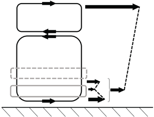
The continuity relation (3.9) allows us to describe, pictorially, a temporal cycle of a particle tracing the path of the modal oscillations, shown in figure 5. For an upstream-travelling wave, shown in figure 5(a), the  $v'$ mode lags the $u'$ mode, resulting in a clockwise path. For a downstream-travelling wave, shown in figure 5(b), the $v'$ mode leads the $u'$ mode, resulting in a counter-clockwise path. Hoepffner & Fukagata (Reference Hoepffner and Fukagata2009) used a similar heuristic to analyse the transport associated with travelling wave suction and blowing at a channel wall. They noted that in the absence of viscosity, the particle would make the circuit with perfect symmetry between upstream and downstream movements. However, viscosity near the wall causes an asymmetry in the particle motion, suppressing the particle motion near the wall compared to that far away from the wall. The viscous region, i.e. the Stokes layer, is denoted by a grey line.
An illustration of the path of a fluid particle of the perturbed flow, over one time period, in the notional absence of any mean flow. (a) The path, in solid black line, corresponding to the upstream-travelling subcritical mode shown in figure 4(a), which results in downstream mode inclination  $-\textrm {sgn}(c)\,\phi _Y^{(u)} < 0$. (b) The path corresponding to the downstream-travelling subcritical mode shown in figure 4(b), which results in upstream mode inclination $-\textrm {sgn}(c)\,\phi _Y^{(u)} > 0$. The viscous Stokes layer is illustrated by the grey line; the arrows indicate the relative particle displacements, taking into account the effect of viscosity; the dashed black line illustrates the resulting mode inclination.

For the upstream-travelling wave in figure 5(a), the backward velocity in the viscous Stokes layer near the wall will be suppressed more than the forward velocity far away from the wall, and this asymmetry will tend to tilt the mode in the outer region in the downstream direction with respect to the wall, thus  $-\textrm {sgn}(c)\,\phi _Y^{(u)} < 0$. For the downstream-travelling wave in figure 5(b), the forward velocity in the viscous Stokes layer near the wall will be suppressed more than the backward velocity far away from the wall, and this asymmetry will tend to tilt the mode in the outer region in the upstream direction with respect to the wall, thus $-\textrm {sgn}(c)\,\phi _Y^{(u)} > 0$.
The inclination inside the viscous near-wall region itself can also be analysed. For the downstream-travelling case in figure 5(b), very near the wall, there is a significant variation in the wall-normal velocity component, with zero velocity at the wall and increasing wall-normal flow farther away (assuming that the viscous effects are comparable). This means that a particle at a given  $Y$ location very near the wall will have a longer residence time at that height than a particle a bit farther away, which will be moving upwards faster. Therefore, within the viscous layer, we also expect an upstream inclination of modes, due to the effect of the gradient in $|v'|$. (The opposite is true for the case of wall suction and blowing studied by Hoepffner & Fukagata (Reference Hoepffner and Fukagata2009), where they observed a downstream inclination inside the viscous region near the wall, because the blowing is strongest at the wall and diffuses away from the wall, unlike the case of free-stream forcing considered here.)
Thus in both the outer and inner regions of the boundary layer, we expect an upstream inclination of the velocity modes for a downstream-travelling subcritical wave, and the opposite for the upstream-travelling subcritical wave. The mode inclination is visible most prominently for the  $u'$ modes in figure 4. The inclination information about the modes can then be used to determine the subsequent phase behaviour farther away from the wall.
Moving away from the wall, both upstream- and downstream-travelling waves exhibit a maximum amplitude in  $u'$ around the Stokes layer height, as shown in figure 4. The downstream-travelling wave in figure 4(b) also shows a relative minimum even farther from the wall due to the lower effective forcing at that phase speed. The extrema in the amplitude result in a phase jump in $u'_Y$ via the argument in (3.6) given by
 \begin{equation} -\text{sgn}(c)\,\text{arg}[|u'|^{{-}1}|u'|_Y - {\rm i}\, \text{sgn}(c)\,\phi^{(u)}_Y ]. \end{equation}
Moving away from the wall and crossing a relative amplitude maximum means that  $|u'|_Y$ shifts from positive to negative. For the upstream-travelling wave, $-\textrm {sgn}(c)\,\phi _Y^{(u)} < 0$, therefore (3.10) produces a phase jump $-{\rm \pi}$. This clockwise phase addition is illustrated by the black line in the polar phase plot in figure 4(a), representing the phase of $u'_Y$, which starts in phase with $u'$ at the wall and jumps by $-{\rm \pi}$ as it crosses the Stokes layer, marked in grey. The same is true for the downstream-travelling wave, where $-\textrm {sgn}(c)\,\phi _Y^{(u)} > 0$, and therefore (3.10) also produces a phase jump of $-{\rm \pi}$. However, the downstream-travelling wave exhibits a relative minimum in amplitude farther out, which results in a second jump of $-{\rm \pi}$, re-aligning the phase of $u'_Y$ with $u'$ far from the wall, as seen in the polar plot in figure 4(b).
Having described the phase variation of the  $u'_Y$ mode, we are left to describe the $v'$ modes in order to complete the picture of the forcing. However, the $v'$ modes are much simpler: the argument in (3.7) does not contribute any phase jumps because there are no extrema in the amplitude of $v'$ for the Stokes layer forced from the free stream. Therefore, the phase of $v'$ hovers about its initial wall value across the boundary layer
 \begin{equation} \phi^{(v)} \approx \phi^{(u)} + \text{sgn}(c)\,\frac{\rm \pi}{2}. \end{equation}
 With both phases described, we can consider the effect of the two modes on the time-averaged forcing. If the phase of  $v'$ is roughly constant across the boundary layer, leading or lagging $u'$ by ${\rm \pi} /2$, while the phase of $u'_Y$ jumps by $-{\rm \pi}$ with respect to the phase of $u'$, then the $v'$ and $u'_Y$ modes will necessarily be in or out of phase in some region of the boundary layer, resulting in a net contribution to the local time-averaged forcing. For the case of the upstream-travelling wave in figure 4(a), $v'$ and $u'_Y$ will be in phase, resulting in a negative forcing, from (3.1); whereas the modes in the downstream-travelling wave in figure 4(b) are out of phase, resulting in a positive forcing.
The effect of the localized forcing on the streaming profiles is shown in figure 6, where the streaming velocity  $\bar {u}_s$ was defined above as the difference between the mean velocity profile and the unforced laminar profile $\bar {u}_s = \bar {u} - \bar {u}_{0}$. As expected, when the modes are in phase, the dominant forcing is negative and the streaming is negative. For out-of-phase modes, the streaming is positive. Thus the sign of the streaming associated with the presence of a Stokes layer can be described entirely in terms of the shape and inclination of its velocity modes. The magnitude of the streaming of course depends on the relative magnitude of the $v'$ and $u'_Y$ modes, which are highest near the wall but are not easily described by the type of heuristic analysis employed here to capture the correct sign.
Streaming velocity profiles  $\bar {u}_s(Y)$ for the subcritical perturbations in figure 4. For the upstream-travelling wave in figure 4(a) with $(\varepsilon, Re_1, c^{-1}, X) = (0.01, 2\times 10^4, -0.4, 10^6)$, the modes are in phase with negative forcing and negative streaming, marked as a dotted line. For the downstream-travelling wave in figure 4(b) with $(\varepsilon, Re_1, c^{-1}, X) = (0.01, 2\times 10^4, +0.4, 10^6)$, the modes are out of phase with positive forcing and positive streaming, marked as a dash-dotted line.

3.2. Streaming with a critical layer
In the presence of a critical layer, the mode shapes change significantly thus the streaming is also modified. Classically, two-dimensional critical layers exhibit a viscous region about the critical point itself,  $Y_c$ (corresponding to $\hat {y}_c$, defined above in the unstretched coordinates), and also a phase jump in the $u'$ mode at the location of the maximum in the amplitude of the $v'$ modes, which is usually much farther from the wall than $Y_c$. This phase jump is associated with the pair of inviscid solutions to the critical layer problem described in Schlichting (Reference Schlichting1950). Therefore, in the case of the critical layer, we need to re-analyse the phase relationship between $v'$ and $u'_Y$, taking into account that $u'$ experiences a phase jump.
To simplify the analysis, the continuity formulation in (3.7) is substituted into (3.6) to obtain
 \begin{equation} \phi^{(u_Y)} = \overbrace{\phi^{(v)} - \frac{\rm \pi}{2} - \arg{\left[|v'|^{{-}1}|v'|_Y -{\rm i}\phi_Y^{(v)}\right]}}^{\phi^{(u)}} - \arg[|u'|^{{-}1}|u'|_Y - {\rm i}\phi^{(u)}_Y ], \end{equation}
where  $c^{-1}>1$ is necessary for the existence of a critical layer, which exists only in downstream-travelling waves. If we make the very strong simplifying assumption that the phase jump is sharp, such that $|u'|$ crosses zero, then we can neglect the argument associated with the $u'$ mode in the vicinity of the maximum amplitude in $v'$, to obtain
 \begin{equation} \phi^{(u_Y)} \approx \phi^{(v)} - \frac{\rm \pi}{2} - \text{arg}[|v'|^{{-}1}|v'|_Y - {\rm i}\phi^{(v)}_Y ]. \end{equation}
For the subcritical case described earlier by (3.6), the phase jump in  $u'_Y$ depended on the mode shape of $u'$; for the critical case described here in (3.13), the phase jump in $u'_Y$ depends on the mode shape of $v'$. Figure 7 shows the $u'$ and $v'$ spatial mode shapes for perturbations with a critical layer ( $c^{-1} = 4$) at two different streamwise locations. At the upstream location in figure 7(a), we note that $v'$ modes are inclined slightly downstream, whereas at the downstream location in figure 7(b), the $v'$ modes are inclined slightly upstream.
Critical ( $c^{-1}>1$) spatial modes of streamwise ( $u'$) and wall-normal ( $v'$) components of fluctuating velocity, and polar phase profiles of the velocity components and gradients of streamwise velocity ( $u'_Y$, $u'_X$). The grey line indicates the Stokes layer scale; the dashed black line indicates the critical point; and the radial range of the polar plots is the same as the $Y$ range of adjacent contour plots. (a) The downstream-travelling wave with $(\varepsilon, Re_1, c^{-1}, X) = (0.01, 2\times 10^4, +4, 10^5)$ and downstream spatial $v'$ inclination. Here, the $v'$ and $u'_Y$ modes are in phase, resulting in a negative contribution to the forcing. (b) The downstream-travelling wave with $(\varepsilon, Re_1, c^{-1}, X) = (0.01, 2\times 10^4, +4, 10^6)$ and (slightly) upstream spatial $v'$ inclination. Here, the $v'$ and $u'_Y$ modes are out of phase, resulting in a positive contribution to the forcing.

Because all critical modes are downstream-travelling, very near the wall they appear similar to the subcritical downstream mode shown in figure 4(b), where the  $v'$ mode leads the $u'$ mode, resulting in a counter-clockwise path. However, far from the wall, at the location of the maximum amplitude of $v'$, the $u'$ mode experiences a phase jump. The direction of the phase jump indicates whether the path at the top of the mode is also counter-clockwise or whether it switches direction to be clockwise.
Because the  $v'$ mode always has, at most, one relative maximum within the boundary layer, the phase jump in (3.13) depends ultimately only on the inclination of the $v'$ modes. If the modes are inclined upstream, then the argument produces a phase jump $-{\rm \pi}$; if the modes are inclined downstream, then the argument produces a phase jump $+{\rm \pi}$. And this inclination does indeed indicate the direction of the phase jump in $u'_Y$, as shown in the corresponding polar phase plots in figure 7, where the downstream-inclined $v'$ modes in figure 7(a) exhibit a phase jump $+{\rm \pi}$, and upstream-inclined $v'$ modes in figure 7(b) exhibit a $-{\rm \pi}$ phase jump.
Therefore, the different mode inclinations between the two streamwise positions for the critical perturbations are direct indications of the direction of the phase jump induced by the presence of the critical layer. Moreover, as with the Stokes layer, the direction of the phase jump determines whether the  $u'_Y$ and $v'$ modes are in phase or out of phase, and thus controls the sign of the forcing and the streaming.
At the wall, the  $u'_Y$ and $v'$ modes are orthogonal, with phase lag $-{\rm \pi} /2$, resulting in no contribution to the forcing. Therefore, if the $v'$ modes are inclined slightly downstream, as in figure 7(a), and the phase jump is $+{\rm \pi}$, then the $v'$ and $u'_Y$ modes will be in phase and the forcing will be negative; whereas if the $v'$ modes are inclined slightly upstream, as in figure 7(b), and the phase jump is $-{\rm \pi}$, then the $v'$ and $u'_Y$ modes will be out of phase and the forcing will be positive.
Recall that the subcritical downstream-travelling wave shown in figure 4(b) generated positive forcing, whereas the inclusion of the critical layer can produce either positive or negative forcing, depending on the mode inclination. The ability of the critical layer to reverse the forcing as compared to the subcritical case was also reported by Hoepffner & Fukagata (Reference Hoepffner and Fukagata2009) for the problem of travelling wave wall suction/blowing in a channel.
The effect of the localized forcing on the streaming profiles is shown in figure 8. The streaming associated with the presence of a critical layer can therefore be described entirely in terms of inclination of its wall-normal velocity velocity mode, which varies with streamwise extent. It remains to describe why the critical layer produces different wall-normal inclinations (or, equivalently, different phase jump directions) at different streamwise locations.
Streaming velocity profiles  $\bar {u}_s(Y)$ for the subcritical perturbations in figure 7. For figure 7(a), with $(\varepsilon, Re_1, c^{-1}, X) = (0.01, 2\times 10^4, +4, 10^5)$, the modes are in phase with negative forcing and negative streaming, marked as a dotted line. For figure 7(b), with $(\varepsilon, Re_1, c^{-1}, X) = (0.01, 2\times 10^4, +4, 10^6)$, the modes are out of phase with positive forcing and positive streaming, marked as a dash-dotted line.

3.3. Wall-normal mode inclination
The variation of the wall-normal mode inclination, measured at the location of the local maximum amplitude of  $v'$ within the boundary layer, with respect to streamwise location $X$ and inverse phase speed $c^{-1}$, is shown in figure 9(a). Very far upstream and at low $c^{-1}$, the $v'$ mode does not exhibit a local maximum within the boundary layer, thus no mode inclination is reported. There appears to be a distinct region, demarcated by the dashed line, in which the $v'$ modes are inclined upstream, $\phi _Y^{(u)} < 0$, surrounded by a larger region where the $v'$ modes are inclined downstream, $\phi _Y^{(u)} > 0$. The changing inclination appears to be due to a combination of the spatial development and strength of the critical and Stokes layers within the boundary layer.
(a) The gradient of the  $v'$ phase, $\phi _Y^{(v)}$, evaluated at the location where $|v'|$ is maximum. The black dashed line highlights where the change in inclination occurs. Grey indicates regions where no local maximum in $|v'|$ existed. (b) The ratio of critical point and Stokes layer heights, $Y_c/Y_s$, where the solid black line shows the intersection of the two layers as described in (3.17), for $(\varepsilon, Re_1) = (0.01, 2\times 10^4)$.

Figure 9(b) shows the ratio of the wall-normal locations of the critical and Stokes layer scales,  $Y_c/Y_s$, as a function of $X$ and $c^{-1}$, where the intersection of the two points is marked in a solid line. The region of downstream inclined $v'$ modes appears to correspond to a region where the critical and Stokes layers are located close to one another.
We can describe the inclination of the  $v'$ modes by a heuristic analysis of particle paths similar to that presented above, shown in figure 10. When the critical and Stokes layers coincide, as in figure 10(b), the viscous region is not significantly larger than in the subcritical downstream-travelling wave case, and the modes are inclined upstream following the heuristic argument outline in figure 5(b) for the very-near-wall region. However, when the critical and Stokes layers are distinct, as in figure 10(a), there are two separate viscous regions with a region between them where viscosity is less important. Within the first viscous region near the wall, the residence time argument due to the $v'$ amplitude yields an upstream inclination, as is true for all downstream-travelling waves. But in the gap between the two viscous layers, the lack of friction produces a downward inclination of the modes. This reversal in inclination from upstream to downstream between the Stokes and critical layers is visible very near the wall in figure 7(a).
An illustration of the path, in solid black line, of a fluid particle of the perturbed flow, over one time period, in the notional absence of any mean flow. (a) The path corresponding to the critical mode shown in figure 7(a), which results in downstream mode inclination,  $\phi _Y^{(u)} > 0$. (b) The path corresponding to the critical mode shown in figure 7(b), which results in upstream mode inclination, $\phi _Y^{(u)} < 0$. The viscous Stokes layer is illustrated by the solid grey line, the critical layer by the dashed grey line. The arrows indicate the relative particle displacements, taking into account the effect of viscosity; the dashed black line illustrates the resulting mode inclination. Note that when the two viscous layers are separate, there is a reversal of the mode inclination between them.

Because the inclination of the modes depends on both the viscous suppression of  $u'$ and the magnitude of $v'$, the region of upstream inclination is demarcated by both the intersection of the two viscous layers, discussed in § 3.4, and also the strength of the free-stream forcing, represented by $c^{-1}$ and discussed in § 3.6.
3.4. Intersection of the viscous layers
The intersection of the two viscous layers depends on the relative growth rates of the layers as the boundary layer grows.
The location of the Stokes layer,  $Y_s$, was found to follow the same trend for a travelling wave perturbation sufficiently far downstream from the leading edge as for the temporal perturbation described in § 1.1:
 \begin{equation} Y_s \approx 4\sqrt{2 Re_1}. \end{equation}
Figure 11(a) shows that the location of the Stokes layer following this definition coincides with the minimum phase,  $\phi ^{(u)}$, of the $u'$ velocity mode, near the wall.
(a) Empirical scaling of Stokes layer locations  $Y_s$, obtained by plotting the locations of streamwise phase minima (black dots) for subcritical downstream waves over the range $(\varepsilon, Re_1, c^{-1}, X) = (0.01, 2\times 10^4, 0.01- 0.7, 10^3- 10^6)$; the theoretical scaling for temporal waves given by (3.14) is shown by the dashed line, and the boundary layer thickness $\hat {\delta }_{99}$ is shown by the dash-dotted line. (b) The empirical location of the critical points $Y_c$, normalized by $c$, for a range of phase speeds ( $1.3< c^{-1}<4$) (black dots), and $(\varepsilon, Re_1) = (0.01, 2\times 10^4)$, as a function of streamwise location $X$; the red line shows the scaling obtained by Smith & Bodonyi (Reference Smith and Bodonyi1980) with an empirical prefactor, given in (3.16).

The location of the critical point  $Y_c$ is a bit more complicated because the critical layer scaling for developing flows does not follow the classical critical layer scaling for quasi-parallel flows. However, Smith & Bodonyi (Reference Smith and Bodonyi1980) studied the stability of developing channel flow and determined the scaling of the critical point location $Y_c$ (what they refer to as zone II, just below their 3.17) by asymptotic analysis to obey
 \begin{equation} Y_c \sim X^{9/20}. \end{equation}
The same result can also be obtained by taking the classical Blasius asymptotic analysis of Lin (Reference Lin1946),  $Y_c \sim (k\, Re)^{8/9}$, and employing the standard approximation $k \sim \bar {u}'(0)^2 y_c$ to eliminate the wavenumber dependence. Figure 11(b) shows the location of the critical point $Y_c$ plotted against $X$ for a wide range of phase speeds, and the empirical relationship was found to be consistent with the asymptotic result above:
 \begin{equation} Y_c \approx 4 \sqrt{2}c X^{9/20}. \end{equation}
The linear dependence on phase speed  $c$ in the prefactor is arguably consistent with an approximately linear velocity profile very near the wall.
The intersection between the two viscous layers marks the region where the  $v'$ modes are expected to incline upstream, thereby producing positive forcing and streaming. By equating the two quasi-empirical scaling relations above, we can measure the dependence of the streamwise location of this intersection on the choice of phase speed:
 \begin{equation} X \approx (Re_1)^{10/9} (c^{{-}1})^{20/9}. \end{equation}
This relation is shown as the black line in figure 9(b) and illustrates how a small change in  $c^{-1}$ produces a quadratically larger shift in the location of the positive forcing and streaming.
3.5. Skin friction modification
The critical and Stokes layers development determines where they overlap spatially, which in turn determines whether the  $v'$ modes are inclined upstream or downstream, which then determines the sign of the forcing and streaming. The skin friction coefficient $\bar {C}_f$ can be calculated directly by evaluating the mean velocity gradient at the wall. Figure 12 shows the relative variation of the skin friction coefficient ${\rm \Delta} \bar {C}_f$ normalized by the skin friction coefficient for the unforced flow, $\bar {C}_{f0}$, as a function of the phase speed and streamwise position, including both upstream ( $c^{-1} < 0$) and downstream ( $c^{-1} >0$), as well as subcritical ( $c^{-1} < 1$) and critical ( $c^{-1} > 1$), travelling waves. The region of upstream inclined modes is outlined with the dashed line, from figure 9(a), and the intersection line between the critical point and Stokes layer position, described by (3.16), is marked with the solid black line, as in figure 9(b). Note the perfect agreement between the mode inclination and the skin friction modification, where the inclination is determined in large part by the proximity of the two viscous layers. The four mode examples explored previously in figures 4 and 7 are also marked on the map for reference. Figure 12 also includes a simplified, three-colour inset to indicate the sign of the very-small-amplitude skin friction modification associated the subcritical modes, which appears white in the main figure.
Relative change in skin friction ( ${\rm \Delta} \bar {C}_f/\bar {C}_{f0}$) as a function of $X$ and $c^{-1}$ for $(\varepsilon, Re_1) = (0.01, 2\times 10^4)$. The solid black line shows the intersection of the critical and Stokes layers as given by (3.16); the region bound by the dashed black line corresponds to upstream inclined wall-normal velocity modes as shown in figure 9(a). The marked points refer to the modes shown in their respective figures, above. The inset shows the overall figure with just three colours in order to indicate that the downstream subcritical perturbations, exemplified by figure 4(b), exhibit a very slightly positive increase in skin friction, consistent with their downstream mode inclination.

For subcritical phase speeds, upstream-travelling waves result in very modest skin friction reduction across all streamwise locations, increasing in amplitude with  $X$, whereas downstream-travelling waves result in modestly increased skin friction.
For critical phase speeds, the downstream-travelling waves can result in either increased or decreased skin friction. Moving along the streamwise direction for a given critical phase speed, the  $v'$ modes change inclination from downstream to upstream to downstream again, as the critical layer starts closer to the wall than the Stokes layer, then overlaps with the Stokes layer, and eventually moves farther from the wall than the Stokes layer. As the inclination changes, the sign of the forcing and streaming changes, from negative to positive to negative, resulting in the localized modification to the skin friction observed in figure 12. Because the phase speed can be used to adjust the location at which the two viscous layers overlap, small changes in the phase speed can alter the spatial localization of the modified skin friction as well, providing a potentially useful technique for altering locally the skin friction in developing flows.
3.6. Forcing strength
The significant variation in the mode inclination and thus the streaming appears to occur in the range  $X \sim 10^5$– $10^6$, which is close to or exceeds the limit at which we anticipate laminar flow. If the flow were indeed transitional or turbulent, then the associated turbulent fluctuations might influence the forced modes, requiring a fully turbulent calculation instead of the laminar calculation presented here. Nevertheless, because the Stokes and critical layers are also observed in turbulent wall-bounded flows (see, e.g. Hussain & Reynolds (Reference Hussain and Reynolds1970) and more recently Min et al. (Reference Min, Kang, Speyer and Kim2006)), the basic phase principle elaborated here is likely relevant to the wider range of Reynolds numbers seen in practical engineering problems. Moreover, the strength of the forcing is also important to determining where the local variation in forcing occurs, and can result in local skin friction modification even at smaller $X$.
$X$.
The magnitude of the forcing for both subcritical and critical travelling waves is fixed by the pressure gradient term, (2.9). Rewriting the pressure gradient explicitly in terms of  $c^{-1}$, and dropping the higher-order terms for simplicity, yields
 \begin{equation} \varepsilon\,\text{sgn}(c)\,Re_1^{{-}1} (c^{{-}1}-1) \left\{ \sin{\left[\frac{\rm \pi}{2}- |c\,Re_1|^{{-}1}\left(X - c T \right)\right]} \right\} \approx{-}\frac{\partial p}{\partial X},\end{equation}
where we see an explicit dependence on the three basic parameters of the problem:  $c^{-1}$, $\varepsilon$ and $Re_1$.
The forcing increases monotonically with  $|{c^{-1}-1}|$. Figures 13(a,b) show the $u'$ amplitude profiles of the forcing for subcritical and critical modes, respectively, and figure 13 (c) shows the relationship between the local maximum in the amplitude and the phase speed expressed as $|{c^{-1}-1}|$, where a linear trend line was added for comparison with (3.18). The subcritical modes are described well by the linear scaling. For the critical modes, as $|{c^{-1}-1}|$ increases, the nonlinear interactions within the layer become more important than the imposed pressure forcing, and the trend peels away from the linear approximation. Nevertheless, we can say that the increased forcing with $|{c^{-1}-1}|$ modifies the relative inclination of the modes in much the same way that the Reynolds number was shown to affect modal inclination for the blowing and suction study of Hoepffner & Fukagata (Reference Hoepffner and Fukagata2009). And therefore, both the spatial location $X$ and phase speed $c$ are expected to influence the inclination as observed in figure 9(a).
Amplitude of streamwise fluctuations,  $|u'|$, as functions of wall-normal distance for (a) $c^{-1} = 0.01$, 0.1, 0.4, 0.7, (b) $c^{-1}=1.3$, 1.9, 2.5, 3.1, 3.7, and $(\varepsilon, Re_1, X) = (0.01, 2\times 10^4, 10^6)$. The thickness of the curves is proportional to $c^{-1}-1$, and circular markers depict near-wall amplitude maxima. (c) Near-wall amplitude maxima (horizontal axis) as a function of $|{c^{-1}-1}|$, depicting a linear relationship between amplitude and forcing for small values of $c^{-1}$.

The effect of perturbation amplitude  $\varepsilon$ and frequency $Re_1$ on the forcing is found through simple scaling. From (3.18), the magnitude of the pressure forcing is ${O}(\varepsilon )$, and thus each fluctuating velocity component is of that same magnitude. Therefore, the mean forcing $f(X,Y)$ was re-scaled with factor $\varepsilon ^2$ to make the forcing itself ${O}(1)$, as shown in (2.6a,b). We verify this predicted scaling in figure 14, where streamwise skin friction profiles for different perturbation amplitudes $\varepsilon$ collapse approximately when scaled with $\varepsilon ^2$. We have considered $\varepsilon = 0.1$ as the maximum realistic amplitude, consistent with the experimental validation shown above in figure 2 and substantially larger than the amplitudes used in experiments, e.g. Hussain & Reynolds (Reference Hussain and Reynolds1970), where $\varepsilon \approx 5.8\times 10^{-3}$. For perturbations larger than $\varepsilon \approx 0.1$, the critical layer scaling reported in (3.15) may need to be revised to incorporate the nonlinear critical layer behaviour described in Haberman (Reference Haberman1976).
(a) Relative change in skin friction for different perturbation amplitudes  $\varepsilon$; (b) relative change in skin friction normalized by $\varepsilon ^2$. Amplitudes $\varepsilon = 0.005$ (dotted line), $\varepsilon = 0.01$ (dashed line), $\varepsilon = 0.02$ (dash-dotted line), and $\varepsilon = 0.04$ (solid line). All profiles calculated for $(c^{-1}, Re_1) = (2.8, 2\times 10^4)$.

Similarly, the pressure forcing in (3.18) can be rewritten in a different, stretched streamwise coordinate,  $X' \equiv X \,Re_1^{-1}$, in which case the frequency is entirely incorporated in the spatial coordinates (as was done by previous investigators, e.g. Telionis (Reference Telionis1981), in fully developed flows). Using this scaling, no direct $Re_1^{-1}$ dependence is expected for the skin friction, aside from the coordinate stretching. Figure 15 shows the collapse of streamwise skin friction profiles for different non-dimensional frequencies under this scaling.
(a) Relative change in skin friction for different frequencies  $Re_1$; (b) relative change in skin friction for stretched coordinate $X \,Re_1^{-1}$. Frequencies $Re_1 = 10^4$ (dotted line), $Re_1 = 2\times 10^4$ (dashed line), and $Re_1 = 4 \times 10^4$ (dash-dotted line). All profiles calculated for $(\varepsilon, c^{-1}) = (0.01, 2.8)$.

4. Conclusions
Travelling wave perturbations of a laminar boundary layer were studied numerically for a wide range of phase speeds and perturbation amplitudes. Unlike previous investigations that focused on the shape of the fluctuating velocity modes, the current study centred on the steady streaming induced within the boundary layer and revealed a complex and highly localized effect of the travelling waves on the streaming and thus the skin friction. The streaming behaviour was explained in terms of the mode shapes of the perturbations, via the time-averaged forcing. The mode shapes of the perturbations were shown to affect the phase between the  $v'$ and $u'_Y$ modes that determine predominantly the sign of the mean forcing and the sign of the resulting streaming. The mode shapes were explained heuristically in terms of the direction of wave propagation and the viscous effects on transport within the boundary layer. The heuristic analysis of the mode shapes can be seen as an extension of the analysis considered previously for travelling wave suction and blowing presented by Hoepffner & Fukagata (Reference Hoepffner and Fukagata2009), in which the mode inclination is the crucial element for understanding the nature of the mean induced forcing.
The heuristic explanation of the mode shapes and forcing was applied to both subcritical forcing, in which only a classical Stokes layer forms, as well as critical forcing, in which a critical layer also develops. For the subcritical forcing, upstream-travelling waves resulted in negative streaming associated with the downstream inclination of the induced velocity modes, whereas downstream-travelling waves resulted in positive streaming associated with the upstream inclination of the velocity modes.
For the critical forcing, the presence of a critical layer was shown to modify the inclination of the velocity modes by introducing a phase jump in the  $u'$ mode, the sense of which was dependent on the inclination of the $v'$ mode. The inclination of the $v'$ modes for the critical layer case was shown to depend on the proximity of the two viscous layers, which meant that the inclination of the $v'$ modes and thus the streaming varied with streamwise extent for a fixed phase speed. When the two layers coincided, the $v'$ modes were inclined upstream, similar to the subcritical downstream-travelling modes, resulting in positive streaming. For distinct layers, the $v'$ modes were inclined downstream, producing negative streaming.
Adjustments to the phase speed of the disturbances resulted in quadratically larger modifications to the spatial location of variations in the streaming and local skin friction. The quadratic sensitivity of the localized skin friction variation to phase speed was described by a quasi-empirical relation relating the Stokes and critical layer variations for developing flows.
The ability to target regions of even modestly increased skin friction on aerofoils may be important for preventing or delaying separation in flows with strong pressure gradients, including the critical layer flows over stators described by Evans (Reference Evans1977), and the boundary layer flows in the presence of free-stream vortex shedding described by Savill & Mumfordt (Reference Savill and Mumfordt1988). The spatially localized interaction between critical and Stokes layers can have significant influence on the mean velocity profiles in a wide range of travelling wave systems.
Acknowledgements
The authors thank the anonymous referees for their assistance in refining our explanations of the phase behaviour.
Funding
This research was supported by Grant no. 1704/17 from the Israel Science Foundation, Grant no. 2016358 from the US–Israel Binational Science Foundation, and Grant no. AZ5746940764 from the Minerva Foundation.
Declaration of interests
The authors report no conflict of interest.
Appendix A. Grid convergence
A grid convergence study was performed to optimize the size of the grid in all three dimensions (streamwise, wall-normal and time). Grid resolutions were refined serially by factors of 2. Values of the grid convergence index (GCI) were calculated following the approach of Roache (Reference Roache1994).
Two convergence parameters for the GCI were defined: the first based on the average value of the amplitude of streamwise fluctuations in the near-wall region, to check the convergence of the fluctuating modes, and the second in terms of the skin friction modification, in order to confirm that the streaming behaviour was also adequately converged.
Convergence of streamwise amplitude was confirmed at two  $X$ locations for typical values of $c^{-1}$ and $Re_1$. Figure 16 shows the GCI variation with resolution in all three dimensions at both $X$ locations. Ultimately, grid resolutions $({\rm \Delta} X, {\rm \Delta} Y/\sqrt {Re_1}, {\rm \Delta} T \times 2{\rm \pi} \,Re_1) = (320, 0.067, 10^{-4})$ were found to provide GCI values approximately equal to $0.01$. It should also be noted that GCI requirements control the spatial grid resolution, whereas the temporal resolution is determined ultimately by stability requirements for the time stepping.
Variation of the GCI with spatial and temporal resolution: (a)  ${\rm \Delta} X$, (b) ${\rm \Delta} Y$, and (c) ${\rm \Delta} T$, for $(c^{-1}, Re_1, \varepsilon ) = (2.8, 2\times 10^4, 0.01)$, at two $X$ locations, $5 \times 10^4$ (dash-dotted lines) and $5 \times 10^5$ (dashed lines).

The GCI for relative change in skin friction is shown in figure 17 at two different  $X$ (Reynolds number) values, both of which are smaller than the accepted threshold of $0.01$, as noted above.
The GCI calculated on the basis of the skin friction modification ( ${\rm \Delta} C_f/C_{f0}$) for variations in streamwise grid size ( ${\rm \Delta} X$) for $(c^{-1}, Re_1, \varepsilon ) = (2.8, 2\times 10^4, 0.01)$, at two $X$ locations, $1 \times 10^5$ (dash-dotted line) and $6.3 \times 10^5$ (dashed line).

Appendix B. Boundary layer assumption consistency
In order to established the self-consistency of the boundary layer approximation with streaming, one must compare the retained wall-normal diffusion term for the streaming,  ${\partial ^2 \bar {u}_s}/{\partial Y^2}$, to the neglected streamwise diffusion term for the velocity without forcing, ${\partial ^2 \bar {u}_0}/{\partial X^2}$, in order to make sure that the measured streaming effect is larger than the neglected streamwise diffusion. This comparison is based on the construction of the momentum balance for the streaming itself.
Staring with the full streamwise momentum equation (including streamwise diffusion),
 \begin{equation} \bar{u}\,\frac{\partial \bar{u}}{\partial X}+ \bar{v}\,\frac{\partial \bar{u}}{\partial Y} = f(X,Y)+ \frac{\partial^2 \bar{u}}{\partial Y^2} + \frac{\partial^2 \bar{u}}{\partial X^2},\quad \bar{v}(X,Y) ={-}\int_{0}^{Y} \frac{\partial}{\partial X} \bar{u}(X,s) \,{\rm d} s, \end{equation}
with the mean velocity  $\bar {u}$ decomposed into the streaming component $\bar {u}_s$ and the unforced solution $\bar {u}_0$, an equation for the streaming itself can be constructed by subtracting the unforced solution to obtain
 \begin{equation} \bar{u}_s\,\frac{\partial \bar{u}}{\partial X} + \bar{v}_s\,\frac{\partial \bar{u}}{\partial Y} +\bar{u}_0\,\frac{\partial \bar{u}_s}{\partial X} + \bar{v}_0\,\frac{\partial \bar{u}_s}{\partial Y} = f(X,Y)+ \frac{\partial^2 \bar{u}_s}{\partial Y^2} + \frac{\partial^2 \bar{u}}{\partial X^2}. \end{equation}
The advective terms on the left-hand side involve advection of the mean flow by the streaming, as well as advection of the streaming by the base (unforced) flow, both of which are not significant influences on the development of the streaming itself, as reported by Telionis & Romaniuk (Reference Telionis and Romaniuk1978). Therefore, the appropriateness of the boundary layer assumption can be assessed by comparing the neglected term,  ${\partial ^2 \bar {u}}/{\partial X^2}$, to the remaining streaming term on the right-hand side, ${\partial ^2 \bar {u}_s}/{\partial Y^2}$.
There are two ways to accomplish this comparison. By dimensional scaling, Telionis (Reference Telionis1981) showed that this requirement is equivalent to
 \begin{equation} Re_1 \gg \varepsilon^{{-}2}. \end{equation}
And in our calculations,  $Re_1 = 2 \times 10^4$ with $\varepsilon ^{-2} = 10^4$. The requirement is thus satisfied only marginally (to the same degree of satisfaction exemplified in Telionis (Reference Telionis1981), p. 212). However, this single check does not capture variations with phase speed (because the dimensional analysis assumes a single time and length scale).
A more robust way of checking this requirement is the direct comparison of two terms from the momentum equation noted above. We compared the mean magnitude of these two terms as a function of Reynolds number and phase speed, as shown in figure 18. The region to the right of the dotted and dash-dotted black lines corresponds to cases where the neglected term is one or two orders of magnitude smaller than the streaming term, thus in this region we can have high confidence that any error associated with the boundary layer assumption is negligible compared to the measured streaming effect. The region where the streaming is comparable to the boundary layer assumption error is the region where the streaming effect is itself negligible.
The streamwise diffusion neglected under the boundary layer approximation,  ${\partial ^2 \bar {u}}/{\partial X^2}$, is plotted relative to the diffusion associated with the streaming velocity, ${\partial ^2 \bar {u}_s}/{\partial Y^2}$, as a function of $X$ and $c^{-1}$ for $(\varepsilon, Re_1) = (0.01, 2\times 10^4)$; the isocontour lines represent levels of $10^{-1}$ (dotted line) and $10^{-2}$ (dash-dotted lines). The region to the right of the isocontours represents where the neglected streamwise diffusion is one or two orders of magnitude smaller than the measured streaming diffusion.


 Open access

