





1. Introduction
Laser–plasma interaction has been an important field attracting research interest for several decades (Kaw Reference Kaw2017; Liu, Tripathi & Eliasson Reference Liu, Tripathi and Eliasson2019). Such research has been focused on many exciting areas of physics, e.g. long-scale magnetic field generation (Bret Reference Bret2009; Das et al. Reference Das, Kumar, Shukla, Bera, Verma, Mandal, Vashishta, Patel, Hayashi and Tanaka2020), nonlinear electromagnetic structure formation (Verma et al. Reference Verma, Bera, Das and Kaw2016; Mandal, Vashistha & Das Reference Mandal, Vashistha and Das2020; Yadav et al. Reference Yadav, Bera, Verma, Kaw and Das2021), wave breaking (Modena et al. Reference Modena, Najmudin, Dangor, Clayton, Marsh, Joshi, Malka, Darrow, Danson and Neely1995; Bera et al. Reference Bera, Mukherjee, Sengupta and Das2021), particle acceleration (Tajima & Dawson Reference Tajima and Dawson1979; Modena et al. Reference Modena, Najmudin, Dangor, Clayton, Marsh, Joshi, Malka, Darrow, Danson and Neely1995; Faure et al. Reference Faure, Glinec, Pukhov, Kiselev, Gordienko, Lefebvre, Rousseau, Burgy and Malka2004), X-ray sources (Rousse et al. Reference Rousse, Phuoc, Shah, Pukhov, Lefebvre, Malka, Kiselev, Burgy, Rousseau and Umstadter2004; Corde et al. Reference Corde, Phuoc, Lambert, Fitour, Malka, Rousse, Beck and Lefebvre2013), gamma-ray sources (Cipiccia et al. Reference Cipiccia, Islam, Ersfeld, Shanks, Brunetti, Vieux, Yang, Issac, Wiggins and Welsh2011), etc. Traditionally, laser–plasma interaction study has essentially been focused and limited to the regime of unmagnetized plasma response. This has been so as the required external magnetic field to elicit a magnetized response from a plasma medium at the laser frequency is quite high and not possible to achieve in the laboratory. Lately, there have been technological developments in this direction, and magnetic fields of the order of kiloteslas have been achieved (Nakamura et al. Reference Nakamura, Ikeda, Sawabe, Matsuda and Takeyama2018).
The regime of laser interacting with a magnetized plasma has thus attracted attention lately. Studies investigating new possibilities of laser energy absorption, penetration and characteristic mode propagation inside a plasma have been carried out in detail (Kumar et al. Reference Kumar, Shukla, Verma, Das and Kaw2019; Vashistha, Mandal & Das Reference Vashistha, Mandal and Das2020a; Vashistha et al. Reference Vashistha, Mandal, Kumar, Shukla and Das2020b). These studies have used the X-mode geometry for which the laser electric field is normal to the applied external magnetic field. The O-mode configuration, however, has not been studied so far. It is generally believed that such a configuration will exhibit a similar response to that of an unmagnetized plasma and would have nothing new to offer. With the help of particle-in-cell (PIC) simulation, we have shown that the O-mode geometry has surprises to offer. While laser energy cannot penetrate an unmagnetized overdense plasma, in the case of the O-mode configuration, this happens with the help of harmonic generation at the laser–plasma interface. It is shown that a part of the laser energy gets converted into higher harmonics in the presence of an externally applied magnetic field and can propagate inside the plasma if the plasma is underdense at this high frequency.
The physics of harmonic generation of electromagnetic (EM) radiation is itself an important area of investigation (Margenau & Hartman Reference Margenau and Hartman1948; Sodha & Kaw Reference Sodha and Kaw1970). It has been studied in the context of laser–plasma interaction for several decades now (Burnett et al. Reference Burnett, Baldis, Richardson and Enright1977; Carman, Rhodes & Benjamin Reference Carman, Rhodes and Benjamin1981; Teubner & Gibbon Reference Teubner and Gibbon2009; Ganeev Reference Ganeev2012). The high-harmonic observations in laboratory plasmas have opened up a wide range of applications. It is considered as one of the most efficient techniques known for obtaining EM waves of higher frequency in a controlled manner (Dromey et al. Reference Dromey, Zepf, Gopal, Lancaster, Wei, Krushelnick, Tatarakis, Vakakis, Moustaizis and Kodama2006; Tsakiris et al. Reference Tsakiris, Eidmann, Meyer-ter Vehn and Krausz2006). Harmonic generation has been used as a distant probe for the detection of turbulence in a toroidal magnetically confined plasma (Ajendouz et al. Reference Ajendouz, Pierre, Boussouis and Quotb2007). Polarization measurement of harmonics has also been used to detect the poloidal magnetic field profile in tokamak devices (Cano, Fidone & Hosea Reference Cano, Fidone and Hosea1975). Recently, the second-harmonic radiation generated in the interaction of laser beams with an underdense plasma has been used to experimentally verify some of the fundamental properties of photons, including the conservation of total angular momentum (Huang et al. Reference Huang, Zhang, Nie, Marsh, Clayton and Joshi2020).
In the review article by Teubner & Gibbon (Reference Teubner and Gibbon2009), a nonlinear fluid model was discussed to predict the harmonic generation in the reflected radiation from an overdense plasma surface in the absence of an external magnetic field. An equivalent model was also formulated by Bulanov, Naumova & Pegoraro (Reference Bulanov, Naumova and Pegoraro1994) and Lichters, Meyer-ter Vehn & Pukhov (Reference Lichters, Meyer-ter Vehn and Pukhov1996) predicting the existence of so-called selection rules for the polarization of reflected harmonics from an overdense plasma surface. As already stated, we show here, with the help of PIC simulations, that a magnetized plasma provides another mechanism of harmonic generation. High-order harmonic generation in the interaction of a laser beam with a magnetized plasma has been reported in several previous studies. The second-harmonic generation in a uniform magnetized plasma has been studied by Jha et al. (Reference Jha, Mishra, Raj and Upadhyay2007). Second- and third-harmonic generation in the interaction of laser fields with a magnetized plasma having a density below the critical density has been reported by Ghorbanalilu (Reference Ghorbanalilu2012). Second-harmonic generation in the reflected and transmitted radiation by an obliquely p-polarized laser pulse propagating through a homogeneous, underdense and transversely magnetized plasma was studied by Ghorbanalilu & Heidari (Reference Ghorbanalilu and Heidari2017). The second-harmonic generation of a relativistic chirped laser pulse propagating through homogeneous magnetized plasma was studied by Kant & Thakur (Reference Kant and Thakur2016). These studies are mostly analytical, involving approximations. In all these studies, the plasma was assumed to be homogeneous and underdense so that a laser beam could propagate through the plasma. In the present study, we have performed PIC simulations considering a finite laser pulse (O-mode configuration) incident on an overdense magnetized plasma surface where the original laser pulse cannot penetrate inside the bulk plasma. It only interacts with the plasma species at the vacuum–plasma interface.
In the PIC study reported by Mu et al. (Reference Mu, Li, Sheng and Zhang2016), they observed second-harmonic generation in the reflected radiation from a solid, dense plasma surface in the presence of an external magnetic field. They explored the harmonic generation efficiency with the variation of external magnetic field and pre-plasma scale length. In the present study, we have observed the presence of higher harmonics in the reflected as well as transmitted radiations. Here, we mainly concentrate on the characterization of the harmonic radiations transmitted inside the bulk plasma, which was unexplored in the previous study. The harmonics get generated at the vacuum–plasma interface and propagate inside the plasma as well as in the vacuum region. The conditions for channelling the harmonic radiations generated at the vacuum–plasma interface inside the bulk plasma have been identified and analysed. These occur in both O- and X-mode configurations. We provide a comparison and contrast both configurations for harmonic generation. Simulation observations for the case with and without externally applied magnetic fields are compared and discussed. The conversion efficiency of harmonic generation for a wide range of external magnetic fields has been analysed. We consider the laser beam to be incident normal to the plasma surface for various laser and plasma parameters and have observed conversion efficiency as high as $1.77\,\%$ for the second harmonic. The conversion efficiency for these higher harmonics in both the transmitted (inside the plasma) and reflected (in vacuum) radiations has been shown to depend on the strength of the laser and external magnetic field. Furthermore, we have also characterized the following properties of harmonic radiation in detail: (i) the dispersion properties of the observed higher harmonics, (ii) polarization of the higher-harmonic radiation and (iii) forbidden frequencies for given plasma and EM wave parameters.
The paper is organized as follows. In § 2, we describe the simulation set-up. Section 3 contains the observations. The various subsections therein describe the generation and characterization of harmonics. In § 4, we provide a summary and conclusion. We provide an approximated analytical calculation for the mechanism of harmonic generation in Appendix A.
2. Simulation details
We carried out one-dimensional PIC simulations using the OSIRIS 4.0 framework (Fonseca et al. Reference Fonseca, Silva, Tsung, Decyk, Lu, Ren, Mori, Deng, Lee, Katsouleas and Adam2002, Reference Fonseca, Martins, Silva, Tonge, Tsung and Mori2008; Hemker Reference Hemker2015) for our study. Our simulation geometry is shown in figure 1. It has a longitudinal extent of $3000 d_{e}$ with plasma boundary starting from $x=1000d_{e}$
 . Here, $d_e$
 is the electron skin depth $c/\omega _{pe}$
 , where $c$
 is the speed of light in vacuum. We have chosen 60 000 grid points, which corresponds to ${\textrm {d} x}= 0.05d_e$
 . The number of particles per cell has been chosen to be $8$
 . Time has been normalized by $t_N=\omega _{pe}^{-1}$
 , where $\omega _{pe}$
 is the plasma frequency corresponding to the density $n_0$
 . The length is normalized by $x_N= c/\omega _{pe}= d_e$
 , and fields by $B_N=E_N= m_ec\omega _{pe}/e$
 , where $m_e$
 and $e$
 represent the rest mass of an electron and the magnitude of an electronic charge, respectively. The external magnetic field ($B_0=2.5$
 in normalized units) is applied along the $\hat {z}$
 direction.
A summary of the observations of this study is shown in this schematic. We have performed one-dimensional PIC simulation (along $\hat x$ ) with a laser beam being incident on the plasma surface at $x = 1000$
 . The external magnetic field $B_0$
 has been applied along the $z$
 direction. The polarization of the incident laser has been chosen in the O-mode configuration in this schematic, i.e. the electric field of the incident laser pulse is oscillating along the direction of the external magnetic field $B_0$
 . As the laser interacts with the plasma surface, it generates higher harmonics with different polarization in the reflected and transmitted radiations, as shown in the schematic. Magnetosonic disturbance has also been observed in these interactions.
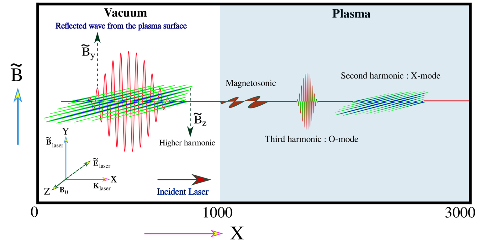
Table 1 presents laser and plasma parameters in normalized units. A set of possible values in standard units has also been provided. We have treated both electron and ion dynamics in our simulations with a reduced mass of ions $m_i=100m_e$ . For some cases, we have also treated the ions to be infinitely massive and acting merely as a stationary background. The inferences on harmonic generation were not altered for the two cases. A laser pulse with intensity $\approx 3 \times 10^{15}$
 W cm$^{-2}$
 (for normalized vector potential, $a_0=eE_l/m\omega _lc=0.5$
 ) and frequency $\omega _{l}= 0.4 \omega _{pe}$
 is incident normally from the left-hand side of plasma. The electric field of the laser $E_l$
 is chosen to be along $\hat {z}$
 for the O-mode configuration and along $\hat {y}$
 for the X-mode configuration. In figure 1 the O-mode configuration is depicted in a schematic representation. The longitudinal profile of the laser pulse is a polynomial function with rise and fall time of $100 \omega _{pe}^{-1}$
 which translates to $200$
 fs and it starts from $x=950 d_{e}$
 . The value of the external magnetic field is chosen to elicit magnetized response of electrons while ions remain unmagnetized at the laser frequency, i.e. $\omega _{ce}> \omega _{l}> \omega _{ci}$
 , where $\omega _{ci}$
 and $\omega _{ce}$
 are cyclotron frequencies of ion and electron, respectively, while $\omega _{l}$
 is the laser frequency. Absorbing boundary conditions are used for fields and particles. For an unmagnetized plasma (i.e. in the absence of an external magnetic field), the laser cannot penetrate inside the plasma. In the X-mode configuration, even in the overdense case, if the laser frequency lies in the passband of the magnetized plasma, it propagates inside and generates lower hybrid and magnetosonic excitation, as has been illustrated in some earlier works (Kumar et al. Reference Kumar, Shukla, Verma, Das and Kaw2019; Vashistha et al. Reference Vashistha, Mandal and Das2020a,Reference Vashistha, Mandal, Kumar, Shukla and Dasb). However, for the O-mode configuration, the laser cannot propagate inside the plasma if it is overdense. In this case, the laser light only penetrates the plasma up to the order of the skin depth. We observe that this is sufficient for the generation of harmonics in the O-mode configuration. For the higher frequency of harmonics that get generated, the plasma becomes underdense. In such a situation, the generated harmonic radiation is free to propagate inside the plasma.
Simulation parameters: in normalized units and possible values in standard units.

In our PIC simulation study, we have not included Coulomb collisions. The quiver velocity of electrons would be high at the laser intensities of $\sim 10^{15}$ W cm$^{-2}$
 considered in our study. We, therefore, feel that the collisions will not have any significant role to play (Dendy Reference Dendy1995). In our study, the initial temperature of electrons is assumed to be very low ($T_e = 0.05$
 eV). Such an assumption is valid because the temperature remains small compared to the typical oscillation energy of electrons in intense laser fields (Gibbon Reference Gibbon2005). Thus, the plasma temperature will not affect the harmonic generation mechanism presented here. We have done a comparative study of the effect of temperature on the generation of harmonics too (in § 3.3) which illustrates the above point.
3. Observations and discussion
It is well known that in the X-mode configuration, the EM radiation of the laser penetrates the plasma in the respective permitted passbands. In this case, bulk plasma can interact with the incident radiation although $\omega _l < \omega _{pe}$ . In the O-mode, however, the dispersion relation being identical to the unmagnetized case, there is no propagation when the EM wave frequency is smaller than the plasma frequency. The laser–plasma interaction, in this case, is thus confined only within the electron skin depth layer. The plasma within the skin depth responds to the Lorentz force acted upon by the electric and magnetic fields of the EM wave and the applied external magnetic field. The incident EM radiation has a finite spatial pulse profile in the longitudinal direction. The finite spatial profile of the laser pulse provides for an additional ponderomotive force to the plasma medium. We have chosen to work in the frequency domain (shown in table 1) for which the condition $\omega _{ci}<\omega _l<\omega _{ce}$
 is satisfied. Here, $\omega _l$
 defines the laser frequency and $\omega _{ce}$
 and $\omega _{ci}$
 represent the electron and ion cyclotron frequency, respectively. Thus, electrons would have a magnetized response to offer in the time period corresponding to a laser cycle, whereas ions would be unmagnetized. We now present various features of our observations in the following subsections.
3.1. Harmonic generation in O-mode configuration $({\boldsymbol{E}}_l \parallel {\boldsymbol{B}}_0)$

We first consider the case when the frequency of the incident laser pulse was chosen to be $0.4 \omega _{pe}$ and the polarization of the laser fields was considered to be in O-mode configuration, i.e. ${\boldsymbol {E}}_l \parallel {\boldsymbol {B}}_0$
 (in $\hat z$
 direction). Here, $\boldsymbol {E}_l$
 is the laser electric field and $\boldsymbol {B}_0$
 is the externally applied magnetic field. The transverse $\hat y$
 and $\hat z$
 components of the magnetic field, $B_y$
 and $B_z$
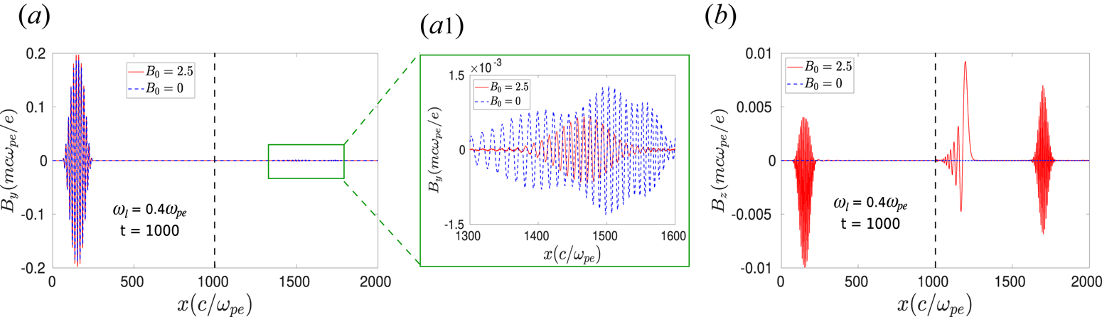
 , are shown by red solid lines for $B_0 = 2.5$
 at a particular instant of time $t = 1000$
 in figures 2(a) and 2(b), respectively. It is to be noted that at time $t = 0$
 , a laser pulse with EM fields $B_y$
 and $E_z$
 was set to propagate along the positive $\hat x$
 direction from the location $x = 950$
 . Thus, the structure in $B_y$
 present in the vacuum region ($x \approx 200$
 ) at $t = 1000$
 , as seen from 2(a), is associated with the reflected part of the incident laser propagating along the $-\hat x$
 direction. A small fraction of $B_y$
 is also present inside the bulk plasma, as depicted in the zoomed scale in 2(a1). We will identify this structure as the third-harmonic radiation (and the higher odd harmonics) in the following section. In 2(b), it is seen that the $\hat z$
 component of the oscillating magnetic field $B_z$
 which is not present before the laser beam impinges on the plasma surface, has been produced at a later time and exists in both vacuum and bulk plasma. There are two types of disturbances observed inside the bulk plasma, as can be seen from 2(b). One is the large-scale disturbance near the plasma surface, which will be identified as the magnetosonic perturbation, and the other is a disturbance moving with the faster group velocity. In the following discussion, we will show that this is the second-harmonic radiation (even harmonics) generated due to the interaction of laser pulse with plasma particles. The simulation observations for $B_0 = 0$
 are also depicted in figure 2 by blue dotted lines. It is seen that in this case, also the $\hat y$
 component of the magnetic field, i.e. $B_y$
 , is present in both reflected and transmitted radiations. However, no $\hat z$
 component of the magnetic field, i.e. $B_z$
 , is generated in this case, as can be seen in 2(b).
Transverse time-varying magnetic fields (a) $B_y$ and (b) $B_z$
 with respect to $x$
 are shown at a particular instant of time $t = 1000$
 (when the laser beam already gets reflected back from the system). In (a1), $B_y$
 , which exists inside the plasma, is shown on a different scale. Here, the black dotted line at $x = 1000$
 represents the plasma surface. It is to be noted that the EM fields $\boldsymbol {B_l}$
 and $\boldsymbol {E_l}$
 of the incident laser pulse are along the $\hat y$
 and $\hat z$
 directions, respectively. Red lines represent $B_0 = 2.5$
 with $E_l \parallel B_0$
 and blue dotted lines $B_0 = 0$
 .
.
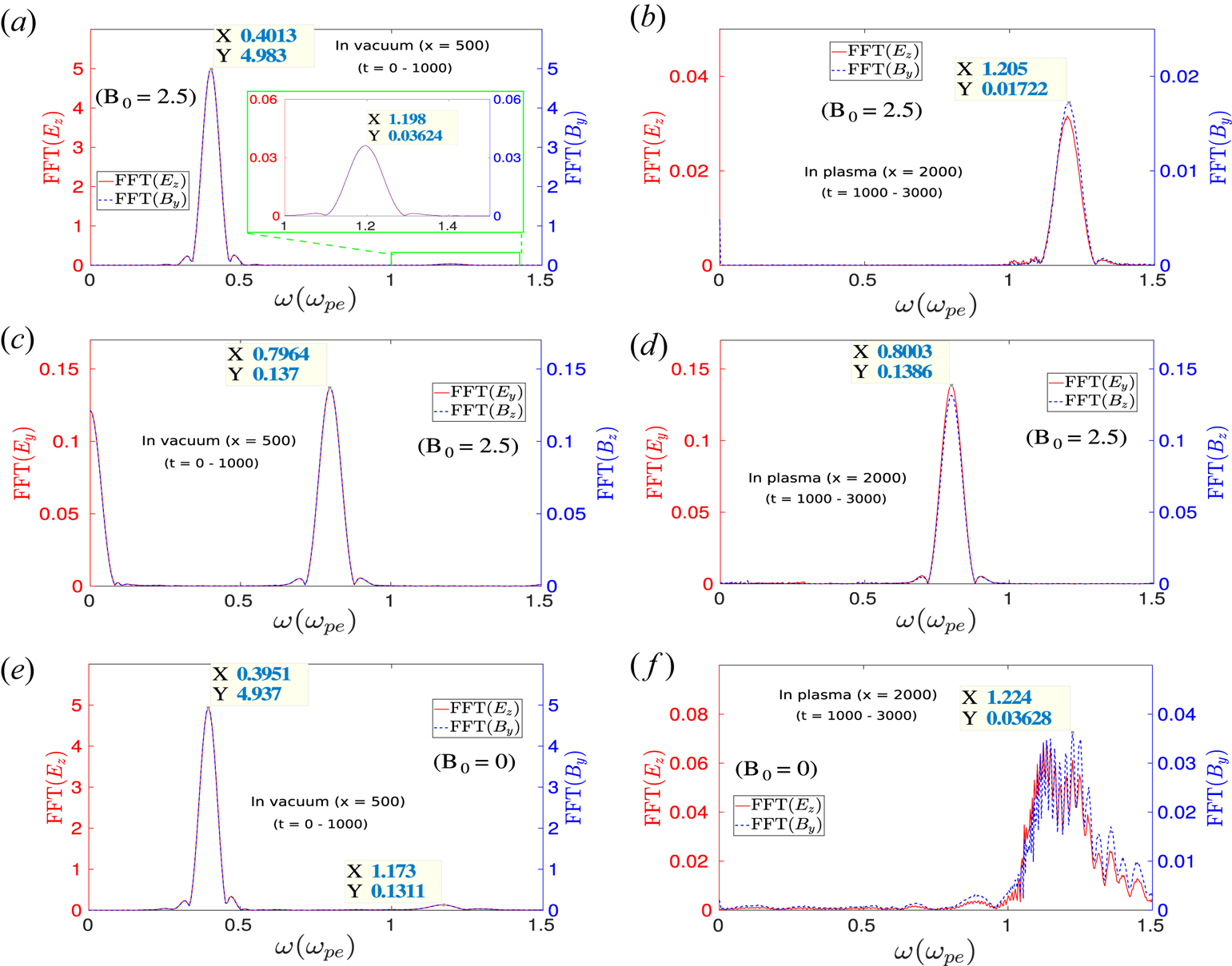
The time fast Fourier transform (FFT) of these reflected and transmitted radiations is shown in figure 3. The FFTs of $E_z$ and $B_y$
 at the location $x = 500$
 (vacuum) show two distinct peaks at frequencies $\omega \approx 0.4\omega _{pe}$
 and $\omega \approx 1.2\omega _{pe}$
 (figure 3a). It is important to recall that at $t = 0$
 , the incident laser pulse was located between $x= 750$
 and $950$
 . The first peak with higher power at the location $\omega \approx 0.4\omega _{pe}$
 is essentially the original laser pulse which has been reflected from the plasma surface, as the plasma is overdense. The second peak located at $\omega \approx 1.2\omega _{pe}$
 is the third-harmonic radiation. The third harmonic is also present inside the bulk plasma and has been demonstrated by carrying out the FFT in time for the $E_z$
 and $B_y$
 signals at the location $x = 2000$
 (plasma), as shown in figure 3(b). Thus, it is now clear that the small disturbance in $B_y$
 present inside the plasma, as shown in figure 2(a1), is essentially associated with the third-harmonic radiation. The FFTs of $E_y$
 and $B_z$
 in time at the locations $x = 500$
 and $2000$
 are shown in figures 3(c) and 3(d), respectively. The FFT at the location $x = 2000$
 (plasma), in 3(d), has been evaluated within a time window $t = 1000$
 to $3000$
 . This is to eliminate the slowly moving magnetosonic disturbance as shown in figure 2(b). It is seen that the frequency spectrum of $E_y$
 and $B_z$
 has a distinct peak at the location $\omega \approx 0.8\omega _{pe}$
 in both cases (vacuum and plasma). This ensures that the second-harmonic radiation has been generated and travels in both vacuum and plasma mediums. The observation of second and third harmonics in the reflected radiation in the presence of a transverse external magnetic field had been reported in an earlier study by Mu et al. (Reference Mu, Li, Sheng and Zhang2016). However, in our study, we have observed the harmonic radiations in both reflected and transmitted radiations, as shown in figure 3. In the case without an external magnetic field, the third harmonic (odd harmonics) shows up with polarization ($E_z$
 , $B_y$
 ) in both reflected and transmitted radiations, as shown in figure 3(e,f). It is to be noticed that, unlike a magnetized case, no harmonics with polarization ($E_y$
 , $B_z$
 ) are generated in the absence of an external magnetic field, as shown in figure 2(b). In the case with $B_0 = 0$
 , the existence of so-called selection rules for the polarization of harmonic generation reflected from an overdense plasma surface was predicted by Lichters et al. (Reference Lichters, Meyer-ter Vehn and Pukhov1996). Their study shows that for a normal incident linearly polarized laser, only the odd harmonics with linear polarization appear in the reflected radiation. The analogy of third-harmonic generation reported for the present study is the same as reported by Lichters et al. (Reference Lichters, Meyer-ter Vehn and Pukhov1996). However, here we have observed and characterized them in both reflected and transmitted radiations. It is interesting to note that we have shown the FFT of transverse electric and magnetic field components in each subplot as a pair. This is done to show the EM nature of harmonic radiations. It is also important to observe that the polarization of third-harmonic radiation is the same as that of the incident laser pulse. In contrast, the polarization of the second-harmonic radiation is different from that of the incident laser pulse. In § 3.3, we discuss the reason behind this.
Fourier transform of EM fields with time after the laser beam is reflected from the plasma surface. The FFT of $E_z$ and $B_y$
 with time in (a) vacuum ($x = 500$
 ) and (b) the bulk plasma ($x = 2000$
 ). (c,d) The same for the fields ($E_y$
 , $B_z$
 ). In (a)–(d), the external magnetic field ($B_0$
 ) is considered to be $2.5$
 . These FFTs clearly indicate that higher harmonics have been generated, and they are present in both vacuum and the bulk plasma. The time FFT of $E_z$
 and $B_y$
 without any external magnetic field ($B_0 = 0$
 ) in (e) vacuum and (f) plasma.
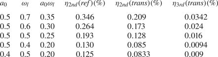
The conversion efficiencies of second and third harmonics are provided in table 2 for different values of $a_0$ ($=eE_l/m\omega _lc$
 ) and laser frequency $\omega _l$
 . The conversion efficiency has been calculated by taking the ratio of spatially integrated EM field energy of the harmonic to that of the incident laser pulse. We have observed that the conversion efficiency solely depends on the strength of the laser fields for a given magnetic field. Keeping $a_0$
 constant when we increase $\omega _l$
 , field strength increases, and so do the efficiencies of the harmonics. On the other hand, as we keep the value of $(a_0\omega _l)$
 constant for a different combination of $a_0$
 and $\omega _l$
 , the field strength of the incident laser pulse remains the same, and so does the conversion efficiency. This is clearly shown in table 2.
Conversion efficiencies of harmonics in O-mode configuration of incident laser pulse for $B_0=2.5$ .
.
3.2. Harmonic generation in X-mode configuration $(\boldsymbol{E}_l \perp \boldsymbol{B}_0)$

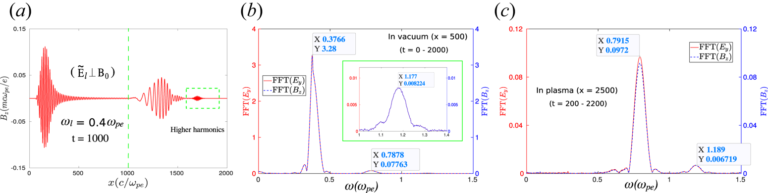
The higher harmonics can also be observed for the case when the polarization of the incident laser pulse is chosen to be in the X-mode configuration, i.e. ${\boldsymbol {E}}_l \perp {\boldsymbol {B}}_0$ . This is clearly illustrated in figure 4. A laser pulse with frequency $0.4 \omega _{pe}$
 was set up initially ($t = 0$
 ) to propagate in the $\hat x$
 direction from the location $x = 950$
 . In this case also, the external magnetic field $B_0$
 has been chosen to be $2.5$
 and applied in the $\hat z$
 direction. It is to be noticed that for our chosen values of system parameters, the frequency of the incident laser pulse lies between the left-hand cutoff ($\omega _L = 0.376$
 ) and upper hybrid frequency ($\omega _{UH} = 2.7$
 ). Thus, the incident laser pulse with polarization in the X-mode configuration will match the passband of the plasma X-mode dispersion curve. As a result, a significant part of the incident laser pulse penetrates inside the bulk plasma. This is clearly illustrated in figure 4(a) where we show the $z$
 component of the magnetic field $B_z$
 as a function of $x$
 at a particular instant of time $t = 1000$
 . It is also seen that a part of the incident pulse gets reflected from the vacuum–plasma interface and propagates in the $-\hat x$
 direction in the vacuum. The other part of the incident laser radiation penetrates the plasma surface and propagates through the medium. It can be observed that a small disturbance, as highlighted by the dotted rectangular box in figure 4(a), is also present, which moves with a higher group velocity in the plasma medium. These are essentially the higher harmonics generated by the plasma. The FFTs in time for this signal of the transverse fields $E_y$
 and $B_z$
 in figure 4(b,c) corroborate this. The FFTs of $E_y$
 and $B_z$
 inside the plasma ($x = 2500$
 ), as shown in figure 4(c), are evaluated within a time window $t = 200$
 to $2200$
 . This choice eliminates the originally transmitted laser pulse with frequency $0.4\omega _{pe}$
 (having higher power) from the frequency spectrum. Two distinct peaks observed at $\omega \approx 0.8\omega _{pe}$
 and $1.2\omega _{pe}$
 in figure 4(b,c) correspond to the second and third harmonics, respectively. It is interesting to notice that unlike the previous case (O-mode configuration), here the polarization of the higher harmonics, both second and third, is the same as that of the incident laser pulse.
The generation of higher harmonics is depicted here for the case where the polarization of incident laser has been chosen to be in the X-mode configuration, i.e. $\boldsymbol {\tilde {E}}_{l} \perp \boldsymbol {B}_0$ . Here, we have considered $B_0 = 2.5$
 . (a) The EM part of the magnetic field along $\hat z$
 , $B_z$
 , at a particular instant of time $t = 1000$
 . (b) The FFT of $E_y$
 and $B_z$
 at the location $x = 500$
 (vacuum). It is clearly seen that in addition to the original reflected laser field ($\omega \approx 0.4$
 ), higher harmonics ($\omega \approx 0.8, 1.2$
 ) are also present in the reflected radiation. (c) The existence of these higher harmonics inside the bulk plasma, where the FFTs have been performed at the location $x = 2500$
 .
.
3.3. Mechanism of harmonic generation in a magnetized plasma
Let us now understand the mechanism of the harmonic generation. The fundamental mechanism of high-order harmonic generation at the vacuum–magnetized plasma interface has been previously studied by Mu et al. (Reference Mu, Li, Sheng and Zhang2016). In the present work, we briefly discuss the same extending it for both O- and X-mode configurations of the incident laser pulse. Additionally, we have also developed a simple approximate mathematical model for a qualitative description of the observed characteristics in both O- and X-mode configurations, which is provided in Appendix A.
When a laser pulse with O-mode configuration, i.e. ${\boldsymbol {E}}_l \parallel {\boldsymbol {B}}_0$ , is incident on the vacuum–plasma interface, plasma particles will experience a force ($\propto \tilde {v}_{z}\tilde {B}_{l}\exp ({\textrm {i}2\omega _l t)}$
 ) due to the Lorentz force (${\boldsymbol {v}} \times {\boldsymbol {B}}_l$
 ) along the $\hat x$
 direction. Here, ${\boldsymbol {v}}$
 is the particle quiver velocity initiated due to the laser electric field $\boldsymbol {E_l}$
 in $\hat z$
 . As a result, plasma electrons wiggle, forming an oscillating current at the surface of the plasma in the $\pm \hat x$
 direction with a frequency twice the incident laser frequency (equation (A10a,b)). This can also be understood by recalling that in the intense EM fields of the incident laser, electron motion would initially follow the well-known ‘figure-of-eight’ path, which contains a transverse component with a frequency $\omega _l$
 and a longitudinal component with frequency $2\omega _l$
 (Teubner & Gibbon Reference Teubner and Gibbon2009). The electrons being magnetized in the presence of the external magnetic field $B_0\hat {z}$
 , revolve in the $x$
 –$y$
–$y$ plane. Thus, the oscillatory motion of electrons along $\hat x$
 generated by the process discussed above is coupled with the motion along $\hat {y}$
 , having the same frequency. Consequently, an oscillating current with a frequency twice the laser frequency is produced in the $\hat y$
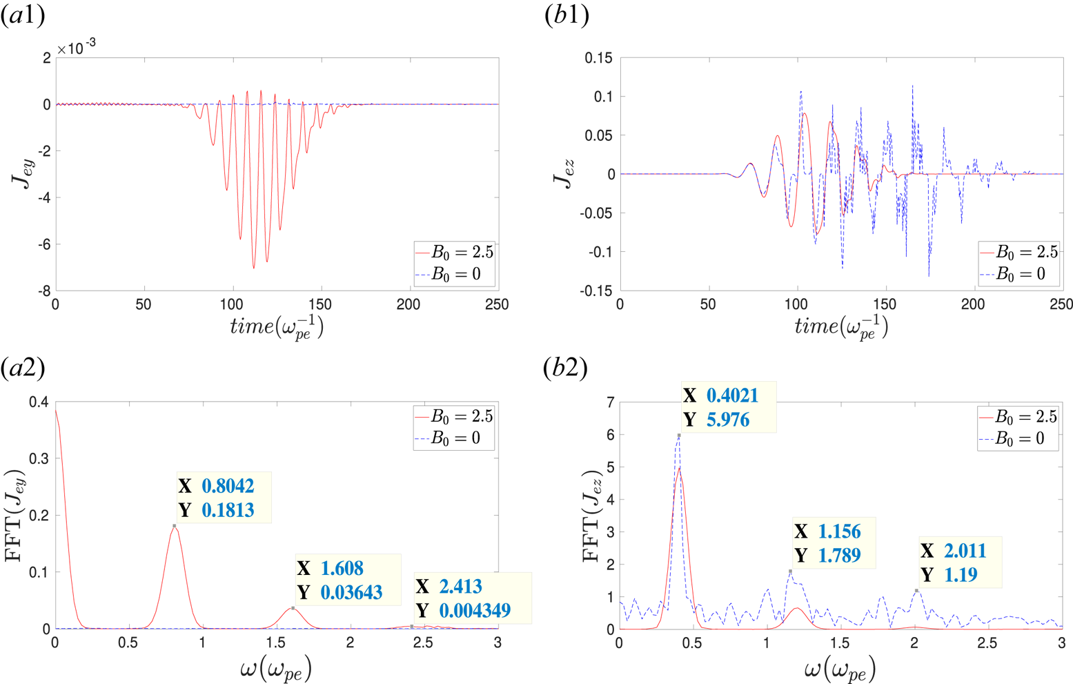
 direction, as shown in figure 5(a1,a2). This acts as an oscillating current sheet antenna and radiates EM waves with fields $\tilde {E}_y$
 and $\tilde {B}_z$
 propagating along both $\pm \hat x$
 directions. These are the second harmonics that have been captured in our simulations in both vacuum and plasma regimes. It is easy to understand that the oscillating current sheets in the $\hat y$
 direction might have all the even higher harmonics depending upon the strength of the nonlinearity involved in the electron dynamics. In our simulations, we have captured up to the sixth harmonic and can be easily seen in the FFT of $J_{ey}$
 in figure 5(a2).
The time evolution of (a1) $y$ component and (b1) $z$
 component of electron currents $J_{ey}$
 and $J_{ez}$
 at the vacuum–plasma interface ($x = 1000$
 ), respectively. The FFTs of (a2) $J_{ey}$
 and (b2) $J_{ez}$
 . Here, the red solid lines and blue dotted lines represent the cases with $B_0 = 2.5$
 and $B_0 = 0$
 , respectively.
In addition, the electron motion along $\hat x$ will couple to the laser magnetic field $\tilde {B}_l$
 (which is along $\hat y$
 for O-mode configuration). As a result, it will create an oscillating current sheet along $\hat z$
 with a frequency three times the laser frequency and also at higher odd harmonic values, as shown in figure 5(b1,b2). Thus, another radiation will be produced propagating in the $\pm x$
 direction, but, in this case, the EM fields associated with this radiation are $\tilde {E}_z$
 and $\tilde {B}_y$
 . It is to be noticed that ideally, all the odd higher harmonics might be present in $J_{ez}$
 . In our simulations, we have identified up to the fifth harmonic, as shown in figure 5(b2). It is to be noticed that the external magnetic field is necessary to generate the $\hat y$
 component of surface current $J_{ey}$
 , oscillating with the even harmonic frequencies, producing the even higher-harmonic EM radiations. This is shown by red solid and blue dotted lines in figure 5(a1,a2) and is also consistent with the approximate mathematical expression of $J_{ey}$
 in (A10a,b). On the other hand, the $\hat z$
 component of surface current, i.e. $J_{ez}$
 , oscillating with odd harmonic frequencies is produced only due to the nonlinear electron dynamics in the laser fields and does not require any external magnetic field (Bulanov et al. Reference Bulanov, Naumova and Pegoraro1994; Lichters et al. Reference Lichters, Meyer-ter Vehn and Pukhov1996; Teubner & Gibbon Reference Teubner and Gibbon2009), as shown in figure 5(b1,b2). This is also apparent from the expression of $J_{ez}$
 in (A13).
For the laser polarization in the X-mode configuration, the magnetic field $\tilde {B}_l$ of the laser is parallel to ${B_0}$
 (along $\hat z$
 ). For this case, using similar arguments, both second and third harmonics (in fact, all the high harmonics) will be generated for which the EM fields are $\tilde {E}_y$
 and $\tilde {B}_z$
 . Thus, the generated harmonic radiation also has the X-mode configuration. This is exactly what we have observed in our simulations, as shown in figure 4.
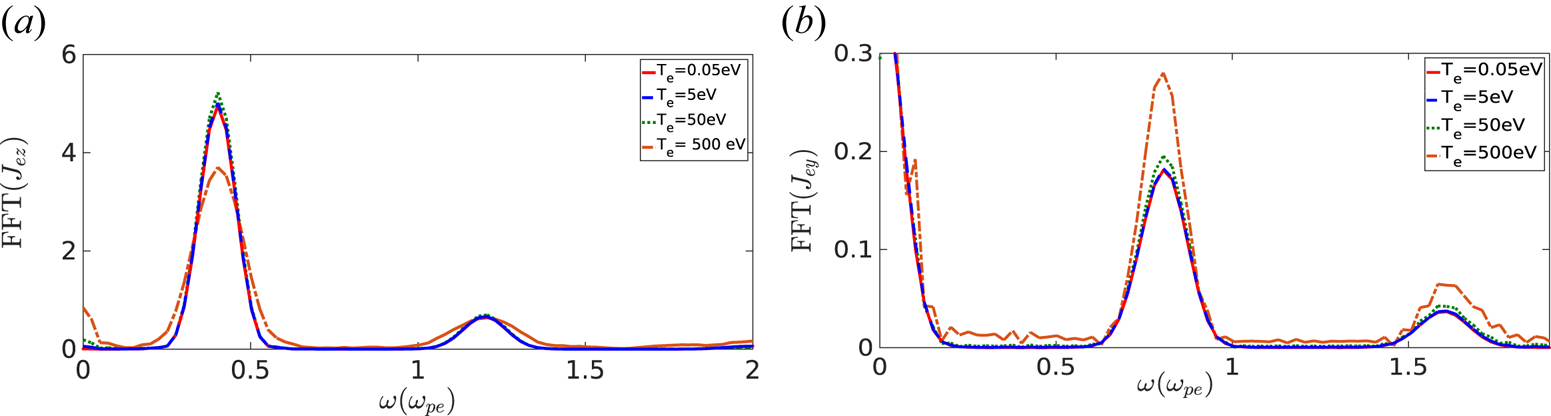
As mentioned in § 2, in most of our simulation studies we have considered the electron temperature to be very low ($T_e = 0.05$ eV). However, we have also done a comparative study by considering different values of electron temperature to check if the fundamental mechanism of harmonic generation has any dependence on the plasma temperature. The time FFTs of surface currents $J_{ez}$
 and $J_{ey}$
 are shown for different values of electron temperature ($T_e = 0.05$
 –500 eV) in figures 6(a) and 6(b), respectively. It is seen that surface currents oscillating with high harmonic frequencies have been generated in all cases. There is no significant change observed in the generation of high-harmonic radiations for different values of electron temperature.
The FFTs in time for (a) $\hat {z}$ component of surface current $J_{ez}$
 and (b) $\hat {y}$
 component of surface current $J_{ey}$
 at the vacuum–plasma interface ($x=1000 c/\omega _{pe}$
 ) for different electron temperatures ($T_e=0.05$
 , 5, 50 and 500 eV).
3.4. Effect of external magnetic field on harmonic generation
We have shown in the previous section that the generation of harmonics depends on the surface current oscillations, and odd harmonics can be generated even when there is no external magnetic field. However, it has been shown that an external magnetic field is necessary to generate higher even harmonics. In this section, we show that the amplitude of harmonics (both even and odd) actually has a strong dependence on applied external magnetic fields.
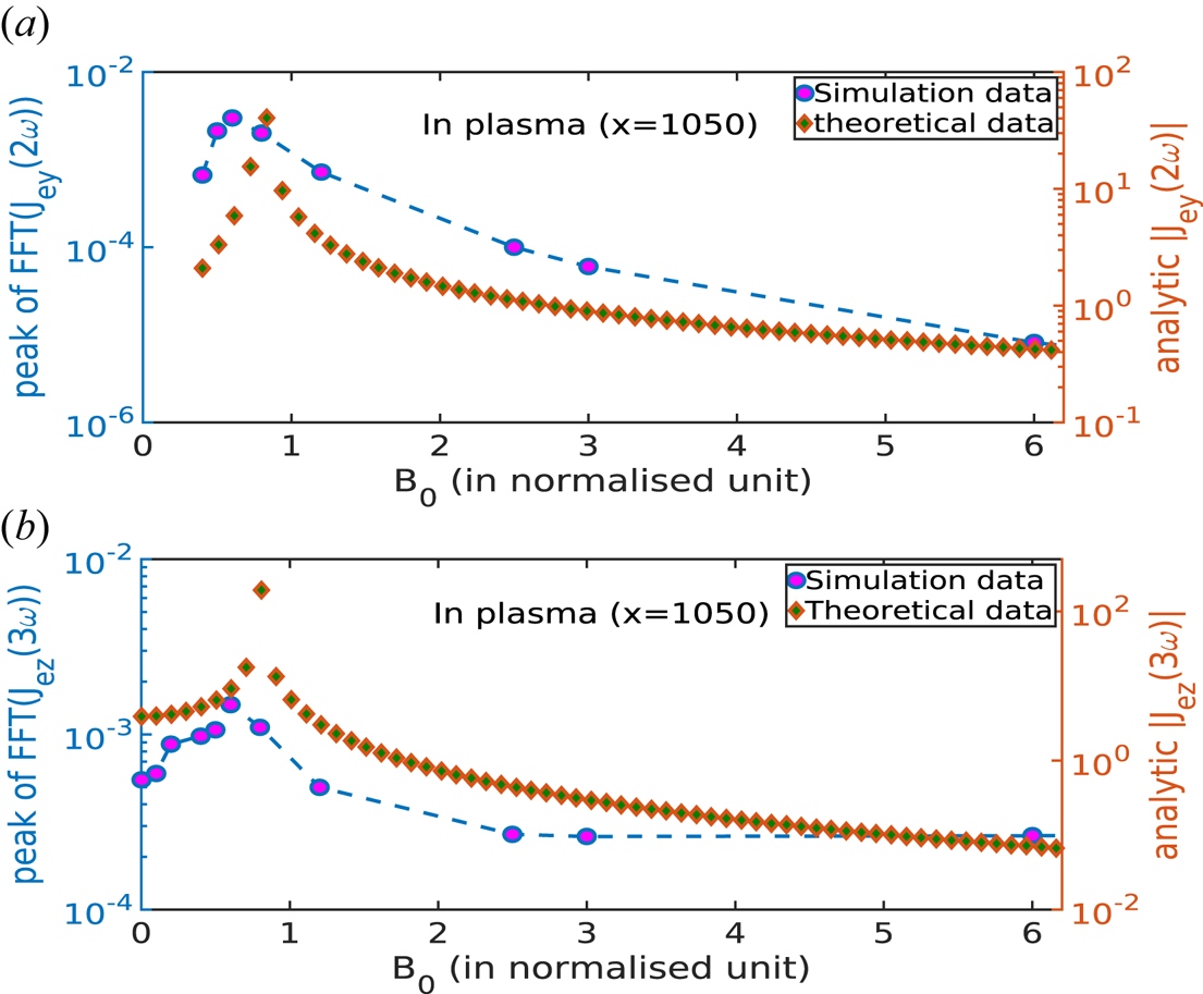
For this analysis, we have done a comparative study by simulating the same geometry with $\omega _l=0.4\omega _{pe}$ for different values of the external magnetic field. In each run, we have obtained the amplitude (peak value) of FFT from time-series data of $J_{ey}$
 and $J_{ez}$
 corresponding to the second- and third-harmonic frequency, respectively. Next, we have calculated the absolute value of second- and third-harmonic current density from the approximated model given in Appendix A, i.e. (A10a,b) and (A13), for different magnetic field values. We have plotted these two quantities as a function of the external magnetic field $B_0$
 as shown in figure 7. One can observe that the trends are similar for quantities obtained from simulation and the theoretical model. This plot provides a qualitative understanding of the mechanism presented in this paper. This observation also establishes that harmonic generation in plasma is boosted in the presence of an external magnetic field. There is an optimum value of the magnetic field for which better efficiency of harmonic generation can be found, and this value is where $\omega _{ce} \rightarrow 2\omega _{l}$
 .
.
(a) The peak value of the FFT spectrum of $J_{ey}$ corresponding to the second-harmonic frequency and theoretical value of $|{J_{ey}}|$
 obtained from (A10a,b). (b) The peak value of the FFT spectrum of $J_{ez}$
 corresponding to the third-harmonic frequency and theoretical value of $|{J_{ez}}|$
 obtained from (A13).
3.5. Characterization of harmonics
We now analyse in further detail and characterize the high-harmonic radiations. As has been shown previously, these higher harmonics can be observed for the laser polarization in both O-mode (${\boldsymbol {E}}_l \parallel {\boldsymbol {B}}_0$ ) and X-mode (${\boldsymbol {E}}_l \perp {\boldsymbol {B}}_0$
 ) configurations. We consider here the observations corresponding to the O-mode configuration. As discussed in previous sections, the higher-harmonic radiations are EM. Thus, in vacuum, these radiations will travel with the speed of light, i.e. the frequency and wavenumber (in normalized units) will have the same values. On the other hand, when they propagate through the plasma medium, they will have to follow the appropriate dispersion relation of that medium.
Thus, the group velocity and the phase velocity of these radiations will have different values depending upon the dispersion relation. These properties are clearly shown in figure 8. The spatial FFTs of the transverse fields ($E_z$ , $B_y$
 ) for vacuum and bulk plasma are shown in figures 8(a) and 8(b), respectively. It is clearly seen from figure 8(a) that, as expected, the reflected laser pulse ($\omega _l = 0.4$
 ) and the third-harmonic radiation ($\omega \approx 1.2$
 ) are associated with the wavenumbers $k_x \approx 0.4$
 and $k_x \approx 1.2$
 , respectively, as they travel in vacuum. On the other hand, the spectrum of the spatial FFTs of $E_z$
 and $B_y$
 in the bulk plasma region shows a distinct peak at a particular value of $k_x \approx 0.67$
 . It is interesting to realize that the third-harmonic radiation is associated with the transverse electric field ($E_z$
 ) parallel to the external magnetic field $B_0$
 and travelling perpendicular to $B_0$
 . Thus, it matches the condition of plasma O-mode. We have evaluated the theoretical dispersion curve for the O-mode for our chosen values of system parameters, as shown in figure 8(e). It is seen that the value of wavenumber corresponding to the frequency $\omega = 1.2$
 is approximately equal to $0.66$
 . Thus, it matches well with the properties of third-harmonic radiation observed in our simulation inside the bulk plasma region.
Fourier transforms in space of the EM fields after the laser beam is reflected from the vacuum–plasma interface. The FFT of ($E_z$ , $B_y$
 ) along $\hat x$
 at time $t = 600$
 and $1600$
 for (a) vacuum and (b) bulk plasma. (c,d) The same for the fields ($E_y$
 , $B_z$
 ). Dispersion curves (Boyd, Boyd & Sanderson Reference Boyd, Boyd and Sanderson2003) of (e) O-mode and (f) X-mode for the chosen values of the system parameters of this study.

The FFTs of transverse fields $E_y$ and $B_z$
 in space associated with the second-harmonic radiation are depicted in figures 8(c) and 8(d) for vacuum and bulk plasma, respectively. The FFT spectrum reveals that the second-harmonic radiation ($\omega \approx 0.8$
 ) propagates with a finite wavenumber in a vacuum, $k_x \approx 0.8$
 , which is expected as it has to travel with the speed of light. On the other hand, inside the plasma, it is associated with a different wavenumber $k_x \approx 0.76$
 . The theoretical model analysis again affirms that this second-harmonic radiation matches the condition for plasma X-mode and propagates through the passband lying between left-hand cutoff ($\omega _L$
 ) and upper hybrid frequency ($\omega _{UH}$
 ) of the X-mode dispersion curve. This is demonstrated in figure 8(f).
The mode analysis of harmonic radiations has a direct significance in the sense that we can now have control over the excitation of these radiations inside the plasma medium. For a given set of plasma parameters, if we change the value of $B_0$ , the dispersion curves of the plasma modes (figure 8) will be modified accordingly. Thus, the value of $B_0$
 determines whether harmonic radiation with a particular frequency generated at the vacuum–plasma interface will be able to transmit inside the plasma or not. Alternatively, if the value of $\omega _l$
 is changed, the frequency of the higher harmonics will also be modified accordingly. Thus, there might be some situations where these harmonics will not be allowed to pass through the plasma medium for a particular value of $B_0$
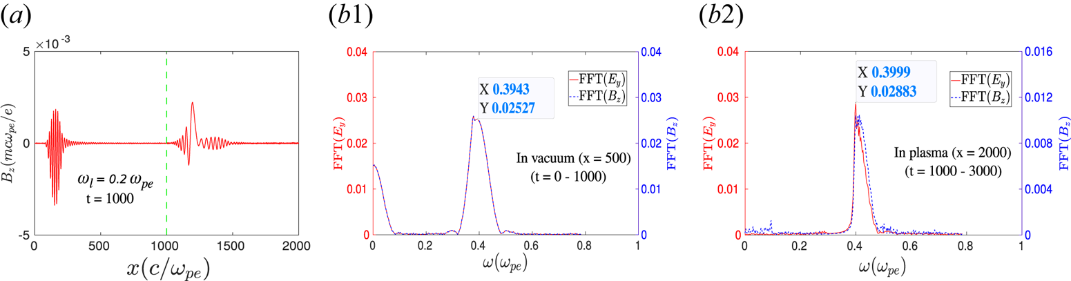
 . For instance, we have considered a particular case where the frequency of the incident laser pulse is chosen to be $0.2 \omega _{pe}$
 and all other system parameters have been kept the same as for the previous case. It has been observed that the second-harmonic radiations initiated at the vacuum–plasma interface are travelling in both vacuum and plasma. This is clearly demonstrated in figure 9(a). It is to be noticed that the frequency of the second-harmonic radiation, which happens to be $0.4\omega _{pe}$
 in this case (figure 9b1,b2), is still higher than the left-hand cutoff $\omega _L = 0.376$
 , and thus lies within the passband region between $\omega _L$
 and $\omega _{UH}$
 . Hence, the second-harmonic radiation is allowed to pass through the plasma. On the other hand, the third-harmonic radiation, which has the O-mode characteristics, will have a frequency $0.6\omega _{pe}$
 . Thus, in this particular case, the third-harmonic radiation lies below the cutoff ($\omega = \omega _{pe}$
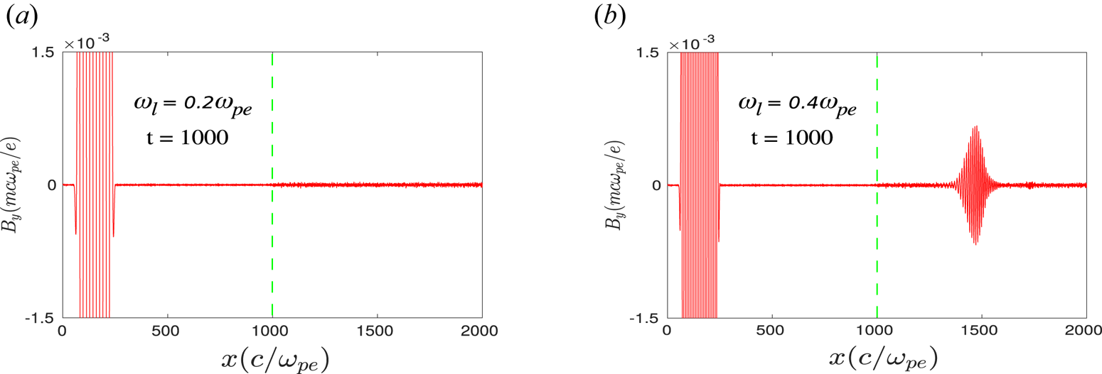
 ) of the O-mode dispersion curve and is forbidden to propagate inside the plasma. This is clearly illustrated in figure 10. In figures 10(a) and 10(b), we show the $y$
 component of the transverse magnetic field $\tilde {B}_y$
 at a particular instant of time $t = 1000$
 for two different incident laser frequencies $\omega _l = 0.2\omega _{pe}$
 and $0.4\omega _{pe}$
 , respectively. It is seen that for $\omega _l = 0.2\omega _{pe}$
 (10a), EM field $\tilde {B}_y$
 of the incident laser pulse has been reflected from the vacuum–plasma interface and no signal of $\tilde {B}_y$
 exists inside the plasma. Whereas, for $\omega _l = 0.4\omega _{pe}$
 (10b), a part of $\tilde {B}_y$
 is also present inside the plasma and which is associated with the third-harmonic radiation, as also demonstrated in § 3.1.
(a) The $z$ component of the magnetic field $B_z$
 (EM) with respect to $x$
 at time $t = 1000$
 . The green dotted line at the location $x = 1000$
 represents the vacuum–plasma interface. The FFTs of ($E_y$
 , $B_z$
 ) at the locations (b1) $x = 500$
 and (b2) $x = 2000$
 in the frequency domain clearly demonstrate that the second harmonic is present in both reflected and transmitted radiations, respectively.
The $y$ component of magnetic field $B_y$
 (EM) with respect to $x$
 at a particular instant of time $t = 1000$
 for incident laser frequency (a) $\omega _l = 0.2$
 and (b) $\omega _l = 0.4$
 . In both cases, the polarization of the incident laser has been chosen to be in O-mode configuration, i.e. $\boldsymbol {\tilde {E}}_{l} \parallel \boldsymbol {B}_0$
 (along $\hat z$
 ), and the value of $a_0$
 is considered to be 0.5. Here, the green dotted line at $x = 1000$
 represents the vacuum–plasma interface.
It is straightforward that in the presence of an external magnetic field $B_0$ , a plasma wave with electric field ${\boldsymbol {E}} \perp {\boldsymbol {B}}_0$
 and propagation vector ${\boldsymbol {k}} \perp {\boldsymbol {B}}_0$
 (X-mode configuration) always tends to be elliptically polarized instead of plane-polarized (Chen Reference Chen1984). That is, when an EM wave propagates through the plasma, an electric field component parallel to the propagation direction will also be present. The wave, therefore, has both EM and electrostatic features. In our study, the observed second-harmonic radiation is associated with an electric field perpendicular to $B_0$
 and propagates along $\hat x$
 , as shown in previous sections. Thus, an electric field component along $\hat x$
 , $\tilde {E}_x$
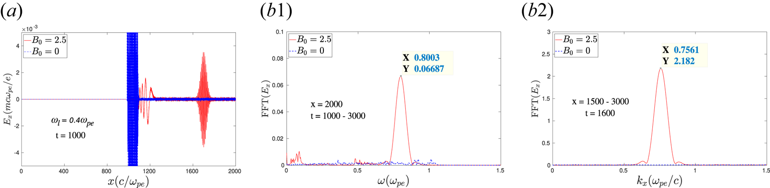
 , is also expected to be present and will be travelling along with the second-harmonic EM radiation. This is clearly depicted in figure 11(a). The $E_x$
 field profile is seen to be associated with the second-harmonic radiation. The Fourier spectra of this particular profile in both the $\omega$
 domain and $k$
 -space also show the same characteristic properties as the EM second-harmonic radiation, as is shown in figure 11(b1,b2). It is to be noticed that no $\hat x$
 component of electric field ($E_x$
 ) is observed inside the bulk plasma for the case without an external magnetic field, as is shown by blue dotted lines in figure 11. This is consistent with the results discussed in §§ 3.1 and 3.3. In this case, $E_x$
 is present only at the vacuum–plasma interface where the disturbances are made due to the ponderomotive pressure of the incident laser pulse. It cannot propagate inside the bulk plasma without an external magnetic field. It should be noted that the odd harmonics that are generated and present inside the bulk plasma for $B_0 = 0$
 (figure 2) can also induce longitudinal electric field $E_x$
 . However, this will be negligible for $B_0 = 0$
 as the longitudinal electric field will, in this case, get generated by the coupling of dynamics of electrons in the electric and magnetic field of the harmonic EM wave radiation (i.e. $\boldsymbol {E}_{nh}\times \boldsymbol {B}_{nh}$
 , where $n$
 represents the order of harmonic). Since the intensity of the harmonic radiation is typically much weaker, this effect will be very small compared to $E_x$
 that gets generated by the coupling of the electric field of the harmonic radiation with the external magnetic field. This is clearly illustrated in figure 11.
(a) The longitudinal electric field $E_x$ with respect to $x$
 at a particular instant of time $t = 1000$
 . The FFTs of $E_x$
 in (b1) the frequency domain and (b2) $k$
 -space. Here, the red solid lines and blue dotted lines represent the cases with $B_0 = 2.5$
 and $B_0 = 0$
 , respectively.
We also observe from figure 11(a) that a large-scale disturbance (red solid line) is present in $E_x$ near the plasma–vacuum interface for $B_0 = 2.5$
 . Such a disturbance has also been observed in the transverse fields $E_y$
 and $B_z$
 , as shown in figure 2(b). This fluctuation is EM but becomes elliptically polarized in the presence of an external magnetic field $B_0$
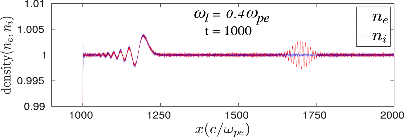
 , as discussed earlier. It is also observed that this disturbance travels with a much slower velocity than the higher-harmonic radiation present in the system. Such a disturbance has also been observed in both electron and ion density profiles, as can be seen in figure 12. The normalized density profiles of electrons and ions at a particular instant of time $t = 1000$
 are shown by the solid red line and blue dotted line, respectively, in figure 12. A spatial electron density profile travels along with the generated second-harmonic pulsed structure wave and is thus associated with it. As the second-harmonic frequency is much higher than the ion response time scale, this structure appears only in the electron density profile, not in that of ions. On the other hand, near the plasma surface, the fluctuations are present in both electron and ion density profiles, and they are almost identical. These fluctuations are associated with low-frequency magnetosonic perturbations. They are initiated due to the ponderomotive force associated with the finite pulse width of the laser. However, for the choice of infinitely massive ions, these magnetosonic perturbations do not appear. Such a disturbance has also been reported in a recent study by Vashistha et al. (Reference Vashistha, Mandal and Das2020a) for the X-mode configuration. We confirm that this is also present in the O-mode configuration.
Electron and ion density fluctuations are shown by red solid and blue dotted lines, respectively. Here, the external magnetic field $B_0$ is considered to be $2.5$
 .
.
4. Summary
We have shown that the interaction of a laser beam with a magnetized plasma has interesting and rich facets. The O-mode geometry, which is typically considered to exhibit unmagnetized plasma response, has certain distinctive features. Specifically, we have demonstrated the generation of harmonics in a magnetized plasma even in the O-mode configuration for the overdense plasma regime. The dynamics of a laser pulse interacting with plasma has been followed using one-dimensional PIC simulations with OSIRIS 4.0. A laser pulse coming from a vacuum is chosen to fall on an overdense plasma medium ($\omega _l<\omega _{pe}$ ) in the presence of an externally applied magnetic field. The dynamical mechanisms leading to higher-harmonic generation in both O-mode (${\boldsymbol {E}}_l \parallel {\boldsymbol {B}}_0$
 ) and X-mode (${\boldsymbol {E}}_l \perp {\boldsymbol {B}}_0$
 ) configurations have been demonstrated and analysed. It has been shown that when the incident laser has polarization in the O-mode configuration, higher even harmonics will be produced in the X-mode configuration, and odd harmonics in the O-mode configuration. Whereas both even and odd harmonics will be produced in the X-mode configuration for the incident laser pulse in the X-mode configuration. A comparison of simulation results with and without an external magnetic field has been provided and discussed. The required conditions for the propagation of the harmonic radiation inside the plasma have been identified. Our study reveals that the conversion efficiency for harmonic generation increases with laser intensity. We have also shown that the conversion efficiency has a strong dependence on the externally applied magnetic field. There is an optimum value of the magnetic field for which the amplitude of harmonics is maximum. Our study also demonstrates a conversion efficiency of about $1.77\,\%$
 for the second harmonic for a laser intensity of $a_0=0.5$
 and $B_0=0.6$
 , which is higher than the previously reported value for the analytical studies done in the context of magnetized plasma (Jha et al. Reference Jha, Mishra, Raj and Upadhyay2007; Ghorbanalilu Reference Ghorbanalilu2012). We feel that this can be improved further by appropriate tailoring of the plasma and magnetic field profiles.
Appendix A. Surface current oscillation in magnetized configuration
We demonstrate the possible generation of harmonics by surface electron currents, which would become excited by the laser field falling on an overdense plasma target in both O- and X-mode configurations. The spatial variation along $x$ is ignored for simplicity.
A.1. Surface current oscillation in O-mode configuration
In the O-mode configuration of incident laser waves, we have external magnetic fields and EM fields of an incident wave as follows:

The electron velocity is expanded in terms of various orders in the laser field amplitude as

From the Lorentz force equation we obtain for electrons

Balancing the first-order linear term in (A3) we obtain for the $\hat {z}$ component


The $x$ and $y$
 components represent the gyromotion and depend on the thermal velocity of electrons and are independent of the laser field.
For a cold plasma this can be ignored compared to the quiver velocity of the electron in the laser field. Thus, for the O-mode configuration ($\boldsymbol {\widetilde {E_1}} \perp \boldsymbol {B_0}$ ), $\tilde {v}_{x}^{(1)}$
 and $\tilde {v}_{y}^{(1)}$
 can be neglected.
The second-order term from (A3) gives


From the coupled expressions in (A7a,b), we will get

Here, $\omega _c = {eB_0}/{m}$ . Separating the time dependence we have

Solving (A8a,b), we obtain the expressions of the $x$ and $y$
 components of current as

Equation (A10a,b) represent the expression of currents in the $x$ –$y$
–$y$ plane oscillating with a frequency twice that of the incident wave (second harmonic). This oscillating current acts as an antenna and radiates EM radiation at the second-harmonic frequency.
Similarly, various components of the third-order velocity terms in (A3) obey

Equation (A11a,b) represents the cyclotron motion in the plane ($x$ –$y$
–$y$ ) perpendicular to $B_0$
 with an amplitude associated with the third-order correction of perpendicular velocity which can only have a thermal contribution. Thus, as mentioned previously, we can neglect this for our case.
The $z$ component of (A3) for third-order terms will give
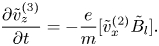
Using the expression of $\tilde {v}_{x}^{(2)}$ from (A10a,b), it can be shown that

Equation (A13) represents the $z$ component of current $\tilde {J}_z$
 oscillating with frequency $3\omega _{l}$
 (third harmonic).
It is to be noted that for the O-mode configuration of the incident wave, the second-harmonic radiation has polarization in the $x$ –$y$
–$y$ plane ($\tilde {J}_x$
 and $\tilde {J}_y$
 ) and the polarization of the third-harmonic radiation is along $\hat z$ $(\tilde {J}_z$
 ). If we calculate for all the higher-order terms, it can be shown that for the O-mode configuration, all the even harmonics will have polarization in the $x$
 –$y$
–$y$ plane and all the odd harmonics will have polarization along $\hat z$
 . This has also been observed in our simulation, as shown in figure 5.
A.2. Surface current oscillation in X-mode configuration
In the X-mode configuration of incident laser waves, we have the directions of external magnetic fields and EM fields of incident waves as follows:

We calculate the expression of higher-order terms of currents using (A3) and (A14a–c).
Solving for the first-order term of (A3):

The solutions of (A15a–c) can be written as

The second-order terms of (A3) can be expressed as

Equation (A17a–c) can be expressed as second-order differential equations as follows:

and

We can solve (A18) and (A19) using the expressions in (A16a–c). The solutions can be expressed as follows:

Here,

From (A20a,b) we can obtain the $x$ and $y$
 components of current oscillating with frequency $2\omega _{l}$
 (second harmonic), given by

Similarly, the third-order terms of (A3) can be expressed as

From (A23a–c), we can write

and

Solving (A24) and (A25) using the expression of $\tilde {v}_{x}^{(2)}$ and $\tilde {v}_{y}^{(2)}$
 given in (A20a,b), we can get

Here, the expressions of $F_3$ and $F_4$
 can be shown as

Equation (A26a,b) represents the $x$ and $y$
 components of currents oscillating with frequency $3\omega _{l}$
 (third harmonic). It is to be noted that, unlike the O-mode configuration, in this case we can get all the higher harmonics to be in the $x$
 –$y$
–$y$ plane. This has also been observed in our simulations.
Acknowledgements
The authors thank IIT Delhi HPC facility for computational resources. The authors would like to acknowledge the OSIRIS Consortium, consisting of UCLA and IST (Lisbon, Portugal) for providing access to the OSIRIS 4.0 framework which is the work supported by NSF ACI-1339893.
Editor Luís O. Silva thanks the referees for their advice in evaluating this article.
Declaration of interest
The authors report no conflict of interest.
Funding
This research work was supported by a J.C. Bose fellowship grant (A.D.; grant number JCB/2017/000055/SSC) from the Department of Science and Technology (DST), Government of India and the Core Research Grant (A.D.; grant number CRG/2018/000624) of the Science and Engineering Research Board (SERB), Government of India.
Author contributions
S.M. and A.D. planned the research; S.M. derived the theory and performed the simulations; S.M., D.M., A.V. and L.P.G. analysed the results; S.M., D.M., A.V., L.P.G. and A.D. interpreted the results; S.M., D.M., A.V. and A.D. wrote the manuscript; A.D. supervised the research.


 Open access

