

Introduction
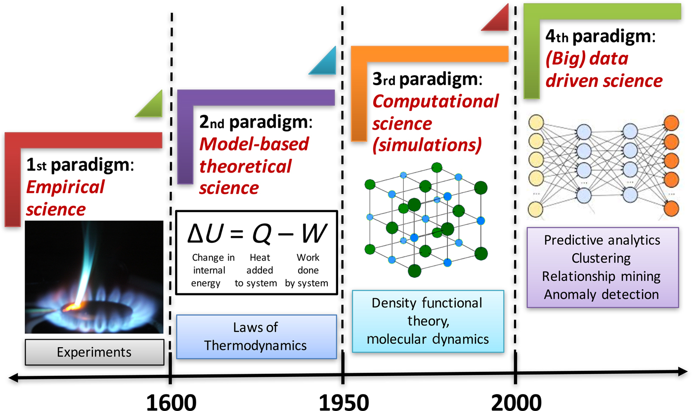
In this era of big data, we are being bombarded with huge volumes of data from a variety of different sources (experiments and simulations) at a staggering velocity in practically all fields of science and engineering, and materials science is no exception. This has led to the emergence of the fourth paradigm of science, which is data-driven science, and builds upon the big data created by the first three paradigms of science (experiment, theory, and simulation). Advanced techniques for data-driven analytics are needed to analyze these data in ways that can help extract meaningful information and knowledge from them, and thus contribute to accelerating materials discovery and realize the vision of Materials Genome Initiative (MGI).[1] The fourth paradigm of science utilizes scalable machine learning (ML) and data mining techniques to extract actionable insights from such big data and inform materials design efforts at various levels. Figure 1 depicts the four paradigms of science.[Reference Agrawal and Choudhary2]
The four paradigms of science in the context of materials. Historically, science has been largely empirical or observational, which is known today as the experimental branch of science. When calculus was invented in the 17th century, it became possible to describe natural phenomena in the form of mathematical equations, marking the beginning of second paradigm of science, which is model-based theoretical science. With time, these equations became larger and more complex, and it was only in the 20th century when computers were invented that such larger and complex theoretical models (system of equations) became solvable, enabling large-scale simulations of real-world phenomena, which is the third paradigm of science. The last two decades have seen an explosive growth in the generation of data from the first three paradigms, which has far out-stripped our capacity to make sense of it. All this collected data can serve as a valuable resource for learning and augmenting the knowledge from first three paradigms, and has led to the emergence of the fourth paradigm of science, which is (big) data-driven science (reproduced from Ref. Reference Agrawal and Choudhary2 under CC-BY license).
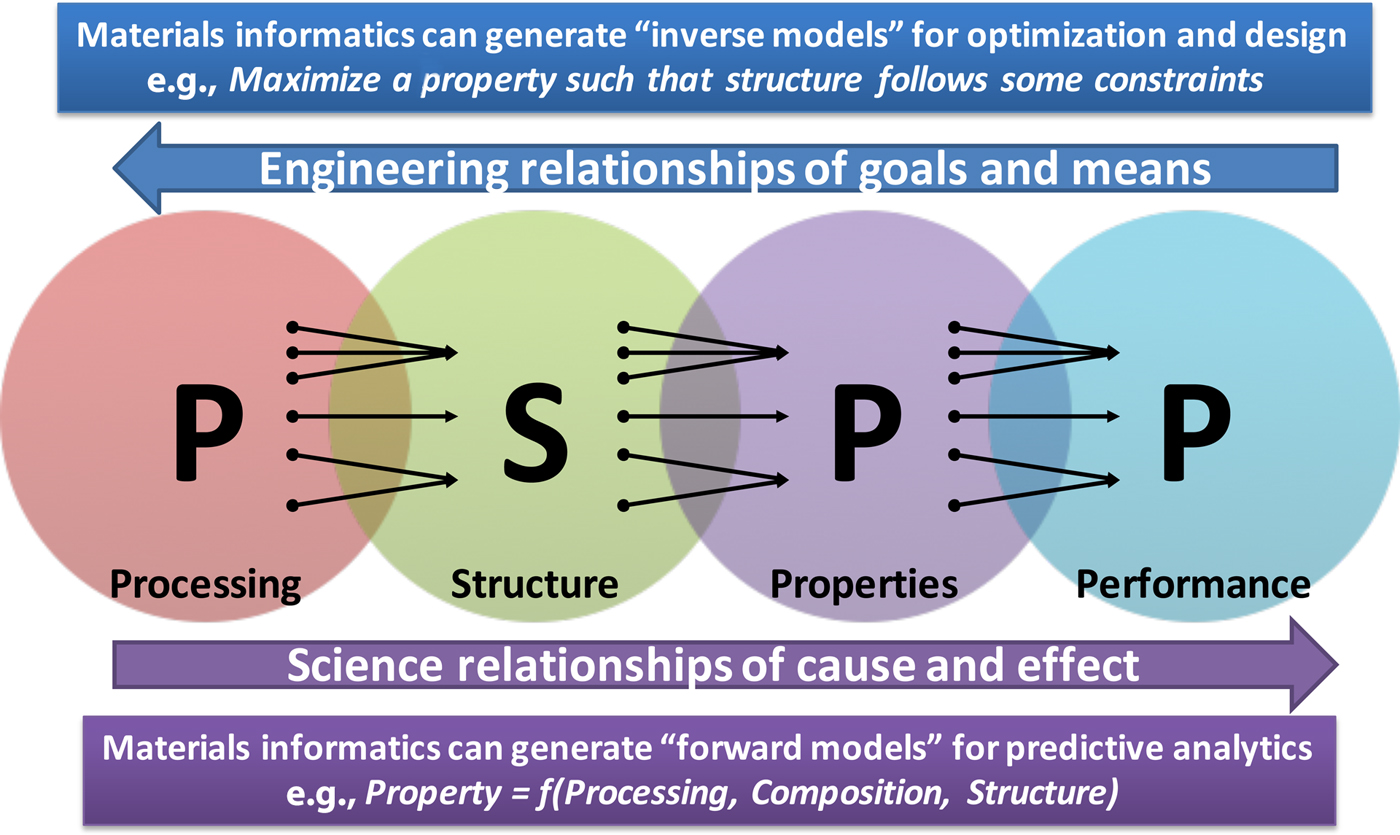
Materials science and engineering researchers rely on experiments and simulations to try to understand the processing–structure–property–performance (PSPP) relationships,[Reference Agrawal and Choudhary2,Reference Olson3] which are far from being well-understood. In fact, almost everything in materials science depends on these PSPP relationships, where the cause–effect relationships of science go from left to right, and the goals–means relationships of engineering go from right to left. In order to discover and design new improved materials with desired properties, we need to better understand this complex system of PSPP relationships. Figure 2 depicts these PSPP relationships of materials science and engineering.[Reference Agrawal and Choudhary2]
The PSPP relationships of materials science and engineering, where science flows from left-to-right, and engineering flows from right-to-left. Interestingly, each relationship from left to right is many-to-one. For example, many different processing routes can possibly result in the same structure, and along similar lines, it is also possible that the same property is achieved by multiple material structures. Materials informatics approaches can help decipher these relationships via fast and accurate forward models, which in turn can also help to realize the more difficult inverse models of materials discovery and design (reproduced from Ref. Reference Agrawal and Choudhary2 under CC-BY license).
The scalable data-driven techniques[Reference Papalexakis, Faloutsos and Sidiropoulos4–Reference Xie, Chen, Palsetia, Trajcevski, Agrawal and Choudhary8] of the fourth paradigm of science have found numerous applications in a lot of diverse fields such as marketing and commerce,[Reference Fan, Lau and Zhao9,Reference Xu, Frankwick and Ramirez10] healthcare,[Reference Agrawal, Choudhary, Sobolev, Levy and Goring11,Reference Belle, Thiagarajan, Soroushmehr, Navidi, Beard and Najarian12] climate science,[Reference Ganguly, Kodra, Agrawal, Banerjee, Boriah, Chatterjee, Chatterjee, Choudhary, Das, Faghmous, Ganguli, Ghosh, Hayhoe, Hays, Hendrix, Fu, Kawale, Kumar, Kumar, Liao, Liess, Mawalagedara, Mithal, Oglesby, Salvi, Snyder, Steinhaeuser, Wang and Wuebbles13,Reference Karpatne and Kumar14] bioinformatics,[Reference Kashyap, Ahmed, Hoque, Roy and Bhattacharyya15,Reference Zhang, Misra, Agrawal, Patwary, Liao, Qin and Choudhary16] social media,[Reference Bello-Orgaz, Jung and Camacho17,Reference Lee, Agrawal and Choudhary18] materials science,[Reference Rajan19,Reference Ramprasad, Batra, Pilania, Mannodi-Kanakkithodi and Kim20] and cosmology,[Reference Kremer, Stensbo-Smidt, Gieseke, Pedersen and Igel21,Reference Rangel, Li, Habib, Peterka, Agrawal, Liao and Choudhary22] among many others. In particular, over the last few years, deep learning[Reference LeCun, Bengio and Hinton23] has emerged as a game-changing technique within the arena of data-driven analytics due to its revolutionary success in several traditionally hard artificial intelligence (AI) applications. Deep learning techniques are also increasingly being used for materials informatics applications with remarkable success, which we refer to as deep materials informatics.
In this paper, we discuss some of the recent advances in deep materials informatics for exploring PSPP linkages in materials, after a brief introduction to the basics of deep learning, and its challenges and opportunities. Illustrative examples of deep materials informatics that we review in this paper include learning the chemistry of materials using only elemental composition,[Reference Jha, Ward, Paul, Liao, Choudhary, Wolverton and Agrawal24] structure-aware property prediction,[Reference Xie and Grossman25,Reference Ye, Chen, Wang, Chu and Ong26] crystal structure prediction,[Reference Ryan, Lengyel and Shatruk27] learning multiscale homogenization[Reference Yang, Yabansu, Al-Bahrani, Liao, Choudhary, Kalidindi and Agrawal28,Reference Cecen, Dai, Yabansu, Kalidindi and Song29] and localization[Reference Yang, Yabansu, Jha, Liao, Choudhary, Kalidindi and Agrawal30] linkages in high-contrast composites, structure characterization[Reference Liu, Agrawal, Liao, Graef and Choudhary31,Reference Jha, Singh, Al-Bahrani, Liao, Choudhary, Graef and Agrawal32] and quantification,[Reference DeCost, Lei, Francis and Holm33,Reference Patton, Johnston, Young, Schuman, March, Potok, Rose, Lim, Karnowski., Ziatdinov and Kalinin34] and microstructure reconstruction[Reference Li, Zhang, Zhao, Burkhart, Brinson and Chen35] and design.[Reference Yang, Li, Brinson, Choudhary, Chen and Agrawal36] We also discuss the future outlook and envisioned impact of deep learning in materials science before summarizing and concluding the paper.
Deep learning
Deep learning[Reference LeCun, Bengio and Hinton23] refers to a family of techniques in AI and ML, and is essentially a rediscovery of neural networks that were algorithmically conceptualized back in the 1980s.[Reference Rumelhart, Hinton and Williams37,Reference Rumelhart, Hinton and Williams38] The availability of big data and big compute in recent years have allowed these networks to grow deeper (hence the name deep learning) and realize their promise to be universal approximators[Reference Hornik39] capable learning and representing a wide variety of non-linear functions. Deep learning has indeed emerged as a very powerful method to automate the extraction of useful information from big data, and has enabled ground-breaking advances in numerous fields, such as computer vision[Reference Krizhevsky, Sutskever, Hinton, Pereira, Burges, Bottou and Weinberger40,Reference He, Zhang, Ren and Sun41] and speech recognition.[Reference Hinton, Deng, Yu, Dahl, Mohamed, Jaitly, Senior, Vanhoucke, Nguyen, Sainath and Kingsbury42,Reference Deng, Hinton and Kingsbury43] In the rest of this section, we will briefly describe the unique advantages and limitations of deep learning, followed by the key components of a deep neural network, and finally a few different types of networks being used for deep materials informatics.
Deep learning: advantages and limitations
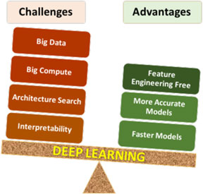
Deep learning has certain unique characteristics compared to traditional ML techniques, which are crucial for determining whether or not deep learning should be used for a given problem. These characteristics (both advantages and challenges) are depicted in Fig. 3, and described below. There are three primary advantages of deep learning compared to traditional ML methods:
• Deep learning is largely feature-engineering-free: This is perhaps the biggest advantage of deep learning. It is well-known that the efficacy of a ML model depends a lot on how the data are represented for the ML algorithm to learn patterns from. Usually for a scientific or engineering application, a good representation would often entail careful feature engineering, which may require extensive domain knowledge as well as significant manual and intuitive effort to come up with the appropriate attributes. In contrast, deep learning is capable of automatically extracting the relevant features from the training data in a hierarchical fashion, thereby eliminating or at least reducing the effort for feature engineering. Not only does this help save the manual effort of having to come up with attributes, but also opens up opportunities to identify new, non-intuitive features in a truly data-driven manner that might help discover new insights.
• Deep learning is generally more accurate with big data: Any data-driven ML model is expected to become more accurate with increasing training data, but the accuracy does saturate at some point, after which additional training data does not provide significant accuracy gains. It has been found that although for small data, traditional ML based models are more accurate than deep learning based models, they saturate much sooner, so deep learning based models are usually more accurate when big data is available. This is because of the higher learning capacity possessed by deep neural networks with multiple hidden layers.
• Deep learning can produce faster predictions: Although training neural networks is computationally expensive, it is only a one-time cost. Once trained properly, they are capable of making very fast predictions.
Pros and cons of deep learning. As with any technique, there are advantages and challenges of using deep learning that need to be considered carefully for successful application.

The above-described advantages of deep learning clearly give it an edge over traditional ML techniques, but it nonetheless has some characteristics that make its application challenging in some cases. There are four major challenges in applying deep learning:
• Deep learning requires big data: In many cases, the biggest limiting factor for applying deep learning is lack of sufficient training data. As discussed before, deep learning requires big data in general. Although big, curated, and labeled datasets do exist for several problems like image classification,[Reference Deng, Dong, Socher, Li, Li and Fei-Fei44] they are still a rarity in many scientific and engineering fields, such as materials science.[Reference Agrawal and Choudhary2]
• Deep learning requires big compute: Training deep learning based models is compute-intensive and can take a long time with big data, even on the latest computing hardware. Parallelization of neural network training algorithms is an active area of research.[Reference Lee, Jha, Agrawal, Choudhary and Liao45,Reference Mnih, Badia, Mirza, Graves, Lillicrap, Harley, Silver and Kavukcuoglu46]
• Deep learning network architecture search: Since a neural network is essentially a network of interconnected neurons, there are unlimited possibilities of network architectures. Although there are some general guidelines for choosing an architecture for a given problem based on prior successful designs, there are no formal methods to identify the optimal architecture for a given task, and it is an open research problem.[Reference Patton, Johnston, Young, Schuman, March, Potok, Rose, Lim, Karnowski., Ziatdinov and Kalinin34]
• Model interpretability: Deep learning based models are generally viewed as black-box models due to being highly complex. Although researchers have tried with some success to systematically study the workings of the neural network, in general they are not as readily interpretable as some of the traditional statistical models like linear regression.[Reference Lou, Caruana and Gehrke47]
Deep learning: key components and concepts
Artificial neural networks (ANNs) are inspired by biological neural networks in our brains. The fundamental computing unit of ANNs is a neuron, which takes multiple inputs, and outputs a possibly non-linear function (called the activation function) of the weighted sum of its inputs. Several activation functions are commonly used, such as sigmoid, linear, rectified linear unit (ReLU), leaky ReLU, etc. Figure 4 illustrates a fully-connected ANN, also known as multilayer perceptron (MLP), and the ReLU activation function. A deep learning network is an ANN with two or more hidden layers. The manner in which the neurons are connected amongst themselves determines the architecture of the network. The edges or interconnections between neurons have weights, which are learned during neural network training with the goal of making the ANN output as close as possible to the ground truth, which is technically referred to as minimizing the loss function. The training process involves making a forward pass of the input data through the ANN to get predictions, calculating the errors or loss, and subsequently back-propagating them through the network to update the weights of the interconnections via gradient descent in order to try to make the outputs more accurate. A single pass of the entire training data is called an epoch, and it is repeated iteratively till the weights converge. Usually when the data are large, the forward passes are done with small subsets of the training data (called mini-batches), so an epoch would comprise of multiple iterations of mini-batches. The inputs of a neural network are generally normalized to have zero mean and unit standard deviation, and the same concept is sometimes applied to the input of hidden layers as well (called batch normalization) to improve the stability of ANNs. Another useful and interesting concept in ANNs is that of dropouts, where some neurons are randomly turned off during a particular forward or backward pass. It is a regularization technique for reducing overfitting, and also turns out to be a remarkably efficient approximation to multi-model averaging.[Reference Srivastava, Hinton, Krizhevsky, Sutskever and Salakhutdinov48]
A fully-connected deep ANN with four inputs, one output, and five hidden layers with varying number of neurons (left). The ReLU activation function (right).

Convolutional neural networks
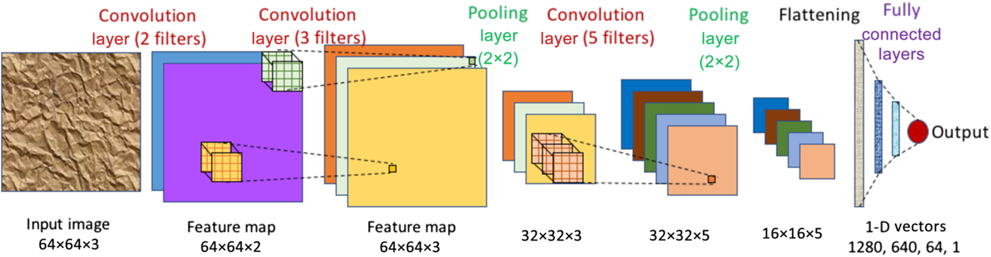
A convolutional neural network (CNN) is a special kind of deep learning network which is designed to be used on spatial data such as images, and consists of three types of hidden layers. It is designed to appropriately capture spatially correlated features in images using convolutional layers. A convolutional layer consists of multiple kernels or filters with trainable weights or parameters. Each filter is applied across the input image as a convolving window to extract abstract features in the form of feature maps, which are used as inputs for the next layer. Pooling layers are usually used after one or more convolutional layers to reduce the size of the feature maps by subsampling them in both spatial dimensions using an aggregation function (such as max, min, avg), which also reduces the number of parameters and helps in controlling overfitting. After several blocks of convolutional and pooling layers, the outputs are flattened to a long one-dimensional (1-D) vector, to be used as input to one or more fully connected layers to finally give the CNN prediction, which could either be a probability distribution (for classification problems) or a single numerical value (for regression problems). Two-dimensional (2-D) CNNs that work with 2-D input matrices (images) as depicted in Fig. 5 are the most common type of CNNs, but there are other variants such as 1-D and three-dimensional (3-D) CNNs that take 1-D vectors and 3-D matrices respectively as input, and graph CNNs[Reference Kipf and Welling49,Reference Zhou, Cui, Zhang, Yang, Liu and Sun50] that can work with graphs (a collection of nodes and edges) as input.
A CNN with three convolution layers, two pooling layers, and three fully connected layers. It takes a 64 × 64 RGB image (i.e., three channels) as input. The first convolution layer has two filters resulting in a feature map with two channels (depicted in purple and blue). The second convolution layer has three filters, thereby producing a feature map with three channels. It is then followed by a 2 × 2 pooling layer, which reduces the dimensionality of the feature map from 64 × 64 to 32 × 32. This is followed by another convolution layer of five filters, and another pooling layer to reduce feature map dimension to 16 × 16 (five channels). Next, the feature map is flattened to get a 1-D vector of 16 × 16 × 5 = 1280 values, which is fed into three fully connected layers of 640, 64, and one neuron(s) respectively, finally producing the output value.
Generative adversarial networks
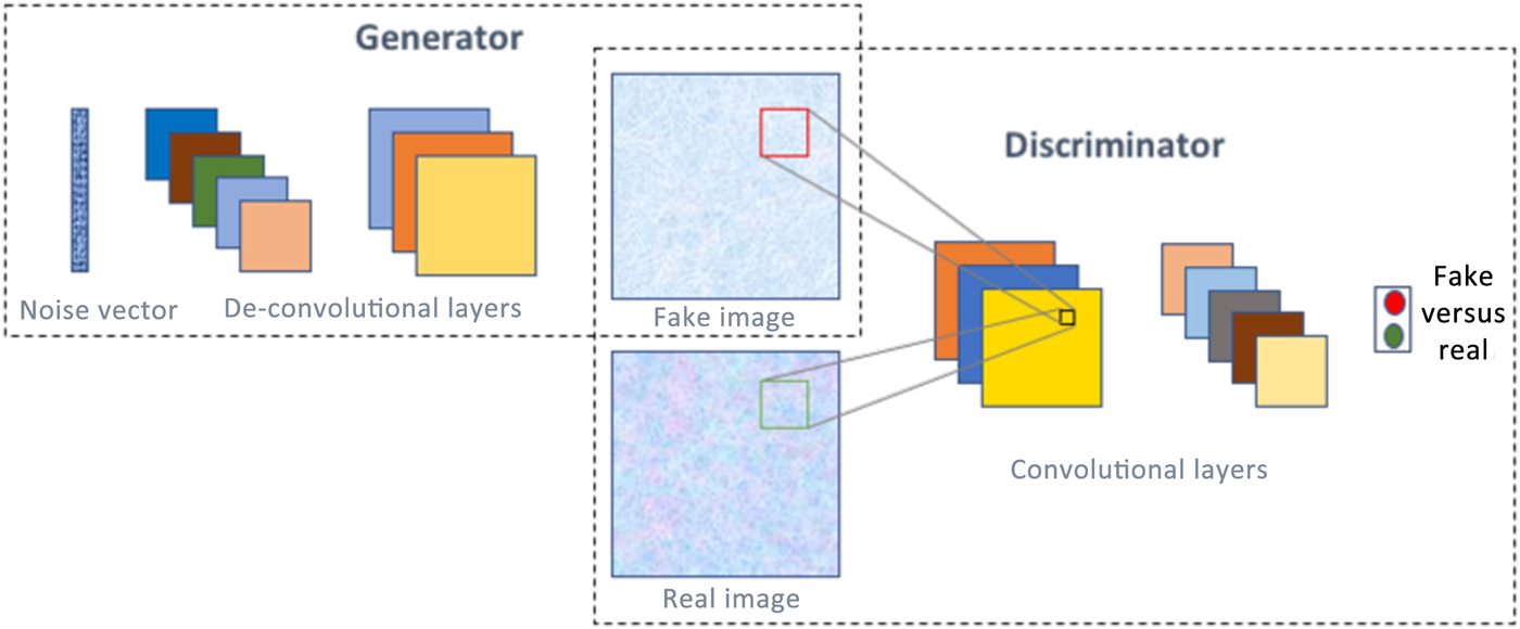
A generative adversarial network (GAN)[Reference Goodfellow, Pouget-Abadie, Mirza, Xu, Warde-Farley, Ozair, Courville and Bengio51] is one of the most interesting type of deep learning network architectures in recent years, and has originated from game theory. It consists of not one but two neural networks that are trained simultaneously in a competitive fashion. One of the networks is called a generator, which is essentially an inverse convolutional network, taking in a random noise vector and up-sampling it to a fake image. Then there is a discriminator, which is a standard convolutional network, taking an image as input and down-sampling it to produce a probability distribution, to classify the input image as fake or real. Figure 6 illustrates the concept of GANs. A common analogy often used to describe GANs is that the generator can be thought of like a criminal trying to produce fake currency, and the discriminator like the police whose aim is to identify the currency as fake or real. As the two networks are trained together, they make each other progressively strong till they achieve the Nash equilibrium.[Reference Osborne and Rubinstein52] It is not surprising that GANs have found numerous interesting applications in image analysis, such as high-resolution image synthesis,[Reference Wang, Liu, Zhu, Tao, Kautz and Catanzaro53] text to image synthesis,[Reference Zhang, Xu, Li, Zhang, Wang, Huang and Metaxas54] image editing,[Reference Perarnau, van de Weijer, Raducanu and Álvarez55] blending,[Reference Wu, Zheng, Zhang and Huang56] inpainting,[Reference Pathak, Krahenbuhl, Donahue, Darrell and Efros57] etc., as well as in non-image domains, like music generation.[Reference Yang, Chou and Yang58]
A GAN consists of two neural networks—generator and discriminator, and with proper training, is capable of generating realistic images/data from noise.
Illustrative deep materials informatics
We now review some recent applications of deep learning in materials science for understanding PSPP relationships, both in terms of forward models and inverse models. These examples also illustrate the previously discussed unique characteristics of deep learning in the context of materials.
Learning the chemistry of materials from only elemental composition
As described before, one of the biggest advantages of deep learning is that it is feature-engineering-free and capable of directly working on raw inputs without the need of manually engineered features to incorporate domain knowledge. Jha et al.[Reference Jha, Ward, Paul, Liao, Choudhary, Wolverton and Agrawal24] recently demonstrated the same on materials composition data, by developing a new deep learning network called ElemNet, which takes only the elemental composition of a crystalline compound as input and predicts its formation enthalpy. They used a large simulation dataset of density functional theory (DFT) calculations from the Open Quantum Materials Database (OQMD) for building the deep learning model. The dataset consisted of 275,759 compounds and their corresponding formation enthalpies. Previous studies[Reference Meredig, Agrawal, Kirklin, Saal, Doak, Thompson, Zhang, Choudhary and Wolverton59–Reference Agrawal, Meredig, Wolverton and Choudhary61] on formation enthalpy prediction have relied on the use of hundreds of composition-derived features called physical attributes (such as average atomic number, average electronegativity, and so on) for constructing ML models, in a bid to provide known chemistry knowledge to the model. However, such a feature extraction step depends heavily on human intuition and domain expertise. Moreover, it may not always be possible to do this step for all problems, as the necessary domain knowledge may not be available or it may be difficult to transform it into quantitative features for ML algorithms to use. Therefore, the authors in Ref. Reference Jha, Ward, Paul, Liao, Choudhary, Wolverton and Agrawal24 purposely did not provide any domain knowledge to the model in order to investigate how well a model can perform in such a situation. They explored different depths of the fully-connected neural network until 24 layers. The accuracy of the deep learning model rapidly improved until 17 layers, after which it plateaued. ElemNet, the best-performing 17-layer neural network was found to outperform traditional ML algorithms, both with and without physical attributes. The Random Forest model (the best performing traditional ML technique) gave a mean absolute error (MAE) of 0.157 eV/atom using only elemental compositions as features, and 0.071 eV/atom using composition-derived physical attributes as input. In contrast, ElemNet, which only uses elemental compositions as input, was found to give a significantly lower MAE of 0.055 eV/atom. Modeling experiments with different training set size revealed that ElemNet performs better than Random Forest model (even with physical attributes) for all training set sizes greater than 4000, thereby serving as another testimony of the superior performance of deep learning models on large datasets. In terms of computation time, ElemNet took significantly longer for training (about 7 h on a GPU for a training set of ~250,000 compounds), but was much faster in terms of prediction time (9.28 s on a CPU and 0.08 s on a GPU for a test set of ~25,000 compounds). ElemNet was also evaluated with two specially designed training-test splits (withholding the Ti–O binary system and Na–Fe–Mn–O quaternary system, respectively) to find that it can also predict the phase diagrams (convex hulls) for unseen materials systems.
In order to understand why ElemNet was performing well, the authors also studied the representation learned by the network, to try to interpret the model, by analyzing the activations produced within the network at different layers for specific inputs provided to the model. It was found that ElemNet self-learns some interesting chemistry like groups (element similarity) in the early layers, and charge balance (element interaction) in later layers of the network, although no periodic table information was provided to the model during training. For example, the activations of first and second layers produced by group-I elements such as Li, Na, K, Rb, and Cs were all clustered together in a straight line (in that order), when projected in a 2-D space using principal component analysis (PCA). Similarly, when binary combinations of group-I/II and group-VI/VII elements were passed through the model, it was found that the charge balanced and unbalanced compositions tend to cluster separately in the eighth layer of ElemNet. This is consistent with other applications of deep learning, for example, on images, where the initial layers learn simple features such as edges and corners, and then use those features to learn more complex ones such as shapes in next few layers, and so on. The high accuracy and speed of ElemNet allowed the authors to perform combinatorial screening on about half-a-billion compounds in the quaternary space. They found a number of systems with at least one new potential stable compound, including several new compounds that were not in the OQMD but exist in the Inorganic Crystal Structure Database (ICSD), thereby confirming their stability.
Crystal structure aware property prediction
Although composition-based models can be quite accurate as illustrated in the previous example, the role of structure is critical in materials, as allotropes and polymorphs can have contrasting properties with the same composition. Hence, it is also important to build structure-aware models for materials property prediction. There exist a number of studies that use different set of attributes to represent the structure information[Reference Schütt, Glawe, Brockherde, Sanna, Müller and Gross62–Reference Ward, Liu, Krishna, Hegde, Agrawal, Choudhary and Wolverton65] for the ML algorithms to build predictive models. Recently, deep learning has also been applied directly on the crystal structure, as discussed next.
Xie and Grossman[Reference Xie and Grossman25] developed a crystal graph CNN framework to directly learn material properties from the connection of atoms in the crystal. Their approach first represents the crystal structure by a crystal graph where nodes represent the atoms in the unit cell and edges represent the bonds between the atoms, and then builds a CNN on the graph with convolutional layers, fully connected layers, and pooling layers, to automatically extract optimum representations for modeling the target properties. Their database consisted of 46,744 materials from the Materials Project[Reference Jain, Ong, Hautier, Chen, Richards, Dacek, Cholia, Gunter, Skinner, Ceder and Persson66] covering 87 elements, 7 lattice systems, and 216 space groups. A simple convolution function using a shared weight matrix for all neighbors of an atom resulted in a MAE of 0.108 eV/atom for formation energy prediction. However, it neglected the differences of interaction strength between neighbors, so they designed a new convolution function taking into account the interaction strength in the form of a learned weight matrix, which gave a much improved MAE of 0.039 eV/atom. The same framework was subsequently applied to other DFT-computed properties from the Materials Project, such as absolute energy, band gap, Fermi energy, bulk moduli, shear moduli, and Poisson ratio. Apart from impressive model accuracies obtained by deep-learning models, their framework also provided for model interpretability to some degree, by removing the fully-connected hidden layers after atom feature vector extraction and directly performing a linear pooling to predict the property. This allowed the model to learn the contribution of different local chemical environments for each atom to the target property, at the cost of a dip in accuracy [MAE of 0.130 eV/atom on 3787 test perovskites (ABX3) with the interpretable model versus 0.099 eV/atom with the full model]. The empirical rules generalized from the perovskites study were found to be consistent with known knowledge, and a combinatorial search leveraging the learned chemical insights led to the discovery of several new perovskites.
Of course, another way to take structure information into account is to build structure-specific models, i.e., only train on materials of a specific structure class. For example, Ye et al.[Reference Ye, Chen, Wang, Chu and Ong26] recently demonstrated that ANNs utilizing just two descriptors (the Pauling electronegativity and ionic radii of constituent elements) can predict DFT formation energies of C3A2D3O12 garnets and ABO3 perovskites with low MAEs of 0.007–0.010 eV/atom and 0.020–0.034 eV/atom, respectively. For mixed garnets, i.e., garnets with more than one type of species in the C, A, and D sites, the authors derived an averaging scheme to model complete cation disorder and a binary encoding scheme to account for the effect of orderings, with minimal loss in accuracy.
Crystal structure prediction
One of the grand challenges in materials science has been crystal structure prediction,[Reference Oganov67] much like protein structure prediction in bioinformatics.[Reference Dill, Ozcan, Weikl, Chodera and Voelz68] The problem of crystal structure prediction for a given composition can be decomposed into two primary sub-problems: generation of candidate structures, followed by subsequent evaluation of those structures to identify the most likely one(s). Typically, structure generation approaches use evolutionary algorithms with random initialization,[Reference Bail69,Reference Glass, Oganov and Hansen70] which are then evaluated by quantum mechanical methods.[Reference Gautier, Zhang, Hu, Yu, Lin, Sunde, Chon, Poeppelmeier and Zunger71] Ryan et al.[Reference Ryan, Lengyel and Shatruk27] recently presented a remarkable application of deep learning for crystal structure prediction, in particular for crystal structure evaluation. They reformulated the crystal structure prediction problem into that of predicting the likelihoods of individual atomic sites in the structure, thereby approximating the likelihood of a crystal structure to exist by the product of the likelihoods for each element to reside on a specific atomic site.
To calculate the element likelihood for a given atomic site (element prediction problem), the authors in Ref. Reference Ryan, Lengyel and Shatruk27 designed a deep neural network using training data from the ICSD and Crystallographic Open Database, with 704,334 unique crystallographic sites in 51,723 crystal structures. The input representation of atomic sites for model training consisted of multiple perspectives of normalized atomic fingerprints, to capture the local topology around each unique atomic site. This input representation provided several useful characteristics such as translational invariance, fixed dimensionality, and retention of 3-D information, and allowed the model to learn structural topologies rather than crystal structures with specific scale. The deep neural network itself consisted of three subnetworks. First, a 42-layer convolutional variational autoencoder was used to allow the model to learn its own representation of the atomic fingerprints, which reduced the 3072-dimensional atomic fingerprints to 64-dimensional latent representations. Then, these latent representations were fed into a five-layer sigmoid classifier to predict what combinations of elements were likely to form specific structural topologies. Finally, the resulting likelihoods from the sigmoid classifier were fed into a five-layer auxiliary softmax classifier with batch normalization and 118 output neurons to predict what specific element corresponded to the input, thereby formulating the element prediction problem as a 118-class classification problem. The average error rate on the test set (20% of entire atomic fingerprints data) was found to be 31%, which is quite impressive for a 118-class problem. Interestingly, most of the errors made by the model were found to be chemically reasonable (e.g., within blocks of 3d and 4f elements). Further, a t-SNE (t-distributed stochastic neighbor embedding, an iterative method for mapping high-dimensional data onto a 2-D or 3-D projection for visualization[Reference Van der Maaten and Hinton72]) embedding of the sigmoid classifier weights for the elements revealed groupings similar to those in the periodic table. It is indeed quite remarkable that the deep learning model was able to learn periodic trends and chemical similarities not explicitly provided to the model while training, simply by learning from raw structural information, just like the ElemNet model[Reference Jha, Ward, Paul, Liao, Choudhary, Wolverton and Agrawal24] did from raw composition information.
Returning to the crystal structure prediction problem, the work in Ref. Reference Ryan, Lengyel and Shatruk27 used the set of known structure types as the starting point for generating new crystal structures, and the above-described deep learning model for crystal structure evaluation. The unique crystallographic sites in 51,723 known structures were used as structural templates for the generator to produce new crystal structures by combinatorial substitution across the series of all elements, thus leading to 623,380 binary and 2,703,834 ternary candidate crystal structures. Coupling this structure generation approach with deep learning based structure evaluation allowed the authors to perform crystal structure prediction. The performance of the structure prediction was evaluated on a holdout test set of 5845 crystal structures, and it was found that the model is able to predict the correct structure as the top-ranked candidate 27% of the time, and the correct structure is within top-10 predicted structures 59% of the time, which is an underestimate of its true performance due to the presence of isostructural crystal structures in the candidate list. The authors also presented a case study of Mn–Ge and Li–Mn–Ge systems, and reported new unique chemical compositions in these systems, with corresponding predicted structure templates. The key takeaway from this work is the demonstrated potential of deep learning models to self-learn chemistry knowledge from purely geometric and topological data, and its application to the important problem of crystal structure prediction.
Multiscale homogenization and localization linkages in high-contrast composites
While the previous examples used deep learning on composition and crystal structure data, in this subsection, we look at some examples of the application of deep learning on 3-D microstructure data of two-phase composites for understanding structure–property linkages, which are often required to be understood across different length scales. In such multi-scale modeling, homogenization refers to transfer of microstructure information from lower length scales to higher length scales, e.g., prediction of macroscale property given its microstructure information. Localization deals with transfer of salient microstructure information from a higher length scale to lower length scale. For example, when a material is subject to a macroscopic loading condition (like imposed stress or strain rate), localization refers to the manner in which the load gets distributed at the microscale for a given microstructure. Both homogenization and localization linkages are modeled together by numerical approaches like microscale finite element simulations or iterative methods employing Green's functions. In recent years, materials knowledge systems (MKS)[Reference Brough, Wheeler and Kalidindi73] have emerged as a promising approach for understanding localization relationships, which utilize calibrated Green's function-based kernels in a non-iterative series solution, as well as ML-based methods that rely on feature engineering to capture the local neighborhood of the microstructure.
Yang et al.[Reference Yang, Yabansu, Al-Bahrani, Liao, Choudhary, Kalidindi and Agrawal28] present a feature-engineering-free deep learning based homogenization solution for predicting macroscale effective stiffness in two-phase composites of contrast 50. Contrast refers to the relative dissimilarity in the property of the two constituent phases. In this case, it is the ratio of the Young's moduli of the two phases. The dataset consisted of 8550 simulated 3-D microstructures of size 51 × 51 × 51, also referred to as microscale volume elements (MVEs). Recall from PSPP relationships that structure is the cause and property is the effect. Therefore for a given loading condition, the macroscale property (in this case effective stiffness) depends on the microstructure. The effective stiffness was calculated using micromechanical finite element simulations with periodic boundary conditions. In order to learn homogenization linkages using deep leaning, the authors used 3-D CNNs to map microstructure information to effective stiffness. The best deep-learning network was identified as a 14-layer model with five convolution blocks (consisting of a convolution layer followed by a pooling layer) stacked together, and subsequently followed by two fully connected layers. In total, this network had about 3.8 million trainable parameters. The accuracy of the deep-learning model [MAE of 1.04 GPa (3.10%)] was found to be significantly better than simple physics-based approaches or rule of mixtures method [MAE of 15.68 GPa (46.66%)] and sophisticated physics-inspired data science approaches that utilize PCA on two-point statistics as input features for regression[Reference Gupta, Cecen, Goyal, Singh and Kalidindi74] [MAE of 2.28 GPa (6.79%)]. Another recent related work[Reference Cecen, Dai, Yabansu, Kalidindi and Song29] on using deep learning for homogenization has demonstrated that the filters/kernels learned by the CNN during training can be interpreted as microstructure features that the model learns to be influential for improving the macroscale property of interest. This can be extremely valuable for solving the inverse problem of design exploration, thereby closing the loop and informing materials design.
Yang et al.[Reference Yang, Yabansu, Jha, Liao, Choudhary, Kalidindi and Agrawal30] present a novel feature-engineering-free approach for localization using deep learning. They used two datasets of contrast-10 (2500 MVEs) and contrast-50 (3000 MVEs) of size 21 × 21 × 21 with varying volume fraction and periodic boundary conditions, and were split into training, validation, and test sets. Since each voxel is a data point for the localization problem, a 3-D neighborhood of size 11 × 11 × 11 around the focal voxel was used to represent the focal voxel. Although 3-D CNNs could be used for this problem as well, the dataset here is almost four orders of magnitude larger, and since 3-D CNNs are much more computationally expensive, the authors in Ref. Reference Yang, Yabansu, Jha, Liao, Choudhary, Kalidindi and Agrawal30 designed a neat workaround to be able to use 2-D CNNs for localization. They accomplished this by treating the 3-D image of size 11 × 11 × 11 as 11 channels of a 2-D images of size 11 × 11, perpendicular to the maximum principal strain direction. The best performing CNN architecture for this problem consisted of six layers, with two convolution layers and two fully-connected layers. The accuracy of the deep learning model was compared against the MKS method,[Reference Brough, Wheeler and Kalidindi73] and two ML-based methods called single-agent method[Reference Liu, Yabansu, Agrawal, Kalidindi and Choudhary75] and multi-agent method,[Reference Liu, Yabansu, Yang, Choudhary, Kalidindi and Agrawal76] which is essentially a hierarchical application of the single-agent method. On contrast-10 dataset, the MKS method resulted in a mean absolute strain error (MASE) of 10.86%, while the single-agent and multi-agent methods gave a MASE of 13.02% and 8.04%, respectively. In contrast, the deep learning CNN model gave a significantly lower MASE of 3.07%. For contrast-50, the MKS method gave a MASE of 26.46% as compared to just 5.71% by the deep learning model. A closer look at what the CNN learned revealed that the influence of different level neighbors decreases with increasing level of neighbors, which is consistent with known domain knowledge.
Microstructure characterization and quantification
Materials characterization broadly refers to learning structural information of a given material, and is one of the fundamental processes to further our understanding of materials.[Reference Leng77] Advances in materials characterization technologies at different time and length scales such as numerous kinds of microscopy, spectroscopy, and macroscopic testing has led to a proliferation in materials image data, which has motivated the use of deep learning to solve this inverse characterization problem.
Electron backscatter diffraction (EBSD) is one of the many materials imaging tools to determine crystal orientation of crystalline materials, which can be represented by the three Euler angles 〈φ1,Φ,φ2〉. The inverse structure characterization problem of determining the orientation angles given an EBSD pattern is called EBSD indexing. The commercially available method for EBSD indexing is the Hough transform based method,[Reference Schwartz, Kumar, Adams and Field78] which is quite effective in general, but susceptible to the presence of noise in the patterns. In recent years, a new method called dictionary based indexing[Reference Chen, Park, Wei, Newstadt, Jackson, Simmons, De Graef and Hero79] has been developed, which is essentially a nearest neighbor search approach, where the output angles correspond to the orientation angles of the closest EBSD pattern present in a pre-computed high-resolution dictionary. This method is very robust to noise, but computationally very expensive, as the input EBSD pattern needs to be compared to every pattern in the dictionary. Liu et al.[Reference Liu, Agrawal, Liao, Graef and Choudhary31] presented the first application of deep learning (CNNs) for indexing EBSD patterns using a dictionary of 333,227 simulated EBSD patterns (60 × 60 gray scale images), out of which 300,000 were used from training and rest for testing. Although the CNN results were found to be more accurate than the dictionary method, this work had two significant limitations. First of all, not using the entire dictionary for training is suboptimal and thus would underestimate the accuracy of both dictionary method and the CNN. Second, they created three separate models for the three Euler angles thereby treating them independent, which is not true as they are actually partial representations of the same orientation. Therefore, rather than individually minimizing the difference between the three actual and predicted Euler angles, the model should really be trying to minimize the one angle between the corresponding orientations, which is technically called disorientation. Jha et al.[Reference Jha, Singh, Al-Bahrani, Liao, Choudhary, Graef and Agrawal32] recently presented a new deep learning solution for EBSD indexing overcoming these limitations. They used two dictionaries consisting of a total of 374,852 EBSD patterns for training the model, and an independent set of 1000 simulated EBSD patterns with known orientations for testing. Here the authors optimized for mean disorientation error between the predicted and true orientations as the loss function for CNN training, which posed two challenges. First, the disorientation metric is computationally expensive, as one needs to compute 24 × 24 symmetrically equivalent orientation pairs. Second, the presence of crystal symmetries introduces degeneracies in the orientation space resulting in discontinuities in the gradients of the disorientation loss function, thereby rendering it inappropriate for optimization using stochastic gradient descent. To overcome the above challenges, the authors designed a differentiable approximation to the original disorientation function by building a computational tensor graph in TensorFlow,[Reference Abadi, Barham, Chen, Chen, Davis, Dean, Devin, Ghemawat, Irving, Isard and Kudlur80] leveraging its auto-differentiation support. The CNN consisted of eight convolution layers, two pooling layers, and five fully connected layers, making it a 17-layer network with about 200 million parameters. In terms of accuracy, the deep learning model outperformed dictionary-based indexing by 16% (mean disorientation of 0.548° versus 0.652° for the dictionary method).
DeCost et al.[Reference DeCost, Lei, Francis and Holm33] present a deep learning solution for quantitative microstructure analysis for ultrahigh carbon steel, by building models for two microstructure segmentation tasks: (i) semantic segmentation of steel micrographs into four regions (grain boundary carbide, spheroidized particle matrix, particle-free grain boundary denuded zone, and Widmanstätten cementite); and (ii) segmenting cementite particles within the spheroidized particle matrix. Unlike image classification, segmentation is a pixel-level task, and thus the CNN needs to produce a latent representation of each pixel instead of the entire image. The authors used the PixelNet[Reference Bansal, Chen, Russell, Gupta and Ramanan81] architecture for this purpose, where each pixel is represented by the concatenation of its representations in each convolutional layer by applying bilinear interpolation to intermediate feature maps and getting a hypercolumn feature vector for each pixel. Subsequently a MLP is used to map the hypercolumn pixel features to the corresponding target, i.e., segmentation classes. They used the pretrained VGG16 network[Reference Simonyan and Zisserman82] (trained on the ImageNet database[Reference Deng, Dong, Socher, Li, Li and Fei-Fei44]) for the convolutional layers of PixelNet, and trained the MLP layers from scratch, with batch normalization, dropout, weight decay regularization, and data augmentation. Two kinds of loss functions were evaluated: the standard cross-entropy classification loss and focal loss, which extends the cross-entropy classification loss function with a modulating factor and scaling parameter to account for the model confidence and class imbalance respectively. The dataset consisted of 24 ultrahigh carbon steel micrographs at a resolution of 645 × 484. Sixfold cross validation was used to evaluate the models in terms of segmentation accuracy as well as comparison of actual and predicted distributions of particle size and denuded zone widths. The segmentation model with focal loss function was found to be the most accurate for spheroidite and particle segmentation. However, most of the predicted particle size distributions were found to differ from those from human-annotated micrographs, as the model failed to identify small particles with radii smaller than 5 pixels, indicating the need of higher quality input for training. This work nonetheless demonstrated the efficacy of deep learning for microstructural segmentation and quantitative analysis for complex microstructures at a high level of abstraction.
Patton et al.[Reference Patton, Johnston, Young, Schuman, March, Potok, Rose, Lim, Karnowski., Ziatdinov and Kalinin34] recently presented a 167-petaflop projected (152.5-petaflop measured; petaflop is a unit of computing speed, equaling 1015 floating point operations per second) deep learning system called MENNDL to automate raw electron microscopy image based atomic defect identification and analysis on a supercomputer using 4200 nodes (with six GPUs per node). It intelligently generates and evaluates millions of deep neural networks with varying architectures and hyperparameters using a scalable, parallel, asynchronous, genetic algorithm augmented with a support vector machine to automatically find the best performing network, all in a matter of hours, which is much faster than a human expert can do. The resulting deep learning network also allowed the authors to create a library of defects, map chemical transformation pathways at the atomic level, including detailed transition probabilities, and explore subtle distortions in local atomic environment around the defects of interest. Further, it also lets the computer automatically choose the best region in the sample to make a measurement or perform atomic manipulations without human supervision, which is a critical step toward enabling an autonomous (self-driving) microscope.
Microstructure reconstruction and design
Reconstruction of the structure of a disordered heterogeneous material using limited structural information about the original system remains an important problem in modeling of heterogeneous materials.[Reference Piasecki83] Li et al.[Reference Li, Zhang, Zhao, Burkhart, Brinson and Chen35] developed a deep transfer learning based approach for reconstructing statistically equivalent microstructures from arbitrary material systems based on a single given microstructure. In their approach, the input microstructure with k labeled material phases is first encoded to a three-channel (RGB) representation to make it amenable to be used as an input to a pruned version of a pretrained CNN called VGG19.[Reference Simonyan and Zisserman82] At the same time, another randomly initialized RGB image (which would iteratively be updated to become the encoded microstructure reconstruction) is also passed through the pruned VGG19 network. The loss function to be minimized is the difference of Gram-matrix (a measure of texture of a given image)[Reference Gatys, Ecker and Bethge84] between the activations of the original and reconstructed microstructure, summed over selected convolutional layers of the pruned VGG19. During neural network training, typically the gradient of the loss function with respect to the network weights is calculated to iteratively optimize the weights and refine the model. But here, the weights of the network are kept constant, and the pixel values of the randomly initialized reconstructed microstructure are the variables to be optimized. Therefore, the gradient of the loss with respect to each pixel in the reconstructed microstructure is computed via backpropagation, and is subsequently fed into a nonlinear optimization algorithm to iteratively update the pixel values of the microstructure reconstruction, till it converges. The converged reconstruction at this point is still encoded though, and thus is subsequently decoded using k-means clustering to separate the pixels into k groups, where k is the number of material phases in the original microstructure. Since this process pipeline ending with k-means clustering does not enforce retention of the original volume fraction (relative ratio of different phases), it is possible that the volume fractions are slightly different from the original microstructure, which is not desirable. Therefore, the authors employed another post-processing step using simulated annealing to switch the phase label of some of the boundary pixels in order to match the phase volume fractions in original and reconstructed microstructures. The approach was successfully tested on a wide variety of structural morphologies (carbonate, polymer composites, sandstone, ceramics, a block copolymer, a metallic alloy, and three-phase rubber composites) and found to outperform other approaches (decision tree based synthesis,[Reference Bostanabad, Bui, Xie, Apley and Chen85] Gaussian random field (GRF),[Reference Grigoriu86] two point correlation,[Reference Liu, Greene, Chen, Dikin and Liu87] and physical descriptor[Reference Xu, Dikin, Burkhart and Chen88]) in four out of the five material systems.
Microstructure design is an important inverse problem for materials design. One of the key tasks for this purpose is to identify suitable microstructure representations that could be used for design. Yang and Li et al.[Reference Yang, Li, Brinson, Choudhary, Chen and Agrawal36] have recently developed a deep adversarial learning methodology for an end-to-end solution for low-dimensional and non-linear embedding of microstructures for microstructural materials design using GANs. GAN-based microstructure design is able to capture complex, non-linear microstructure characteristics owing to the large model capacity offered by deep learning networks, and learn the mapping between latent variables (input noise vector) and microstructures. Subsequently, the low-dimensional latent variables can serve as design variables. The GAN was trained on 5000 synthetic microstructure images of size 128 × 128 created using the GRF method. The GAN generator (discriminator) consisted of five layers with the size of feature maps doubling (halving) along each dimension for each layer. Therefore, the 128 × 128 images are reduced by a factor of 25 (=32) in each dimension, thus converting it to a 4 × 4 latent variable matrix, or 16-dimensional latent variable vector. Once the GAN was trained, it was able to generate new microstructure images simply by randomly sampling the latent variable vector and passing it through the generator. Not only did the generated microstructure images visually looked similar to the real images, but they were also confirmed to be similar in terms of two-point correlation function and lineal-path correlation function. To evaluate the capability of the trained GAN for microstructure optimization and design, it was coupled with a Bayesian optimization approach to search for the optimal microstructure representation (in terms of latent variable vector) along with rigorous coupled wave analysis to simulate the optical absorption performance of a given microstructure. Results indicated that the optical performance of the GAN-generated microstructures (even without Bayesian optimization) was 4.8% better than that of randomly sampled microstructures, and the same for the optimized microstructure (with Bayesian optimization) was 17.2% better than that of randomly sampled microstructures, thereby verifying the effectiveness of the design optimization framework. In addition to the demonstrated capability of generating realistic microstructure images as well as microstructure optimization and design, the authors report a couple of other desirable features of the developed GAN model. These include the ability of the trained generator to generate arbitrary sized microstructures by changing the size of the latent variables (scalability), and the ability of the discriminator to be used as a pre-trained model for developing structure–property prediction models (transferability).
Future outlook and impact
Deep learning is a fast growing field that has attracted a lot of attention, which has led to fascinating algorithmic advances being introduced at an incredible pace. In this section, we discuss some other crucial facets of deep learning in context of materials informatics, which are expected to shape the growing impact of data-driven approaches in materials science.
Other types of deep learning networks
In addition to the different kinds of deep learning neural networks (such as MLPs, CNNs, and GANs) we have seen so far in this paper, there are several others that are capable of analyzing other forms of data. For example, recurrent neural networks are designed to work with sequence data (also known as temporal or time-series data) of varying lengths, with most popular applications in speech recognition[Reference Miao, Gowayyed and Metze89] natural language processing,[Reference Xie, Daga, Cheng, Zhang, Agrawal and Choudhary90] as well as some recent applications in materials informatics.[Reference Mozaffar, Paul, Al-Bahrani, Wolff, Choudhary, Agrawal, Ehmann and Cao91,Reference Paul, Jha, Al-Bahrani, Liao, Choudhary and Agrawal92] A relatively new class of deep learning is called geometric deep learning which is capable of dealing with non-Euclidean data, such as graphs with nodes and edges, where standard deep learning kernels like convolution are not well-defined. Due to its ability to work with graph data, it has found applications in quantum chemistry,[Reference Gilmer, Schoenholz, Riley, Vinyals and Dahl93,Reference Schütt, Sauceda, Kindermans, Tkatchenko and Müller94] in particular for analyzing data from molecular dynamics simulations.
Transfer learning
As discussed before, deep learning generally requires big data, but transfer learning can enable the application of deep learning for problems where big data are not available, by transferring knowledge from a deep learning model built on big data for a different but related problem, to build a new model on the smaller data for the problem at hand. Transfer learning is expected to be very useful for materials informatics, since most of the materials datasets are usually small in size, compared to the big data available in some other domains such as social media, bioinformatics, cosmology, etc. It is widely used in image classification, where pre-trained deep learning models built on ImageNet[Reference Deng, Dong, Socher, Li, Li and Fei-Fei44] (a large image database of more than 14 million labeled images) like VGG[Reference Simonyan and Zisserman82] are used to extract key features from small image datasets and build ML models.[Reference Gopalakrishnan, Khaitan, Choudhary and Agrawal95]
Uncertainty quantification and active learning
Uncertainty quantification (UQ) for predictive analytics is an important topic, and one that is expected to gain more and more attention in materials informatics in the coming years. It essentially means the ability to identify calibrated uncertainty estimates for the predictions made by a ML model, by trying to capture the expected variance in the response within a specified confidence interval. A commonly used methodology for UQ that has also been used in materials informatics is an ensemble data mining approach,[Reference Agrawal and Choudhary96] where multiple predictive models are constructed for the same task by using different techniques on the same data and/or the same technique on different subsets of the training data, and the final prediction is calculated as a function of the individual predictions, such as mean. In such cases, the uncertainty can be quantified using the standard deviation of the individual predictions, possibly combined with the model prediction error. Deep learning models provide an alternate way to do the same without having to build multiple models. Recall that dropout during neural network training randomly shuts down some neurons, thereby helping the model to become more generalizable, and it can also approximate model ensembling.[Reference Srivastava, Hinton, Krizhevsky, Sutskever and Salakhutdinov48] While making predictions from the model (testing phase), dropout again randomly drops some neurons, so the same input to the model would generate (slightly) different predictions every time the model is run with dropout. The resulting set of predictions can be used to calculate uncertainty estimates, just like with ensemble learning models or using more sophisticated methods.[Reference Gal, Hron and Kendall97]
UQ also holds the key for active learning and reinforcement learning, where the predictive model is used to recommend which new unlabeled inputs should be labeled next (based on their predicted value and associated uncertainties) in order to have the greatest improvement in the accuracy of the model, or to take a suitable action in a given situation that would maximize the reward. Interestingly, active learning has a direct application for data-driven materials discovery, where based on a given experimental or simulation materials dataset, it can recommend which experiment or simulation should be done next to further improve the predictive models. The new improved models can again be used with active learning to identify the next best experiment or simulation, and so on. In this way, it can significantly reduce the number of experiments needed to discover the optimal material with a target property of interest, thereby accelerating the inverse models of materials discovery and design.
Model interpretability
The issue of model interpretability has always been a crucial one for many applications such as financial modeling, autonomous driving, as well as materials engineering, where the cost of a false positive can be immeasurably large, making it critical to ensure that the model is not just quantitatively accurate but is in fact learning from the correct features and learning things that make sense, at least not learning something known to be false. Lipton[Reference Lipton98] presents one of the first attempts toward a comprehensive taxonomy of the desiderata and methods in interpretability research, and identifies transparency to humans and post-hoc explanations as two primary and competing notions of interpretability. The transparency aspect of interpretability relates to understanding how the model works, in terms of the training algorithm, the intuitive significance of individual model inputs and parameters, and the overall working of the trained model. There is usually a trade-off between model transparency and model complexity, and Lipton[Reference Lipton98] suggests that no model is intrinsically interpretable, e.g., even linear models with highly engineered and complex inputs, deep decision trees, ensembles, etc. could be considered less transparent than comparatively compact neural networks with raw or lightly processed inputs. Post-hoc explanations, on the other hand, relates to understanding what the model has learned. Since deep learning models learn rich representations, they are especially useful for post-hoc interpretability, which can be done via visualization techniques such as t-SNE[Reference Van der Maaten and Hinton72] to visualize its latent representations in 2-D, or saliency maps[Reference Simonyan, Vedaldi and Zisserman99] to identify the regions of the input that influence the output the most. Further, for a given test example, its low-dimensional latent representation (e.g., activations of the hidden layers) can be used to identify its k-nearest neighbors in the training set, so as to explain the decisions of the model by reporting other similar examples,[Reference Lipton98] and provide another way of interpreting deep learning models. Several other methods and guidelines to understand deep leaning networks are available.[Reference Montavon, Samek and Müller100]
Potential long-term impact
Materials are fundamental building blocks of a civilization. The advancement of our society relies on the development of better, safer, more efficient, cost-effective, and environment-friendly materials. Deep materials informatics approaches have the potential to be game changing for materials scientists and industry, by assisting researchers to navigate through the practically infinite space of possible materials and identify a few most promising ones, which can then be evaluated with appropriate simulations and experiments, thereby significantly reducing costs and accelerating the discovery and deployment of advanced materials. Deep materials informatics therefore provides remarkable promise to accelerate the discovery and design of next generation materials in a cost-effective manner, and thus realize the vision of MGI. Illustrative real-world applications that could potentially be impacted by deep materials informatics include construction, automobile, clean energy, aerospace, healthcare, transportation, and so on.
Summary and conclusion
Materials informatics is a rapidly emerging field but still in its early stages, similar to what bioinformatics was about 20 years ago,[Reference Agrawal and Choudhary2] and this is even more true for deep materials informatics, which is the application of deep learning in materials science. In this paper, we discussed some of the recent advances in deep materials informatics on a variety of materials data like elemental composition, crystal structure, and 2-D/3-D microstructures images. The fundamental concepts in deep learning, its advantages, challenges, types of popular deep learning networks, and future outlook and impact of deep materials informatics were also discussed. The increasingly availability of materials databases and big data in general, along with groundbreaking advances in data science and deep learning approaches offer a lot of promise to revolutionize materials property prediction, discovery, design, and deployment of next-generation materials.
Acknowledgments
The authors gratefully acknowledge partial support from the following grants: NIST awards 70NANB19H005, 70NANB14H012; AFOSR award FA9550-12-1-0458; NSF award CCF-1409601; DOE awards DE-SC0007456, DE-SC0014330. The authors would also like to thank all the collaborators and contributors of the papers that were reviewed in this paper.


 Open access