
 c=∞
c=∞ 1
1





1. Introduction
The kinetic equation, which describes the interaction of matter with photons, is the radiative transfer equation. The radiative transfer equation can be written including absorption-emission processes and scattering processes in a rather general setting as
 \begin{equation} \frac {1}{c}\partial _t I_\nu (t,x,n)+n\cdot \nabla _x I_\nu (t,x,n)=\alpha _\nu ^e-\alpha _\nu ^aI_\nu (t,x,n)+\alpha _\nu ^s\left (\displaystyle\int _{\mathbb{S}^2} K(n,n')I_\nu (t,x,n')\;dn'-I_\nu (t,x,n)\right ). \end{equation}
We denote by $ I_\nu (t,x,n)$
the radiation intensity, that is, the distribution of energy of photons moving at time
$ I_\nu (t,x,n)$
the radiation intensity, that is, the distribution of energy of photons moving at time $ t\gt 0$
, at position
$ t\gt 0$
, at position $ x\in \Omega \subset {\mathbb{R}}^3$
and in direction
$ x\in \Omega \subset {\mathbb{R}}^3$
and in direction $ n\in {\mathbb{S}^2}$
with frequency
$ n\in {\mathbb{S}^2}$
with frequency $ \nu \gt 0$
. Moreover,
$ \nu \gt 0$
. Moreover, $ c$
is the speed of light in the medium that will be assumed to be constant. The parameters
$ c$
is the speed of light in the medium that will be assumed to be constant. The parameters $ \alpha ^e$
,
$ \alpha ^e$
, $ \alpha ^a$
and
$ \alpha ^a$
and $ \alpha ^s$
are, respectively, the emission, absorption and scattering coefficients. These are functions that can depend on the frequency
$ \alpha ^s$
are, respectively, the emission, absorption and scattering coefficients. These are functions that can depend on the frequency $ \nu$
, on the position
$ \nu$
, on the position $ x$
or, in the case of local thermal equilibrium, on the local temperature
$ x$
or, in the case of local thermal equilibrium, on the local temperature $ T(x)$
. The function
$ T(x)$
. The function $ K$
is the scattering kernel. It can be considered as the probability rate of a photon to be deflected from an incident direction
$ K$
is the scattering kernel. It can be considered as the probability rate of a photon to be deflected from an incident direction $ n'\in {\mathbb{S}^2}$
to a new direction
$ n'\in {\mathbb{S}^2}$
to a new direction $ n\in {\mathbb{S}^2}$
. The scattering kernel
$ n\in {\mathbb{S}^2}$
. The scattering kernel $ K$
can also be assumed to depend on the frequency
$ K$
can also be assumed to depend on the frequency $ \nu \in {\mathbb{R}}_+$
. However, in this paper, we omit the dependence on
$ \nu \in {\mathbb{R}}_+$
. However, in this paper, we omit the dependence on $ \nu$
in order to simplify the notation. Notice that all the results that we will present in this paper also hold in the case where
$ \nu$
in order to simplify the notation. Notice that all the results that we will present in this paper also hold in the case where $ K$
is a function of
$ K$
is a function of $ \nu$
.
$ \nu$
.
In this paper, we will study the heat transfer by means of radiation under some assumptions. First of all, we consider only the case of local thermal equilibrium in which the temperature $ T(t,x)$
is well-defined at any point
$ T(t,x)$
is well-defined at any point $ x\in \Omega$
and for any time
$ x\in \Omega$
and for any time $ t\gt 0$
. This is not necessarily the case in situations where the microscopic processes driving the system towards equilibrium are slow. Such problems arise in applications to astrophysics (cf. [Reference Oxenius45]). Under this assumption, the emission coefficient takes a particular form. Indeed, it is given by
$ t\gt 0$
. This is not necessarily the case in situations where the microscopic processes driving the system towards equilibrium are slow. Such problems arise in applications to astrophysics (cf. [Reference Oxenius45]). Under this assumption, the emission coefficient takes a particular form. Indeed, it is given by $ \alpha _\nu ^e= \alpha _\nu ^a B_\nu (T(t,x))$
, where
$ \alpha _\nu ^e= \alpha _\nu ^a B_\nu (T(t,x))$
, where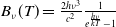 $ B_\nu (T)= \frac {2h\nu ^3}{c^2}\frac {1}{e^{\frac {h\nu }{kT}}-1}$
is the Planck distribution of a black body. We assume also that the considered material is isotropic without a preferred direction of scattering. Hence, the scattering kernel
$ B_\nu (T)= \frac {2h\nu ^3}{c^2}\frac {1}{e^{\frac {h\nu }{kT}}-1}$
is the Planck distribution of a black body. We assume also that the considered material is isotropic without a preferred direction of scattering. Hence, the scattering kernel $ K$
is invariant under rotations.
$ K$
is invariant under rotations.
We couple the radiative transfer equation with the energy balance equation
 \begin{equation} C\partial _t T(t,x)+\frac {1}{c}\partial _t\left (\displaystyle\int _0^\infty d\nu \displaystyle\int _{\mathbb{S}^2} dn\;I_\nu (t,x,n)\right )+\textrm {div}\left (\displaystyle\int _0^\infty d\nu \displaystyle\int _{\mathbb{S}^2} dn\;nI_\nu (t,x,n)\right )=0, \end{equation}
where $ C\gt 0$
is the volumetric heat capacity of the material. The combined system (1.1) and (1.2) allows to determine the temperature of the system at any point when the heat is transferred only by means of radiation. Notice that in (1.2), we are not considering other heat transport processes such as conduction or convection. After a suitable time rescaling, we can assume
$ C\gt 0$
is the volumetric heat capacity of the material. The combined system (1.1) and (1.2) allows to determine the temperature of the system at any point when the heat is transferred only by means of radiation. Notice that in (1.2), we are not considering other heat transport processes such as conduction or convection. After a suitable time rescaling, we can assume $ C=1$
. As a boundary condition, we consider a source of radiation placed at infinity. Mathematically, we impose
$ C=1$
. As a boundary condition, we consider a source of radiation placed at infinity. Mathematically, we impose
 \begin{equation} I_\nu (t,x,n)=g_\nu (t,n)\;\;\text{ if } x\in {\partial \Omega }\text{ and }n\cdot n_x\lt 0, \end{equation}
where $ n_x\in {\mathbb{S}^2}$
is the outer normal to the boundary at point
$ n_x\in {\mathbb{S}^2}$
is the outer normal to the boundary at point $ x$
. However, we could consider a more general setting with the incoming boundary profile
$ x$
. However, we could consider a more general setting with the incoming boundary profile $ g_\nu (t,x,n)$
depending also on
$ g_\nu (t,x,n)$
depending also on $ x\in {\partial \Omega }$
.
$ x\in {\partial \Omega }$
.
In this paper we, will consider both the time-dependent and the stationary cases. Assuming $ \Omega \subset {\mathbb{R}}^3$
bounded and convex and as initial values the bounded functions
$ \Omega \subset {\mathbb{R}}^3$
bounded and convex and as initial values the bounded functions $ I_0(x,n,\nu )$
and
$ I_0(x,n,\nu )$
and $ T_0(x)$
, we consider the following initial-boundary value problem
$ T_0(x)$
, we consider the following initial-boundary value problem
 \begin{equation} \!\!\begin{cases} \dfrac {1}{c}\partial _tI_\nu (t,x,n)+n\cdot \nabla _x I_\nu (t,x,n)=\alpha _\nu ^a(x)\left (B_\nu (T(t,x))-I_\nu (t,x,n)\right )\\[5pt] {\phantom {nel mezzo del cammin di nostra}}+\alpha _\nu ^s(x)\left (\displaystyle\int _{\mathbb{S}^2} K(n,n')I_\nu (t,x,n')\;dn'-I_\nu (t,x,n)\right )& x\in \Omega ,n\in {\mathbb{S}^2},t\gt 0\\[5pt] \partial _tT+\dfrac {1}{c}\partial _t \left (\displaystyle\int _0^\infty d\nu \displaystyle\int _{\mathbb{S}^2} dn \;I_\nu (t,n,x)\right ) +\textrm {div}\left (\displaystyle\int _0^\infty d\nu \displaystyle\int _{\mathbb{S}^2} dn \;nI_\nu (t,n,x)\right )=0& x\in \Omega ,n\in {\mathbb{S}^2},t\gt 0\\[5pt] I_\nu (0,x,n)=I_0(x,n,\nu )& x\in \Omega ,n\in {\mathbb{S}^2}\\[5pt] T(0,x)=T_0(x)& x\in \Omega \\[5pt] I_\nu (t,n,x)=g_\nu (t,n)& x\in {\partial \Omega },n\cdot n_x\lt 0,t\gt 0 \end{cases} \end{equation}
and the following stationary boundary value problem
 \begin{equation} \begin{cases} n\cdot \nabla _x I_\nu (x,n)=\alpha _\nu ^a(x)\left (B_\nu (T(x))-I_\nu (x,n)\right )\\[5pt] {\phantom {nel mezzo del cammin di nostra}}+\alpha _\nu ^s(x)\left (\displaystyle\int _{\mathbb{S}^2} K(n,n')I_\nu (x,n')\;dn'-I_\nu (x,n)\right )& x\in \Omega ,n\in {\mathbb{S}^2}\\[5pt] \textrm {div}\left (\displaystyle\int _0^\infty d\nu \displaystyle\int _{\mathbb{S}^2} dn \;nI_\nu (n,x)\right )=0& x\in \Omega ,n\in {\mathbb{S}^2}\\[5pt] I_\nu (n,x)=g_\nu (n)& x\in {\partial \Omega },n\cdot n_x\lt 0. \end{cases} \end{equation}
Problems like (1.4) and (1.5) or similar equations related to radiative transfer are often studied in the framework of the so-called diffusion approximation (see [Reference Mihalas and Mihalas42, Reference Zel’dovich, Raizer, Hayes and Probstein58]). This approximation is valid when the mean free path of the photons is much smaller than the macroscopic size of the system. However, the mean free path of the photons can be small because either the scattering mean free path or the absorption mean free path is smaller than the size of the system. The main consequence of that is that, depending on the ratio between the different mean free paths, the radiation intensity can be approximated by the Planck distribution, that is, $ B_\nu (T)$
, or it cannot be. The first case is denoted as equilibrium diffusion approximation, while the second one is referred to as non-equilibrium diffusion approximation. These concepts have been extensively discussed in the physical literature on radiation (cf. [Reference Mihalas and Mihalas42, Reference Zel’dovich, Raizer, Hayes and Probstein58]). The goal of this paper is to obtain a precise mathematical characterization of these concepts, specifically to derive an accurate mathematical condition for the validity of the equilibrium diffusion approximation and to determine the regions where the equilibrium or non-equilibrium diffusion approximation holds for the specific problems (1.4) and (1.5). To this end, we will use perturbative methods and matched asymptotic expansions in order to study different scaling limits for the scattering and absorption mean free paths.
$ B_\nu (T)$
, or it cannot be. The first case is denoted as equilibrium diffusion approximation, while the second one is referred to as non-equilibrium diffusion approximation. These concepts have been extensively discussed in the physical literature on radiation (cf. [Reference Mihalas and Mihalas42, Reference Zel’dovich, Raizer, Hayes and Probstein58]). The goal of this paper is to obtain a precise mathematical characterization of these concepts, specifically to derive an accurate mathematical condition for the validity of the equilibrium diffusion approximation and to determine the regions where the equilibrium or non-equilibrium diffusion approximation holds for the specific problems (1.4) and (1.5). To this end, we will use perturbative methods and matched asymptotic expansions in order to study different scaling limits for the scattering and absorption mean free paths.
1.1. Scaling lengths and results
We study the solutions of the time-dependent and stationary radiative transfer equations (1.4) and (1.5) under different scaling limits, and we obtain suitable problems satisfied by the limit of the solutions of the original problems. For these problems, we will obtain either the equilibrium or the non-equilibrium diffusion approximation. To this end, we start defining some characteristic lengths.
We consider a convex domain $ \Omega \subset {\mathbb{R}}^3$
with diameter of order
$ \Omega \subset {\mathbb{R}}^3$
with diameter of order $ 1$
and such that the size of the domain is comparable in all directions of the space. Moreover, the characteristic macroscopic length
$ 1$
and such that the size of the domain is comparable in all directions of the space. Moreover, the characteristic macroscopic length $ L$
is assumed to be
$ L$
is assumed to be $ L=1$
. We remark that many of the results obtained in this paper are also valid in a non-convex domain. However, in non-convex domains, we should also take into account the consequences of incoming radiation into cavities, an issue that we will not consider in this paper (see [Reference Jang and Velázquez30] for more details).
$ L=1$
. We remark that many of the results obtained in this paper are also valid in a non-convex domain. However, in non-convex domains, we should also take into account the consequences of incoming radiation into cavities, an issue that we will not consider in this paper (see [Reference Jang and Velázquez30] for more details).
We will replace the absorption coefficient $ \alpha _\nu ^a(x)$
by
$ \alpha _\nu ^a(x)$
by
 \begin{equation} \frac {\alpha _\nu ^a(x)}{\ell _A} \end{equation}
and the scattering coefficient $ \alpha _\nu ^s(x)$
by
$ \alpha _\nu ^s(x)$
by
 \begin{equation} \frac {\alpha _\nu ^s(x)}{\ell _S}, \end{equation}
where now $ \alpha _\nu ^a(x)=\mathcal{O}(1)$
and
$ \alpha _\nu ^a(x)=\mathcal{O}(1)$
and $ \alpha _\nu ^s(x)=\mathcal{O}(1)$
are bounded by a constant of order one in both variables. We denote by
$ \alpha _\nu ^s(x)=\mathcal{O}(1)$
are bounded by a constant of order one in both variables. We denote by $ \ell _A$
the absorption length and by
$ \ell _A$
the absorption length and by $ \ell _S$
the scattering length. These are also the mean free paths of the absorption/emission processes and the scattering processes, respectively. In some physical applications, it is convenient to assume
$ \ell _S$
the scattering length. These are also the mean free paths of the absorption/emission processes and the scattering processes, respectively. In some physical applications, it is convenient to assume $ \alpha _\nu ^a(x)$
or
$ \alpha _\nu ^a(x)$
or $ \alpha _\nu ^s(x)$
to tend to zero for large or small frequencies
$ \alpha _\nu ^s(x)$
to tend to zero for large or small frequencies $ \nu$
. The exact dependence of these functions on
$ \nu$
. The exact dependence of these functions on $ \nu$
will be made after. Roughly speaking, we have to assume that they have to decay not too fast in order to obtain that some integrals arising in the analysis are convergent.
$ \nu$
will be made after. Roughly speaking, we have to assume that they have to decay not too fast in order to obtain that some integrals arising in the analysis are convergent.
In many technological applications, it can be assumed that $ \alpha _\nu ^s\ll \alpha _\nu ^a$
(cf. [Reference Zel’dovich, Raizer, Hayes and Probstein58]). However, there are also applications where the scattering plays a more important role than the absorption/emission process. This is the case, for example, in the analysis of planetary atmospheres (see [Reference Friedlander20, Reference Oxenius45]).
$ \alpha _\nu ^s\ll \alpha _\nu ^a$
(cf. [Reference Zel’dovich, Raizer, Hayes and Probstein58]). However, there are also applications where the scattering plays a more important role than the absorption/emission process. This is the case, for example, in the analysis of planetary atmospheres (see [Reference Friedlander20, Reference Oxenius45]).
Another important scaling length that we should consider is the Milne length, which is given by the minimum between absorption and scattering length,
 \begin{equation} \ell _M=\min \{\ell _A,\ell _S\}. \end{equation}
The Milne length can be considered to be the effective mean free path of the whole radiative process. The key feature of the Milne length is that at distances of order $ \ell _M$
to the boundary, the radiation intensity becomes isotropic, that is, independent of the direction
$ \ell _M$
to the boundary, the radiation intensity becomes isotropic, that is, independent of the direction $ n\in {\mathbb{S}^2}$
. Since we are interested in the diffusion approximation, we assume in the rest of this paper
$ n\in {\mathbb{S}^2}$
. Since we are interested in the diffusion approximation, we assume in the rest of this paper $ \ell _M\ll L= 1$
.
$ \ell _M\ll L= 1$
.
Another length that plays a crucial role in the analysis of this paper is the quantity that we will denote as thermalization length, which is the geometrical mean of the absorption and the Milne length
 \begin{equation} \ell _T=\sqrt {\ell _A\ell _M}. \end{equation}
The thermalization length is the characteristic distance from the boundary at which the radiation intensity $ I_\nu$
approaches the Planck equilibrium distribution of the temperature.
$ I_\nu$
approaches the Planck equilibrium distribution of the temperature.
We now replace in (1.4) and (1.5) the absorption and scattering coefficients with the expressions in (1.6) and (1.7). The changes in the temperature take place in times of order
 \begin{equation*} \tau _{\mathit{h}}=\frac {\ell _A}{\min \{\ell _T^2,1\}}\gg 1, \end{equation*}
which will be denoted as the heat parameter. Therefore, in order to obtain an equation that changes in times $ t$
of order
$ t$
of order $ 1$
, we will replace
$ 1$
, we will replace $ t$
by
$ t$
by $ \tau _{\mathit{h}}t$
. Notice that, after this change of variable, the changes of times
$ \tau _{\mathit{h}}t$
. Notice that, after this change of variable, the changes of times $ t$
of order
$ t$
of order $ 1$
are associated with relevant changes of the temperature of order
$ 1$
are associated with relevant changes of the temperature of order $ 1$
. We will use this notation throughout the paper; that is, we will denote by
$ 1$
. We will use this notation throughout the paper; that is, we will denote by $ t$
the time after the change of variable. Hence, (1.4) writes using
$ t$
the time after the change of variable. Hence, (1.4) writes using $ L=1$
 \begin{equation} \begin{cases} \dfrac {1}{c}\partial _tI_\nu (t,x,n)+\tau _{\mathit{h}} n\cdot \nabla _x I_\nu (t,x,n)=\dfrac {\alpha _\nu ^a(x)\tau _{\mathit{h}}}{\ell _A}\left (B_\nu (T(t,x))-I_\nu (t,x,n)\right )\\[5pt] {\phantom {nel mezzo del cammin di no}}+\dfrac {\alpha _\nu ^s(x)\tau _{\mathit{h}}}{\ell _S}\left (\displaystyle\int _{\mathbb{S}^2} K(n,n')I_\nu (t,x,n')\;dn'-I_\nu (t,x,n)\right )& x\in \Omega ,n\in {\mathbb{S}^2},t\gt 0\\[5pt] \partial _tT+\dfrac {1}{c}\partial _t \left (\displaystyle\int _0^\infty d\nu \displaystyle\int _{\mathbb{S}^2} dn \;I_\nu (t,n,x)\right )& \\[5pt] \phantom{spacespacespace} \qquad\qquad+\tau _{\mathit{h}}\textrm {div}\left (\displaystyle\int _0^\infty d\nu \displaystyle\int _{\mathbb{S}^2} dn \;nI_\nu (t,n,x)\right ) =0 & x\in \Omega ,n\in {\mathbb{S}^2},t\gt 0\\[5pt] I_\nu (0,x,n)=I_0(x,n,\nu )& x\in \Omega ,n\in {\mathbb{S}^2}\\[5pt] T(0,x)=T_0(x)& x\in \Omega \\[5pt] I_\nu (t,n,x)=g_\nu (t,n)&x\in {\partial \Omega },n\cdot n_x\lt 0,t\gt 0. \end{cases} \end{equation}
We will also consider the case where the speed of light is infinite, that is, $ c= \infty$
. This approximation is justified if the characteristic time for the temperature to change is much smaller than the time required for the light to cross the domain. In this case, the equation will be
$ c= \infty$
. This approximation is justified if the characteristic time for the temperature to change is much smaller than the time required for the light to cross the domain. In this case, the equation will be
 \begin{equation} \begin{cases} n\cdot \nabla _x I_\nu (t,x,n)=\dfrac {\alpha _\nu ^a(x)}{\ell _A}\left (B_\nu (T(t,x))-I_\nu (t,x,n)\right )\\[5pt] {\phantom {nel mezzo del cammin}}+\dfrac {\alpha _\nu ^s(x)}{\ell _S}\left (\displaystyle\int _{\mathbb{S}^2} K(n,n')I_\nu (t,x,n')\;dn'-I_\nu (t,x,n)\right )& x\in \Omega ,n\in {\mathbb{S}^2},t\gt 0\\[5pt] \partial _tT+\tau _{\mathit{h}}\textrm {div}\left (\displaystyle\int _0^\infty d\nu \displaystyle\int _{\mathbb{S}^2} dn \;nI_\nu (t,n,x)\right )=0& x\in \Omega ,n\in {\mathbb{S}^2},t\gt 0\\[5pt] T(0,x)=T_0(x)& x\in \Omega \\[5pt] I_\nu (t,n,x)=g_\nu (t,n)&x\in {\partial \Omega },n\cdot n_x\lt 0,t\gt 0. \end{cases} \end{equation}
Similarly, the stationary problem (1.5) can be written as
 \begin{equation} \begin{cases} n\cdot \nabla _x I_\nu (x,n)=\dfrac {\alpha _\nu ^a(x)}{\ell _A}\left (B_\nu (T(x))-I_\nu (x,n)\right )\\[5pt] {\phantom {nel mezzo del cammin di}}+\dfrac {\alpha _\nu ^s(x)}{\ell _S}\left (\displaystyle\int _{\mathbb{S}^2} K(n,n')I_\nu (x,n')\;dn'-I_\nu (x,n)\right )& x\in \Omega ,n\in {\mathbb{S}^2}\\[5pt] \textrm {div}\left (\displaystyle\int _0^\infty d\nu \displaystyle\int _{\mathbb{S}^2} dn \;nI_\nu (n,x)\right )=0& x\in \Omega ,n\in {\mathbb{S}^2}\\[5pt] I_\nu (n,x)=g_\nu (n)&x\in {\partial \Omega },n\cdot n_x\lt 0. \end{cases} \end{equation}
It is important to remark that we assume $ g_\nu (t,n)$
in (1.10) and (1.11) to change in times of order
$ g_\nu (t,n)$
in (1.10) and (1.11) to change in times of order $ 1$
after rescaling the time; that is, we assume the incoming radiation
$ 1$
after rescaling the time; that is, we assume the incoming radiation $ g_\nu$
to change in the same time scale as the one for meaningful changes of the temperature.
$ g_\nu$
to change in the same time scale as the one for meaningful changes of the temperature.
Notice that at first glance, the time $ \tau _{\mathit{h}}$
does not seem to have units of time. However, we must take into account that since
$ \tau _{\mathit{h}}$
does not seem to have units of time. However, we must take into account that since $ L=1$
, omitted in all the equations, all quantities
$ L=1$
, omitted in all the equations, all quantities $ \ell _A$
,
$ \ell _A$
, $\ell _S$
,
$\ell _S$
, $ \ell _M$
and
$ \ell _M$
and $ \ell _T$
are non-dimensional parameters that have to be understood as
$ \ell _T$
are non-dimensional parameters that have to be understood as $ \frac {\ell _A}{L}$
,
$ \frac {\ell _A}{L}$
, $ \frac {\ell _S}{L}$
,
$ \frac {\ell _S}{L}$
, $ \frac {\ell _M}{L}$
and
$ \frac {\ell _M}{L}$
and $ \frac {\ell _T}{L}$
. In addition, we recall that we have chosen a particular unit of time for which the heat capacity is
$ \frac {\ell _T}{L}$
. In addition, we recall that we have chosen a particular unit of time for which the heat capacity is $ C=1$
. Hence, all the space and time variables appearing in (1.10)–(1.12) are non-dimensional. In Sections 4–6, we will see that the definition of the heat parameter, namely,
$ C=1$
. Hence, all the space and time variables appearing in (1.10)–(1.12) are non-dimensional. In Sections 4–6, we will see that the definition of the heat parameter, namely, $ \tau _{\mathit{h}}$
, is motivated by the behaviour of the radiation intensity in the bulk, and it is the order of time in which the temperature changes.
$ \tau _{\mathit{h}}$
, is motivated by the behaviour of the radiation intensity in the bulk, and it is the order of time in which the temperature changes.
There are three characteristic lengths in (1.10)–(1.12), namely, $ \ell _A$
,
$ \ell _A$
, $ \ell _S$
and
$ \ell _S$
and $ L=1$
, and we can consider several relative scalings between them. Since
$ L=1$
, and we can consider several relative scalings between them. Since $ \ell _M\ll 1$
in the case of the diffusion approximation, the solutions can be described by means of different boundary layers. It turns out that the relative size and the structure of these boundary layers can be characterized using the relative scalings of
$ \ell _M\ll 1$
in the case of the diffusion approximation, the solutions can be described by means of different boundary layers. It turns out that the relative size and the structure of these boundary layers can be characterized using the relative scalings of $ \ell _M$
(cf. (1.8)),
$ \ell _M$
(cf. (1.8)), $ \ell _S$
(cf. (1.9)) and
$ \ell _S$
(cf. (1.9)) and $ L=1$
. In order to consider these different scalings, in the following sections, we will set for the equations (1.10), (1.11) and (1.12)
$ L=1$
. In order to consider these different scalings, in the following sections, we will set for the equations (1.10), (1.11) and (1.12) $\ell _M=\varepsilon \ll 1$
, and we will choose
$\ell _M=\varepsilon \ll 1$
, and we will choose $ \ell _A$
,
$ \ell _A$
, $ \ell _S$
and
$ \ell _S$
and $ c$
as powers of
$ c$
as powers of $ \varepsilon$
.
$ \varepsilon$
.
Notice that the incoming radiation $ g_\nu$
to the boundary of
$ g_\nu$
to the boundary of $ \Omega$
is not necessarily isotropic, and in general, it is different from the Planck distribution; that is, it is not in thermal equilibrium. This implies the onset (in principle) of two nested boundary layers near the boundary where the intensity
$ \Omega$
is not necessarily isotropic, and in general, it is different from the Planck distribution; that is, it is not in thermal equilibrium. This implies the onset (in principle) of two nested boundary layers near the boundary where the intensity $ I_\nu$
changes its behaviour. The thickness of these layers is
$ I_\nu$
changes its behaviour. The thickness of these layers is $ \ell _M$
and
$ \ell _M$
and $ \ell _T$
, respectively. In the first layer, which we call the Milne layer, the radiative intensity
$ \ell _T$
, respectively. In the first layer, which we call the Milne layer, the radiative intensity $ I_\nu$
becomes isotropic. In the latter, which we denote as the thermalization layer,
$ I_\nu$
becomes isotropic. In the latter, which we denote as the thermalization layer, $ I_\nu$
approaches the Planck distribution for a suitable temperature that has to be determined, and it is one of the unknowns of the problem. Notice moreover that, since by definition
$ I_\nu$
approaches the Planck distribution for a suitable temperature that has to be determined, and it is one of the unknowns of the problem. Notice moreover that, since by definition $ \ell _M\leq \ell _T$
, the Milne layer always appears before the thermalization layer. On the other hand, if
$ \ell _M\leq \ell _T$
, the Milne layer always appears before the thermalization layer. On the other hand, if $ \ell _M$
is comparable to
$ \ell _M$
is comparable to $ \ell _T$
, both layers can coincide. It is worth noting that beyond the thermalization layer, the radiative intensity
$ \ell _T$
, both layers can coincide. It is worth noting that beyond the thermalization layer, the radiative intensity $ I_\nu$
is given by a Planck distribution. In the time-dependent problem, besides the formation of boundary layers, we observe the formation of initial layers in which the radiation intensity becomes isotropic or the equilibrium distribution, respectively.
$ I_\nu$
is given by a Planck distribution. In the time-dependent problem, besides the formation of boundary layers, we observe the formation of initial layers in which the radiation intensity becomes isotropic or the equilibrium distribution, respectively.
Table 1 summarizes the behaviour of the solution $ (T,I_\nu )$
to the equations (1.10)–(1.12) for different scaling limits yielding equilibrium or non-equilibrium diffusion approximation. Moreover, for any considered regime, we observe the onset or not of Milne layers or thermalization layers. Finally, when
$ (T,I_\nu )$
to the equations (1.10)–(1.12) for different scaling limits yielding equilibrium or non-equilibrium diffusion approximation. Moreover, for any considered regime, we observe the onset or not of Milne layers or thermalization layers. Finally, when $ \ell _T$
is of the same order as the characteristic length
$ \ell _T$
is of the same order as the characteristic length $ L$
, the thermalization, that is, the transition of
$ L$
, the thermalization, that is, the transition of $ I_\nu$
to the equilibrium distribution
$ I_\nu$
to the equilibrium distribution $ B_\nu (T)$
, takes place in the bulk of the domain
$ B_\nu (T)$
, takes place in the bulk of the domain $ \Omega$
.
$ \Omega$
.
Main results

Table 1 Long description
A table with four columns and four rows, including a header row. The columns represent different scaling limits: ell M equals ell T much less than L, ell M much less than ell T much less than L, ell M much less than ell T equals L, and ell M much less than L much less than ell T. The rows represent different layers and behaviors: Milne layer, Thermalization layer, and Bulk. Row 1: ell M equals ell T much less than L, Milne equals Thermalization; ell M much less than ell T much less than L, Yes; ell M much less than ell T equals L, Yes; ell M much less than L much less than ell T, Yes. Row 2: ell M equals ell T much less than L, Thermalization equals Milne; ell M much less than ell T much less than L, Yes; ell M much less than ell T equals L, approximately Bulk; ell M much less than L much less than ell T, No. Row 3: ell M equals ell T much less than L, Equilibrium diffusion approximation; ell M much less than ell T much less than L, Equilibrium diffusion approximation; ell M much less than ell T equals L, Transition from equilibrium to non-equilibrium approximation; ell M much less than L much less than ell T, Non-equilibrium diffusion approximation.
The theory of the non-equilibrium diffusion approximation of the radiative transfer equation is particularly relevant in astrophysical situations. The most extreme scenario takes place when the thermalization processes are so slow that it is not possible to define a macroscopic temperature at each point. This situation, which will not be considered in this paper, is known as non-local thermal equilibrium (cf. [Reference Jang and Velázquez29, Reference Oxenius45]), and it takes place for very rarefied gases.
Nevertheless, the non-equilibrium diffusion approximation can also occur in cases in which the local thermal equilibrium holds. This is the situation considered in this article. As given in Section 6.5 (83) in [Reference Mihalas and Mihalas42] and in Sections 4.2.3 and 4.3 in [Reference Rutten50], when the scattering process is much more important than the emission-absorption process, the radiation intensity converges, as the mean free paths of the photons tends to zero, to the Planck distribution at distances form the boundary of the order of the thermalization length $ \ell _T$
. In particular, if
$ \ell _T$
. In particular, if $ \ell _T$
is much larger than the characteristic size of the domain, the radiation intensity does not approach
$ \ell _T$
is much larger than the characteristic size of the domain, the radiation intensity does not approach $ B_\nu (T)$
at any point. Specific astrophysical situations where this happens are hot stellar atmospheres where scattering is the leading radiation process (cf. [Reference Mihalas and Mihalas42]).
$ B_\nu (T)$
at any point. Specific astrophysical situations where this happens are hot stellar atmospheres where scattering is the leading radiation process (cf. [Reference Mihalas and Mihalas42]).
Moreover, the parameter regimes considered in this paper have significant applications in the description of the behaviour of the temperature in the upper part of the atmosphere. We emphasize that the main aim of this article is the classification of the situations in which equilibrium or non-equilibrium diffusion approximation holds and the formal derivation of the limit equations describing these approximations.
1.2. Revision of the literature
The problem concerning the distribution of temperature of a material interacting with electromagnetic waves is not only a relevant question in many physical applications, but it is also the source of several interesting mathematical problems. The radiative transfer equation is the kinetic equation describing the interaction of photons with matter. Its derivation and its main properties are explained in [Reference Chandrasekhar10, Reference Mihalas and Mihalas42, Reference Oxenius45, Reference Rutten50, Reference Zel’dovich, Raizer, Hayes and Probstein58]. In particular, the validity of the diffusion approximation and a discussion of the situations where the radiation intensity is expected to be or not to be given approximately by the Planck distribution are considered in [Reference Mihalas and Mihalas42, Reference Zel’dovich, Raizer, Hayes and Probstein58].
Starting from the seminal work of Compton [Reference Compton11], the interaction of matter and radiation has been widely studied both in the physical and mathematical literature. Some of the early results can be found in the paper of Milne [Reference Milne43], who considered a simplified model of monochromatic radiation depending only on one space variable.
When considering the diffusion approximation of the radiative transfer equation, a boundary layer near the boundary appears in which the distribution of radiation becomes isotropic. The specific equation describing this layer involves a radiative transfer equation depending on one space variable, whose details depend on the problem under consideration. This class of problems is known in the mathematical literature as Milne problems, and they have been extensively studied at least for some particular choices of $ \alpha _\nu ^a$
and
$ \alpha _\nu ^a$
and $ \alpha _\nu ^s$
.
$ \alpha _\nu ^s$
.
While it is difficult to find explicit solutions of the radiative transfer equation, in the case of a small photon’s mean free path (i.e. in the diffusion approximation), this problem reduces to an elliptic (in the stationary case) or a parabolic (in the time-dependent case) problem. The mathematical properties of these problems are much better understood than the properties of the non-local radiative transfer equation (1.1). Due to this, the diffusion approximation of the radiative transfer equation has been studied in great detail.
Before discussing the currently available mathematical results about the diffusion approximation and the Milne problems, it is worth introducing an equation that is closely related to the radiative transfer equation (1.1). In the absence of emission-absorption processes, that is, when $ \alpha _\nu ^a=0$
, and when
$ \alpha _\nu ^a=0$
, and when $ \alpha _\nu ^s$
is independent of the frequency
$ \alpha _\nu ^s$
is independent of the frequency $ \nu$
the radiative transfer equation (1.1) reduces to
$ \nu$
the radiative transfer equation (1.1) reduces to
 \begin{equation} \partial _t u(t,x,n)+n\cdot \nabla _x u(t,x,n)=\alpha (x)\left (\displaystyle\int _{\mathbb{S}^2} K(n,n')u(t,x,n')\;dn'-u(t,x,n)\right ), \end{equation}
where $ u=\int _0^\infty I_\nu (t,x,n)\;d\nu$
. This equation is mathematically identical to the one-speed neutron transport equation. Moreover, in the stationary case, the radiative transfer equation reduces to (1.13) also in the presence of absorption-emission processes if both
$ u=\int _0^\infty I_\nu (t,x,n)\;d\nu$
. This equation is mathematically identical to the one-speed neutron transport equation. Moreover, in the stationary case, the radiative transfer equation reduces to (1.13) also in the presence of absorption-emission processes if both $ \alpha ^a$
and
$ \alpha ^a$
and $ \alpha ^s$
are independent of the frequency. The case where both absorption and scattering coefficients are independent of the frequency is usually denoted in the literature as the grey approximation. Therefore, the one-speed neutron transport equation and the radiative transfer equation for the grey approximation are mathematically equivalent. See [Reference Davison and Sykes12] for more details. As a matter of fact, the neutron transport equation, especially its diffusion approximation, was largely studied in the late 1970s. The reason is that this problem is important in order to determine the critical size for neutron transport, that is, the smallest size of the system for which the scattering eigenvalue problem has a stable solution. This is relevant in nuclear reactor engineering. For more details about this issue, we refer to [Reference Davison and Sykes12].
$ \alpha ^s$
are independent of the frequency. The case where both absorption and scattering coefficients are independent of the frequency is usually denoted in the literature as the grey approximation. Therefore, the one-speed neutron transport equation and the radiative transfer equation for the grey approximation are mathematically equivalent. See [Reference Davison and Sykes12] for more details. As a matter of fact, the neutron transport equation, especially its diffusion approximation, was largely studied in the late 1970s. The reason is that this problem is important in order to determine the critical size for neutron transport, that is, the smallest size of the system for which the scattering eigenvalue problem has a stable solution. This is relevant in nuclear reactor engineering. For more details about this issue, we refer to [Reference Davison and Sykes12].
In several articles [Reference Gibbs and Larsen23, Reference Larsen35–Reference Larsen and Zweifel40], Larsen and several coauthors studied many properties of the neutron transport equation and its diffusion approximation. Moreover, in [Reference Larsen, Pomraning and Badham41], the authors studied via asymptotic analysis the diffusion approximation of the radiative transfer equation for both absorption and scattering taking as initial and boundary value the Planck distribution. This choice of boundary data simplifies the treatment of the problem because no boundary layers or initial transport problems arise at least to the leading order.
To the best of our knowledge, the first mathematically rigorous article about the diffusion approximation for the neutron transport equation is [Reference Bensoussan, Lions and Papanicolaou9]. In that article, the authors studied equation (1.13) under different boundary conditions including also the absorbing boundary condition that we are considering in (1.3). In particular, using probabilistic methods, they studied the Milne problem arising for the boundary layers and proved the convergence of the solution of the original neutron transport equation to the solution of a diffusive problem. Moreover, the scattering kernel considered is assumed to be strictly positive, bounded and rotationally symmetric.
More recently, Guo and Wu studied in a series of papers [Reference Guo and Wu28, Reference Wu54–Reference Wu, Yang and Guo57] both the stationary and time-dependent diffusion approximation for the neutron transport equation with a constant scattering kernel and a constant scattering coefficient. They proved rigorously the convergence to such a diffusion problem computing also a geometric correction for the boundary layer. Their method is based on the derivation of suitable $ L^2-L^p-L^\infty$
estimates, a method that has been extensively used in the study of kinetic equations (cf. [Reference Guo27, Reference Kim, Guo and Hwang31]).
$ L^2-L^p-L^\infty$
estimates, a method that has been extensively used in the study of kinetic equations (cf. [Reference Guo27, Reference Kim, Guo and Hwang31]).
The mathematical theory of the radiative transfer equation has also been extensively studied. The well-posedness and the diffusion approximation for the time-dependent problem without scattering have been studied using the theory of $ m$
-accretive operators in [Reference Bardos, Golse and Perthame4–Reference Bardos, Golse and Perthame6].
$ m$
-accretive operators in [Reference Bardos, Golse and Perthame4–Reference Bardos, Golse and Perthame6].
In a recent paper [Reference Demattè and Velázquez16], we developed an alternative method to derive the equilibrium diffusion approximation starting with the stationary radiative transfer equation. Specifically, in [Reference Demattè and Velázquez16], the grey approximation and the case of absence of scattering are considered. The procedure developed in [Reference Demattè and Velázquez16] consists of reformulating the problem (1.12) as a non-local elliptic equation for the temperature for which maximum principle techniques are applicable.
As indicated before, an important class of problems, which need to be studied in order to derive the boundary condition for the diffusion approximation, are the Milne problems.
In the case of pure absorption, namely, when $ \alpha _\nu ^s=0$
, the well-posedness for the Milne problem can be found, for instance, in [Reference Golse25] and also in [Reference Demattè and Velázquez16] using different methods. In particular, in [Reference Golse25], well-posedness is shown for a very large class of absorption coefficients.
$ \alpha _\nu ^s=0$
, the well-posedness for the Milne problem can be found, for instance, in [Reference Golse25] and also in [Reference Demattè and Velázquez16] using different methods. In particular, in [Reference Golse25], well-posedness is shown for a very large class of absorption coefficients.
In the case of pure scattering, radiative transfer equation for the grey approximation (equivalently the neutron transport equation), the well-posedness of the Milne problem has been studied in [Reference Bardos, Santos and Sentis7, Reference Bensoussan, Lions and Papanicolaou9]. More recently, geometric corrections to the solution of the Milne problem have been obtained in [Reference Guo and Wu28, Reference Wu54–Reference Wu, Yang and Guo57].
To our knowledge, the only example of the Milne problem involving both emission/absorption and scattering has been studied in [Reference Sentis51]. The case considered in this paper is that of a constant scattering kernel and constant scattering coefficient and a more general absorption coefficient. The proof relies on the accretiveness of the operators used, similar to the Perron method applied to solve boundary value problems for elliptic equations.
It is finally worth mentioning that also for other kinetic equations, such as the Boltzmann equation, the diffusion limit and hence the boundary layer equations have been studied. The equations describing the boundary layers are also often denoted in the literature by Milne problems (see, for instance, [Reference Bardos, Caflisch and Nicolaenko8, Reference Esposito and Marra17–Reference Esposito, Guo, Marra and Wu19]).
Besides the studies about the diffusion approximation, the radiative transfer equation has been analysed in numerous works. In recent times, there has been a growing interest in the study of problems involving the radiative transfer equation in different contexts. The well-posedness of the stationary equation (1.5) has been considered in [Reference Demattè, Jang and Velázquez14, Reference Jang and Velázquez30]. The authors proved the existence of solutions to the stationary radiative transfer equation with or without scattering in the cases of constant coefficients, coefficients depending on the frequency but not on the temperature of the system and finally, coefficients depending on both the frequency and the temperature of the particular form $ \alpha _\nu (T)=Q(\nu )\alpha (T)$
.
$ \alpha _\nu (T)=Q(\nu )\alpha (T)$
.
Finally, the radiative transfer equation has also been considered for more complicated interactions between matter and photons. We refer to [Reference Golse, Hecht, Pironneau, Smets and Tournier24, Reference Golse and Pironneau26, Reference Mihalas and Mihalas42, Reference Zel’dovich, Raizer, Hayes and Probstein58] for problems concerning the interaction of matter with radiation in a moving fluid. For the study of the interaction of electromagnetic waves with a Boltzmann gas whose molecules have different energy levels, we refer to [Reference Demattè13, Reference Jang and Velázquez29, Reference Oxenius45, Reference Rossani, Spiga and Monaco49]. Several authors considered problems where the heat is transported in a body by means of both radiation and conduction; we refer to [Reference Ghattassi, Huo and Masmoudi21, Reference Ghattassi, Huo and Masmoudi22, Reference Laitinen and Tiihonen33, Reference Laitinen and Tiihonen34, Reference Porzio and López-Pouso46, Reference Tiihonen52, Reference Tiihonen53]. Finally, homogenization problems in porous and perforated domains where the heat is transported by conduction, radiation and possibly also convection are studied in [Reference Allaire and El Ganaoui1–Reference Allaire and Habibi3, Reference Kiradjiev, Halvorsen, Van Gorder and Howison32, Reference Rooney, Please and Howison48]. Specifically, in [Reference Rooney, Please and Howison48], the authors applied the method of multiple scales to a homogenization problem describing the heat transport in a porous medium. The heat transport is assumed to be due to the conduction in the solid part of the material and due to the radiation in the gas-filled cavities.
Derivations of the scattering kernel for the radiative transfer equation, taking as starting point the Maxwell equations, has also been extensively studied in [Reference Mischchenko, Travis and Lacis44].
1.3. Structure of the paper
The paper is organized as follows. In Section 2, we will study some of the mathematical properties of the scattering operator and of the absorption-emission process appearing in the radiative transfer equation. We will then proceed to the derivation of the limit problems in the diffusion approximation under different scaling limits. In Section 3, we consider the stationary diffusion approximation for the radiative transfer equation, and we derive, using the method of matched asymptotic expansions, the new limit boundary value problem as well as the boundary layer equations. Moreover, we will see for which choice of characteristic lengths the equilibrium diffusion approximation holds and for which ones it fails. We will then proceed with the study of the time-dependent diffusion approximation, for which we will use again the method of matched asymptotic expansions. In Section 4, the focus is on the case of infinite speed of light (i.e. instantaneously transport of the radiation in the domain), namely, on the problem (1.11). Besides the construction of the limit problems and their classification as equilibrium and non-equilibrium diffusion approximations, we will also derive the initial layer and initial-boundary layer equations. In Section 5 and in Section 6, we proceed similarly to Section 4 studying first the time-dependent diffusion approximation in the case of finite speed of light, that is, speed of light of order one (cf. Section 5), and later in the case where the speed of light is assumed to scale like a power law $ c=\varepsilon ^{-\kappa }$
for
$ c=\varepsilon ^{-\kappa }$
for $ \kappa \gt 0$
and
$ \kappa \gt 0$
and $ \varepsilon =\ell _M$
(cf. Section 6).
$ \varepsilon =\ell _M$
(cf. Section 6).
2. Preliminary results
In this section, we collect some properties of the scattering operator and absorption operator that will be used later in the analysis of the diffusion approximation.
2.1. Properties of the scattering operator
Before deriving suitable diffusion approximations according to the different values of $ \ell _M$
and
$ \ell _M$
and $ \ell _T$
, we describe some properties of the scattering kernel and of the scattering operator.
$ \ell _T$
, we describe some properties of the scattering kernel and of the scattering operator.
We consider throughout the paper the kernel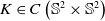 $ K\in C\left ({\mathbb{S}^2}\times {\mathbb{S}^2}\right )$
to be non-negative and satisfying
$ K\in C\left ({\mathbb{S}^2}\times {\mathbb{S}^2}\right )$
to be non-negative and satisfying $ \int _{\mathbb{S}^2} K(n,n')dn=1$
. We also assume in the whole article that the kernel
$ \int _{\mathbb{S}^2} K(n,n')dn=1$
. We also assume in the whole article that the kernel $ K$
is invariant under rotations, that is,
$ K$
is invariant under rotations, that is,
 \begin{equation*} K(n,n')=K({\mathcal{R}} n, {\mathcal{R}} n')\;\;\;\text{for all }n,n'\in {\mathbb{S}^2} \text{ and for any }{\mathcal{R}}\in SO(3). \end{equation*}
Moreover, for any $ n,\omega \in {\mathbb{S}^2}$
, we define by
$ n,\omega \in {\mathbb{S}^2}$
, we define by ${\mathcal{R}}_{n,\omega }\in SO(3)$
the rotation of
${\mathcal{R}}_{n,\omega }\in SO(3)$
the rotation of $ \pi$
around the bisectrix of the angle between
$ \pi$
around the bisectrix of the angle between $ n$
and
$ n$
and $ \omega$
lying in the plane containing both vectors. This rotation satisfies
$ \omega$
lying in the plane containing both vectors. This rotation satisfies $ {\mathcal{R}}_{n,\omega }(n)=\omega$
and
$ {\mathcal{R}}_{n,\omega }(n)=\omega$
and $ {\mathcal{R}}_{n,\omega }(\omega )=n$
. As shown in [Reference Demattè, Jang and Velázquez14], this implies that the scattering kernel
$ {\mathcal{R}}_{n,\omega }(\omega )=n$
. As shown in [Reference Demattè, Jang and Velázquez14], this implies that the scattering kernel $ K$
is symmetric. Notice that this is not true in two dimensions unless we assume
$ K$
is symmetric. Notice that this is not true in two dimensions unless we assume $ K$
to be invariant also under reflections.
$ K$
to be invariant also under reflections.
We define the scattering operator as the bounded linear operator given by
 \begin{equation} \begin{aligned} H\;:\;L^\infty \left ({\mathbb{S}^2}\right )& \to L^\infty \left ({\mathbb{S}^2}\right )\\[5pt] \varphi &\mapsto H[\varphi ]=\displaystyle\int _{\mathbb{S}^2} K(\cdot ,n')\varphi (n')\ dn'. \end{aligned} \end{equation}
With this notation, we can formulate the following proposition, which contains the most important properties of the scattering operator.
Proposition 2.1.
Let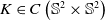 $ K\in C\left ({\mathbb{S}^2}\times {\mathbb{S}^2}\right )$
, invariant under rotations, non-negative and satisfying
$ K\in C\left ({\mathbb{S}^2}\times {\mathbb{S}^2}\right )$
, invariant under rotations, non-negative and satisfying
 \begin{equation*} \displaystyle\int _{\mathbb{S}^2} K(n,n')dn=1 .\end{equation*}
Assume $ \varphi \in L^\infty \left ({\mathbb{S}^2}\right )$
satisfies
$ \varphi \in L^\infty \left ({\mathbb{S}^2}\right )$
satisfies $ H[\varphi ]=\varphi$
. Then
$ H[\varphi ]=\varphi$
. Then
-
(i) $ \varphi$
is continuous,
$ \varphi$
is continuous,
-
(ii)
$ \varphi$
is constant,
-
(iii)
$ \text{Ran}(Id-H)=\left \{\varphi \in L^\infty ({\mathbb{S}^2}): \int _{\mathbb{S}^2} \varphi =0\right \}$
.



The proof of Proposition2.1 can be found in Appendix A. A direct consequence of Proposition2.1 is the following proposition for a continuous scattering kernel $ K\in C\left ({\mathbb{S}^2}\times {\mathbb{S}^2}\times \Omega \times {\mathbb{R}}_+\right )$
invariant under rotations for each pair
$ K\in C\left ({\mathbb{S}^2}\times {\mathbb{S}^2}\times \Omega \times {\mathbb{R}}_+\right )$
invariant under rotations for each pair $ (x,\nu )$
.
$ (x,\nu )$
.
Proposition 2.2.
Let $ K\in C\left ({\mathbb{S}^2}\times {\mathbb{S}^2}\times \Omega \times {\mathbb{R}}_+\right )$
. For any
$ K\in C\left ({\mathbb{S}^2}\times {\mathbb{S}^2}\times \Omega \times {\mathbb{R}}_+\right )$
. For any $ x,\nu \in \Omega \times {\mathbb{R}}_+$
, we define
$ x,\nu \in \Omega \times {\mathbb{R}}_+$
, we define $ K_{x,\nu }(n,n')=K(n,n',x,\nu )$
. Assume that for any
$ K_{x,\nu }(n,n')=K(n,n',x,\nu )$
. Assume that for any $ x,\nu \in \Omega \times {\mathbb{R}}_+$
, the kernel
$ x,\nu \in \Omega \times {\mathbb{R}}_+$
, the kernel $ K_{x,\nu }$
is invariant under rotations, is non-negative and satisfies
$ K_{x,\nu }$
is invariant under rotations, is non-negative and satisfies $ \int _{\mathbb{S}^2} K_{x,\nu }(n,n')dn=1 .$
Then the following holds.
$ \int _{\mathbb{S}^2} K_{x,\nu }(n,n')dn=1 .$
Then the following holds.
-
(i) For any
$ x,\nu \in \Omega \times {\mathbb{R}}_+$
and
$ n,\omega \in {\mathbb{S}^2}$
, there exist finitely many
$ n_1,\cdots ,n_N\in {\mathbb{S}^2}$
such that (
A.1
) holds for
$ K_{x,\nu }$
; -
(ii) if
$ \varphi \in L^\infty \left ({\mathbb{S}^2}\times \Omega \times {\mathbb{R}}_+\right )$
satisfies
$ H[\varphi ]=\varphi$
, then
$ \varphi$
is continuous, and it is constant for every
$ x,\nu \in \Omega \times {\mathbb{R}}_+$
, -
(iii)
$ \text{Ran}(Id-H)=\left \{\varphi (\cdot ,x,\nu )\in L^\infty ({\mathbb{S}^2}): \int _{\mathbb{S}^2} \varphi (n,x,\nu )\;dn=0\right \}$
for every
$ x,\nu \in \Omega \times {\mathbb{R}}_+$
.









Proof. Apply Proposition2.1 to the continuous kernel K x,ν .
Remark.
In the following sections, we will consider the diffusion approximation for scattering kernels $ K$
independent of
$ K$
independent of $ x\in \Omega$
and
$ x\in \Omega$
and $ \nu \geq 0$
. However, under the assumptions of Proposition
2.2
, the same results would apply for more general kernels depending continuously on
$ \nu \geq 0$
. However, under the assumptions of Proposition
2.2
, the same results would apply for more general kernels depending continuously on $ x$
and
$ x$
and $ \nu$
.
$ \nu$
.
Remark.
The assumption of $ K$
being invariant under rotations is crucial for the validity of Proposition
2.1
and Proposition
2.2
. Consider, for example, the following continuous function
$ K$
being invariant under rotations is crucial for the validity of Proposition
2.1
and Proposition
2.2
. Consider, for example, the following continuous function
 \begin{equation*}k(n)=\frac {2}{3\pi }\left ({ \chi }_{\left\{|n\cdot e_3|\leq \frac {1}{4}\right\}}(n)+(2-4|n\cdot e_3|){\chi }_{\left\{\frac {1}{4}\lt |n\cdot e_3|\lt \frac {1}{2}\right\}}(n)\right ). \end{equation*}
Then the kernel $K(n,n')=k(n){ \chi }_{{\mathbb{S}^2}}(n')$
is continuous in both variables, is non-negative and satisfies
$K(n,n')=k(n){ \chi }_{{\mathbb{S}^2}}(n')$
is continuous in both variables, is non-negative and satisfies
 \begin{equation*} \displaystyle\int _{\mathbb{S}^2} K(n,n')\, dn=\displaystyle\int _{\mathbb{S}^2} k(n)\, dn=1.\end{equation*}
However, $ K$
is not invariant under rotations. This kernel describes the scattering properties of a non-isotropic medium. It is easy to see that in this case
$ K$
is not invariant under rotations. This kernel describes the scattering properties of a non-isotropic medium. It is easy to see that in this case $ H[c](n)=ck(n)$
, for
$ H[c](n)=ck(n)$
, for $ c\in {\mathbb{R}}$
. Hence, the constant functions are not a solution to
$ c\in {\mathbb{R}}$
. Hence, the constant functions are not a solution to $ H[\varphi ]=\varphi$
. Actually, all solutions of
$ H[\varphi ]=\varphi$
. Actually, all solutions of $ H[\varphi ]=\varphi$
satisfy
$ H[\varphi ]=\varphi$
satisfy $ \varphi (n)=k(n)\int _{\mathbb{S}^2} \varphi (n')\;dn'$
and have hence the form
$ \varphi (n)=k(n)\int _{\mathbb{S}^2} \varphi (n')\;dn'$
and have hence the form $ \varphi =\lambda k$
, where
$ \varphi =\lambda k$
, where $ \lambda \in {\mathbb{R}}$
is an arbitrary constant. Therefore, the subspace of eigenvectors of
$ \lambda \in {\mathbb{R}}$
is an arbitrary constant. Therefore, the subspace of eigenvectors of $ H$
with eigenvalue
$ H$
with eigenvalue $ 1$
is one-dimensional.
$ 1$
is one-dimensional.
Remark.
As we noticed above, in two dimensions, the invariance under rotations of $ K$
does not imply directly its symmetry under reflections. However, it is still possible to show that the only eigenfunctions of
$ K$
does not imply directly its symmetry under reflections. However, it is still possible to show that the only eigenfunctions of $ H$
with eigenvalue 1 are the constants. To check this, we recall the well-known fact that the one-dimensional sphere
$ H$
with eigenvalue 1 are the constants. To check this, we recall the well-known fact that the one-dimensional sphere $ \mathbb{S}^1$
can be parameterized by
$ \mathbb{S}^1$
can be parameterized by $ \theta \in [0,2\pi )$
. Moreover, we can assume without loss of generality that any scattering kernel
$ \theta \in [0,2\pi )$
. Moreover, we can assume without loss of generality that any scattering kernel $ K$
invariant under rotations has the form
$ K$
invariant under rotations has the form $ K(n,n')=K(\theta (n)-\theta (n'))$
. Let
$ K(n,n')=K(\theta (n)-\theta (n'))$
. Let $ f\in L^\infty (\mathbb{S}^1)$
be an eigenfunction with eigenvalue 1 for
$ f\in L^\infty (\mathbb{S}^1)$
be an eigenfunction with eigenvalue 1 for $ H$
. We then see
$ H$
. We then see
 \begin{equation*} \displaystyle\int _0^{2\pi } K(\theta -\varphi )f(\varphi )\;d\varphi =f(\theta ). \end{equation*}
This equation can be solved using the Fourier series. We hence obtain the following identity for the Fourier coefficients
 \begin{equation} \hat {f}(n)\left (1-2\pi \hat {K}(n)\right )=0. \end{equation}
For $ n=0$
we have
$ n=0$
we have $ \hat {K}(0)=\frac {1}{2\pi }\int _0^{2\pi }K(\theta ) \;d\theta =\frac {1}{2\pi }$
. On the other hand, we obtain for
$ \hat {K}(0)=\frac {1}{2\pi }\int _0^{2\pi }K(\theta ) \;d\theta =\frac {1}{2\pi }$
. On the other hand, we obtain for $ n\ne 0$
 \begin{equation*} \left |\hat {K}(n)\right |\lt \frac {1}{2\pi }\displaystyle\int _0^{2\pi }K(\theta )\;d\theta =\frac {1}{2\pi }. \end{equation*}
Therefore, the identity (
2.2
) is satisfied if and only if $ \hat {f}(n)=0$
for all
$ \hat {f}(n)=0$
for all $ n\ne 0$
. This implies that
$ n\ne 0$
. This implies that $ f$
is constant.
$ f$
is constant.
2.2. Relation between the temperature and the radiation intensity
We derive here an identity that relates temperature and radiation intensity and that will be repeatedly used in the stationary problem, for instance, in the stationary boundary layer equations.
Using the identity $ \textrm {div}\left (\int _0^\infty d\nu \int _{\mathbb{S}^2} dn\;nI_\nu (x,n)\right )=\int _0^\infty d\nu \int _{\mathbb{S}^2} dn\;n\cdot \nabla _xI_\nu (x,n)$
and plugging the first equation of (1.5) into the second one, we see that we have
$ \textrm {div}\left (\int _0^\infty d\nu \int _{\mathbb{S}^2} dn\;nI_\nu (x,n)\right )=\int _0^\infty d\nu \int _{\mathbb{S}^2} dn\;n\cdot \nabla _xI_\nu (x,n)$
and plugging the first equation of (1.5) into the second one, we see that we have
 \begin{equation} \displaystyle\int _0^\infty d\nu \displaystyle\int _{\mathbb{S}^2} dn\; \alpha _\nu ^a(x)\left (B_\nu (T(x))-I_\nu (x,n)\right ) =0, \end{equation}
where we also used the fact that the integral over the sphere $ {\mathbb{S}^2}$
of the scattering term is
$ {\mathbb{S}^2}$
of the scattering term is $ 0$
due to the symmetry of the kernel
$ 0$
due to the symmetry of the kernel $ K$
. With this identity, we can recover the value of the temperature given the radiation intensity. Let us define by
$ K$
. With this identity, we can recover the value of the temperature given the radiation intensity. Let us define by $ F\;:\;{\mathbb{R}}_+\times \Omega \to {\mathbb{R}}_+$
the following function
$ F\;:\;{\mathbb{R}}_+\times \Omega \to {\mathbb{R}}_+$
the following function
 \begin{equation} F(T,x)=\displaystyle\int _0^\infty \alpha _\nu ^a(x)B_\nu (T)\;d\nu . \end{equation}
Since $ B_\nu$
is monotone in
$ B_\nu$
is monotone in $ T$
, the function
$ T$
, the function $ F(\cdot , x)$
is invertible. Hence, (2.3) implies that
$ F(\cdot , x)$
is invertible. Hence, (2.3) implies that
 \begin{equation} T(x)=F^{-1}\left (\left (\displaystyle\int _0^\infty d\nu {\displaystyle\int\!\!\!\!\!\!\diagup}_{\mathbb{S}^2} dn\; \alpha _\nu ^a(x)I_\nu (x,n)\right ),x\right ), \end{equation}
where $ F^{-1}$
is the inverse with respect to the first variable; that is,
$ F^{-1}$
is the inverse with respect to the first variable; that is, $ F(T,x)=\xi$
implies
$ F(T,x)=\xi$
implies $ T=F^{-1}(\xi ,x)$
. Equations (2.3) and (2.5) will appear often in the following sections, in particular in the study of the boundary layers.
$ T=F^{-1}(\xi ,x)$
. Equations (2.3) and (2.5) will appear often in the following sections, in particular in the study of the boundary layers.
3. The stationary diffusion approximation: different scales
We first study the stationary diffusion regime for different scalings. We consider (1.12) for $ \alpha _\nu ^a$
and
$ \alpha _\nu ^a$
and $ \alpha _\nu ^s$
strictly positive and bounded. Moreover, in the diffusion regime, we have
$ \alpha _\nu ^s$
strictly positive and bounded. Moreover, in the diffusion regime, we have $ \ell _M\ll 1$
. Hence, in (1.12), we assume
$ \ell _M\ll 1$
. Hence, in (1.12), we assume $ \ell _M=\min \{\ell _A,\ell _S\}=\varepsilon$
. Moreover, we impose
$ \ell _M=\min \{\ell _A,\ell _S\}=\varepsilon$
. Moreover, we impose $ \ell _A=\varepsilon ^{-\beta }$
and
$ \ell _A=\varepsilon ^{-\beta }$
and $ \ell _S=\varepsilon ^{-\gamma }$
, for suitable choices of
$ \ell _S=\varepsilon ^{-\gamma }$
, for suitable choices of $ \gamma ,\beta \geq -1$
with
$ \gamma ,\beta \geq -1$
with $ \min \{\gamma , \beta \}=-1$
. Notice that at least one of
$ \min \{\gamma , \beta \}=-1$
. Notice that at least one of $ \beta$
and
$ \beta$
and $ \gamma$
is negative. This choice of
$ \gamma$
is negative. This choice of $ \ell _A$
and
$ \ell _A$
and $ \ell _S$
as an inverse power law of
$ \ell _S$
as an inverse power law of $ \varepsilon \gt 0$
for
$ \varepsilon \gt 0$
for $ \beta , \gamma \geq -1$
will be convenient in order to make the computations simpler in the following subsections. Under these assumptions, we rewrite equation (1.12) as
$ \beta , \gamma \geq -1$
will be convenient in order to make the computations simpler in the following subsections. Under these assumptions, we rewrite equation (1.12) as
 \begin{equation} \begin{cases} n\cdot \nabla _x I_\nu (x,n)=\varepsilon ^\beta \alpha _\nu ^a(x)\left (B_\nu (T(x))-I_\nu (x,n)\right )\\[5pt] {\phantom {nel mezzo del cammin }}+\varepsilon ^\gamma \alpha _\nu ^s(x)\left (\displaystyle\int _{\mathbb{S}^2} K(n,n')I_\nu (x,n')\;dn'-I_\nu (x,n)\right )&x\in \Omega ,n\in {\mathbb{S}^2}\\[5pt] \textrm {div}\left (\displaystyle\int _0^\infty d\nu \displaystyle\int _{\mathbb{S}^2} dn \;nI_\nu (n,x)\right )=0&x\in \Omega ,n\in {\mathbb{S}^2}\\[5pt] I_\nu (n,x)=g_\nu (n)&x\in {\partial \Omega },n\cdot n_x\lt 0. \end{cases} \end{equation}
Moreover, we assume the scattering kernel $ K\in C({\mathbb{S}^2}\times {\mathbb{S}^2})$
to be invariant under rotations, non-negative and with
$ K\in C({\mathbb{S}^2}\times {\mathbb{S}^2})$
to be invariant under rotations, non-negative and with $ \int _{\mathbb{S}^2} K(n,n')dn=1$
. We consider also
$ \int _{\mathbb{S}^2} K(n,n')dn=1$
. We consider also $ \Omega \subset {\mathbb{R}}^3$
to be a bounded convex domain with
$ \Omega \subset {\mathbb{R}}^3$
to be a bounded convex domain with $ C^1$
-boundary. For
$ C^1$
-boundary. For $ x\in {\partial \Omega }$
, we denote by
$ x\in {\partial \Omega }$
, we denote by $ n_x\in {\mathbb{S}^2}$
the outer normal to the boundary at
$ n_x\in {\mathbb{S}^2}$
the outer normal to the boundary at $ x$
.
$ x$
.
Before describing in detail the limit diffusion problems for the different choices of scaling parameters, we shortly explain how we will use the method of matched asymptotic expansions to derive the limit problems for each case. In order to find the limit problem valid in the bulk, the so-called outer problem, we expand the radiation intensity as
 \begin{equation} I_\nu (x,n)=\phi _0(x,n,\nu )+\sum _{k\geq 0} \varepsilon ^{\delta +k}\psi _{k+1}(x,n,\nu )+\sum _{l\gt 0} \varepsilon ^l \phi _l(x,n,\nu ) \end{equation}
for a suitable $ \delta \gt 0$
depending on the choice of the scaling parameters. To be more precise,
$ \delta \gt 0$
depending on the choice of the scaling parameters. To be more precise,
 \begin{equation} \delta =\begin{cases}\gamma +1 & \text{ if }\beta =-1\text{ (i.e. }\ell _A=\ell _M),\\[5pt] \beta -\lfloor \beta \rfloor & \text{ if }\gamma =-1\text{ (i.e. }\ell _S=\ell _M). \end{cases} \end{equation}
We remark that if $-1\lt \beta \lt 0$
, by our definition,
$-1\lt \beta \lt 0$
, by our definition, $ \delta =\beta +1\gt 0$
. The choice of
$ \delta =\beta +1\gt 0$
. The choice of $ \delta$
in (3.2) is due to the following observations. If
$ \delta$
in (3.2) is due to the following observations. If $ \ell _A=\ell _M$
, the leading term of the radiative transfer equation is the emission-absorption term, so that
$ \ell _A=\ell _M$
, the leading term of the radiative transfer equation is the emission-absorption term, so that
 \begin{equation*}\alpha _\nu ^a(x)(I_\nu (x,n)-B_\nu (T(x)))=\varepsilon n\cdot \nabla _xI_\nu (x,n)-\alpha _\nu ^s(x)\varepsilon ^{\gamma +1}(H-Id)[I_\nu (x,\cdot )](n),\end{equation*}
where we used the notation of (2.1). Therefore, it is natural to look for a solution of this equation in form of a series of powers of $ \varepsilon$
with exponents
$ \varepsilon$
with exponents $ 1$
and
$ 1$
and $ \gamma +1$
. On the other hand, if
$ \gamma +1$
. On the other hand, if $ \ell _S=\ell _M$
, the leading term is the scattering term yielding
$ \ell _S=\ell _M$
, the leading term is the scattering term yielding
 \begin{equation*}\alpha _\nu ^s(x)(H-Id)[I_\nu (x,\cdot )](n)=\varepsilon n\cdot \nabla _xI_\nu (x,n)-\varepsilon ^{\beta +1}\alpha _\nu ^a(x)(I_\nu (x,n)-B_\nu (T(x))).\end{equation*}
As we have seen in Proposition2.1, the solvability of this equation requires to impose a compatibility condition on the right-hand side. More precisely, $ (Id-H)$
is invertible in the space of functions with
$ (Id-H)$
is invertible in the space of functions with $ \int _{{\mathbb{S}^2}} f(n)dn=0$
. This compatibility condition is provided by the transport term
$ \int _{{\mathbb{S}^2}} f(n)dn=0$
. This compatibility condition is provided by the transport term $ \varepsilon n\cdot \nabla _x I_\nu (x,n)$
. In particular, the relevant feature is that the problem
$ \varepsilon n\cdot \nabla _x I_\nu (x,n)$
. In particular, the relevant feature is that the problem
 \begin{equation} \alpha _\nu ^s(x)(H-Id)[I_\nu (x,\cdot )](n)-\varepsilon n\cdot \nabla _xI_\nu (x,n)=f(x,n,\nu ) \end{equation}
is not solvable if $ \varepsilon =0$
, unless
$ \varepsilon =0$
, unless $ \int _{\mathbb{S}^2} f(x,n,\nu ) dn=0$
. On the contrary, in the case of
$ \int _{\mathbb{S}^2} f(x,n,\nu ) dn=0$
. On the contrary, in the case of $ \varepsilon \gt 0$
and small, it turns out that problem (3.4) can be solved for general
$ \varepsilon \gt 0$
and small, it turns out that problem (3.4) can be solved for general $ f$
. However, the solution becomes of the order
$ f$
. However, the solution becomes of the order $ \varepsilon ^{-2} \Arrowvert f\Arrowvert _\infty$
. This explains why we have to add terms much larger than
$ \varepsilon ^{-2} \Arrowvert f\Arrowvert _\infty$
. This explains why we have to add terms much larger than $ \varepsilon ^{\beta +1}$
in the expansion (3.2) for
$ \varepsilon ^{\beta +1}$
in the expansion (3.2) for $ \beta \gt 0$
. We remark that the expansion (3.2) is also used in the time-dependent case. There, the value of
$ \beta \gt 0$
. We remark that the expansion (3.2) is also used in the time-dependent case. There, the value of $ \delta$
when
$ \delta$
when $ \ell _S=\ell _M$
is justified by the behaviour of the radiation intensity for smaller time scales and by the need to impose this orthogonality condition.
$ \ell _S=\ell _M$
is justified by the behaviour of the radiation intensity for smaller time scales and by the need to impose this orthogonality condition.
Having expansion (3.2), we proceed by plugging it into the boundary value problem (1.12), and we compare all terms of the same order of magnitude. In this way, we will obtain different diffusive equations solved by $ \phi _0$
in the interior of
$ \phi _0$
in the interior of $ \Omega$
that will yield the leading order of the radiation intensity
$ \Omega$
that will yield the leading order of the radiation intensity $ I_\nu$
.
$ I_\nu$
.
However, to solve the resulting equation for $ \phi _0$
, we need some boundary condition whose derivation requires to analyse boundary layer equations for (3.1). The resulting boundary layer problems are related to the description of the radiation intensity in the regions close to the boundary. The thickness of these layers is given by the Milne length and the thermalization length. Therefore, we will rescale the space variable according to
$ \phi _0$
, we need some boundary condition whose derivation requires to analyse boundary layer equations for (3.1). The resulting boundary layer problems are related to the description of the radiation intensity in the regions close to the boundary. The thickness of these layers is given by the Milne length and the thermalization length. Therefore, we will rescale the space variable according to $ \ell _M$
and to
$ \ell _M$
and to $ \ell _T$
, and we will analyse the resulting one-dimensional problems.
$ \ell _T$
, and we will analyse the resulting one-dimensional problems.
The matching between the outer and the inner solutions will provide the boundary condition for the equation satisfied in the bulk.
3.1. Case 1.1:
$ \ell _M=\ell _T\ll \ell _S$
and
$ L=1$
. Equilibrium approximation


Since we set $ \ell _M=\varepsilon \ll 1$
, the case
$ \ell _M=\varepsilon \ll 1$
, the case $ \ell _M=\ell _T\ll \ell _S$
arises when
$ \ell _M=\ell _T\ll \ell _S$
arises when $ \ell _A=\varepsilon$
(i.e.
$ \ell _A=\varepsilon$
(i.e. $ \beta =-1$
) and
$ \beta =-1$
) and $ \ell _S=\varepsilon ^{-\gamma }$
for
$ \ell _S=\varepsilon ^{-\gamma }$
for $ \gamma \gt -1$
. Notice that in this case
$ \gamma \gt -1$
. Notice that in this case $ \ell _S$
could be small, namely,
$ \ell _S$
could be small, namely, $ \ell _S\ll L=1$
, but also large, for example, if
$ \ell _S\ll L=1$
, but also large, for example, if $ \gamma \gt 0$
.
$ \gamma \gt 0$
.
In order to find the outer problem, we choose $ \delta = \gamma +1$
, and we substitute (3.2) into the first equation in (3.1), and we identify all terms with the same power of
$ \delta = \gamma +1$
, and we substitute (3.2) into the first equation in (3.1), and we identify all terms with the same power of $ \varepsilon$
, that is,
$ \varepsilon$
, that is, $ \varepsilon ^{-1}$
,
$ \varepsilon ^{-1}$
, $ \varepsilon ^{\gamma }$
(if
$ \varepsilon ^{\gamma }$
(if $ -1\lt \gamma \lt 0$
) and
$ -1\lt \gamma \lt 0$
) and $ \varepsilon ^0$
. If
$ \varepsilon ^0$
. If $ -1\lt \gamma \lt 0$
, the terms of order
$ -1\lt \gamma \lt 0$
, the terms of order $ \varepsilon ^{-1}$
give
$ \varepsilon ^{-1}$
give
 \begin{equation*} 0=\alpha _\nu ^a(x)(B_\nu (T(x))-\phi _0(x,n,\nu )). \end{equation*}
Hence, the leading order satisfies $ \phi _0(x,n,\nu )=B_\nu (T(x))$
, where
$ \phi _0(x,n,\nu )=B_\nu (T(x))$
, where $ B_\nu$
is the Planck distribution, which is independent of
$ B_\nu$
is the Planck distribution, which is independent of $ n\in {\mathbb{S}^2}$
. This corresponds to the diffusion equilibrium approximation, since in the interior, the radiation intensity is at the leading order the equilibrium Planck distribution.
$ n\in {\mathbb{S}^2}$
. This corresponds to the diffusion equilibrium approximation, since in the interior, the radiation intensity is at the leading order the equilibrium Planck distribution.
The terms of order $ \varepsilon ^\gamma$
imply
$ \varepsilon ^\gamma$
imply $ \psi _1=0$
. Indeed, since
$ \psi _1=0$
. Indeed, since $ \phi _0(x,n,\nu )=B_\nu (T(x))$
is independent of
$ \phi _0(x,n,\nu )=B_\nu (T(x))$
is independent of $ n\in {\mathbb{S}^2}$
, we have
$ n\in {\mathbb{S}^2}$
, we have $ \int _{\mathbb{S}^2} K(n,n')\phi _0(x,\nu )dn'-\phi _0(x,\nu )=0$
, so that
$ \int _{\mathbb{S}^2} K(n,n')\phi _0(x,\nu )dn'-\phi _0(x,\nu )=0$
, so that
 \begin{equation*}\alpha _\nu ^a\psi _1(x,n,\nu )=\displaystyle\int _{\mathbb{S}^2} K(n,n')\phi _0(x,\nu )dn'-\phi _0(x,\nu )=0.\end{equation*}
Finally, we compare all terms of order $ \varepsilon ^0$
. In this case, we have
$ \varepsilon ^0$
. In this case, we have
 \begin{equation*} n\cdot \nabla _x B_\nu (T(x))=-\alpha _\nu ^a(x)\phi _{1}(x,n,\nu ), \end{equation*}
where in the case $ \gamma =0$
, we used again that
$ \gamma =0$
, we used again that $ \left (H-Id\right )B_\nu (T)=0$
.
$ \left (H-Id\right )B_\nu (T)=0$
.
Therefore, we obtain the following expansion for $ I_\nu$
 \begin{equation} I_\nu (x,n)=B_\nu (T(x))-\varepsilon \frac {1}{\alpha ^{a}_\nu (x)}n\cdot \nabla _x B_\nu (T(x))+\cdots , \end{equation}
where $ T(x)$
is a function, which is at this stage still unknown.
$ T(x)$
is a function, which is at this stage still unknown.
We now plug (3.5) into the second equation of (3.1). The term of order $ \varepsilon ^0$
cancels out because
$ \varepsilon ^0$
cancels out because $ B_\nu (T)$
is isotropic, hence
$ B_\nu (T)$
is isotropic, hence
 \begin{equation*} \textrm {div}\left (\displaystyle\int _0^\infty d\nu \displaystyle\int _{{\mathbb{S}^2}} dn\;n B_\nu (T(x))\right )=0.\end{equation*}
We find that the leading term is the one of order $ \varepsilon ^1$
, and we obtain
$ \varepsilon ^1$
, and we obtain
 \begin{equation*} \textrm {div} \left (\displaystyle\int _0^\infty d\nu \frac {1}{\alpha _\nu (x)}\left (\displaystyle\int _{\mathbb{S}^2} dn\; n\otimes n\right )\nabla _x B_\nu (T(x))\right )=0. \end{equation*}
Finally, using that $ \int _{\mathbb{S}^2} n\otimes n\;dn=\frac {4\pi }{3}Id$
, we conclude that the limit problem solved at the interior by
$ \int _{\mathbb{S}^2} n\otimes n\;dn=\frac {4\pi }{3}Id$
, we conclude that the limit problem solved at the interior by $ T$
is
$ T$
is
 \begin{equation} \textrm {div}\left (\displaystyle\int _0^\infty \frac {\nabla _x B_\nu (T(x))}{\alpha _\nu (x)}d\nu \right )=0. \end{equation}
In order to obtain the behaviour of $ I_\nu$
close to the boundary
$ I_\nu$
close to the boundary $ {\partial \Omega }$
, we now derive a boundary value problem that can be written in a single variable. This boundary layer equation is known in the literature as the Milne problem. The matching of the solution of the Milne problem with the outer solution will provide the boundary value for the equation (3.6) solved by the temperature
$ {\partial \Omega }$
, we now derive a boundary value problem that can be written in a single variable. This boundary layer equation is known in the literature as the Milne problem. The matching of the solution of the Milne problem with the outer solution will provide the boundary value for the equation (3.6) solved by the temperature $ T$
.
$ T$
.
We take $ p\in {\partial \Omega }$
. Assuming that near the boundary the radiation intensity and the temperature only depend on the distance to the boundary, we can further assume that they depend only on the distance to the boundary in direction
$ p\in {\partial \Omega }$
. Assuming that near the boundary the radiation intensity and the temperature only depend on the distance to the boundary, we can further assume that they depend only on the distance to the boundary in direction $ n_p$
. This is possible due to the smallness of the thickness of the boundary layer and the continuity of
$ n_p$
. This is possible due to the smallness of the thickness of the boundary layer and the continuity of $ \alpha$
. We hence define for
$ \alpha$
. We hence define for $ x \in \Omega$
in a neighbourhood of
$ x \in \Omega$
in a neighbourhood of $ p$
the new scalar rescaled variable
$ p$
the new scalar rescaled variable
 \begin{equation} y=-\frac {x-p}{\varepsilon }\cdot n_p. \end{equation}
We recall that $ -(x-p)\cdot n_p$
is non-negative, since
$ -(x-p)\cdot n_p$
is non-negative, since $ x-p$
points in the interior of the domain, and it is exactly the length of the cathetus with endpoint
$ x-p$
points in the interior of the domain, and it is exactly the length of the cathetus with endpoint $ p$
of the triangle having as hypotenuse
$ p$
of the triangle having as hypotenuse $ x-p$
(cf. Figure 1).
$ x-p$
(cf. Figure 1).
Representation of the change of variables.

Defining $ {\mathcal{R}}_p(x)={\text{Rot}}_p (x-p)$
as a rigid motion mapping
$ {\mathcal{R}}_p(x)={\text{Rot}}_p (x-p)$
as a rigid motion mapping $ p$
to zero with
$ p$
to zero with $ {\text{Rot}}_p(n_p)=-e_1$
, we see that we can also write
$ {\text{Rot}}_p(n_p)=-e_1$
, we see that we can also write $ y$
as the first component of
$ y$
as the first component of $ y_1={\mathcal{R}}_p\left (\frac {x}{\varepsilon }\right )_1$
. Hence, as
$ y_1={\mathcal{R}}_p\left (\frac {x}{\varepsilon }\right )_1$
. Hence, as $ \varepsilon \to 0$
, we obtain that both the absorption and the scattering coefficients satisfy
$ \varepsilon \to 0$
, we obtain that both the absorption and the scattering coefficients satisfy $ \alpha ^j_\nu (x)=\alpha ^j_\nu \left (\varepsilon {\text{Rot}}_p(x)+p\right )\to \alpha ^j_\nu (p)$
,
$ \alpha ^j_\nu (x)=\alpha ^j_\nu \left (\varepsilon {\text{Rot}}_p(x)+p\right )\to \alpha ^j_\nu (p)$
, $ j\in \{a,s\}$
.
$ j\in \{a,s\}$
.
We can now write the one-dimensional problem obtained by this new scaling and by the limit $ \varepsilon \to 0$
. Since
$ \varepsilon \to 0$
. Since $ \varepsilon ^{\gamma +1}\to 0$
as
$ \varepsilon ^{\gamma +1}\to 0$
as $ \varepsilon \to 0$
, the scattering term is negligible, and we obtain for any
$ \varepsilon \to 0$
, the scattering term is negligible, and we obtain for any $ p\in {\partial \Omega }$
 \begin{equation} \begin{cases} -(n\cdot n_p)\partial _yI_\nu (y,n;\;p)=\alpha _\nu ^a(p)(B_\nu (T(y,p))-I_\nu (y,n;\;p))& y\gt 0\;,n\in {\mathbb{S}^2}\\[5pt] \textrm {div}\left (\displaystyle\int _0^\infty d\nu \displaystyle\int _{\mathbb{S}^2} dn\; (n\cdot n_p) I_\nu (y,n;\;p)\right )=0&y\gt 0,\;n\in {\mathbb{S}^2}\\[5pt] I_\nu (0,n;\;p)=g_\nu (n)& n\cdot n_p\lt 0. \end{cases} \end{equation}
The Milne equation (3.8) is the equation describing the boundary layer for the diffusion approximation. In the pure absorption case, the Milne problem was rigorously studied in [Reference Golse25]. The well-posedness of (3.8) is shown there for constant absorption coefficients and also for coefficients depending only on the frequency $ \nu$
, as well as for coefficients depending on both frequency and temperature of the form
$ \nu$
, as well as for coefficients depending on both frequency and temperature of the form $ \alpha ^a_\nu (p)=Q(\nu )\alpha (T(p)).$
Moreover, the asymptotic behaviour of
$ \alpha ^a_\nu (p)=Q(\nu )\alpha (T(p)).$
Moreover, the asymptotic behaviour of $ I_\nu$
at infinity has also been computed in this paper. It is indeed shown in [Reference Golse25] that as
$ I_\nu$
at infinity has also been computed in this paper. It is indeed shown in [Reference Golse25] that as $ y\to \infty$
, the solution of the Milne problem converges to the Planck distribution, that is,
$ y\to \infty$
, the solution of the Milne problem converges to the Planck distribution, that is,
 \begin{equation*} \lim \limits _{y\to \infty } I_\nu (y,n;\;p)=I^\infty _\nu (p)=B_\nu (T_\infty (p)), \end{equation*}
for some $ T_\infty (p)$
depending only on
$ T_\infty (p)$
depending only on $ g_\nu$
and
$ g_\nu$
and $ p$
. Notice that
$ p$
. Notice that $ I_\nu ^\infty (p)$
is independent of
$ I_\nu ^\infty (p)$
is independent of $ n\in {\mathbb{S}^2}$
.
$ n\in {\mathbb{S}^2}$
.
Moreover, since in this case the thermalization length and the Milne length are the same, this is the only boundary layer appearing. The radiation intensity $ I_\nu$
becomes simultaneously isotropic and at equilibrium
$ I_\nu$
becomes simultaneously isotropic and at equilibrium $ B_\nu (T)$
in the same length scale. This gives a matching condition for the temperature that has to be used as a boundary condition for the new limit problem. In particular, the temperature and the radiation intensity solving the Milne problem (3.8) are related by equation (2.3). In particular,
$ B_\nu (T)$
in the same length scale. This gives a matching condition for the temperature that has to be used as a boundary condition for the new limit problem. In particular, the temperature and the radiation intensity solving the Milne problem (3.8) are related by equation (2.3). In particular,
 \begin{equation} T_\infty (p)=\lim \limits _{y\to \infty }F^{-1}\left (\left (\displaystyle\int _0^\infty d\nu \alpha _\nu ^a(p) I_\nu ^\infty (p)\right ),p\right ), \end{equation}
where $ F$
is defined in (2.4) and
$ F$
is defined in (2.4) and $ g\mapsto I^\infty _\nu (p)$
is a functional that determines the limit intensity for each boundary point
$ g\mapsto I^\infty _\nu (p)$
is a functional that determines the limit intensity for each boundary point $ p\in {\partial \Omega }$
.
$ p\in {\partial \Omega }$
.
Summarizing, the limit problem for the stationary radiative transfer equation (1.12) in the case $ \ell _M=\ell _T\ll \ell _S$
is given by the following boundary value problem
$ \ell _M=\ell _T\ll \ell _S$
is given by the following boundary value problem
 \begin{equation*} \begin{cases} \textrm {div}\left (\displaystyle\int _0^\infty \dfrac {\nabla _x B_\nu (T(x))}{\alpha _\nu (x)}d\nu \right )=0& x\in \Omega \\[5pt] T(p)=T_\infty (p)& p\in {\partial \Omega }, \end{cases} \end{equation*}
where $ T_\infty (p)$
is given by (3.9).
$ T_\infty (p)$
is given by (3.9).
3.2. Case 1.2:
$ \ell _M=\ell _T=\ell _S\ll L$
. Equilibrium approximation

Due to the definitions $ \ell _M=\varepsilon \ll 1$
and
$ \ell _M=\varepsilon \ll 1$
and $ \ell _T=\sqrt {\ell _A \ell _M}$
, we have
$ \ell _T=\sqrt {\ell _A \ell _M}$
, we have $ \ell _M=\ell _S=\ell _T=\ell _A=\varepsilon$
in (1.12), that is,
$ \ell _M=\ell _S=\ell _T=\ell _A=\varepsilon$
in (1.12), that is, $ \beta =\gamma =-1$
in (3.1).
$ \beta =\gamma =-1$
in (3.1).
We consider the expansion (3.2) for $ \delta =0$
, or equivalently without the expansion
$ \delta =0$
, or equivalently without the expansion $ \sum _{k\geq 0}\varepsilon ^{\delta +k} \psi _{k+1}$
. We plug (3.2) into (3.1), and we compare all terms of the same power of
$ \sum _{k\geq 0}\varepsilon ^{\delta +k} \psi _{k+1}$
. We plug (3.2) into (3.1), and we compare all terms of the same power of $ \varepsilon$
, namely,
$ \varepsilon$
, namely, $ \varepsilon ^{-1}$
and
$ \varepsilon ^{-1}$
and $ \varepsilon ^0$
. The term of order
$ \varepsilon ^0$
. The term of order $ \varepsilon ^{-1}$
yields
$ \varepsilon ^{-1}$
yields
 \begin{equation} 0=\alpha _\nu ^a(x)(B_\nu (T(x))-\phi _0(x,n,\nu ))+\alpha _\nu ^s(x)\left (\displaystyle\int _{\mathbb{S}^2} K(n,n') \phi _0(x,n',\nu )dn'-\phi _0(x,n,\nu )\right ). \end{equation}
Notice that $ \phi _0(x,n,\nu )=B_\nu (T(x))$
is a solution to (3.10). This follows from Proposition2.1 and the isotropy of
$ \phi _0(x,n,\nu )=B_\nu (T(x))$
is a solution to (3.10). This follows from Proposition2.1 and the isotropy of $ B_\nu (T)$
. We show now that the solution to (3.10) is unique.
$ B_\nu (T)$
. We show now that the solution to (3.10) is unique.
To this end, for every $ x\in {\mathbb{R}}^3$
and
$ x\in {\mathbb{R}}^3$
and $ \nu \gt 0$
, we define
$ \nu \gt 0$
, we define $ 0\lt \theta _{\nu ,x}=\frac {\alpha _\nu ^s(x)}{\alpha _\nu ^a(x)+\alpha _\nu ^s(x)}\lt 1$
. Moreover, we also define the following operator, which maps for every fixed
$ 0\lt \theta _{\nu ,x}=\frac {\alpha _\nu ^s(x)}{\alpha _\nu ^a(x)+\alpha _\nu ^s(x)}\lt 1$
. Moreover, we also define the following operator, which maps for every fixed $ x,\nu$
non-negative continuous functions to non-negative continuous functions and which is given by
$ x,\nu$
non-negative continuous functions to non-negative continuous functions and which is given by
 \begin{equation} A_{\nu ,x}[\varphi ](n)=\theta _{\nu ,x}\displaystyle\int _{\mathbb{S}^2} K(n,n')\varphi (n')\;dn'. \end{equation}
Then equation (3.10) can be rewritten as
 \begin{equation} \phi _0(x,n,\nu )=A_{\nu ,x}[\phi _0](x,n,\nu )+\frac {\alpha _\nu ^a(x)}{\alpha _\nu ^a(x)+\alpha _\nu ^s(x)}B_\nu (T(x)). \end{equation}
Since the maps $ \phi _0\mapsto A_{\nu ,x}(\phi _0)$
is a linear contraction, the Banach fixed-point theorem implies that (3.12) has a unique solution for every
$ \phi _0\mapsto A_{\nu ,x}(\phi _0)$
is a linear contraction, the Banach fixed-point theorem implies that (3.12) has a unique solution for every $ T(x)\in {\mathbb{R}}_+$
. Hence,
$ T(x)\in {\mathbb{R}}_+$
. Hence, $ \phi _0=B_\nu (T)$
. Therefore, in this case, we also recover the equilibrium diffusion approximation.
$ \phi _0=B_\nu (T)$
. Therefore, in this case, we also recover the equilibrium diffusion approximation.
We turn now to the terms of order $\varepsilon ^0$
. In this case, we have
$\varepsilon ^0$
. In this case, we have
 \begin{equation*} n\cdot \nabla _x B_\nu (T(x))=-\alpha _\nu ^a(x)\phi _1(x,n,\nu )-\alpha _\nu ^s(x)\left (\displaystyle\int _{\mathbb{S}^2} K(n,n')\phi _1(x,n',\nu )\;dn'-\phi _1(x,n,\nu )\right ). \end{equation*}
Then, using the operator $ A_{\nu ,x}$
defined as in (3.11), we can rewrite this equation as
$ A_{\nu ,x}$
defined as in (3.11), we can rewrite this equation as
 \begin{equation} -\frac {1}{\alpha _\nu ^a(x)+\alpha _\nu ^s(x)}n\cdot \nabla _x B_\nu (T(x))=\left (Id-A_{\nu ,x}\right )\phi _1(x,n,\nu ). \end{equation}
The same argument as for the term of order $ \varepsilon ^{-1}$
holds also in this case, and the Banach fixed-point theorem ensures the existence of a unique solution to (3.13) given by
$ \varepsilon ^{-1}$
holds also in this case, and the Banach fixed-point theorem ensures the existence of a unique solution to (3.13) given by
 \begin{equation*} \phi _1(x,n,\nu )=-\frac {1}{\alpha _\nu ^a(x)+\alpha _\nu ^s(x)}\left (Id-A_{\nu ,x}\right )^{-1}(n)\cdot \nabla _x B_\nu (T(x)), \end{equation*}
where for any $ x,\nu$
, we used the notation
$ x,\nu$
, we used the notation
 \begin{equation*} \left (Id-A_{\nu ,x}\right )^{-1}(n)=\begin{pmatrix} \left (Id-A_{\nu ,x}\right )^{-1}(n_1)\\[5pt] \left (Id-A_{\nu ,x}\right )^{-1}(n_2)\\[5pt] \left (Id-A_{\nu ,x}\right )^{-1}(n_3) \end{pmatrix}, \end{equation*}
which is well-defined due to the action of the linear operator $ A_{\nu ,x}$
only on the variable
$ A_{\nu ,x}$
only on the variable $ n\in {\mathbb{S}^2}$
.
$ n\in {\mathbb{S}^2}$
.
Hence, we obtain the following expansion
 \begin{equation} I_\nu (x,n)=B_\nu (T(x))-\varepsilon \frac {1}{\alpha _\nu ^a(x)+\alpha _\nu ^s(x)}\left (Id-A_{\nu ,x}\right )^{-1}(n)\cdot \nabla _x B_\nu (T(x))+\varepsilon ^2\phi _2+\cdots \end{equation}
Plugging (3.14) into the second equation of (1.12) and using that the Planck distribution is isotropic, we obtain the following limit problem solved in the domain $ \Omega$
that yields the temperature
$ \Omega$
that yields the temperature $ T(x)$
to the leading order
$ T(x)$
to the leading order
 \begin{equation} \begin{aligned} 0&=\textrm {div} \left (\displaystyle\int _0^\infty d\nu \displaystyle\int _{\mathbb{S}^2} dn\; n\frac {1}{\alpha _\nu ^a(x)+\alpha _\nu ^s(x)}\left (Id-A_{\nu ,x}\right )^{-1}(n)\cdot \nabla _x B_\nu (T(x))\right )\\[5pt] &=\textrm {div} \left (\displaystyle\int _0^\infty d\nu \frac {1}{\alpha _\nu ^a(x)+\alpha _\nu ^s(x)}\left (\displaystyle\int _{\mathbb{S}^2} dn\; n\otimes \left (Id-A_{\nu ,x}\right )^{-1}(n)\right )\nabla _x B_\nu (T(x))\right ). \end{aligned} \end{equation}
The behaviour of $ I_\nu$
close to the boundary
$ I_\nu$
close to the boundary $ {\partial \Omega }$
is given again by a boundary layer equation, which can be written in one variable. The derivation of the Milne problem for this case follows exactly the same steps as Subsection 3.1 under the scaling (3.7). In this case, both emission and scattering terms appear, since they are of the same order. Hence, for every
$ {\partial \Omega }$
is given again by a boundary layer equation, which can be written in one variable. The derivation of the Milne problem for this case follows exactly the same steps as Subsection 3.1 under the scaling (3.7). In this case, both emission and scattering terms appear, since they are of the same order. Hence, for every $ p\in {\partial \Omega }$
, the Milne problem is given by
$ p\in {\partial \Omega }$
, the Milne problem is given by
 \begin{equation} \begin{cases} -(n\cdot n_p)\partial _yI_\nu (y,n,p)=\alpha _\nu ^a(p)(B_\nu (T(y,p))-I_\nu (y,n,p))\\[5pt] \;\;\;\;\;\;\;\;\;\;\;\;\;\;\;\;\;\;\;\;\;\;\;\;\;\;\;\;\;\;\;\;\;\;\;\;\;\;\;\;\;\;\;\;\;\;\;+\alpha _\nu ^s(p)\left (\displaystyle\int _{\mathbb{S}^2} K(n,n')I_\nu (y,n',p)\;dn'-I_\nu (y,n,p)\right )& y\gt 0\;,n\in {\mathbb{S}^2}\\[5pt] \textrm {div}\left (\displaystyle\int _0^\infty d\nu \displaystyle\int _{\mathbb{S}^2} dn\; (n\cdot n_p) I_\nu (y,n,p)\right )=0&y\gt 0,\;n\in {\mathbb{S}^2}\\[5pt] I_\nu (0,n,p)=g_\nu (n)& n\cdot n_p\lt 0. \end{cases} \end{equation}
The mathematical properties of the Milne problem for both absorption and scattering processes have been considered in [Reference Sentis51]. Although the results provided in [Reference Sentis51] have been obtained only for the case of a constant scattering kernel and constant scattering coefficient, the arguments there suggest that for more general choices of $ K$
and
$ K$
and $ \alpha _\nu ^s$
, the solution
$ \alpha _\nu ^s$
, the solution $ I_\nu$
of (3.16) converges to the Planck equilibrium distribution as
$ I_\nu$
of (3.16) converges to the Planck equilibrium distribution as $ y\to \infty$
.
$ y\to \infty$
.
Notice that in this case, the thermalization length and the Milne length are the same; hence, the boundary layers coincide. Matching inner and outer solutions, we obtain the following boundary condition for equation (3.15)
 \begin{equation} T_\infty (p)=\lim \limits _{y\to \infty }F^{-1}\left (\left (\displaystyle\int _0^\infty d\nu {\displaystyle\int\!\!\!\!\!\!\diagup}_{\mathbb{S}^2} dn\; \alpha _\nu ^a(p)I_\nu (y,n,p)\right ),p\right ), \end{equation}
with $ F$
as in (2.4). Indeed, as we have seen in Subsection 2.2, the temperature
$ F$
as in (2.4). Indeed, as we have seen in Subsection 2.2, the temperature $ T$
and the radiation energy
$ T$
and the radiation energy $ I_\nu$
satisfying the Milne problem (3.16) are related by the identity (2.3).
$ I_\nu$
satisfying the Milne problem (3.16) are related by the identity (2.3).
Summarizing, the limit problem for the stationary radiative transfer equation (1.12) in the case $ \ell _M=\ell _T=\ell _S$
is given by the following boundary value problem
$ \ell _M=\ell _T=\ell _S$
is given by the following boundary value problem
 \begin{equation*} \begin{cases} \textrm {div} \left (\displaystyle\int _0^\infty \dfrac {d\nu }{\alpha _\nu ^a(x)+\alpha _\nu ^s(x)}\left (\displaystyle\int _{\mathbb{S}^2} dn\; n\otimes \left (Id-A_{\nu ,x}\right )^{-1}(n)\right )\nabla _x B_\nu (T(x))\right )=0& x\in \Omega \\[5pt] T(p)=T_\infty (p)& p\in {\partial \Omega }, \end{cases} \end{equation*}
where $ T_\infty$
is defined as in (3.17) for the solution
$ T_\infty$
is defined as in (3.17) for the solution $ I_\nu (y,n,p)$
to the Milne problem (3.16).
$ I_\nu (y,n,p)$
to the Milne problem (3.16).
3.3. Case 2:
$ \ell _M\ll \ell _T\ll L$
. Equilibrium approximation

The assumption $ \ell _T=\sqrt {\ell _M \ell _A}\gg \ell _M$
implies
$ \ell _T=\sqrt {\ell _M \ell _A}\gg \ell _M$
implies $ \ell _A\gt \ell _M$
and hence
$ \ell _A\gt \ell _M$
and hence $ \varepsilon =\ell _M=\ell _S$
. We thus consider
$ \varepsilon =\ell _M=\ell _S$
. We thus consider $ \ell _A=\varepsilon ^{-\beta }$
for
$ \ell _A=\varepsilon ^{-\beta }$
for $ \beta \gt -1$
. Moreover, since
$ \beta \gt -1$
. Moreover, since $ \ell _T=\varepsilon ^{\frac {1-\beta }{2}}\ll L=1$
, we restrict to the case
$ \ell _T=\varepsilon ^{\frac {1-\beta }{2}}\ll L=1$
, we restrict to the case $ \ell _A=\varepsilon ^{-\beta }$
for
$ \ell _A=\varepsilon ^{-\beta }$
for $ \beta \in (\!-\!1,1)$
.
$ \beta \in (\!-\!1,1)$
.
Since $ \ell _M=\ell _S\ll \ell _A$
, the scattering process has a greater effect than the absorption-emission process. We expect hence the Milne problem to depend exclusively on the scattering process. In the bulk, we also expect the scattering process to be present in the diffusive equation derived for the limit problem, but we will also show that at the interior, the leading order of the radiation intensity is still the Planck distribution. Thus, we are again in the case of the equilibrium diffusion approximation. In this case, the thermalization length is much larger than the Milne length, but it is also still much smaller than the characteristic length of the domain. A second boundary layer, the so-called thermalization layer, will therefore appear. The equation describing this new layer will depend on both absorption-emission and scattering processes. Moreover, while the radiative energy becomes isotropic in the Milne layer, in the thermalization layer,
$ \ell _M=\ell _S\ll \ell _A$
, the scattering process has a greater effect than the absorption-emission process. We expect hence the Milne problem to depend exclusively on the scattering process. In the bulk, we also expect the scattering process to be present in the diffusive equation derived for the limit problem, but we will also show that at the interior, the leading order of the radiation intensity is still the Planck distribution. Thus, we are again in the case of the equilibrium diffusion approximation. In this case, the thermalization length is much larger than the Milne length, but it is also still much smaller than the characteristic length of the domain. A second boundary layer, the so-called thermalization layer, will therefore appear. The equation describing this new layer will depend on both absorption-emission and scattering processes. Moreover, while the radiative energy becomes isotropic in the Milne layer, in the thermalization layer, $ I_\nu$
will approach the Planck distribution.
$ I_\nu$
will approach the Planck distribution.
We use again the expansion (3.2) for the radiation intensity with $ \delta =\beta -\lfloor \beta \rfloor$
, that is,
$ \delta =\beta -\lfloor \beta \rfloor$
, that is, $ \delta =\beta +1$
if
$ \delta =\beta +1$
if $ \beta \lt 0$
and
$ \beta \lt 0$
and $ \delta =\beta$
if
$ \delta =\beta$
if $ \beta \geq 0$
, and we plug it into the first equation in (1.12). We proceed as usual with the identification of the terms with the same power of
$ \beta \geq 0$
, and we plug it into the first equation in (1.12). We proceed as usual with the identification of the terms with the same power of $ \varepsilon$
.
$ \varepsilon$
.
Using the notation of (2.1), the terms of order $ \varepsilon ^{-1}$
give
$ \varepsilon ^{-1}$
give
 \begin{equation*} H[\phi _0(x,\cdot ,\nu )](n)=\phi _0(x,n,\nu ). \end{equation*}
Proposition2.1 implies hence that $ \phi _0$
is independent of
$ \phi _0$
is independent of $ n\in {\mathbb{S}^2}$
and hence
$ n\in {\mathbb{S}^2}$
and hence $ \phi _0=\phi _0(x,\nu )$
.
$ \phi _0=\phi _0(x,\nu )$
.
Next, we consider $ \beta \lt 0$
. The terms of power
$ \beta \lt 0$
. The terms of power $ \varepsilon ^\beta$
give
$ \varepsilon ^\beta$
give
 \begin{equation*}\alpha _\nu ^a(x)(B_\nu (T(x))-\phi _0(x,n))=\alpha _\nu ^s (H-id)\psi _1(x,n,\nu ).\end{equation*}
An integration over $ {\mathbb{S}^2}$
implies
$ {\mathbb{S}^2}$
implies $ B_\nu (T(x))=\phi _0(x,\nu )$
. Hence, as for
$ B_\nu (T(x))=\phi _0(x,\nu )$
. Hence, as for $ \phi _0$
, we conclude that
$ \phi _0$
, we conclude that $ \psi _1=\psi _1(x,\nu )$
is independent of
$ \psi _1=\psi _1(x,\nu )$
is independent of $ n\in {\mathbb{S}^2}$
. The terms of power
$ n\in {\mathbb{S}^2}$
. The terms of power $ \varepsilon ^0$
give
$ \varepsilon ^0$
give
 \begin{equation} n\cdot \nabla _x \phi _0(x,\nu )=\alpha _\nu ^s(x)\left (H[\phi _1](x,n,\nu )-\phi _1(x,n,\nu )\right ). \end{equation}
Now we consider $ \beta \gt 0$
. In this case,
$ \beta \gt 0$
. In this case, $ \delta =\beta$
. The terms of power
$ \delta =\beta$
. The terms of power $ \varepsilon ^{\beta -1}$
give
$ \varepsilon ^{\beta -1}$
give
 \begin{equation*}H[\psi _1(x,\cdot ,\nu )](n)=\psi _1(x,n,\nu ),\end{equation*}
which implies that $ \psi _1(x,\nu )$
is independent of
$ \psi _1(x,\nu )$
is independent of $ n\in {\mathbb{S}^2}$
. The terms of power
$ n\in {\mathbb{S}^2}$
. The terms of power $ \varepsilon ^0$
yield again equation (3.18), while the terms of power
$ \varepsilon ^0$
yield again equation (3.18), while the terms of power $ \varepsilon ^\beta$
imply
$ \varepsilon ^\beta$
imply
 \begin{equation} n\cdot \nabla _x \psi _1(x,\nu )=\alpha _\nu ^a(x)(B_\nu (T(x))-\phi _0(x,n))+\alpha _\nu ^s(x)(H-id)[\psi _2(x,\cdot ,\nu )](n), \end{equation}
for which an integration over $ {\mathbb{S}^2}$
and the isotropy of both
$ {\mathbb{S}^2}$
and the isotropy of both $ \phi _0$
and
$ \phi _0$
and $ \psi _1$
give
$ \psi _1$
give $ B_\nu (T(x))=\phi _0(x,\nu )$
.
$ B_\nu (T(x))=\phi _0(x,\nu )$
.
Finally, it remains to study the case $ \beta =0$
. In this case, there is no expansion
$ \beta =0$
. In this case, there is no expansion $ \sum _{k\geq 0}\varepsilon ^\delta \psi _{k+1}$
. Therefore, the terms of order
$ \sum _{k\geq 0}\varepsilon ^\delta \psi _{k+1}$
. Therefore, the terms of order $ \varepsilon ^0$
give the equation
$ \varepsilon ^0$
give the equation
 \begin{equation*} n\cdot \nabla _x \phi _0(x,\nu )=\alpha _\nu ^a(x)\left (B_\nu (T(x))-\phi _0(x,\nu )\right )+\alpha _\nu ^s(x)\left (H[\phi _1](x,n,\nu )-\phi _1(x,n,\nu )\right ) \end{equation*}
which integrated over $ {\mathbb{S}^2}$
implies
$ {\mathbb{S}^2}$
implies
 \begin{equation*} \phi _0=B_\nu (T),\end{equation*}
due to the isotropy of $ \phi _0$
, as for (3.19).
$ \phi _0$
, as for (3.19).
Hence, for all $ \beta \in (\!-\!1,1)$
, the identification of all terms of power
$ \beta \in (\!-\!1,1)$
, the identification of all terms of power $ \varepsilon ^{-1}$
,
$ \varepsilon ^{-1}$
, $ \varepsilon ^{\beta }$
,
$ \varepsilon ^{\beta }$
, $ \varepsilon ^{\beta -1}$
(if
$ \varepsilon ^{\beta -1}$
(if $ \beta \gt 0$
) and
$ \beta \gt 0$
) and $ \varepsilon ^0$
gives
$ \varepsilon ^0$
gives $ \phi _0=B_\nu (T)$
,
$ \phi _0=B_\nu (T)$
, $ \psi _1=\psi _1(x,\nu )$
and
$ \psi _1=\psi _1(x,\nu )$
and
 \begin{equation} -\frac {1}{\alpha _\nu ^s(x)}n\cdot \nabla _x B_\nu (T(x))=(Id-H)[\phi _{1}(x,\cdot ,\nu )](n). \end{equation}
We now study equation (3.20). As we know from Proposition2.1, the kernel of the operator $ (Id-H)$
is given by the constant functions, and its range consists of all functions with zero mean integral, that is,
$ (Id-H)$
is given by the constant functions, and its range consists of all functions with zero mean integral, that is, $ \text{Ran}(Id-H)=\{\varphi \in L^{\infty }({{\mathbb{S}}^2}): \int _{\mathbb{S}^2} \varphi =0\}$
. Hence, the following linear operator is bijective
$ \text{Ran}(Id-H)=\{\varphi \in L^{\infty }({{\mathbb{S}}^2}): \int _{\mathbb{S}^2} \varphi =0\}$
. Hence, the following linear operator is bijective
 \begin{equation*} (Id-H):{{L^\infty ({\mathbb{S}^2})}\left /{\mathcal{N}(Id-H)}\right .}\to \text{Ran}(Id-H),\end{equation*}
where $ {{L^\infty ({\mathbb{S}^2})}\left /{\mathcal{N}(Id-H)}\right .}$
denotes the quotient space. Let
$ {{L^\infty ({\mathbb{S}^2})}\left /{\mathcal{N}(Id-H)}\right .}$
denotes the quotient space. Let $ e_i\in {\mathbb{R}}^3$
be the unit vector; we consider the equation
$ e_i\in {\mathbb{R}}^3$
be the unit vector; we consider the equation
 \begin{equation} n\cdot e_i=(Id-H)\varphi (n). \end{equation}
Since $ n\cdot e_i\in \text{Ran}(Id-H)$
, for any
$ n\cdot e_i\in \text{Ran}(Id-H)$
, for any $ c\in {\mathbb{R}}$
, the function
$ c\in {\mathbb{R}}$
, the function $ \varphi (n)=(Id-H)^{-1}(n\cdot e_i)+c$
is a solution to (3.21). Therefore, using the notation
$ \varphi (n)=(Id-H)^{-1}(n\cdot e_i)+c$
is a solution to (3.21). Therefore, using the notation
 \begin{equation*} \left (Id-H\right )^{-1}(n)=\begin{pmatrix} \left (Id-H\right )^{-1}(n\cdot e_1)\\[5pt] \left (Id-H\right )^{-1}(n\cdot e_2)\\[5pt] \left (Id-H\right )^{-1}(n\cdot e_3) \end{pmatrix} \end{equation*}
and using the linearity of $ (Id-H)$
, we see that
$ (Id-H)$
, we see that $ \phi _2$
is given by
$ \phi _2$
is given by
 \begin{equation} \phi _2(x,n,\nu )=-\frac {1}{\alpha _\nu ^s(x)}(Id-H)^{-1}(n)\cdot \nabla _x B_\nu (T(x))+c(x,\nu ) \end{equation}
where $ c(x,\nu )$
is independent of
$ c(x,\nu )$
is independent of $ n\in {\mathbb{S}^2}$
. The isotropic function
$ n\in {\mathbb{S}^2}$
. The isotropic function $ c(x,\nu )$
does not contribute to the divergence-free condition of (1.12). Therefore, we will not compute the exact value of
$ c(x,\nu )$
does not contribute to the divergence-free condition of (1.12). Therefore, we will not compute the exact value of $ c(x,\nu )$
. Equation (3.22) implies that the first three terms in the expansion of
$ c(x,\nu )$
. Equation (3.22) implies that the first three terms in the expansion of $ I_\nu$
are given for all
$ I_\nu$
are given for all $ \beta \in (\!-\!1,1)$
by
$ \beta \in (\!-\!1,1)$
by
 \begin{equation*} I_\nu (x,n)=B_\nu (T(x))+\varepsilon ^{\beta -\lfloor \beta \rfloor } \psi _1(x,\nu )-\frac {\varepsilon }{\alpha _\nu ^s(x)}(Id-H)^{-1}(n)\cdot \nabla _x B_\nu (T(x))+\varepsilon c(x,\nu )+\cdots \end{equation*}
The divergence-free condition in (1.12) implies in the same manner as in the derivation of (3.15) the following equation, which yields the limit problem in the interior of the domain $ \Omega$
 \begin{equation} \begin{aligned} \textrm {div} \left (\displaystyle\int _0^\infty d\nu \frac {1}{\alpha _\nu ^s(x)}\left (\displaystyle\int _{\mathbb{S}^2} dn\; n\otimes \left (Id-H\right )^{-1}(n)\right )\nabla _x B_\nu (T(x))\right )=0. \end{aligned} \end{equation}
The behaviour of $ I_\nu$
close to the boundary
$ I_\nu$
close to the boundary $ {\partial \Omega }$
is described by two nested boundary layer equations. As anticipated at the beginning of Subsection 3.3, since
$ {\partial \Omega }$
is described by two nested boundary layer equations. As anticipated at the beginning of Subsection 3.3, since $ \ell _M\ll \ell _T\ll L$
, we observe the formation of two distinct boundary layers. The first one, the Milne layer, has a thickness of size
$ \ell _M\ll \ell _T\ll L$
, we observe the formation of two distinct boundary layers. The first one, the Milne layer, has a thickness of size $ \ell _M$
, and it is described by the Milne problem, whose derivation is similar to the derivation of the Milne problems (3.8) and (3.16). The next boundary layer, which we will denote by thermalization layer, has a thickness of size
$ \ell _M$
, and it is described by the Milne problem, whose derivation is similar to the derivation of the Milne problems (3.8) and (3.16). The next boundary layer, which we will denote by thermalization layer, has a thickness of size $ \ell _T$
, and it is described by a new boundary layer equation, which we will denote as thermalization equation and which we will construct immediately after deriving the Milne problem.
$ \ell _T$
, and it is described by a new boundary layer equation, which we will denote as thermalization equation and which we will construct immediately after deriving the Milne problem.
Following the same procedure as in Subsection 3.1, we can derive the Milne problem for this scaling limit under the rescaling (3.7). In this case, we obtain a closed equation for $ I_\nu$
, which depends only on the scattering process, since this is the largest term. Indeed, rescaling the space variable, we obtain
$ I_\nu$
, which depends only on the scattering process, since this is the largest term. Indeed, rescaling the space variable, we obtain
 \begin{equation} \begin{cases} -(n\cdot n_p)\partial _yI_\nu (y,n,p)=\alpha _\nu ^s\left (p+\mathcal{O}(\varepsilon )\right )\left (\displaystyle\int _{\mathbb{S}^2} K(n,n')I_\nu (y,n',p)\;dn'-I_\nu (y,n,p)\right )\\[5pt] \;\;\;\;\;\;\;\;\;\;\;\;\;\;\;\;\;\;\;\;\;\;\;\;\;\;\;\;\;\;\;\;\;\;\;\;\;\;\;+\varepsilon ^{\beta +1}\alpha _\nu ^a\left (p+\mathcal{O}(\varepsilon )\right )\left (B_\nu (T(y;\;p))-I_\nu (y,n;\;p)\right )& y\gt 0\;,n\in {\mathbb{S}^2}\\[5pt] \displaystyle\int _0^\infty d\nu \displaystyle\int _{\mathbb{S}^2} dn\; (n\cdot n_p) \partial _yI_\nu (y,n,p)=0&y\gt 0,\;n\in {\mathbb{S}^2}\\[5pt] I_\nu (0,n,p)=g_\nu (n)& n\cdot n_p\lt 0. \end{cases} \end{equation}
Hence, for every $ p\in {\partial \Omega }$
, the Milne problem is given by
$ p\in {\partial \Omega }$
, the Milne problem is given by
 \begin{equation} \begin{cases} -(n\cdot n_p)\partial _yI_\nu (y,n,p)=\alpha _\nu ^s(p)\left (\displaystyle\int _{\mathbb{S}^2} K(n,n')I_\nu (y,n',p)\;dn'-I_\nu (y,n,p)\right )& y\gt 0\;,n\in {\mathbb{S}^2}\\[5pt] I_\nu (0,n,p)=g_\nu (n)& n\cdot n_p\lt 0. \end{cases} \end{equation}
On the other hand, we also obtain an equation for the temperature. Indeed, plugging the first equation of (3.24) into the second one, we obtain to the leading order
 \begin{equation} \displaystyle\int _0^\infty d\nu \displaystyle\int _{\mathbb{S}^2} dn\;\alpha _\nu ^a(p)\left (B_\nu (T(y;\;p))-I_\nu (y,n;\;p)\right )=0. \end{equation}
This equation has a steady distribution for the temperature $ T$
completely determined. At first glance, this appears strange since in the limit equation (3.25), the absorption coefficient
$ T$
completely determined. At first glance, this appears strange since in the limit equation (3.25), the absorption coefficient $ \alpha ^a_\nu (p)$
does not appear, and the only processes able to modify the temperature are the absorption and emission of photons. However, the solution of this apparent paradox is that since (3.25) describes a stationary solution, it is implicitly understood that the system was running for an infinite amount of time before and the absorption/emission process had time to bring the system to a steady state, even when this process is very small.
$ \alpha ^a_\nu (p)$
does not appear, and the only processes able to modify the temperature are the absorption and emission of photons. However, the solution of this apparent paradox is that since (3.25) describes a stationary solution, it is implicitly understood that the system was running for an infinite amount of time before and the absorption/emission process had time to bring the system to a steady state, even when this process is very small.
The Milne problem for the pure scattering case has been studied in several papers such as [Reference Bardos, Santos and Sentis7, Reference Bensoussan, Lions and Papanicolaou9, Reference Guo and Wu28, Reference Sentis51] in the context of neutron transport. Although all these results are actually obtained for functions $ \alpha ^s$
independent of the frequency, since the one-speed approximation for the neutron transport (cf. (1.13)) was considered, they are expected to hold pointwise for every frequency
$ \alpha ^s$
independent of the frequency, since the one-speed approximation for the neutron transport (cf. (1.13)) was considered, they are expected to hold pointwise for every frequency $ \nu$
. For example, in [Reference Bardos, Santos and Sentis7], it is shown that there exists a unique solution to (3.25) for strictly positive bounded and rotationally symmetric scattering kernels. Moreover, as
$ \nu$
. For example, in [Reference Bardos, Santos and Sentis7], it is shown that there exists a unique solution to (3.25) for strictly positive bounded and rotationally symmetric scattering kernels. Moreover, as $ y\to \infty$
, the solution approaches a function
$ y\to \infty$
, the solution approaches a function $ I(\nu ;\;p)$
independent of
$ I(\nu ;\;p)$
independent of $ n\in {\mathbb{S}^2}$
. Hence, in the Milne layer, the radiation intensity becomes isotropic.
$ n\in {\mathbb{S}^2}$
. Hence, in the Milne layer, the radiation intensity becomes isotropic.
We now turn to the thermalization layer. In this layer, we expect the radiation intensity to approach the Planck equilibrium distribution. Moreover, the boundary value for the problem (3.23) can also be found analysing the thermalization layer. In order to construct the new boundary layer equation, that is, the thermalization equation, we rescale the space variable according to the one-dimensional variable $ \eta =-\frac {x-p}{\ell _T}\cdot n_p$
for
$ \eta =-\frac {x-p}{\ell _T}\cdot n_p$
for $ p\in {\partial \Omega }$
, and we obtain the following equation
$ p\in {\partial \Omega }$
, and we obtain the following equation
 \begin{equation} \begin{cases} -\varepsilon ^{\frac {1+\beta }{2}}(n\cdot n_p)\partial _\eta I_\nu (\eta ,n,p)=\alpha _\nu ^a\left (p+\varepsilon ^{\frac {1-\beta }{2}}\text{Rot}_p(\eta )\right )\varepsilon ^{1+\beta }(B_\nu (T(\eta ,p))-I_\nu (\eta ,n,p))\\[5pt] \;\;\;\;\;\;\;+\alpha _\nu ^s\left (p+\varepsilon ^{\frac {1-\beta }{2}}\text{Rot}_p(\eta )\right )\left (\left (\displaystyle\int _{{\mathbb{S}^2}} dn' K(n,n')I_\nu (\eta ,n',p)\right )-I_\nu (\eta ,n,p)\right )& \eta \gt 0\;,n\in {\mathbb{S}^2}\\[5pt] \textrm {div}\left (\displaystyle\int _0^\infty d\nu \displaystyle\int _{\mathbb{S}^2} dn\; (n\cdot n_p) I_\nu (\eta ,n,p)\right )=0&\eta \gt 0,\;n\in {\mathbb{S}^2}\\[5pt] I_\nu (0,n,p)=I(\nu ;\;p)& p\in {\partial \Omega }, \end{cases} \end{equation}
where $ I(\nu ;\;p)=\lim \limits _{y\to \infty }I^M(y,n,\nu ;\;p)$
for
$ I(\nu ;\;p)=\lim \limits _{y\to \infty }I^M(y,n,\nu ;\;p)$
for $ I^M$
the solution to the Milne problem (3.25). In order to find the thermalization equation, we proceed in a way similar to the derivation of the outer problem. We hence expand the radiation intensity according to
$ I^M$
the solution to the Milne problem (3.25). In order to find the thermalization equation, we proceed in a way similar to the derivation of the outer problem. We hence expand the radiation intensity according to
 \begin{equation*} I_\nu (\eta ,n;\;p)=\varphi _0(\eta ,n,\nu ;\;p)+\varepsilon ^{\frac {1+\beta }{2}}\varphi _1(\eta ,n,\nu ;\;p)+ \varepsilon ^{1+\beta }\varphi _2(\eta ,n,\nu ;\;p)+\cdots \end{equation*}
and we identify in (3.27) all terms of the same power of $ \varepsilon$
, namely,
$ \varepsilon$
, namely, $ \varepsilon ^0$
,
$ \varepsilon ^0$
, $ \varepsilon ^{\frac {1+\beta }{2}}$
and
$ \varepsilon ^{\frac {1+\beta }{2}}$
and $ \varepsilon ^{1+\beta }$
. We remark first that the functions
$ \varepsilon ^{1+\beta }$
. We remark first that the functions $ \varphi _i$
for
$ \varphi _i$
for $ i\in \mathbb{N}$
could depend on
$ i\in \mathbb{N}$
could depend on $ \varepsilon$
. Moreover, the choice of the powers of
$ \varepsilon$
. Moreover, the choice of the powers of $ \varepsilon$
in the expansion of
$ \varepsilon$
in the expansion of $ I_\nu$
is motivated by the order of magnitude of the sources in (3.27).
$ I_\nu$
is motivated by the order of magnitude of the sources in (3.27).
The terms of order $ \varepsilon ^0$
give
$ \varepsilon ^0$
give
 \begin{equation*} \displaystyle\int _{\mathbb{S}^2} K(n,n')\varphi _0 dn'=\varphi _0 \end{equation*}
and hence by Proposition2.1, $ \varphi _0(\eta ,n,\nu ;\;p)=\varphi _0(\eta ,\nu ;\;p)$
is independent of the direction
$ \varphi _0(\eta ,n,\nu ;\;p)=\varphi _0(\eta ,\nu ;\;p)$
is independent of the direction $ n\in {\mathbb{S}^2}$
. The isotropy of
$ n\in {\mathbb{S}^2}$
. The isotropy of $ \varphi _0$
was expected as it is matched with the solution of the Milne problem, which becomes isotropic. Moreover, we also see that
$ \varphi _0$
was expected as it is matched with the solution of the Milne problem, which becomes isotropic. Moreover, we also see that $ \varphi _0$
does not depend on
$ \varphi _0$
does not depend on $ \varepsilon$
.
$ \varepsilon$
.
The terms of order $ \varepsilon ^{\frac {1+\beta }{2}}$
give
$ \varepsilon ^{\frac {1+\beta }{2}}$
give
 \begin{equation*} (n\cdot n_p)\partial _\eta \varphi _0=\alpha _\nu ^s\left (p_\varepsilon \right )(Id-H)(\varphi _1) ,\end{equation*}
where we defined $ p_\varepsilon = p+\varepsilon ^{\frac {1-\beta }{2}}\text{Rot}_p(\eta )$
. Thus, arguing as in the derivation of (3.22), Proposition2.1 implies
$ p_\varepsilon = p+\varepsilon ^{\frac {1-\beta }{2}}\text{Rot}_p(\eta )$
. Thus, arguing as in the derivation of (3.22), Proposition2.1 implies
 \begin{equation*} \varphi _1(\eta ,n,\nu ;\;p)=\frac {1}{\alpha _\nu ^s\left (p_\varepsilon \right )}(Id-H)^{-1}(n)\cdot n_p \partial _\eta \varphi _0 + c(\eta ,\nu ),\end{equation*}
for some function $ c(\eta ,\nu )$
. Finally, identifying the terms of order
$ c(\eta ,\nu )$
. Finally, identifying the terms of order $ \varepsilon ^{1+\beta }$
implies after an integration over
$ \varepsilon ^{1+\beta }$
implies after an integration over $ {\mathbb{S}^2}$
 \begin{align*} \begin{aligned} -\frac {1}{\alpha _\nu ^s\left (p_\varepsilon \right )}&\left ({\displaystyle\int\!\!\!\!\!\!\diagup}_{\mathbb{S}^2} (n\cdot n_p)(Id-H)^{-1}(n)\cdot n_p \;dn\right )\partial _\eta ^2\varphi _0(\eta ,\nu ;\;p)\\[5pt] &=\alpha _\nu ^a\left (p_\varepsilon \right )\left ( B_\nu (T(\eta ;\;p))-\varphi _0(\eta ,\nu ;\;p)\right ). \end{aligned} \end{align*}
We now consider the limit as $ \varepsilon \to 0$
, and we obtain by the continuity of the absorption and scattering coefficient
$ \varepsilon \to 0$
, and we obtain by the continuity of the absorption and scattering coefficient
 \begin{equation} -\frac {1}{\alpha _\nu ^s\left (p\right )}\left ({\displaystyle\int\!\!\!\!\!\!\diagup}_{\mathbb{S}^2} (n\cdot n_p)(Id-H)^{-1}(n)\cdot n_p \;dn\right )\partial _\eta ^2\varphi _0(\eta ,\nu ;\;p)=\alpha _\nu ^a\left (p\right )\left ( B_\nu (T(\eta ;\;p))-\varphi _0(\eta ,\nu ;\;p)\right ). \end{equation}
Moreover, the second equation in (3.27) yields
 \begin{equation} \displaystyle\int _0^\infty d\nu \frac {1}{\alpha _\nu ^s(p)} \left ({\displaystyle\int\!\!\!\!\!\!\diagup}_{\mathbb{S}^2} (n\cdot n_p)(Id-H)^{-1}(n)\cdot n_p \;dn\right )\partial _\eta ^2\varphi _0(\eta ,\nu ;\;p)=0, \end{equation}
where we again considered the limit $ \varepsilon \to 0$
. Thus, the thermalization layer equation is given for every
$ \varepsilon \to 0$
. Thus, the thermalization layer equation is given for every $ p\in {\partial \Omega }$
by
$ p\in {\partial \Omega }$
by
 \begin{equation} \begin{cases} \varphi _0(\eta ,\nu ;\;p) -\dfrac {1}{\alpha _\nu ^a(p)\alpha _\nu ^s(p)}\left ({\displaystyle\int\!\!\!\!\!\!\diagup}_{\mathbb{S}^2} (n\cdot n_p)(Id-H)^{-1}(n)\cdot n_p \;dn\right )\partial _\eta ^2\varphi _0(\eta ,\nu ;\;p)=B_\nu (T(\eta ;\;p))& \eta \gt 0\\[5pt] \displaystyle\int _0^\infty d\nu \;\alpha _\nu ^a(p)B_\nu (T(\eta ;\;p))=\displaystyle\int _0^\infty d\nu \;\alpha _\nu ^a(p)\varphi _0(\eta ,\nu ;\;p)&\eta \gt 0\\[5pt] \varphi _0(0,\nu ;\;p)=I(\nu ;\;p)& p\in {\partial \Omega }, \end{cases} \end{equation}
where the second equation is implied by (3.29) taking the integral over the frequency of (3.28). As far as we know, the thermalization problem has not been studied so far in the literature, and its well-posedness properties have not been described in detail. Nevertheless, we claim that the problem is well-posed under suitable assumptions and that the solution $ \varphi _0$
to (3.30) converges to the Planck distribution, that is,
$ \varphi _0$
to (3.30) converges to the Planck distribution, that is,
 \begin{equation*} \lim \limits _{\eta \to \infty }\varphi _0(\eta ,\nu ;\;p)=\varphi (\nu ,p)=B_\nu (T_\infty (p)).\end{equation*}
From the second equation in (3.30), we recover the relation (2.3) between the temperature and the radiation intensity $ \varphi _0$
. Hence,
$ \varphi _0$
. Hence, $ T(\eta ;\;p)=F^{-1}\left (\left (\int _0^\infty d\nu \;\alpha _\nu ^a(p)\varphi _0(\eta ,\nu ;\;p)\right ),\eta ;\;p\right )$
for
$ T(\eta ;\;p)=F^{-1}\left (\left (\int _0^\infty d\nu \;\alpha _\nu ^a(p)\varphi _0(\eta ,\nu ;\;p)\right ),\eta ;\;p\right )$
for $ F$
defined in (2.4). In particular,
$ F$
defined in (2.4). In particular,
 \begin{equation} T_\infty (p)=F^{-1}\left (\left (\displaystyle\int _0^\infty d\nu \;\alpha _\nu ^a(p)\varphi (\nu ,p)\right ),p\right ). \end{equation}
We remark that since $ I(\nu ;\;p)$
, the limit as
$ I(\nu ;\;p)$
, the limit as $ y\to \infty$
of the solution
$ y\to \infty$
of the solution $ I^M(y,n,\nu ;\;p)$
of the Milne problem (3.25), is a functional of the boundary condition
$ I^M(y,n,\nu ;\;p)$
of the Milne problem (3.25), is a functional of the boundary condition $ g_\nu$
, so are
$ g_\nu$
, so are $ \varphi (\nu ,p)$
and
$ \varphi (\nu ,p)$
and $ T_\infty (p)$
functionals of the boundary condition
$ T_\infty (p)$
functionals of the boundary condition $ g_\nu$
. Summarizing, in the case of
$ g_\nu$
. Summarizing, in the case of $ \ell _M\ll \ell _T\ll L$
, the solution to (1.12) is expected to solve in the limit problem the following equilibrium diffusion approximation given by the stationary boundary value problem
$ \ell _M\ll \ell _T\ll L$
, the solution to (1.12) is expected to solve in the limit problem the following equilibrium diffusion approximation given by the stationary boundary value problem
 \begin{equation*} \begin{cases} \textrm {div} \left (\displaystyle\int _0^\infty d\nu \dfrac {1}{\alpha _\nu ^s(x)}\left (\displaystyle\int _{\mathbb{S}^2} dn\; n\otimes \left (Id-H\right )^{-1}(n)\right )\nabla _x B_\nu (T(x))\right )=0& x\in \Omega \\[5pt] T(p)=T_\infty (p)& p\in {\partial \Omega }, \end{cases} \end{equation*}
where $ T_\infty$
is defined in (3.31)
$ T_\infty$
is defined in (3.31)
3.4. Case 3:
$ \ell _M\ll \ell _T=L$
. Transition from equilibrium to non-equilibrium

Since $ \ell _M=\varepsilon$
and
$ \ell _M=\varepsilon$
and $ \ell _T=\sqrt {\varepsilon \ell _A}=L=1$
, we have to consider
$ \ell _T=\sqrt {\varepsilon \ell _A}=L=1$
, we have to consider $ \ell _S=\varepsilon$
and
$ \ell _S=\varepsilon$
and $ \ell _A=\varepsilon ^{-1}$
.
$ \ell _A=\varepsilon ^{-1}$
.
This case is intriguing, because as we will see, it yields the transition between the equilibrium approximation and the non-equilibrium approximation, that is, the case where in the limit the radiation intensity is not given by the Planck distribution at the leading order in the bulk of the domain $ \Omega$
.
$ \Omega$
.
As usual, we plug the expansion (3.2) for $ \delta =0$
, thus without terms
$ \delta =0$
, thus without terms $ \psi _k$
, into the first equation of (3.1), and we identify all terms of the same power of
$ \psi _k$
, into the first equation of (3.1), and we identify all terms of the same power of $ \varepsilon$
, namely,
$ \varepsilon$
, namely, $ \varepsilon ^{-1}$
,
$ \varepsilon ^{-1}$
, $ \varepsilon ^0$
and
$ \varepsilon ^0$
and $ \varepsilon ^1$
.
$ \varepsilon ^1$
.
The terms of order $ \varepsilon ^{-1}$
give
$ \varepsilon ^{-1}$
give
 \begin{equation*} \phi _0(x,n,\nu )=H[\phi _0(x,\cdot ,\nu )](n), \end{equation*}
and hence by Proposition2.1, the leading order is independent of $ n\in {\mathbb{S}^2}$
, that is,
$ n\in {\mathbb{S}^2}$
, that is, $ \phi _0=\phi _0(x,\nu )$
.
$ \phi _0=\phi _0(x,\nu )$
.
The terms of order $ \varepsilon ^0$
give
$ \varepsilon ^0$
give
 \begin{equation*} n\cdot \nabla _x\phi _0(x,\nu )=\alpha _\nu ^s(x)\left (H[\phi _1(x,\cdot ,\nu )](n)-\phi _1(x,n,\nu )\right ). \end{equation*}
Due to the isotropy of $ \phi _0$
, Proposition2.1 implies that
$ \phi _0$
, Proposition2.1 implies that $ \phi _1$
is given by
$ \phi _1$
is given by
 \begin{equation*} \phi _1(x,n,\nu )=-\frac {1}{\alpha _\nu ^s(x)}\left (Id-H\right )^{-1}(n)\cdot \nabla _x\phi _0(x,\nu )+c(x,\nu ), \end{equation*}
where $ c(x,\nu )$
is some function independent of
$ c(x,\nu )$
is some function independent of $ n\in {\mathbb{S}^2}$
. As in Subsection 3.3, the isotropic function
$ n\in {\mathbb{S}^2}$
. As in Subsection 3.3, the isotropic function $ c(x,\nu )$
will not contribute to the divergence-free condition; hence, it will not be explicitly computed.
$ c(x,\nu )$
will not contribute to the divergence-free condition; hence, it will not be explicitly computed.
Finally, the terms of order $ \varepsilon ^1$
yield, after an integration over
$ \varepsilon ^1$
yield, after an integration over $ {\mathbb{S}^2}$
,
$ {\mathbb{S}^2}$
,
 \begin{equation} \begin{aligned} 4\pi \alpha _\nu ^a(x) \phi _0(x,\nu )-\textrm {div}\left (\frac {1}{\alpha _\nu ^s(x)}\left (\displaystyle\int _{\mathbb{S}^2} n\otimes \left (Id-H\right )^{-1}(n)\;dn\right )\nabla _x\phi _0(x,\nu )\right )=4\pi \alpha _\nu ^a(x)B_\nu (T(x)), \end{aligned} \end{equation}
where we used the invariance under rotations of the scattering kernel $ K$
and the identity
$ K$
and the identity $ n\cdot \nabla _x f=\textrm {div}(nf)$
.
$ n\cdot \nabla _x f=\textrm {div}(nf)$
.
Moreover, plugging the expansion
 \begin{equation*} I_\nu (x,n)=\phi _0(x,\nu )-\frac {\varepsilon }{\alpha _\nu ^s(x)}\left (Id-H\right )^{-1}(n)\cdot \nabla _x\phi _0(x,\nu )+\varepsilon c(x,\nu )+\varepsilon ^2\cdots \end{equation*}
into the divergence-free equation in (3.1), we obtain at the leading order
 \begin{equation*} \textrm {div}\left (\displaystyle\int _0^\infty d\nu \;\frac {1}{\alpha _\nu ^s(x)}\left (\displaystyle\int _{\mathbb{S}^2} n\otimes \left (Id-H\right )^{-1}(n)\;dn\right )\nabla _x\phi _0(x,\nu )\right )=0, \end{equation*}
which implies integrating (3.32) the following equation for the temperature
 \begin{equation*} \displaystyle\int _0^\infty d\nu \;\alpha _\nu ^a(x)\phi _0(x,\nu )=\displaystyle\int _0^\infty d\nu \;\alpha _\nu ^a(x)B_\nu (T(x)). \end{equation*}
Hence, using the definition of $ F$
in (2.4), we obtain the limit problem for
$ F$
in (2.4), we obtain the limit problem for $ \phi _0$
in the interior, namely,
$ \phi _0$
in the interior, namely,
 \begin{align*} \begin{aligned} \phi _0(x,\nu )-\frac {1}{4\pi \alpha _\nu ^a(x)}&\textrm {div}\left (\frac {1}{\alpha _\nu ^s(x)}\left (\displaystyle\int _{\mathbb{S}^2} n\otimes \left (Id-H\right )^{-1}(n)\;dn\right )\nabla _x\phi _0(x,\nu )\right )\\[5pt] &=B_\nu \left (F^{-1}\left (\left (\displaystyle\int _0^\infty d\nu \;\alpha _\nu ^a(x)\phi _0(x,\nu )\right ),x \right )\right ). \end{aligned} \end{align*}
Once more the boundary condition for the diffusion equation is given by the matching of the outer solution with the solution to a suitable boundary layer equation. Since $ \ell _T=L=1$
, the thermalization layer corresponds to the outer problem. Indeed, the radiation intensity is out of equilibrium in the limit as
$ \ell _T=L=1$
, the thermalization layer corresponds to the outer problem. Indeed, the radiation intensity is out of equilibrium in the limit as $ \varepsilon \to 0$
. Hence, there is only one boundary layer, namely, the Milne layer. The Milne problem describing the boundary layer for (3.1) as
$ \varepsilon \to 0$
. Hence, there is only one boundary layer, namely, the Milne layer. The Milne problem describing the boundary layer for (3.1) as $ \ell _M\ll L=\ell _T$
is given once more by (3.25). Indeed, the scattering term is the term of larger order with
$ \ell _M\ll L=\ell _T$
is given once more by (3.25). Indeed, the scattering term is the term of larger order with $ \ell _M=\ell _S$
. Therefore, the computations in Subsection 3.3 also hold in this case. Summarizing, if
$ \ell _M=\ell _S$
. Therefore, the computations in Subsection 3.3 also hold in this case. Summarizing, if $ \ell _M\ll \ell _T=L$
, the radiation intensity and the temperature satisfy the following equation
$ \ell _M\ll \ell _T=L$
, the radiation intensity and the temperature satisfy the following equation
 \begin{equation*} \begin{cases} \phi _0(x,\nu )-\dfrac {1}{4\pi \alpha _\nu ^a(x)}\textrm {div}\left (\frac {1}{\alpha _\nu ^s(x)}\left (\displaystyle\int _{\mathbb{S}^2} n\otimes \left (Id-H\right )^{-1}(n)\;dn\right )\nabla _x\phi _0(x,\nu )\right )=B_\nu \left (T(x)\right )& x\in \Omega \\[5pt] \displaystyle\int _0^\infty d\nu \; \alpha _\nu ^a(x)\left (B_\nu (T(x))-\phi _0(x,\nu )\right )=0& x\in \Omega \\[5pt] \phi _0(p,\nu )=I_\nu ^\infty (p)& p\in {\partial \Omega }, \end{cases} \end{equation*}
where $ I^\infty _\nu (p)=\lim \limits _{y\to \infty }I_\nu (y,n;\;p)$
for
$ I^\infty _\nu (p)=\lim \limits _{y\to \infty }I_\nu (y,n;\;p)$
for $ I_\nu (y,n;\;p)$
the solution to (3.25), which converges to the isotropic function
$ I_\nu (y,n;\;p)$
the solution to (3.25), which converges to the isotropic function $ I_\nu ^\infty$
. It is important to remark here that in this case, we are not obtaining an equilibrium diffusion regime. Indeed, the leading order
$ I_\nu ^\infty$
. It is important to remark here that in this case, we are not obtaining an equilibrium diffusion regime. Indeed, the leading order $ \phi _0$
is not the Planck distribution, and therefore, this case is an example of the non-equilibrium diffusion approximation.
$ \phi _0$
is not the Planck distribution, and therefore, this case is an example of the non-equilibrium diffusion approximation.
3.5. Case 4:
$ \ell _M\ll L\ll \ell _T$
. Non-equilibrium approximation

Since $ \ell _M=\varepsilon$
, the case where
$ \ell _M=\varepsilon$
, the case where $ \ell _T=\sqrt {\varepsilon \ell _A}\gg L=1$
corresponds to
$ \ell _T=\sqrt {\varepsilon \ell _A}\gg L=1$
corresponds to $ \ell _S=\varepsilon$
and
$ \ell _S=\varepsilon$
and $ \ell _A=\varepsilon ^{-\beta }$
for
$ \ell _A=\varepsilon ^{-\beta }$
for $ \beta \gt 1$
. Under this assumption, we obtain
$ \beta \gt 1$
. Under this assumption, we obtain $ \ell _T=\varepsilon ^{\frac {1-\beta }{2}}\to \infty$
as
$ \ell _T=\varepsilon ^{\frac {1-\beta }{2}}\to \infty$
as $ \varepsilon \to 0$
. Therefore, in this last subsection, we study the case when the thermalization length
$ \varepsilon \to 0$
. Therefore, in this last subsection, we study the case when the thermalization length $ \ell _T$
is growing to infinity as
$ \ell _T$
is growing to infinity as $ \varepsilon \to 0$
. In this case, we do not expect the solution to (1.12) to approach at the interior the Planck distribution. We will indeed see that in this case, we obtain the so-called non-equilibrium diffusion approximation.
$ \varepsilon \to 0$
. In this case, we do not expect the solution to (1.12) to approach at the interior the Planck distribution. We will indeed see that in this case, we obtain the so-called non-equilibrium diffusion approximation.
In order to derive the outer problem for (3.1), we plug expansion (3.2) with $ \delta =\beta -\lfloor \beta \rfloor$
into the first equation of (3.1), and we identify all terms of the same power of
$ \delta =\beta -\lfloor \beta \rfloor$
into the first equation of (3.1), and we identify all terms of the same power of $ \varepsilon$
, namely,
$ \varepsilon$
, namely, $ \varepsilon ^{-1}$
,
$ \varepsilon ^{-1}$
, $ \varepsilon ^{\beta -\lfloor \beta \rfloor -1}$
,
$ \varepsilon ^{\beta -\lfloor \beta \rfloor -1}$
, $ \varepsilon ^0$
,
$ \varepsilon ^0$
, $ \varepsilon ^{\beta -\lfloor \beta \rfloor }$
and
$ \varepsilon ^{\beta -\lfloor \beta \rfloor }$
and $ \varepsilon ^1$
.
$ \varepsilon ^1$
.
The terms of order $ \varepsilon ^{-1}$
and
$ \varepsilon ^{-1}$
and $ \varepsilon ^{\beta -\lfloor \beta \rfloor -1}$
yield
$ \varepsilon ^{\beta -\lfloor \beta \rfloor -1}$
yield $ \int _{\mathbb{S}^2} K(n,n')f(n')dn'=f(n)$
for
$ \int _{\mathbb{S}^2} K(n,n')f(n')dn'=f(n)$
for $ f\in \{\phi _0,\psi _1\}$
, respectively. Therefore, at the leading order, the radiation intensity is isotropic, that is,
$ f\in \{\phi _0,\psi _1\}$
, respectively. Therefore, at the leading order, the radiation intensity is isotropic, that is, $ \phi _0=\phi _0(x,\nu )$
. Moreover, also
$ \phi _0=\phi _0(x,\nu )$
. Moreover, also $ \psi _1=\psi _1(x,\nu )$
.
$ \psi _1=\psi _1(x,\nu )$
.
The terms of power $ \varepsilon ^0$
give
$ \varepsilon ^0$
give
 \begin{equation*} -\frac {1}{\alpha _\nu ^s(x)}n\cdot \nabla _x\phi _0=(Id-H)[\phi _{1}(x,\cdot ,\nu )](n). \end{equation*}
Hence, Proposition2.1 implies the existence of some function $ c(x,\nu )$
independent of
$ c(x,\nu )$
independent of $ n\in {\mathbb{S}^2}$
such that
$ n\in {\mathbb{S}^2}$
such that
 \begin{equation} \phi _{1}(x,n,\nu )= -\frac {1}{\alpha _\nu ^s(x)}(Id-H)^{-1}(n)\cdot \nabla _x\phi _0+c(x,\nu ). \end{equation}
Similar to the terms of order $ \varepsilon ^{0}$
, the terms of power
$ \varepsilon ^{0}$
, the terms of power $ \varepsilon ^{\beta -\lfloor \beta \rfloor }$
give
$ \varepsilon ^{\beta -\lfloor \beta \rfloor }$
give $ \psi _2=-\frac {1}{\alpha _\nu ^s(x)}(Id-H)^{-1}(n)\cdot \nabla _x\psi _1+c(x,\nu )$
. As in Subsection 3.3, the isotropic function
$ \psi _2=-\frac {1}{\alpha _\nu ^s(x)}(Id-H)^{-1}(n)\cdot \nabla _x\psi _1+c(x,\nu )$
. As in Subsection 3.3, the isotropic function $ c(x,\nu )$
does not contribute to the divergence-free condition, and it will not be explicitly computed.
$ c(x,\nu )$
does not contribute to the divergence-free condition, and it will not be explicitly computed.
Finally, the terms of order $ \varepsilon ^1$
imply
$ \varepsilon ^1$
imply
 \begin{equation*} n\cdot \nabla _x\phi _{1}=\alpha _\nu ^s(x)(H-Id)[\phi _{2}(x,\cdot ,\nu )](n). \end{equation*}
Hence, using (3.33) and integrating over $ {\mathbb{S}^2}$
, we obtain the desired interior limit problem for
$ {\mathbb{S}^2}$
, we obtain the desired interior limit problem for $ \phi _0$
 \begin{equation*} \textrm {div}\left (\frac {1}{\alpha _\nu ^s(x)}\left (\displaystyle\int _{\mathbb{S}^2} n\otimes \left (Id-H\right )^{-1}(n)\;dn\right )\nabla _x\phi _0(x,\nu )\right )=0. \end{equation*}
Plugging now the first equation of (1.12) into the second one, we also obtain the following equation solved by the leading order of the temperature
 \begin{equation*} \displaystyle\int _0^\infty d\nu \; \alpha _\nu ^a(x)\left (B_\nu (T(x))-\phi _0(x,\nu )\right )=0. \end{equation*}
We remark that $ \phi _0$
does not need to be the Planck distribution. This is also implied by the asymptotic expansion of the radiation intensity. Indeed, the comparison of the terms of order
$ \phi _0$
does not need to be the Planck distribution. This is also implied by the asymptotic expansion of the radiation intensity. Indeed, the comparison of the terms of order $ \varepsilon ^\beta$
gives
$ \varepsilon ^\beta$
gives
 \begin{equation*}n\cdot \nabla _x \psi _k(x,n,\nu )=\alpha _\nu ^a(x)(B_\nu (T(x))-\phi _0(x,\nu ))+\alpha _\nu ^s(x)(H-Id)[\psi _{k+1}(x,\cdot ,\nu )](n),\end{equation*}
where $ k=\lfloor \beta \rfloor +1\geq 2$
. Since
$ k=\lfloor \beta \rfloor +1\geq 2$
. Since $ \psi _k$
does not need to be isotropic for
$ \psi _k$
does not need to be isotropic for $ k\geq 2$
, an integration over the sphere implies the orthogonality condition
$ k\geq 2$
, an integration over the sphere implies the orthogonality condition
 \begin{equation*}\textrm {div} \left ({\displaystyle\int\!\!\!\!\!\!\diagup}_{\mathbb{S}^2} n\psi _{\lfloor \beta \rfloor +1}(x,n,\nu )\;dn\right )=\alpha _\nu ^a(x)\left (B_\nu (T(x))-\phi _0(x,\nu )\right ).\end{equation*}
As in Subsection 3.3, the Milne problem for the Milne layer is given by (3.25). As in Subsection 3.4, there is no thermalization layer since the radiation intensity does not approach the equilibrium distribution. Hence, denoting by $ I_\nu (y,n,p)$
the solution to (3.25) and by
$ I_\nu (y,n,p)$
the solution to (3.25) and by $ I_\nu ^\infty (p)=\lim \limits _{y\to \infty }I_\nu (y,n;\;p)$
, we obtain for this case the following limit stationary boundary value problem
$ I_\nu ^\infty (p)=\lim \limits _{y\to \infty }I_\nu (y,n;\;p)$
, we obtain for this case the following limit stationary boundary value problem
 \begin{equation*} \begin{cases} \textrm {div}\left (\dfrac {1}{\alpha _\nu ^s(x)}\left (\displaystyle\int _{\mathbb{S}^2} n\otimes \left (Id-H\right )^{-1}(n)\;dn\right )\nabla _x\phi _0(x,\nu )\right )=0& x\in \Omega \\[5pt] \displaystyle\int _0^\infty d\nu \; \alpha _\nu ^a(x)\left (B_\nu (T(x))-\phi _0(x,\nu )\right )=0& x\in \Omega \\[5pt] \phi _0(p,\nu )=I_\nu ^\infty (p)& p\in {\partial \Omega }. \end{cases} \end{equation*}
4. Time-dependent diffusion approximation: the case of infinite speed of light (
$ c=\infty$
)

We turn now to the time-dependent case. In physical applications, the order of magnitude of the speed of light $ c$
is so large compared with the speed of heat transfer that it is often considered infinite (cf. [Reference Zel’dovich, Raizer, Hayes and Probstein58]). This approximation is valid if the distance travelled by the light in the time scale in which meaningful changes of the temperature take place is much larger than the characteristic length of the body
$ c$
is so large compared with the speed of heat transfer that it is often considered infinite (cf. [Reference Zel’dovich, Raizer, Hayes and Probstein58]). This approximation is valid if the distance travelled by the light in the time scale in which meaningful changes of the temperature take place is much larger than the characteristic length of the body $ L$
. We consider in this section the diffusion approximation for the time-dependent radiative transfer equation (1.10) when
$ L$
. We consider in this section the diffusion approximation for the time-dependent radiative transfer equation (1.10) when $ c= \infty$
, and in the next sections, we will consider other choices of
$ c= \infty$
, and in the next sections, we will consider other choices of $ c$
. Under this assumption, the initial-boundary value problem (1.10) reduces to (1.11). This is the case when the radiation is instantaneously transported in the domain
$ c$
. Under this assumption, the initial-boundary value problem (1.10) reduces to (1.11). This is the case when the radiation is instantaneously transported in the domain $ \Omega$
. Notice that, since under this assumption in equation (1.11), there is no term containing
$ \Omega$
. Notice that, since under this assumption in equation (1.11), there is no term containing $ \partial _tI_\nu$
, we do not need to impose any initial value for
$ \partial _tI_\nu$
, we do not need to impose any initial value for $ I_\nu$
.
$ I_\nu$
.
We recall that the diffusion regime holds if $ \ell _M=\varepsilon \ll 1$
. We will consider different choices of
$ \ell _M=\varepsilon \ll 1$
. We will consider different choices of $ \ell _A$
and
$ \ell _A$
and $ \ell _S$
given as powers of
$ \ell _S$
given as powers of $\varepsilon$
. We will construct the resulting initial-boundary value limit problems as follows. We will first derive the outer problems valid in the interior of
$\varepsilon$
. We will construct the resulting initial-boundary value limit problems as follows. We will first derive the outer problems valid in the interior of $ \Omega$
. Afterwards, we will construct the initial layer problems describing the transient behaviour of the radiation intensity for very small times. We will also formulate boundary layer equations describing
$ \Omega$
. Afterwards, we will construct the initial layer problems describing the transient behaviour of the radiation intensity for very small times. We will also formulate boundary layer equations describing $ I_\nu$
near the boundary of
$ I_\nu$
near the boundary of $ \Omega$
. It turns out that the latter are the Milne problems and the thermalization problems derived in Section 3. Finally, the matching between the outer, the boundary layer and the initial layer solutions will provide the initial value and the boundary conditions for the limit problem in the diffusion approximation under consideration.
$ \Omega$
. It turns out that the latter are the Milne problems and the thermalization problems derived in Section 3. Finally, the matching between the outer, the boundary layer and the initial layer solutions will provide the initial value and the boundary conditions for the limit problem in the diffusion approximation under consideration.
4.1. Outer problems
In this subsection, we derive the outer problems arising from equation (1.11) under the assumption $ \ell _M=\varepsilon \ll 1$
and for different choices of
$ \ell _M=\varepsilon \ll 1$
and for different choices of $ \ell _A=\varepsilon ^{-\beta }$
and
$ \ell _A=\varepsilon ^{-\beta }$
and $ \ell _S=\varepsilon ^{-\gamma }$
. As in the stationary case analysed in Section 3, there are five different cases to be considered which yield five different diffusive problems.
$ \ell _S=\varepsilon ^{-\gamma }$
. As in the stationary case analysed in Section 3, there are five different cases to be considered which yield five different diffusive problems.
In order to determine the outer problems yielding the form of the solutions in the bulk of $ \Omega$
, we use the expansion
$ \Omega$
, we use the expansion
 \begin{equation} I_\nu (t,x,n)=\phi _0(t,x,n,\nu )+\sum _{k\geq 0} \varepsilon ^{\delta +k}\psi _{k+1}(t,x,n,\nu )+\sum _{l\gt 0} \varepsilon ^l \phi _l(t,x,n,\nu ) \end{equation}
for $ \delta$
defined as in (3.3) depending on
$ \delta$
defined as in (3.3) depending on $ \ell _A$
and
$ \ell _A$
and $ \ell _S$
, plugging (4.1) into (1.11) and identifying all terms of the same power of
$ \ell _S$
, plugging (4.1) into (1.11) and identifying all terms of the same power of $ \varepsilon$
. It turns out that the diffusive problems are in this case the time-dependent version of the stationary outer problems of Section 3. Indeed, since
$ \varepsilon$
. It turns out that the diffusive problems are in this case the time-dependent version of the stationary outer problems of Section 3. Indeed, since $ c=\infty$
the first equation in (1.11) is a stationary equation for the intensity
$ c=\infty$
the first equation in (1.11) is a stationary equation for the intensity $ I_\nu$
. Therefore, the same computations of Section 3 show that for any choice of
$ I_\nu$
. Therefore, the same computations of Section 3 show that for any choice of $ \ell _A$
and
$ \ell _A$
and $ \ell _S$
, the first order term
$ \ell _S$
, the first order term $ \phi _0$
is isotropic, and the next non-isotropic term arising in the expansion of
$ \phi _0$
is isotropic, and the next non-isotropic term arising in the expansion of $ I_\nu$
is of order
$ I_\nu$
is of order $ \varepsilon ^1$
.
$ \varepsilon ^1$
.
Hence, in the case $ \ell _T\leq 1$
, that is,
$ \ell _T\leq 1$
, that is, $\tau _{\mathit{h}}=\frac {1}{\varepsilon }$
, since the time derivative of the temperature in the second equation of (1.11) is a term of order
$\tau _{\mathit{h}}=\frac {1}{\varepsilon }$
, since the time derivative of the temperature in the second equation of (1.11) is a term of order $ \varepsilon ^0$
, which is balanced by the divergence of the flux of energy, we obtain the following outer problems
$ \varepsilon ^0$
, which is balanced by the divergence of the flux of energy, we obtain the following outer problems
-
(i) for
$ \ell _M=\ell _T\ll \ell _S$
(4.2)
\begin{equation} \partial _tT(t,x)-\frac {4\pi }{3}\textrm {div}\left (\displaystyle\int _0^\infty \frac {\nabla _x B_\nu (T(t,x))}{\alpha _\nu (x)}d\nu \right )=0, \end{equation}
-
(ii) for
$ \ell _M=\ell _T=\ell _S$
(4.3)
\begin{equation} \begin{aligned} \partial _tT(t,x)=\textrm {div} \left (\displaystyle\int _0^\infty d\nu \frac {1}{\alpha _\nu ^a(x)+\alpha _\nu ^s(x)}\left (\displaystyle\int _{\mathbb{S}^2} dn\; n\otimes \left (Id-A_{\nu ,x}\right )^{-1}(n)\right )\nabla _x B_\nu (T(t,x))\right ), \end{aligned} \end{equation}
-
(iii) for
$ \ell _M\ll \ell _T\ll L$
(4.4)
\begin{equation} \partial _tT(t,x)=\textrm {div} \left (\displaystyle\int _0^\infty d\nu \frac {1}{\alpha _\nu ^s(x)}\left (\displaystyle\int _{\mathbb{S}^2} dn\; n\otimes \left (Id-H\right )^{-1}(n)\right )\nabla _x B_\nu (T(t,x))\right ), \end{equation}
-
(iv) for
$ \ell _M\ll L=\ell _T$
(4.5)
\begin{equation} \begin{cases} -\dfrac {1}{\alpha _\nu ^a(x)}\textrm {div}\left (\dfrac {1}{\alpha _\nu ^s(x)}\left ({\displaystyle\int\!\!\!\!\!\!\diagup}_{\mathbb{S}^2} n\otimes \left (Id-H\right )^{-1}(n)\;dn\right )\nabla _x\phi _0(t,x,\nu )\right )=B_\nu \left (T(t,x)\right )-\phi _0(t,x,\nu ) \\[9pt] \partial _t T(t,x)-\textrm {div}\left (\displaystyle\int _0^\infty d\nu \;\dfrac {1}{\alpha _\nu ^s(x)}\left ({\displaystyle\int\!\!\!\!\!\!\diagup}_{\mathbb{S}^2} n\otimes \left (Id-H\right )^{-1}(n)\;dn\right )\nabla _x\phi _0(t,x,\nu )\right )=0. \end{cases} \end{equation}


In the case $ \ell _M\ll L\ll \ell _T$
, namely, when
$ \ell _M\ll L\ll \ell _T$
, namely, when $ \tau _{\mathit{h}}=\frac {1}{\varepsilon ^\beta }$
for
$ \tau _{\mathit{h}}=\frac {1}{\varepsilon ^\beta }$
for $ \beta \gt 1$
the outer problem is
$ \beta \gt 1$
the outer problem is
 \begin{equation} \begin{cases} \textrm {div}\left (\dfrac {1}{\alpha _\nu ^s(x)}\left ({\displaystyle\int\!\!\!\!\!\!\diagup}_{\mathbb{S}^2} n\otimes \left (Id-H\right )^{-1}(n)\;dn\right )\nabla _x\phi _0(t,x,\nu )\right )=0\\[9pt] \partial _t T(t,x)-\displaystyle\int _0^\infty d\nu \;\alpha _\nu ^a(x)\left (B_\nu \left (T(t,x)\right )-\phi _0(t,x,\nu ) \right )=0. \end{cases} \end{equation}
Indeed, plugging the expansion (4.1) with $ \delta =\beta -\lfloor \beta \rfloor$
into the first equation in (1.11), we obtain, arguing as in Section 3.5, that the leading order
$ \delta =\beta -\lfloor \beta \rfloor$
into the first equation in (1.11), we obtain, arguing as in Section 3.5, that the leading order $ \phi _0$
is isotropic and solves the stationary equation
$ \phi _0$
is isotropic and solves the stationary equation
 \begin{equation*} \textrm {div}\left (\dfrac {1}{\alpha _\nu ^s(x)}\left ({\displaystyle\int\!\!\!\!\!\!\diagup}_{\mathbb{S}^2} n\otimes \left (Id-H\right )^{-1}(n)\;dn\right )\nabla _x\phi _0(t,x,\nu )\right )=0. \end{equation*}
Moreover, plugging the second equation of (1.11) into the second one yields
 \begin{equation*} \partial _t T(t,x)-\displaystyle\int _0^\infty d\nu \;\alpha _\nu ^a(x)\left (B_\nu \left (T(t,x)\right )-\phi _0(t,x,\nu ) \right )=0.\end{equation*}
These are the equations describing the radiation intensity and the temperature in the bulk away from the boundary and for positive times.
We remark that as for the stationary problem, the regimes of equilibrium diffusion approximations are for $ \ell _T\ll L$
and correspond to the problems (4.2), (4.3) and (4.4), while the regimes of non-equilibrium approximations are for
$ \ell _T\ll L$
and correspond to the problems (4.2), (4.3) and (4.4), while the regimes of non-equilibrium approximations are for $ \ell _T\gtrsim L$
and are described by (4.5) and (4.6).
$ \ell _T\gtrsim L$
and are described by (4.5) and (4.6).
4.2. Initial layer equations and boundary layer equations
As in the case of the stationary diffusion approximation, the radiation intensity $ I_\nu$
and the temperature
$ I_\nu$
and the temperature $ T$
can change abruptly near the boundaries; that is, boundary layers might arise. In addition, in the time-dependent case, the behaviour of
$ T$
can change abruptly near the boundaries; that is, boundary layers might arise. In addition, in the time-dependent case, the behaviour of $ (T,I_\nu )$
could also change quickly for small times. We will denote the latter as initial layers. In this subsection, we construct the initial layers for distances to the boundary of order
$ (T,I_\nu )$
could also change quickly for small times. We will denote the latter as initial layers. In this subsection, we construct the initial layers for distances to the boundary of order $ 1$
and boundary layers for positive times of order
$ 1$
and boundary layers for positive times of order $ 1$
. We denote by initial layer equations the problems derived for times
$ 1$
. We denote by initial layer equations the problems derived for times $ t\ll 1$
and solved at the interior of
$ t\ll 1$
and solved at the interior of $ \Omega$
. Similarly, the boundary layer equations are problems derived from rescaling the space variable only and solved for any
$ \Omega$
. Similarly, the boundary layer equations are problems derived from rescaling the space variable only and solved for any $ t\gt 0$
.
$ t\gt 0$
.
In the considered case, that is, $ c=\infty$
, there are no initial layers for the temperature appearing in the bulk, that is, for distances to the boundary of order
$ c=\infty$
, there are no initial layers for the temperature appearing in the bulk, that is, for distances to the boundary of order $ 1$
. To see this, we have to consider two different cases. We recall that the second equation in (1.11) is
$ 1$
. To see this, we have to consider two different cases. We recall that the second equation in (1.11) is
 \begin{equation} \partial _t T(t,x)+\tau _{\mathit{h}} \textrm {div}\left (\displaystyle\int _0^\infty d\nu \displaystyle\int _{\mathbb{S}^2} dn\; nI_\nu (t,x,n)\right )=0. \end{equation}
Hence, if $ \ell _T\leq 1$
, the heat parameter is
$ \ell _T\leq 1$
, the heat parameter is $ \tau _{\mathit{h}}=\frac {1}{\varepsilon }$
. Therefore, in equation (4.7), the divergence of the flux of radiative energy is multiplied by
$ \tau _{\mathit{h}}=\frac {1}{\varepsilon }$
. Therefore, in equation (4.7), the divergence of the flux of radiative energy is multiplied by $ \varepsilon ^{-1}$
. As indicated before,
$ \varepsilon ^{-1}$
. As indicated before, $ \phi _0$
is isotropic. In addition to that, since the first non-isotropic term is of order
$ \phi _0$
is isotropic. In addition to that, since the first non-isotropic term is of order $ \varepsilon$
, it follows that in (4.7), the term containing the divergence is of order
$ \varepsilon$
, it follows that in (4.7), the term containing the divergence is of order $ 1$
in the bulk. Therefore,
$ 1$
in the bulk. Therefore, $ \partial _t T$
is of order
$ \partial _t T$
is of order $ 1$
and as a consequence
$ 1$
and as a consequence $ T\simeq T_0$
for small times
$ T\simeq T_0$
for small times $ t\ll 1$
and no initial layer appears. On the other hand, in the case
$ t\ll 1$
and no initial layer appears. On the other hand, in the case $ \ell _T\gg 1$
, the heat parameter is
$ \ell _T\gg 1$
, the heat parameter is $ \tau _{\mathit{h}}=\ell _A=\frac {1}{\varepsilon ^\beta }$
for
$ \tau _{\mathit{h}}=\ell _A=\frac {1}{\varepsilon ^\beta }$
for $ \beta \gt 1$
. In this case, the leading term of the divergence of the total flux of energy is of order
$ \beta \gt 1$
. In this case, the leading term of the divergence of the total flux of energy is of order $ \varepsilon ^\beta$
, and it is given by
$ \varepsilon ^\beta$
, and it is given by
 \begin{equation*}\varepsilon ^\beta \displaystyle\int _0^\infty d\nu \displaystyle\int _{\mathbb{S}^2} dn\;\alpha _\nu ^a\left (B_\nu (T)-\phi _0\right ) .\end{equation*}
This implies again that $ \partial _t T$
is of order
$ \partial _t T$
is of order $ 1$
, and hence, there are also in this case no initial layers.
$ 1$
, and hence, there are also in this case no initial layers.
We now examine the boundary layers appearing for times of order $ 1$
. In this case, similarly as in the stationary case, Milne and thermalization layers arise. It turns out that the equations describing the radiation intensity near the boundary are given either by the stationary Milne problems (3.8), (3.16) and (3.25) or by the thermalization problem (3.30) or by a combination of both of them depending on the choice of
$ 1$
. In this case, similarly as in the stationary case, Milne and thermalization layers arise. It turns out that the equations describing the radiation intensity near the boundary are given either by the stationary Milne problems (3.8), (3.16) and (3.25) or by the thermalization problem (3.30) or by a combination of both of them depending on the choice of $ \ell _A$
and
$ \ell _A$
and $ \ell _S$
.
$ \ell _S$
.
We begin by describing first the Milne layers. We rescale the space variable according to $ y=-\frac {x-p}{\varepsilon }\cdot n_p$
, where
$ y=-\frac {x-p}{\varepsilon }\cdot n_p$
, where $ \ell _M=\varepsilon$
and
$ \ell _M=\varepsilon$
and $ p\in {\partial \Omega }$
. We also express the absorption and scattering lengths according to
$ p\in {\partial \Omega }$
. We also express the absorption and scattering lengths according to $ \ell _A=\varepsilon ^{-\beta }$
,
$ \ell _A=\varepsilon ^{-\beta }$
, $ \ell _S=\varepsilon ^{-\gamma }$
with
$ \ell _S=\varepsilon ^{-\gamma }$
with $\min \{\beta ,\gamma \}=-1$
. With this notation, (1.11) becomes
$\min \{\beta ,\gamma \}=-1$
. With this notation, (1.11) becomes
 \begin{equation} \begin{cases} -(n\cdot n_p)\partial _y I_\nu (t,y,n;\;p)=\varepsilon ^{\beta +1} \alpha ^a_\nu \left (p+\mathcal{O}\left (\varepsilon \right )\right )(B_\nu (T)-I_\nu )\\[5pt] \;\;\;\;\;\;\;\;\;\;\;\;\;\;\;\;\;\;\;\;+\varepsilon ^{\gamma +1}\alpha _\nu ^s\left (p+\mathcal{O}\left (\varepsilon \right )\right )\left (\displaystyle\int _{\mathbb{S}^2} K(n,n')I_\nu \;dn'-I_\nu \right )&y\gt 0\\[5pt] \partial _t T(t,y;\;p)-\dfrac {\tau _{\mathit{h}}}{\varepsilon } \left (\displaystyle\int _0^\infty d\nu \displaystyle\int _{\mathbb{S}^2} dn\;(n\cdot n_p)\partial _y I_\nu \right )=0& y\gt 0\\[5pt] T(0,y;\;p)=T_0(y;\;p)& y\gt 0\\[5pt] I_\nu (t,0,n;\;p)=g_\nu (t,n)& n\cdot n_p\lt 0. \end{cases} \end{equation}
Letting $ \varepsilon \to 0$
, we obtain different Milne problems for different choices of
$ \varepsilon \to 0$
, we obtain different Milne problems for different choices of $ \beta$
and
$ \beta$
and $ \gamma$
. With similar arguments as in Section 3, we can see that the Milne problems are the same as the one derived for the stationary case, except for the fact that the unknowns also depend on the variable
$ \gamma$
. With similar arguments as in Section 3, we can see that the Milne problems are the same as the one derived for the stationary case, except for the fact that the unknowns also depend on the variable $ t$
. However, the variable
$ t$
. However, the variable $ t$
appears only as a parameter, and the Milne problems are stationary. These are given by (3.8) in the case
$ t$
appears only as a parameter, and the Milne problems are stationary. These are given by (3.8) in the case $ \gamma \gt -1$
, by (3.16) if
$ \gamma \gt -1$
, by (3.16) if $ \gamma =\beta =-1$
and finally by (3.25) if
$ \gamma =\beta =-1$
and finally by (3.25) if $ \beta \gt -1$
. Notice that we are assuming that, if the incoming radiation
$ \beta \gt -1$
. Notice that we are assuming that, if the incoming radiation $ g_\nu$
depends on time, it does so only for times
$ g_\nu$
depends on time, it does so only for times $ t$
of order one.
$ t$
of order one.
We remark that when $ \beta \gt -1$
, the Milne problem (3.25) is a closed problem involving only the radiation intensity
$ \beta \gt -1$
, the Milne problem (3.25) is a closed problem involving only the radiation intensity $ I_\nu$
. If
$ I_\nu$
. If $ \ell _T\ll L$
, in order to determine the temperature close to the boundary, we have to solve the stationary equation
$ \ell _T\ll L$
, in order to determine the temperature close to the boundary, we have to solve the stationary equation
 \begin{equation*} \displaystyle\int _0^\infty d\nu \displaystyle\int _{\mathbb{S}^2} dn\;\alpha _\nu ^a(p)\left (B_\nu (T(t,y;\;p))-I_\nu (t,y,n;\;p)\right ) =0. \end{equation*}
This is the same equation that we obtained in the stationary case in (3.26). On the other hand, if $ \ell _T\gtrsim L$
, the temperature is related to the radiation intensity by a time-dependent equation similar to the second one in (4.5) and (4.6), namely, the equations describing the temperature in the bulk, that is,
$ \ell _T\gtrsim L$
, the temperature is related to the radiation intensity by a time-dependent equation similar to the second one in (4.5) and (4.6), namely, the equations describing the temperature in the bulk, that is,
 \begin{equation} \partial _tT(t,y;\;p)+ \displaystyle\int _0^\infty d\nu \displaystyle\int _{\mathbb{S}^2} dn\;\alpha _\nu ^a(p)\left (B_\nu (T(t,y;\;p))-I_\nu (t,y,n;\;p)\right ) =0. \end{equation}
Besides the Milne layer in the case $ \ell _M\ll \ell _T\ll L$
, we also observe the formation of a thermalization layer at a distance
$ \ell _M\ll \ell _T\ll L$
, we also observe the formation of a thermalization layer at a distance $ \ell _T$
to the boundary. The equation describing this layer is obtained with a change of variable
$ \ell _T$
to the boundary. The equation describing this layer is obtained with a change of variable $ \eta =-\frac {x-p}{\ell _T}\cdot n_p$
for
$ \eta =-\frac {x-p}{\ell _T}\cdot n_p$
for $ p\in {\partial \Omega }$
. Recall that in this case, we consider
$ p\in {\partial \Omega }$
. Recall that in this case, we consider $ \ell _S=\varepsilon$
and
$ \ell _S=\varepsilon$
and $ \ell _A=\varepsilon ^{-\beta }$
for
$ \ell _A=\varepsilon ^{-\beta }$
for $ \beta \in (\!-\!1,1)$
and hence
$ \beta \in (\!-\!1,1)$
and hence $ \ell _T=\varepsilon ^{\frac {1-\beta }{2}}$
and
$ \ell _T=\varepsilon ^{\frac {1-\beta }{2}}$
and $ \tau _{\mathit{h}}=\frac {1}{\varepsilon }$
. Thus, (1.11) becomes under this rescaling
$ \tau _{\mathit{h}}=\frac {1}{\varepsilon }$
. Thus, (1.11) becomes under this rescaling
 \begin{equation} \begin{cases} -\varepsilon ^{\frac {1+\beta }{2}}(n\cdot n_p)\partial _\eta I_\nu (t,\eta ,n;\;p)= \alpha ^a_\nu \left (p+\mathcal{O}\left (\varepsilon ^{\frac {1-\beta }{2}}\right )\right )\varepsilon ^{\beta +1}(B_\nu (T)-I_\nu )\\[5pt] \;\;\;\;\;\;\;\;\;\;\;\;\;\;\;\;\;\;\;\;+\alpha _\nu ^s\left (p+\mathcal{O}\left (\varepsilon ^{\frac {1-\beta }{2}}\right )\right )\left (\displaystyle\int _{\mathbb{S}^2} K(n,n')I_\nu \;dn'-I_\nu \right )&\eta \gt 0\\[5pt] \partial _t T(t,\eta ;\;p)-\varepsilon ^{\frac {\beta -3}{2}} \left (\displaystyle\int _0^\infty d\nu \displaystyle\int _{\mathbb{S}^2} dn\;(n\cdot n_p)\partial _\eta I_\nu \right )=0& \eta \gt 0.\\[5pt] \end{cases} \end{equation}
We see once more that the thermalization layer equation is equation (3.30), the equation constructed for the stationary problem in Section (3.3).
Finally, matching the solution of the boundary layer equations with the outer problem, we can construct the boundary condition for the diffusive initial-boundary limit problem. We will summarize these problems in the following subsection.
4.3. Limit problems in the bulk
We summarize now the time-dependent partial differential equation problems that we obtain for the equation (1.11) as $ \ell _M\to 0$
for all different choices of
$ \ell _M\to 0$
for all different choices of $ \ell$
’s. They are given by the outer problems (4.2)–(4.6), valid in the bulk for positive times. Since there are no initial layers appearing for times
$ \ell$
’s. They are given by the outer problems (4.2)–(4.6), valid in the bulk for positive times. Since there are no initial layers appearing for times $ t\ll 1$
, the initial condition is
$ t\ll 1$
, the initial condition is $ T(t,x)=T_0(x)$
for any choice of
$ T(t,x)=T_0(x)$
for any choice of $ \ell _A$
and
$ \ell _A$
and $ \ell _S$
. Moreover, the boundary condition is given by the matching of the solution of the boundary layer problems with the outer solution.
$ \ell _S$
. Moreover, the boundary condition is given by the matching of the solution of the boundary layer problems with the outer solution.
-
(i) If
$ \ell _M=\ell _T\ll \ell _S$
, then the problem is given by(4.11)where
\begin{equation} \begin{cases} \partial _tT(t,x)-\dfrac {4\pi }{3}\textrm {div}\left (\displaystyle\int _0^\infty \dfrac {\nabla _x B_\nu (T(t,x))}{\alpha _\nu (x)}d\nu \right )=0& x\in \Omega ,\;t\gt 0\\[5pt] T(0,x)=T_0(x)& x\in \Omega \\[5pt] T(t,p)=\lim \limits _{y\to \infty }F^{-1}\left (\left (\displaystyle\int _o^\infty d\nu \alpha _\nu ^a(p) I_\nu (t,y,n;\;p)\right ),y,p\right )& p\in {\partial \Omega },\;t\gt 0, \end{cases} \end{equation}
$ I_\nu (y,n;\;p)$
is the solution to the Milne problem (3.8).
-
(ii) If
$ \ell _M=\ell _T\ll L$
, we obtain the following limit problem(4.12)where
\begin{equation} \!\! \begin{cases} \partial _tT(t,x)=\textrm {div} \left (\displaystyle\int _0^\infty d\nu \dfrac {1}{\alpha _\nu ^a(x)+\alpha _\nu ^s(x)}\left (\displaystyle\int _{\mathbb{S}^2} dn\; n\otimes \left (Id-A_{\nu ,x}\right )^{-1}(n)\right )\nabla _x B_\nu (T(x))\right )& x\in \Omega ,\;t\gt 0\\[5pt] T(0,x)=T_0(x)& x\in \Omega \\[5pt] T(t,p)=\lim \limits _{y\to \infty }F^{-1}\left (\left (\displaystyle\int _0^\infty d\nu {\displaystyle\int\!\!\!\!\!\!\diagup}_{\mathbb{S}^2} dn\; \alpha _\nu ^a(p)I_\nu (t,y,n,p)\right ),y,p\right )& p\in {\partial \Omega },\;t\gt 0, \end{cases} \end{equation}
$ I_\nu (y,n,p)$
solves the Milne problem (3.16).
-
(iii) We turn now to the case
$\ell _M\ll \ell _T\ll L$
, which corresponds to the case
$ \ell _M=\varepsilon =\ell _S$
and
$ \ell _A=\varepsilon ^{-\beta }$
for
$ \beta \in (\!-\!1,1)$
. We obtain the following limit problem(4.13)where
\begin{equation} \begin{cases} \partial _t T-\textrm {div} \left (\displaystyle\int _0^\infty d\nu \dfrac {1}{\alpha _\nu ^s(x)}\left (\displaystyle\int _{\mathbb{S}^2} dn\; n\otimes \left (Id-H\right )^{-1}(n)\right )\nabla _x B_\nu (T(x))\right )=0& x\in \Omega \\[5pt] T(0,x)=T_0(x)& x\in \Omega \\[5pt] T(t,p)=\lim \limits _{\eta \to \infty }F^{-1}\left (\left (\displaystyle\int _0^\infty d\nu {\displaystyle\int\!\!\!\!\!\!\diagup}_{\mathbb{S}^2} dn\; \alpha _\nu ^a(x)\varphi _0(t,\eta ,\nu ;\;p)\right ),y,p\right )& p\in {\partial \Omega },\;t\gt 0, \end{cases} \end{equation}
$\varphi _0(t,\eta ,\nu ;\;p)$
solves the thermalization equations (3.30) with boundary value
$ \varphi _0(t,0,\nu ;\;p)= \lim \limits _{y\to \infty } I_\nu (t,y,n,\nu ;\;p)$
for
$ I_\nu$
the solution to the Milne problem (3.25) with boundary value
$ g_\nu (t,n)$
.
-
(iv) We consider now the last two cases where
$\ell _M\ll L\lesssim \ell _T$
. The limit problem in the case
$ \ell _T=L$
is(4.14)where
\begin{equation} \begin{cases} -\dfrac {1}{\alpha _\nu ^a(x)}\textrm {div}\left (\dfrac {1}{\alpha _\nu ^s(x)}\left ({\displaystyle\int\!\!\!\!\!\!\diagup}_{\mathbb{S}^2} n\otimes \left (Id-H\right )^{-1}(n)\;dn\right )\nabla _x\phi _0(t,x,\nu )\right )\\[5pt] \;\;\;\;\;\;\;\;\;\;\;\;\;\;\;\;\;\;\;\;\;\;\;\;\;\;\;\;\;\;\;\;\;\;\;\;\;\;\;\;\;\;\;\;\;\;\;\;\;\;\;\;\;\;\;\;\;\;\;\;\;\;\;\;\;\;\;\;\;\;\;\;=B_\nu \left (T(t,x)\right )-\phi _0(t,x,\nu )& x\in \Omega ,\;t\gt 0\\[5pt] \partial _t T(t,x)+\displaystyle\int _0^\infty d\nu \;\displaystyle\int _{\mathbb{S}^2} dn\; \alpha _\nu ^a(x)\left (B_\nu \left (T(t,x)\right )-\phi _0(t,x,\nu )\right )=0& x\in \Omega ,\;t\gt 0\\[5pt] T(0,x)=T_0(x)& x\in \Omega \\[5pt] \phi _0(t,p,\nu )=\lim \limits _{y\to \infty }{\displaystyle\int\!\!\!\!\!\!\diagup}_{\mathbb{S}^2} I_\nu (t,y,n,p)& p\in {\partial \Omega },\;t\gt 0,\\[5pt] \end{cases} \end{equation}
$ I_\nu (t,y,n,p)$
solves the Milne problem (3.25) for the boundary value
$ g_\nu (t,n)$
. Notice that in problem (3.25), the time
$ t$
appears just as a parameter.
-
(v) Finally, if
$ L\ll \ell _T$
with the same notation as above, the limit problem in this case is(4.15)Also for this case, the boundary condition is obtained by the solution of the boundary layer described by the Milne problem (3.25).
\begin{equation} \begin{cases} \textrm {div}\left (\dfrac {1}{\alpha _\nu ^s(x)}\left ({\displaystyle\int\!\!\!\!\!\!\diagup}_{\mathbb{S}^2} n\otimes \left (Id-H\right )^{-1}(n)\;dn\right )\nabla _x\phi _0(t,x,\nu )\right )=0& x\in \Omega ,\;t\gt 0\\[8pt] \partial _t T(t,x)+\displaystyle\int _0^\infty d\nu \displaystyle\int _{\mathbb{S}^2} \alpha ^a_\nu (x)\left (B_\nu (T)(t,x)-\phi_0 (t,x,\nu)\right )=0& x\in \Omega ,\;t\gt 0\\[8pt] \ T(0,x)=T_0(x)& x\in \Omega \\[5pt] \phi _0(t,p,\nu )=\lim \limits _{y\to \infty }{\displaystyle\int\!\!\!\!\!\!\diagup}_{\mathbb{S}^2} I_\nu (t,y,n,p)& p\in {\partial \Omega },\;t\gt 0.\\[5pt] \end{cases} \end{equation}





4.4. Initial-boundary layers
It is important to note that in regions very close to the boundary and for a time $ t\ll 1$
, new layers could appear. These are the regions where the radiation intensity
$ t\ll 1$
, new layers could appear. These are the regions where the radiation intensity $ I_\nu$
and the temperature
$ I_\nu$
and the temperature $ T$
change from the solution of the initial layer equation to the solution of the boundary layer equation. For this reason, we denote these layers as initial-boundary layers. In this section, we will derive the equations describing them for any choice of
$ T$
change from the solution of the initial layer equation to the solution of the boundary layer equation. For this reason, we denote these layers as initial-boundary layers. In this section, we will derive the equations describing them for any choice of $ \ell _A$
and
$ \ell _A$
and $ \ell _S$
. In the following, we will always denote by
$ \ell _S$
. In the following, we will always denote by $ p$
a point belonging to the boundary, that is,
$ p$
a point belonging to the boundary, that is, $ p\in {\partial \Omega }$
.
$ p\in {\partial \Omega }$
.
-
(i) If
$ \ell _M=\ell _T\ll \ell _S$
, we observe the formation of only one initial-boundary layer. It is described by an equation, which can be constructed rescaling the space variable as
$ y=-\frac {x-p}{\varepsilon }\cdot n_p$
and the time by
$ t=\varepsilon ^2 \tau$
. Indeed, since in this case
$ \beta =-1$
(because
$ \ell _A=\varepsilon$
) and
$ \tau _h=\varepsilon ^{-1}$
, we see that the leading term of divergence of the flux of energy is of order
$ \varepsilon ^{-2}$
in the following equation(4.16)This equation is obtained by plugging the first equation in (4.8) into the second one. We recall that equation (4.8) is obtained after a rescaling of only the space variable. Hence, the time rescaling
\begin{equation} \partial _tT(t,y;\;p)+ \tau _{\mathit{h}} \varepsilon ^\beta \displaystyle\int _0^\infty d\nu \displaystyle\int _{\mathbb{S}^2} dn\;\alpha _\nu ^a(p)\left (B_\nu (T(t,y;\;p))-I_\nu (t,y,n;\;p)\right ) =0. \end{equation}
$ t=\varepsilon ^2 \tau$
gives a non-trivial equation for the temperature. Thus, the radiation intensity
$ I_\nu$
and the temperature
$ T$
solve the following initial-boundary layer equation
\begin{equation*} \begin{cases} -(n\cdot n_p)\partial _y I_\nu (\tau ,y,n;\;p)= \alpha ^a_\nu (p)(B_\nu (T(\tau ,y))-I_\nu (\tau ,y,n;\;p))&y\gt 0,\;\tau \gt 0\\[5pt] \partial _tT(\tau ,y)-\left (\displaystyle\int _0^\infty d\nu \displaystyle\int _{\mathbb{S}^2} dn\;(n\cdot n_p)\partial _yI_\nu (\tau ,y,n;\;p)\right )=0& y\gt 0,\;\tau \gt 0\\[5pt] T(0,y;\;p)=T_0(p)& y\gt 0\\[5pt] I_\nu (\tau ,0,n;\;p)=g_\nu (0,n)&n\cdot n_p\lt 0,\;\tau \gt 0. \end{cases} \end{equation*}
-
(ii) In the case
$ \ell _M=\ell _T=\ell _S$
under the scaling
$ y=-\frac {x-p}{\ell _M}\cdot n_p$
and
$ t=\varepsilon ^{2}\tau$
, we obtain as above the following initial-boundary layer equation
\begin{equation*} \begin{cases} -(n\cdot n_p)\partial _y I_\nu (\tau ,y,n;\;p)= \alpha ^a_\nu (p)(B_\nu (T(\tau ,y))-I_\nu (\tau ,y,n;\;p))\\[5pt] {\phantom {nel mezzo del cammin di }}\;\;\;\;\;\;+\alpha _\nu ^s\left (\displaystyle\int _{\mathbb{S}^2} K(n,n')I_\nu (\tau ,y,n';\;p)\;dn'-I_\nu (\tau ,y,n;\;p)\right )&y\gt 0,\;\tau \gt 0\\[5pt] \partial _\tau T(\tau ,y)+\textrm {div} \left (\displaystyle\int _0^\infty d\nu \displaystyle\int _{\mathbb{S}^2} dn\;nI_\nu \right )=0& y\gt 0,\;\tau \gt 0\\[5pt] T(0,y;\;p)=T_0(p)& y\gt 0\\[5pt] I_\nu (\tau ,0,n;\;p)=g_\nu (0,n)&n\cdot n_p\lt 0,\;\tau \gt 0. \end{cases} \end{equation*}
-
(iii) If
$ \ell _A\ll \ell _T\ll L$
, we obtain two different initial-boundary layers. This is consistent with the fact that there are two boundary layers appearing, namely, the Milne layer, in which
$ I_\nu$
becomes isotropic, and the thermalization layer, in which
$ I_\nu$
approaches to the Planck distribution. We now notice that rescaling the space variable by
$ y=-\frac {x-p}{\varepsilon }\cdot n_p$
and the time variable according to
$ t=\varepsilon ^{1-\beta } \tau$
equation (4.16) gives the following initial-boundary Milne layer equation(4.17)Moreover, rescaling the space variable according to
\begin{align}\!\! \begin{cases} -(n\cdot n_p)\partial _y I_\nu (\tau ,y,n;\;p)= \alpha _\nu ^s(p)\left (\displaystyle\int _{\mathbb{S}^2} K(n,n')I_\nu (\tau ,y,n';\;p)dn'-I_\nu (\tau ,y,n,\nu ;\;p)\right ) &y\gt 0,\;\tau \gt 0\\[5pt] \partial _t T(\tau ,y)+\displaystyle\int _0^\infty d\nu \displaystyle\int _{\mathbb{S}^2} dn\; \alpha ^a_\nu (p)\left (B_\nu (T)(\tau ,y;\;p)-I_\nu (\tau ,y,n;\;p)\right )=0& y\gt 0,\;\tau \gt 0\\[5pt] T(0,y;\;p)=T_0(p)& y\gt 0\\[5pt] I_\nu (\tau ,0,n;\;p)=g_\nu (0,n)&n\cdot n_p\lt 0,\;\tau \gt 0. \end{cases}\nonumber\\[4pt]& \end{align}
$ \eta =-\frac {x-p}{\ell _T}\cdot n_p$
and the time by
$ t=\varepsilon ^{1-\beta } \tau$
from equation (4.10), we obtain the following initial-boundary thermalization layer equationThis is the initial-boundary layer equation describing the transition from the initial value to the boundary value in the limit problem (4.13).
\begin{equation*} \begin{cases} \varphi _0(\tau ,\eta ,\nu ;\;p) -\dfrac {1}{\alpha _\nu ^a(p)\alpha _\nu ^s(p)}\left ({\displaystyle\int\!\!\!\!\!\!\diagup}_{\mathbb{S}^2} (n\cdot n_p)(Id-H)^{-1}(n)\cdot n_p \;dn\right )\partial _\eta ^2\varphi _0(\tau ,\eta ,\nu ;\;p)\\[5pt] \;\;\;\;\;\;\;\;\;\;\;\;\;\;\;\;\;\;\;\;\;\;\;\;\;\;=B_\nu (T(\tau ,\eta ;\;p))& \eta \gt 0,\;\tau \gt 0\\[5pt] \partial _\tau T-\displaystyle\int _0^\infty d\nu \displaystyle\int _{\mathbb{S}^2} dn\; \alpha ^a_\nu (p)\left (B_\nu (T)(\tau ,\eta ;\;p)-I_\nu (\tau ,\eta ,n;\;p)\right ) =0&\eta \gt 0,\;\tau \gt 0\\[5pt] T(0,\eta ;\;p)=T_0(p)& y\gt 0\\[5pt] \varphi _0(\tau ,0,\nu ;\;p)=I(0,\nu ;\;p)& p\in {\partial \Omega },\;\tau \gt 0. \end{cases} \end{equation*}
-
(iv)+(v) Finally, in the last two considered cases, namely, when
$ \ell _T\gtrsim L$
, we do not obtain an initial-boundary layer. However, under the space variable rescale
$ y=-\frac {x-p}{\varepsilon }\cdot n_p$
for the Milne problem (3.25), we also obtained an evolution equation for the temperature valid for all
$ t\gt 0$
given as we saw in (4.9) by
\begin{equation*} \begin{cases} -(n\cdot n_p)\partial _y I_\nu (t,y,n;\;p)= \alpha _\nu ^s(p)\left (\displaystyle\int _{\mathbb{S}^2} K(n,n')I_\nu (t,y,n';\;p)dn'-I_\nu (t,y,n,\nu ;\;p)\right ) &y\gt 0, t\gt 0\\[5pt] \partial _t T(t,y)+\displaystyle\int _0^\infty d\nu \displaystyle\int _{\mathbb{S}^2} \alpha ^a_\nu (p)\left (B_\nu (T)(t,y;\;p)-I_\nu (t,y,n;\;p)\right )=0& y\gt 0, t\gt 0\\[5pt] T(0,y;\;p)=T_0(p)&y\gt 0\\[5pt] I_\nu (t,0,n;\;p)=g_\nu (t,n)&n\cdot n_p\lt 0, t\gt 0. \end{cases} \end{equation*}


5. Time-dependent diffusion approximation: the case of speed of light of order
$ 1$

In this section, we construct the limit problem solved by the solution of the time-dependent equation (1.10) when $ \ell _M\to 0$
and the speed of light is finite. Without loss of generality, we consider first the case
$ \ell _M\to 0$
and the speed of light is finite. Without loss of generality, we consider first the case $ c=1$
. Physically, this means that the characteristic time for the propagation of light is similar to the time of the heat transfer process. This situation can be expected to be relevant only in astrophysical applications. The strategy is the same as in Section 4. We will first formulate the limit problem valid at the interior of the domain
$ c=1$
. Physically, this means that the characteristic time for the propagation of light is similar to the time of the heat transfer process. This situation can be expected to be relevant only in astrophysical applications. The strategy is the same as in Section 4. We will first formulate the limit problem valid at the interior of the domain $ \Omega$
for positive times. In Subsection 5.2, we will consider the formation of initial and boundary layers. In this case, we will obtain non-trivial initial layer equations. On the other hand, as in Section 4, the boundary layer equations are stationary and are the same equations we constructed in Section 3. Finally, in Subsections 5.3 and 5.4, we will summarize the initial-boundary value problem that we have obtained, and we will construct the initial-boundary layer equations that we have to consider in order to describe the behaviour of the solution in a small neighbourhood of the boundary for times
$ \Omega$
for positive times. In Subsection 5.2, we will consider the formation of initial and boundary layers. In this case, we will obtain non-trivial initial layer equations. On the other hand, as in Section 4, the boundary layer equations are stationary and are the same equations we constructed in Section 3. Finally, in Subsections 5.3 and 5.4, we will summarize the initial-boundary value problem that we have obtained, and we will construct the initial-boundary layer equations that we have to consider in order to describe the behaviour of the solution in a small neighbourhood of the boundary for times $ t\ll 1$
.
$ t\ll 1$
.
5.1. Outer problems
We consider equation (1.10) in the case $ c=1$
and under the assumption
$ c=1$
and under the assumption $ \ell _M=\varepsilon$
for the different choices of
$ \ell _M=\varepsilon$
for the different choices of $ \ell _A=\varepsilon ^{-\beta }$
and
$ \ell _A=\varepsilon ^{-\beta }$
and $ \ell _S=\varepsilon ^{-\gamma }$
. Expanding
$ \ell _S=\varepsilon ^{-\gamma }$
. Expanding $ I_\nu$
according to (4.1) and identifying in (1.10) all terms of the same order, we conclude as we computed in Section 3 and Section 4 that the first order
$ I_\nu$
according to (4.1) and identifying in (1.10) all terms of the same order, we conclude as we computed in Section 3 and Section 4 that the first order $ \phi _0(t,x,n,\nu )$
of the intensity
$ \phi _0(t,x,n,\nu )$
of the intensity $ I_\nu$
is isotropic and the first non-isotropic term is of order
$ I_\nu$
is isotropic and the first non-isotropic term is of order $ \varepsilon ^1$
. Moreover, as long as
$ \varepsilon ^1$
. Moreover, as long as $ \ell _T\ll L$
, we have
$ \ell _T\ll L$
, we have $ \phi _0(t,x,\nu )=B_\nu (T(t,x))$
. The outer problems in the case
$ \phi _0(t,x,\nu )=B_\nu (T(t,x))$
. The outer problems in the case $ \ell _T\leq 1$
, that is,
$ \ell _T\leq 1$
, that is, $ \tau _{\mathit{h}}=\frac {1}{\varepsilon }$
, are given
$ \tau _{\mathit{h}}=\frac {1}{\varepsilon }$
, are given
-
(i) for
$ \ell _M=\ell _T\ll \ell _S$
by
\begin{equation*} \partial _tT(t,x)+4\pi \sigma \partial _tT^4(t,x)-\frac {4\pi }{3}\textrm {div}\left (\displaystyle\int _0^\infty \frac {\nabla _x B_\nu (T(t,x))}{\alpha _\nu (x)}d\nu \right )=0, \end{equation*}
-
(ii) for
$ \ell _M=\ell _T=\ell _S$
by
\begin{align*} \begin{aligned} \partial _t&T(t,x)+4\pi \sigma \partial _tT^4(t,x)\\[5pt] &=\textrm {div} \left (\displaystyle\int _0^\infty d\nu \frac {1}{\alpha _\nu ^a(x)+\alpha _\nu ^s(x)}\left (\displaystyle\int _{\mathbb{S}^2} dn\; n\otimes \left (Id-A_{\nu ,x}\right )^{-1}(n)\right )\nabla _x B_\nu (T(t,x))\right ), \end{aligned} \end{align*}
-
(iii) for
$ \ell _M\ll \ell _T\ll L$
by
\begin{equation*} \partial _tT(t,x)+4\pi \sigma \partial _tT^4(t,x)=\textrm {div} \left (\displaystyle\int _0^\infty d\nu \frac {1}{\alpha _\nu ^s(x)}\left (\displaystyle\int _{\mathbb{S}^2} dn\; n\otimes \left (Id-H\right )^{-1}(n)\right )\nabla _x B_\nu (T(t,x))\right ), \end{equation*}
-
(iv) for
$ \ell _M\ll L=\ell _T$
by(5.1)
\begin{equation} \begin{cases} \partial _t\phi _0(t,x,\nu )-\textrm {div}\left (\dfrac {1}{\alpha _\nu ^s(x)}\left ({\displaystyle\int\!\!\!\!\!\!\diagup}_{\mathbb{S}^2} n\otimes \left (Id-H\right )^{-1}(n)\;dn\right )\nabla _x\phi _0(t,x,\nu )\right )\\[5pt] \;\;\;\;\;\;\;\;\;\;\;\;\;\;\;\;\;\;\;\;\;\;\;\;\;\;\;\;\;\;\;\;\;\;\;\;\;\;\;\;\;\;\;\;\;\;\;\;\;\;\;\;\;\;\;\;\;=\alpha _\nu ^a(x)\left (B_\nu \left (T(t,x)\right )-\phi _0(t,x,\nu )\right ) \\[5pt] \partial _t T(t,x)+4\pi \displaystyle\int _0^\infty d\nu \;\alpha _\nu ^a(x)\left (B_\nu (T(t,x))-\phi _0(t,x,\nu )\right )=0. \end{cases} \end{equation}


In the case $ \ell _T \gg 1$
, that is,
$ \ell _T \gg 1$
, that is, $ \tau _{\mathit{h}}=\ell _A=\varepsilon ^{-\beta }$
for
$ \tau _{\mathit{h}}=\ell _A=\varepsilon ^{-\beta }$
for $ \beta \gt 1$
, a similar computation to the one for the derivation of the problem (4.6) yields
$ \beta \gt 1$
, a similar computation to the one for the derivation of the problem (4.6) yields
 \begin{equation} \begin{cases} \textrm {div}\left (\dfrac {1}{\alpha _\nu ^s(x)}\left ({\displaystyle\int\!\!\!\!\!\!\diagup}_{\mathbb{S}^2} n\otimes \left (Id-H\right )^{-1}(n)\;dn\right )\nabla _x\phi _0(t,x,\nu )\right )=0\\[5pt] \partial _t T(t,x)+4\pi \displaystyle\int _0^\infty d\nu \;\alpha _\nu ^a(x)\left (B_\nu (T(t,x))-\phi _0(t,x,\nu )\right )=0. \end{cases} \end{equation}
Indeed, in the first equation of (1.10), the leading order of the term containing the time derivative of $ I_\nu$
is of power
$ I_\nu$
is of power $ \varepsilon ^0$
as the emission-absorption term. On the other hand, the leading order
$ \varepsilon ^0$
as the emission-absorption term. On the other hand, the leading order $ \phi _0$
of the radiation intensity is isotropic, and the first non-isotropic term is of order
$ \phi _0$
of the radiation intensity is isotropic, and the first non-isotropic term is of order $ \varepsilon ^1$
. Therefore, the identification in the first equation of (1.10) of the terms of order
$ \varepsilon ^1$
. Therefore, the identification in the first equation of (1.10) of the terms of order $ \varepsilon ^{1-\beta }\gg \varepsilon ^0$
gives the stationary equation in (5.2) solved by
$ \varepsilon ^{1-\beta }\gg \varepsilon ^0$
gives the stationary equation in (5.2) solved by $ \phi _0$
. Finally, plugging the first equation of (1.10) into the second one yields the equation for the temperature as in (5.2).
$ \phi _0$
. Finally, plugging the first equation of (1.10) into the second one yields the equation for the temperature as in (5.2).
5.2. Initial layer equations and boundary layer equations
In this subsection, we will describe the initial layers and the boundary layers appearing for time scales smaller than the heat parameter $ \tau _h$
and for regions close to the boundary, respectively. We start with the initial layers, and we will see that, similarly to the boundary layers considered in Sections 3 and 4, there are two nested initial layers appearing. Indeed, in a first layer, that is, for a very small time scale, the radiation intensity becomes isotropic, while in a second initial layer, it becomes eventually the Planck distribution for the temperature. We will denote the first layer as the initial Milne layer and the second one as the initial thermalization layer, due to their analogy with the boundary layers considered in Sections 3 and 4. We will also see that while the initial Milne layer appears for every choice of
$ \tau _h$
and for regions close to the boundary, respectively. We start with the initial layers, and we will see that, similarly to the boundary layers considered in Sections 3 and 4, there are two nested initial layers appearing. Indeed, in a first layer, that is, for a very small time scale, the radiation intensity becomes isotropic, while in a second initial layer, it becomes eventually the Planck distribution for the temperature. We will denote the first layer as the initial Milne layer and the second one as the initial thermalization layer, due to their analogy with the boundary layers considered in Sections 3 and 4. We will also see that while the initial Milne layer appears for every choice of $ \ell _A$
and
$ \ell _A$
and $ \ell _S$
, the initial thermalization layer coincides with the initial Milne layer (if
$ \ell _S$
, the initial thermalization layer coincides with the initial Milne layer (if $ \ell _M=\ell _T$
), appears after the initial Milne layer (if
$ \ell _M=\ell _T$
), appears after the initial Milne layer (if $ \ell _M\ll \ell _T\ll L$
) or is not present at all (if
$ \ell _M\ll \ell _T\ll L$
) or is not present at all (if $ \ell _T\gtrsim L$
).
$ \ell _T\gtrsim L$
).
We recall that under the assumption $ \ell _A=\varepsilon ^{-\beta }$
and
$ \ell _A=\varepsilon ^{-\beta }$
and $ \ell _S=\varepsilon ^{-\gamma }$
for
$ \ell _S=\varepsilon ^{-\gamma }$
for $ \min \{\beta ,\gamma \}=-1$
equation (1.10) writes
$ \min \{\beta ,\gamma \}=-1$
equation (1.10) writes
 \begin{equation} \!\begin{cases}\! \partial _tI_\nu (t,x,n)+\tau _{\mathit{h}} n\cdot \nabla _x I_\nu (t,x,n)=\alpha _\nu ^a(x)\varepsilon ^\beta \tau _{\mathit{h}}\left (B_\nu (T(t,x))-I_\nu (t,x,n)\right )\\[5pt] {\phantom {nel mezzo del cammin}}+\alpha _\nu ^s(x)\varepsilon ^\gamma \tau _{\mathit{h}}\left (\displaystyle\int _{\mathbb{S}^2} K(n,n')I_\nu (t,x,n')\;dn'-I_\nu (t,x,n)\right )&x\in {\partial \Omega },n\in {\mathbb{S}^2},t\gt 0\\[5pt] \partial _tT+\partial _t \left (\displaystyle\int _0^\infty d\nu \displaystyle\int _{\mathbb{S}^2} dn \;I_\nu (t,n,x)\right )+\tau _{\mathit{h}}\textrm {div}\left (\displaystyle\int _0^\infty d\nu \displaystyle\int _{\mathbb{S}^2} dn \;nI_\nu (t,n,x)\right )=0&x\in {\partial \Omega },n\in {\mathbb{S}^2},t\gt 0\\[5pt] I_\nu (0,x,n)=I_0(x,n,\nu )&x\in {\partial \Omega },n\in {\mathbb{S}^2}\\[5pt] T(0,x)=T_0(x)&x\in {\partial \Omega }\\[5pt] I_\nu (t,n,x)=g_\nu (t,n)&x\in {\partial \Omega },n\cdot n_x\lt 0,t\gt 0. \end{cases} \end{equation}
Notice that the leading term in the first equation is of order $ \frac {\varepsilon }{\tau _{\mathit{h}}}$
. Therefore, under a time rescaling
$ \frac {\varepsilon }{\tau _{\mathit{h}}}$
. Therefore, under a time rescaling $ t=\frac {\varepsilon }{\tau _{\mathit{h}}} \tau$
, the first equation writes
$ t=\frac {\varepsilon }{\tau _{\mathit{h}}} \tau$
, the first equation writes
 \begin{equation*} \partial _\tau I_\nu =\varepsilon ^{\beta +1}\alpha _\nu ^a(x)\left (B_\nu (T)-I_\nu \right )+\varepsilon ^{\gamma +1}\alpha _\nu ^s(x)\left (\displaystyle\int _{\mathbb{S}^2} K(n,n')I_\nu \;dn'-I_\nu \right )+\varepsilon n\cdot \nabla _x I_\nu \end{equation*}
while the second one is
 \begin{equation*} \partial _\tau T+\partial _\tau \left (\displaystyle\int _0^\infty d\nu \displaystyle\int _{\mathbb{S}^2} dn \;I_\nu \right )+\varepsilon \textrm {div}\left (\displaystyle\int _0^\infty d\nu \displaystyle\int _{\mathbb{S}^2} dn \;nI_\nu \right )=0. \end{equation*}
It is hence easy to see that for any choice of $ \ell _M$
and
$ \ell _M$
and $ \ell _S$
, there is an initial layer with thickness of order
$ \ell _S$
, there is an initial layer with thickness of order $ \frac {\varepsilon }{\tau _{\mathit{h}}}$
. Notice that as long as
$ \frac {\varepsilon }{\tau _{\mathit{h}}}$
. Notice that as long as $ \ell _T\lesssim 1$
(i.e.
$ \ell _T\lesssim 1$
(i.e. $ \tau _{\mathit{h}}=\varepsilon ^{-1}$
), this initial layer has a thickness of order
$ \tau _{\mathit{h}}=\varepsilon ^{-1}$
), this initial layer has a thickness of order $ \varepsilon ^2$
, while in the case
$ \varepsilon ^2$
, while in the case $ \ell _T\gg 1$
(i.e.
$ \ell _T\gg 1$
(i.e. $ \tau _{\mathit{h}}=\varepsilon ^{-\beta }$
for
$ \tau _{\mathit{h}}=\varepsilon ^{-\beta }$
for $ \beta \gt 1$
), the order is
$ \beta \gt 1$
), the order is $ \varepsilon ^{1+\beta }$
. This layer plays the role of the Milne boundary layer in the time-dependent case, as in this layer, the radiation intensity becomes isotropic. For this reason, we will denote it as the initial Milne layer.
$ \varepsilon ^{1+\beta }$
. This layer plays the role of the Milne boundary layer in the time-dependent case, as in this layer, the radiation intensity becomes isotropic. For this reason, we will denote it as the initial Milne layer.
-
(i) In the case
$ \ell _M=\ell _T\ll \ell _S$
, the initial Milne layer is described by the following initial Milne equation for the leading order of the radiation intensity(5.4)This equation plays the same role as the Milne problem, and we expect
\begin{equation} \begin{cases} \partial _\tau \varphi _0(\tau ,x,n,\nu )=\alpha ^a_\nu (x)\left (B_\nu (T(\tau ,x))-\varphi _0(\tau ,x,n,\nu )\right )&\tau \gt 0\\[5pt] \partial _\tau T(\tau ,x)+\displaystyle\int _0^\infty d\nu \displaystyle\int _{\mathbb{S}^2} dn\;\alpha ^a_\nu (x)\left (B_\nu (T(\tau ,x))-\varphi _0(\tau ,x,n,\nu )\right )=0 &\tau \gt 0\\[5pt] \varphi _0(0,x,n,\nu )=I_0(x,n,\nu )\\[5pt] T(0,x)=T_0(x). \end{cases} \end{equation}
$ T\to T_\infty$
and
$ \varphi _0\to B_\nu (T_\infty )$
as
$ \tau \to \infty$
. Indeed, given a bounded solution to the equation (5.4), assuming
$ T_\infty (x)=\lim \limits _{\tau \to \infty }T(\tau ,x)$
and using simple ODE’s arguments, we have(5.5)
\begin{equation} \varphi _0(\tau ,x,n,\nu )=I_0e^{-\alpha _\nu ^a(x)\tau }+\displaystyle\int _0^\tau \alpha _\nu ^a(x)e^{-\alpha _\nu ^a(x)(\tau -s)}B_\nu (T(s,x)\;ds\underset {\tau \to \infty }{\longrightarrow }B_\nu (T_\infty (x)). \end{equation}
-
(ii) We turn now to the case
$ \ell _M=\ell _T=\ell _S\ll L$
. The initial Milne equation is(5.6)Again, assuming
\begin{equation} \begin{cases} \partial _\tau \varphi _0(\tau ,x,n,\nu )=\alpha ^a_\nu (x)\left (B_\nu (T(\tau ,x))-\varphi _0(\tau ,x,n,\nu )\right )\\[5pt] {\phantom {nel mezzo del cammin}}+\alpha _\nu ^s(x)\left (\displaystyle\int _{\mathbb{S}^2} K(n,n')\varphi _0(\tau ,x,n',\nu )\;dn'-\varphi _0(\tau ,x,n,\nu )\right )&\tau \gt 0\\[5pt] \partial _\tau T(\tau ,x)+\displaystyle\int _0^\infty d\nu \displaystyle\int _{\mathbb{S}^2} dn\;\alpha ^a_\nu (x)\left (B_\nu (T(\tau ,x))-\varphi _0(\tau ,x,n,\nu )\right )=0 &\tau \gt 0\\[5pt] \varphi _0(0,x,n,\nu )=I_0(x,n,\nu )\\[5pt] T(0,x)=T_0(x). \end{cases} \end{equation}
$ T_\infty (x)=\lim \limits _{\tau \to \infty }T(\tau ,x)$
for a bounded solution to (5.6), we can write an explicit formula for
$ \varphi _0$
, and we also obtain
\begin{align*} \begin{aligned} \varphi _0(\tau ,x,n,\nu )&=I_0e^{-(\alpha _\nu ^a(x)+\alpha _\nu ^s(x))\tau }+\displaystyle\int _0^\tau \alpha _\nu ^a(x)e^{-(\alpha _\nu ^a(x)+\alpha _\nu ^s(x))(\tau -s)}B_\nu (T(s,x))\;ds\\[5pt] &\quad +\displaystyle\int _0^\tau \alpha _\nu ^s(x)e^{-(\alpha _\nu ^a(x)+\alpha _\nu ^s(x))(\tau -s)}H[\varphi _0](\tau ,x,n,\nu )\\[5pt] &=e^{-(\alpha _\nu ^a(x)+\alpha _\nu ^s(x))\tau }\sum _{n=0}^\infty \frac {(\alpha _\nu ^s(x)\tau )^n}{n!}H^n[I_0](x,n,\nu )\\[5pt] &\quad +\displaystyle\int _0^\tau \alpha _\nu ^a(x)e^{-\alpha _\nu ^a(x)(\tau -s)}B_\nu (T(s,x))\;ds\\[5pt] &\quad \underset {\tau \to \infty }{\longrightarrow }B_\nu (T_\infty (x)). \end{aligned} \end{align*}
-
(iii) For the case
$ \ell _M\ll \ell _T\ll L$
, similarly to the boundary layers, we expect the solution to the initial Milne layer equation to become isotropic but not necessarily to become the Planck distribution. In this case, the initial Milne equation is(5.7)On the one hand, we have
\begin{equation} \begin{cases} \partial _\tau \varphi _0(\tau ,x,n,\nu )=\alpha _\nu ^s(x)\left (\displaystyle\int _{\mathbb{S}^2} K(n,n')\varphi _0(\tau ,x,n',\nu )\;dn'-\varphi _0(\tau ,x,n,\nu )\right )&\tau \gt 0\\[5pt] \partial _\tau T(\tau ,x)=0 &\tau \gt 0\\[5pt] \varphi _0(0,x,n,\nu )=I_0(x,n,\nu )\\[5pt] T(0,x)=T_0(x). \end{cases} \end{equation}
$ T(\tau ,x)=T_0(x)$
for all
$ \tau \gt 0$
, and on the other hand, we haveUsing standard spectral theory for the compact self-adjoint operator
\begin{equation*} \varphi _0(\tau ,x,n,\nu )=\exp (-\alpha _\nu ^s(x)\tau (Id-H))I_0 .\end{equation*}
$ H\in \mathcal{L}\left (L^2({\mathbb{S}^2}),L^2({\mathbb{S}^2})\right )$
, we see that the greatest eigenvalue of
$ H$
is
$ 1$
with eigenfunctions being the constants. Hence, an application of the spectral gap theory and of the continuous functional calculus (cf. [Reference Reed and Simon47]) yields the limitwhere
\begin{equation*} \lim \limits _{\tau \to \infty }\varphi _0(\tau ,x,n,\nu )=\varphi (x,\nu ) ,\end{equation*}
$ \varphi$
is independent of
$ n\in {\mathbb{S}^2}$
. Moreover, Indeed, integrating over
$ {\mathbb{S}^2}$
the first equation of (5.7), we obtain using that
$ \int _{\mathbb{S}^2} K(n,n')dn=1$
the equationHence, we conclude by the isotropy of
\begin{equation*} \begin{cases} \partial _\tau {\displaystyle\int\!\!\!\!\!\!\diagup}_{\mathbb{S}^2}\varphi _0(\tau ,x,n,\nu )dn=0&\tau \gt 0\\[5pt] {\displaystyle\int\!\!\!\!\!\!\diagup}_{\mathbb{S}^2}\varphi _0(0,x,n,\nu )dn={\displaystyle\int\!\!\!\!\!\!\diagup}_{\mathbb{S}^2} I_0(x,n,\nu )dn. \end{cases} \end{equation*}
$ \varphi$
The study of the Milne initial layer described by (5.7) has been rigorously studied in the context of the one-speed neutron transport equation in [Reference Bensoussan, Lions and Papanicolaou9] and in [Reference Wu55], that is, when
\begin{equation*}{\displaystyle\int\!\!\!\!\!\!\diagup}_{\mathbb{S}^2} I_0(x,n,\nu )dn= {\displaystyle\int\!\!\!\!\!\!\diagup}_{\mathbb{S}^2}\varphi _0(\tau ,x,n,\nu )dn\underset {\tau \to \infty }{\longrightarrow }\varphi (x,\nu ) .\end{equation*}
$ \alpha ^s_\nu$
is independent of
$ \nu$
. While in [Reference Bensoussan, Lions and Papanicolaou9] the behaviour of the neutron distribution for small times is analysed for general kernels using stochastic methods, in [Reference Wu55], equation (5.7) is solved for a very specific scattering kernel, namely, the constant kernel
$ K=\frac {1}{4\pi }$
.
Moreover, there is also an initial thermalization layer. Indeed, under the rescaling
$ t=\varepsilon ^{1-\beta }\tau$
for
$ \beta \,\in \,(\!-\!1,1)$
,
$ \gamma =-1$
and therefore
$ \tau _{\mathit{h}}=\frac {1}{\varepsilon }$
, equation (5.3) becomes(5.8)As we have seen several times, the leading order
\begin{equation} \begin{cases} \partial _\tau I_\nu (\tau ,x,n,)+\varepsilon ^{-\beta }n\cdot \nabla _xI_\nu (\tau ,x,n)=\alpha _\nu ^a(x)\left (B_\nu (T(\tau ,x))-I_\nu (\tau ,x,n)\right )\\[5pt] \;\;\;\;\;+\dfrac {\alpha _\nu ^s(x)}{\varepsilon ^{1+\beta }}\left (\displaystyle\int _{\mathbb{S}^2} K(n,n')I_\nu (\tau ,x,n')\;dn'-I_\nu (\tau ,x,n)\right )&\tau \gt 0\\[5pt] \partial _\tau T(\tau ,x)+\displaystyle\int _0^\infty d\nu \displaystyle\int _{\mathbb{S}^2} dn\;\partial _\tau I_\nu (\tau ,x,n)+\varepsilon ^{-\beta }\textrm {div}\left (\displaystyle\int _0^\infty d\nu \displaystyle\int _{\mathbb{S}^2} dn\;I_\nu (\tau ,x,n)n\right )=0 &\tau \gt 0\\[5pt] \end{cases} \end{equation}
$ \varphi _0$
of
$ I_\nu$
in (5.8) is isotropic. Moreover, for
$ \beta \geq 0$
the term of order
$ \varepsilon ^\beta$
is also isotropic. Hence, the initial thermalization layer equation for the leading order of the radiation intensity is given by(5.9)As for equation (5.4) arguing as in (5.5), we expect
\begin{equation} \begin{cases} \partial _\tau \varphi _0(\tau ,x,\nu )=\alpha _\nu ^a(x)\left (B_\nu (T(\tau ,x))-\varphi _0(\tau ,x,\nu )\right )&\tau \gt 0\\[5pt] \partial _\tau T(\tau ,x)+\displaystyle\int _0^\infty d\nu \displaystyle\int _{\mathbb{S}^2} dn\;\partial _\tau \varphi _0(\tau ,x,\nu )=0 &\tau \gt 0\\[5pt] \varphi _0(0,x,n,\nu )=\varphi (x,\nu )={\displaystyle\int\!\!\!\!\!\!\diagup}_{\mathbb{S}^2} I_0(x,n,\nu )dn\\[5pt] T(0,x)=T_0(x). \end{cases} \end{equation}
$ \varphi _0(\tau ,x,\nu )\to B_\nu (T_\infty (x))$
as
$ \tau \to \infty$
denoting by
$ T_\infty (x)=\lim \limits _{\eta \to \infty }T(\tau ,x)$
.
-
(iv)+(v) Finally, in both cases
$ \ell _M\ll \ell _T=L$
and
$ \ell _M\ll L\ll \ell _T$
, that is, in the non-equilibrium diffusion case, we observe the formation of only the initial Milne layer in which the radiation intensity becomes isotropic. In both cases, the initial Milne layer equation is once again (5.7).












 Indeed, integrating over








We study now the boundary layers. We notice that in (5.3), $ \partial _t I_\nu$
has relative order
$ \partial _t I_\nu$
has relative order $ \tau _{\mathit{h}}^{-1}$
compared to
$ \tau _{\mathit{h}}^{-1}$
compared to $ n\cdot \nabla _x I_\nu$
. Therefore, any rescaling of the space variable by
$ n\cdot \nabla _x I_\nu$
. Therefore, any rescaling of the space variable by $ \xi =-\frac {x-p}{\varepsilon ^\alpha }\cdot n_p$
for
$ \xi =-\frac {x-p}{\varepsilon ^\alpha }\cdot n_p$
for $ \varepsilon ^\alpha \in \{\ell _M=\varepsilon ,\ell _T\}\ll L$
and
$ \varepsilon ^\alpha \in \{\ell _M=\varepsilon ,\ell _T\}\ll L$
and $ p\in {\partial \Omega }$
yields the boundary layer equations constructed in Section 4.2. Indeed, under such a procedure, the system becomes
$ p\in {\partial \Omega }$
yields the boundary layer equations constructed in Section 4.2. Indeed, under such a procedure, the system becomes
 \begin{equation} \begin{cases} \dfrac {\varepsilon ^\alpha }{\tau _{\mathit{h}}}\partial _tI_\nu (t,\xi ,n;\;p)-(n\cdot n_p)\partial _\xi I_\nu (t,\xi ,n;\;p)=\alpha _\nu ^a(p+\mathcal{O}({\varepsilon ^\alpha }))\varepsilon ^{\beta +\alpha }\left (B_\nu (T(t,\xi ;\;p))-I_\nu (t,\xi ,n;\;p)\right )\\[5pt] {\phantom {nel mezzo del cammin di nost}}+\alpha _\nu ^s(p+\mathcal{O}({\varepsilon ^\alpha }))\varepsilon ^{\gamma +\alpha }\left (\displaystyle\int _{\mathbb{S}^2} K(n,n')I_\nu (t,\xi ,n';\;p)\;dn'-I_\nu (t,\xi ,n;\;p)\right )\\[5pt] \partial _tT(t,\xi ;\;p)+\partial _t \left (\displaystyle\int _0^\infty d\nu \displaystyle\int _{\mathbb{S}^2} dn \;I_\nu (t,\xi ,n;\;p)\right )-\varepsilon ^{-\alpha }\tau _{\mathit{h}}\partial _\xi \left (\displaystyle\int _0^\infty d\nu \displaystyle\int _{\mathbb{S}^2} dn \;(n\cdot n_p)I_\nu (t,\xi ,n;\;p)\right )=0\\[5pt] I_\nu (0,\xi ,n;\;p)=I_0(\xi ,n,\nu ;\;p)\\[5pt] T(0,\xi )=T_0(\xi )\\[5pt] I_\nu (t,0,n;\;p)=g_\nu (t,n){\phantom {nel mezzo del cammin di nostra vita mi ritrovai in una selva osc}}n\cdot n_p\lt 0. \end{cases} \end{equation}
Under these rescalings, we obtain, namely, the Milne problems (3.8) for $ \ell _M=\ell _T\ll \ell _S$
and (3.16) for
$ \ell _M=\ell _T\ll \ell _S$
and (3.16) for $ \ell _M=\ell _T=\ell _S\ll L$
. In the case
$ \ell _M=\ell _T=\ell _S\ll L$
. In the case $ \ell _M\ll \ell _T\ll L$
, there are two boundary layers appearing described by the Milne problem (3.25) and by the thermalization equation (3.30). Finally, if
$ \ell _M\ll \ell _T\ll L$
, there are two boundary layers appearing described by the Milne problem (3.25) and by the thermalization equation (3.30). Finally, if $ \ell _M\ll L \lesssim \ell _T$
, the Milne boundary layer is described by (3.25).
$ \ell _M\ll L \lesssim \ell _T$
, the Milne boundary layer is described by (3.25).
5.3. Limit problems in the bulk
We summarize now the PDEs, which are expected to be solved by the solution of (1.10) in the limit $ \ell _M=\varepsilon \to 0$
for any different choice of
$ \ell _M=\varepsilon \to 0$
for any different choice of $ \ell _T$
as the speed of light is finite, that is,
$ \ell _T$
as the speed of light is finite, that is, $ c=1$
.
$ c=1$
.
-
(i) In the case when
$ \ell _M=\ell _T\ll \ell _S$
, the limit problem is given bywhere
\begin{equation*} \begin{cases} \partial _tT(t,x)+4\pi \sigma \partial _tT^4(t,x)-\dfrac {4\pi }{3}\textrm {div}\left (\displaystyle\int _0^\infty \dfrac {\nabla _x B_\nu (T(t,x))}{\alpha _\nu (x)}d\nu \right )=0& t\gt 0,\;x\in \Omega \\[5pt] T(0,x)=T_\infty (x)&x\in \Omega \\[5pt] T(t,x)=\lim \limits _{y\to \infty }\left (\displaystyle\int _0^\infty \alpha _\nu ^a(p)I_\nu (t,y,n;\;p)\right )&p\in {\partial \Omega }, \end{cases} \end{equation*}
$ I_\nu (t,y,n;\;p)$
is the solution to the Milne problem (3.8) for the boundary value
$ g_\nu (t,n)$
and
$ T_\infty (x)=\lim \limits _{\tau \to \infty }T(\tau ,x)$
is defined as the limit of the solution to the initial layer (5.4).
-
(ii) If
$ \ell _M=\ell _T=\ell _S\ll L$
, that is,
$ \ell _S=\ell _A=\varepsilon$
and
$ \tau _{\mathit{h}}=\varepsilon ^{-1}$
, the limit problem that describes the temperature in the interior of
$ \Omega$
for positive times iswhere
\begin{equation*} \!\!\!\!\!\begin{cases} \partial _tT(t,x)+4\pi \sigma \partial _tT^4(t,x)\\[5pt] {\phantom {nel mezzo del}}\!\!\!\!\!\!\!=\textrm {div} \left (\displaystyle\int _0^\infty d\nu \dfrac {1}{\alpha _\nu ^a(x)+\alpha _\nu ^s(x)}\left (\displaystyle\int _{\mathbb{S}^2} dn\; n\otimes \left (Id-A_{\nu ,x}\right )^{-1}(n)\right )\nabla _x B_\nu (T(t,x))\right )& t\gt 0,\;x\in \Omega \\[5pt] T(0,x)=T_\infty (x)=\lim \limits _{\tau \to \infty }T(\tau ,x)&x\in \Omega \\[5pt] T(t,x)=\lim \limits _{y\to \infty }\left (\displaystyle\int _0^\infty \alpha _\nu ^a(p)I_\nu (t,y,n;\;p)\right )&p\in {\partial \Omega }, \end{cases} \end{equation*}
$ I_\nu (t,y,n;\;p)$
is the solution to the Milne problem (3.16) for the boundary value
$ g_\nu (t,n)$
and
$ T(\tau ,x)$
is the solution to the initial layer (5.6).
-
(iii) We move now to the case
$ \ell _M\ll \ell _T\ll L$
; hence, we consider
$ \ell _S=\varepsilon$
and
$ \ell _A=\varepsilon ^{-\beta }$
for
$ \beta \in (\!-\!1,1)$
and
$ \tau _{\mathit{h}}=\varepsilon ^{-1}$
. The limit problem iswhere
\begin{equation*} \begin{cases} \partial _tT(t,x)+4\pi \sigma \partial _tT^4(t,x)\\[5pt] {\phantom {nel mezzo del}}=\textrm {div} \left (\displaystyle\int _0^\infty d\nu \dfrac {1}{\alpha _\nu ^s(x)}\left (\displaystyle\int _{\mathbb{S}^2} dn\; n\otimes \left (Id-H\right )^{-1}(n)\right )\nabla _x B_\nu (T(t,x))\right )& t\gt 0,\;x\in \Omega \\[5pt] T(0,x)=T_\infty (x)=\lim \limits _{\tau \to \infty }T(\tau ,x)&x\in \Omega \\[5pt] T(t,p)=\lim \limits _{y\to \infty }\left (\displaystyle\int _0^\infty d\nu \; \alpha _\nu ^a(p)\varphi _0(t,\eta ,\nu ;\;p)\right )&p\in {\partial \Omega }, \end{cases} \end{equation*}
$ T(\tau ,x)$
solves the initial layer (5.9) and
$ \varphi _0$
is the solution to the thermalization problem (3.30).
-
(iv) If
$ \ell _M\ll L=\ell _T$
, the limit problem is(5.11)where
\begin{equation} \begin{cases} \partial _t\phi _0(t,x,\nu )-\textrm {div}\left (\dfrac {1}{\alpha _\nu ^s(x)}\left ({\displaystyle\int\!\!\!\!\!\!\diagup}_{\mathbb{S}^2} n\otimes \left (Id-H\right )^{-1}(n)\;dn\right )\nabla _x\phi _0(t,x,\nu )\right )\\[5pt] {\phantom {nel mezzo del cammin di nostra vita mi ritrovai}}=\left (B_\nu \left (T(t,x)\right )-\phi _0(t,x,\nu )\right )& x\in \Omega ,\;t\gt 0\\[5pt] \partial _t T(t,x)+4\pi \displaystyle\int _0^\infty d\nu \;\alpha _\nu ^a(x)\left (B_\nu (T(t,x))-\phi _0(t,x,\nu )\right )=0& x\in \Omega ,\;t\gt 0\\[5pt] \phi (0,x,\nu )=\varphi (x,\nu )={\displaystyle\int\!\!\!\!\!\!\diagup}_{\mathbb{S}^2} I_0(x,n,\nu )dn\\[5pt] T(0,x)=T_0(x)& x\in \Omega \\[5pt] \phi _0(t,p,\nu )=\lim \limits _{y\to \infty }{\displaystyle\int\!\!\!\!\!\!\diagup}_{\mathbb{S}^2} I_\nu (t,y,n,p)& p\in {\partial \Omega },\;t\gt 0,\\[5pt] \end{cases} \end{equation}
$ I_\nu (t,y,n,p)$
solves the Milne problem (3.25) for the boundary value
$ g_\nu (t,n)$
and
$ \varphi (p,\nu )=\lim \limits _{\tau \to \infty }\varphi _0(\tau ,p,n,\nu )$
for the solution to (5.7).
-
(v) Finally, if
$ \ell _M\ll L\ll \ell _T$
, the limit problem is with the same notation as in (5.11)(5.12)
\begin{equation} \begin{cases} \textrm {div}\left (\dfrac {1}{\alpha _\nu ^s(x)}\left ({\displaystyle\int\!\!\!\!\!\!\diagup}_{\mathbb{S}^2} n\otimes \left (Id-H\right )^{-1}(n)\;dn\right )\nabla _x\phi _0(t,x,\nu )\right )=0& x\in \Omega ,\;t\gt 0\\[5pt] \partial _t T(t,x)+4\pi \displaystyle\int _0^\infty d\nu \;\alpha _\nu ^a(x)\left (B_\nu (T(t,x))-\phi _0(t,x,\nu )\right )=0& x\in \Omega ,\;t\gt 0\\[5pt] T(0,x)=T_0(x)& x\in \Omega \\[5pt] \phi _0(t,p,\nu )=\lim \limits _{y\to \infty }{\displaystyle\int\!\!\!\!\!\!\diagup}_{\mathbb{S}^2} I_\nu (t,y,n,p)& p\in {\partial \Omega },\;t\gt 0.\\[5pt] \end{cases} \end{equation}









5.4. Initial-boundary layers
We conclude Section 5 by considering the initial-boundary layer equations, which can be found by studying (5.10). This equation shows that, on the one hand, under the space rescale $ \xi =-\frac {x-p}{\varepsilon ^\alpha }\cdot n_p$
for
$ \xi =-\frac {x-p}{\varepsilon ^\alpha }\cdot n_p$
for $ p\in {\partial \Omega }$
and
$ p\in {\partial \Omega }$
and $ \varepsilon ^\alpha \in \{\ell _M,\ell _T\}$
, the time derivative term
$ \varepsilon ^\alpha \in \{\ell _M,\ell _T\}$
, the time derivative term $ \partial _tI_\nu$
becomes of the same order of
$ \partial _tI_\nu$
becomes of the same order of $ \partial _\xi I_\nu$
rescaling the time by
$ \partial _\xi I_\nu$
rescaling the time by $ t=\frac {\varepsilon ^{\alpha }}{\tau _{\mathit{h}}}\tau$
, and on the other hand, it becomes of the same order of the absorption-emission term if we consider
$ t=\frac {\varepsilon ^{\alpha }}{\tau _{\mathit{h}}}\tau$
, and on the other hand, it becomes of the same order of the absorption-emission term if we consider $ t=\frac {\tau }{\varepsilon ^\beta \tau _{\mathit{h}}}$
. It is not difficult to see that rescaling the space variable according to the Milne length
$ t=\frac {\tau }{\varepsilon ^\beta \tau _{\mathit{h}}}$
. It is not difficult to see that rescaling the space variable according to the Milne length $ \ell _M=\varepsilon$
, we obtain a non-trivial equation of the leading order of
$ \ell _M=\varepsilon$
, we obtain a non-trivial equation of the leading order of $ I_\nu$
in both time and space variables only rescaling the time by
$ I_\nu$
in both time and space variables only rescaling the time by $ t=\frac {\varepsilon }{\tau _{\mathit{h}}}\tau$
. In the case
$ t=\frac {\varepsilon }{\tau _{\mathit{h}}}\tau$
. In the case $ \ell _M\ll \ell _T\ll L$
, that is, when
$ \ell _M\ll \ell _T\ll L$
, that is, when $ \ell _S=\varepsilon$
and
$ \ell _S=\varepsilon$
and $ \ell _A=\varepsilon ^{-\beta }$
with
$ \ell _A=\varepsilon ^{-\beta }$
with $ \beta \in (\!-\!1,1)$
and
$ \beta \in (\!-\!1,1)$
and $ \tau _{\mathit{h}}=\frac {1}{\varepsilon }$
, a thermalization layer also appears. It is described for small times and for
$ \tau _{\mathit{h}}=\frac {1}{\varepsilon }$
, a thermalization layer also appears. It is described for small times and for $ x\in \Omega$
close to
$ x\in \Omega$
close to $ {\partial \Omega }$
by the equation obtained by rescaling the space variable by
$ {\partial \Omega }$
by the equation obtained by rescaling the space variable by $ \ell _T=\varepsilon ^{\frac {1-\beta }{2}}$
and the time variable in a suitable way so that the resulting equation is non-trivial in both variables. This is the case when
$ \ell _T=\varepsilon ^{\frac {1-\beta }{2}}$
and the time variable in a suitable way so that the resulting equation is non-trivial in both variables. This is the case when $ t=\varepsilon ^{1-\beta }\tau$
.
$ t=\varepsilon ^{1-\beta }\tau$
.
-
(i) If
$ \ell _M=\ell _T\ll \ell _S$
, that is, if
$ \beta =-1$
and
$ \gamma \gt -1$
and
$ \tau _{\mathit{h}}=\varepsilon ^{-1}$
, rescaling the spatial variable by
$ y=-\frac {x-p}{\varepsilon }\cdot n_p$
for
$ p\in {\partial \Omega }$
and under the time rescaling
$ t=\varepsilon ^{2}\tau$
, we obtain the initial-boundary layer equation
\begin{equation*} \begin{cases} \partial _\tau I_\nu (\tau ,y,n;\;p)-(n\cdot n_p)\partial _y I_\nu (\tau ,y,n;\;p)= \alpha ^a_\nu (p)(B_\nu (T(\tau ,y))-I_\nu (\tau ,y,n;\;p))&y\gt 0,\;\tau \gt 0\\[5pt] \partial _tT(\tau ,y)+\displaystyle\int _0^\infty d\nu \displaystyle\int _{\mathbb{S}^2} dn\;\partial _\tau I_\nu (\tau ,y,n;\;p)& \\[5pt]\phantom{spacespacespacespace}-\partial _y \left (\displaystyle\int _0^\infty d\nu \displaystyle\int _{\mathbb{S}^2} dn\;(n\cdot n_p)I_\nu (\tau ,y,n;\;p)\right )=0 &y\gt 0,\;\tau \gt 0 \\[5pt] I_\nu (0,y,n;\;p)=I_0(p,n,\nu )& y\gt 0\\[5pt] T(0,y;\;p)=T_0(p)& y\gt 0\\[5pt] I_\nu (\tau ,0,n;\;p)=g_\nu (0,n)&n\cdot n_p\lt 0, \tau \gt 0. \end{cases} \end{equation*}
-
(ii) In the case
$ \ell _M=\ell _T=\ell _s$
, we rescale again the variables according to
$ y=-\frac {x-p}{\ell _M}\cdot n_p$
for
$ p\in {\partial \Omega }$
and
$ t=\varepsilon ^{2}\tau$
, and we obtain the following initial-boundary layer equation
\begin{equation*}\!\! \begin{cases} \partial _\tau I_\nu (\tau ,y,n;\;p)-(n\cdot n_p)\partial _y I_\nu (\tau ,y,n;\;p)= \alpha ^a_\nu (p)(B_\nu (T(\tau ,y))-I_\nu (\tau ,y,n;\;p))\\[5pt] {\phantom {nel mezzo del cammin di nostra}}+\alpha _\nu ^s\left (\displaystyle\int _{\mathbb{S}^2} K(n,n')I_\nu (\tau ,y,n';\;p)\;dn'-I_\nu (\tau ,y,n;\;p)\right )&y\gt 0,\;\tau \gt 0\\[5pt] \partial _\tau T(\tau ,y)+\displaystyle\int _0^\infty d\nu \displaystyle\int _{\mathbb{S}^2} dn\;\partial _\tau I_\nu (\tau ,y,n;\;p)&\\[5pt]\phantom{spacespacespacespace} -\partial _y \left (\displaystyle\int _0^\infty d\nu \displaystyle\int _{\mathbb{S}^2} dn\;(n\cdot n_p)I_\nu (\tau ,y,n;\;p)\right )=0 & y\gt 0,\;\tau \gt 0 \\[5pt] I_\nu (0,y,n;\;p)=I_0(p,n,\nu )& y\gt 0\\[5pt] T(0,y;\;p)=T_0(p)& y\gt 0\\[5pt] I_\nu (\tau ,0,n;\;p)=g_\nu (0,n)&n\cdot n_p\lt 0,\tau \gt 0. \end{cases} \end{equation*}
-
(iii) If
$ \ell _M\ll \ell _T\ll L$
, there are two initial-boundary layers appearing. In order to find the initial-boundary layer equation describing the transition from
$ T_\infty$
to
$ \lim \limits _{y\to \infty }\left (\int _0^\infty d\nu \; \alpha _\nu ^a(p)\varphi _0(t,\eta ,\nu ;\;p)\right )$
, we rescale first the space variable according to
$ \eta =\frac {x-p}{\ell _T}\cdot n_p$
for
$ p\in {\partial \Omega }$
with
$ \ell _T=\varepsilon ^{\frac {1-\beta }{2}}$
and the time variable according to
$ t=\varepsilon ^{1-\beta }\tau$
, and following the same computations as we did in Section 4 in equation (4.17), we obtain the initial-boundary layer equationwhere we used
\begin{equation*} \begin{cases} \partial _\tau \varphi _0(\tau ,\eta ,\nu ;\;p)-\dfrac {1}{\alpha _\nu ^s(p)}\left ({\displaystyle\int\!\!\!\!\!\!\diagup}_{\mathbb{S}^2} (n\cdot n_p)(Id-H)^{-1}(n)\cdot n_p \;dn\right )\partial _\eta ^2\varphi _0(\tau ,\eta ,\nu ;\;p)\\[5pt] {\phantom {nel mezzo del cammin di nostra vita mi rit}}=\alpha _\nu ^a(p)\left (B_\nu (T(\tau ,\eta ;\;p))-\varphi _0(\tau ,\eta ,\nu ;\;p)\right )& \eta \gt 0,\;\tau \gt 0\\[5pt] \partial _\tau T(\tau ,y;\;p)+ \displaystyle\int _0^\infty d\nu \displaystyle\int _{\mathbb{S}^2} dn\;\alpha _\nu ^a(p)\left (B_\nu (T(\tau ,\eta ;\;p))-\varphi _0(\tau ,\eta ,\nu ;\;p)\right ) =0&\eta \gt 0,\;\tau \gt 0\\[5pt] \varphi _0(0,\eta ,\nu ;\;p)=\varphi (p,\nu )={\displaystyle\int\!\!\!\!\!\!\diagup}_{\mathbb{S}^2} I_0(p,n,\nu )dn&\eta \gt 0\\[5pt] T(0,\eta ;\;p)=T_0(p)&\eta \gt 0\\[5pt] \varphi _0(\tau ,0,\nu ;\;p)=I(0,\nu ;\;p)& n\cdot n_p\lt 0,\tau \gt 0 , \end{cases} \end{equation*}
$ I(0,\nu ;\;p)=\lim \limits _{y\to \infty } I_\nu (0,y,n;\;p)$
for the solution to the Milne problem (3.25) and also
$ \varphi (p,\nu )=\lim \limits _{\tau \to \infty }\varphi _0(\tau ,p,n,\nu )$
for the solution to (5.7).
Rescaling now both space and time variables according to
$ y=\frac {x-p}{\varepsilon }\cdot n_p$
for
$ p\in {\partial \Omega }$
and
$ t=\varepsilon ^2\tau$
, we obtain another initial-boundary layer equation, which explains the transition from
$ I(0,\nu ;\;p)$
to
$ \varphi (p,\nu )$
. This is given by the following equation(5.13)
\begin{equation} \begin{cases} \partial _\tau I_\nu (\tau ,y,n;\;p)-(n\cdot n_p)\partial _y I_\nu (\tau ,y,n;\;p)\\[5pt] {\phantom {nel mezzo del cammin di}}=\alpha _\nu ^s\left (\displaystyle\int _{\mathbb{S}^2} K(n,n')I_\nu (\tau ,y,n';\;p)\;dn'-I_\nu (\tau ,y,n;\;p)\right )&y\gt 0,\;\tau \gt 0\\[5pt] \partial _\tau T(\tau ,y)=0& y\gt 0,\;\tau \gt 0\\[5pt] I_\nu (0,y,n;\;p)=I_0(p,n,\nu )& y\gt 0\\[5pt] T(0,y;\;p)=T_0(p)& y\gt 0\\[5pt] I_\nu (\tau ,0,n;\;p)=g_\nu (0,n)&n\cdot n_p\lt 0,\tau \gt 0. \end{cases} \end{equation}
-
(iv)+(v) If
$ \ell _T\gtrsim L$
under the rescaling
$ y=\frac {x-p}{\varepsilon }\cdot n_p$
for
$ p\in {\partial \Omega }$
and
$ t=\varepsilon ^2\tau$
, we obtain the problem (5.13) as initial-boundary layer equation. -
(v) Moreover, in the case
$ \ell _T\gg L$
, we notice in equation (5.12) that the leading order
$ \phi _0$
of the radiation intensity solves a stationary equation. The transition from the solution of a time-dependent equation, as in the original problem, to the solution of a stationary equation happens in times of order
$ \varepsilon ^{\beta -1}$
. Indeed, under a time rescaling
$ t=\varepsilon ^{\beta -1}\tau =\frac {\tau }{\tau _{\mathit{h}} \varepsilon }$
, we obtain the following equation solved by the leading order
$ \phi _0$
in the bulk(5.14)where
\begin{equation} \begin{cases} \partial _\tau \phi _0(\tau ,x,\nu )-\textrm {div}\left (\dfrac {1}{\alpha _\nu ^s(x)}\left ({\displaystyle\int\!\!\!\!\!\!\diagup}_{\mathbb{S}^2} n\otimes \left (Id-H\right )^{-1}(n)\;dn\right )\nabla _x\phi _0(\tau ,x,\nu )\right )=0& x\in \Omega ,\;\tau \gt 0\\[5pt] \partial _\tau T(\tau ,x)=0& x\in \Omega ,\;\tau \gt 0\\[5pt] \phi (0,x,\nu )=\varphi (x,\nu )={\displaystyle\int\!\!\!\!\!\!\diagup}_{\mathbb{S}^2} I_0(x,n,\nu )dn& x\in \Omega \\[5pt] T(0,x)=T_0(x)& x\in \Omega \\[5pt] \phi _0(\tau ,p,\nu )=\lim \limits _{y\to \infty }{\displaystyle\int\!\!\!\!\!\!\diagup}_{\mathbb{S}^2} I_\nu (\tau ,y,n,p)& p\in {\partial \Omega },\;\tau \gt 0,\\[5pt] \end{cases} \end{equation}
$ \varphi (x,\nu )$
is defined by the initial layer equation (5.7). This equation can be derived in the same way as the outer problem (5.2), taking into account that under this time scale, the term containing
$ \partial _\tau I_\nu$
is of order
$ \varepsilon ^{1-\beta }\gg \varepsilon ^0$
. Moreover, the second equation in (1.10) also gives
$ \partial _\tau T=0$
since the absorption-emission terms are of order
$ \varepsilon ^0\ll \varepsilon ^{1-\beta }$
.









6. Time-dependent diffusion approximation: the case of non-dimensional speed of light scaling as a power law of the Milne length
In this last section, we repeat all the procedures used in Sections 3, 4 and 5, and we construct the limit problem solved by the solution of the time-dependent equation (1.10) when $ \ell _M=\varepsilon \to 0$
and in the case in which the speed of light is a power-law of the form
$ \ell _M=\varepsilon \to 0$
and in the case in which the speed of light is a power-law of the form $ c=\varepsilon ^{-\kappa }$
for
$ c=\varepsilon ^{-\kappa }$
for $ \kappa \gt 0$
. The strategy is the same as in Section 5. It will turn out that the limit problems valid at the interior of the domain
$ \kappa \gt 0$
. The strategy is the same as in Section 5. It will turn out that the limit problems valid at the interior of the domain $ \Omega$
and for positive times are the same as the one we found in the case of infinite speed of light. On the other hand, unlike the case of infinite speed of light, in this case, time layers also appear in regions far from the boundary. Similarly as in Sections 4 and 5, the boundary layer equations are stationary and are the same equations constructed in Section 3. Finally, we will summarize the initial-boundary value problems that we have obtained, and we will construct the initial-boundary layer equations that we have to consider in order to describe the behaviour of the solution for small times in regions close to the boundary.
$ \Omega$
and for positive times are the same as the one we found in the case of infinite speed of light. On the other hand, unlike the case of infinite speed of light, in this case, time layers also appear in regions far from the boundary. Similarly as in Sections 4 and 5, the boundary layer equations are stationary and are the same equations constructed in Section 3. Finally, we will summarize the initial-boundary value problems that we have obtained, and we will construct the initial-boundary layer equations that we have to consider in order to describe the behaviour of the solution for small times in regions close to the boundary.
6.1. Outer problems
We consider equation (1.10) in the case $ c=\varepsilon ^{-\kappa }$
,
$ c=\varepsilon ^{-\kappa }$
, $ \kappa \gt 0$
. In order to find the outer problems solved in the limit, we proceed as we did in the previous three sections. It turns out that the outer problems are the same evolution equations obtained for the infinite speed of light case. Indeed, under the assumption
$ \kappa \gt 0$
. In order to find the outer problems solved in the limit, we proceed as we did in the previous three sections. It turns out that the outer problems are the same evolution equations obtained for the infinite speed of light case. Indeed, under the assumption $ c=\varepsilon ^{-\kappa }$
and
$ c=\varepsilon ^{-\kappa }$
and $ \ell _A=\varepsilon ^{-\beta }$
,
$ \ell _A=\varepsilon ^{-\beta }$
, $ \ell _S=\varepsilon ^{-\gamma }$
with
$ \ell _S=\varepsilon ^{-\gamma }$
with $ \min \{\alpha ,\gamma \}=-1$
, equation (1.10) becomes
$ \min \{\alpha ,\gamma \}=-1$
, equation (1.10) becomes
 \begin{equation} \begin{cases} \varepsilon ^\kappa \partial _tI_\nu (t,x,n)+\tau _{\mathit{h}} n\cdot \nabla _x I_\nu (t,x,n)=\alpha _\nu ^a(x)\varepsilon ^\beta \tau _{\mathit{h}}\left (B_\nu (T(t,x))-I_\nu (t,x,n)\right )\\[5pt] {\phantom {nel mezzo del}}+\alpha _\nu ^s(x)\varepsilon ^\gamma \tau _{\mathit{h}}\left (\displaystyle\int _{\mathbb{S}^2} K(n,n')I_\nu (t,x,n')\;dn'-I_\nu (t,x,n)\right )&x\in \Omega ,n\in {\mathbb{S}^2},t\gt 0\\[5pt] \partial _tT+\varepsilon ^\kappa \partial _t \left (\displaystyle\int _0^\infty d\nu \displaystyle\int _{\mathbb{S}^2} dn \;I_\nu (t,n,x)\right )&\\[5pt] \phantom{spacespacespace}\qquad+\tau _{\mathit{h}}\textrm {div}\left (\displaystyle\int _0^\infty d\nu \displaystyle\int _{\mathbb{S}^2} dn \;nI_\nu (t,n,x)\right ) =0 &x\in \Omega ,n\in {\mathbb{S}^2},t\gt 0\\[5pt] I_\nu (0,x,n)=I_0(x,n,\nu )&x\in \Omega ,n\in {\mathbb{S}^2}\\[5pt] T(0,x)=T_0(x)&x\in \Omega \\[5pt] I_\nu (t,n,x)=g_\nu (t,n)&x\in {\partial \Omega },n\cdot n_x\lt 0,t\gt 0. \end{cases} \end{equation}
Then, plugging the usual expansion (4.1) for $ I_\nu$
into equation (6.1) and identifying all terms of the same power of
$ I_\nu$
into equation (6.1) and identifying all terms of the same power of $ \varepsilon$
give the same results as in Section 4. This is due to the fact that in the first equation of (6.1), the term involving the time derivative of the radiation intensity is of order
$ \varepsilon$
give the same results as in Section 4. This is due to the fact that in the first equation of (6.1), the term involving the time derivative of the radiation intensity is of order $ \varepsilon ^\kappa$
, and hence, it is much smaller than
$ \varepsilon ^\kappa$
, and hence, it is much smaller than $ \varepsilon ^0\ll \varepsilon ^{-1}\ll \tau _{\mathit{h}}\varepsilon ^{-1}$
, that is, the orders of magnitude which lead to the first terms in the expansion
$ \varepsilon ^0\ll \varepsilon ^{-1}\ll \tau _{\mathit{h}}\varepsilon ^{-1}$
, that is, the orders of magnitude which lead to the first terms in the expansion $ I_\nu (t,x,n)=\phi _0(t,x,\nu )+\varepsilon \phi _1(t,x,n,\nu )+\varepsilon ^\delta \psi _1+\cdots$
if
$ I_\nu (t,x,n)=\phi _0(t,x,\nu )+\varepsilon \phi _1(t,x,n,\nu )+\varepsilon ^\delta \psi _1+\cdots$
if $ \delta \lt 1$
. As we noticed in the previous sections,
$ \delta \lt 1$
. As we noticed in the previous sections, $ \phi _0$
is isotropic, and as long as
$ \phi _0$
is isotropic, and as long as $ \ell _T\ll L$
, it is the Planck distribution
$ \ell _T\ll L$
, it is the Planck distribution $ B_\nu (T)$
. Since, in the second equation of (6.1), the leading term containing
$ B_\nu (T)$
. Since, in the second equation of (6.1), the leading term containing $ \partial _tT$
is also of order
$ \partial _tT$
is also of order $ 1$
, the term
$ 1$
, the term $ \varepsilon ^\kappa \partial _t \int _0^\infty d\nu \int _{\mathbb{S}^2} dn \;I_\nu$
is negligible. Hence, the outer problems are, as in Section 4, equation (4.2) for
$ \varepsilon ^\kappa \partial _t \int _0^\infty d\nu \int _{\mathbb{S}^2} dn \;I_\nu$
is negligible. Hence, the outer problems are, as in Section 4, equation (4.2) for $ \ell _M=\ell _T\ll \ell _S$
, equation (4.3) for
$ \ell _M=\ell _T\ll \ell _S$
, equation (4.3) for $ \ell _M=\ell _T=\ell _S$
, equation (4.4) for
$ \ell _M=\ell _T=\ell _S$
, equation (4.4) for $ \ell _M\ll \ell _T\ll L$
, the system (4.5) for
$ \ell _M\ll \ell _T\ll L$
, the system (4.5) for $ \ell _M\ll L=\ell _T$
and the system (4.6) for
$ \ell _M\ll L=\ell _T$
and the system (4.6) for $ \ell _M\ll L\ll \ell _T$
.
$ \ell _M\ll L\ll \ell _T$
.
6.2. Initial layer equations and boundary layer equations
In contrast to Section 4 (i.e. the case $ c=\infty$
), besides the formation of boundary layers, time layers also appear. The equations describing them can be obtained similarly as in Section 5. The first equation in (6.1) has leading order
$ c=\infty$
), besides the formation of boundary layers, time layers also appear. The equations describing them can be obtained similarly as in Section 5. The first equation in (6.1) has leading order $ \tau _{\mathit{h}}\varepsilon ^{-1}$
; hence, a time rescaling
$ \tau _{\mathit{h}}\varepsilon ^{-1}$
; hence, a time rescaling $ t=\frac {\varepsilon ^{1+\kappa }}{\tau _{\mathit{h}}} \tau$
gives
$ t=\frac {\varepsilon ^{1+\kappa }}{\tau _{\mathit{h}}} \tau$
gives
 \begin{equation*} \partial _\tau I_\nu =\varepsilon ^{\beta +1}\alpha _\nu ^a(x)\left (B_\nu (T)-I_\nu \right )+\varepsilon ^{\gamma +1}\alpha _\nu ^s(x)\left (\displaystyle\int _{\mathbb{S}^2} K(n,n')I_\nu \;dn'-I_\nu \right )-\varepsilon n\cdot \nabla _x I_\nu \end{equation*}
and
 \begin{equation*} \varepsilon ^{-\kappa }\partial _\tau T+\partial _\tau \left (\displaystyle\int _0^\infty d\nu \displaystyle\int _{\mathbb{S}^2} dn \;I_\nu \right )+\varepsilon \textrm {div}\left (\displaystyle\int _0^\infty d\nu \displaystyle\int _{\mathbb{S}^2} dn \;nI_\nu \right )=0, \end{equation*}
which implies $ \partial _\tau T=0$
at the leading order. Hence, an initial layer of thickness of order
$ \partial _\tau T=0$
at the leading order. Hence, an initial layer of thickness of order $ \frac {\varepsilon ^{1+\kappa }}{\tau _{\mathit{h}}}$
is appearing for any choice of
$ \frac {\varepsilon ^{1+\kappa }}{\tau _{\mathit{h}}}$
is appearing for any choice of $ \ell _A$
and
$ \ell _A$
and $ \ell _S$
. This is the so-called initial Milne layer.
$ \ell _S$
. This is the so-called initial Milne layer.
-
(i) If
$ \ell _M=\ell _T\ll \ell _S$
, the initial Milne layer is described by(6.2)Therefore, as
\begin{equation} \begin{cases} \partial _\tau \varphi _0(\tau ,x,n,\nu )=\alpha _\nu ^a(x)\left (B_\nu (T_0(x))-\varphi _0(\tau ,x,n\nu )\right )& \text{ if } \tau \gt 0\\[5pt] \varphi _0(0,x,n,\nu )=I_0(x,n,\nu ). \end{cases} \end{equation}
$ \tau \to \infty$
, we obtain using a simple ODE argument
$ \lim \limits _{\tau \to \infty }\varphi _0(\tau ,x,n,\nu )= B_\nu (T_0(x))$
.
-
(ii) In the case
$ \ell _M=\ell _T=\ell _S$
and hence
$ \tau _{\mathit{h}}=\frac {1}{\varepsilon }$
with the scaling
$ t=\tau \varepsilon ^{2+\kappa }$
, we obtain on the one hand
$ \partial _\tau T=0$
and on the other hand for the first order
$ \varphi _0$
the identityAgain, using semigroup theory, we can write the solution as
\begin{multline*} \partial _\tau \varphi _0(\tau ,x,n,\nu )=\alpha _\nu ^a(x)\left (B_\nu (T_0(x))-\varphi _0(\tau ,x,n\nu )\right )\\[5pt] +\alpha _\nu ^s(x)\left (\displaystyle\int _{\mathbb{S}^2} K(n,n')\varphi _0(\tau ,x,n',\nu )\;dn'-\varphi _0(\tau ,x,n,\nu )\right ). \end{multline*}
Hence, we have once more
\begin{equation*} \varphi _0=e^{-\alpha _\nu ^a(x)\tau } \left (e^{-\alpha _\nu ^s\tau (Id-H)}I_0\right )+\left (1-e^{\alpha _\nu ^a(x)\tau }\right )B_\nu (T_0) .\end{equation*}
$ \lim \limits _{\tau \to \infty }\varphi _0(\tau ,x,n,\nu )= B_\nu (T_0(x))$
.
-
(iii) For all cases
$ \ell _M\ll \ell _T\ll L$
, that is,
$ \ell _S=\varepsilon$
and
$ \ell _A=\varepsilon ^{-\beta }$
for
$ \beta \in (\!-\!1,1)$
and
$\tau _{\mathit{h}}=\frac {1}{\varepsilon }$
, under the scaling
$ t=\tau \varepsilon ^{2+\kappa }$
, we have the initial Milne layer equation(6.3)This is exactly the same equation as (5.7). Thus, an application of spectral theory implies again
\begin{equation} \begin{cases} \partial _\tau \varphi _0(\tau ,x,n,\nu )=\alpha _\nu ^s(x)\left (\displaystyle\int _{\mathbb{S}^2} K(n,n')\varphi _0(\tau ,x,n',\nu )\;dn'-\varphi _0(\tau ,x,n,\nu )\right )&\tau \gt 0\\[5pt] \partial _\tau T(\tau ,x)=0&\tau \gt 0\\[5pt] \varphi _0(0,x,n,\nu )=I_0(x,n,\nu )\\[5pt] T(0,x)=T_0(x). \end{cases} \end{equation}
However, as for the finite speed of light case, there is also a thermalization layer appearing. Indeed, with a time rescaling
$ t=\varepsilon ^{1-\beta +\kappa }\tau$
, the term involving
$ \partial _tI_\nu$
becomes of the same order as the emission-absorption term according to(6.4)Hence, as we have seen in (5.8), the leading order
\begin{equation} \begin{cases} \partial _\tau I_\nu (\tau ,x,n)+\varepsilon ^{-\beta }n\cdot \nabla _xI_\nu (\tau ,x,n)=\alpha _\nu ^a(x)\left (B_\nu (T(x))-I_\nu (\tau ,x,n)\right )\\[5pt] {\phantom {nel mezzo del cammin di nostra vita}}\quad +\dfrac {\alpha _\nu ^s(x)}{\varepsilon ^{1+\beta }}\left (\displaystyle\int _{\mathbb{S}^2} K(n,n')I_\nu (\tau ,x,n')\;dn'-I_\nu (\tau ,x,n)\right )\\[5pt] \dfrac {1}{\varepsilon ^\kappa }\partial _\tau T(\tau ,x)+\left (\displaystyle\int _0^\infty d\nu \displaystyle\int _{\mathbb{S}^2} dn\;\partial _\tau I_\nu (\tau ,x,n)\right )+\varepsilon ^{-\beta }\textrm {div}\left (\displaystyle\int _0^\infty d\nu \displaystyle\int _{\mathbb{S}^2} dn\;nI_\nu (\tau ,x,n)\right )=0. \end{cases} \end{equation}
$ \varphi _0$
of
$ I_\nu$
in (6.4) is isotropic, as well as the term of order
$ \varepsilon ^\beta$
for
$ \beta \geq 0$
. Moreover, once more, the temperature
$ T$
is just the initial temperature
$ T_0 (x)$
to the leading order. This yields the initial thermalization layer equationHence, similarly to (6.2), we have
\begin{equation*} \begin{cases} \partial _\tau \varphi _0(\tau ,x,\nu )=\alpha _\nu ^a(x)\left (B_\nu (T_0(x))-\varphi _0(\tau ,x,\nu )\right )&\tau \gt 0\\[5pt] \varphi _0(0,x,\nu )=\varphi (x,\nu ) . \end{cases} \end{equation*}
$ \lim \limits _{\tau \to \infty }\varphi _0=B_\nu (T_0(x))$
as
$ \tau \to \infty$
.
-
(iv)+(v) For the cases
$ \ell _M\ll L\lesssim \ell _T$
, the initial Milne layer equation is obtained again by rescaling the time variable by
$ t=\frac {\varepsilon ^{1+\kappa }}{\tau _{\mathit{h}}} \tau$
, and it is given by equation (6.3).














For the boundary layer equations, we argue similarly as in the case $ c=\infty$
and
$ c=\infty$
and $ c$
bounded. Rescaling the space variable by
$ c$
bounded. Rescaling the space variable by $ \xi =-\frac {x-p}{\varepsilon ^\alpha }\cdot n_p$
for
$ \xi =-\frac {x-p}{\varepsilon ^\alpha }\cdot n_p$
for $ \varepsilon ^\alpha \in \{\ell _M,\ell _T\}$
and
$ \varepsilon ^\alpha \in \{\ell _M,\ell _T\}$
and $ p\in {\partial \Omega }$
, equation (6.1) becomes
$ p\in {\partial \Omega }$
, equation (6.1) becomes
 \begin{equation} \begin{cases} -(n\cdot n_p)\partial _\xi I_\nu (t,\xi ,n;\;p)= \alpha ^a_\nu \left (p+\mathcal{O}(\varepsilon ^\alpha )\right )\dfrac {\varepsilon ^{\alpha }}{\ell _A}(B_\nu (T)-I_\nu )\\[5pt] \;\;\;\;\;\;\;\;\;+\dfrac {\varepsilon ^{\alpha }}{\ell _S}\alpha _\nu ^s\left (p+\mathcal{O}(\varepsilon ^\alpha )\right )\left (\displaystyle\int _{\mathbb{S}^2} K(n,n')I_\nu \;dn'-I_\nu \right )-\dfrac {\varepsilon ^{\alpha +\kappa }}{\tau _{\mathit{h}}}\partial _t I_\nu (t,\xi ,n)+\varepsilon ^{2\alpha }\cdots &\xi \gt 0\\[5pt] \partial _t T(t,\xi ;\;p)+\varepsilon ^\kappa \left (\displaystyle\int _0^\infty d\nu \displaystyle\int _{\mathbb{S}^2} dn\partial _t I_\nu \right )+\varepsilon ^{-\alpha }\tau _{\mathit{h}}\textrm {div} \left (\displaystyle\int _0^\infty d\nu \displaystyle\int _{\mathbb{S}^2} dn\;nI_\nu \right )=0& \xi \gt 0\\[5pt] I_\nu (0,\xi ,n;\;p)=I_0(p,n,\nu )\\[5pt] T(0,\xi ;\;p)=T_0(p)\\[5pt] I_\nu (t,0,n;\;p)=g_\nu (t,n)& n\cdot n_p\lt 0. \end{cases} \end{equation}
Therefore, the boundary layers are described by the same stationary equations that we constructed in Section 3. Indeed, we obtain for $ \ell _M=\ell _T\ll \ell _S$
the Milne problem (3.8) and for
$ \ell _M=\ell _T\ll \ell _S$
the Milne problem (3.8) and for $ \ell _M=\ell _T=\ell _S\ll L$
the Milne problem (3.16). The two boundary layers appearing in the case
$ \ell _M=\ell _T=\ell _S\ll L$
the Milne problem (3.16). The two boundary layers appearing in the case $ \ell _M\ll \ell _T\ll L$
are described by the Milne problem (3.25) and by the thermalization equation (3.30). Finally, if
$ \ell _M\ll \ell _T\ll L$
are described by the Milne problem (3.25) and by the thermalization equation (3.30). Finally, if $ \ell _M\ll L\lesssim \ell _T$
, the Milne problems are given by (3.25).
$ \ell _M\ll L\lesssim \ell _T$
, the Milne problems are given by (3.25).
6.3. Limit problems in the bulk
We now summarize the PDE problems which are expected to be solved by the solution of (1.10) when $ c=\varepsilon ^{-\kappa }$
,
$ c=\varepsilon ^{-\kappa }$
, $ \kappa \gt 0$
in the limit
$ \kappa \gt 0$
in the limit $ \ell _M=\varepsilon \to 0$
for any choice of
$ \ell _M=\varepsilon \to 0$
for any choice of $ \ell _A$
and
$ \ell _A$
and $ \ell _S$
. Matching the solution to the outer problems valid in the bulk for positive times
$ \ell _S$
. Matching the solution to the outer problems valid in the bulk for positive times $ t\gt 0$
with the solution to the initial layer equations and boundary layer equations, we obtain as a limit equation exactly the same PDE problems in Section 4. Indeed, on the one hand, the boundary layer problems are exactly the Milne and thermalization problems constructed for the stationary problem and are also valid for the time-dependent problem. On the other hand, in the initial layer equations derived in the previous Subsection 6.2, the temperature is constant; hence, it is
$ t\gt 0$
with the solution to the initial layer equations and boundary layer equations, we obtain as a limit equation exactly the same PDE problems in Section 4. Indeed, on the one hand, the boundary layer problems are exactly the Milne and thermalization problems constructed for the stationary problem and are also valid for the time-dependent problem. On the other hand, in the initial layer equations derived in the previous Subsection 6.2, the temperature is constant; hence, it is $ T=T_0$
, the same result that we obtained in the case
$ T=T_0$
, the same result that we obtained in the case $ c=\infty$
in Subsection 4.2. Therefore, since the outer problems coincide in both cases when
$ c=\infty$
in Subsection 4.2. Therefore, since the outer problems coincide in both cases when $ c=\infty$
and
$ c=\infty$
and $ c=\varepsilon ^{-\kappa }$
with
$ c=\varepsilon ^{-\kappa }$
with $ \kappa \gt 0$
and
$ \kappa \gt 0$
and $ \varepsilon \to 0$
, we conclude as in Section 4 that the limit PDE problems are given by (4.11) if
$ \varepsilon \to 0$
, we conclude as in Section 4 that the limit PDE problems are given by (4.11) if $ \ell _M=\ell _T\ll \ell _S$
, by (4.12) if
$ \ell _M=\ell _T\ll \ell _S$
, by (4.12) if $ \ell _M=\ell _T=\ell _S$
, by (4.13) if
$ \ell _M=\ell _T=\ell _S$
, by (4.13) if $ \ell _M\ll \ell _T\ll L$
, by (4.14) if
$ \ell _M\ll \ell _T\ll L$
, by (4.14) if $ \ell _M\ll L=\ell _T$
and finally by (4.15) if
$ \ell _M\ll L=\ell _T$
and finally by (4.15) if $\ell _M\ll L\ll \ell _T$
.
$\ell _M\ll L\ll \ell _T$
.
6.4. Initial-boundary layers
As in Sections 4 and 5, we will derive the initial-boundary layer equations, which describe the behaviour of the solutions for very small times and in regions close to the boundary. The initial-boundary layer equations are obtained by rescaling in a suitable way the space and time variables. Considering equation (6.5) resulting from the space rescale according to the Milne length or the thermalization length, we notice that the term involving the time derivative of the radiation intensity has order $ \frac {\varepsilon ^{\alpha +\kappa }}{\tau _{\mathit{h}}}$
. Hence, the initial-boundary Milne layer equation is obtained by the rescaling
$ \frac {\varepsilon ^{\alpha +\kappa }}{\tau _{\mathit{h}}}$
. Hence, the initial-boundary Milne layer equation is obtained by the rescaling $ y=-\frac {x-p}{\varepsilon }\cdot n_p$
and
$ y=-\frac {x-p}{\varepsilon }\cdot n_p$
and $ t=\frac {\varepsilon ^{1+\kappa }}{\tau _{\mathit{h}}}\tau$
for
$ t=\frac {\varepsilon ^{1+\kappa }}{\tau _{\mathit{h}}}\tau$
for $ p\in {\partial \Omega }$
. In the case
$ p\in {\partial \Omega }$
. In the case $ \ell _M\ll \ell _T\ll L$
(i.e. when
$ \ell _M\ll \ell _T\ll L$
(i.e. when $ \ell _A=\varepsilon ^{\beta }$
for
$ \ell _A=\varepsilon ^{\beta }$
for $ \beta \in (\!-\!1,1)$
,
$ \beta \in (\!-\!1,1)$
, $ \ell _S=\varepsilon$
and
$ \ell _S=\varepsilon$
and $ \tau _{\mathit{h}}=\frac {1}{\varepsilon }$
), the initial-boundary thermalization equation is obtained by rescaling
$ \tau _{\mathit{h}}=\frac {1}{\varepsilon }$
), the initial-boundary thermalization equation is obtained by rescaling $ \eta =-\frac {x-p}{\ell _T}\cdot n_p$
and
$ \eta =-\frac {x-p}{\ell _T}\cdot n_p$
and $ t=\varepsilon ^{1-\beta +\kappa }$
, where
$ t=\varepsilon ^{1-\beta +\kappa }$
, where $ \ell _T=\varepsilon ^{-\frac {1-\beta }{2}}$
and
$ \ell _T=\varepsilon ^{-\frac {1-\beta }{2}}$
and $ p\in {\partial \Omega }$
.
$ p\in {\partial \Omega }$
.
-
(i) If
$ \ell _M=\ell _T\ll \ell _S$
, rescaling the spatial variable by
$ y=-\frac {x-p}{\varepsilon }\cdot n_p$
for
$ p\in {\partial \Omega }$
and the time variable by
$ t=\varepsilon ^{2+\kappa }\tau$
, we see that the initial-boundary layer equation is given bywhere we used that equation
\begin{equation*} \begin{cases} \partial _\tau I_\nu (\tau ,y,n;\;p)-(n\cdot n_p)\partial _y I_\nu (\tau ,y,n;\;p)= \alpha ^a_\nu (p)(B_\nu (T_0(p))-I_\nu (\tau ,y,n;\;p))&y\gt 0,\;\tau \gt 0\\[5pt] I_\nu (0,y,n;\;p)=I_0(p,n,\nu )&y\gt 0,\;\tau \gt 0\\[5pt] I_\nu (\tau ,0,n;\;p)=g_\nu (0,n)&n\cdot n_p\lt 0,\;\tau \gt 0, \end{cases} \end{equation*}
(6.6)implies
\begin{equation} \!\!\!\!\begin{cases} \dfrac {1}{\varepsilon ^\kappa }\partial _tT(\tau ,y)+\partial _\tau \left (\displaystyle\int _0^\infty d\nu \displaystyle\int _{\mathbb{S}^2} dn\;I_\nu (\tau ,y,n;\;p)\right )& \\[5pt]\phantom{spacespacespace}\quad =\partial _y \left (\displaystyle\int _0^\infty d\nu \displaystyle\int _{\mathbb{S}^2} dn\;(n\cdot n_p) I_\nu (\tau ,y,n;\;p)\right ) &y\gt 0,\;\tau \gt 0 \\ T(0,y;\;p)=T_0(p)& y\gt 0,\\[5pt] \end{cases} \end{equation}
$ T(\tau ,y;\;p)=T_0(p)$
.
-
(ii) If
$ \ell _M=\ell _T=\ell _S$
, rescaling the variables according to
$ y=-\frac {x-p}{\varepsilon }\cdot n_p$
for
$ p\in {\partial \Omega }$
and
$ t=\varepsilon ^{2+\kappa }\tau$
, we obtain the following initial-boundary layer equationwhere we used (6.6) again.
\begin{equation*} \begin{cases} \partial _\tau I_\nu (\tau ,y,n;\;p)-(n\cdot n_p)\partial _y I_\nu (\tau ,y,n;\;p)= \alpha ^a_\nu (p)(B_\nu (T_0(p))-I_\nu (\tau ,y,n;\;p))\\[5pt] \;\;\;\;\;\;\;\;\;\;\;\;\;\;\;\;\;\;\;\;\;\;\;\;+\,\alpha _\nu ^s\left (\displaystyle\int _{\mathbb{S}^2} K(n,n')I_\nu (\tau ,y,n';\;p)\;dn'-I_\nu (\tau ,y,n;\;p)\right )&y\gt 0,\;\tau \gt 0\\[5pt] I_\nu (0,y,n;\;p)=I_0(p,n,\nu )&y\gt 0\\[5pt] I_\nu (\tau ,0,n;\;p)=g_\nu (0,n)&n\cdot n_p\lt 0,\;\tau \gt 0, \end{cases} \end{equation*}
-
(iii) If
$ \ell _M\ll \ell _T\ll L$
, there are again two different initial-boundary layers. We consider first the thermalization problem. We hence rescale the space variable according to
$ \eta =\frac {x-p}{\varepsilon ^{\frac {1-\beta }{2}}}\cdot n_p$
for
$ p\in {\partial \Omega }$
and the time variable according to
$ t=\varepsilon ^{\kappa +1-\beta }\tau$
. Following the same computations as we did in Section 4 in equation (4.17) and using a similar argument as in (6.6), we obtain the following initial-boundary layer equationwhere
\begin{equation*} \begin{cases} \partial _\tau \varphi _0(\tau ,\eta ,\nu ;\;p)-\dfrac {1}{\alpha _\nu ^s(p)}\left ({\displaystyle\int\!\!\!\!\!\!\diagup}_{\mathbb{S}^2} (n\cdot n_p)(Id-H)^{-1}(n)\cdot n_p \;dn\right )\partial _\eta ^2\varphi _0(\tau ,\eta ,\nu ;\;p)\\[5pt] {\phantom {nel mezzo del cammin di nostra vita mi ritro }}=\alpha _\nu ^a(p)\left (B_\nu (T_0(p))-\varphi _0(\tau ,\eta ,\nu ;\;p)\right )& \eta \gt 0,\;\tau \gt 0\\[5pt] \varphi _0(0,\eta ,\nu ;\;p)=\varphi (p,\nu )& \eta \gt 0\\[5pt] \varphi _0(\tau ,0,\nu ;\;p)=I(0,\nu ;\;p)& p\in {\partial \Omega },\;\tau \gt 0 , \end{cases} \end{equation*}
$ I(0,\nu ;\;p)=\lim \limits _{y\to \infty } I_\nu (0,y,n;\;p)$
for the solution to the Milne problem (3.25) for the boundary value
$ g_\nu (t,n)$
and
$ \varphi (p,\nu )=\lim \limits _{\tau \to \infty }\varphi _0(\tau ,p,n,\nu )$
for the solution to (6.3).
As we have seen in Section 5, there is another initial-boundary value equation that describes the transition from the initial value
$ \varphi (x,\nu )$
to the boundary value
$ I(0,\nu ;\;p)$
. This is obtained by rescaling the space variable according to
$ y=\frac {x-p}{\varepsilon }\cdot n_p$
for
$ p\in {\partial \Omega }$
and the time variable according to
$ t=\varepsilon ^{\kappa +2}\tau$
. Hence, using (6.6), we obtain
\begin{equation*} \begin{cases} \partial _\tau I_\nu (\tau ,y,n;\;p)-(n\cdot n_p)\partial _y I_\nu (\tau ,y,n;\;p)\\[5pt] {\phantom {nel mezzo del cammin di }}=\alpha _\nu ^s\left (\displaystyle\int _{\mathbb{S}^2} K(n,n')I_\nu (\tau ,y,n';\;p)\;dn'-I_\nu (\tau ,y,n;\;p)\right )&y\gt 0,\;\tau \gt 0\\[5pt] I_\nu (0,y,n;\;p)=I_0(p,n,\nu )&y\gt 0\\[5pt] I_\nu (\tau ,0,n;\;p)=g_\nu (0,n)&n\cdot n_p\lt 0,\;\tau \gt 0. \end{cases} \end{equation*}
-
(iv) In the case
$ \ell _M\ll \ell _T=L$
, rescaling
$ \eta =\frac {x-p}{\varepsilon }\cdot n_p$
for
$ p\in {\partial \Omega }$
and
$ t=\varepsilon ^{2+\kappa }\tau$
, we also obtain the initial-boundary layer equation for this case(6.7)Similar to the case where
\begin{equation} \begin{cases} \partial _\tau I_\nu (\tau ,y,n;\;p)-(n\cdot n_p)\partial _y I_\nu (\tau ,y,n;\;p)\\[5pt] {\phantom {nel mezzo del ca}}=\alpha _\nu ^s\left (\displaystyle\int _{\mathbb{S}^2} K(n,n')I_\nu (\tau ,y,n';\;p)\;dn'-I_\nu (\tau ,y,n;\;p)\right )&y\gt 0,\;\tau \gt 0\\[5pt] I_\nu (0,y,n;\;p)=I_0(p,n,\nu )&y\gt 0\\[5pt] I_\nu (\tau ,0,n;\;p)=g_\nu (0,n)&n\cdot n_p\lt 0,\;\tau \gt 0. \end{cases} \end{equation}
$ \ell _T\gg 1$
and
$ c=1$
in Section 5, we notice that the radiation intensity
$ I_\nu$
has a transition from a solution of a time-dependent equation, as it was in the original problem (1.10), to a solution of a stationary equation, as it is in (4.14). This transition takes place at times of order
$ \varepsilon ^\kappa$
. Indeed, under the time rescaling
$ t=\varepsilon ^\kappa \tau$
, we obtain the following equation for the leading order
$ \phi _0$
of
$ I_\nu$
for all
$ x\in \Omega$
(6.8)where
\begin{equation} \begin{cases} \partial _\tau \phi _0(\tau ,x,\nu )-\textrm {div}\left (\dfrac {1}{\alpha _\nu ^s(x)}\left ({\displaystyle\int\!\!\!\!\!\!\diagup}_{\mathbb{S}^2} n\otimes \left (Id-H\right )^{-1}(n)\;dn\right )\nabla _x\phi _0(\tau ,x,\nu )\right )\\[5pt] {\phantom {nel mezzo del cammin di nostra vita mi ritrovai }}=\left (B_\nu \left (T(\tau ,x)\right )-\phi _0(\tau ,x,\nu )\right )& x\in \Omega ,\;\tau \gt 0\\[5pt] \partial _\tau T(\tau ,x)=0& x\in \Omega ,\;\tau \gt 0\\[5pt] \phi (0,x,\nu )=\varphi (x,\nu )& x\in \Omega \\[5pt] T(0,x)=T_0(x)& x\in \Omega \\[5pt] \phi _0(\tau ,p,\nu )=\lim \limits _{y\to \infty }{\displaystyle\int\!\!\!\!\!\!\diagup}_{\mathbb{S}^2} I_\nu (0,y,n,p)& p\in {\partial \Omega },\;\tau \gt 0,\\[5pt] \end{cases} \end{equation}
$ I_\nu (0,y,n,p)$
solves the Milne problem (3.25) for the boundary value
$ g_\nu (0,n)$
, and we used the notation
$ \varphi (x,\nu )=\lim \limits _{\tau \to \infty }\varphi _0(\tau ,x,n,\nu )$
for the solution to (6.3). In order to derive equation (6.8), we notice that under the time rescale
$ t=\varepsilon ^\kappa \tau$
, the term in the first equation of (1.10) containing
$ \partial _\tau I_\nu$
becomes of order
$ \varepsilon ^0$
as the absorption-emission term. This implies the first equation in (6.8) as we did in Section 5 for (5.1). On the other hand, in the second equation of (6.8), the leading term is
$ \partial _\tau T$
of order
$ \varepsilon ^{-\kappa }\gg \varepsilon ^0$
.
-
(v) Finally, if
$ \ell _M\ll L\ll \ell _T$
, the initial-boundary layer equation is again (6.7). Also, for this last case, we notice that the leading order
$ \phi _0$
of
$ I_\nu$
, which solves a time-dependent equation (1.10), solves in the limit a stationary equation (4.15). The transition from time-dependent solution to stationary solution takes place at times of order
$ \varepsilon ^{\beta -1+\kappa }$
. Under the time rescale
$ t=\varepsilon ^{\beta -1+\kappa }\tau$
, we derive, in the same way as for equation (5.14), the equation solved by
$ \phi _0$
in the bulk describing this transition. It turns out that it is exactly given by (5.14) for the initial condition
$ \phi (0,x,\nu )=\varphi (x,\nu )$
given by the solution to (6.3).














7. Concluding remarks
In this paper, we considered the problem of describing the temperature distribution in a body where the heat is transported only by radiation. We considered the case where the mean free path of the radiative process tends to zero, that is, $ \ell _M\to 0$
. Therefore, we coupled the radiative transfer equation (1.1) with the energy balance equation (1.2), and we studied the diffusion approximation for the time-dependent equations (1.10) and (1.11) and the stationary equation (1.12).
$ \ell _M\to 0$
. Therefore, we coupled the radiative transfer equation (1.1) with the energy balance equation (1.2), and we studied the diffusion approximation for the time-dependent equations (1.10) and (1.11) and the stationary equation (1.12).
For all different scaling limit regimes, using the method of asymptotic expansions, we derived the full limit models describing the temperature of the body and the radiation intensity. The resulting models have been classified depending on the form of the radiation intensity at the leading order in the bulk of the domain. The cases where the isotropic leading order of the radiation intensity is given by the Planck distribution for the temperature yield the equilibrium diffusion approximation, while the models in which the radiation intensity is not approximated by the Planck distribution are denoted by non-equilibrium diffusion approximation. Notice that the diffusion approximation is valid only in the bulk of the domain $ \Omega$
where the leading order of the radiation intensity is isotropic. On the other hand, at the boundary layers and at the initial layers, the diffusion approximation fails. We also described for each considered case the boundary and initial layers appearing. Moreover, a summary of the available results about the diffusion approximation and the boundary layer problems for similar settings is included. Many of the derived problems in this article still need to be studied.
$ \Omega$
where the leading order of the radiation intensity is isotropic. On the other hand, at the boundary layers and at the initial layers, the diffusion approximation fails. We also described for each considered case the boundary and initial layers appearing. Moreover, a summary of the available results about the diffusion approximation and the boundary layer problems for similar settings is included. Many of the derived problems in this article still need to be studied.
For the time-dependent problem, we studied three different cases. First, we analysed the problem for the speed of light assumed to be $ c=\infty$
, that is, when the transport of radiation can be assumed to be instantaneous. We then considered the case where the speed of light is of order
$ c=\infty$
, that is, when the transport of radiation can be assumed to be instantaneous. We then considered the case where the speed of light is of order $ 1$
, that is, when the time used by the light for spanning distances of order
$ 1$
, that is, when the time used by the light for spanning distances of order $ 1$
is of the same order as the time needed by the temperature for having meaningful changes. Finally, we studied the case where the speed of light scales as a power law of the Milne length, that is,
$ 1$
is of the same order as the time needed by the temperature for having meaningful changes. Finally, we studied the case where the speed of light scales as a power law of the Milne length, that is, $ c=\varepsilon ^{-\kappa }$
for
$ c=\varepsilon ^{-\kappa }$
for $ \kappa \gt 0$
and
$ \kappa \gt 0$
and $ \ell _M=\varepsilon$
.
$ \ell _M=\varepsilon$
.
7.1. A numerical simulation showing the Milne layer
We have not attempted in this paper to do systematic numerical simulations of all the asymptotic regimes considered in these pages. However, we have computed a particular example. This corresponds to a stationary one-dimensional problem for which scattering and absorption lengths are comparable, the scattering kernel is constant and the scattering and absorption coefficients are constant, that is, the so-called grey approximation. In this case, the problem is equivalent to a one-speed neutron transport equation (cf. equation (1.13)), and it is given by
 \begin{equation} \begin{cases} n\partial _x J(x,n)=\dfrac {1}{\varepsilon }\left (\dfrac {1}{2}\displaystyle\int _{-1}^1 J(x,n') \ dn'- J(x,n)\right ) & x\in (0,1), \ n\in [-1,1],\\[5pt] J(0,n)=n& n\gt 0,\\[5pt] J(1,n)=0 & n\lt 0, \end{cases} \end{equation}
where $ J(x,n)=\int _0^\infty I_\nu (x,n) \ d\nu$
. Problem (7.1) can be solved numerically by discretizing both variables
$ J(x,n)=\int _0^\infty I_\nu (x,n) \ d\nu$
. Problem (7.1) can be solved numerically by discretizing both variables $ x$
and
$ x$
and $n$
and using an upwind scheme in order to approximate the transport term. For more details on the problem and on the numerical scheme, we refer to Appendix B.
$n$
and using an upwind scheme in order to approximate the transport term. For more details on the problem and on the numerical scheme, we refer to Appendix B.
The numerical result exhibits the expected behaviour, that is, the onset of a Milne layer close to the boundary $ x=0$
in which
$ x=0$
in which $ J(x,n)$
becomes isotropic. Moreover, in the bulk of the domain,
$ J(x,n)$
becomes isotropic. Moreover, in the bulk of the domain, $ J(x,n)$
is linear, solving the Laplace equation. This is due to the fact that in this region, the diffusion approximation holds.
$ J(x,n)$
is linear, solving the Laplace equation. This is due to the fact that in this region, the diffusion approximation holds.
Acknowledgements
The authors express their gratitude to Dr. Martin Lenz for his helpful advice concerning the numerical simulation.
Financial support
The authors gratefully acknowledge the financial support of the collaborative research centre The mathematics of emerging effects (CRC 1060, Project-ID 211504053) and Bonn International Graduate School of Mathematics at the Hausdorff Center for Mathematics founded through the Deutsche Forschungsgemeinschaft (DFG, German Research Foundation) under Germany’s Excellence Strategy – EXC-2047/1 – 390685813.
Competing interests
The authors declare none.
Appendix A. Proof of Proposition2.1
We prove now Proposition2.1. To this end, we need the following auxiliary Lemma.
Lemma A.1.
Let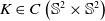 $ K\in C\left ({\mathbb{S}^2}\times {\mathbb{S}^2}\right )$
, invariant under rotations, non-negative and satisfying
$ K\in C\left ({\mathbb{S}^2}\times {\mathbb{S}^2}\right )$
, invariant under rotations, non-negative and satisfying
 \begin{equation*} \displaystyle\int _{\mathbb{S}^2} K(n,n')dn=1 .\end{equation*}
Let $ n,\omega \in {\mathbb{S}^2}$
. Then there exists finitely many
$ n,\omega \in {\mathbb{S}^2}$
. Then there exists finitely many $ n_1,\cdots ,n_N\in {\mathbb{S}^2}$
such that
$ n_1,\cdots ,n_N\in {\mathbb{S}^2}$
such that
 \begin{equation} K(n_{i-1},n_i)\gt 0 \text{ for all }i\in \{1,\cdots ,N+1\}, \end{equation}
where we defined $ n_0=n$
and
$ n_0=n$
and $ n_{N+1}=\omega$
.
$ n_{N+1}=\omega$
.
Proof. Since $ K\geq 0$
but it is not equal zero, there exists a pair
$ K\geq 0$
but it is not equal zero, there exists a pair $ n',n''\in {\mathbb{S}^2}$
such that
$ n',n''\in {\mathbb{S}^2}$
such that $ K(n',n'')\gt 0$
. Hence, applying the rotation
$ K(n',n'')\gt 0$
. Hence, applying the rotation $ {\mathcal{R}}_{n,n'}$
yields the existence of
$ {\mathcal{R}}_{n,n'}$
yields the existence of $ n_*$
such that
$ n_*$
such that $ K(n,n_*)\gt 0$
. By continuity, the set
$ K(n,n_*)\gt 0$
. By continuity, the set $ B_n=\{\tilde {n}\in {\mathbb{S}^2}:K(n,\tilde {n})\gt 0\}$
is open. Hence, there exists
$ B_n=\{\tilde {n}\in {\mathbb{S}^2}:K(n,\tilde {n})\gt 0\}$
is open. Hence, there exists $ \delta \gt 0$
and
$ \delta \gt 0$
and $ n_1\in {\mathbb{S}^2}$
such that
$ n_1\in {\mathbb{S}^2}$
such that $ B_\delta (n_1)\subset B_n$
. We remark that
$ B_\delta (n_1)\subset B_n$
. We remark that $ \delta \gt 0$
is independent of the choice of
$ \delta \gt 0$
is independent of the choice of $ n\in {\mathbb{S}^2}$
. Indeed, for any
$ n\in {\mathbb{S}^2}$
. Indeed, for any $ n'\in {\mathbb{S}^2}$
, there exists some
$ n'\in {\mathbb{S}^2}$
, there exists some $ n''\in {\mathbb{S}^2}$
such that
$ n''\in {\mathbb{S}^2}$
such that $ B_\delta (n'')\subset B_{n'}$
. This is a consequence of the invariance under rotations of
$ B_\delta (n'')\subset B_{n'}$
. This is a consequence of the invariance under rotations of $ K$
. Indeed, it is not difficult to see that
$ K$
. Indeed, it is not difficult to see that $ {\mathcal{R}}_{n,n'}({B_n})= B_{n'}$
and so
$ {\mathcal{R}}_{n,n'}({B_n})= B_{n'}$
and so $ {\mathcal{R}}_{n,n'}(B_\delta (n_1))=B_\delta ({\mathcal{R}}_{n,n'}(n_1))\subset B_{n'}$
.
$ {\mathcal{R}}_{n,n'}(B_\delta (n_1))=B_\delta ({\mathcal{R}}_{n,n'}(n_1))\subset B_{n'}$
.
Let us consider the set
 \begin{equation*} A_n=\{\tilde {n}\in {\mathbb{S}^2}: \text{ there exists }n_1,\cdots ,n_N\in {\mathbb{S}^2} \text{ such that (A.1) holds for }n_0=n \text{ and }n_{N+1}=\tilde {n}\}. \end{equation*}
By the previous consideration, we know that $ A_n$
is not empty. We claim now that
$ A_n$
is not empty. We claim now that $ B_\delta (n')\subset A_n$
for any
$ B_\delta (n')\subset A_n$
for any $ n'\in A_n$
. Indeed, let
$ n'\in A_n$
. Indeed, let $ \delta \gt 0$
as above. Since
$ \delta \gt 0$
as above. Since $ n'\in A_n$
, then
$ n'\in A_n$
, then $ B_{n'}$
is not empty, and there exists some
$ B_{n'}$
is not empty, and there exists some $ n_1\in {\mathbb{S}^2}$
such that
$ n_1\in {\mathbb{S}^2}$
such that $ B_\delta (n_1)\subset B_{n'}$
. It is easy to see that
$ B_\delta (n_1)\subset B_{n'}$
. It is easy to see that $ n_1\in A_n$
. Let now
$ n_1\in A_n$
. Let now $ \tilde {n}\in B_\delta (n')$
, then
$ \tilde {n}\in B_\delta (n')$
, then $ {\mathcal{R}}_{n',n_1}(\tilde {n})\in B_\delta (n_1)$
. Hence,
$ {\mathcal{R}}_{n',n_1}(\tilde {n})\in B_\delta (n_1)$
. Hence, $ K(n',{\mathcal{R}}_{n',n_1}(\tilde {n}))=K(n_1,\tilde {n})\gt 0$
. Since also
$ K(n',{\mathcal{R}}_{n',n_1}(\tilde {n}))=K(n_1,\tilde {n})\gt 0$
. Since also $K(n',n_1)\gt 0$
, we conclude that
$K(n',n_1)\gt 0$
, we conclude that $ B_\delta (n')\subset A_n$
for all
$ B_\delta (n')\subset A_n$
for all $ n'\in A_n$
. Hence,
$ n'\in A_n$
. Hence, $ A_n$
is open, and it is the whole sphere
$ A_n$
is open, and it is the whole sphere $ {\mathbb{S}^2}$
. Indeed, assume
$ {\mathbb{S}^2}$
. Indeed, assume $ A_n \ne {\mathbb{S}^2}$
. Then, since
$ A_n \ne {\mathbb{S}^2}$
. Then, since $ A_n$
is open, the boundary
$ A_n$
is open, the boundary $ \partial A_n=\overline {A}_n\setminus A_n$
is not empty. Let
$ \partial A_n=\overline {A}_n\setminus A_n$
is not empty. Let $ n^*\in \partial A_n$
and let
$ n^*\in \partial A_n$
and let $ n_0\in A_n$
with
$ n_0\in A_n$
with $ d(n^*,n_0)\lt \frac {\delta }{3}$
, where
$ d(n^*,n_0)\lt \frac {\delta }{3}$
, where $ d(n^*,n_0)$
is the distance on
$ d(n^*,n_0)$
is the distance on $ {\mathbb{S}^2}$
between the two points
$ {\mathbb{S}^2}$
between the two points $ n^*,n_0\in {\mathbb{S}^2}$
. Since
$ n^*,n_0\in {\mathbb{S}^2}$
. Since $ n^*\in \partial A_n$
, it is true that
$ n^*\in \partial A_n$
, it is true that
 \begin{equation*} B_{\frac {\delta }{3}}(n^*)\cap A_n \ne \emptyset \text{ and } B_{\frac {\delta }{3}}(n^*)\cap A^c_n \ne \emptyset . \end{equation*}
On the other hand, we know that $ B_\delta (n_0)\subset A_n$
and therefore
$ B_\delta (n_0)\subset A_n$
and therefore
 \begin{equation*} B_{\frac {\delta }{3}}(n^*)\subset B_{\frac {\delta }{2}}(n^*)\subset B_\delta (n_0)\subset A_n. \end{equation*}
This contradiction concludes the proof of LemmaA.1.
Proof of Proposition
2.1. We first show that $ \varphi$
is continuous. Let
$ \varphi$
is continuous. Let $ \varepsilon \gt 0$
. By the continuity of the kernel
$ \varepsilon \gt 0$
. By the continuity of the kernel $ K$
, there exists some
$ K$
, there exists some $ \delta \gt 0$
such that
$ \delta \gt 0$
such that
 \begin{equation*} \left |K(n_1,n_1')-K(n_2,n_2')\right |\lt \frac {\varepsilon }{4\pi \Arrowvert \varphi \Arrowvert _\infty } \end{equation*}
for all $ n_1,n_2,n_1',n_2'\in {\mathbb{S}^2}$
with
$ n_1,n_2,n_1',n_2'\in {\mathbb{S}^2}$
with $ d(n_1,n_2)+d(n_1',n_2')\lt \delta$
. Let hence
$ d(n_1,n_2)+d(n_1',n_2')\lt \delta$
. Let hence $ n_1,n_2\in {\mathbb{S}^2}$
with
$ n_1,n_2\in {\mathbb{S}^2}$
with $ d(n_1,n_2)\lt \delta$
, then it is easy to see that
$ d(n_1,n_2)\lt \delta$
, then it is easy to see that $ \varphi$
is continuous since
$ \varphi$
is continuous since
 \begin{align*} \begin{aligned} \left |\varphi (n_1)-\varphi (n_2)\right |&=\left |H[\varphi ](n_1)-H[\varphi ](n_2)\right |\\[5pt] &\leq \displaystyle\int _{\mathbb{S}^2} \left |K(n_1,n')-K(n_2,n')\right ||\varphi (n')|\;dn'\lt \varepsilon . \end{aligned} \end{align*}
We move now to the proof of claim $ (ii)$
. Let
$ (ii)$
. Let $ M=\max _{n\in {\mathbb{S}^2}}(\varphi (n))$
. By continuity, there exists some
$ M=\max _{n\in {\mathbb{S}^2}}(\varphi (n))$
. By continuity, there exists some $ n_* \in {\mathbb{S}^2}$
such that
$ n_* \in {\mathbb{S}^2}$
such that $ M=\varphi (n_*)$
. We define the set
$ M=\varphi (n_*)$
. We define the set $ A_M=\left \{n\in {\mathbb{S}^2}:\: \varphi (n)=M\right \}$
. Thus,
$ A_M=\left \{n\in {\mathbb{S}^2}:\: \varphi (n)=M\right \}$
. Thus, $ A_M$
is not empty, and by continuity, it is also closed. We claim that
$ A_M$
is not empty, and by continuity, it is also closed. We claim that $ A_M$
is also open, which implies claim
$ A_M$
is also open, which implies claim $ (ii)$
. Let
$ (ii)$
. Let $ n\in A_M$
. Consider
$ n\in A_M$
. Consider $ B_n=\{\tilde {n}\in {\mathbb{S}^2}:K(n,\tilde {n})\gt 0\}$
. Let
$ B_n=\{\tilde {n}\in {\mathbb{S}^2}:K(n,\tilde {n})\gt 0\}$
. Let $ \varepsilon \gt 0$
and
$ \varepsilon \gt 0$
and $ B_n^\varepsilon =\{\tilde {n}\in B_n:\varphi (\tilde {n})\lt M-\varepsilon \}$
. We show
$ B_n^\varepsilon =\{\tilde {n}\in B_n:\varphi (\tilde {n})\lt M-\varepsilon \}$
. We show $\varphi (\tilde {n})=M$
for all
$\varphi (\tilde {n})=M$
for all $ \tilde {n}\in B_n$
. It is easy to see that this is true if
$ \tilde {n}\in B_n$
. It is easy to see that this is true if $ B_n^\varepsilon =\emptyset$
for all
$ B_n^\varepsilon =\emptyset$
for all $ \varepsilon \gt 0$
. If not, let
$ \varepsilon \gt 0$
. If not, let $ \varepsilon \gt 0$
so that
$ \varepsilon \gt 0$
so that $ B_n^\varepsilon \ne \emptyset$
. Then
$ B_n^\varepsilon \ne \emptyset$
. Then
 \begin{align*} \begin{aligned} M=\varphi (n)=\displaystyle\int _{B_n^\varepsilon } K(n,n')\varphi (n')dn'+\displaystyle\int _{\left (B_n^\varepsilon \right )^c} K(n,n')\varphi (n')dn'\lt M-\varepsilon \displaystyle\int _{B_n^\varepsilon } K(n,n')dn'\lt M. \end{aligned} \end{align*}
Arguing as in the proof of LemmaA.1, there exists a $ \delta \gt 0$
such that
$ \delta \gt 0$
such that $ B_\delta (n_0)\subset B_n$
for some
$ B_\delta (n_0)\subset B_n$
for some $ n_0\in B_n$
. Hence, using the same argument, since
$ n_0\in B_n$
. Hence, using the same argument, since $ n_0\in A_M$
, it is also true that
$ n_0\in A_M$
, it is also true that $\varphi (\tilde {n})=M$
for all
$\varphi (\tilde {n})=M$
for all $ \tilde {n}\in B_{n_0}$
. Using the rotation invariance of the kernel analogously as we have done in LemmaA.1, we see that
$ \tilde {n}\in B_{n_0}$
. Using the rotation invariance of the kernel analogously as we have done in LemmaA.1, we see that
 \begin{equation*} {\mathcal{R}}_{n,n_0}\left (B_\delta (n_0)\right )=B_\delta (n)\subset {\mathcal{R}}_{n,n_0}(B_n)=B_{n_0}\subset A_M . \end{equation*}
We have just proved that the closed non-empty set $ A_M$
is open, and hence, it must be the whole sphere
$ A_M$
is open, and hence, it must be the whole sphere $ {\mathbb{S}^2}$
.
$ {\mathbb{S}^2}$
.
Finally, we prove claim $ (iii)$
. To this end, we notice that the linear operator
$ (iii)$
. To this end, we notice that the linear operator $ H$
maps
$ H$
maps $L^p$
-functions to continuous bounded functions. Analogously as in the proof of
$L^p$
-functions to continuous bounded functions. Analogously as in the proof of $ (i)$
, this is a direct consequence of the Hölder inequality and the fact that the scattering kernel
$ (i)$
, this is a direct consequence of the Hölder inequality and the fact that the scattering kernel $ K$
is continuous. Hence,
$ K$
is continuous. Hence, $ (Id-H)_1:L^1({\mathbb{S}^2})\to L^1({\mathbb{S}^2})$
given by
$ (Id-H)_1:L^1({\mathbb{S}^2})\to L^1({\mathbb{S}^2})$
given by $ (Id-H)_1\varphi =\varphi -H[\varphi ]$
is a well-defined operator, which maps integrable functions to integrable functions. Since
$ (Id-H)_1\varphi =\varphi -H[\varphi ]$
is a well-defined operator, which maps integrable functions to integrable functions. Since $ H[\varphi ]\in C({\mathbb{S}^2})$
for any
$ H[\varphi ]\in C({\mathbb{S}^2})$
for any $ \varphi \in L^1({\mathbb{S}^2})$
, if
$ \varphi \in L^1({\mathbb{S}^2})$
, if $ (Id-H)_1\varphi =0$
, then
$ (Id-H)_1\varphi =0$
, then $ (ii)$
also applies and hence
$ (ii)$
also applies and hence $ \varphi =\text{const}$
. This means that the null space of
$ \varphi =\text{const}$
. This means that the null space of $ (Id-H)_1$
as an operator acting on
$ (Id-H)_1$
as an operator acting on $ L^1({\mathbb{S}^2})$
is given by
$ L^1({\mathbb{S}^2})$
is given by
 \begin{equation*}\mathcal{N}\left ((Id-H)_1\right )=\text{span}\langle 1\rangle =\{f=c:\; c\in {\mathbb{R}}\}. \end{equation*}
It is not difficult to see that the dual operator $ (Id-H)_1^*:L^\infty ({\mathbb{S}^2})\to L^\infty ({\mathbb{S}^2})$
is exactly given by
$ (Id-H)_1^*:L^\infty ({\mathbb{S}^2})\to L^\infty ({\mathbb{S}^2})$
is exactly given by $ (Id-H)$
. Indeed, let
$ (Id-H)$
. Indeed, let $ f\in L^1({\mathbb{S}^2})$
and
$ f\in L^1({\mathbb{S}^2})$
and $ g\in L^\infty ({\mathbb{S}^2})$
. We compute using the invariance under rotations of the kernel
$ g\in L^\infty ({\mathbb{S}^2})$
. We compute using the invariance under rotations of the kernel $ K$
$ K$
 \begin{align*} \begin{aligned} \displaystyle\int _{\mathbb{S}^2} dn \;g(Id-H)_1[f]&= \displaystyle\int _{\mathbb{S}^2} dn \;g(n)f(n)- \displaystyle\int _{\mathbb{S}^2} dn\displaystyle\int _{\mathbb{S}^2} dn'\;K(n,n')g(n)f(n')\\[5pt] &=\displaystyle\int _{\mathbb{S}^2} dn\; g(n)f(n)-\displaystyle\int _{\mathbb{S}^2} dn'\displaystyle\int _{\mathbb{S}^2} dn\;K(n',n)g(n)f(n')=\displaystyle\int _{\mathbb{S}^2} dn \;(Id-H)[g]f. \end{aligned} \end{align*}
Therefore, by the orthogonality of the null space to the range of the dual operator, we conclude
 \begin{align*} \begin{aligned} \text{Ran}(Id-H)&=\left \{\varphi \in L^\infty ({\mathbb{S}^2}): \displaystyle\int _{\mathbb{S}^2} \varphi (n)f(n)\;dn=0\; \forall f\in \mathcal{N}\left ((Id-H)_1\right )\right \}\\[5pt] &=\left \{\varphi \in L^\infty ({\mathbb{S}^2}): \displaystyle\int _{\mathbb{S}^2} \varphi (n)\;dn=0\right \}. \end{aligned} \end{align*}
Appendix B Details of the numerical simulation
In Section 7.1, we presented a numerical result for problem (7.1). We now explain the derivation of (7.1) from the stationary problem (1.12), and we present the discretization used in order to solve this problem numerically. For more details about the code, we refer to [Reference Demattè and Velázquez15]. First of all, we assume $ \alpha ^a_\nu =\alpha _\nu ^s=\frac {1}{2}$
; moreover, we set
$ \alpha ^a_\nu =\alpha _\nu ^s=\frac {1}{2}$
; moreover, we set $ \ell _A=\ell _S=\varepsilon$
, and we consider the case of a constant scattering kernel, namely,
$ \ell _A=\ell _S=\varepsilon$
, and we consider the case of a constant scattering kernel, namely, $ K(n,n')=\frac {1}{4\pi }$
.
$ K(n,n')=\frac {1}{4\pi }$
.
Plot of the approximate solution to the problem (7.1), cf. [
Reference Demattè and Velázquez15
]. The blue line represents $ J(x,-0.7)$
, the orange line
$ J(x,-0.7)$
, the orange line $ J(x,-0.2)$
, the green line
$ J(x,-0.2)$
, the green line $ J(x,0.15)$
and finally the red line
$ J(x,0.15)$
and finally the red line $ J(x,0.86)$
. The grey dashed line is
$ J(x,0.86)$
. The grey dashed line is $ x=0.04$
and shows the thickness of the Milne layer, which is, as expected, of the same order of
$ x=0.04$
and shows the thickness of the Milne layer, which is, as expected, of the same order of $ \ell _M=\varepsilon =0.01$
.
$ \ell _M=\varepsilon =0.01$
.
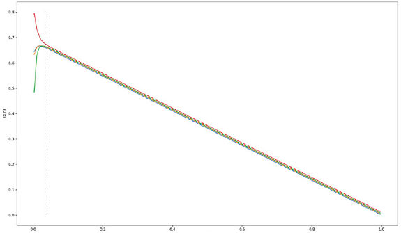
We also consider the domain $ [0,1]\times {\mathbb{R}}^2$
, and we assume that the radiation intensity depends only on the spatial coordinate
$ [0,1]\times {\mathbb{R}}^2$
, and we assume that the radiation intensity depends only on the spatial coordinate $ x_1$
and on the angle between
$ x_1$
and on the angle between $ n\in {\mathbb{S}^2}$
and
$ n\in {\mathbb{S}^2}$
and $ e_1$
. Thus,
$ e_1$
. Thus, $ I_\nu (x,n)=I_\nu (x_1,n_1)$
solves the one-dimensional problem
$ I_\nu (x,n)=I_\nu (x_1,n_1)$
solves the one-dimensional problem
 \begin{equation*} \begin{cases} n_1 \partial _{x_1}I_\nu (x_1,n_1)=\dfrac {1}{2\varepsilon }\left [B_\nu (T(x_1))+\dfrac {1}{2}\displaystyle\int _{-1}^1 I_\nu (x_1,n_1') \ dn_1' -2 I_\nu (x_1,n_1)\right ] & x_1\in (0,1), \ n_1\in [-1,1]\\[5pt] \partial _{x_1}\displaystyle\int _0^\infty \displaystyle\int _{-1}^{1} n_1 I_\nu (x_1,n_1)\ dn_1 \ d\nu =0 & x_1\in (0,1), \ n_1\in [-1,1]\\[5pt] I_\nu (0,n_1)=n_1e^{-\nu }& n_1\gt 0\\[5pt] I_\nu (1,n_1)=0 & n_1\lt 0, \end{cases} \end{equation*}
where we chose as boundary condition at $ x=0$
an anisotropic function and at
$ x=0$
an anisotropic function and at $ x=1$
an isotropic function. Denoting by
$ x=1$
an isotropic function. Denoting by $ (x,n)$
the coordinates
$ (x,n)$
the coordinates $ (x_1,n_1)$
, defining the function
$ (x_1,n_1)$
, defining the function $ J(x,n)=\int _0^\infty I_\nu (x,n) \ d\nu$
, using the divergence-free condition for the flux of radiation and the isotropy of the Planck distribution, we obtain
$ J(x,n)=\int _0^\infty I_\nu (x,n) \ d\nu$
, using the divergence-free condition for the flux of radiation and the isotropy of the Planck distribution, we obtain
 \begin{equation*}2\displaystyle\int _0^\infty B_\nu (T(x)) \ d\nu =\displaystyle\int _{-1}^1 J(x,n) \ dn.\end{equation*}
This implies that $ J(x,n)$
solves (7.1), which is then discretized as follows. Let
$ J(x,n)$
solves (7.1), which is then discretized as follows. Let $ N\gt 0$
. Then, for
$ N\gt 0$
. Then, for $ i,j\in \{0,\ldots ,2N-1\}$
, we define the grid
$ i,j\in \{0,\ldots ,2N-1\}$
, we define the grid
 \begin{align*} x_i=\frac {1+2i}{4N}\in (0,1)\quad \text{ and }\quad n_j=\frac {1+2j}{2N}-1\in (\!-\!1,1). \end{align*}
Hence, according to the upwind scheme, we have to solve the following system of linear equations
 \begin{equation*} \begin{cases} 2Nn_j\left [J(x_{i+1},n_j)-J(x_i,n_j)\right ]-\dfrac {1}{\varepsilon }\left [\dfrac {1}{2N}\sum _{k=0}^{2N-1} J(x_i,n_k)-J(x_i,n_j)\right ]=0& j\lt N, \ i\ne 2N-1,\\[9pt] 2Nn_j\left [J(x_{i},n_j)-J(x_{i-1},n_j)\right ]-\dfrac {1}{\varepsilon }\left [\dfrac {1}{2N}\sum _{k=0}^{2N-1} J(x_i,n_k)-J(x_i,n_j)\right ]=0& j\geq N, \ i\ne 0,\\[9pt] -4Nn_jJ(x_{2N-1},n_j)-\dfrac {1}{\varepsilon }\left [\dfrac {1}{2N}\sum _{k=0}^{2N-1} J(x_{2N-1},n_k)-J(x_{2N-1},n_j)\right ]=0& j\lt N, \ i= 2N-1,\\[9pt] 4Nn_j\left [J(x_0,n_j)-n_j\right ]-\dfrac {1}{\varepsilon }\left [\dfrac {1}{2N}\sum _{k=0}^{2N-1} J(x_0,n_k)-J(x_0,n_j)\right ]=0& j\geq N, \ i= 0, \end{cases} \end{equation*}
where we used $ x_{i+1}-x_i=\frac {1}{2N}$
,
$ x_{i+1}-x_i=\frac {1}{2N}$
, $ n_{j+1}-n_j=\frac {1}{N}$
and the considered boundary conditions. The results represented in Figure 2 were obtained by solving this system with Python for
$ n_{j+1}-n_j=\frac {1}{N}$
and the considered boundary conditions. The results represented in Figure 2 were obtained by solving this system with Python for $ N=70$
and
$ N=70$
and $ \varepsilon =0.01$
and plotting the results obtained for
$ \varepsilon =0.01$
and plotting the results obtained for $ j\in \{20,55,80,130\}$
. Finally, we remark that we observe the formation of a Milne layer only close to
$ j\in \{20,55,80,130\}$
. Finally, we remark that we observe the formation of a Milne layer only close to $ x=0$
since the boundary condition at
$ x=0$
since the boundary condition at $ x=1$
is already isotropic.
$ x=1$
is already isotropic.


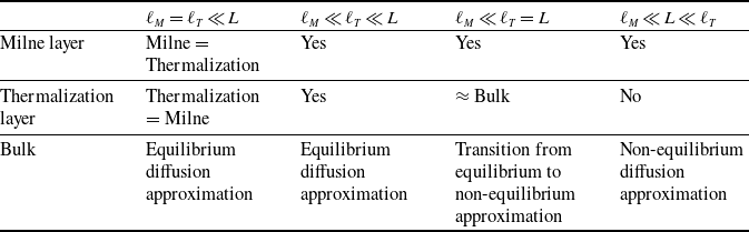
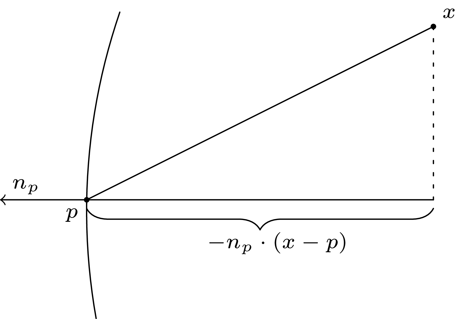
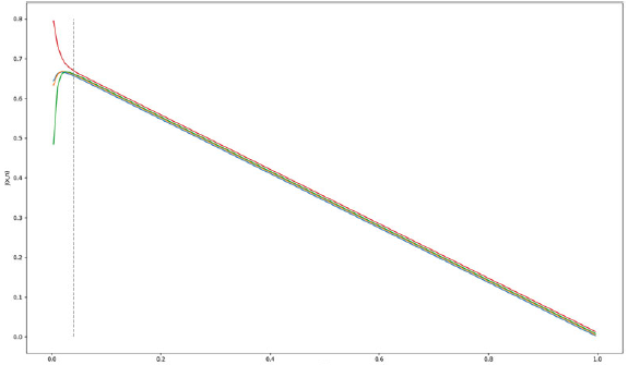
 J(x,−0.7)
 J(x,−0.2)
 J(x,0.15)
 J(x,0.86)
 x=0.04
 ℓM=ε=0.01
 Open access

