


1. Introduction
In many geophysical and cardiovascular flows, and in flows around flying or swimming animals, the turbulent boundary layer (TBL) formed on the surface of an object is subject to a time-varying, non-zero pressure gradient (Li et al. Reference Li, Beech-Brandt, John, Hoskins and Easson2007; Momen & Bou-Zeid Reference Momen and Bou-Zeid2017; Guo et al. Reference Guo, Zhang, Yasuda, Yang, Galipon and Rival2021). Changes in curvature or variation of the freestream pressure distribution might cause the boundary layer to thicken and detach from the surface under the effect of a strong enough deceleration (or adverse pressure gradient, APG). Conversely, the boundary layer may relaminarise under the influence of a strong enough acceleration (or favourable pressure gradient, FPG).
Starting in the 1950s, researchers delved into the physics of separated flows (Schubauer & Klebanoff Reference Schubauer and Klebanoff1951; Stratford Reference Stratford1959; Perry & Fairlie Reference Perry and Fairlie1975; Kline, Bardina & Strawn Reference Kline, Bardina and Strawn1983), yet today answers to key questions related to the physics of separated flows are still missing (Simpson Reference Simpson1989; Weiss, Mohammed-Taifour & Schwaab Reference Weiss, Mohammed-Taifour and Schwaab2015; Mohammed-Taifour & Weiss Reference Mohammed-Taifour and Weiss2016; Wu & Piomelli Reference Wu and Piomelli2018). The picture becomes even more complicated when we consider applications in which pressure gradients are both space- and time-dependent. The time-varying pressure distribution gives rise to transient flow separation, which, in some cases, leads to the advection and shedding of large-scale vortical structures; for instance, in the case of dynamic stall on a pitching airfoil (Simpson Reference Simpson1989; Rival & Tropea Reference Rival and Tropea2010; Williams et al. Reference Williams, An, Iliev, King and Reißner2015). An extensive literature review on the effects of steady (both adverse and favourable) pressure gradients on mean-flow quantities has been presented in Ambrogi, Piomelli & Rival (Reference Ambrogi, Piomelli and Rival2022); the rest of this section will be devoted to the effects of steady and unsteady pressure gradients on higher-order moments. Subsequently, the main objectives of this investigation are described, followed by an outline of the rest of the paper.
1.1. Effects of steady and unsteady pressure gradients on higher-order moments
Our focus here is on pressure-induced separated flows, in which the flow detaches from the wall solely due to the APG. In pressure-induced separated flows the detachment and reattachment locations can fluctuate in space, and the size of the resulting turbulent separation bubble (TSB) will vary. Researchers have characterised the flow in which a separation bubble was formed; Mabey (Reference Mabey1972), for instance, investigated the low-frequency content of wall-pressure fluctuations inside several TSBs in subsonic conditions. The reattachment location played a significant role in the flow dynamic, as it was the region where fluctuation level reached a maximum.
Very common experimental techniques to generate a steady APG-to-FPG distribution on a flat plate involve a suction-only set-up on the top wall of a wind tunnel (Dianat & Castro Reference Dianat and Castro1989, Reference Dianat and Castro1991; Dengel & Fernholz Reference Dengel and Fernholz1990; Alving & Fernholz Reference Alving and Fernholz1996), allowing the boundary layer to detach under the effect of an APG and to naturally reattach to the wall, or a suction–blowing profile that forces the flow to reattach causing a strong FPG. Given the similarity of our computational set-up, the latter case is of more direct interest to the present investigation, and will be discussed in more detail. Patrick (Reference Patrick1985), for instance, carried out an experimental study of a large-scale TSB on a flat plate. The separation region was unstable and characterised by the advection of large eddies downstream. The advection process was found to be the cause of a low-frequency, non-periodic flapping of the reattachment point.
Understanding the unsteady behaviour of the separation region has been the driving objective in the extensive studies carried out by Weiss et al. (Reference Weiss, Mohammed-Taifour and Schwaab2015) and Mohammed-Taifour & Weiss (Reference Mohammed-Taifour and Weiss2016), in which they used particle image velocimetry (PIV) in a massively separated, pressure-induced TSB on a flat plate. They found that the longitudinal turbulence intensity remained nearly constant along the centre of the shear layer and, in line with results shown by the numerical simulation of a TSB of Na & Moin (Reference Na and Moin1998), the Reynolds shear-stress increased and reached a maximum downstream of the reattachment point. Moreover, they found that the streamwise position of the maximum vertical turbulence intensity corresponds to the location of maximum wall-pressure fluctuations.
In their recent work Le Floc'h et al. (Reference Le Floc'h, Weiss, Mohammed-Taifour and Dufresne2020) carried out measurements of wall-pressure and velocity fluctuations for three pressure-induced TSBs of various sizes. In all cases the distribution of wall-pressure fluctuations shows two maxima: the first being close to the location of maximum APG; and the second located at the end of the intermittent backflow region. Distributions of turbulent wall-normal and shear stresses were analysed, and both showed a monotonic increase with the streamwise distance. Although this result is in contrast to previous numerical observations (Na & Moin Reference Na and Moin1998; Wu & Piomelli Reference Wu and Piomelli2018), the authors attributed the cause to the much higher Reynolds number in their test case, and to the weaker transpiration profile.
Over the years, several numerical simulations of boundary layers under steady pressure-gradient distributions were carried out. These studies confirmed behaviours observed experimentally, and explained new features of separated flows. Notable was the investigation carried out by Na & Moin (Reference Na and Moin1998) of a separated TBL on a flat plate at an inflow Reynolds number (based on momentum thickness  $\theta$)
  $Re_{\theta }=300$. The formation of a closed steady TSB was achieved by imposing a suction–blowing vertical velocity profile at the top boundary of the domain. They observed that both detachment and reattachment locations were not fixed in space. Moreover, the instantaneous vorticity showed vortical structures moving away from the wall into the separated shear layer, turning around the bubble and impinging on the wall in the reattachment region. This process caused the location of maximum turbulent intensities to occur in the middle of the shear layer.
Following the approach taken by Na & Moin (Reference Na and Moin1998), Abe (Reference Abe2017) investigated three TSBs over a flat plate for a range of Reynolds number up to  $Re_\theta =900$. The focus was given to the Reynolds-number dependence of fluctuations of the wall pressure (
 $p_w$). The root-mean-square fluctuations of
  $p_w$ showed two peaks, upstream and downstream of the TSB. The author also mentioned an important contribution to
  $p_w$ given by a vertical motion generating negative Reynolds stresses.
In a more recent study, Wu, Meneveau & Mittal (Reference Wu, Meneveau and Mittal2020) performed numerical simulations of a separated TBL on a flat plate using two different transpiration profiles: a suction–blowing profile, consistent with the simulations of Na & Moin (Reference Na and Moin1998) and Abe (Reference Abe2017), and a suction-only profile. This resulted in the generation of two very different separation bubbles; in the suction-only case the TSB was allowed to reattach naturally to the wall. The authors showed that the suction-only profile generated a pressure-gradient and Reynolds-stress distribution in better agreement to separated flows over airfoils and diffusers. Unlike the suction–blowing case, the suction-only case was characterised by a low-frequency unsteadiness (breathing/flapping) in the TSB at a frequency much lower than the dominant high frequency.
The studies mentioned so far focused on steady pressure-gradient distributions; we now shift our attention to unsteady pressure-gradient investigations. We should clarify, as mentioned in Simpson (Reference Simpson1989), that the term unsteady here refers to an organised time-dependent motion, in contrast to the inherently unsteady character of turbulence. Furthermore, our focus will be given to cases in which the unsteadiness is generated by applying a periodic forcing condition on the TBL. The ratio between the convective timescale of the flow, and the unsteady timescale of the perturbation (given by the forcing), is defined by the reduced frequency  $k$, and represents the most important parameter describing the effect of unsteadiness.
Although many researchers, trying to characterise the effect on the flow by introducing a freestream perturbation, have shown that the mean velocity was nearly independent of the reduced frequency  $k$ (Karlsson Reference Karlsson1959; Schachenmann & Rockwell Reference Schachenmann and Rockwell1976; Kenison Reference Kenison1978; Parikh, Reynold & Jayaraman Reference Parikh, Reynold and Jayaraman1982; Simpson, Shivaprasad & Chew Reference Simpson, Shivaprasad and Chew1983; Brereton, Reynolds & Jayaraman Reference Brereton, Reynolds and Jayaraman1990), it was found that as the strength of the APG increased, significant differences arose in the velocity profile as the reduced frequency increased (Covert & Lorber Reference Covert and Lorber1984).
Of particular relevance to the present work is the experimental investigation carried out by Schatzman & Thomas (Reference Schatzman and Thomas2017) of an unsteady APG TBL at a reduced frequency of  $k\approx 0.12$. The authors showed that the locations of the turbulent intensity peaks shift away from the wall, and that the magnitude of the peaks increases as the strength of the APG increases. It was concluded that for a TBL subject to a sufficiently strong APG to cause an inflectional mean (or phase-averaged) velocity profile, the physics must be dominated by the presence of an embedded shear layer associated with the inviscid instability of the outer inflection point. It was also confirmed that the turbulence-intensity peak corresponds to the instantaneous wall-normal location of the outer inflection point.
As discussed in Ambrogi et al. (Reference Ambrogi, Piomelli and Rival2022), the onset of a transient separation process strongly influences the flow in the detachment region. In many cases, the slow-moving fluid region generated by the flow reversal is highly unstable, periodically advected downstream and out of the domain (Mullin, Greated & Grant Reference Mullin, Greated and Grant1980; Simpson Reference Simpson1989; Ambrogi et al. Reference Ambrogi, Piomelli and Rival2022). This particular flow configuration is difficult to achieve via experiments due to the complexity of the boundary conditions, and the required strength of the pressure gradients. However, newly developed experimental facilities are becoming a key source of insights into the physics of TBLs under unsteady pressure gradients (Parthasarathy & Saxton-Fox Reference Parthasarathy and Saxton-Fox2022).
From a numerical point of view, the increasing computational resources available over recent years have made the literature on unsteady pressure-gradient flow simulations grow considerably. The reader is referred to Ambrogi et al. (Reference Ambrogi, Piomelli and Rival2022) for a complete review of past studies. Here we mention the work carried out by Wissink & Rodi (Reference Wissink and Rodi2003) who performed a direct numerical simulation (DNS) of a laminar separation bubble in the presence of an oscillating external flow. The coupled effect of the particular shape of the top boundary of the domain, and the oscillating inflow pressure gradient, caused the flow to separate and reattach to the wall periodically. They showed that when the inflow starts to accelerate, a spanwise roll of turbulent flow is shed from the shear layer, and soon after the remaining separation bubble moves downstream with the turbulent roll. When analysing the time evolution of the fluctuating turbulent kinetic energy (TKE), the authors observed that TKE was produced inside the new separation bubble, after which the TKE grew and simultaneously the structure expanded in the streamwise direction. Eventually, the area of turbulent flow was advected downstream while expanding due to turbulent diffusion. As shown in § 3, the present results are consistent with their findings.
In our recent characterisation of unsteady flow separation in a TBL (Ambrogi et al. Reference Ambrogi, Piomelli and Rival2022), we described how the transient separation process is affected by the reduced frequency  $k$, and shed light into the underlying physical characteristics associated with hysteresis and its effect on the local flow behaviour. We also pointed out commonalities between unsteady separation on a flat plate and the more complex dynamic-stall process on for instance a pitching airfoil; however, only mean and phase-averaged first-order quantities were examined, and many questions concerning the flow dynamics still remained open.
1.2. Objectives and outline
The objective of the present work is to tackle the following questions.
(i) What is the effect of the reduced frequency
 $k$ on TKE and higher-order statistics?
(ii) What is the effect of the periodic washing-out behaviour, observed for
$k=1$, on the flow physics?(iii) What are the causes behind this washing-out behaviour, and why does it happen only for a specific reduced frequency?


The main goal is to expand the analysis carried out in Ambrogi et al. (Reference Ambrogi, Piomelli and Rival2022), to further characterise the unsteady separation process on a turbulent boundary layer and, finally, to shed light into the complexity of such unsteady separated flows. The paper is structured as follows. § 2 describes the numerical methodology, geometry, boundary conditions and simulation parameters. Section 3 contains the body of the work and presents results both for steady and unsteady pressure gradients. Finally, § 4 contains conclusions and highlights key features appropriate for future investigations.
2. Methodology
2.1. Governing equations and numerical method
In large-eddy simulations (LES) the filtered equations of conservation of mass and momentum are solved. They take the form:
 $$\begin{gather} \frac{\partial \bar{u}_i}{\partial x_i}=0, \end{gather}$$
 $$\begin{gather}\frac{\partial\bar{u}_i}{\partial t} + \frac{\partial}{\partial x_j}(\bar{u}_i\bar{u}_j) ={-}\frac{\partial\bar{p}}{\partial x_i} + \nu\nabla^2\bar{u}_i - \frac{\partial \tau_{ij}}{\partial x_j}. \end{gather}$$
Here  $x_1$,
  $x_2$ and
  $x_3$ (or
  $x$,
$x$,  $y$ and
  $z$) are the streamwise, wall-normal and spanwise directions,
  ${\bar {u}}_{i}$ (or
  $\bar {u},~\bar {v},~\bar {w}$) are the filtered velocity components in the coordinate directions and
  $\bar {p}$ is the pressure (divided by the constant density). The divergence of the subfilter-scale stress tensor,
  $\tau _{ij} = \overline {u_i u_j} - \bar {u}_i\bar {u}_j$, appears on the right-hand side of the momentum equation (2.2). In the present study,
  $\tau _{ij}$ is modelled using the Vreman eddy-viscosity model (Vreman Reference Vreman2004). The Reynolds number based on the boundary layer displacement thickness at the inflow
  $\delta _o^*$ and freestream streamwise velocity at the inflow
  $U_o$ is
  $Re_*=1000$. In the following, the overline will be dropped, and
  $u_i,~p$ will be used to represent the filtered velocity and pressure, respectively.
The governing equations (2.1)–(2.2) are discretised using second-order central differences on a staggered grid, and are integrated using a fractional step method (Chorin Reference Chorin1968; Kim & Moin Reference Kim and Moin1985). The spatial discretisation of the convective terms conserves momentum and energy (Morinishi et al. Reference Morinishi, Lund, Vasilyev and Moin1998). All terms are advanced explicitly in time using a three-step, second-order Runge–Kutta method, except for the diffusive term in  $y$, which is advanced implicitly using a second-order Crank–Nicolson method. The Poisson equation is solved directly via Fourier expansions in the spanwise direction (in which the spacing is uniform) followed by a fast cosine-transform in the streamwise direction, and a direct solver for the resulting tridiagonal matrix in the wall-normal direction. The code is parallelised using the message-passing interface (MPI) and has been thoroughly validated and previously applied to similar cases (Keating et al. Reference Keating, Piomelli, Bremhorst and Nešić2004; Yuan & Piomelli Reference Yuan and Piomelli2015; Wu & Piomelli Reference Wu and Piomelli2018).
2.2. Geometry and boundary conditions
Figure 1 shows the computational domain, of dimensions  $L_x \times L_y \times L_z = 600\delta _o^* \times 64\delta _o^*\times 55\delta _o^*$; the black arrow denotes the flow direction. The dimensions of the domain were chosen based on cases studied in the literature; the domain length, in particular, is significantly longer than that used by Na & Moin (Reference Na and Moin1998) and Abe (Reference Abe2017). A length of
  $100\delta _o^*$ was allocated before and after the pressure-gradient region to ensure a relaxation of the boundary layer towards equilibrium in all steady cases. A uniform grid in the streamwise and spanwise directions, and a stretched grid in the wall-normal direction, were employed. A grid-convergence study was performed, which is described in the following. The final grid uses
  $N_x\times N_y\times N_z = 1536\times 192\times 256$ points. In wall units, defined using the friction velocity
  $u_{\tau }$ at the inflow plane, we have
  $\Delta x^+=18.7$,
  $\Delta y^+_{min}=0.7$ and
  $\Delta z^+=10$, all values comparable with DNSs for both APGs (Na & Moin Reference Na and Moin1998) and ZPGs (Spalart Reference Spalart1988; Schlatter & Örlü Reference Schlatter and Örlü2010).
Sketch of the computational domain. A parallel auxiliary simulation is used to generate the inflow boundary condition at the desired  $Re_*$.

Periodic boundary conditions were used in the spanwise direction. The inflow boundary condition was generated using an auxiliary simulation, as proposed by Lund, Wu & Squires (Reference Lund, Wu and Squires1998) (figure 1). The auxiliary simulation uses the recycling/rescaling boundary conditions (also proposed in that paper) in the streamwise direction. A plane at the desired Reynolds number is extracted at each timestep from the auxiliary calculation and interpolated to match the resolution and domain size of the main simulation. A convective boundary condition was prescribed at the outlet (Orlanski Reference Orlanski1976). On the bottom wall, the no-slip boundary condition was applied.
Unsteady flow separation was obtained by imposing a vertical velocity  $V_\infty (x,t)$ at the freestream that changes both in space and time:
 $$\begin{gather} V_\infty (x,t) =V_o(x)\sin\left(2{\rm \pi}\frac{t}{T}\right) \end{gather}$$
 $$\begin{gather}V_o(x) =\alpha \sin\beta(x-x_r)\exp[-\gamma(x-x_r)^2 ]. \end{gather}$$
 In (2.3)  $T$ is the oscillation period, and
  $V_o$ is the streamwise distribution of wall-normal velocity which follows (2.4) and was chosen to match the case studied by Na & Moin (Reference Na and Moin1998). Here
  $\alpha = 1.25 U_o$,
  $\beta =0.012/\delta _o^*$,
  $\gamma =1.4 \times 10^{-4}/(\delta _{o}^* )^2$ and
  $x_{r}/\delta _{o}^* = 320$. The freestream velocity in the streamwise direction,
  $U_\infty$, was obtained by imposing an irrotational condition on the top boundary (Na & Moin Reference Na and Moin1998; Abe Reference Abe2017; Wu & Piomelli Reference Wu and Piomelli2018):
 \begin{equation} \left.\frac{\partial u}{\partial y}\right\vert_{y=L_y} =\frac{{\rm d}V_\infty}{{\rm d} x} ;\quad \left.\frac{\partial w}{\partial y}\right\vert_{y=L_y}=0. \end{equation}
 While a grid-convergence study on first-order statistics was discussed in Ambrogi et al. (Reference Ambrogi, Piomelli and Rival2022), for the purpose of the present investigation, a validation check and a grid-convergence study for the Reynolds stresses have been carried out. Figure 2(a) shows the distribution of the root mean square (r.m.s.) of the streamwise velocity fluctuations  $u_{rms}$, and Reynolds shear stresses
  $-u'v'$ at
  $Re_\theta =1410$ (normalised with the friction velocity
  $u_\tau$). Results agree very well with previous LES and DNS studies (Spalart Reference Spalart1988; Schlatter & Örlü Reference Schlatter and Örlü2010). Figure 2(b) shows the distribution of
  $u_{rms}$, in the most APG case for three streamwise locations, one before the pressure gradient region, one at the centre of the separation bubble, and the last in the reattachment region. The grid mentioned above was compared with a coarser grid using
  $1152\times 129\times 152$ points. The difference between results obtained with the two grids is less than
  $4\,\%$. Other Reynolds stresses were also compared (not shown here) and showed good agreement.
(a) Distribution of streamwise velocity fluctuations, and Reynolds shear stresses at  $Re_\theta =1410$, both normalised with the friction velocity
  $u_\tau$. Red lines denote the
  $1536\times 192\times 256$ grid;
  ${\square }$ Spalart (Reference Spalart1988);
  ${\bullet }$ Schlatter & Örlü (Reference Schlatter and Örlü2010). (b) Distribution of
  $u_{rms}$ in the most APG case for three streamwise locations. Red solid lines denote the
  $1536\times 192\times 256$ grid; blue dashed lines denote the
  $1152\times 129\times 192$ grid.

2.3. Simulation parameters
As mentioned previously, the unsteadiness is generated by oscillating the wall-normal freestream velocity profile  $V_\infty (x,t)$ using a sine function (2.3). Depending on the phase angle
  $\varPhi$, defined as
  $\varPhi =2{\rm \pi} (t+nT)/T$ (with integer
  $n$), the flow will be subject to a different pressure gradient. Starting at phase
  $\varPhi =0^\circ$, for instance, the pressure gradient is nominally zero. As
  $\varPhi$ increases, the flow will move into a region of the cycle (
 $0^\circ < \varPhi < 180^\circ$) in which the freestream velocity
  $U_\infty$ first increases (causing a FPG) and then decreases to its inflow value (causing an APG). The maximum FPG-APG phase is reached at
  $\varPhi =90^\circ$. At
  $\varPhi =180^\circ$ the pressure gradient will once again be zero. The phases between
  $0^\circ <\varPhi <180^\circ$ will be referred to as the ‘acceleration side’ of the cycle. Conversely, when
  $180^\circ <\varPhi <360^\circ$ the flow will be in a region in which
  $U_\infty$ first decreases (APG) and then increases (FPG). In this region, referred to as the ‘separation side’ of the cycle, the flow will separate, and the maximum APG-FPG phase is reached at
  $\varPhi =270^\circ$. For post-processing, the oscillation period was divided into 20 equally spaced phases, and a schematic of the complete process is shown in figure 3 in which the freestream velocity
  $U_\infty$ is plotted for the four main phases of the cycle.
Freestream velocity at four key phases in the cycle. Black arrows denote the variation in phase angle  $\varPhi$, and hence change in pressure gradient.

The key parameter governing the unsteadiness is the frequency at which  $V_\infty$ is modulated. In its non-dimensional form, the reduced frequency is defined here as
 \begin{equation} k=\frac{{\rm \pi} f L_{PG}}{U_{o}}, \end{equation}
where  $f=1/T$ is the imposed frequency,
  $L_{PG}$ is the characteristic length of our flow and
  $U_o$ is the freestream velocity at the inflow plane. We chose
  $L_{PG}$ as the length over which the pressure gradient varies (
 $|V_o|>0.06 \max (|V_o|)$). This decision was justified by a comparison with the more complex physical application of a pitching airfoil where the chord length of the airfoil is used in the reduced frequency definition. In analogy to our case, the chord length of the airfoil represents the region over which the pressure gradient varies.
As pointed out in § 1, the reduced frequency is a standard normalisation used in the unsteady aerodynamic community, and defines the ratio between the convective timescale of the flow and the imposed unsteady timescale. In order to study a wide range of physical behaviours, we performed simulations for  $k=10$,
  $1$ and
  $0.2$. Ambrogi et al. (Reference Ambrogi, Piomelli and Rival2022) showed that in the case
  $k=10$, a case in which the convective timescale of the flow dominates over the unsteady imposed timescale, the flow response is almost synchronised with the freestream forcing except in a very small layer close to the wall in which viscosity generates a small lag. As the frequency decreases the two timescales become comparable and a significant lag in response to the freestream forcing is generated, and at
  $k=1$ the separation region is periodically advected downstream and washed out of the domain. As
  $k$ decreases to
  $k=0.2$, a quasi-steady state is reached and hysteresis effects are confined only to a part of the cycle.
To analyse the results all quantities were first averaged in the homogeneous spanwise direction. Afterwards two averaging procedures were used: time averaging (indicated with an overline) and phase averaging (indicated with angle brackets). The time- and phase-averaging operators are defined respectively as
 \begin{align} \bar{f}(x,y) = \lim_{T\longrightarrow\infty} \frac{1}{T}\int_{0}^{T}f\left(x,y,t\right){\rm d}t; \quad \left\langle\, f\left(x,y,t\right)\right\rangle = \lim_{N\longrightarrow\infty} \frac{1}{N}\sum_{n=0}^{N}f\left(x,y,t+n T\right), \end{align}
where  $T$ represents the oscillation period. We also carried out numerical simulations with a steady pressure gradient corresponding to that imposed at
  $\varPhi =0^\circ$,
  $54^\circ$,
  $90^\circ$,
  $270^\circ$ and
  $306^\circ$. The Reynolds number chosen for the present numerical simulation (
 $Re_{*}=1000$) was consistent with previous investigations (Abe Reference Abe2017; Coleman, Rumsey & Spalart Reference Coleman, Rumsey and Spalart2018). Phase-averaged statistics were accumulated over several periods, dependent on the reduced frequency. To estimate the uncertainty of the results in terms of sample convergence, we compared the phase-averaged velocity obtained by using only half of the cycles with that obtained using all available cycles. For the
  $k=0.2$ case, which is the most critical, since the period is longer and fewer cycles could be computed, the difference in the phase-averaged TKE profiles was less than 3 %, whereas for the other cases it was less than 1 %.
3. Results
3.1. Effects of unsteady separation on Reynolds stresses
In Ambrogi et al. (Reference Ambrogi, Piomelli and Rival2022) we showed how the mean flow is characterised at some frequencies by hysteresis. Hysteresis occurs due to the asymmetry of the flow; before the first ZPG phase,  $270^\circ <\varPhi <360^\circ$, the flow accelerates towards a ZPG behaviour, whereas for
  $90^\circ <\varPhi <180^\circ$ the ZPG behaviour is achieved by flow deceleration. Furthermore, before the first ZPG phase a separated flow is reattaching and returning towards equilibrium, and the footprint of the recirculation is present, and affects the flow greatly, as is shown later. This is particularly significant for
  $k=1$, a case in which the forcing timescale is comparable to the timescale of the mean flow. For the higher frequency the flow does not have the time to adapt to the perturbation in the first place (the recirculation bubble, for instance, is very thin, as shown in figure 9 of that reference). Thus, the recovery to ZPG behaviour is nearly immediate. Conversely, at
  $k=0.2$ the forcing timescale is so large that the flow has more time to recover after maximum APG or FPG (although some asymmetry can still be observed). Note that in both cases the transition from FPG to ZPG is faster than that from APG to ZPG, a consequence of the presence of a recirculation bubble, which alters the flow more significantly than the thinning of the boundary layer caused by the FPG.
Following the same approach, we first compare results for the unsteady pressure-gradient simulations with steady pressure-gradient calculations for the four main phases in the cycle,  $\varPhi =0^\circ$ (ZPG),
  $\varPhi =90^\circ$ (FPG-APG),
  $\varPhi =180^\circ$ (ZPG) and
  $\varPhi =270^\circ$ (APG-FPG), which correspond to previous investigations of steady separated flows (Na & Moin Reference Na and Moin1998; Abe Reference Abe2017; Wu & Piomelli Reference Wu and Piomelli2018).
Profiles of phase-averaged TKE  $\langle \hbox {TKE}\rangle$ are shown in figure 4. For each phase, profiles are extracted at three streamwise locations, one upstream of the pressure-gradient region, one at the centre and the last one downstream of the pressure-gradient region.
Profiles of the phase-averaged TKE  $\langle {\mathrm {TKE}}\rangle$ for four phases in the cycle at three streamwise locations. Comparison is made with steady calculations (symbols) at the same streamwise locations. Profiles are shifted for clarity. From left to right, locations are:
  $x/\delta _o^*=270$,
  $x/\delta _o^*=300$,
  $x/\delta _o^*=450$.
  ${\bullet }$, Steady case; green dotted line,
  $k=10$; blue dash-dotted line,
  $k=1$; orange solid line,
  $k=0.2$.

At high frequency hysteresis effects are restricted to a very thin layer close to the wall where a small lag in response to the freestream forcing is observed (Ambrogi et al. Reference Ambrogi, Piomelli and Rival2022). This effect specifically can be observed at  $\varPhi =0^\circ$ and
  $180^\circ$ where the flow behaves as a canonical ZPG turbulent boundary layer. The low-frequency case (
 $k=0.2$) matches very well the steady calculations at every streamwise location during the two ZPG phases (
 $\varPhi =0^\circ,180^\circ$) and in the acceleration side of the cycle (
 $0^\circ <\varPhi <180^\circ$). A close match persists also at
  $\varPhi =90^\circ$ when the strong APG region causes the peak of
  $\langle \hbox {TKE}\rangle$ to move away from the wall. At
  $\varPhi =270^\circ$ flow separation occurs and, in the
  $k=0.2$ case, a large-scale separation bubble is formed in the centre of the domain. Results for the low-frequency case match reasonably well with the steady calculations in the first two streamwise locations. In agreement with what was observed by Na & Moin (Reference Na and Moin1998), the maximum of
  $\langle \hbox {TKE}\rangle$ occurs above the detachment region and the peak of
  $\langle \hbox {TKE}\rangle$ is now in the middle of the separated shear layer. Further downstream (
 $x/\delta _o^*=450$) the presence of the familiar near-wall peak of
  $\langle \hbox {TKE}\rangle$ implies that the boundary layer is redeveloping towards an equilibrium state; however, for the steady calculation, a second peak of
  $\langle \hbox {TKE}\rangle$ is present, suggesting that the recovery is much faster in the unsteady case. The intermediate frequency case (
 $k=1$) shows an overall similar behaviour, with the difference that in this case the separation bubble at
  $\varPhi =270^\circ$ is much thinner in the wall-normal direction (Ambrogi et al. Reference Ambrogi, Piomelli and Rival2022). As mentioned earlier, the combination of the asymmetry of the flow and the mismatch between forcing and response timescales causes the differences between the two ZPG phases (
 $\varPhi =0^\circ$, and
  $\varPhi =180^\circ$), which are characterised by the same freestream pressure-gradient distribution.
Figure 5 shows phase-averaged Reynolds shear stresses  $-\langle u'v' \rangle$ for the same four phases and streamwise locations. Once again, we observe that the high-frequency case resembles a ZPG boundary layer throughout the cycle. The low-frequency case matches very well the steady calculations in the acceleration side of the cycle. The intermediate frequency case, on the other hand, displays hysteresis effects, evident at the two ZPG phases, but present at other phases also, in line with previous observations. Previous studies showed that the maximum of
  $-\langle u'v'\rangle$ occurs downstream of reattachment (Na & Moin Reference Na and Moin1998; Abe Reference Abe2017; Weiss et al. Reference Weiss, Mohammed-Taifour and Schwaab2015), and that local maxima of the Reynolds shear stresses are reduced significantly in the separation region. This result is observed in the steady calculations (black dots in figure 5); however, unsteady calculations show a different trend. There, in fact, the peak of
  $-\langle u'v'\rangle$ in the reattachment location is significantly suppressed at both frequencies. The high-frequency case does not deviate significantly from the ZPG behaviour, and will not be considered further.
Phase-averaged Reynolds shear stress  $-\langle u'v'\rangle$ profiles for four phases in the cycle and for two reduced frequencies (colours) and streamwise locations (line styles). Comparison is made with steady calculations (symbols) at the same streamwise locations. Profiles are shifted for clarity. From left to right, locations are:
  $x/\delta _o^*=270$,
  $x/\delta _o^*=300$,
  $x/\delta _o^*=450$.
  ${\bullet }$ Steady case; green dotted line,
  $k=10$; blue dash-dotted line,
  $k=1$; orange solid line,
  $k=0.2$.

To establish a connection to our previous investigation (Ambrogi et al. Reference Ambrogi, Piomelli and Rival2022), we have compared the time evolution of TKE with the time evolution of the streamwise velocity ( $\langle u\rangle$) for both frequencies. At the intermediate frequency,
  $k=1$, shown in figure 6, the stalled fluid generated by the flow reversal is advected downstream and is periodically washed out of the domain. This behaviour is consistent with previous experiments on pulsating flows over a backward-facing step (Mullin et al. Reference Mullin, Greated and Grant1980), and stalled flows in diffusers (Simpson Reference Simpson1989). The slow-moving fluid region possesses a very high TKE content, and we observe that contours of high TKE (red lines in figure 6) coincide with the stalled-fluid region and TKE is advected downstream at the same rate.
Contours of phase-averaged streamwise velocity  $\langle u\rangle$ for
  $k=1$, with overlapped contour lines of phase-averaged TKE normalised using the freestream velocity at the inlet
  $U_o$. Only the four key phases of the cycle are shown. Contour levels for TKE are 0.01, 0.05, 0.1 and 0.15.

As the reduced frequency is decreased (figure 7), the separation bubble has now comparable dimensions (both height and length) with the steady calculation. Given the much longer period of the freestream oscillation, the flow has more time to adjust to the freestream forcing, and the separation region appears to be more stable. An evident advection mechanism of  $\langle u\rangle$ or TKE seems absent, but we show, momentarily, that this is not the case.
Contours of phase-averaged streamwise velocity  $\langle u\rangle$ for
  $k=0.2$, with overlapping contour lines of phase-averaged TKE normalised using the freestream velocity at the inlet
  $U_o$. Only the four key phases of the cycle are shown. Contour levels for TKE are 0.01, 0.05, 0.1 and 0.15.

3.2. Advection dynamics
As mentioned in § 2, the cycle was divided into 20 equally spaced phases. Figure 8 shows the phase angle; colours are used as an aid to visualise the sign of the freestream forcing and its temporal characteristics. Starting at  $\varPhi =0^\circ$ (the ZPG phase), the flow moves into the acceleration side of the cycle (coloured in red), which contains all phases in which
  $U_\infty \geqslant 1$. At
  $\varPhi =180^\circ$ the flow is back to a ZPG turbulent boundary layer and, as
  $\varPhi$ increases, the flow enters the separation side of the cycle (coloured blue) containing all phases in which
  $U_\infty \leqslant 1$. The flow separates at
  $\varPhi \approx 270^\circ$. We denote the region of the cycle
  $270^\circ <\varPhi <90^\circ$ the washout region (black dashed rectangle in figure 8), in which the advection and subsequent washout of the stalled fluid and high-TKE regions take place.
Schematic of key phases of a cycle. Represented in red is the acceleration region of the cycle where the FPG precedes the APG and  $U_\infty >1$. Represented in blue is the separation side of the cycle where the APG precedes the FPG and
  $U_\infty <1$. The black dashed rectangle represents the washout region of the cycle where the advection process of TKE is observed.

Figure 9 shows contours of TKE for 11 equispaced phases between the maximum APG-FPG ( $\varPhi =270^\circ$) and the maximum FPG-APG (
 $\varPhi =90^\circ$), for
  $k=1$ (a–k) and
  $k=0.2$ (l–v). Axis colours follow the schematic in figure 8. The same quantity is also shown for the steady case, at the freestream pressure distribution corresponding to
  $\varPhi =270^\circ$ (panel w in figure 9). The same analysis in animation form can be seen in the supplementary movie 1 available at https://doi.org/10.1017/jfm.2023.690.
Contours of phase-averaged TKE for  $k=1$ (a–k) and
  $k=0.2$ (l–v): (a,l)
  $\varPhi =270^\circ$; (b,m)
  $\varPhi =288^\circ$; (c,n)
  $\varPhi =306^\circ$; (d,o)
  $\varPhi =324^\circ$; (e,p)
  $\varPhi =342^\circ$; ( f,q)
  $\varPhi =360^\circ =0^\circ$; (g,r)
  $\varPhi =18^\circ$; (h,s)
  $\varPhi =36^\circ$; (i,t)
  $\varPhi =54^\circ$; (j,u)
  $\varPhi =72^\circ$; (k,v)
  $\varPhi =90^\circ$; (w) steady case, pressure gradient corresponding to
  $\varPhi =270^\circ$. Axis colours follow the convention of figure 8. The solid red line indicates the domain centreline.

We first note (figure 9l–v) that an advection-like phenomenon of TKE plays a significant role also at the lower frequency ( $k=0.2$). At phase
  $\varPhi =270^\circ$, flow separation is extensive and, in line with previous observations, the high-TKE region corresponds to the separated shear layer. This high-TKE region grows and shrinks in the wall-normal direction, but it does not move in space. At phase
  $\varPhi =288^\circ$, with a lag of about
  $18^\circ$ with respect to the freestream forcing, contours of TKE start to resemble figure 9(w) (the steady calculation). Here, the high-TKE region due to the blowing section of the
  $V_\infty$ appears downstream of the separation bubble. Important to note is that, at this frequency, the advection process of TKE takes place in the separation side of the cycle before the freestream forcing changes sign (at
  $\varPhi =0^\circ$, figure 9q).
For the  $k=1$ case, on the other hand, the recirculation bubble is much thinner than in the steady case, and the shear layer separates at a narrower angle and is shorter. As a consequence, the TKE (which is maximum in the shear layer due to its instability) does not reach the same level. In addition to the lower levels of TKE due to the different shape of the recirculation bubble, the high-TKE region in the reattachment location is completely absent. This is due to the fact that (because of the thinness of the recirculation region) the turbulent eddies formed in the shear layer do not impinge on the wall, but rather glance over it. The recirculation bubble grows during the deceleration side of the cycle (figure 9(a–e),
  $270^\circ <\varPhi <360^\circ$). Consequently, the high-TKE region due to the separated shear-layer grows in the wall-normal direction in the separation side of the cycle (
 $270^\circ <\varPhi <342^\circ$). Then, as the freestream forcing changes sign at
  $\varPhi =0^\circ$, the recirculation region is advected downstream, as discussed momentarily, and the high-TKE region moves together with the stalled fluid.
These phenomena can be explained by following the trajectories of fluid particles. We define the ‘phase-averaged particle-paths’ as the trajectories of fluid particles in the phase-averaged velocity field:
 \begin{equation}
\frac{{\rm d}\langle
\boldsymbol{x}_{p}(t)\rangle}{{\rm d}t}
=\langle \boldsymbol{V}(\boldsymbol{x}_{p},t)\rangle; \quad \boldsymbol{x}_{p}\big|_{t=0} =
\boldsymbol{x}_{p,o}, \end{equation}
\begin{equation}
\frac{{\rm d}\langle
\boldsymbol{x}_{p}(t)\rangle}{{\rm d}t}
=\langle \boldsymbol{V}(\boldsymbol{x}_{p},t)\rangle; \quad \boldsymbol{x}_{p}\big|_{t=0} =
\boldsymbol{x}_{p,o}, \end{equation}
where  $\boldsymbol {x}_p$ is the particle position as a function of time and
  $\boldsymbol {x}_{p,o}$ is the initial position. At
  $\varPhi =270^\circ$ tracer particles are introduced in the recirculation bubble, and their motion is followed in time.
Figure 10 shows the trajectory of a rake of 8 particles introduced in the separation zone at  $\varPhi =270^\circ$. The particles are equally spaced in the wall-normal direction in the range
  $1< y/\delta _o^*<15$ (see supplementary movie 2). For
  $k=1$ all the particles initially move upwards, as they are released in the region where the top of the domain is in suction. Outer-layer particles travel more quickly and enter the region where
  $V_\infty <0$ (panel d,
  $\varPhi =324^\circ$) at which point they start moving towards the wall. They impinge on the wall at
  $\varPhi \simeq 0^\circ \unicode{x2013}18^\circ$ (at a shallow angle) so that energy is not transferred from the streamwise Reynolds stress to the other two components, as would be the case in a steady flow. By the time the forcing changes sign (panel f,
  $\varPhi =360^\circ$) they have travelled beyond the region where suction is applied and are not affected by the suction portion of
  $V_\infty$; thus, the outer-layer particles continue their motion parallel to the wall. After maximum acceleration the recirculation bubble shrinks and disappears. The entire region of stalled fluid then begins to be advected downstream (panel f,
  $\varPhi =0^\circ$). This dynamic process is reflected in the acceleration of the near-wall particles (orange and green) that begins at this phase.
Contours of phase-averaged TKE (grayscale) and wall-normal velocity (colour) and particle pathlines for (a–k)  $k=1$ and (l–v)
  $k=0.2$: (a,l)
  $\varPhi =270^\circ$; (b,m)
  $\varPhi =288^\circ$; (c,n)
  $\varPhi =306^\circ$; (d,o)
  $\varPhi =324^\circ$; (e,p)
  $\varPhi =342^\circ$; ( f,q)
  $\varPhi =360^\circ =0^\circ$; (g,r)
  $\varPhi =18^\circ$; (h,s)
  $\varPhi =36^\circ$; (i,t)
  $\varPhi =54^\circ$; (j,u)
  $\varPhi =72^\circ$; (k,v)
  $\varPhi =90^\circ$; pathlines are coloured based on their distance from the wall. Axis colours follow the convention of figure 8.

Unlike the steady or quasi-steady cases, the TKE levels at the reattachment point are not significant, and the only regions with a high TKE content are the incoming boundary layer and the separated shear layer. For  $\varPhi >0^\circ$ the near-wall particles are in the region where
  $V_\infty >0$, and these fluid particles start moving upwards towards the middle of the high-TKE region. Since these particles were originally released in the near-wall region or in the separated shear layer, they have comparatively more TKE than the outer-layer particles. We can speculate that the high-TKE region associated with the recirculation bubble continuously extracts energy from the surroundings, which allows the high-TKE region to maintain a rotational motion (which will be shown momentarily), as well as a constant shape.
For  $k=0.2$ the dynamics are quite different: in addition to the high-TKE region in the separated shear layer, there is a second high-TKE region in the reattachment zone. As discussed earlier, this is similar to what occurs in the steady case. In steady flow the reattachment line is statistically stationary, so that the eddies separating from the wall always reimpinge on it near the average reattachment line. At this frequency, in addition to the unsteadiness due to turbulence, the reattachment line moves forward and backward depending on the size of the recirculation bubble (i.e. on the phase). Furthermore, as shown by the particle pathlines in figure 10, fluid particles that separate at
  $\varPhi =270^\circ$ do not reach the reattachment point until
  $\varPhi =306^\circ$. This behaviour explains the lag between the formation of the separated shear layer and the formation of a high-TKE region near the reattachment point. For
  $\varPhi >306^\circ$ the particles reaching the reattachment point come from a shrinking recirculation bubble, and their impingement plays a lesser role; the high-TKE region formed at earlier phases is not fed by incoming eddies any longer, and is instead advected downstream and washed out of the domain. This phenomenon takes place earlier in the cycle than the washout of the recirculation bubble observed for the intermediate frequency (figure 9). Advection of the stalled fluid from the recirculation bubble is also observed. Similar to the
  $k=1$ case, figure 9(s–v), although is much less evident than at
  $k=1$. Because of the longer period particles released at
  $\varPhi =270^\circ$ have already left the domain when the forcing changes sign; their trajectories, therefore, are determined by the suction–blowing pattern at the release time only; as a consequence, their paths are very similar to the streamlines, another consequence of the quasi-steady nature of this case.
To further analyse the underlying physical mechanisms behind the advection of TKE, figure 11 shows the phase-averaged spanwise vorticity  $\langle \omega _z \rangle = \epsilon _{3jk}\partial \langle u_k\rangle /\partial x_j$ (also shown in supplementary movie 3 in comparison with TKE and relative particle paths). In both cases the recirculation bubble is associated with high vorticity, as is the separated shear layer. While the former is associated with a vortical motion (as will be shown shortly), the vorticity in the shear layer is due to shear only. At the intermediate frequency (
 $k=1$) the rotational vorticity from the recirculation zone is advected out of the domain while maintaining its shape. At the lower frequency (
 $k=0.2$), on the other hand, the rotational vortical region is dissipated much more rapidly, and only the shear-dominated vorticity in the boundary layer remains.
Contours of phase-averaged spanwise vorticity for  $k=1$ (a–k) and
  $k=0.2$ (l–v): (a,l)
  $\varPhi =270^\circ$; (b,m)
  $\varPhi =288^\circ$; (c,n)
  $\varPhi =306^\circ$; (d,o)
  $\varPhi =324^\circ$; (e,p)
  $\varPhi =342^\circ$; ( f,q)
  $\varPhi =360^\circ =0^\circ$; (g,r)
  $\varPhi =18^\circ$; (h,s)
  $\varPhi =36^\circ$; (i,t)
  $\varPhi =54^\circ$; (j,u)
  $\varPhi =72^\circ$; (k,v)
  $\varPhi =90^\circ$; (w) steady case, pressure gradient corresponding to
  $\varPhi =270^\circ$. Axis colours follow the convention of figure 8. The solid red line indicates the domain centreline.

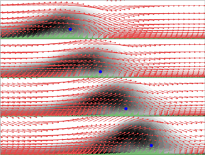
To further investigate these phenomena, we show in figure 12 the TKE contours at the four phases in figure 9( f–i). The vectors are proportional to the velocity in a frame of reference moving at the convection speed of the structure itself,  $\langle u_r \rangle = \langle u \rangle -U_s$. The convection velocity can be measured from the TKE contours in
  $x-\varPhi$ space shown in figure 13; the slope of the high-TKE region is the advection speed,
  $U_s=0.6 U_o$. This slope is nearly constant with
  $y$.
$y$.
Contours of phase-averaged TKE for four consecutive phases,  $k=1$: (a)
  $\varPhi =0^\circ$; (b)
  $\varPhi =18^\circ$; (c)
  $\varPhi =36^\circ$; and (d)
  $\varPhi =54^\circ$. Arrows show the relative velocity on a frame of reference that moves with the structure. Red and green vectors are oriented upstream and downstream, respectively. The blue dot indicates the approximate position of the centre of the vortical structure. The solid blue line indicates the domain centreline.

Contours of phase-averaged TKE as a function of the streamwise direction  $x$ and phase
  $\varPhi$ for the
  $k=1$ case. Three wall-normal positions are shown:
  $y/\delta _{o}^{*}=20$ (a);
  $y/\delta _{o}^{*}=5$ (b); and
  $y/\delta _{o}^{*}=1$ (c).

The use of the relative velocity highlights the vortical nature of the structure being advected. The stalled fluid originates in the recirculation zone (where it has a rotational motion). As the stalled-fluid region is advected downstream, the near-wall flow changes direction but, relative to the advection velocity, the rotational motion is maintained. The high-TKE region is immediately upstream and above the vortical structure (as is the case for the recirculation bubble), and the centre of the vortical structure remains at roughly the same distance from the wall. The solid-body-like advection of the stalled fluid occurs, on this scale, only when the timescale of the flow and that of the forcing are of the same order.
The advection of a strong coherent structure, as described previously, can be treated as an analogue to the dynamic-stall phenomenon observed in unsteady aerodynamics, e.g.leading-edge vortex (LEV) formation on pitching airfoils (see Leishman Reference Leishman2006). Although the source of vorticity forming an LEV emanates from the airfoil surface and/or the leading edge, and as such there are limits in this comparison, the general dynamics of this process are qualitatively the same. In this study we refrain from drawing conclusions regarding these complex vortex–wall interactions observed in unsteady aerodynamics; however, we do expect that the current data and analysis will prove fruitful in future interpretation of dynamic stall, LEV formation and the evolution of vorticity in said unsteady problems.
Although a similar (albeit weaker) advection phenomenon was observed at  $k=0.2$, it does not appear to be associated with a vortical motion. The
  $x$–
$x$– $\varPhi$ plot equivalent to figure 13 does not show a clear footprint of the advection velocity. Following the analysis of figure 12, figure 14 shows TKE contours for the
  $k=0.2$ case overlapped with the relative velocity field generated using
  $U_s=0.6 U_o$. We have tried values of
  $U_s$ between
  $0.2$ and
  $0.8U_o$, and have obtained similar results. At this frequency, the flow is shear-dominated, and a coherent vortical structure cannot be observed during the acceleration phase.
Contours of phase-averaged TKE for four phases,  $k=0.2$: (a)
  $\varPhi =0^\circ$; (b)
  $\varPhi =18^\circ$; (c)
  $\varPhi =36^\circ$; and (d)
  $\varPhi =54^\circ$. Arrows show the relative velocity on a frame of reference that moves with the structure. Red and green vectors are oriented upstream and downstream, respectively. The solid blue line indicates the domain centreline.

The advection of high-TKE regions is an important feature at both frequencies. The high-TKE regions are caused by the instability of the separated shear layer, and represent, therefore, the response of the outer layer to the forcing, i.e. to the changing freestream pressure gradient. To study the response of the inner layer we show, in figure 15, contours of streamwise velocity fluctuations  $u'=u-\langle u\rangle$ in a plane parallel to the wall, at
  $y/\delta _o^*\approx 0.24$, corresponding to
  $y^+=12$ in the ZPG region, during the same 11 phases considered previously.
Contours of instantaneous streamwise velocity fluctuations for  $k=1$ (a–k) and
  $k=0.2$ (l–v) at
  $y^+=12$: (a,l)
  $\varPhi =270^\circ$; (b,m)
  $\varPhi =288^\circ$; (c,n)
  $\varPhi =306^\circ$; (d,o)
  $\varPhi =324^\circ$; (e,p)
  $\varPhi =342^\circ$; ( f,q)
  $\varPhi =360^\circ =0^\circ$; (g,r)
  $\varPhi =18^\circ$; (h,s)
  $\varPhi =36^\circ$; (i,t)
  $\varPhi =54^\circ$; (j,u)
  $\varPhi =72^\circ$; (k,v)
  $\varPhi =90^\circ$; (w) steady case with pressure gradient corresponding to
  $\varPhi =270^\circ$. Axis colours follow the convention of figure 8. For clarity, only half of the domain in the spanwise direction is shown and axis are not equal. The solid red line indicates the domain centreline.

In both cases we observe a standard boundary-layer behaviour, with alternating high- and low-speed streaks in the ZPG region. The streaky structures disappear in the recirculation region (Na & Moin Reference Na and Moin1998; Wu & Piomelli Reference Wu and Piomelli2018), and reappear (with a larger scale) at the reattachment point. This result is consistent with previous experimental and numerical observations that reported that the streak spacing is a function of the pressure gradient and increases by almost an order of magnitude after detachment (Robinson Reference Robinson1991). Post-detachment streaks are very large when the recirculation bubble is largest and, for  $k=0.2$, the impinging eddies result in spanwise oriented structures (Na & Moin Reference Na and Moin1998). In both cases, during the acceleration part of the cycle, the streaks become more elongated in the upstream section (upstream of the red line that indicates the point where the pressure gradient changes sign), and the range of the fluctuations increases, a consequence of the increased Reynolds number (figures 15i–k and 15t–v), see Piomelli, Balaras & Pascarelli (Reference Piomelli, Balaras and Pascarelli2000) and Piomelli & Yuan (Reference Piomelli and Yuan2013). Note also that at
  $\varPhi =90^\circ$ the APG is as strong as that at
  $\varPhi =270^\circ$, but the flow does not separate. This is due to the fact that the FPG in the upstream region gives the flow enough energy to resist separation. During the acceleration side of the cycle the inner layer lags behind the forcing: the velocity fluctuations are largest when
 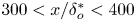 $300< x/\delta ^*_o<400$, where the pressure gradient has already changed sign from FPG to APG. Note also that, while for
  $k=0.2$ a region of higher velocity is formed in the region
  $300< x/\delta ^*_o<400$ immediately after
  $V_\infty$ becomes negative there (panel r,
  $\varPhi =18^\circ$), in the
  $k=1$ case this does not happen until the region of stalled fluid has passed (panel i,
  $\varPhi =54^\circ$). The slow-moving fluid (with high TKE content) acts as a shelter for the near-wall fluid. As the high TKE moves downstream, the near-wall fluid changes under the effect of the pressure gradient, elongated streaks start to form (figure 15h), and from this point, the blowing portion of
  $V_\infty$ is what pushes the high-TKE region out of the domain. Moreover, the spanwise spacing
  $\lambda _z$ of post-detachment streaks is much smaller when compared to
  $k=0.2$, and remains constant throughout this dynamic process.
4. Conclusions
Wall-resolved LES have been carried out to characterise the unsteady separation process on a flat-plate turbulent boundary layer. The oscillating APG and FPG generated by a space- and time-dependent, wall-normal, freestream-velocity profile on the top boundary caused the flow to detach and reattach to the wall periodically. We have analysed the effects of unsteady separation on Reynolds stresses and on the flow topology. In particular, we have focused on the instability of the recirculation region that had been previously observed by several researchers in experimental (Mullin et al. Reference Mullin, Greated and Grant1980; Simpson Reference Simpson1989) and numerical (Ambrogi et al. Reference Ambrogi, Piomelli and Rival2022; Wissink & Rodi Reference Wissink and Rodi2003) studies.
The TKE and Reynolds-stress profiles have demonstrated that the low-frequency case matches very well the steady calculations. Due to the strong APG in the separation region, the peak of the TKE moves away from the wall to the centre of the separated shear layer (Na & Moin Reference Na and Moin1998; Abe Reference Abe2017; Wu & Piomelli Reference Wu and Piomelli2018). However, in the unsteady cases, the reattachment region is quite different from that of the steady flow, as the well-known peak of  $-\langle u'v'\rangle$ observed in previous studies is suppressed. At low frequency, this behaviour is due to a small lag between the response of the velocity and Reynolds stresses and the freestream forcing, which causes the high-TKE region in the reattachment location (due to flow impingement on the wall) to form after the maximum APG phase. At the intermediate frequency, however, the high-TKE region near the reattachment is absent for the entire acceleration region of the cycle. This is due to the fact that (because of the thin recirculation region) the turbulent eddies formed in the shear layer do not impinge on the wall, but rather glance over it.
By analysing the time evolution of TKE in what we defined as the washout region of the cycle ( $\varPhi =270^\circ$ to
  $\varPhi =90^\circ$), we first observed that in both cases a high-TKE region is formed due to the separated shear layer at
  $\varPhi =270^\circ$. The high-TKE region then grows in the wall-normal direction and is subsequently advected downstream and out of the domain. An advection-like phenomenon of TKE is also present at the low frequency (
 $k=0.2$); however, its dynamic behaviour is completely different than that at the intermediate-frequency case (
 $k=1$). For
  $k=1$, the high-TKE region generated by the separated shear-layer grows in the wall-normal direction in the separation side of the cycle, but this shear layer does not start moving until the freestream condition changes sign (
 $\varPhi =0^\circ$), at which point the high-TKE region is advected downstream while keeping a constant shape. For
  $k=0.2$, on the other hand, the region of high TKE formed at the reattachment point is quickly dissipated and advected out of the domain before the freestream forcing changes sign.
The advecting structure, in the  $k=1$ case, is rotational in nature: when seen in a frame of reference moving with the structure itself, this structure resembles the recirculation bubble. The high-TKE region is immediately upstream and above this region, in the same relation to the advecting structure as the separating shear layer is to the recirculation zone. The advection speed was evaluated by examining TKE as a function of the streamwise direction and phase, which displays a constant slope independent of the wall-normal position. The value thus obtained,
  $u_s=0.6\, U_\infty$, is consistent with those reported in the literature for stalled diffusers and dynamic stall over airfoils (Simpson Reference Simpson1989; Leishman Reference Leishman2006). In the low-frequency case, however, no such vortical structure was observed.
To explain why the dynamic process of TKE advection is so different between  $k=1$ and
  $k=0.2$, we have analysed phase-averaged particle pathlines. After seeding an initial set of particles inside the separation region at a fixed streamwise location, and at several wall-normal positions, we observed the particle behaviour during the advection process. At the lower frequency, pathlines behave like streamlines (reinforcing the conclusion that this frequency has reached a quasi-steady state), and are synchronised with the freestream forcing;in the region where
  $V_\infty >0$ the suction causes an upward motion of particles, whereas where
  $V_\infty >0$ the blowing induces a downward motion of the particles. Most importantly, the particles are all advected out of the domain before the wall-normal freestream condition changes from suction–blowing to blowing–suction (around phase
  $\varPhi =0^\circ$ of the cycle). As the frequency was increased, particle pathlines started moving in agreement with the freestream forcing, with upward and downward particle motions corresponding to the freestream suction and blowing. However, given the shorter period of the oscillation, when the freestream condition changes sign, the particles injected at
  $\varPhi =270^\circ$ were still found in the domain. From phase
  $\varPhi =0^\circ$, the particle response to the freestream forcing depends on their wall-normal position. At the lower frequency (
 $k=1$), the set of particles fast enough to escape the effect of the wall were still relatively slow, since they originated in the recirculation region. These particles felt the change in the freestream forcing immediately, were picked up, and started moving downstream inside the advecting high-TKE region. Therefore, the high-TKE region, for the case
  $k=1$, extracts energy from the surrounding fluid while moving downstream, thus maintaining a constant shape.
The present work has related the effects of reduced frequency on the Reynolds stresses, and has clarified the dynamics of the advection of the slow-moving flow observed for  $k=1$. However, additional physical features have been observed, and will be the object of future study. Ongoing work includes an analysis of turbulent structures and their dependence on the reduced frequency. Furthermore, from an engineering point of view, interest lies in practical turbulence modelling, and its capability to deal with unsteady separated flows. The present data can be used to test and validate turbulence models for the Reynolds-averaged Navier–Stokes equations.
Supplementary movies
Supplementary movies are available at https://doi.org/10.1017/jfm.2023.690.
Funding
The authors acknowledge the financial support by the Natural Sciences and Engineering Research Council of Canada (NSERC-CRNSG) under the Discovery Grant programme. This research was enabled in part by computational support provided by the Digital Research Alliance of Canada.
Declaration of interests
The authors report no conflict of interest.


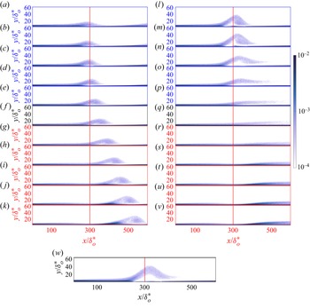


 Open access