


Introduction
Radar sensors are considered a key element of a modern advanced driver assistance system (ADAS), enabling comfort- and safety-related driving features [Reference Rasshofer and Gresser1, Reference Gerstmair, Melzer, Onic and Huemer2]. Their advancement in terms of cost-effectiveness is expected to result in an increasing amount of radar sensors on the road. However, their widespread deployment also implies a rising probability of mutual interference between radar sensors. This is particularly the case for radar sensors mounted to different vehicles [Reference Kunert3], as exemplified in fig. 1(a). Such interference may severely degrade radar system performance, including the introduction of ghost targets or even missing targets [Reference Kim, Mun and Lee4]. Therefore, a variety of potential countermeasures have been developed over the past [Reference Toth, Meissner, Melzer and Witrisal5], which often belong to the categories of detect-and-mitigate or detect-and-avoid [Reference Umehira, Okuda, Wang, Takeda and Kuroda6, Reference Bechter, Sippel and Waldschmidt7]. Moreover, since many of the currently operating automotive radar sensors use the frequency-modulated continuous-wave (FMCW) principle [Reference Patole, Torlak, Wang and Ali8], so are the countermeasures often tailored to handle interference between FMCW radar sensors.
An exemplary traffic scenario in which the blue car receives interfering radar signals originating from the red car. The signals may travel via multiple signal propagation paths, either direct and/or indirect. (a) Without countermeasures: Degradation of radar performance. Targets may be missed and ghost targets may occur. (b) Detect-and-exploit countermeasure: Passive localization of interferer and surrounding objects using interfering signals.

An alternative viewpoint on interference that has not yet received much attention is detect-and-exploit, which makes use of interfering signals to obtain information about the environment. From an ADAS point of view, in particular the localization of the interferer and surrounding objects that create indirect signal paths could be of special interest, as illustrated in fig. 1(b). In other works, it has already been shown that processing such non-line-of-sight (NLOS) signals allows detection and localization of objects such as occluded road users using active automotive radar sensors [Reference Zhaoyu, Wenli, Jingyue, Shisheng, Guolong, Lingjiang and Kun9, Reference Scheiner, Kraus, Wei, Phan, Mannan, Appenrodt, Ritter, Dickmann, Dietmayer, Sick and Heide10]. However, to the best of the authors’ knowledge, successful localization of objects using interfering automotive FMCW radar signals has not yet been demonstrated and will be treated in this work.
In order to provide such exploitation functionalities, principles known from passive radar can be employed, since the interferer can be treated as an illuminator of opportunity (IoO) [Reference Griffiths and Baker11]. In fact, passive automotive radar has already been in the focus of research at times. For example, in [Reference Moussa and Liu12], the general feasibility of passive automotive radar using 5G roadside units as IoOs was investigated. Furthermore, in [Reference Blasone, Colone and Lombardo13] the potential of different IoOs such as 5G and DVB-S was considered to solve the problem of mutual interference. However, these approaches not only require additional hardware, but also do not exploit but instead avoid interfering automotive FMCW signals. In order to truly enable exploitation, it is necessary to find a way to obtain usable intermediate frequency (IF) signals that can be assigned to a reference and surveillance channel within the general passive radar framework. To this end, a series of key challenges will be addressed in the following.
(1) By its definition, a passive radar does not emit any electromagnetic (EM) signals, whereas an automotive radar usually transmits actively. However, in this mode of operation, the interfering signals will be superimposed by the active radar response upon reception. Therefore, in this work, a dedicated passive sensing mode in which all transmit (TX) channels are turned off will be considered. This mode can be invoked as soon as an interferer has been detected and maintained during its presence. For the detection of FMCW interference, we refer to state-of-the-art solutions such as a power detector or a generalized likelihood ratio test (GLRT)-based detector [Reference De Oliveira and Backx14].
(2) In order to capture the signals stemming from an IoO, a straightforward solution would be to use a receiver that can cover the whole frequency band of interest in terms of bandwidth. However, in an automotive FMCW radar sensor, the IF bandwidth of the receiver is typically much smaller than the radio frequency (RF) bandwidth. Moreover, since the local oscillator (LO) signal of the non-cooperative interferer is not available at the interfered vehicle, an alternative choice for the LO is required for down-conversion. One way to ensure that the captured IF signal yields exploitable components is to linearly sweep the LO signal across the whole RF band of interest. This mode of operation, which was originally proposed for passive spectral sensing [Reference Gardill, Schwendner and Fuchs15], can further serve as an enabler for over-the-air synchronization (OTAS) [Reference Gardill, Schwendner and Fuchs16] onto the interfering waveform. Since in practice OTAS is often challenged by radar sensors with temporally varying ramp parameters and/or time frequency dithering, in this work, an exploitation method requiring only linear frequency sweeps without OTAS will be presented. This not only greatly extends its practical applicability, but also allows to passively monitor the chirp sequence of an interferer as an additional side feature.
(3) Passive radar signal processing typically makes use of a reference channel and a surveillance channel. However, these channels are not directly available, but only their superposition. In this work, the required separation will be achieved in the spatial domain using multiple receive (RX) channels of an antenna array, which is typically available in an automotive radar sensor. To this end, a processing step based on established direction of arrival (DoA) estimation and beam steering methods will be incorporated.
(4) Cost-efficient automotive radar sensors often avoid I/Q receivers, which introduces a spectral ambiguity for every signal component. In order to resolve these ambiguities, a pre-processing step based on the Hilbert transform and phase inversion, similar to [Reference Bechter, Biswas and Waldschmidt17], will be proposed in this work.
Once reference and surveillance channels are available, the standard procedure for passive radar signal processing suggests computing a cross ambiguity function (CAF) to evaluate bistatic range and Doppler information. However, for the problem at hand, two points need to be considered in this regard. Firstly, Doppler frequency shifts are typically negligible compared to range-induced frequency shifts in a fast-chirp FMCW radar. Therefore, bistatic velocity evaluation using the CAF is considered not meaningful in this context, and will consequently not be incorporated. Secondly, the linearly sweeping LO causes the individual signal components of the IF signals to be of chirp-like shape with low sub-sample time delays between them. It could consequently appear reasonable to evaluate the correlation operation of the CAF in the frequency domain rather than in the time domain. In contrast to the fast Fourier transform (FFT) used in active FMCW radar, a suitable transformation is now given by the fractional Fourier transform (FrFT) since the IF signals are chirps rather than single-tone frequencies. For a chirp signal embedded in white Gaussian noise, the FrFT is in fact even the optimum transformation in a maximum likelihood (ML) sense [Reference Aldimashki and Serbes18]. However, due to the limited IF bandwidth, the chirp signal is subject to additional windowing, which is not part of the FrFT signal model in the first place. Therefore, an adapted FrFT-inspired estimation method is elaborated in this work that takes this windowing effect into account.
As will be shown, the resulting estimate encodes a time-frequency sample of the interfering waveform, covering the aspect of passive spectral sensing. Additionally, the estimates from different signal paths represent a time difference of arrival (TDoA) information that, together with the DoA estimates, enables joint DoA-TDoA-based localization of surrounding objects [Reference Hua, Hsu and Liu19]. Importantly, to map the TDoA quantity to a corresponding iso-range ellipse necessary for localization, the position of the interferer has to be determined beforehand. To this end, a simple triangulation-based solution using DoA information from a second auxiliary radar sensor mounted on the same vehicle will be presented.
In order to assess the applicability of the proposed method, a dedicated section on theoretical analysis will be provided, covering aspects such as the signal-to-noise ratio (SNR) of an interferer, the minimum required SNR, the DoA-TDoA-based localization accuracy as well as the computational complexity and execution time. Finally, measurement results recorded in an anechoic chamber will be presented, confirming the feasibility of the proposed concept.
A part of this work with an initial measurement-based verification was presented at the European Radar Conference 2024 and published in [Reference Rienessl, Gerstmair, Schmid, Stelzer and Feger20].
Signal model
In this section, the signal model that will be used throughout this work will be derived. Importantly, a single LO ramp will be considered as a starting point, where the handling of multiple consecutive LO ramps will be explained later in this work. Moreover, we will start with a complex-valued signal model and will later introduce a pre-processing step in order to deal with cases in which no I/Q receiver is available.
We denote the (automotive) frequency band under consideration as  ${[f_{\textrm{min}}, f_{\textrm{max}}]}$ and assume a single interfering FMCW radar sensor with frequency course
  $f_{\textrm{TX}}(t)$ present in the scene, where
  ${f_{\textrm{min}} \lt f_{\textrm{TX}}(t) \lt f_{\textrm{max}}}$. It is assumed that this signal reaches the passive radar sensor via a direct signal path after a delay of
  $\tau_{0}$ as well as via
  $P \ge 0$ indirect signal paths after the delays
  $\tau_{1}, \ldots , \tau_{P}$. Without loss of generality, the index order is defined such that
  ${\tau_{0} \lt \tau_{1} \lt \ldots \lt \tau_{P}}$ holds. Furthermore, as Doppler shifts are considered negligible, the received frequency course from the
  $p$th signal path can be expressed as
 \begin{equation}
f_{\textrm{RX,}p}(t) = f_{\textrm{TX}}(t - \tau_p),
\end{equation}
\begin{equation}
f_{\textrm{RX,}p}(t) = f_{\textrm{TX}}(t - \tau_p),
\end{equation} with 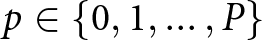 ${p\in\{0, 1, \ldots , P\}}$. Moreover, the LO of the passive radar system is configured to linearly sweep over the whole frequency band of interest, i.e., its starting frequency
  $f_{\textrm{LO0}}$ and stopping frequency
  $f_{\textrm{LO1}}$ are set to
  $f_{\textrm{min}}$ and
  $f_{\textrm{max}}$, respectively. Also, a certain (short) sweep duration denoted as
  $T_{\textrm{LO}}$ is set, such that its frequency course
  $f_{\textrm{LO}}(t)$ is given by
 \begin{equation}
f_{\textrm{LO}}(t) = f_{\textrm{LO0}} + k_{\textrm{LO}} t,
\end{equation}
\begin{equation}
f_{\textrm{LO}}(t) = f_{\textrm{LO0}} + k_{\textrm{LO}} t,
\end{equation} for  $t \in [0, T_{\textrm{LO}}]$, where
 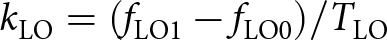 ${k_{\textrm{LO}} = (f_{\textrm{LO1}} - f_{\textrm{LO0}})/ T_{\textrm{LO}}}$ is the ramp slope.
Next we assume that  $f_{\textrm{TX}}(t)$ can be equally expressed as
 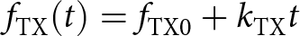 ${f_{\textrm{TX}}(t) = f_{\textrm{TX0}} + k_{\textrm{TX}} t}$ for
  $t \in [0, T_{\textrm{LO}}]$, with an initial frequency
  ${f_{\textrm{TX0}}}$ and a ramp slope
  $k_{\textrm{TX}}$, where
  $|k_{\textrm{TX}}| \lt |k_{\textrm{LO}}|$ holds due to the assumptions. According to (1), this yields for the received frequency courses
 \begin{equation}
f_{\textrm{RX,}p}(t) = f_{\textrm{RX0,}p} + k_{\textrm{RX}} t,
\end{equation}
\begin{equation}
f_{\textrm{RX,}p}(t) = f_{\textrm{RX0,}p} + k_{\textrm{RX}} t,
\end{equation}where
 \begin{equation}
f_{\textrm{RX0,}p} = f_{\textrm{TX0}} - k_{\textrm{TX}} \tau_p ,
\end{equation}
\begin{equation}
f_{\textrm{RX0,}p} = f_{\textrm{TX0}} - k_{\textrm{TX}} \tau_p ,
\end{equation} \begin{equation}
k_{\textrm{RX}} = k_{\textrm{TX}}.
\end{equation}
\begin{equation}
k_{\textrm{RX}} = k_{\textrm{TX}}.
\end{equation} $f_{\textrm{LO}}(t)$ and
  $f_{\textrm{RX,}p}(t)$ will intersect once within the LO chirp duration, i.e.,
 \begin{equation}
f_{\textrm{LO}}(t = t_{\textrm{X,}p}) = f_{\textrm{RX,}p}(t= t_{\textrm{X,}p}),
\end{equation}
\begin{equation}
f_{\textrm{LO}}(t = t_{\textrm{X,}p}) = f_{\textrm{RX,}p}(t= t_{\textrm{X,}p}),
\end{equation} holds for one 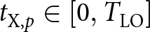 $t_{\textrm{X,}p} \in [0, T_{\textrm{LO}}]$, which is given by
 \begin{equation}
t_{\textrm{X,}p} = \frac{f_{\textrm{LO0}} - f_{\textrm{RX0,}p} }{k_{\textrm{RX}} - k_{\textrm{LO}}}.
\end{equation}
\begin{equation}
t_{\textrm{X,}p} = \frac{f_{\textrm{LO0}} - f_{\textrm{RX0,}p} }{k_{\textrm{RX}} - k_{\textrm{LO}}}.
\end{equation}An example of the previous conditions is shown in fig. 2(a).
An exemplary scenario with interfering FMCW signals captured by a passive radar sensor. (a) Frequency-over-time domain. The LO is configured to perform a (short) sweep over the whole frequency band of interest, allowing to exploit the received signal components stemming from the interferer. Here, 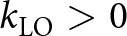 $k_{\textrm{LO}} \gt 0$ and
 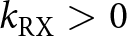 $k_{\textrm{RX}} \gt 0$ was used, yielding
 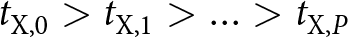 $t_{\textrm{X,}0} \gt t_{\textrm{X,}1} \gt \ldots \gt t_{\textrm{X,}P}$. (b) Spatial-angular domain. Multiple EM waves representing the individual signal components impinge onto the antenna array under different DoAs. Every received signal is downconverted by the same commonly generated LO signal.
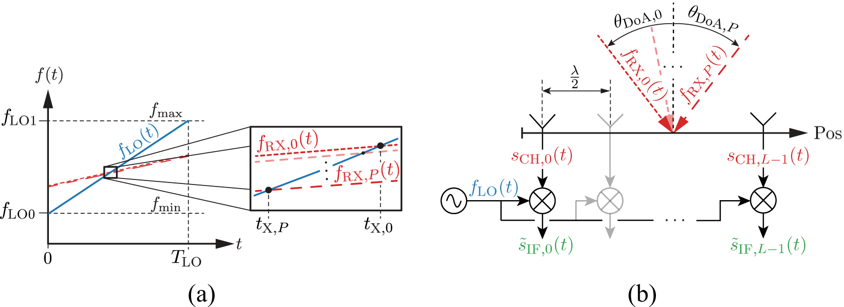
Furthermore, the passive radar sensor is assumed to consist of  $L$ receiving channels of an antenna array, enumerated by
  ${l\in\{0, 1, \ldots , L-1\}}$. In the following, a uniform linear array (ULA) with
  $\lambda/2$ element spacing is considered,
  $\lambda$ being the free space wavelength corresponding to the center frequency of the monitored frequency band. In addition, the EM wave corresponding to the
  $p$th signal path impinges on the antenna array under the angle
  $\theta_{\textrm{DoA,}p}$ with respect to antenna boresight. These conditions are exemplified in fig. 2(b).
Due to the previous considerations, the LO signal for  $t \in [0, T_{\textrm{LO}}]$ can now be expressed as
 \begin{equation}
s_{\textrm{LO}}(t) = A_{\textrm{LO}} {\rm e}^{{\rm j}(2 \pi f_{\textrm{LO0}} t + \pi k_{\textrm{LO}} t^2 + \varphi_{\textrm{LO0}}) } ,
\end{equation}
\begin{equation}
s_{\textrm{LO}}(t) = A_{\textrm{LO}} {\rm e}^{{\rm j}(2 \pi f_{\textrm{LO0}} t + \pi k_{\textrm{LO}} t^2 + \varphi_{\textrm{LO0}}) } ,
\end{equation} with a signal amplitude  $A_{\textrm{LO}}$ and initial phase
  $\varphi_{\textrm{LO0}}$. Furthermore, the received signal at the
  $l$th channel is given by
 \begin{equation}
s_{\textrm{CH,}l}(t) = \sum_{p=0}^{P} A_{\textrm{RX,}p} {\rm e}^{{\rm j}(2\pi f_{\textrm{RX0,}p} t + \pi k_{\textrm{RX}} t^2 + \varphi_{\textrm{RX0,}p} + \pi l u_p) },
\end{equation}
\begin{equation}
s_{\textrm{CH,}l}(t) = \sum_{p=0}^{P} A_{\textrm{RX,}p} {\rm e}^{{\rm j}(2\pi f_{\textrm{RX0,}p} t + \pi k_{\textrm{RX}} t^2 + \varphi_{\textrm{RX0,}p} + \pi l u_p) },
\end{equation} where  $A_{\textrm{RX,}p}$ and
  $\varphi_{\textrm{RX0,}p}$ are signal amplitude and initial phase term of the
  $p$th signal path, respectively, and
  $u_p = \sin\theta_{\textrm{DoA,}p}$. After downconverting each channel with the common LO signal, the resulting
  $l$th IF signal after the mixer (assuming unity gain) can be written as
 \begin{equation}
\begin{aligned}
\tilde{s}_{\textrm{IF,}l}(t) = \sum_{p=0}^{P} \underbrace{A_{\textrm{IF,}p} {\rm e}^{{\rm j}(2 \pi f_{\textrm{IF0,}p} t + \pi k_{\textrm{IF}} t^2 + \varphi_{\textrm{IF0,}p} + \pi l u_p)} }_{ \tilde{s}_{\textrm{IF,}l,p}(t) },
\end{aligned}
\end{equation}
\begin{equation}
\begin{aligned}
\tilde{s}_{\textrm{IF,}l}(t) = \sum_{p=0}^{P} \underbrace{A_{\textrm{IF,}p} {\rm e}^{{\rm j}(2 \pi f_{\textrm{IF0,}p} t + \pi k_{\textrm{IF}} t^2 + \varphi_{\textrm{IF0,}p} + \pi l u_p)} }_{ \tilde{s}_{\textrm{IF,}l,p}(t) },
\end{aligned}
\end{equation}with
 \begin{equation}
A_{\textrm{IF,}p} = A_{\textrm{LO}} A_{\textrm{RX,}p},
\end{equation}
\begin{equation}
A_{\textrm{IF,}p} = A_{\textrm{LO}} A_{\textrm{RX,}p},
\end{equation} \begin{equation}
f_{\textrm{IF0,}p} = f_{\textrm{LO0}} - f_{\textrm{RX0,}p},
\end{equation}
\begin{equation}
f_{\textrm{IF0,}p} = f_{\textrm{LO0}} - f_{\textrm{RX0,}p},
\end{equation} \begin{equation}
k_{\textrm{IF}} = k_{\textrm{LO}} - k_{\textrm{RX}},
\end{equation}
\begin{equation}
k_{\textrm{IF}} = k_{\textrm{LO}} - k_{\textrm{RX}},
\end{equation} \begin{equation}
\varphi_{\textrm{IF0,}p} = \varphi_{\textrm{LO0}} - \varphi_{\textrm{RX0,}p}.
\end{equation}
\begin{equation}
\varphi_{\textrm{IF0,}p} = \varphi_{\textrm{LO0}} - \varphi_{\textrm{RX0,}p}.
\end{equation} $B_{\textrm{IF}}$ and negligible group delay. This yields
 \begin{equation}
s_{\textrm{IF,}l}(t) =
\sum_{p=0}^{P} {\tilde{s}}_{\textrm{IF,}l,p}(t) \mathrm{rect} \left( \frac{k_{\textrm{IF}} t + f_{\textrm{IF0,}p} }{2 B_{\textrm{IF}} } \right) .
\end{equation}
\begin{equation}
s_{\textrm{IF,}l}(t) =
\sum_{p=0}^{P} {\tilde{s}}_{\textrm{IF,}l,p}(t) \mathrm{rect} \left( \frac{k_{\textrm{IF}} t + f_{\textrm{IF0,}p} }{2 B_{\textrm{IF}} } \right) .
\end{equation} Finally, adding a noise term  $w_{\textrm{IF,}l}(t)$ that is assumed to originate from a circular symmetric white Gaussian random process results in
 \begin{equation}
x_{\textrm{IF,}l}(t) = s_{\textrm{IF,}l}(t) + w_{\textrm{IF,}l}(t).
\end{equation}
\begin{equation}
x_{\textrm{IF,}l}(t) = s_{\textrm{IF,}l}(t) + w_{\textrm{IF,}l}(t).
\end{equation} This signal is digitized by the analog-to-digital converter (ADC) at a sampling rate  ${f_\textrm{s}}$, which for automotive radars is usually in the MHz range and is assumed to satisfy
  $f_\textrm{s} \gt 2 B_{\textrm{IF}}$ to prevent aliasing effects. After obtaining
  ${ N= \lfloor T_{\textrm{LO}} f_\textrm{s} \rfloor }$ time domain samples and combining the resulting signals for all
  $L$ channels into a matrix
  ${\mathbf{X}_{\textrm{IF}} \in \mathbb{C}^{N \times L}}$, the resulting signal model using the fast time index
  $n \in \{0, 1, \ldots , N-1\}$ can be expressed as
 \begin{equation}
\mathbf{X}_{\textrm{IF}} = (\mathbf{R}_{\textrm{FT}}(\boldsymbol{\theta}) \odot \mathbf{H}_{\textrm{FT}}(\boldsymbol{\theta})) \mathbf{A}(\boldsymbol{\theta}) \mathbf{H}_{\textrm{AF}}(\boldsymbol{\theta}) + \mathbf{W}(\boldsymbol{\theta}),
\end{equation}
\begin{equation}
\mathbf{X}_{\textrm{IF}} = (\mathbf{R}_{\textrm{FT}}(\boldsymbol{\theta}) \odot \mathbf{H}_{\textrm{FT}}(\boldsymbol{\theta})) \mathbf{A}(\boldsymbol{\theta}) \mathbf{H}_{\textrm{AF}}(\boldsymbol{\theta}) + \mathbf{W}(\boldsymbol{\theta}),
\end{equation}with
 \begin{equation}
[\mathbf{R}_{\textrm{FT}}(\boldsymbol{\theta})]_{n,p} = \mathrm{rect} \left( \frac{k_{\textrm{IF}} n + f_{\textrm{IF0,}p} f_\textrm{s} } {2 B_{\textrm{IF}} f_\textrm{s} } \right),
\end{equation}
\begin{equation}
[\mathbf{R}_{\textrm{FT}}(\boldsymbol{\theta})]_{n,p} = \mathrm{rect} \left( \frac{k_{\textrm{IF}} n + f_{\textrm{IF0,}p} f_\textrm{s} } {2 B_{\textrm{IF}} f_\textrm{s} } \right),
\end{equation} \begin{equation}
[\mathbf{H}_{\textrm{FT}}(\boldsymbol{\theta})]_{n,p} = {\rm e}^{{\rm j}\left(2 \pi \frac{f_{\textrm{IF0,}p}}{f_\textrm{s}} n + \pi \frac{k_{\textrm{IF}}}{f_\textrm{s}^2} n^2 \right)},
\end{equation}
\begin{equation}
[\mathbf{H}_{\textrm{FT}}(\boldsymbol{\theta})]_{n,p} = {\rm e}^{{\rm j}\left(2 \pi \frac{f_{\textrm{IF0,}p}}{f_\textrm{s}} n + \pi \frac{k_{\textrm{IF}}}{f_\textrm{s}^2} n^2 \right)},
\end{equation} \begin{equation}
\mathbf{A}(\boldsymbol{\theta}) = \textrm{diag}([ A_{\textrm{IF,}0} {\rm e}^{{\rm j} \varphi_{\textrm{IF0,}0}}, \ldots , A_{\textrm{IF,}P} {\rm e}^{{\rm j} \varphi_{\textrm{IF0,}P}}]^T),
\end{equation}
\begin{equation}
\mathbf{A}(\boldsymbol{\theta}) = \textrm{diag}([ A_{\textrm{IF,}0} {\rm e}^{{\rm j} \varphi_{\textrm{IF0,}0}}, \ldots , A_{\textrm{IF,}P} {\rm e}^{{\rm j} \varphi_{\textrm{IF0,}P}}]^T),
\end{equation} \begin{equation}
[\mathbf{H}_{\textrm{AF}}(\boldsymbol{\theta})]_{p,l} = {\rm e}^{{\rm j} \pi l u_p},
\end{equation}
\begin{equation}
[\mathbf{H}_{\textrm{AF}}(\boldsymbol{\theta})]_{p,l} = {\rm e}^{{\rm j} \pi l u_p},
\end{equation} \begin{equation}
\textrm{vec}(\mathbf{W}(\boldsymbol{\theta})) \sim \mathcal{CN}(\mathbf{0}, \sigma^2 \mathbf{I}),
\end{equation}
\begin{equation}
\textrm{vec}(\mathbf{W}(\boldsymbol{\theta})) \sim \mathcal{CN}(\mathbf{0}, \sigma^2 \mathbf{I}),
\end{equation} where  $\sigma^2$ is the variance of the complex-valued noise and
 \begin{equation}
\begin{aligned}
\boldsymbol{\theta} =
[&f_{\textrm{IF0,}0}, \ldots , f_{\textrm{IF0,}P}, k_{\textrm{IF}}, A_{\textrm{IF,}0}, \ldots , A_{\textrm{IF,}P}, \\
& \varphi_{\textrm{IF0,}0}, \ldots , \varphi_{\textrm{IF0,}P}, u_0, \ldots , u_P, \sigma^2]^{\rm T},
\end{aligned}
\end{equation}
\begin{equation}
\begin{aligned}
\boldsymbol{\theta} =
[&f_{\textrm{IF0,}0}, \ldots , f_{\textrm{IF0,}P}, k_{\textrm{IF}}, A_{\textrm{IF,}0}, \ldots , A_{\textrm{IF,}P}, \\
& \varphi_{\textrm{IF0,}0}, \ldots , \varphi_{\textrm{IF0,}P}, u_0, \ldots , u_P, \sigma^2]^{\rm T},
\end{aligned}
\end{equation} represents the vector of unknowns, which will be the focus of the signal processing steps in the next section. Notably, due to the lowpass, the amount of time-domain samples is effectively reduced to  $N_{\textrm{IF}} = \textrm{min}(N, \lfloor 2 B_{\textrm{IF}} f_\textrm{s} / |k_{\textrm{IF}}| \rfloor) \le N$ usable samples for the proposed mode of operation, where edge cases are not considered. The lowpass also defines an effective bandwidth
 \begin{equation}
B_{\textrm{eff}} = \min \left( \left| T_{\textrm{LO}} k_{\textrm{RX}} \right|, \left| \frac{2 B_{\textrm{IF}} k_{\textrm{RX}}}{k_{\textrm{LO}} {-} k_{\textrm{RX}}} \right| \right),
\end{equation}
\begin{equation}
B_{\textrm{eff}} = \min \left( \left| T_{\textrm{LO}} k_{\textrm{RX}} \right|, \left| \frac{2 B_{\textrm{IF}} k_{\textrm{RX}}}{k_{\textrm{LO}} {-} k_{\textrm{RX}}} \right| \right),
\end{equation} which will become relevant later when analyzing the accuracy of the object localization. At this point, it is only required that  $N_{\textrm{IF}}$ is sufficiently large such that the subsequent signal processing steps can be performed.
Signal processing
Pre-processing
As already mentioned, many state-of-the-art automotive FMCW radar sensors do not feature an I/Q receiver. Therefore, the spectral components of the real-valued IF signals occur pairwise, one of which is the actual physically relevant component. Consequently, in the following, a pre-processing step that removes the ambiguous signal component is presented, with the intention of ensuring approximate compliance with (11).
The received real-valued IF signals can be modeled by  $\check{\mathbf{X}}_{\textrm{IF}} = \textrm{Re}(\mathbf{X}_{\textrm{IF}})$. First, applying a time-domain Hilbert transform
  $\bar{\mathbf{X}}_{\textrm{IF}} = \mathcal{H}(\check{\mathbf{X}}_{\textrm{IF}})$ removes the negative spectral components. Next, a (coarse) estimate
  $\hat{t}_{\textrm{X}}^{\sim}$ for the intersection points
  $t_{\textrm{X,}p}$ is obtained by computing
 \begin{equation}
\hat{t}_{\textrm{X}}^{\sim} = \frac{1}{L f_\textrm{s}} \sum_{l=0}^{L-1} \frac{\sum_{n=0}^{N-1} n|[\bar{\mathbf{X}}_{\textrm{IF}}]_{n,l}|^2}{\sum_{n=0}^{N-1} |[\bar{\mathbf{X}}_{\textrm{IF}}]_{n,l}|^2},
\end{equation}
\begin{equation}
\hat{t}_{\textrm{X}}^{\sim} = \frac{1}{L f_\textrm{s}} \sum_{l=0}^{L-1} \frac{\sum_{n=0}^{N-1} n|[\bar{\mathbf{X}}_{\textrm{IF}}]_{n,l}|^2}{\sum_{n=0}^{N-1} |[\bar{\mathbf{X}}_{\textrm{IF}}]_{n,l}|^2},
\end{equation}which corresponds to the center of mass of the instantaneous signal powers, averaged over all antenna channels. Finally, a selective phase inversion is performed
 \begin{equation}
[\tilde{\mathbf{X}}_{\textrm{IF}}]_{n,l} = \left\{
\begin{array}{ll}
|[\bar{\mathbf{X}}_{\textrm{IF}}]_{n,l}| {\rm e}^{-{\rm j} \; \textrm{arg}[\bar{\mathbf{X}}_{\textrm{IF}}]_{n,l} } & k_{\textrm{LO}} \gt 0 \;\; n \le \hat{t}_{\textrm{X}}^{\sim} \ f_\textrm{s} , \\
|[\bar{\mathbf{X}}_{\textrm{IF}}]_{n,l}| {\rm e}^{{\rm j} \; \textrm{arg}[\bar{\mathbf{X}}_{\textrm{IF}}]_{n,l} } & k_{\textrm{LO}} \gt 0 \;\; n \gt \hat{t}_{\textrm{X}}^{\sim} \ f_\textrm{s} , \\
|[\bar{\mathbf{X}}_{\textrm{IF}}]_{n,l}| {\rm e}^{{\rm j} \; \textrm{arg}[\bar{\mathbf{X}}_{\textrm{IF}}]_{n,l} } & k_{\textrm{LO}} \lt 0 \;\; n \le \hat{t}_{\textrm{X}}^{\sim} \ f_\textrm{s} , \\
|[\bar{\mathbf{X}}_{\textrm{IF}}]_{n,l}| {\rm e}^{-{\rm j} \; \textrm{arg}[\bar{\mathbf{X}}_{\textrm{IF}}]_{n,l} } & k_{\textrm{LO}} \lt 0 \;\; n \gt \hat{t}_{\textrm{X}}^{\sim} \ f_\textrm{s} , \\
\end{array}
\right.
\end{equation}
\begin{equation}
[\tilde{\mathbf{X}}_{\textrm{IF}}]_{n,l} = \left\{
\begin{array}{ll}
|[\bar{\mathbf{X}}_{\textrm{IF}}]_{n,l}| {\rm e}^{-{\rm j} \; \textrm{arg}[\bar{\mathbf{X}}_{\textrm{IF}}]_{n,l} } & k_{\textrm{LO}} \gt 0 \;\; n \le \hat{t}_{\textrm{X}}^{\sim} \ f_\textrm{s} , \\
|[\bar{\mathbf{X}}_{\textrm{IF}}]_{n,l}| {\rm e}^{{\rm j} \; \textrm{arg}[\bar{\mathbf{X}}_{\textrm{IF}}]_{n,l} } & k_{\textrm{LO}} \gt 0 \;\; n \gt \hat{t}_{\textrm{X}}^{\sim} \ f_\textrm{s} , \\
|[\bar{\mathbf{X}}_{\textrm{IF}}]_{n,l}| {\rm e}^{{\rm j} \; \textrm{arg}[\bar{\mathbf{X}}_{\textrm{IF}}]_{n,l} } & k_{\textrm{LO}} \lt 0 \;\; n \le \hat{t}_{\textrm{X}}^{\sim} \ f_\textrm{s} , \\
|[\bar{\mathbf{X}}_{\textrm{IF}}]_{n,l}| {\rm e}^{-{\rm j} \; \textrm{arg}[\bar{\mathbf{X}}_{\textrm{IF}}]_{n,l} } & k_{\textrm{LO}} \lt 0 \;\; n \gt \hat{t}_{\textrm{X}}^{\sim} \ f_\textrm{s} , \\
\end{array}
\right.
\end{equation} yielding the pre-processed signal  $\tilde{\mathbf{X}}_{\textrm{IF}} \approx \mathbf{X}_{\textrm{IF}}$ that can be used as input to the subsequent processing steps.
Signal component separation
The joint estimation of all unknown parameters in  $\boldsymbol{\theta}$ appears to be impractical due to the high dimensionality of the resulting estimation problem. Therefore, a prior separation of the different signal components based on their different DoAs is proposed. To this end, determination of
  $P$ as well as the corresponding DoAs is initially required. The obtained DoAs allow to synthesize beam steering vectors that maximize the signal energy out of a certain DoA while at the same time suppressing the signal energy from all other DoAs. Also, the obtained DoAs can be used for the localization concept, which will be shown later.
As a first step, the amount of spatial frequencies corresponding to  $P$ has to be detected. For this task, state-of-the-art model order selection criteria such as power-spectrum-based constant false alarm rate (CFAR) detection, minimum description length (MDL) or Akaike information criterion (AIC) can be used [Reference Djukanovic and Popovic-Bugarin21, Reference Javidi da Costa, Thakre, Roemer and Haardt22]. Next, a (scaled) estimate of the array correlation matrix
  $\mathbf{R}_{\mathbf{ll}}$ is obtained by using all available time-domain samples as snapshots
  ${\hat{\mathbf{R}}_{\mathbf{ll}} = \mathbf{X}_{\textrm{IF}}^H \mathbf{X}_{\textrm{IF}}}$. Subsequently, standard beamforming techniques like delay-and-sum, Capon, or multiple signal classification (MUSIC) can be applied to this matrix, depending on the required angular resolution in relation to the given array size.
Assuming that  $P$ has been correctly identified, the beamforming step yields
  $P+1$ estimates for the DoAs
  ${\hat{\theta}_{\textrm{DoA,}0}, \ldots , \hat{\theta}_{\textrm{DoA,}P}}$ which can be used to generate
  $P+1$ beam steering vectors. Ideally, the
  $p$th beam steering vector
  $\mathbf{b}_{p}$ should be chosen such that
  ${[\mathbf{H}_{\textrm{AF}} \mathbf{b}_{p}^{*}]_{p'} = c_p \delta_{pp'}}$ holds for a certain
  $c_p \ne 0$,
  $\delta$ being the Kronecker delta and
  ${p' \in\{0, 1, \ldots , P\}}$. In this work, we propose to apply the null-steering-based least squares error pattern synthesis method for this purpose [Reference Van Trees23]. Afterwards, the individual signal components
  $\mathbf{x}_{\textrm{IF,}p}$ can be obtained by
  ${\mathbf{x}_{\textrm{IF,}p} = \mathbf{X}_{\textrm{IF}} \mathbf{b}_{p}^{*}}$. According to (11),
  $\mathbf{x}_{\textrm{IF,}p}$ can be modeled as
 \begin{equation}
\mathbf{x}_{\textrm{IF,}p} = (\mathbf{f}_{\textrm{FT},p}(\boldsymbol{\theta}_p) \odot \mathbf{h}_{\textrm{FT},p}(\boldsymbol{\theta}_p) ) a_p(\boldsymbol{\theta}_p) + \mathbf{w}_p(\boldsymbol{\theta}_p),
\end{equation}
\begin{equation}
\mathbf{x}_{\textrm{IF,}p} = (\mathbf{f}_{\textrm{FT},p}(\boldsymbol{\theta}_p) \odot \mathbf{h}_{\textrm{FT},p}(\boldsymbol{\theta}_p) ) a_p(\boldsymbol{\theta}_p) + \mathbf{w}_p(\boldsymbol{\theta}_p),
\end{equation}with
 \begin{equation}
[\mathbf{f}_{\textrm{FT},p}]_{n} = \mathrm{rect} \left( \frac{k_{\textrm{IF}} n + f_{\textrm{IF0,}p} f_\textrm{s} } {2 B_{\textrm{IF}} f_\textrm{s} } \right),
\end{equation}
\begin{equation}
[\mathbf{f}_{\textrm{FT},p}]_{n} = \mathrm{rect} \left( \frac{k_{\textrm{IF}} n + f_{\textrm{IF0,}p} f_\textrm{s} } {2 B_{\textrm{IF}} f_\textrm{s} } \right),
\end{equation} \begin{equation}
[\mathbf{h}_{\textrm{FT},p}]_{n} = {\rm e}^{{\rm j}\left(2 \pi \frac{f_{\textrm{IF0,}p}}{f_\textrm{s}} n + \pi \frac{k_{\textrm{IF}}}{f_\textrm{s}^2} n^2 \right)},
\end{equation}
\begin{equation}
[\mathbf{h}_{\textrm{FT},p}]_{n} = {\rm e}^{{\rm j}\left(2 \pi \frac{f_{\textrm{IF0,}p}}{f_\textrm{s}} n + \pi \frac{k_{\textrm{IF}}}{f_\textrm{s}^2} n^2 \right)},
\end{equation} \begin{equation}
a_p = c_p A_{\textrm{IF,}p} {\rm e}^{{\rm j} \varphi_{\textrm{IF0,}p}},
\end{equation}
\begin{equation}
a_p = c_p A_{\textrm{IF,}p} {\rm e}^{{\rm j} \varphi_{\textrm{IF0,}p}},
\end{equation} \begin{equation}
\mathbf{w}_p \sim \mathcal{CN}(\mathbf{0}, \sigma_p^2 \mathbf{I}),
\end{equation}
\begin{equation}
\mathbf{w}_p \sim \mathcal{CN}(\mathbf{0}, \sigma_p^2 \mathbf{I}),
\end{equation}and a reduced vector of unknowns
 \begin{equation}
\boldsymbol{\theta}_p = [\,f_{\textrm{IF0,}p}, k_{\textrm{IF}}, A_{\textrm{IF,}p}, \varphi_{\textrm{IF0,}p}, \sigma_p^2]^{\rm T}.
\end{equation}
\begin{equation}
\boldsymbol{\theta}_p = [\,f_{\textrm{IF0,}p}, k_{\textrm{IF}}, A_{\textrm{IF,}p}, \varphi_{\textrm{IF0,}p}, \sigma_p^2]^{\rm T}.
\end{equation}Time-frequency estimation
In this section, we will investigate the optimal estimation of  $\boldsymbol{\theta}_p$ with the goal of obtaining a time-frequency sample of the interfering waveform with the best possible precision. To this end, the estimation of
  $\boldsymbol{\theta}_p$ in an ML sense is proposed as a first step. Considering (15), the ML estimator is found by maximizing
 \begin{equation}
\hat{\boldsymbol{\theta}}_p' = \mathop{\arg\max}_{\boldsymbol{\theta}_p'} {\underbrace{| (\mathbf{f}_{\textrm{FT},p} \odot \mathbf{h}_{\textrm{FT},p})^H \mathbf{x}_{\textrm{IF,}p} |^2 }_{J'(\boldsymbol{\theta}_p')}},
\end{equation}
\begin{equation}
\hat{\boldsymbol{\theta}}_p' = \mathop{\arg\max}_{\boldsymbol{\theta}_p'} {\underbrace{| (\mathbf{f}_{\textrm{FT},p} \odot \mathbf{h}_{\textrm{FT},p})^H \mathbf{x}_{\textrm{IF,}p} |^2 }_{J'(\boldsymbol{\theta}_p')}},
\end{equation} where  ${\boldsymbol{\theta}_p' = [f_{\textrm{IF0,}p}, k_{\textrm{IF}}]^T}$ is a reduced (concentrated) parameter vector and
  $J'(\boldsymbol{\theta}_p')$ is the (concentrated) likelihood function. In order to further elaborate the estimation concept, examples for
  $J'(\boldsymbol{\theta}_p')$ were simulated using the parameters summarized in Table 1 for
  $p=0$ and a noiseless scenario. The results are shown in fig. 3(a), where two different IF bandwidths are compared. As evident, in the case of the lower IF bandwidth, the energy within the likelihood function is spread over a larger area, indicating that the estimation of
  $\boldsymbol{\theta}_p'$ becomes more imprecise in a noisy scenario.
Exemplary concentrated likelihood functions for both a high and a low  $B_\textrm{IF}$. (a) Original parameter space. Due to the energy spread, estimation of
  $f_{\textrm{IF0,}0}$ becomes more imprecise at a lower IF bandwidth. (b) Transformed parameter space. The energy spread is minimized in the direction of
  $f_{\textrm{RXX,}0}$, allowing its precise estimation also in case of a low IF bandwidth.

Parameter set for simulation of likelihood functions

For the aspect of spectral sensing,  $f_{\textrm{IF0,}p}$ could theoretically be used to obtain the time-frequency sample
  $(t{=}0, f{=}f_{\textrm{RX0,}p})$ according to (3). However, since cost-efficient automotive FMCW radar sensors typically feature IF bandwidths in the order of the lower simulated bandwidth, the estimation accuracy would be unsatisfactory. Therefore, we propose applying a coordinate transformation to a different frequency that can be estimated with high precision also in the case of low IF bandwidths. To this end, note that
  $t_{\textrm{X,}p}$ defined in (5) can, according to (8b) and (8c), also be expressed through
  $\boldsymbol{\theta}_p'$ as
 \begin{equation}
t_{\textrm{X,}p}(\boldsymbol{\theta}_p') = \frac{f_{\textrm{IF0,p}}}{k_{\textrm{IF}}}.
\end{equation}
\begin{equation}
t_{\textrm{X,}p}(\boldsymbol{\theta}_p') = \frac{f_{\textrm{IF0,p}}}{k_{\textrm{IF}}}.
\end{equation} Furthermore, considering the corresponding instantaneous frequency  $f_{\textrm{RXX,}p} = f_{\textrm{RX,}p}(t= t_{\textrm{X,}p})$ given by (3) results in
 \begin{equation}
f_{\textrm{RXX,}p}(\boldsymbol{\theta}_p') = f_{\textrm{LO0}} + \frac{k_{\textrm{LO}}}{k_{\textrm{IF}}} f_{\textrm{IF0,p}}.
\end{equation}
\begin{equation}
f_{\textrm{RXX,}p}(\boldsymbol{\theta}_p') = f_{\textrm{LO0}} + \frac{k_{\textrm{LO}}}{k_{\textrm{IF}}} f_{\textrm{IF0,p}}.
\end{equation} This relationship allows to express the concentrated likelihood functions in terms of the transformed parameter vector  ${\boldsymbol{\theta}_p^{\prime\prime} = [f_{\textrm{RXX,}p}, k_{\textrm{IF}}]^T}$, which is shown in fig. 3(b). As evident, the spread of energy is now maximized along
  $k_{\textrm{IF}}$ and minimized along the
  $f_{\textrm{RXX,}p}$-direction, indicating that the coupling between both variables is minimized. This observation suggests that
  $f_{\textrm{RXX,}p}$ can be estimated more precisely than
  $f_{\textrm{IF0,}p}$, which is further supported by the performance comparison shown in Figure 4. Accordingly, at an exemplary SNR of
  $10\,\mathrm{dB}$,
  $f_{\textrm{RXX,}p}$ yields a moderate root mean squared error (RMSE) of
  $\approx 60\,\mathrm{kHz}$, whereas for
  $f_{\textrm{IF0,}p}$ it is
  $\approx 20\,\mathrm{MHz}$.
Comparison of RMSE of  $\hat{f}_{\textrm{IF0,}0}$ and
  $\hat{f}_{\textrm{RXX,}0}$ for a high and a low IF bandwidth, obtained by Monte-Carlo simulations. The transformation of the frequency variable yields a significant performance improvement.

The proposed time-frequency point that can be used for passive spectral sensing is therefore given by  $(t{=}t_{\textrm{X,}p}, f{=}f_{\textrm{RXX,}p})$. Although the estimates can be very similar for different path indices
  $p$, their precise determination will become important for the aspect of object localization, which will be explained in the next section.
Object localization
As mentioned previously, joint DoA-TDoA-based object localization is proposed. To this end, the direct and the indirect signal path created by an object will be conceptually assigned to the reference and surveillance channel within the passive radar framework, respectively. This can be achieved by first identifying the direct signal path, e.g., by choosing the signal component with the highest  $A_{\textrm{IF,p}}$. Next, the TDoA information for the (indirect) signal paths
  $p \gt 0$ with respect to the direct signal path, denoted as
  $\tau_{p0}$, can be computed. Its general definition
  ${\tau_{p0} = \tau_{p} - \tau_{0}}$ can be re-expressed using the results from (3b), (3a), (8b), (8c) and (18) as
 \begin{equation}
\tau_{p0} = \frac{k_{\textrm{IF}}}{k_{\textrm{LO}}} \frac{f_{\textrm{RXX,}p} - f_{\textrm{RXX,}0}}{k_{\textrm{LO}} - k_{\textrm{IF}}},
\end{equation}
\begin{equation}
\tau_{p0} = \frac{k_{\textrm{IF}}}{k_{\textrm{LO}}} \frac{f_{\textrm{RXX,}p} - f_{\textrm{RXX,}0}}{k_{\textrm{LO}} - k_{\textrm{IF}}},
\end{equation} which contains the results from the previous time-frequency estimation step as well as the known value for  $k_{\textrm{LO}}$. The corresponding geometric representation of
  $\tau_{p0}$ is given by an (iso-TDoA) ellipse
  $E_{p}$ with both the passive and the interfering radar sensor located at its foci. Therefore, in order to use
  $\tau_{p0}$ for localization, the position of the interferer
  $P_0$ with respect to the passive radar sensor has to be determined. In the following, a triangulation-based solution using a second (auxiliary) radar sensor in addition to the first (primary) radar sensor is proposed for this purpose. Ideally, this auxiliary radar sensor is placed such that dilution of precision (DOP) for triangulation is minimized, while at the same time, a stable direct signal path to the interferer can be maintained. One suitable way could be to place both radar sensors close to the outer bumper corners of the passively sensing vehicle. In addition, the auxiliary radar sensor applies the same sweeping LO and signal processing steps as the primary sensor, and its LO ramps can be triggered using a coarse time synchronization link to the primary radar sensor. Even though this sensor could be used to further improve the overall localization quality in a passive radar network setup, in this work, it will only be used for the purpose of finding
  $P_0$. Therefore, after identifying the primary signal path at both primary and auxiliary radar stations, the corresponding values
  $\theta_{\textrm{DoA,}0}$ and
  $\theta_{\textrm{DoA,}0}'$ yield lines
  $L_{0}$ and
  $L_{0}'$ as geometric representations, and their intersection point yields
  $P_0$ in a suitable coordinate system. Considering that
  $P_0$ and
  $\tau_{p0}$ now fully define
  $E_{p}$, and that
  $L_{p}$ further denotes the geometric line representation corresponding to
  $\theta_{\textrm{DoA,}p}$ of an object, the latter can be localized by computing the geometric intersection point between
  $E_{p}$ and
  $L_{p}$, denoted as
  $P_p$. This localization procedure is summarized and depicted in fig. 5.
Visualization of the proposed localization principle using a primary and an auxiliary radar sensor. Firstly, the position of the interferer  $P_0$ is determined by triangulation of
  $L_{0}$ and
  $L_{0}'$. Secondly, the position of another object in the scene
  $P_p$ is given by intersecting
  $L_{p}$ and
  $E_{p}$.

For completeness, it should be noted that the interferer could also be localized by evaluating TDoA information between the primary and the auxiliary radar sensor [Reference Liu, Yang and Wang24]. However, since such a method requires a fine time synchronization (in the order of a few ns) between the primary and auxiliary radar sensor, it may not be practical for every automotive radar setup.
Multiple LO ramps
The focus of the preceding sections was on interference exploitation using an individual LO ramp. However, in automotive radar sensors, usually multiple consecutive LO ramps are performed (chirp sequence). Considering that an interferer is usually present for a period longer than that of a single LO ramp, in many cases, multiple of the received IF signals will be affected. This can be ensured due to the sweeping of the LO over the whole automotive frequency band, in particular for interferers with changing starting frequencies in a stepped FMCW modulation scheme and/or time and frequency dithering. While  $\boldsymbol{\theta}$ in (11f) and the resulting time-frequency point generally being different for each IF signal, the positions of the interferer and surrounding objects may still be considered as similar for many IF signals. Therefore, averaging of these positions (
 $P_0$ and
  $P_p$) is proposed to improve the quality of the localization. As will be shown in the next analysis section, this strategy will benefit in particular interference scenarios with a low effective bandwidth
  $B_{\textrm{eff}}$ and only a few interfered samples
  $N_{\textrm{IF}}$, where the localization accuracy using only a single ramp would be insufficient. The latter case will also be shown in the measurement section, where the averaging significantly reduces the variances of the resulting localization estimates.
Theoretical analysis
SNR range
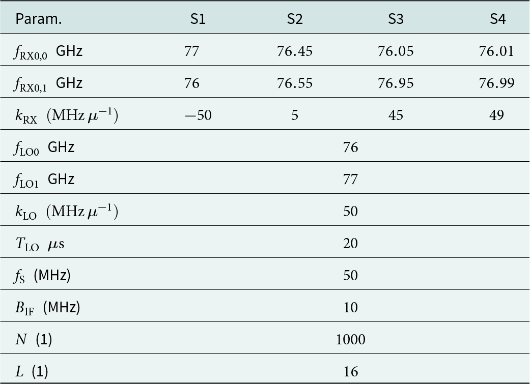
In order to assess the practicability of the proposed concept, evaluating the possible range of SNRs created by an interfering signal is of special interest. To this end, the primary radar station is assumed to be located at the origin of a 2-D Cartesian coordinate system. In addition, the interferer and an object are assumed to be located at  $\boldsymbol{P}_0 =[x_{\textrm{0}},y_{\textrm{0}}]$ and
  $\boldsymbol{P}_1 = [x_{\textrm{1}},y_{\textrm{1}}]$, respectively.
The SNR for the direct signal path based on the radar equation is given by
 \begin{equation}
\textrm{SNR}_0 = \frac{P_{\textrm{TX}} G_{\textrm{TX}} G_{\textrm{RX}} \lambda^2}{\left(4\pi c_0 \tau_0 \right)^2 k_\textrm{B} T_\textrm{S} B_{\textrm{IF}} F},
\end{equation}
\begin{equation}
\textrm{SNR}_0 = \frac{P_{\textrm{TX}} G_{\textrm{TX}} G_{\textrm{RX}} \lambda^2}{\left(4\pi c_0 \tau_0 \right)^2 k_\textrm{B} T_\textrm{S} B_{\textrm{IF}} F},
\end{equation}and further for the indirect signal path assuming a reflection at a flat widespread object with proper alignment
 \begin{equation}
\textrm{SNR}_1 = \frac{
P_{\textrm{TX}} G_{\textrm{TX}} G_{\textrm{RX}} \lambda^2 } {(4\pi c_0 \tau_1)^2 k_\textrm{B} T_\textrm{S} B_{\textrm{IF}} F},
\end{equation}
\begin{equation}
\textrm{SNR}_1 = \frac{
P_{\textrm{TX}} G_{\textrm{TX}} G_{\textrm{RX}} \lambda^2 } {(4\pi c_0 \tau_1)^2 k_\textrm{B} T_\textrm{S} B_{\textrm{IF}} F},
\end{equation} where  $P_{\textrm{TX}}$ is the transmit power of the interferer,
  $G_{\textrm{TX}}$ and
  $G_{\textrm{RX}}$ are the antenna gains of the interferer and the primary station, respectively. Furthermore,
  $\lambda$ is the wavelength,
  $k_\textrm{B}$ is the Boltzmann constant, and
  $T_\textrm{S}$ and
  $F$ are the primary stations’ system temperature and noise figure, respectively. Also, the corresponding path delays are given by
 \begin{equation}
\tau_0 = \frac{1}{c_0} \sqrt{x_{\textrm{0}}^2 + y_{\textrm{0}}^2},
\end{equation}
\begin{equation}
\tau_0 = \frac{1}{c_0} \sqrt{x_{\textrm{0}}^2 + y_{\textrm{0}}^2},
\end{equation} \begin{equation}
\tau_1 = \frac{1}{c_0} \left( \sqrt{x_{\textrm{1}}^2 + y_{\textrm{1}}^2} + \sqrt{(x_{\textrm{0}}-x_{\textrm{1}})^2 + (y_{\textrm{0}}-y_{\textrm{1}})^2} \right),
\end{equation}
\begin{equation}
\tau_1 = \frac{1}{c_0} \left( \sqrt{x_{\textrm{1}}^2 + y_{\textrm{1}}^2} + \sqrt{(x_{\textrm{0}}-x_{\textrm{1}})^2 + (y_{\textrm{0}}-y_{\textrm{1}})^2} \right),
\end{equation} where  $c_0$ is the speed of light.
In order to also cover the influence of the antenna beampattern, we assume patch antenna elements with a cosine-squared amplitude dependency (field of view (FOV)  $\approx 65^{\circ}$) on the DoA for both the interferer and the primary station. If alignment of the antenna boresight directions with the y-axis is assumed, this yields
 \begin{equation}
G_{\textrm{TX}} = G_{\textrm{TX,max}} \left( \frac{|y_{\textrm{1}}|}{\sqrt{x_{\textrm{1}}^2 + y_{\textrm{1}}^2}} \right)^4,
\end{equation}
\begin{equation}
G_{\textrm{TX}} = G_{\textrm{TX,max}} \left( \frac{|y_{\textrm{1}}|}{\sqrt{x_{\textrm{1}}^2 + y_{\textrm{1}}^2}} \right)^4,
\end{equation} \begin{equation}
G_{\textrm{RX}} = G_{\textrm{RX,max}} \left(\frac{|y_{\textrm{1}}|}{\sqrt{x_{\textrm{1}}^2 + y_{\textrm{1}}^2}} \right)^4,
\end{equation}
\begin{equation}
G_{\textrm{RX}} = G_{\textrm{RX,max}} \left(\frac{|y_{\textrm{1}}|}{\sqrt{x_{\textrm{1}}^2 + y_{\textrm{1}}^2}} \right)^4,
\end{equation} where  $G_{\textrm{TX,max}}$ and
  $G_{\textrm{RX,max}}$ are the antenna gains of the interferer and the primary station in boresight direction, respectively. In the sequel, the following values were chosen to model a typical automotive setup:
 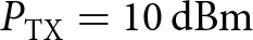 $P_{\textrm{TX}} = 10\,\mathrm{dBm}$,
  $G_{\textrm{TX,max}} = G_{\textrm{RX,max}} = 10\mathrm{dBi}$,
 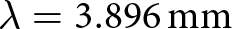 $\lambda = 3.896\,\mathrm{mm}$,
 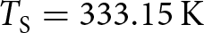 $T_\textrm{S} = 333.15\,\mathrm{K}$,
 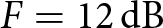 $F = 12\,\mathrm{dB}$.
Figure 6(a) shows the resulting Iso-SNR contour plot of the direct signal path as a function of the interferer position  $\boldsymbol{P}_0$. Furthermore, fig. 6(a) shows an Iso-SNR contour plot of the indirect signal path as a function of the position of an object
  $\boldsymbol{P}_1$, where a fixed interferer position
 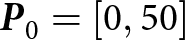 $\boldsymbol{P}_0 = [0, 50]$ has been used. These results show that
  $\textrm{SNR}_0$ can be over
  $30\mathrm{dB}$ for interferers closer than
  $10\,\mathrm{m}$ and close to boresight direction (e.g., a front and a rear radar of two vehicles driving one behind the other in a dense urban traffic environment). Also, larger distances such as
  $50\,\mathrm m$ can still yield considerable
  $17\,\mathrm{dB}$ of SNR. However, if the two radar sensors leave their mutual FOV (e.g., two front radars of two vehicles driving past each other), the influence of the antenna beampattern quickly reduces the available SNR. Similarly,
  $\textrm{SNR}_1$, which is limited by
  $\textrm{SNR}_0$ at the corresponding interferer position (
 $17\,\mathrm{dB}$ in this example), also degrades significantly for objects outside the mutual FOV.
Iso-SNR contour plots. (a) Direct signal path ( $\textrm{SNR}_0$) for different interferer positions
  $\boldsymbol{P}_0$. (b) Indirect signal path (
 $\textrm{SNR}_1$) for different object positions
  $\boldsymbol{P}_1$ and fixed interferer position
  $\boldsymbol{P}_0 = [0, 50]$.

The SNR determines not only whether the interference can be reliably detected, but also the localization accuracy of objects. Both points will be analyzed in the next sections.
Minimum SNR
An important aspect with respect to the SNR is the minimum SNR for the algorithm to be applicable. Generally speaking, this minimum SNR is defined by requirements in terms of signal detectability in the first place. A limiting factor for the proposed signal detection in the angular domain is given by the estimate of  $\hat{t}_{\textrm{X}}^{\sim}$ in (13). Its estimation quality can be assessed by means of RMSE curves, which were simulated for four different interference scenarios S1–S4 summarized in Table 2. While S1 and S2 create short (
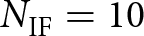 $N_{\textrm{IF}} = 10$ and
 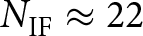 $N_{\textrm{IF}} \approx 22$) and S3 medium-extended (
 $N_{\textrm{IF}} = 200$) interference patterns in the time-domain signal, for S4 all
  $N_{\textrm{IF}} = 1000$ samples of the IF signal are interfered. The resulting curves are shown in fig. 7. In accordance with the expectations, the RMSE decreases with increasing SNR, where the decrease starts at lower SNRs for larger
  $N_{\textrm{IF}}$. For an RMSE below 1 sample, the algorithm requires an SNR in the range
 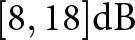 $[8, 18] \mathrm{dB}$, depending on the scenario. According to the previous SNR analysis, these values are realistic for a large range of possible interferer positions, such that a reasonable performance can be generally assumed. Noteworthy, since this analysis is not completely exhaustive, the provided SNR range represents a coarse estimate only. Additional requirements for the SNR can be further imposed by requirements on localization accuracy, which will be discussed next.
RMSE simulation for minimum SNR assessment.

Parameter set for SNR and localization accuracy analysis
Localization accuracy
In this section, the accuracy of the proposed DoA-TDoA-based localization method will be investigated by means of DOP analysis for scenarios S1-S4. As will be seen, the localization accuracy depends on the position of both the interferer 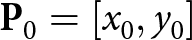 $\mathbf{P}_0 = [x_0,y_0]$ and the object
  $\mathbf{P}_p = [x_p,y_p]$ to be localized relative to the passive radar stations. This is due to not only the properties of the geometric localization approach, but also the SNR of the interference present at the receiver.
For this analysis, the SNR is again modeled according to (20) and (21). In order to fully specify the parameter vector  $\boldsymbol{\theta}$ in (11f) we further set the arbitrary phase arguments to
 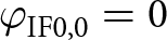 $\varphi_\textrm{IF0,0}=0$ and
  $\varphi_\textrm{IF0,1}=0$, and the noise variance to
 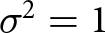 $\sigma^2=1$ since for the accuracy of the proposed localization method only the SNR is relevant. For simplicity, it is further assumed that
  $\boldsymbol{\theta}$ is jointly estimated in an ML sense. Its error covariance matrix
  $\boldsymbol{C}_{\boldsymbol{\theta}\boldsymbol{\theta}}$ is for large data records is consequently given by
 \begin{equation} \boldsymbol{C}_{\boldsymbol{\theta}\boldsymbol{\theta}} =\boldsymbol{I}^{-1}_{\boldsymbol{\theta}}(\boldsymbol{\theta}) ,
\end{equation}
\begin{equation} \boldsymbol{C}_{\boldsymbol{\theta}\boldsymbol{\theta}} =\boldsymbol{I}^{-1}_{\boldsymbol{\theta}}(\boldsymbol{\theta}) ,
\end{equation} with the Fisher information matrix  $\boldsymbol{I}_{\boldsymbol{\theta}}(\boldsymbol{\theta}) $ defined by
 \begin{equation}
[\boldsymbol{I}_{\boldsymbol{\theta}}(\boldsymbol{\theta})]_{a,b} = - \mathbb{E} \left[ \frac{\partial^2 \log p(\mathbf{X}_{\textrm{IF}}; \boldsymbol{\theta}) }
{\partial \theta_{a} \partial \theta_{b} } \right], \end{equation}
\begin{equation}
[\boldsymbol{I}_{\boldsymbol{\theta}}(\boldsymbol{\theta})]_{a,b} = - \mathbb{E} \left[ \frac{\partial^2 \log p(\mathbf{X}_{\textrm{IF}}; \boldsymbol{\theta}) }
{\partial \theta_{a} \partial \theta_{b} } \right], \end{equation} where  $p(\mathbf{X}_{\textrm{IF}}; \boldsymbol{\theta})$ is the probability density function (PDF) of
  $\mathbf{X}_{\textrm{IF}}$ parameterized by
  $\boldsymbol{\theta}$, and
  $a, b\in \{0, \ldots 4P+5\}$. Its convenient computation for the problem at hand (
 $P=1$) is possible by applying the result from [Reference Kay25, p. 525] to the transformed parameter vector
 \begin{equation}
\begin{aligned}
\boldsymbol{\theta}_{\textrm{loc}} =
[&f_{\textrm{IF0,}0}, f_{\textrm{IF0,}1}, k_{\textrm{IF}}, a_{\textrm{IF,}0}, a_{\textrm{IF,}1}, \\
& b_{\textrm{IF,}0}, b_{\textrm{IF,}P}, u_0, u_1, \sigma^2]^{\rm T},
\end{aligned}
\end{equation}
\begin{equation}
\begin{aligned}
\boldsymbol{\theta}_{\textrm{loc}} =
[&f_{\textrm{IF0,}0}, f_{\textrm{IF0,}1}, k_{\textrm{IF}}, a_{\textrm{IF,}0}, a_{\textrm{IF,}1}, \\
& b_{\textrm{IF,}0}, b_{\textrm{IF,}P}, u_0, u_1, \sigma^2]^{\rm T},
\end{aligned}
\end{equation}where
 \begin{equation}
a_{\textrm{IF,}0} = A_{\textrm{IF,}0} \cos \varphi_{\textrm{IF0,}0},
\end{equation}
\begin{equation}
a_{\textrm{IF,}0} = A_{\textrm{IF,}0} \cos \varphi_{\textrm{IF0,}0},
\end{equation} \begin{equation}
a_{\textrm{IF,}1} = A_{\textrm{IF,}1} \cos \varphi_{\textrm{IF0,}1},
\end{equation}
\begin{equation}
a_{\textrm{IF,}1} = A_{\textrm{IF,}1} \cos \varphi_{\textrm{IF0,}1},
\end{equation} \begin{equation}
b_{\textrm{IF,}0} = A_{\textrm{IF,}0} \sin \varphi_{\textrm{IF0,}0},
\end{equation}
\begin{equation}
b_{\textrm{IF,}0} = A_{\textrm{IF,}0} \sin \varphi_{\textrm{IF0,}0},
\end{equation} \begin{equation}
b_{\textrm{IF,}0} = A_{\textrm{IF,}1} \sin\varphi_{\textrm{IF0,}1}.
\end{equation}
\begin{equation}
b_{\textrm{IF,}0} = A_{\textrm{IF,}1} \sin\varphi_{\textrm{IF0,}1}.
\end{equation}This yields the Fisher information matrix
 \begin{equation}
\mathbf{I}_{\boldsymbol{\theta}_{\textrm{loc}}} = \begin{bmatrix}
\frac{2}{\sigma^2} \textrm{Re}(\boldsymbol{D}^\textrm{H} \boldsymbol{D}) & \boldsymbol{0} \\
\boldsymbol{0}^\textrm{T} & \frac{NL}{(\sigma^2)^2} \\
\end{bmatrix},
\end{equation}
\begin{equation}
\mathbf{I}_{\boldsymbol{\theta}_{\textrm{loc}}} = \begin{bmatrix}
\frac{2}{\sigma^2} \textrm{Re}(\boldsymbol{D}^\textrm{H} \boldsymbol{D}) & \boldsymbol{0} \\
\boldsymbol{0}^\textrm{T} & \frac{NL}{(\sigma^2)^2} \\
\end{bmatrix},
\end{equation} \begin{equation}
\boldsymbol{D} = [\boldsymbol{D}_{f}, \boldsymbol{d}_{k}, \boldsymbol{D}_{A}, {\rm j}\boldsymbol{D}_{A}, \boldsymbol{D}_{u}],
\end{equation}
\begin{equation}
\boldsymbol{D} = [\boldsymbol{D}_{f}, \boldsymbol{d}_{k}, \boldsymbol{D}_{A}, {\rm j}\boldsymbol{D}_{A}, \boldsymbol{D}_{u}],
\end{equation} \begin{equation}
\boldsymbol{D}_{f} = \mathbf{H}_{\textrm{AF}}^{\rm T} \ast (\mathbf{R}_{\textrm{FT}} \odot \mathbf{D}_{N} \mathbf{H}_{\textrm{FT}} ) \mathbf{A},
\end{equation}
\begin{equation}
\boldsymbol{D}_{f} = \mathbf{H}_{\textrm{AF}}^{\rm T} \ast (\mathbf{R}_{\textrm{FT}} \odot \mathbf{D}_{N} \mathbf{H}_{\textrm{FT}} ) \mathbf{A},
\end{equation} \begin{equation}
\boldsymbol{d}_{k} = \mathbf{H}_{\textrm{AF}}^{\rm T} \ast (\mathbf{R}_{\textrm{FT}} \odot \mathbf{D}_{N^2} \mathbf{H}_{\textrm{FT}} ) \mathbf{A} \mathbf{1},
\end{equation}
\begin{equation}
\boldsymbol{d}_{k} = \mathbf{H}_{\textrm{AF}}^{\rm T} \ast (\mathbf{R}_{\textrm{FT}} \odot \mathbf{D}_{N^2} \mathbf{H}_{\textrm{FT}} ) \mathbf{A} \mathbf{1},
\end{equation} \begin{equation}
\boldsymbol{D}_{A} = \mathbf{H}_{\textrm{AF}}^{\rm T} \ast (\mathbf{R}_{\textrm{FT}} \odot \mathbf{H}_{\textrm{FT}} ) ,
\end{equation}
\begin{equation}
\boldsymbol{D}_{A} = \mathbf{H}_{\textrm{AF}}^{\rm T} \ast (\mathbf{R}_{\textrm{FT}} \odot \mathbf{H}_{\textrm{FT}} ) ,
\end{equation} \begin{equation}
\boldsymbol{D}_{u} = \mathbf{D}_{L} \mathbf{H}_{\textrm{AF}}^{\rm T} \ast (\mathbf{R}_{\textrm{FT}} \odot \mathbf{H}_{\textrm{FT}} ) \mathbf{A},
\end{equation}
\begin{equation}
\boldsymbol{D}_{u} = \mathbf{D}_{L} \mathbf{H}_{\textrm{AF}}^{\rm T} \ast (\mathbf{R}_{\textrm{FT}} \odot \mathbf{H}_{\textrm{FT}} ) \mathbf{A},
\end{equation} \begin{equation}
\boldsymbol{D}_{N} = \textrm{diag}({\rm j} 2 \pi [0, \ldots , N-1]^\textrm{T}),
\end{equation}
\begin{equation}
\boldsymbol{D}_{N} = \textrm{diag}({\rm j} 2 \pi [0, \ldots , N-1]^\textrm{T}),
\end{equation} \begin{equation}
\boldsymbol{D}_{N^2} = \textrm{diag}({\rm j} \pi ([0, \ldots , N-1]^\textrm{T} \odot [0, \ldots , N-1]^\textrm{T})),
\end{equation}
\begin{equation}
\boldsymbol{D}_{N^2} = \textrm{diag}({\rm j} \pi ([0, \ldots , N-1]^\textrm{T} \odot [0, \ldots , N-1]^\textrm{T})),
\end{equation} \begin{equation}
\boldsymbol{D}_{L} = \textrm{diag}({\rm j} \pi [0, \ldots , L-1]^\textrm{T}),
\end{equation}
\begin{equation}
\boldsymbol{D}_{L} = \textrm{diag}({\rm j} \pi [0, \ldots , L-1]^\textrm{T}),
\end{equation} $\ast$ denotes the Khatri–Rao or block Kronecker product, and
  $\boldsymbol{1}$ and
  $\boldsymbol{0}$ are vectors containing all ones and zeros, respectively. Noteworthy, for this computation it has been assumed that
  $\mathbf{R}_{\textrm{FT}}$ does not depend on
  $f_{\textrm{IF0,}0}, f_{\textrm{IF0,}1}$ and
  $ k_{\textrm{IF}}$ for simplicity. Also, the notational dependency on
  $\boldsymbol{\theta}_{\textrm{loc}}$ was omitted for better readability.
Next, the error covariance matrix for the parameter vector  $\boldsymbol{\theta_{1,\textrm{loc}}} = [u_{\textrm{1}}, \tau_{10}]^T$, which is required for DoA-TDoA-based object localization is given by the relation [Reference Kay25]
 \begin{equation}
\boldsymbol{C}_{\boldsymbol{\theta_{1,\textrm{loc}}} \boldsymbol{\theta_{1,\textrm{loc}}}} = \frac{\partial \boldsymbol{\theta_{\textrm{1,loc}}}}{\partial \boldsymbol{\theta_{\textrm{loc}}}} \boldsymbol{I}^{-1}_{\boldsymbol{\theta_{\textrm{loc}}}} \frac{\partial \boldsymbol{\theta_{\textrm{1,loc}}}^T}{\partial \boldsymbol{\theta_{\textrm{loc}}}},
\end{equation}
\begin{equation}
\boldsymbol{C}_{\boldsymbol{\theta_{1,\textrm{loc}}} \boldsymbol{\theta_{1,\textrm{loc}}}} = \frac{\partial \boldsymbol{\theta_{\textrm{1,loc}}}}{\partial \boldsymbol{\theta_{\textrm{loc}}}} \boldsymbol{I}^{-1}_{\boldsymbol{\theta_{\textrm{loc}}}} \frac{\partial \boldsymbol{\theta_{\textrm{1,loc}}}^T}{\partial \boldsymbol{\theta_{\textrm{loc}}}},
\end{equation}where
 \begin{equation}
\left[ \frac{\partial \boldsymbol{\theta_{\textrm{1,loc}}}}{\partial \boldsymbol{\theta_{\textrm{loc}}}} \right]_{c,a} = \left\{
\begin{array}{ll}
1 & c=0, a=8\\
-\frac{1}{k_{\textrm{LO}} - k_{\textrm{IF}}} & c=1, a=0\\[5pt]
\frac{1}{k_{\textrm{LO}} - k_{\textrm{IF}}} & c=1, a=1\\[5pt]
\frac{f_{\textrm{IF0,0}} - f_{\textrm{IF0,1}}}{(k_{\textrm{LO}} - k_{\textrm{IF}})^2} & c=1, a=2\\[5pt]
0 & \, \textrm{else}, \\
\end{array}
\right.
\end{equation}
\begin{equation}
\left[ \frac{\partial \boldsymbol{\theta_{\textrm{1,loc}}}}{\partial \boldsymbol{\theta_{\textrm{loc}}}} \right]_{c,a} = \left\{
\begin{array}{ll}
1 & c=0, a=8\\
-\frac{1}{k_{\textrm{LO}} - k_{\textrm{IF}}} & c=1, a=0\\[5pt]
\frac{1}{k_{\textrm{LO}} - k_{\textrm{IF}}} & c=1, a=1\\[5pt]
\frac{f_{\textrm{IF0,0}} - f_{\textrm{IF0,1}}}{(k_{\textrm{LO}} - k_{\textrm{IF}})^2} & c=1, a=2\\[5pt]
0 & \, \textrm{else}, \\
\end{array}
\right.
\end{equation} and  $c \in \{0, 1\}$.
Finally, the relation of  $\boldsymbol{\theta_{\textrm{1,loc}}}$ to
  $\mathbf{P}_1 = [x_1, y_1]$ is given by the sensor measurement residual equations
  $\boldsymbol{f} = [f_1(\boldsymbol{\theta_{\textrm{1,loc}}}, \mathbf{P}_1), f_2(\boldsymbol{\theta_{\textrm{1,loc}}}, \mathbf{P}_1)]^{\rm T}$
 \begin{equation}
f_1(\boldsymbol{\theta_{\textrm{1,loc}}}, \mathbf{P}_1) = u_{\textrm{1}} +\frac{x_{\textrm{1}}}{\sqrt{x_{\textrm{1}}^2+y_{\textrm{1}}^2}}= 0,
\end{equation}
\begin{equation}
f_1(\boldsymbol{\theta_{\textrm{1,loc}}}, \mathbf{P}_1) = u_{\textrm{1}} +\frac{x_{\textrm{1}}}{\sqrt{x_{\textrm{1}}^2+y_{\textrm{1}}^2}}= 0,
\end{equation} \begin{equation}
\begin{aligned}
& f_2(\boldsymbol{\theta_{\textrm{1,loc}}}, \mathbf{P}_1) = \tau_{\textrm{10}} - \frac{1}{c_0}\left( \sqrt{x_{\textrm{1}}^2+y_{\textrm{1}}^2} + \right. \\
& \left. \sqrt{(x_{\textrm{1}}-x_{\textrm{0}})^2+(y_{\textrm{1}}-y_{\textrm{0}})^2} - \sqrt{x_{\textrm{0}}^2+y_{\textrm{0}}^2} \right) = 0.
\end{aligned}
\end{equation}
\begin{equation}
\begin{aligned}
& f_2(\boldsymbol{\theta_{\textrm{1,loc}}}, \mathbf{P}_1) = \tau_{\textrm{10}} - \frac{1}{c_0}\left( \sqrt{x_{\textrm{1}}^2+y_{\textrm{1}}^2} + \right. \\
& \left. \sqrt{(x_{\textrm{1}}-x_{\textrm{0}})^2+(y_{\textrm{1}}-y_{\textrm{0}})^2} - \sqrt{x_{\textrm{0}}^2+y_{\textrm{0}}^2} \right) = 0.
\end{aligned}
\end{equation} DOP analysis, which assumes that (33) is solved by applying the best linear unbiased estimator (BLUE) to a linearized version of the equation system [Reference Langley26], yields the error covariance matrix  $\boldsymbol{C}_{\mathbf{P}_1\mathbf{P}_1}$ given by
 \begin{equation}
\boldsymbol{C}_{\mathbf{P}_1\mathbf{P}_1} = ( \mathbf{J}_{\mathbf{P}_1}^{{\rm T}} (\mathbf{J}_{\boldsymbol{\theta_{1,\textrm{loc}}}} \boldsymbol{I}^{-1}_{\boldsymbol{\theta_{1,\textrm{loc}}}}(\boldsymbol{\theta}) \mathbf{J}_{\boldsymbol{\theta_{1,\textrm{loc}}}}^{{\rm T}} )^{-1} \mathbf{J}_{\mathbf{P}_1})^{-1},
\end{equation}
\begin{equation}
\boldsymbol{C}_{\mathbf{P}_1\mathbf{P}_1} = ( \mathbf{J}_{\mathbf{P}_1}^{{\rm T}} (\mathbf{J}_{\boldsymbol{\theta_{1,\textrm{loc}}}} \boldsymbol{I}^{-1}_{\boldsymbol{\theta_{1,\textrm{loc}}}}(\boldsymbol{\theta}) \mathbf{J}_{\boldsymbol{\theta_{1,\textrm{loc}}}}^{{\rm T}} )^{-1} \mathbf{J}_{\mathbf{P}_1})^{-1},
\end{equation} \begin{equation}
\mathbf{J}_{\boldsymbol{\theta_{1,\textrm{loc}}}} = \frac{\partial \boldsymbol{f}}{\partial \boldsymbol{\theta_{1,\textrm{loc}}}} ,
\end{equation}
\begin{equation}
\mathbf{J}_{\boldsymbol{\theta_{1,\textrm{loc}}}} = \frac{\partial \boldsymbol{f}}{\partial \boldsymbol{\theta_{1,\textrm{loc}}}} ,
\end{equation} \begin{equation}
\mathbf{J}_{\mathbf{P}_1} = \frac{\partial \boldsymbol{f}}{\partial \mathbf{P}_1} ,
\end{equation}
\begin{equation}
\mathbf{J}_{\mathbf{P}_1} = \frac{\partial \boldsymbol{f}}{\partial \mathbf{P}_1} ,
\end{equation} \begin{equation}
\mathbf{J}_{\boldsymbol{\theta_{1,\textrm{loc}}}} = \begin{bmatrix}
1 & 0 \\
0 & 1 \\
\end{bmatrix},
\end{equation}
\begin{equation}
\mathbf{J}_{\boldsymbol{\theta_{1,\textrm{loc}}}} = \begin{bmatrix}
1 & 0 \\
0 & 1 \\
\end{bmatrix},
\end{equation} \begin{equation}
[ \mathbf{J}_{\boldsymbol{x}_{\textrm{1}}}]_{0,0} = \frac{y_{\textrm{1}}^2}{(x_{\textrm{1}}^2 + y_{\textrm{1}}^2)^{3/2}},
\end{equation}
\begin{equation}
[ \mathbf{J}_{\boldsymbol{x}_{\textrm{1}}}]_{0,0} = \frac{y_{\textrm{1}}^2}{(x_{\textrm{1}}^2 + y_{\textrm{1}}^2)^{3/2}},
\end{equation} \begin{equation}
[ \mathbf{J}_{\boldsymbol{x}_{\textrm{1}}}]_{0,1} = \frac{- x_{\textrm{1}} y_{\textrm{1}} }{(x_{\textrm{1}}^2 + y_{\textrm{1}}^2)^{3/2}} ,
\end{equation}
\begin{equation}
[ \mathbf{J}_{\boldsymbol{x}_{\textrm{1}}}]_{0,1} = \frac{- x_{\textrm{1}} y_{\textrm{1}} }{(x_{\textrm{1}}^2 + y_{\textrm{1}}^2)^{3/2}} ,
\end{equation} \begin{equation}
\begin{aligned}
{[{{\boldsymbol{J}}_{{{\boldsymbol{x}}_{\rm{1}}}}}]_{1,0}} = - \frac{1}{{{c_0}}}\left( {\frac{{{x_{\rm{1}}}}}{{\sqrt {x_{\rm{1}}^2 + y_{\rm{1}}^2} }}} \right.\\
\left. { - \frac{{{x_{\rm{0}}} - {x_{\rm{1}}}}}{{\sqrt {{{\left( {{x_{\rm{0}}} - {x_{\rm{1}}}} \right)}^2} + {{\left( {{y_{\rm{0}}} - {y_{\rm{1}}}} \right)}^2}} }}} \right),
\end{aligned}
\end{equation}
\begin{equation}
\begin{aligned}
{[{{\boldsymbol{J}}_{{{\boldsymbol{x}}_{\rm{1}}}}}]_{1,0}} = - \frac{1}{{{c_0}}}\left( {\frac{{{x_{\rm{1}}}}}{{\sqrt {x_{\rm{1}}^2 + y_{\rm{1}}^2} }}} \right.\\
\left. { - \frac{{{x_{\rm{0}}} - {x_{\rm{1}}}}}{{\sqrt {{{\left( {{x_{\rm{0}}} - {x_{\rm{1}}}} \right)}^2} + {{\left( {{y_{\rm{0}}} - {y_{\rm{1}}}} \right)}^2}} }}} \right),
\end{aligned}
\end{equation} \begin{equation}
\begin{aligned}
{[{{\boldsymbol{J}}_{{{\boldsymbol{x}}_{\rm{1}}}}}]_{1,1}} = \frac{1}{{{c_0}}}\left( {\frac{{{y_{\rm{1}}}}}{{\sqrt {y_{\rm{1}}^2 + x_{\rm{1}}^2} }}} \right.\\
\left. { - \frac{{{y_{\rm{0}}} - {y_{\rm{1}}}}}{{\sqrt {{{\left( {{y_{\rm{0}}} - {y_{\rm{1}}}} \right)}^2} + {{\left( {{x_{\rm{0}}} - {x_{\rm{1}}}} \right)}^2}} }}} \right).
\end{aligned}
\end{equation}
\begin{equation}
\begin{aligned}
{[{{\boldsymbol{J}}_{{{\boldsymbol{x}}_{\rm{1}}}}}]_{1,1}} = \frac{1}{{{c_0}}}\left( {\frac{{{y_{\rm{1}}}}}{{\sqrt {y_{\rm{1}}^2 + x_{\rm{1}}^2} }}} \right.\\
\left. { - \frac{{{y_{\rm{0}}} - {y_{\rm{1}}}}}{{\sqrt {{{\left( {{y_{\rm{0}}} - {y_{\rm{1}}}} \right)}^2} + {{\left( {{x_{\rm{0}}} - {x_{\rm{1}}}} \right)}^2}} }}} \right).
\end{aligned}
\end{equation} In fig. 8,  $\boldsymbol{C}_{\mathbf{P}_1\mathbf{P}_1}$ is visualized by means of error ellipses for different positions of
  $\mathbf{P}_1$ and a fixed interferer position
  $\mathbf{P}_0 = [0, 50]$ for all defined scenarios. Noteworthy, for S3 and S4 the error ellipses are no longer visible due to their small size. Therefore, in fig. 9, a zoomed-in version of the error ellipse for
  $\mathbf{P}_1 = [-10,25]$ is additionally provided.
Visualization of  $\boldsymbol{C}_{\mathbf{P}_1\mathbf{P}_1}$ (error ellipses) for different positions of
  $\mathbf{P}_1$ and a fixed interferer position
  $\mathbf{P}_0 = [0, 50]$ for all defined scenarios. Noteworthy, for S3 and S4 the error ellipses are no longer visible due to their small extent.

Zoomed-in visualization of  $\boldsymbol{C}_{\mathbf{P}_1\mathbf{P}_1}$ (error ellipses) of
  $\mathbf{P}_1 = [-10, 25]$ and a fixed interferer position
  $\mathbf{P}_0 = [0, 50]$ for all defined scenarios.

Several aspects are worth mentioning at this point. First, by analyzing the error ellipses for a fixed scenario, it can be seen that their extent and orientation depend on the actual position of the object  $\mathbf{P}_1$. As known from other TDoA-based localization approaches, the forward scattering region close to the baseline between Txb and Rxb1 generally yields poorer localization accuracies. This can be seen, e.g., by comparing the extent of the error ellipses for
  $\mathbf{P}_1 = [-10,25]$ and
  ${\mathbf P}_1=\lbrack-5,25\rbrack$, where the latter is closer to the baseline. The same degradation holds for objects too far outside the FOVs of both radar sensors, e.g.,
  ${\mathbf P}_1=\lbrack10,1\rbrack$, due to a low
  $\textrm{SNR}_1$. It can be concluded that localization using interfering radar signals works best for objects with a certain baseline distance while still being in the FOVs, e.g.,
  $\mathbf{P}_1 = [-10,25]$ or
  $\mathbf{P}_1 = [10,40]$ in this example.
Second, from the orientation of the error ellipses, it can be assessed which of the two quantities - DoA or TDoA - limits the overall localization accuracy. An alignment of the major axis to  $L_1$ or
  $E_1$’s tangential vector indicates limitation by TDoA or DoA, respectively. To this end, note that the orientation of the error ellipse in fig. 9 changes between the scenarios. For S1 and S2, the amount of interfered fast-time samples required for TDoA estimation is low, whereas in S3 and S4, it is significantly higher. On the other hand, the amount of spatial samples required for DoA estimation is the same for all scenarios. Therefore, TDoA-based localization accuracy can benefit from a significant temporal processing gain, making the method particularly useful for interferers with relatively high ramp slopes.
Third, by comparing the sizes of the error ellipses for different scenarios, it can be seen that the resulting localization accuracy strongly depends on the interferer ramp slope  $k_{\textrm{RX}}$ in combination with the resulting temporal processing gain. The importance of the ramp slope becomes evident by comparing S1 with S2, where S1 yields a higher accuracy than S2 despite a lower
  $N_\textrm{IF}$. In fact,
  $k_{\textrm{RX}}$ is encoded in the effective bandwidth
  $B_{\textrm{eff}}$, which determines the TDoA estimation accuracy. The best result with accuracies in the centimeters range can therefore be achieved for high values of both
  $B_{\textrm{eff}}$ and
  $N_{\textrm{IF}}$ such as in S3 or S4. As previously mentioned, insufficient accuracies such as in S1 and S2 can be accommodated by averaging the estimates over multiple LO ramps.
It should be emphasized that this analysis has been based on a range of (simplifying and/or optimistic) assumptions that are not strictly fulfilled for the proposed algorithmic localization method. Nevertheless, these results can still be used as a general indication of the performance to be expected in different interference scenarios, which can serve as a basis for further investigations or optimizations. For completeness, it is also noted that, while this analysis focused exclusively on the object localization, it can also be performed for interferer localization by incorporating a signal model for the auxiliary radar sensor. While beyond the scope of this work, at this point we only point out that the SNR limitation imposed by the antenna beampattern naturally also holds for this case. Therefore, its localization and consequently also the localization of other objects work best if the interfering radar is within the FOV of both passive radar sensors.
Computational complexity analysis
In this section, the computational complexity of the proposed algorithmic concept is analyzed in terms of operations (additions, multiplications, and others). To this end, the following assumptions were made:
• Complex-valued multiplications correspond to four real-valued multiplications and two real-valued additions.
• Complex-valued additions correspond to two real-valued additions.
• The Hilbert transform is performed by zeroing in the frequency domain, for which a radix-2 FFT implementation is used.
• For beamforming, a conventional delay-and-sum approach with a zero-padding factor of
 $Z_L$ is used.
• The CFAR detector is implemented by comparing the power spectrum, which is output by the delay-and-sum beamformer, to a constant threshold.
• For the generation of the beam steering vectors using the proposed null-steering-based least squares error pattern synthesis method, the inverse of the constraint matrix is computed using a conventional Gauss-Jordan approach.
• The ML estimation is implemented by means of a grid search over
$\boldsymbol{\theta}_p^{\prime\prime}$. To this end,
$N_f$ grid points for
$f_{\textrm{RXX,}p}$ and
$N_k$ grid points for
$k_{\textrm{IF}}$ are assumed.• Identifying the direct path using
$A_{\textrm{IF,}p}$ is equivalently achieved by searching for the index
$p'$ which maximizes
$J^{\prime\prime}(\hat{\boldsymbol{\theta}}_p')$.• For DoA-TDoA-based localization, a closed-form expression for the geometric intersection point is evaluated.
• The analysis is performed for the primary radar sensor, which also serves as an upper bound for the auxiliary radar sensor.


The resulting amounts of operations are summarized in Table 3. For an exemplary system with the parameters 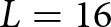 $L=16$,
 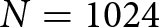 $N=1024$,
  $P=1$,
 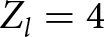 $Z_l = 4$,
 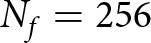 $N_f = 256$,
  $N_k = 16$ this results in a total of
  $\approx 3 \cdot 10^{6}$ operations. At an exemplary automotive microcontroller unit (MCU) with a system clock of
  $400\,\mathrm{MHz}$ and
  $2$ operations per clock cycle this results in an execution time of
  $\approx 151\,\mathrm{ms}$. If parallelization and pre-computation of values are also taken into account, e.g., for the evaluation of the likelihood function, assuming
  $16$ processing cores of equal functionality, the execution time can be further reduced to
 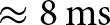 $\approx 8\,\mathrm{ms}$. For a whole sequence of LO ramps and sequential execution, this value is scaled accordingly. Therefore, usual update cycle times of
  $50\,\mathrm{ms}$ are only possible for the proposed passive interference exploitation mode using a small amount of ramps. However, with future improvements of the algorithm and/or the available hardware, real-time processing of even a higher number of ramps could become feasible.
Amount of operations for each processing step
Measurements
In order to demonstrate the feasibility of the presented concept under controlled conditions, measurements were performed in an anechoic chamber. The corresponding setup is shown in fig. 10, which should model an automotive traffic scenario. It consists of three identical radar boards, denoted as  $\textrm{Txb}$,
  $\textrm{Rxb1}$ and
  $\textrm{Rxb2}$, as well as a movable metal plate, denoted as
  $\textrm{P}$. In this setup,
  $\textrm{Txb}$ represents the radar sensor of an interfering vehicle, whereas
  $\textrm{Rxb1}$ and
  $\textrm{Rxb2}$ represent the primary and auxiliary radar stations of the passively sensing vehicle, respectively. Furthermore, the metal plate which has been properly aligned should model a nearby road user or obstacle at the same height as the other radar sensors. Due to the geometric constraint of the anechoic chamber, the distance between
  $\textrm{Txb}$ and
  $\textrm{Rxb1}$ was chosen as approximately
  $4\,\mathrm{m}$, whereas the baseline distance between
  $\textrm{Rxb1}$ and
  $\textrm{Rxb2}$ was in the area of
  $1\mathrm{m}$.
Measurement setup in anechoic chamber.  $\textrm{Txb}$ represents the radar sensor of an interfering vehicle, whereas
  $\textrm{Rxb1}$ and
  $\textrm{Rxb2}$ represent the primary and auxiliary radar sensors of the passively sensing vehicle, respectively. Both radar sensors receive a direct signal by the interferer. Furthermore, a metal plate
  $\textrm{P}$ is added to the setup, which creates an additional indirect signal path captured by
  $\textrm{Rxb1}$.

All radar stations used in the setup are 77-GHz FMCW radar boards from INRAS featuring 2 TX and 16 RX channels each. At  $\textrm{Txb}$, one TX is actively transmitting, whereas at
  $\textrm{Rxb1}$ and
  $\textrm{Rxb2}$ signals are recorded at all 16 RX channels which constitute a ULA. The communication with the boards is performed via Ethernet, and the data is stored and processed at an external laptop.
For the measurement, the chosen key system parameters are shown in Table 4, which already represents a challenging interference scenarios with a low effective bandwidth  $B_{\textrm{eff}} \approx 1.16\,\mathrm{MHz}$ and only few interfered samples
  $N_{\textrm{IF}} \approx 29$. Notably, the parameters
  ${f_{\textrm{TX0}} }$,
  ${f_{\textrm{TX1}} }$ and
  ${T_{\textrm{TX}} }$ corresponding to
  $\textrm{Txb}$ are defined in analogy to
  ${f_{\textrm{LO0}} }$,
  ${f_{\textrm{LO1}} }$ and
  ${T_{\textrm{LO}}}$, respectively. Furthermore,
  $\textrm{Txb}$ periodically repeats its frequency ramp after the repetition time
  ${T_{\textrm{TX,rep}} }$, whereas
  $\textrm{Rxb1}$ and
  $\textrm{Rxb2}$ perform
  $M$ consecutive LO ramps with a repetition time of
  ${T_{\textrm{LO,rep}}}$ between the ramps.
Parameter set for measurement
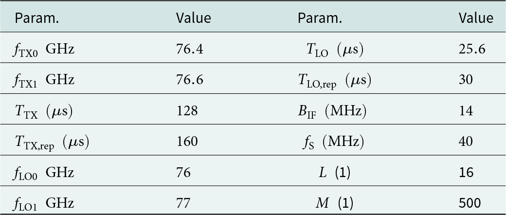
The output of the time-frequency estimation stage is shown in fig. 11(a) for the first 6 LO ramps of  $\textrm{Rxb1}$ and
  $p=0$. It can be seen that the estimated time-frequency points match the actual crossing points between each LO upramp of
  $f_{\textrm{LO}}(t)$ and
  $f_{\textrm{RX,}0}(t)$ well. These points may further be used, e.g., to determine the ramp parameters of the interferer and/or to avoid the spectrally congested region for further active radar operations.
Measurement results. (a) Frequency courses  $f_{\textrm{LO}}(t)$,
  $f_{\textrm{RX,}0}(t)$ as well as the estimated time-frequency points
  $(\hat{t}_{\textrm{X,}0} / \hat{f}_{\textrm{RXX,}0})$ which match the actual crossing points well. (b) Estimated probability distributions displayed in yellow and green for the positions of
  $\textrm{Txb}$ and
  $P$, respectively. Furthermore, the distribution means
  $\widehat{\textrm{Txb}}$,
  $\hat{P}$, and their
  $1\sigma$ confidence bounds are shown for two different positions of
  $P$. In both scenarios, the resulting positional estimates match the ground truths up to a few centimeters.

Moreover, the output of the object localization stage is shown in fig. 11(b) for two different positions of the metal plate. It displays an estimated probability density of the positional estimates for  $\textrm{Txb}$ and
  $P$ as well as their distribution means
  $\widehat{\textrm{Txb}}$ and
  $\hat{\text{P}}$, using all
  $M=500$ LO ramps. It can be seen that the distribution means match the actual ground truths
  $\textrm{Txb}$ and
  $P$ up to a few centimeters for both positions of the metal plate. Noteworthy, since the proposed estimation concept directly solves the nonlinear equation system (33) by means of geometric intersection rather than solving its linearized version, the resulting probability densities can appear skewed compared to an ellipse. This is in particular the case for this measurement scenario, where the nonlinearity becomes emphasized by the relatively large TDoA variance as a result of a relatively low
  $B_{\textrm{eff}}$. Nevertheless, this experiment shows that multiple ramps can be used to significantly improve the localization accuracy also for otherwise challenging interference scenarios. As mentioned in the introduction, the determined positions could now be further processed, e.g., to support ADAS functionalities.
Conclusion
In this work, we presented and successfully demonstrated a method that for the first time allows to realize both passive spectral sensing and object localization using automotive FMCW signals in an interference exploitation context. The usage of a sweeping LO for this purpose has the advantage that no synchronization onto the interfering waveform is required, which makes the method particularly useful for interferers that change their ramp parameters over time. We theoretically analyzed the applicability of the method by discussing SNR ranges, minimum required SNR, object localization accuracy for different interference scenarios, and computational complexity. Furthermore, the provided measurement results in a challenging interference scenario confirm the effectiveness of both time-frequency estimation and object localization capabilities with an accuracy of a few centimeters.
Acknowledgements
The authors wish to acknowledge the Christian Doppler Research Association as well as Infineon Technologies Austria AG for the funding of this work conducted at the Christian Doppler Laboratory for Distributed Microwave and Terahertz Systems for Sensors and Data Links.
Competing interests
The authors declare none.

Lukas Rienessl was born in Linz, Austria, in 1997. He received the B.Sc. and the Dipl.-Ing. (M.Sc.) degrees in electronics and information technology from Johannes Kepler University, Linz, Austria, in 2020 and 2022, respectively. In 2022, he joined the Institute for Communications Engineering and RF-Systems, where he is currently working toward the Ph.D. degree in collaboration with Infineon Technologies Austria. In 2024, he became a Member of the Christian Doppler Laboratory for Distributed Microwave and Terahertz Systems for Sensors and Data Links. His research interests include radar signal processing concepts and techniques with a focus on passive sensing for automotive radar applications.

Michael Gerstmair was born in Linz, Austria, in 1986. He obtained his Bachelor’s degree in Telematics from Graz University of Technology, Austria, in 2013, and his Dipl.-Ing. degree in Information Electronics from Johannes Kepler University, Linz, Austria, in 2016. From 2016 to 2020, he pursued his Ph.D. degree at Infineon Technologies Linz in collaboration with the Institute of Signal Processing at JKU, Austria, and was awarded his Ph.D. in 2022. His research concentrated on RF impairments in highly integrated radar front ends and radar signal processing for automotive applications. Since 2020, he has been working as a Concept Engineer at Infineon Technologies Linz. He is the primary author of various journal and conference papers and holds several patents in the field of automotive radar systems. Mr. Gerstmair has received the Infineon Austria Innovation Award and the Upper Austrian State Award for Road Safety in 2020 and 2021, respectively.

Christian M. Schmid was born in Vienna, Austria, in 1983. He received the Dipl.-Ing. (M.Sc.) and the Ph.D. degrees in mechatronics from Johannes Kepler University (JKU), Linz, Austria. During his time as an M.Sc. student, he was a visiting student at Prof. Tatsuo Itoh’s Microwave Electronics Laboratory, University of California, Los Angeles, in 2008. In 2009, he joined the Christian Doppler Laboratory for Integrated Radar Sensors, JKU, Linz. In 2014, he joined Infineon Technologies. As a Senior Principal Product Architect, he currently works on 77-GHz ICs for automotive applications. His research interests include RF system design and signal processing for MIMO radar systems. Mr. Schmid served as IEEE Region 8 Student Representative and IEEE Region 8 Secretary. He was the recipient of a German VDI award in 2009 and of the 2012 European Conference on Antennas and Propagation (EuCAP) Best Measurement Paper Prize.

Andreas Stelzer received the Diploma Engineer degree in electrical engineering from the Technical University of Vienna, Austria, in 1994, and the Dr. techn. (Ph.D.) degree in mechatronics from Johannes Kepler University (JKU) Linz, Austria, in 2000. In 2003, he became an Associate Professor at Johannes Kepler University Linz. Since 2011, he has been a Full Professor heading the Department for RF-Systems. His research focuses on microwave sensor systems for industrial and automotive applications, integrated sensor concepts, SiGe-based circuit design, RF and microwave subsystems, as well as signal processing for sensor signal evaluation. Dr. Stelzer has authored or coauthored more than 430 papers and received several awards including the European Microwave Association (EuMA) Radar Prize in 2003, the 2008 IEEE Microwave Theory and Techniques Society (IEEE MTT-S) Outstanding Young Engineer Award, the 2011 German Microwave Conference (GeMiC) Best Paper Award, the 2011 IEEE Microwave Prize, and the Best Paper Award of the International Journal of Microwave and Wireless Technologies (IJMWT) 2016. He was an IEEE Distinguished Microwave Lecturer from 2014 to 2016 and Chair of the IEEE International Conference on Microwaves for Intelligent Mobility (ICMIM) in 2020.

Reinhard Feger was born in Kufstein, Austria, in 1980. He received the Dipl.-Ing. (M.Sc.) degree in mechatronics and the Dr. Techn. (Ph.D.) degree in mechatronics from Johannes Kepler University Linz, Austria, in 2005 and 2010, respectively. In 2005, he joined the Institute for Communications and Information Engineering, Johannes Kepler University Linz, where he is currently an Associate Professor and Head of the Christian Doppler Laboratory for Distributed Microwave and Terahertz Systems for Sensors and Data Links. His research topics are radar signal processing, as well as radar system design for industrial and automotive radar sensors.
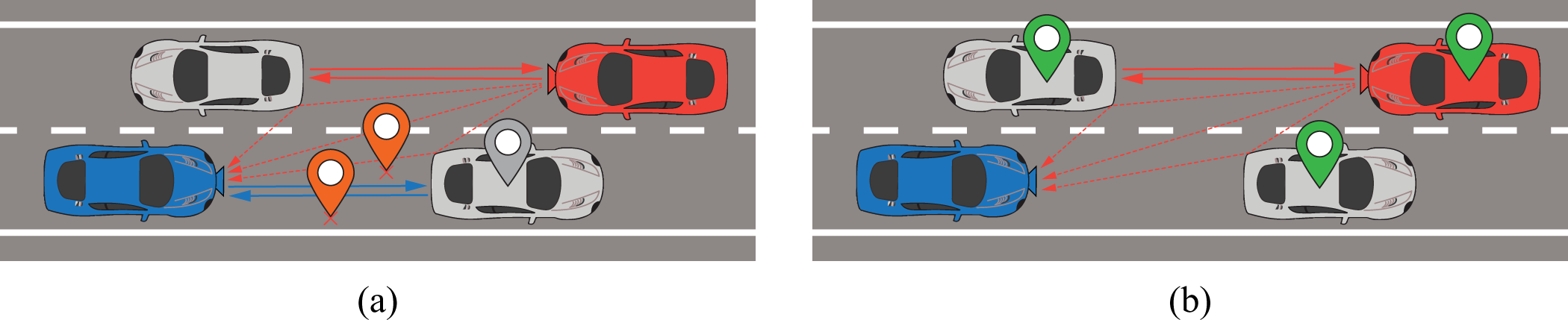


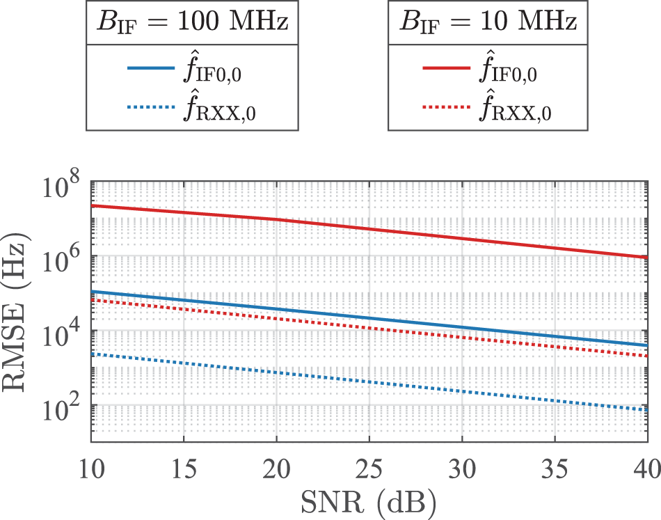


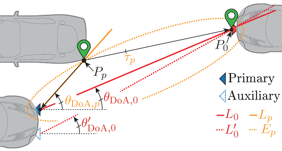


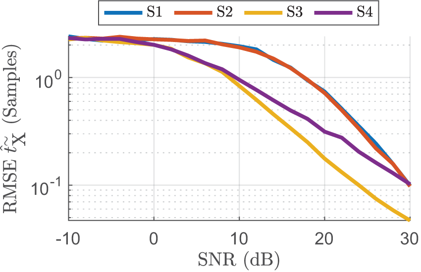
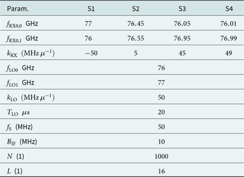


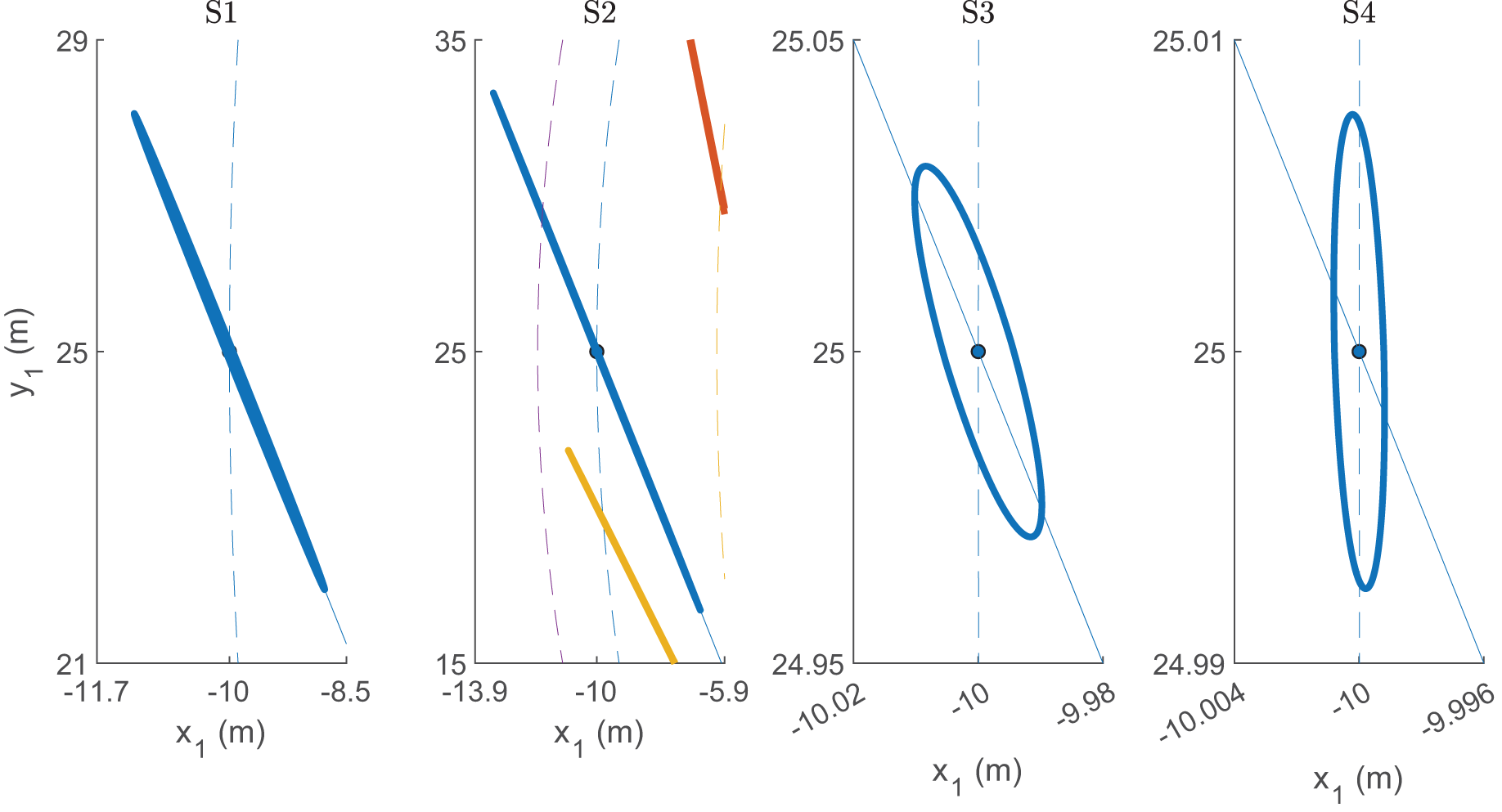


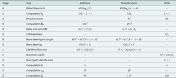


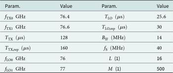


 Open access