





1. Introduction
Our discussion begins with the Kähler Calabi–Yau threefold. Our broad goal is to understand the geometric properties of these complex manifolds as they undergo deformation. Various mechanisms for the degeneration and resolution of Calabi–Yau structures exist, and in this work we focus on the conifold transition.
A conifold transition is a process where a birational contraction of holomorphic curves is followed by a deformation of complex structure. We denote a conifold transition by
 \[\widehat{X} \rightarrow X_0 \rightsquigarrow X_t. \]
In this process, holomorphic curves in $\widehat{X}$
are mapped to singular points in the analytic space
$\widehat{X}$
are mapped to singular points in the analytic space $X_0$
, and the singularities are locally modeled by
$X_0$
, and the singularities are locally modeled by $0 \in \{ \sum z_i^2 = 0 \} \subset \mathbb{C}^4$
. The smoothings
$0 \in \{ \sum z_i^2 = 0 \} \subset \mathbb{C}^4$
. The smoothings $X_t$
deform the complex structure of
$X_t$
deform the complex structure of $X_0$
in a way which is locally modeled by
$X_0$
in a way which is locally modeled by $\{ \sum z_i^2 = t\} \subset \mathbb{C}^4$
.
$\{ \sum z_i^2 = t\} \subset \mathbb{C}^4$
.
As the initial threefold $\hat{X}$
is deformed into
$\hat{X}$
is deformed into $X_t$
, its Hodge numbers undergo jumps. This implies that distinct threefolds with varying topologies can be interconnected through this deformation process. It is conjectured that all Kähler Calabi–Yau threefolds can be linked by conifold transitions [Reference Candelas, Green and HübschCGH90, Reference ReidRei87, Reference Green and HübschGH88, Reference FriedmanFri91], and for an introduction to conifold transitions, we refer readers to [Reference RossiRos06].
$X_t$
, its Hodge numbers undergo jumps. This implies that distinct threefolds with varying topologies can be interconnected through this deformation process. It is conjectured that all Kähler Calabi–Yau threefolds can be linked by conifold transitions [Reference Candelas, Green and HübschCGH90, Reference ReidRei87, Reference Green and HübschGH88, Reference FriedmanFri91], and for an introduction to conifold transitions, we refer readers to [Reference RossiRos06].
The goal of this work is to identify a suitable sense in which conifold transitions are continuous, even though the Hodge numbers change discretely. This is a well-studied phenomenon in string theory, and there are various string-theoretic interpretations [Reference Greene, Morrison and StromingerGMS95, Reference StromingerStr95, Reference Candelas and de la OssaCdlO90, Reference Anderson, Brodie and GrayABG23] of the smooth interpolation of string theory through topological change of Calabi–Yau threefolds. From our perspective as differential geometers, we endow the Calabi–Yau threefolds with special Riemannian metrics and study their degenerations through conifold transitions.
Kähler metrics are not suitable for this purpose, as a conifold transition may connect a projective threefold to a non-Kähler complex manifold. A simple example is given by letting $\widehat{X}$
be a smooth quintic threefold. In this case,
$\widehat{X}$
be a smooth quintic threefold. In this case, $b_2(\widehat{X})=1$
, and so once holomorphic curves are contracted, the resulting manifolds
$b_2(\widehat{X})=1$
, and so once holomorphic curves are contracted, the resulting manifolds $X_t$
have
$X_t$
have $b_2(X_t)=0$
. For a more in-depth discussion of this example, readers are directed to [Reference FriedmanFri91].
$b_2(X_t)=0$
. For a more in-depth discussion of this example, readers are directed to [Reference FriedmanFri91].
There are nevertheless many examples where the resulting manifold $X_t$
does admit a Kähler structure, and in this case there exists a significant body of literature dedicated to understanding the degeneration and resolution process via Kähler Ricci-flat metrics. For the local model of the conifold transition, families of Calabi–Yau metrics were constructed by Candelas and de la Ossa [Reference Candelas and de la OssaCdlO90]. On compact Kähler threefolds, Kähler Ricci-flat metrics exist by Yau’s theorem [Reference YauYau78], and the challenge is to carry these metrics through a conifold transition. The work of Ruan and Zhang [Reference Ruan and ZhangRZ11b], Rong and Zhang [Reference Rong and ZhangRZ11a] and Song [Reference SongSon14, Reference SongSon15] gives the existence of a sequence
$X_t$
does admit a Kähler structure, and in this case there exists a significant body of literature dedicated to understanding the degeneration and resolution process via Kähler Ricci-flat metrics. For the local model of the conifold transition, families of Calabi–Yau metrics were constructed by Candelas and de la Ossa [Reference Candelas and de la OssaCdlO90]. On compact Kähler threefolds, Kähler Ricci-flat metrics exist by Yau’s theorem [Reference YauYau78], and the challenge is to carry these metrics through a conifold transition. The work of Ruan and Zhang [Reference Ruan and ZhangRZ11b], Rong and Zhang [Reference Rong and ZhangRZ11a] and Song [Reference SongSon14, Reference SongSon15] gives the existence of a sequence
 \[(\widehat{X}, \widehat{g}_a) \rightarrow (X_0, d_0) \leftarrow (X_t,g_t), \]
where the metrics $\widehat{g}_a$
,
$\widehat{g}_a$
, $g_t$
are smooth Kähler Ricci-flat metrics converging in the Gromov–Hausdorff topology. The limiting-length space
$g_t$
are smooth Kähler Ricci-flat metrics converging in the Gromov–Hausdorff topology. The limiting-length space $(X_0,d_0)$
is the metric completion of
$(X_0,d_0)$
is the metric completion of $(X_\textrm{reg},g_0)$
, where
$(X_\textrm{reg},g_0)$
, where $g_0$
is a singular Calabi–Yau metric constructed by Eyssidieux, Guedj and Zeriahi [Reference Eyssidieux, Guedj and ZeriahiEGZ09]. The metrics
$g_0$
is a singular Calabi–Yau metric constructed by Eyssidieux, Guedj and Zeriahi [Reference Eyssidieux, Guedj and ZeriahiEGZ09]. The metrics $\widehat{g}_a$
on the small resolution converge smoothly uniformly on compact sets away from the exceptional curves by work of Tosatti [Reference TosattiTos09], and the metrics
$\widehat{g}_a$
on the small resolution converge smoothly uniformly on compact sets away from the exceptional curves by work of Tosatti [Reference TosattiTos09], and the metrics $g_t$
on the smoothings converge smoothly uniformly on compact sets away from the singularities by work of Ruan and Zhang [Reference Ruan and ZhangRZ11b] and Rong and Zhang [Reference Rong and ZhangRZ11a].
$g_t$
on the smoothings converge smoothly uniformly on compact sets away from the singularities by work of Ruan and Zhang [Reference Ruan and ZhangRZ11b] and Rong and Zhang [Reference Rong and ZhangRZ11a].
For a survey on degenerations of Calabi–Yau metrics, we refer to [Reference TosattiTos18], and for recent work on understanding Calabi–Yau metrics near isolated singularities, we refer to e.g. [Reference Donaldson and SunDS17, Reference Hein and SunHS17, Reference Nezza, Guedj and GuenanciaNGG22, Reference FuFu23, Reference Chiu and SzékelyhidiCS23] and references therein.
The current work takes initial data to be a Kähler threefold $\widehat{X}$
and investigates conifold transitions emanating from
$\widehat{X}$
and investigates conifold transitions emanating from $\widehat{X}$
without imposing a priori assumptions on the resulting space
$\widehat{X}$
without imposing a priori assumptions on the resulting space $X_t$
. This setup has the implication that
$X_t$
. This setup has the implication that $X_t$
may or may not be Kähler. Instead of relying on Kähler Ricci-flat metrics, the idea in [Reference Fu, Li and YauFLY12, Reference Collins, Picard and YauCPY24] is to geometrize the conifold transition by a pair of metrics as follows:
$X_t$
may or may not be Kähler. Instead of relying on Kähler Ricci-flat metrics, the idea in [Reference Fu, Li and YauFLY12, Reference Collins, Picard and YauCPY24] is to geometrize the conifold transition by a pair of metrics as follows:
 \[(\widehat{X}, \widehat{g}_a, \widehat{H}_a) \rightarrow (X_0, d_{g_0}, d_{H_0}) \leftarrow (X_t,g_t,H_t). \]
Here, (g,H) is a pair of metrics on $T^{1,0}X$
solving
$T^{1,0}X$
solving
 \begin{equation} d \omega^2 = 0, \quad F_H \wedge \omega^2 = 0,\end{equation}
where $\omega = i g_{j \bar{k}} dz^j \wedge d \bar{z}^k$
. The balanced metrics
$\omega = i g_{j \bar{k}} dz^j \wedge d \bar{z}^k$
. The balanced metrics $\widehat{g}_a$
and
$\widehat{g}_a$
and $g_t$
were constructed by Fu, Li and Yau [Reference Fu, Li and YauFLY12]. The Hermitian Yang–Mills metrics
$g_t$
were constructed by Fu, Li and Yau [Reference Fu, Li and YauFLY12]. The Hermitian Yang–Mills metrics $\widehat{H}_a$
and
$\widehat{H}_a$
and $H_t$
were constructed by Collins, Yau and the second-named author [Reference Collins, Picard and YauCPY24]. These non-Kähler equations are suggested by string theory [Reference StromingerStr86], and proposed by Yau and collaborators to geometrize conifold transitions [Reference Li and YauLY05, Reference Fu, Li and YauFLY12, Reference Collins, Picard and YauCPY24, Reference Collins, Gukov, Picard and YauCGP+23]. Near the ordinary double points, both metrics are close to the Candelas and de la Ossa [Reference Candelas and de la OssaCdlO90] Kähler Ricci-flat local models, but there are also global non-Kähler corrections. In other words,
$H_t$
were constructed by Collins, Yau and the second-named author [Reference Collins, Picard and YauCPY24]. These non-Kähler equations are suggested by string theory [Reference StromingerStr86], and proposed by Yau and collaborators to geometrize conifold transitions [Reference Li and YauLY05, Reference Fu, Li and YauFLY12, Reference Collins, Picard and YauCPY24, Reference Collins, Gukov, Picard and YauCGP+23]. Near the ordinary double points, both metrics are close to the Candelas and de la Ossa [Reference Candelas and de la OssaCdlO90] Kähler Ricci-flat local models, but there are also global non-Kähler corrections. In other words, $g=H$
solves (1) when they are both equal to a Kähler Ricci-flat metric, and although the global geometry is necessarily non-Kähler, the solution of [Reference Fu, Li and YauFLY12, Reference Collins, Picard and YauCPY24] approximately returns to the Kähler Ricci-flat solution on the local model.
$g=H$
solves (1) when they are both equal to a Kähler Ricci-flat metric, and although the global geometry is necessarily non-Kähler, the solution of [Reference Fu, Li and YauFLY12, Reference Collins, Picard and YauCPY24] approximately returns to the Kähler Ricci-flat solution on the local model.
Remark 1. There is a third equation constraining (g,H) which appears in heterotic string theory. This additional equation, named the anomaly cancellation equation, is conjectured to be solvable through conifold transitions [Reference Li and YauLY05, Reference Yau and NadisYN10, Reference Fu, Li and YauFLY12] (see also e.g. [Reference de la Ossa and SvanesdlOS14, Reference Garcia-FernandezGF18, Reference Garcia-Fernandez and Gonzalez MolinaGFGM23, Reference Tseng and YauTY12, Reference PicardPic24] for a mathematical introduction to these equations). It is further conjectured that the pair (g,H) can be rigidified in a suitable notion of cohomology class by a uniqueness property once this additional equation is imposed [Reference Garcia-Fernandez, Rubio, Shahbazi and TiplerGFRS+22].
Remark 2. Another approach to geometrizing conifold transitions via Chern Ricci-flat balanced metrics is proposed in [Reference TosattiTos15, Reference Tosatti and WeinkoveTW17, Reference Fu, Wang and WuFWW10], with recent progress by Giusti and Spotti [Reference Giusti and SpottiGS23]. We also remark that the anomaly flow [Reference Phong, Picard and ZhangPPZ18a, Reference Phong, Picard and ZhangPPZ18b] is another mechanism for creating a canonical path of balanced metrics which has not yet been understood in the context of conifold transitions.
Our main result is as follows.
Theorem 1.1. Let $\widehat{X}$
be a compact Kähler Calabi–Yau threefold with finite fundamental group. Let
$\widehat{X}$
be a compact Kähler Calabi–Yau threefold with finite fundamental group. Let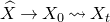 $\widehat{X} \rightarrow X_0 \rightsquigarrow X_t$
be a conifold transition. There exists a family of smooth metrics
$\widehat{X} \rightarrow X_0 \rightsquigarrow X_t$
be a conifold transition. There exists a family of smooth metrics $(\widehat{X},\widehat{g}_a,\widehat{H}_a)$
for
$(\widehat{X},\widehat{g}_a,\widehat{H}_a)$
for $0<a<1$
and
$0<a<1$
and $(X_t,g_t,H_t)$
for
$(X_t,g_t,H_t)$
for $0<|t|<\epsilon$
solving
$0<|t|<\epsilon$
solving
 \begin{equation*}d \omega^2=0, \quad F_H \wedge \omega^2= 0\end{equation*}
such that, as the parameters a and t are varied, the geometries $(X,\widehat{g}_a,\widehat{H}_a)$
and
$(X,\widehat{g}_a,\widehat{H}_a)$
and $(X_t,g_t,H_t)$
vary continuously in the Gromov–Hausdorff sense and
$(X_t,g_t,H_t)$
vary continuously in the Gromov–Hausdorff sense and
 \begin{align*} (\widehat{X}, \widehat{g}_a)& \rightarrow (X_0,d_{g_0}) \leftarrow (X_t,g_t), \nonumber\\ (\widehat{X}, \widehat{H}_a) &\rightarrow (X_0,d_{H_0}) \leftarrow (X_t,H_t)\end{align*}
as $a, t \rightarrow 0$
in the Gromov–Hausdorff topology. The length spaces
$a, t \rightarrow 0$
in the Gromov–Hausdorff topology. The length spaces $(X_0,d_{g_0})$
and
$(X_0,d_{g_0})$
and $(X_0,d_{H_0})$
are induced by a limiting Hermitian Yang–Mills structure on
$(X_0,d_{H_0})$
are induced by a limiting Hermitian Yang–Mills structure on $((X_0)_{\mathrm{reg}},\omega_0,H_0)$
.
$((X_0)_{\mathrm{reg}},\omega_0,H_0)$
.
Our proof begins by analyzing the local models, which are Kähler Ricci-flat metrics on the small resolution and smoothing of the affine cone $\{ \sum z_i^2 = 0 \} \subset \mathbb{C}^4$
. Once the local models are understood, we move on to the global balanced and Hermitian Yang–Mills structures (g,H). These global metrics add non-Kähler corrections to the Kähler Ricci-flat local models by solving a partial differential equation (PDE) on the global compact manifold: for the balanced metrics
$\{ \sum z_i^2 = 0 \} \subset \mathbb{C}^4$
. Once the local models are understood, we move on to the global balanced and Hermitian Yang–Mills structures (g,H). These global metrics add non-Kähler corrections to the Kähler Ricci-flat local models by solving a partial differential equation (PDE) on the global compact manifold: for the balanced metrics $\omega$
, the PDE involves the fourth-order Kodaira–Spencer operator, while for the metric H, the PDE is the Hermitian Yang–Mills equation. Our analysis relies on suitable estimates for these equations along degenerations. To obtain continuity at
$\omega$
, the PDE involves the fourth-order Kodaira–Spencer operator, while for the metric H, the PDE is the Hermitian Yang–Mills equation. Our analysis relies on suitable estimates for these equations along degenerations. To obtain continuity at $a=t=0$
, the main step is to obtain diameter bounds tending to zero near the singular points, and the general approach is in the style of Song and Weinkove [Reference Song and WeinkoveSW13, Reference Song and WeinkoveSW14], where exceptional sets are contracted along a sequence of metrics.
$a=t=0$
, the main step is to obtain diameter bounds tending to zero near the singular points, and the general approach is in the style of Song and Weinkove [Reference Song and WeinkoveSW13, Reference Song and WeinkoveSW14], where exceptional sets are contracted along a sequence of metrics.
2. Preliminaries
2.1 The Gromov–Hausdorff topology
The Gromov–Hausdorff topology was introduced in 1975 by Edwards [Reference EdwardsEdw75], and was then independently rediscovered by Gromov in the 1980s. Since then, it has been an indispensable tool in geometry. There has been growing interest in applications of the Gromov–Hausdorff topology to Calabi–Yau manifolds starting with the work of Gross and Wilson [Reference Gross and WilsonGW00], and we note in particular the use of this topology in studying the continuity of conifold transitions of Calabi–Yau threefolds (see [Reference Rong and ZhangRZ11a, Reference Ruan and ZhangRZ11b, Reference SongSon15]).
We will now introduce certain definitions and notions pertaining to Gromov–Hausdorff convergence of compact metric spaces. Other sources for this material include e.g. [Reference Burago, Burago and IvanovBBI01, Reference GromovGro07, Reference Gross and WilsonGW00, Reference EdwardsEdw75, Reference PetersenPet06]. We will implicitly assume that all our metric spaces in this section are compact, though generalizations exist for the non-compact case (cf. pointed Gromov–Hausdorff convergence).
Let (X,d) be a compact metric space. For $A \subseteq X$
and
$A \subseteq X$
and $\epsilon \gt 0$
, we set
$\epsilon \gt 0$
, we set
 \begin{equation*} B_\epsilon(A) = \bigcup_{x \in A} B_\epsilon(x),\end{equation*}
where $B_\epsilon(x) = \{x' \in X \mid d(x',x) \lt \epsilon\}$
is the ball of radius
$B_\epsilon(x) = \{x' \in X \mid d(x',x) \lt \epsilon\}$
is the ball of radius $\epsilon$
around x.
$\epsilon$
around x.
Definition 2.1. Let $(X,d_X)$
and
$(X,d_X)$
and $(Y,d_Y)$
be compact metric spaces and
$(Y,d_Y)$
be compact metric spaces and $\epsilon \gt 0$
. A map
$\epsilon \gt 0$
. A map $f \colon X \rightarrow Y$
is called an
$f \colon X \rightarrow Y$
is called an $\epsilon$
-isometry if
$\epsilon$
-isometry if
-
(i) $|d_X(x,x') - d_Y(f(x),f(x'))| \lt \epsilon$
for all
$x,x' \in X$
; and
$|d_X(x,x') - d_Y(f(x),f(x'))| \lt \epsilon$
for all
$x,x' \in X$
; and -
(ii)
$Y \subseteq B_\epsilon(f(X))$
.



In general, $\epsilon$
-isometries need not be injective or even continuous.
$\epsilon$
-isometries need not be injective or even continuous.
Definition 2.2. The Gromov–Hausdorff distance $d_{\mathrm{GH}}$
between two compact metric spaces
$d_{\mathrm{GH}}$
between two compact metric spaces $(X,d_X)$
and
$(X,d_X)$
and $(Y,d_Y)$
is
$(Y,d_Y)$
is
 \begin{equation*} d_{\mathrm{GH}}(X,Y) = \inf \{ \epsilon \gt 0 \mid \text{there exist } \epsilon\text{-isometries } f_1 \colon X \rightarrow Y, \, f_2 \colon Y \rightarrow X \}.\end{equation*}
The Gromov–Hausdorff distance $d_{\mathrm{GH}}$
defines a metric, and hence a topology, on the set
$d_{\mathrm{GH}}$
defines a metric, and hence a topology, on the set $\mathcal{M}$
of isometry classes of compact metric spaces.
$\mathcal{M}$
of isometry classes of compact metric spaces.
Remark 3. We note that only one of the $\epsilon$
-isometries in the previous definition is required as, given an
$\epsilon$
-isometries in the previous definition is required as, given an $\epsilon$
-isometry
$\epsilon$
-isometry $f_1 \colon X \rightarrow Y$
, one can construct a
$f_1 \colon X \rightarrow Y$
, one can construct a $3\epsilon$
-isometry
$3\epsilon$
-isometry $f_2 \colon Y \rightarrow X$
. This in essence scales the Gromov–Hausdorff metric
$f_2 \colon Y \rightarrow X$
. This in essence scales the Gromov–Hausdorff metric $d_{\mathrm{GH}}$
by a factor of 3, but both generate the same topology on
$d_{\mathrm{GH}}$
by a factor of 3, but both generate the same topology on $\mathcal{M}$
.
$\mathcal{M}$
.
2.2 Conifold transitions
Conifold transitions describe a process wherein one Calabi–Yau threefold is gradually deformed into another, passing through an intermediate space having cone singularities (i.e. a conifold).
We briefly review certain facts about the geometry of conifold transitions. The exposition here will follow [Reference Collins, Picard and YauCPY24, Reference Fu, Li and YauFLY12, Reference FriedmanFri91]. We begin with some definitions to fix the setup of this document.
Definition 2.3. A Kähler Calabi–Yau threefold $\widehat{X}$
is a compact complex manifold of complex dimension 3 with finite fundamental group, trivial canonical bundle, and admitting a Kähler metric.
$\widehat{X}$
is a compact complex manifold of complex dimension 3 with finite fundamental group, trivial canonical bundle, and admitting a Kähler metric.
Definition 2.4. A $(-1,-1)$
-curve
$(-1,-1)$
-curve $E \in \widehat{X}$
is a smooth rational curve
$E \in \widehat{X}$
is a smooth rational curve $E \simeq \mathbb{P}^1$
such that the normal bundle
$E \simeq \mathbb{P}^1$
such that the normal bundle $N_{E/\widehat{X}} \simeq \mathcal{O}(-1) \oplus \mathcal{O}(-1)$
.
$N_{E/\widehat{X}} \simeq \mathcal{O}(-1) \oplus \mathcal{O}(-1)$
.
Around a $(-1,-1)$
-curve E, there exists an open neighborhood
$(-1,-1)$
-curve E, there exists an open neighborhood $\widehat{U}$
which is biholomorphic to a neighborhood of the zero section in the total space of the bundle
$\widehat{U}$
which is biholomorphic to a neighborhood of the zero section in the total space of the bundle
 \begin{equation*} \widehat{V} = \mathcal{O}(-1) \oplus \mathcal{O}(-1) \rightarrow \mathbb{P}^1.\end{equation*}
Given a collection of disjoint $(-1,-1)$
-curves
$(-1,-1)$
-curves $\{ E_i \} \subset \widehat{X}$
, we may contract them to points by a blowdown map
$\{ E_i \} \subset \widehat{X}$
, we may contract them to points by a blowdown map $\pi \colon \widehat{X} \rightarrow X_0$
, where
$\pi \colon \widehat{X} \rightarrow X_0$
, where $X_0$
is a singular space with isolated singular points at
$X_0$
is a singular space with isolated singular points at $s_i = \pi(E_i)$
.
$s_i = \pi(E_i)$
.
In more detail, we identify a neighborhood of $E_i$
with the model space
$E_i$
with the model space $\widehat{V}$
and the blowdown map
$\widehat{V}$
and the blowdown map $\pi$
sends the complement of the zero section biholomorphically to the complement of the origin in the conifold
$\pi$
sends the complement of the zero section biholomorphically to the complement of the origin in the conifold
 \begin{equation*} V_0 = \Big\{z \in \mathbb{C}^4 \mid \sum_i z_i^2 = 0 \Big\}.\end{equation*}
This map $\pi$
can be holomorphically extended to all of
$\pi$
can be holomorphically extended to all of $\widehat{V}$
by sending the zero section to the origin in
$\widehat{V}$
by sending the zero section to the origin in $V_0$
. The map
$V_0$
. The map $\pi$
near
$\pi$
near $E_i$
can be made explicit and we give the expression later in (5). The result is that
$E_i$
can be made explicit and we give the expression later in (5). The result is that $X_0$
has isolated ordinary double-point (ODP) singularities
$X_0$
has isolated ordinary double-point (ODP) singularities $s_i$
with local neighborhoods biholomorphic to
$s_i$
with local neighborhoods biholomorphic to $0 \in V_0$
.
$0 \in V_0$
.
We next discuss how to smooth the singular space $X_0$
by deforming its holomorphic structure. The local model is a singular variety
$X_0$
by deforming its holomorphic structure. The local model is a singular variety $V_0$
which can be smoothed by considering the space
$V_0$
which can be smoothed by considering the space
 \begin{equation*} \mathcal{V} = \Big\{ (z,t) \in \mathbb{C}^4 \times \mathbb{C} \mid \sum_i z_i^2 = t \Big\}.\end{equation*}
The fiber over t is denoted $V_t$
(considered as a subset of
$V_t$
(considered as a subset of $\mathbb{C}^4$
) and is smooth for all
$\mathbb{C}^4$
) and is smooth for all $t \neq 0$
,
$t \neq 0$
,
 \begin{equation*} V_t = \Big\{z \in \mathbb{C}^4 \mid \sum_i z_i^2 = t \Big\}.\end{equation*}
This is the local model, depicted in Figure 1, which we would like to achieve globally on $X_0$
. A result of R. Friedman [Reference FriedmanFri86] gives a condition describing the existence of a smoothing.
$X_0$
. A result of R. Friedman [Reference FriedmanFri86] gives a condition describing the existence of a smoothing.
Local model of a conifold transition.

Theorem 2.5 (Friedman [Reference FriedmanFri86, Reference FriedmanFri91]). Suppose $\widehat{X}$
is a Kähler Calabi–Yau threefold and let
$\widehat{X}$
is a Kähler Calabi–Yau threefold and let $E_1,\ldots,E_k$
be disjoint
$E_1,\ldots,E_k$
be disjoint $(-1,-1)$
-curves. Let
$(-1,-1)$
-curves. Let $\pi$
be the blowdown map that contracts each
$\pi$
be the blowdown map that contracts each $E_i$
, resulting in the singular space
$E_i$
, resulting in the singular space $X_0$
with ODP singularities
$X_0$
with ODP singularities $s_i = \pi(E_i)$
. There exists a first-order deformation of
$s_i = \pi(E_i)$
. There exists a first-order deformation of $X_0$
smoothing each
$X_0$
smoothing each $s_i$
if and only if there exists a relation
$s_i$
if and only if there exists a relation
 \begin{equation*} \sum_i \lambda_i [E_i] = 0 \text{ in } H^2(\widehat{X},\mathbb{R})\end{equation*}
with each $\lambda_i \neq 0$
.
$\lambda_i \neq 0$
.
It has been shown that the first-order deformations from the above theorem integrate to genuine smoothings; see [Reference KawamataKaw92, Reference RanRan92, Reference TianTia92]. Thus, assuming the condition of Theorem 2.5 holds, we get a holomorphic family
 \begin{equation*} \mu \colon \mathcal{X} \rightarrow \Delta,\end{equation*}
where $\Delta \subset \mathbb{C}$
denotes the unit complex disc such that the fibers
$\Delta \subset \mathbb{C}$
denotes the unit complex disc such that the fibers $X_t = \mu^{-1}(t)$
are smooth complex manifolds for
$X_t = \mu^{-1}(t)$
are smooth complex manifolds for $t \neq 0$
and
$t \neq 0$
and $X_0 = \mu^{-1}(0)$
. A result of Kas and Schlessinger [Reference Kas and SchlessingerKS72] shows that the family
$X_0 = \mu^{-1}(0)$
. A result of Kas and Schlessinger [Reference Kas and SchlessingerKS72] shows that the family $\mathcal{X}$
is locally biholomorphic to the model
$\mathcal{X}$
is locally biholomorphic to the model $\mathcal{V}$
near each ODP. It can be shown that the complex manifolds
$\mathcal{V}$
near each ODP. It can be shown that the complex manifolds $X_t$
have trivial canonical bundle; see [Reference FriedmanFri86] for an algebraic proof or [Reference Collins, Gukov, Picard and YauCGP+23] for a differential geometric proof.
$X_t$
have trivial canonical bundle; see [Reference FriedmanFri86] for an algebraic proof or [Reference Collins, Gukov, Picard and YauCGP+23] for a differential geometric proof.
Definition 2.6. Let $\widehat{X}$
be a Kähler Calabi–Yau threefold. A conifold transition starting from
$\widehat{X}$
be a Kähler Calabi–Yau threefold. A conifold transition starting from $\widehat{X}$
, denoted
$\widehat{X}$
, denoted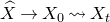 $\widehat{X} \rightarrow X_0 \rightsquigarrow X_t$
, consists of a holomorphic map
$\widehat{X} \rightarrow X_0 \rightsquigarrow X_t$
, consists of a holomorphic map $\pi \colon \widehat{X} \rightarrow X_0$
and a family
$\pi \colon \widehat{X} \rightarrow X_0$
and a family $\mu \colon \mathcal{X} \rightarrow \Delta$
with
$\mu \colon \mathcal{X} \rightarrow \Delta$
with $X_0 = \mu^{-1}(0)$
such that:
$X_0 = \mu^{-1}(0)$
such that:
-
(i) the map
$\pi \colon \widehat{X} \rightarrow X_0$
contracts a collection of disjoint
$(-1,-1)$
-curves
$E_1,\ldots,E_k \subseteq \widehat{X}$
to isolated ODP singularities
$s_1,\ldots,s_k \in X_0$
and
$\pi$
is a biholomorphism between
$\widehat{X} \setminus (E_1 \cup \dots \cup E_k)$
and
$X_0 \setminus \{s_1,\ldots,s_k\}$
; and -
(ii) the total space
$\mathcal{X}$
is a smooth complex fourfold with a proper flat map
$\mu \colon \mathcal{X} \rightarrow \Delta$
, where
$X_0 = \mu^{-1}(0)$
and
$X_t = \mu^{-1}(t)$
are smooth complex manifolds for
$t \neq 0$
.









It is known that the Kähler condition is not necessarily preserved along a conifold transition. For a concrete example, suppose $\widehat{X}$
is a quintic threefold and choose a pair of disjoint
$\widehat{X}$
is a quintic threefold and choose a pair of disjoint $(-1,-1)$
-curves
$(-1,-1)$
-curves $E_1$
,
$E_1$
, $E_2$
(for the existence of such curves, see e.g. [Reference ClemensCle83]). Since
$E_2$
(for the existence of such curves, see e.g. [Reference ClemensCle83]). Since $b_2(\widehat{X})=1$
, these satisfy Friedman’s condition. Thus, a conifold transition exists, and since the generator of second homology has been sent to a point, we have
$b_2(\widehat{X})=1$
, these satisfy Friedman’s condition. Thus, a conifold transition exists, and since the generator of second homology has been sent to a point, we have $b_2(X_t)=0$
. We see that
$b_2(X_t)=0$
. We see that $X_t$
may not support any Kähler metric, even if the initial
$X_t$
may not support any Kähler metric, even if the initial $\widehat{X}$
is a projective threefold. For further examples of Kähler to non-Kähler conifold transitions, we refer to [Reference FriedmanFri91, Reference Lu and TianLT94], and for the study of Hodge structures through such a process, see [Reference FriedmanFri19].
$\widehat{X}$
is a projective threefold. For further examples of Kähler to non-Kähler conifold transitions, we refer to [Reference FriedmanFri91, Reference Lu and TianLT94], and for the study of Hodge structures through such a process, see [Reference FriedmanFri19].
To geometrize the parameter space of Calabi–Yau threefolds connected by conifold transitions, we must therefore look for special non-Kähler metrics. This program was initiated by Fu, Li and Yau [Reference Fu, Li and YauFLY12]. The inspiration comes from supersymmetric constraints in string theory. Kähler Calabi–Yau metrics satisfy the system of supersymmetric constraints when the H-flux is taken to be zero [Reference Candelas, Horowitz, Strominger and WittenCHS+85]. As pointed out in e.g. [Reference ReidRei87], Chapter 4 of [Reference HubschHub92] or §6 of [Reference Candelas, de la Ossa, Green and ParkesCdlOG+91], a degeneration and resolution may connect a Kähler threefold to a non-Kähler space, and so it is necessary to look for more general solutions to the supersymmetric constraints with non-zero H-flux. These constraints were worked out by Strominger [Reference StromingerStr86] and imply the following two equations.
-
– X admits a balanced metric
$\omega$
. A Hermitian metric g on
$T^{1,0}X$
over a complex manifold X of dimension n is balanced if (2)Here,
\begin{equation} d \omega^{n-1} = 0. \end{equation}
$\omega$
is the (1,1)-form associated to g via
$\omega= \sqrt{-1} g_{j \bar{k}} dz^j \wedge d \bar{z}^k$
. Various properties of balanced metrics were explored by Michelsohn [Reference MichelsohnMic82].
-
– X admits a Hermitian Yang–Mills metric. A Hermitian metric H on
$T^{1,0}X$
is Hermitian Yang–Mills with respect to a balanced metric
$\omega$
if (3)The Chern curvature of a metric H is denoted by
\begin{equation} F \wedge \omega^{n-1} = 0. \end{equation}
$F \in \Lambda^{1,1}(\textrm{End} \, T^{1,0}X)$
, and is given by
$F=\bar{\partial}(\partial H H^{-1})$
. The criterion for the solvability of this equation over a general holomorphic bundle is given by the Donaldson–Uhlenbeck–Yau theorem [Reference DonaldsonDon85, Reference Uhlenbeck and YauUY86] in the Kähler case, with an extension by Li and Yau [Reference Li and YauLY87] for non-Kähler metrics.







When X is a Kähler threefold, Yau’s theorem [Reference YauYau78] gives the existence of a Kähler Ricci-flat metric $g_\textrm{CY}$
. The above equations are then solved with
$g_\textrm{CY}$
. The above equations are then solved with $g=H=g_\textrm{CY}$
. More generally, let
$g=H=g_\textrm{CY}$
. More generally, let $X_t$
be a complex manifold connected to a Kähler threefold via a conifold transition
$X_t$
be a complex manifold connected to a Kähler threefold via a conifold transition $\widehat{X} \rightarrow X_0 \rightsquigarrow X_t$
. The main results of [Reference Fu, Li and YauFLY12] and [Reference Collins, Picard and YauCPY24] give the existence of a pair (g,H) solving the supersymmetric equations (2) and (3).
$\widehat{X} \rightarrow X_0 \rightsquigarrow X_t$
. The main results of [Reference Fu, Li and YauFLY12] and [Reference Collins, Picard and YauCPY24] give the existence of a pair (g,H) solving the supersymmetric equations (2) and (3).
Remark 4. The Hermitian Yang–Mills equation may, in principle, also be solved over an auxiliary gauge bundle E, but the mechanism under which a conifold transition creates a stable holomorphic vector bundle $E_t \rightarrow X_t$
is not understood, except for the case at hand, which is when
$E_t \rightarrow X_t$
is not understood, except for the case at hand, which is when $E_t = T^{1,0} X_t$
. There is a proposal by Anderson, Brodie and Gray [Reference Anderson, Brodie and GrayABG23] in the string-theory literature on how such general bundles may appear on the other side. There is also work of Chuan [Reference ChuanChu12] on the Hermitian Yang–Mills equation on a gauge bundle E with the additional assumption that E is locally a trivial bundle through the singularities of a conifold transition.
$E_t = T^{1,0} X_t$
. There is a proposal by Anderson, Brodie and Gray [Reference Anderson, Brodie and GrayABG23] in the string-theory literature on how such general bundles may appear on the other side. There is also work of Chuan [Reference ChuanChu12] on the Hermitian Yang–Mills equation on a gauge bundle E with the additional assumption that E is locally a trivial bundle through the singularities of a conifold transition.
In the remainder of this preliminary section, we recall various metrics which can be defined both globally and on the local models, and state the main results of this paper, which state that conifold transitions, when bestowed with these metrics, describe a continuous path in $\mathcal{M}$
with respect to the Gromov–Hausdorff topology.
$\mathcal{M}$
with respect to the Gromov–Hausdorff topology.
2.3 Metrics on small resolutions
2.3.1 Candelas–de la Ossa metrics on the local model.
Consider the space $\widehat{V}$
, which is the total space of the bundle
$\widehat{V}$
, which is the total space of the bundle
 \begin{equation*} \widehat{V} = \mathcal{O}(-1) \oplus \mathcal{O}(-1) \rightarrow \mathbb{P}^1.\end{equation*}
On this space, we have two trivializations
 \begin{equation*} (U, (\lambda, u,v)) \text{ and } (U', (\lambda', u', v')),\end{equation*}
with transition functions given by
 \begin{equation*} \lambda' = \lambda^{-1}, \, u' = \lambda u, \, v' = \lambda v.\end{equation*}
Note that $\lambda$
is the coordinate on the base space
$\lambda$
is the coordinate on the base space $\mathbb{P}^1$
, while u,v are fiber coordinates.
$\mathbb{P}^1$
, while u,v are fiber coordinates.
It will be convenient to define the well-defined radius function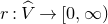 $r: \widehat{V} \rightarrow [0,\infty)$
given by
$r: \widehat{V} \rightarrow [0,\infty)$
given by
 \begin{equation*} r(\lambda, u, v) = (1 + |\lambda|^2)^{{1}/{3}} (|u|^2 + |v|^2)^{{1}/{3}}.\end{equation*}
Without the power of $\tfrac{1}{3}$
, this function measures the distance squared from a point to the zero section
$\tfrac{1}{3}$
, this function measures the distance squared from a point to the zero section $E \simeq \mathbb{P}^1$
along the fibers using the Fubini–Study metric
$E \simeq \mathbb{P}^1$
along the fibers using the Fubini–Study metric $\widehat{\omega}_{FS}$
. The power is introduced so that this radius function coincides with the radius of the Calabi–Yau cone metric on the blowdown, and this will be discussed later.
$\widehat{\omega}_{FS}$
. The power is introduced so that this radius function coincides with the radius of the Calabi–Yau cone metric on the blowdown, and this will be discussed later.
The space $(\widehat{V}, r)$
is also equipped with a family of scaling maps. Namely, for
$(\widehat{V}, r)$
is also equipped with a family of scaling maps. Namely, for $R\gt0$
, we have the map
$R\gt0$
, we have the map $S_R: \widehat{V} \rightarrow \widehat{V}$
given by
$S_R: \widehat{V} \rightarrow \widehat{V}$
given by
 \begin{equation*} S_R(\lambda,u,v) = (\lambda,R^{{3}/{2}}u, R^{{3}/{2}} v).\end{equation*}
The radius behaves as it should under the scaling, as we have
 \begin{equation*} r \circ S_R = R \cdot r.\end{equation*}
In [Reference Candelas and de la OssaCdlO90], Candelas and de la Ossa look for a Kähler Ricci-flat metric $\widehat{\omega}_{\mathrm{co},1}$
on
$\widehat{\omega}_{\mathrm{co},1}$
on $\widehat{V}$
of the form
$\widehat{V}$
of the form
 \begin{equation*} \widehat{\omega}_{\mathrm{co},1} = \sqrt{-1} \partial \overline{\partial} f(r^3) + 4 \widehat{\omega}_{\mathrm{FS}},\end{equation*}
where $\widehat{\omega}_{\mathrm{FS}}$
is the Fubini–Study metric on
$\widehat{\omega}_{\mathrm{FS}}$
is the Fubini–Study metric on $\mathbb{P}^1$
, and
$\mathbb{P}^1$
, and $f(x)=f(r^3)$
is a smooth function. They show that imposing the condition of Kähler Ricci-flatness yields the following first-order ODE for f:
$f(x)=f(r^3)$
is a smooth function. They show that imposing the condition of Kähler Ricci-flatness yields the following first-order ODE for f:
 \begin{equation*}x(f'(x))^3+6(f'(x))^2=1.\end{equation*}
The solution admits an expansion [Reference Collins, Picard and YauCPY24] for $x \gg 1$
given in terms of
$x \gg 1$
given in terms of $r=x^{{{1}/{3}}}$
by
$r=x^{{{1}/{3}}}$
by
 \begin{equation*}f =c_0 r^2 + c_1 \log r + c_2 r^{-2} + c_3 r^{-4} + \cdots\end{equation*}
for constants $c_0, c_1, c_2, \ldots.$
Thus, after rescaling
$c_0, c_1, c_2, \ldots.$
Thus, after rescaling $\widehat{\omega}_{\mathrm{co},1}$
such that
$\widehat{\omega}_{\mathrm{co},1}$
such that $c_0 = {\tfrac{1}{2}}$
, we have the following expansion for large radius
$c_0 = {\tfrac{1}{2}}$
, we have the following expansion for large radius $r \gg 1$
:
$r \gg 1$
:
 \begin{equation} \widehat{\omega}_{\mathrm{co},1} - \tfrac{1}{2} \sqrt{-1} \partial \bar{\partial} r^2 = c_{-1} \widehat{\omega}_{\mathrm{FS}} + c_1 \sqrt{-1} \partial \bar{\partial} \log r + c_2 \sqrt{-1} \partial \overline{\partial} r^{-2} + c_3 \sqrt{-1} \partial \overline{\partial} r^{-4} + \cdots.\end{equation}
Next, we note that the space $\widehat{V}$
can be regarded as a small blowup of the space
$\widehat{V}$
can be regarded as a small blowup of the space
 \begin{equation*} V_0 = \Big\{ z \in \mathbb{C}^4 \mid \sum_i z_i^2 = 0 \Big\}.\end{equation*}
There is a (scaled) blowdown map $\pi: \widehat{V} \rightarrow V_0$
such that
$\pi: \widehat{V} \rightarrow V_0$
such that $\pi^{-1}(0)$
is the zero section
$\pi^{-1}(0)$
is the zero section $E=\{r=0\}$
, and the restriction
$E=\{r=0\}$
, and the restriction
 \begin{equation*} \pi: \hat{V} \setminus E \rightarrow V_0 \setminus \{ 0 \}\end{equation*}
is biholomorphic. The map $\pi$
has the explicit expression
$\pi$
has the explicit expression
 \begin{equation} \pi (\lambda, u, v) = \bigg( \frac{\lambda v + u}{\sqrt{2}}, -\sqrt{-1} \cdot \frac{\lambda v - u}{\sqrt{2}}, -\sqrt{-1} \cdot \frac{v + \lambda u}{\sqrt{2}}, -\frac{v - \lambda u}{\sqrt{2}} \bigg)\!.\end{equation}
Likewise, away from the singularity at the origin, we can see that
 \begin{equation*} \pi^{-1} (z_1, z_2, z_3, z_4) = \bigg( \frac{z_1 - \sqrt{-1} z_2}{\sqrt{2}}, \frac{\sqrt{-1} (z_3 + \sqrt{-1} z_4)}{\sqrt{2}}, \sqrt{-1} \cdot \frac{z_3 - \sqrt{-1} z_4}{z_1 - \sqrt{-1} z_2} \bigg)\!.\end{equation*}
The function r on $\widehat{V}$
becomes
$\widehat{V}$
becomes $\| z \|^{{{2}/{3}}}$
on
$\| z \|^{{{2}/{3}}}$
on $V_0$
via the identification
$V_0$
via the identification $\pi$
, in the sense that
$\pi$
, in the sense that $r(\lambda, u, v) = \| \pi (\lambda, u, v)\|^{{{2}/{3}}}$
. For this reason, we will also denote
$r(\lambda, u, v) = \| \pi (\lambda, u, v)\|^{{{2}/{3}}}$
. For this reason, we will also denote
 \begin{equation*}r = \| z \|^{{2}/{3}} , \quad r: V_0 \rightarrow [0,\infty).\end{equation*}
The space $V_0$
admits a Calabi–Yau cone metric
$V_0$
admits a Calabi–Yau cone metric
 \begin{equation*} \omega_{\mathrm{co},0} = \tfrac{1}{2} \sqrt{-1} \partial \bar{\partial} r^2.\end{equation*}
We briefly discuss the cone-metric geometry on $(V_0, \omega_{\mathrm{co},0})$
. Observe that
$(V_0, \omega_{\mathrm{co},0})$
. Observe that $V_0$
is closed under scalar multiplication and addition, so that
$V_0$
is closed under scalar multiplication and addition, so that $V_0$
is a cone. The metric
$V_0$
is a cone. The metric $\omega_{\mathrm{co},0}$
is well known [Reference Candelas and de la OssaCdlO90] to be Kähler Ricci-flat and is a cone metric over the link
$\omega_{\mathrm{co},0}$
is well known [Reference Candelas and de la OssaCdlO90] to be Kähler Ricci-flat and is a cone metric over the link
 \begin{equation*} L = \{z \in V_0 \mid r(z) = 1\},\end{equation*}
and we may write
 \begin{equation} g_{\mathrm{co},0} = dr \otimes dr + r^2 \cdot g_L,\end{equation}
where $g_L$
is the pullback of a metric on L.
$g_L$
is the pullback of a metric on L.
The link L is $S^3 \times S^2$
. To see this, we express the defining condition
$S^3 \times S^2$
. To see this, we express the defining condition $\sum_i z_i^2 = 0$
of
$\sum_i z_i^2 = 0$
of $V_0$
in real coordinates
$V_0$
in real coordinates $x_i, y_i$
such that
$x_i, y_i$
such that $z_i = x_i + \sqrt{-1}y_i$
for each
$z_i = x_i + \sqrt{-1}y_i$
for each $i \in \{1,2,3,4\}$
. We obtain
$i \in \{1,2,3,4\}$
. We obtain
 \[0 = \| x \|^2 - \| y \|^2 +2\sqrt{-1}\langle x, y \rangle, \]
where $x=(x_1,x_2,x_3,x_4) \in \mathbb{R}^4$
and
$x=(x_1,x_2,x_3,x_4) \in \mathbb{R}^4$
and $y=(y_1,y_2,y_3,y_4) \in \mathbb{R}^4$
. Expressed in these terms,
$y=(y_1,y_2,y_3,y_4) \in \mathbb{R}^4$
. Expressed in these terms, $V_0$
is the set of all
$V_0$
is the set of all $(x,y) \in \mathbb{R}^8 \cong \mathbb{R}^4 \oplus \mathbb{R}^4$
on which
$(x,y) \in \mathbb{R}^8 \cong \mathbb{R}^4 \oplus \mathbb{R}^4$
on which $\| x \| = \| y \|$
and
$\| x \| = \| y \|$
and $\langle x, y \rangle = 0$
. Fixing
$\langle x, y \rangle = 0$
. Fixing $r^3=\| x \|^2 + \| y \|^2=2$
implies that
$r^3=\| x \|^2 + \| y \|^2=2$
implies that $\| x \|=\| y \|=1$
. In particular, we have
$\| x \|=\| y \|=1$
. In particular, we have $x \in S^3 \subset \mathbb{R}^4$
. Then, for each such choice of x, the conditions
$x \in S^3 \subset \mathbb{R}^4$
. Then, for each such choice of x, the conditions $\langle x, y \rangle=0$
and
$\langle x, y \rangle=0$
and $\| y \| = 1$
imply that y is in the unit 2-sphere centered at 0 in the tangent space
$\| y \| = 1$
imply that y is in the unit 2-sphere centered at 0 in the tangent space $T_x S^3$
. Thus, the set
$T_x S^3$
. Thus, the set $\{z \in V_0 \mid r(z)=2^{{{1}/{3}}}\}$
is diffeomorphic to the unit-sphere bundle contained in the tangent bundle
$\{z \in V_0 \mid r(z)=2^{{{1}/{3}}}\}$
is diffeomorphic to the unit-sphere bundle contained in the tangent bundle $TS^3$
, which is trivial. Thus,
$TS^3$
, which is trivial. Thus, $\{z \in V_0 \mid r(z)=2^{{{1}/{3}}}\} \cong S^3 \times S^2$
, and by rescaling we have
$\{z \in V_0 \mid r(z)=2^{{{1}/{3}}}\} \cong S^3 \times S^2$
, and by rescaling we have $L \cong S^3 \times S^2$
as well.
$L \cong S^3 \times S^2$
as well.
Returning to $(\widehat{V}, \widehat{g}_{\mathrm{co},1})$
, we can rescale the area of the zero section
$(\widehat{V}, \widehat{g}_{\mathrm{co},1})$
, we can rescale the area of the zero section $E \simeq \mathbb{P}^1$
to obtain a 1-parameter family of metrics. We will refer to this family of metrics as the Candelas–de la Ossa metrics
$E \simeq \mathbb{P}^1$
to obtain a 1-parameter family of metrics. We will refer to this family of metrics as the Candelas–de la Ossa metrics $\widehat{g}_{\mathrm{co},a}$
on the small resolution. The metrics
$\widehat{g}_{\mathrm{co},a}$
on the small resolution. The metrics $\widehat{g}_{\mathrm{co},a}$
satisfy the following important properties.
$\widehat{g}_{\mathrm{co},a}$
satisfy the following important properties.
-
(CO SR I) Normalization. For
$a \gt 0$
, we have
\begin{equation*} \widehat{g}_{\mathrm{co},a} = a^2 \cdot S_{a^{-1}}^* (\widehat{g}_{\mathrm{co},1}). \end{equation*}
-
(CO SR II) Asymptotically conical decay. There exists
$C \gt 0$
independent of a such that for all
$a \gt 0$
, The asymptotic decay can be derived from (4) for
\begin{equation*} |(\pi^{-1})^* (\widehat{g}_{\mathrm{co},a}) - g_{\mathrm{co},0}|_{g_{\mathrm{co},0}} \leq C a^2 r^{-2}. \end{equation*}
$a=1$
. Pulling back the estimate when
$a=1$
by
$S^*_a$
gives the estimate for general a. The estimate implies that the Candelas–de la Ossa metrics
$\widehat{g}_{\mathrm{co},a}$
converge uniformly to the cone metric
$g_{\mathrm{co},0}$
on compact sets away from the zero section E.


For $R\gt 0$
, we will denote by
$R\gt 0$
, we will denote by $\widehat{T}(R)$
the ‘tube’
$\widehat{T}(R)$
the ‘tube’
 \[\widehat{T}(R) := \{r \leq R\} \subseteq \widehat{V} \]
around the zero section $E \simeq \mathbb{P}^1$
. On the cone
$E \simeq \mathbb{P}^1$
. On the cone $V_0$
, we will analogously refer to the ‘disc’
$V_0$
, we will analogously refer to the ‘disc’
 \[D_0(R) := \{r \leq R\} \subseteq V_0 \]
of radius R around 0.
Let $\widehat{d}_{\mathrm{co},a}$
and
$\widehat{d}_{\mathrm{co},a}$
and $d_{\mathrm{co},0}$
denote the induced distance functions on
$d_{\mathrm{co},0}$
denote the induced distance functions on $\widehat{X}$
and
$\widehat{X}$
and $X_0$
by
$X_0$
by $\widehat{g}_{\mathrm{co},a}$
and
$\widehat{g}_{\mathrm{co},a}$
and $g_{\mathrm{co},0}$
, respectively. As warm-up for our proof of the convergence of metrics on the compact threefold, we will present a proof of convergence of the local models.
$g_{\mathrm{co},0}$
, respectively. As warm-up for our proof of the convergence of metrics on the compact threefold, we will present a proof of convergence of the local models.
Theorem 2.7. The spaces $( \widehat{T}(1),\widehat{d}_{\mathrm{co},a} )$
converge in the Gromov–Hausdorff topology as
$( \widehat{T}(1),\widehat{d}_{\mathrm{co},a} )$
converge in the Gromov–Hausdorff topology as $a \to 0$
to the space
$a \to 0$
to the space $(D_0(1), d_{\mathrm{co},0})$
.
$(D_0(1), d_{\mathrm{co},0})$
.
A proof of this fact also follows from the PDE estimates in [Reference Collins, Guo and TongCGT22] for general asymptotically conical Calabi–Yau metrics on small resolutions.
2.3.2 Balanced metrics on the small resolution.
Next, we state the properties that we will need from the Fu–Li–Yau metrics on the compact Calabi–Yau threefold $\widehat{X}$
. Let
$\widehat{X}$
. Let $\widehat{\omega}_\textrm{ CY}$
be a Kähler metric on the Kähler threefold
$\widehat{\omega}_\textrm{ CY}$
be a Kähler metric on the Kähler threefold $\widehat{X}$
. The Fu–Li–Yau gluing construction [Reference Fu, Li and YauFLY12] (see also [Reference Collins, Picard and YauCPY24] and [Reference ChuanChu12] for further details on
$\widehat{X}$
. The Fu–Li–Yau gluing construction [Reference Fu, Li and YauFLY12] (see also [Reference Collins, Picard and YauCPY24] and [Reference ChuanChu12] for further details on $\widehat{\omega}_{\mathrm{FLY},a}$
for
$\widehat{\omega}_{\mathrm{FLY},a}$
for $a \neq 0$
) produces a sequence of metrics
$a \neq 0$
) produces a sequence of metrics $\widehat{\omega}_{\mathrm{FLY},a}$
for
$\widehat{\omega}_{\mathrm{FLY},a}$
for $0 \leq a \leq 1$
such that
$0 \leq a \leq 1$
such that
 \begin{equation*} d \widehat{\omega}_{\mathrm{FLY},a}^2 = 0, \quad [\widehat{\omega}_{\mathrm{FLY},a}^2]=[\widehat{\omega}_\textrm{CY}^2] \in H^4(\widehat{X},\mathbb{R}).\end{equation*}
For the purposes of this paper, we will mainly make use of the two following properties.
-
(FLY SR I) Local model. There exists
$\delta\gt 0$
and
$R\gt 1$
such that for all
$0 \leq a \leq 1$
, we have Here, the function
\begin{equation*} \widehat{\omega}_{\mathrm{FLY},a}|_{ \{ r< \delta \}} = R \cdot \widehat{\omega}_{\mathrm{co},a}.\end{equation*}
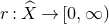
$r: \widehat{X} \rightarrow [0,\infty)$
extends the local functions r defined on a neighborhood of the curves
$E_i \subset \widehat{V}$
to the whole compact manifold
$\widehat{X}$
such that the set
$\{ r \lt \delta \}$
consists of small disjoint open neighborhoods containing the
$(-1,-1)$
-curves
$E_1, \dots, E_k$
.
-
(FLY SR II) Uniform convergence. For any compact set
$K \subset \widehat{X} \setminus ( E_1 \cup \dots \cup E_k)$
, the sequence
$\widehat{\omega}_{\mathrm{FLY},a}$
converges uniformly to
$\widehat{\omega}_{\mathrm{FLY},0}$
as
$a \rightarrow 0$
on K.







For each $E_i \simeq \mathbb{P}^1$
, these metrics satisfy
$E_i \simeq \mathbb{P}^1$
, these metrics satisfy
 \begin{equation} \int_{\mathbb{P}^1} \widehat{\omega}_{\mathrm{FLY},a} \rightarrow 0, \quad a \rightarrow 0.\end{equation}
The limiting metric $\widehat{\omega}_{\mathrm{FLY},0}$
is singular on the curves
$\widehat{\omega}_{\mathrm{FLY},0}$
is singular on the curves $E_1, \dots, E_k$
, and only defines a genuine metric on
$E_1, \dots, E_k$
, and only defines a genuine metric on $\widehat{X} \backslash (E_1 \cup \dots \cup E_k)$
.
$\widehat{X} \backslash (E_1 \cup \dots \cup E_k)$
.
Let $\pi: \widehat{X} \rightarrow X_0$
be the contraction of the curves, and let
$\pi: \widehat{X} \rightarrow X_0$
be the contraction of the curves, and let $s_i = \pi(E_i)$
be the singular points of
$s_i = \pi(E_i)$
be the singular points of $X_0$
. We will write
$X_0$
. We will write $(X_0)_\textrm{reg} = X_0 \backslash \{ s_1, \dots, s_k \}$
. Since
$(X_0)_\textrm{reg} = X_0 \backslash \{ s_1, \dots, s_k \}$
. Since $\widehat{X} \backslash (E_1 \cup \dots \cup E_k) \simeq (X_0)_\textrm{reg}$
, the limiting metric
$\widehat{X} \backslash (E_1 \cup \dots \cup E_k) \simeq (X_0)_\textrm{reg}$
, the limiting metric $\widehat{\omega}_{\mathrm{FLY},0}$
defines a Riemannian structure
$\widehat{\omega}_{\mathrm{FLY},0}$
defines a Riemannian structure $( (X_0)_{\mathrm{reg}}, \, \omega_{\mathrm{FLY},0} )$
with conical singularities. This induces a distance function
$( (X_0)_{\mathrm{reg}}, \, \omega_{\mathrm{FLY},0} )$
with conical singularities. This induces a distance function $d_{\mathrm{FLY},0}$
on
$d_{\mathrm{FLY},0}$
on $X_0$
.
$X_0$
.
This brings us to one of our main theorems.
Theorem 2.8. The compact metric spaces $(\widehat{X},\widehat{d}_{\mathrm{FLY},a})$
converge to
$(\widehat{X},\widehat{d}_{\mathrm{FLY},a})$
converge to $(X_0,d_{\mathrm{FLY},0})$
in the Gromov–Hausdorff topology as
$(X_0,d_{\mathrm{FLY},0})$
in the Gromov–Hausdorff topology as $a \to 0$
.
$a \to 0$
.
2.3.3 Hermitian Yang–Mills metrics on the small resolution.
We review the relevant properties of the sequence of Hermitian Yang–Mills metrics from [Reference Collins, Picard and YauCPY24]. Recall that our initial threefold $\widehat{X}$
is Kähler Calabi–Yau and simply connected. By dimensional considerations, an application of the de Rham decomposition theorem [Reference YauYau93] implies that
$\widehat{X}$
is Kähler Calabi–Yau and simply connected. By dimensional considerations, an application of the de Rham decomposition theorem [Reference YauYau93] implies that $(\widehat{X}, \widehat{\omega}_\textrm{CY})$
satisfies the stability condition
$(\widehat{X}, \widehat{\omega}_\textrm{CY})$
satisfies the stability condition
 \begin{equation*} \frac{1}{\text{rank}\,F} \int_{\widehat{X}} c_1(F) \wedge \widehat{\omega}^2_\textrm{CY} \lt 0\end{equation*}
for all torsion-free coherent proper subsheaves $F \subseteq T^{1,0}\widehat{X}$
. The Fu–Li–Yau metric
$F \subseteq T^{1,0}\widehat{X}$
. The Fu–Li–Yau metric $\widehat{\omega}_{\mathrm{FLY},a}$
and the Calabi–Yau metric
$\widehat{\omega}_{\mathrm{FLY},a}$
and the Calabi–Yau metric $\widehat{\omega}_\textrm{CY}$
have the same squared cohomology class, and so
$\widehat{\omega}_\textrm{CY}$
have the same squared cohomology class, and so
 \begin{equation*} \frac{1}{\text{rank}\,F} \int_{\widehat{X}} c_1(F) \wedge \widehat{\omega}^2_{\mathrm{FLY},a} \lt 0.\end{equation*}
It follows that $T^{1,0}\widehat{X}$
is stable with respect to each of the Fu–Li–Yau metrics. The Li–Yau generalization [Reference Li and YauLY87] of the Donaldson–Uhlenbeck–Yau theorem [Reference DonaldsonDon85, Reference Uhlenbeck and YauUY86] to Gauduchon metrics yields a family of metrics
$T^{1,0}\widehat{X}$
is stable with respect to each of the Fu–Li–Yau metrics. The Li–Yau generalization [Reference Li and YauLY87] of the Donaldson–Uhlenbeck–Yau theorem [Reference DonaldsonDon85, Reference Uhlenbeck and YauUY86] to Gauduchon metrics yields a family of metrics $\widehat{H}_a$
satisfying
$\widehat{H}_a$
satisfying
 \begin{equation} F_{\widehat{H}_a} \wedge \widehat{\omega}^2_{\mathrm{FLY},a} = 0, \quad \int_{\hat{X}} \log \frac{\det \widehat{H}_a}{\det \widehat{g}_{\mathrm{FLY},a}} \, d\textrm {vol}_{g_{\mathrm{FLY},a}} = 0.\end{equation}
This sequence $\widehat{H}_a$
satisfies the following estimates.
$\widehat{H}_a$
satisfies the following estimates.
Proposition 1 (Collins, Picard and Yau [Reference Collins, Picard and YauCPY24]). There exist constants $C, C_k \gt 0$
such that the Hermitian Yang–Mills metrics
$C, C_k \gt 0$
such that the Hermitian Yang–Mills metrics $\widehat{H}_a$
satisfy
$\widehat{H}_a$
satisfy
 \begin{align*} C^{-1} \cdot \widehat{g}_{\mathrm{FLY},a} &\leq \widehat{H}_a \leq C \cdot \widehat{g}_{\mathrm{FLY},a},\\ |\nabla^k \widehat{H}_a|_{\widehat{g}_{\mathrm{FLY},a}} &\leq C_k r^{-k}.\end{align*}
The metric $H_0$
on
$H_0$
on $(X_0)_{\mathrm{reg}}$
can be constructed as the limit of these metrics
$(X_0)_{\mathrm{reg}}$
can be constructed as the limit of these metrics $\widehat{H}_a$
. This was done in [Reference Collins, Picard and YauCPY24] by taking a subsequence of
$\widehat{H}_a$
. This was done in [Reference Collins, Picard and YauCPY24] by taking a subsequence of $\{ \widehat{H}_a \}$
. In Appendix A, we will show that these estimates imply that the full sequence converges on compact sets. Therefore, there exists a Hermitian Yang–Mills metric
$\{ \widehat{H}_a \}$
. In Appendix A, we will show that these estimates imply that the full sequence converges on compact sets. Therefore, there exists a Hermitian Yang–Mills metric $H_0$
over the singular space
$H_0$
over the singular space $X_0$
such that
$X_0$
such that
 \begin{equation*} F_{H_0} \wedge \omega^2_{\mathrm{FLY,0}} = 0, \quad C^{-1} \cdot g_{\mathrm{FLY},0} \leq H_0 \leq C \cdot g_{\mathrm{FLY},0}\end{equation*}
and for any compact set $K \subset \widehat{X} \setminus (E_1 \cup \dots \cup E_k)$
, the sequence
$K \subset \widehat{X} \setminus (E_1 \cup \dots \cup E_k)$
, the sequence $\widehat{H}_a$
converges uniformly to
$\widehat{H}_a$
converges uniformly to $H_0$
on K as
$H_0$
on K as $a \rightarrow 0$
. Going beyond compact subsets, we will prove the following.
$a \rightarrow 0$
. Going beyond compact subsets, we will prove the following.
Theorem 2.9. The compact metric spaces $(\widehat{X},\widehat{d}_{\widehat{H}_a})$
converge to
$(\widehat{X},\widehat{d}_{\widehat{H}_a})$
converge to $(X_0,d_{H_0})$
in the Gromov–Hausdorff topology as
$(X_0,d_{H_0})$
in the Gromov–Hausdorff topology as $a \to 0$
.
$a \to 0$
.
2.4 Metrics on smoothings
2.4.1 Candelas–de la Ossa metrics on the local model.
Next, for $t \neq 0$
, we consider the smooth submanifolds
$t \neq 0$
, we consider the smooth submanifolds $V_t \subset \mathbb{C}^4$
defined by
$V_t \subset \mathbb{C}^4$
defined by
 \begin{equation*} V_t = \Big\{ z \in \mathbb{C}^4 \mid \sum_i z_i^2 = t \Big\}.\end{equation*}
We have the usual norm $\|z\|^2$
on
$\|z\|^2$
on $V_t$
induced from
$V_t$
induced from $\mathbb{C}^4$
, given by
$\mathbb{C}^4$
, given by
 \begin{equation*} \|z\|^2 = \sum_{i=1}^4 |z_i|^2.\end{equation*}
Candelas and de la Ossa also constructed metrics $\omega_{\mathrm{co},t}$
on the smoothings
$\omega_{\mathrm{co},t}$
on the smoothings $V_t$
[Reference Candelas and de la OssaCdlO90]. The metrics are obtained by looking for potentials of the form
$V_t$
[Reference Candelas and de la OssaCdlO90]. The metrics are obtained by looking for potentials of the form
 \begin{equation*} \omega_{\mathrm{co},t} = \sqrt{-1} \partial \overline{\partial} \varphi_t, \quad \varphi_t = f_t(\| z \|^2)\end{equation*}
and imposing the Ricci-flat condition, which reduces to solving a differential equation for $f_t$
. These metrics
$f_t$
. These metrics $\omega_{\mathrm{co},t}$
are asymptotic to the cone geometry
$\omega_{\mathrm{co},t}$
are asymptotic to the cone geometry $(V_0,\omega_{\mathrm{co},0})$
, and we will make this more precise below.
$(V_0,\omega_{\mathrm{co},0})$
, and we will make this more precise below.
As we did in the previous section, we define a radius function $r: V_t \rightarrow (0,\infty)$
by
$r: V_t \rightarrow (0,\infty)$
by
 \begin{equation*} r(z) = \| z \|^{{2}/{3}}.\end{equation*}
Note that the condition $\sum_{i=1}^4 z_i^2 = t$
implies that
$\sum_{i=1}^4 z_i^2 = t$
implies that $r(z) \geq |t|^{{{1}/{3}}}$
for all
$r(z) \geq |t|^{{{1}/{3}}}$
for all $z \in V_t$
.
$z \in V_t$
.
When $R \gt 0$
, we may also define scaling maps
$R \gt 0$
, we may also define scaling maps $S_R \colon \mathbb{C}^4 \rightarrow \mathbb{C}^4$
by
$S_R \colon \mathbb{C}^4 \rightarrow \mathbb{C}^4$
by
 \begin{equation*} S_R(z) = R^{{3}/{2}} \cdot z.\end{equation*}
The scaling map $S_R$
sends
$S_R$
sends $V_\rho$
to
$V_\rho$
to $V_{R^3 \cdot \rho}$
and satisfies
$V_{R^3 \cdot \rho}$
and satisfies
 \begin{equation*} r \circ S_R = R \cdot r \quad \text{ and } \quad S_R^* (\omega_{\mathrm{co},0}) = R^2 \cdot \omega_{\mathrm{co},0}.\end{equation*}
Unlike the case of the small resolutions, the metrics $\omega_{\mathrm{co},t}$
and
$\omega_{\mathrm{co},t}$
and $\omega_{\mathrm{co},0}$
all lie on different spaces. In order to compare them (and obtain an analog of Property (CO SR II)), we use the map
$\omega_{\mathrm{co},0}$
all lie on different spaces. In order to compare them (and obtain an analog of Property (CO SR II)), we use the map $\Phi \colon \mathbb{C}^4 \setminus \{0\} \rightarrow \mathbb{C}^4$
given by
$\Phi \colon \mathbb{C}^4 \setminus \{0\} \rightarrow \mathbb{C}^4$
given by
 \begin{equation*} \Phi(z) = z + \frac{\overline{z}}{2 \|z\|^2}.\end{equation*}
Routine computations show that $\Phi$
maps
$\Phi$
maps $V_0 \setminus \{0\}$
into
$V_0 \setminus \{0\}$
into $V_1$
. This map is not injective in general, but is a diffeomorphism when restricted to the set
$V_1$
. This map is not injective in general, but is a diffeomorphism when restricted to the set $\{z \in V_0 \mid r(z) \gt ({\tfrac{1}{2}})^{{{1}/{3}}} \}$
with image
$\{z \in V_0 \mid r(z) \gt ({\tfrac{1}{2}})^{{{1}/{3}}} \}$
with image $\{z \in V_1 \mid r(z) \gt 1 \}$
. In the sequel,
$\{z \in V_1 \mid r(z) \gt 1 \}$
. In the sequel, $\Phi$
will refer to this restricted map and we will use results involving the map
$\Phi$
will refer to this restricted map and we will use results involving the map $\Phi$
as required. More details regarding them can be found in Appendix B.
$\Phi$
as required. More details regarding them can be found in Appendix B.
By composing $\Phi$
with
$\Phi$
with $S_R$
for appropriate choices of R, we get a map from
$S_R$
for appropriate choices of R, we get a map from $V_0 \setminus \{0\}$
to
$V_0 \setminus \{0\}$
to $V_t$
. More precisely, let
$V_t$
. More precisely, let
 \begin{equation} \Phi_t = S_{t^{{1}/{3}}} \circ \Phi \circ S_{t^{-{1}/{3}}}.\end{equation}
Here we used the scaling maps to scale by a root of a non-zero complex number. Note that, although $S_{t^{{{1}/{3}}}}$
depends on a choice of branch, the map
$S_{t^{{{1}/{3}}}}$
depends on a choice of branch, the map $\Phi_t$
does not. We can compute that for
$\Phi_t$
does not. We can compute that for $z \in V_0$
,
$z \in V_0$
,
 \begin{equation*} r(\Phi_t(z)) = \Big( (r(z))^3 + \frac{|t|^2}{4 (r(z))^3} \Big)^{{{1}/{3}}}.\end{equation*}
In view of this identity, it will be convenient later on (especially in §4.4) to use the notation
 \begin{equation*} \beta_{t,\rho} = \Big( \rho^3 + \frac{|t|^2}{4\rho^3} \Big)^{{{1}/{3}}}.\end{equation*}
We also can check that $\Phi_t$
is a diffeomorphism from
$\Phi_t$
is a diffeomorphism from $\{z \in V_0 \mid r(z) \gt ({|t|}/{2})^{{{1}/{3}}} \}$
to
$\{z \in V_0 \mid r(z) \gt ({|t|}/{2})^{{{1}/{3}}} \}$
to $\{z \in V_t \mid r(z) \gt |t|^{{{1}/{3}}} \}$
. We use
$\{z \in V_t \mid r(z) \gt |t|^{{{1}/{3}}} \}$
. We use $\Phi_t$
to refer to the restricted map.
$\Phi_t$
to refer to the restricted map.
Using the maps $S_R$
and
$S_R$
and $\Phi_t$
, we have the analogous properties of the Candelas–de la Ossa metrics
$\Phi_t$
, we have the analogous properties of the Candelas–de la Ossa metrics $g_{\mathrm{co},t}$
on the smoothings.
$g_{\mathrm{co},t}$
on the smoothings.
-
(CO SM I) Normalization. For
$t \neq 0$
, The metrics
\begin{equation*} g_{\mathrm{co},t} = |t|^{{2}/{3}} \cdot S_{t^{-{1}/{3}}}^* (g_{\mathrm{co},1}). \end{equation*}
$g_{\mathrm{co},t}$
do not depend on the branch choice of
$t^{-{{1}/{3}}}$
.
-
(CO SM II) Asymptotically conical decay. There exists
$C \gt 0$
independent of t such that for all
$t \neq 0$
, A consequence of this is that the metrics
\begin{equation*} |(\Phi_t)^* (g_{\mathrm{co},t}) - g_{\mathrm{co},0}|_{g_{\mathrm{co},0}} \leq C |t| r^{-3}. \end{equation*}
$g_{\mathrm{co},t}$
approach
$g_{\mathrm{co},0}$
on compact sets away from the cone singularity as
$t \rightarrow 0$
.


The proof of the asymptotically conical decay estimate can be found in e.g. [Reference Conlon and HeinCH13], where the estimate is given on $(V_1,g_{\mathrm{co},1})$
:
$(V_1,g_{\mathrm{co},1})$
:
 \begin{equation} | \Phi^* g_{\mathrm{co},1} - g_{\mathrm{co},0}|_{g_{\mathrm{co},0}} \leq C r^{-3},\end{equation}
and the estimate for $(V_t, g_{\mathrm{co},t})$
follows by pulling back via
$(V_t, g_{\mathrm{co},t})$
follows by pulling back via $S_{t^{-{{1}/{3}}}}$
.
$S_{t^{-{{1}/{3}}}}$
.
Let
 \begin{equation*} D_t(R) := \{r \leq R \} \subseteq V_t\end{equation*}
be ‘discs’ of radius R in $V_t$
.
$V_t$
.
As warm-up to our result on continuity of the global non-Kähler geometry, we will present the following well-known convergence of the local models.
Theorem 2.10. The spaces $(D_t(\beta_{t,1}), d_{\mathrm{co},t})$
converge in the Gromov–Hausdorff topology as
$(D_t(\beta_{t,1}), d_{\mathrm{co},t})$
converge in the Gromov–Hausdorff topology as $t \to 0$
to the space
$t \to 0$
to the space $( D_0(1), d_{\mathrm{co},0})$
.
$( D_0(1), d_{\mathrm{co},0})$
.
2.4.2 Balanced metrics on the smoothings.
We return to the global setting, where we have a holomorphic family $\mu: \mathcal{X} \rightarrow \Delta$
with smooth fibers
$\mu: \mathcal{X} \rightarrow \Delta$
with smooth fibers $X_t = \mu^{-1}(t)$
for
$X_t = \mu^{-1}(t)$
for $t \neq 0$
and central fiber
$t \neq 0$
and central fiber $X_0$
with singularities
$X_0$
with singularities $\{s_1, \dots , s_k \}$
, which are locally of the form
$\{s_1, \dots , s_k \}$
, which are locally of the form $0 \in V_0$
. If
$0 \in V_0$
. If $X_0$
comes from holomorphic contraction
$X_0$
comes from holomorphic contraction $\pi: \widehat{X} \rightarrow X_0$
of
$\pi: \widehat{X} \rightarrow X_0$
of $(-1,-1)$
-curves, the compact complex manifolds
$(-1,-1)$
-curves, the compact complex manifolds $X_t$
may not support any Kähler metric. Fu, Li and Yau [Reference Fu, Li and YauFLY12] prove that
$X_t$
may not support any Kähler metric. Fu, Li and Yau [Reference Fu, Li and YauFLY12] prove that $X_t$
admits balanced metrics.
$X_t$
admits balanced metrics.
In order to define metrics on the smoothings $X_t$
, we first need to extend the local maps r and
$X_t$
, we first need to extend the local maps r and $\Phi_t$
from the previous section to global objects.
$\Phi_t$
from the previous section to global objects.
For this, we note that there are disjoint open sets $\mathcal{U}_i \subset \mathcal{X}$
containing each singular point
$\mathcal{U}_i \subset \mathcal{X}$
containing each singular point $s_i$
such that
$s_i$
such that $\mathcal{U}_i$
is identified with
$\mathcal{U}_i$
is identified with
 \begin{equation*}0 \in \mathcal{U} \subset \Big\{ (z,t) \in \mathbb{C}^4 \times \mathbb{C} \mid \sum_i z_i^2 = t \Big\}.\end{equation*}
We can then extend the local functions $r = \| z \|^{{{2}/{3}}}$
on
$r = \| z \|^{{{2}/{3}}}$
on $\mathbb{C}^4$
to a global function
$\mathbb{C}^4$
to a global function $r: \mathcal{X} \rightarrow [0,\infty)$
with
$r: \mathcal{X} \rightarrow [0,\infty)$
with $r^{-1}(0) = \{ s_1, \dots, s_k \}$
.
$r^{-1}(0) = \{ s_1, \dots, s_k \}$
.
Next, we can extend the local maps $\Phi_t$
to global diffeomorphisms
$\Phi_t$
to global diffeomorphisms
 \begin{equation*} \Phi_t: X_0 \cap \Big\{ r(z) \gt \Big(\frac{|t|}{2} \Big)^{{1}/{3}} \Big\} \rightarrow X_t \cap \{ r(z) \gt |t|^{{1}/{3}} \}\end{equation*}
such that $\Phi_t$
is the model smoothing (9) on the local sets
$\Phi_t$
is the model smoothing (9) on the local sets $\mathcal{U}_i$
. This can be done by taking a horizontal lift
$\mathcal{U}_i$
. This can be done by taking a horizontal lift $\xi$
of the vector field
$\xi$
of the vector field ${\partial}/{\partial t}$
on
${\partial}/{\partial t}$
on $\Delta$
, which agrees with the vector field generating the model smoothing. Then, flowing by the lifted vector field
$\Delta$
, which agrees with the vector field generating the model smoothing. Then, flowing by the lifted vector field $\xi$
on
$\xi$
on $\mathcal{X}$
gives
$\mathcal{X}$
gives $\Phi_t$
.
$\Phi_t$
.
The Fu–Li–Yau construction [Reference Fu, Li and YauFLY12] leads to a sequence $\omega_{\mathrm{FLY},t}$
of Hermitian metrics on
$\omega_{\mathrm{FLY},t}$
of Hermitian metrics on $X_t$
solving
$X_t$
solving
 \begin{equation*} d \omega_{\mathrm{FLY},t}^2 = 0.\end{equation*}
These are obtained by: (1) a pullback and gluing construction, followed by (2) a perturbation step to ensure the balanced condition. The metric in step 1 is denoted $g_t$
and the metric in step 2 is denoted
$g_t$
and the metric in step 2 is denoted $g_{\mathrm{FLY},t}$
.
$g_{\mathrm{FLY},t}$
. ${\unicode{x2013}}$
Step 1. The expression for
${\unicode{x2013}}$
Step 1. The expression for $\omega_t$
from [Reference Fu, Li and YauFLY12] is
$\omega_t$
from [Reference Fu, Li and YauFLY12] is
 \begin{equation} \begin{aligned} \omega_t^2 &= pr_t^{2,2} [ (\Phi_t^{-1})^* (\omega_{\mathrm{FLY},0}^2 - \sqrt{-1} \partial \overline{\partial} (\rho_0 \cdot f_0 (\|z\|^2) \cdot \sqrt{-1} \partial \overline{\partial} f_0 (\|z\|^2))) \\ &\quad \quad + \sqrt{-1} \partial \overline{\partial}( \rho_t \cdot f_t (\|z\|^2) \cdot \sqrt{-1} \partial \overline{\partial} f_t (\|z\|^2))], \end{aligned} \end{equation}
where $pr_t^{2,2}$
denotes the projection onto the (2,2) component with respect to the complex structure
$pr_t^{2,2}$
denotes the projection onto the (2,2) component with respect to the complex structure $J_t$
on
$J_t$
on $X_t$
and
$X_t$
and $\rho_0$
and
$\rho_0$
and $\rho_t$
are smooth cutoff functions. In the above,
$\rho_t$
are smooth cutoff functions. In the above, $f_t$
is the function
$f_t$
is the function
 \begin{equation*} f_t(x) = \Big( \frac{|t|^2}{2} \Big)^{{1}/{3}} \int_0^{\cosh^{-1} (x/|t|)} (\sinh (2y) - 2y)^{{1}/{3}} dy. \end{equation*}
These functions are from the Calabi–Yau local model $\omega_{\mathrm{co},t} = \sqrt{-1} \partial \bar{\partial} f_t$
, so that in a neighborhood
$\omega_{\mathrm{co},t} = \sqrt{-1} \partial \bar{\partial} f_t$
, so that in a neighborhood $\{r \lt \delta \}$
where the cutoff functions
$\{r \lt \delta \}$
where the cutoff functions $\rho \equiv 1$
, there holds
$\rho \equiv 1$
, there holds $\omega^2_t = \omega^2_{\mathrm{co},t}$
. We take a square root of (11) to obtain the metric
$\omega^2_t = \omega^2_{\mathrm{co},t}$
. We take a square root of (11) to obtain the metric $\omega_t$
.
$\omega_t$
. ${\unicode{x2013}}$
Step 2. The Fu–Li–Yau metrics correct
${\unicode{x2013}}$
Step 2. The Fu–Li–Yau metrics correct $\omega_t$
by
$\omega_t$
by
 \begin{equation} \omega_{\mathrm{FLY},t}^2 = \omega_t^2 + \partial \bar{\partial}^\dagger \partial^\dagger \gamma_t - \bar{\partial} \partial^\dagger \bar{\partial}^\dagger \bar{\gamma_t}\end{equation}
where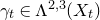 $\gamma_t \in \Lambda^{2,3}(X_t)$
solves
$\gamma_t \in \Lambda^{2,3}(X_t)$
solves
 \[E_t(\gamma_t) = \bar{\partial} \omega_t^2, \quad d \gamma_t = 0 \]
and $E_t$
is the Kodaira–Spencer operator [Reference Kodaira and SpencerKS60], which is a fourth-order elliptic operator that acts on (2,3)-forms by
$E_t$
is the Kodaira–Spencer operator [Reference Kodaira and SpencerKS60], which is a fourth-order elliptic operator that acts on (2,3)-forms by
 \[E_t = \partial \bar{\partial} \bar{\partial}^\dagger \partial^\dagger + \partial^\dagger \bar{\partial} \bar{\partial}^\dagger \partial + \partial^\dagger \partial . \]
The adjoints here are with respect to $\omega_t$
. The construction is such that
$\omega_t$
. The construction is such that $d \omega_{\mathrm{FLY},t}^2 = 0$
, and the main part of the argument in [Reference Fu, Li and YauFLY12] is to prove that
$d \omega_{\mathrm{FLY},t}^2 = 0$
, and the main part of the argument in [Reference Fu, Li and YauFLY12] is to prove that $\omega_{\mathrm{FLY},t} \gt 0$
for small enough t.
$\omega_{\mathrm{FLY},t} \gt 0$
for small enough t.
We will need the following two properties of the Fu–Li–Yau metrics. These properties can be extracted from the estimates in [Reference Fu, Li and YauFLY12], and we refer to [Reference Collins, Picard and YauCPY24] for further discussion.
-
(FLY SM I) Local model. Near each singular point
$s_i \in \mathcal{X}$
, there exist constants
$c,C,\epsilon,\delta\gt 0$
and such that for all
$t \in \Delta_\epsilon$
, we have (13)Here,
\begin{equation}\sup_{ \{ r \leq \delta \}} | g_{\mathrm{FLY},t} - c \cdot g_{\mathrm{co},t}|_{g_{\mathrm{co},t}} \leq C |t|^{{2}/{3}}.\end{equation}
$\Delta_\epsilon = \{ t \in \mathbb{C} : |t|< \epsilon \}$
.
-
(FLY SM II) Uniform convergence. For any compact set
$K \subset (X_0)_{\mathrm{reg}}$
, the sequence
$\Phi_t^* g_{\mathrm{FLY},t}$
converges uniformly to
$g_{\mathrm{FLY},0}$
as
$t \rightarrow 0$
on K.





Our main theorem on the smoothings takes the following form.
Theorem 2.11. The compact metric spaces $(X_t, d_{\mathrm{FLY},t})$
converge to
$(X_t, d_{\mathrm{FLY},t})$
converge to $(X_0,d_{\mathrm{FLY},0})$
in the Gromov–Hausdorff topology as
$(X_0,d_{\mathrm{FLY},0})$
in the Gromov–Hausdorff topology as $t \to 0$
.
$t \to 0$
.
2.4.3 Hermitian Yang–Mills metrics on the smoothing.
In order to get approximate Hermitian Yang–Mills solutions on the smoothings, Collins, Picard and Yau glued the pullback of the metric $H_0$
to the Candelas–de la Ossa metrics [Reference Collins, Picard and YauCPY24]. These approximate metrics were perturbed to obtain true solutions
$H_0$
to the Candelas–de la Ossa metrics [Reference Collins, Picard and YauCPY24]. These approximate metrics were perturbed to obtain true solutions $H_t$
to the Hermitian Yang–Mills equations. The resulting metrics
$H_t$
to the Hermitian Yang–Mills equations. The resulting metrics $H_t$
on
$H_t$
on $X_t$
solve
$X_t$
solve
 \begin{equation*} F_{H_t} \wedge \omega^2_{\mathrm{FLY},t} =0, \quad \int_{X_t} \log \frac{\det H_t}{\det g_{\mathrm{FLY},t}} \, d \textrm{vol}_{g_{\mathrm{FLY},t}} = 0.\end{equation*}
The construction of [Reference Collins, Picard and YauCPY24] is such that
 \begin{equation*}H_t = H_{t,\textrm{ref}} e^{u}, \quad | u |_{H_{t, \textrm{ref}}} + r |\nabla u|_{H_{t, \textrm{ref}}} \leq C |t|^{(1/3) |\beta|}\end{equation*}
for $|\beta| \in (0,1)$
, and
$|\beta| \in (0,1)$
, and
 \begin{equation*} H_{t,\textrm{ref}} = \chi g_{\mathrm{co},t} + (1-\chi) [(\Phi_t^{-1})^* H_0]^{1,1}\end{equation*}
and $\chi(z) = \zeta( |t|^{-\alpha} \| z \|^2 )$
for
$\chi(z) = \zeta( |t|^{-\alpha} \| z \|^2 )$
for $0<\alpha<1$
and
$0<\alpha<1$
and $\zeta: [0,\infty) \rightarrow [0,1]$
with
$\zeta: [0,\infty) \rightarrow [0,1]$
with $\zeta \equiv 1$
on [0,1] and
$\zeta \equiv 1$
on [0,1] and $\zeta \equiv 0$
on
$\zeta \equiv 0$
on $[2,\infty)$
.
$[2,\infty)$
.
The metrics $H_t$
are uniformly equivalent to
$H_t$
are uniformly equivalent to $g_{\mathrm{FLY},t}$
, so that
$g_{\mathrm{FLY},t}$
, so that
 \begin{equation} C^{-1} \cdot g_{\mathrm{FLY},t} \leq H_t \leq C \cdot g_{\mathrm{FLY},t}.\end{equation}
Furthermore, for any compact set $K \subset (X_0)_{\mathrm{reg}}$
, the sequence
$K \subset (X_0)_{\mathrm{reg}}$
, the sequence $\Phi_t^* H_t$
converges uniformly to
$\Phi_t^* H_t$
converges uniformly to $H_0$
as
$H_0$
as $t \rightarrow 0$
on K. We will show the Gromov–Hausdorff convergence of the Yang–Mills metrics.
$t \rightarrow 0$
on K. We will show the Gromov–Hausdorff convergence of the Yang–Mills metrics.
Theorem 2.12. The compact metric spaces $(X_t, d_{H_t})$
converge to
$(X_t, d_{H_t})$
converge to $(X_0, d_{H_0})$
in the Gromov–Hausdorff topology as
$(X_0, d_{H_0})$
in the Gromov–Hausdorff topology as $t \to 0$
.
$t \to 0$
.
2.5 Notation and conventions
Before we continue with our study of conifold transitions, we establish a general notational guideline due to the sheer number of metrics involved.
When working with quantities related to metrics on small resolutions ( $\widehat{X}$
and
$\widehat{X}$
and $\widehat{V}$
), we will include a hat and a subscript to denote the metric being used. We will also use the parameters a and b for families of metrics on these spaces.
$\widehat{V}$
), we will include a hat and a subscript to denote the metric being used. We will also use the parameters a and b for families of metrics on these spaces.
In a similar vein, analogous quantities on the smoothings ( $X_t$
and
$X_t$
and $V_t$
) and singular spaces (
$V_t$
) and singular spaces ( $X_0$
and
$X_0$
and $V_0$
) will not have a hat, but will include an appropriate subscript. The parameters used for families of metrics here will be s and t.
$V_0$
) will not have a hat, but will include an appropriate subscript. The parameters used for families of metrics here will be s and t.
At times, we will present lemmas and results that can be applied in more general settings encompassing both the small resolution and the smoothings. In this setting, we will not include the hat, but we will use the Greek letters $\alpha$
and
$\alpha$
and $\beta$
as parameters.
$\beta$
as parameters.
For example, see Table 1.
Notation

In addition, we adopt the convention that C denotes a generic positive constant that may change from line to line but does not depend on a or t.
3. Gromov–Hausdorff continuity in the regular case
In this section, we show Gromov–Hausdorff continuity of the geometries $(\widehat{X},\widehat{d}_{\mathrm{FLY},a})$
and
$(\widehat{X},\widehat{d}_{\mathrm{FLY},a})$
and $(\widehat{X},\widehat{d}_{\widehat{H}_a})$
for
$(\widehat{X},\widehat{d}_{\widehat{H}_a})$
for $a \gt 0$
, as well as
$a \gt 0$
, as well as $(X_t,d_{\mathrm{FLY},t})$
and
$(X_t,d_{\mathrm{FLY},t})$
and $(X_t,d_{H_t})$
for
$(X_t,d_{H_t})$
for $t \neq 0$
. That is, we show that the variations of geometry induced by a conifold transition are a continuous process in
$t \neq 0$
. That is, we show that the variations of geometry induced by a conifold transition are a continuous process in $\mathcal{M}$
away from the singular conifold. Namely, we have the following theorem.
$\mathcal{M}$
away from the singular conifold. Namely, we have the following theorem.
Theorem 3.1. The following paths $(0,1] \to \mathcal{M}$
are continuous in the Gromov–Hausdorff topology:
$(0,1] \to \mathcal{M}$
are continuous in the Gromov–Hausdorff topology:
-
(i)
$a \mapsto (\widehat{X},\widehat{d}_{\mathrm{FLY},a})$
; -
(ii)
$a \mapsto (\widehat{X},\widehat{d}_{H_a})$
.
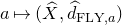
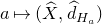
Furthermore, the following maps $\Delta_\epsilon \setminus \{0\} \to \mathcal{M}$
are continuous in the Gromov–Hausdorff topology:
$\Delta_\epsilon \setminus \{0\} \to \mathcal{M}$
are continuous in the Gromov–Hausdorff topology:
-
(iii)
$t \mapsto (X_t,d_{\mathrm{FLY},t})$
; -
(iv)
$t \mapsto (X_t,d_{H_t})$
.


Extending this continuity to the singular spaces obtained when $a=t=0$
is a more difficult task, which we will describe in §4. Our final result will be that the maps
$a=t=0$
is a more difficult task, which we will describe in §4. Our final result will be that the maps $[0,1] \rightarrow \mathcal{M}$
and
$[0,1] \rightarrow \mathcal{M}$
and $\Delta_\epsilon \rightarrow \mathcal{M}$
are continuous, but in this current section we only consider the geometries away from
$\Delta_\epsilon \rightarrow \mathcal{M}$
are continuous, but in this current section we only consider the geometries away from $X_0$
.
$X_0$
.
3.1 Gromov–Hausdorff vs. uniform convergence
Since Riemannian manifolds exhibit more structure than that of a metric space, there is considerably more flexibility when defining notions of continuity of the geometry of a family of Riemannian manifolds than that of continuity in the Gromov–Hausdorff topology. In particular, a very natural way to define continuity of the geometry is through some continuity condition on a family of metrics. As the following well-known lemma shows, the Gromov–Hausdorff topology is weaker than the topology of uniform convergence of Riemannian metrics. Many similar results can be found in the literature, cf. Example 7.4.4 of [Reference Burago, Burago and IvanovBBI01], and we include the proof as a warm-up.
Proposition 2. Let $g_\alpha$
be a family of metrics on a connected, compact manifold X of dimension n, where the parameter
$g_\alpha$
be a family of metrics on a connected, compact manifold X of dimension n, where the parameter $\alpha \in U$
lies in an open set which we take to be either real or complex:
$\alpha \in U$
lies in an open set which we take to be either real or complex: $U \subset \mathbb{R}$
or
$U \subset \mathbb{R}$
or $U \subset \mathbb{C}$
. Fixing a parameter
$U \subset \mathbb{C}$
. Fixing a parameter $\beta \in U$
, suppose that
$\beta \in U$
, suppose that $\alpha \mapsto g_{\alpha}$
is continuous at
$\alpha \mapsto g_{\alpha}$
is continuous at $\alpha = \beta$
in the
$\alpha = \beta$
in the $L^{\infty}$
norm with respect to
$L^{\infty}$
norm with respect to $g_{\beta}$
. Then
$g_{\beta}$
. Then $\alpha \mapsto (X,d_{g_{\alpha}})$
is continuous at
$\alpha \mapsto (X,d_{g_{\alpha}})$
is continuous at $\alpha=\beta$
in the Gromov–Hausdorff topology.
$\alpha=\beta$
in the Gromov–Hausdorff topology.
Remark 5. Since X is compact, all metrics on X are uniformly equivalent. That is, given two metrics $g,\tilde{g}$
on X, there is some
$g,\tilde{g}$
on X, there is some $C \gt 1$
such that
$C \gt 1$
such that
 \[ C^{-1} \cdot g \lt \tilde{g} \lt C \cdot g. \]
Thus, the continuity assumption in Proposition 2 could be replaced by continuity of the family of metrics $g_{\alpha}$
in the
$g_{\alpha}$
in the $L^{\infty}$
norm with respect to any metric on X.
$L^{\infty}$
norm with respect to any metric on X.
Proof. Let $0 \lt \epsilon \lt 1$
and fix a parameter
$0 \lt \epsilon \lt 1$
and fix a parameter $\beta$
. Consider the identity map
$\beta$
. Consider the identity map $(X,d_{g_{\alpha}}) \to (X,d_{g_{\beta}})$
. This map is surjective, so it suffices to show that it is an
$(X,d_{g_{\alpha}}) \to (X,d_{g_{\beta}})$
. This map is surjective, so it suffices to show that it is an $(C\epsilon)$
-isometry when
$(C\epsilon)$
-isometry when $|\alpha-\beta|$
is small, for some constant C independent of
$|\alpha-\beta|$
is small, for some constant C independent of $\alpha$
.
$\alpha$
.
The $L^\infty$
continuity of the metrics
$L^\infty$
continuity of the metrics $g_\alpha$
at
$g_\alpha$
at $\alpha=\beta$
implies that we may choose
$\alpha=\beta$
implies that we may choose $\delta \gt 0$
sufficiently small so that if
$\delta \gt 0$
sufficiently small so that if $|\alpha-\beta| \lt \delta$
, then
$|\alpha-\beta| \lt \delta$
, then $\sup_{X} |g_{\alpha} - g_{\beta}|_{g_{\beta}} \lt \epsilon$
. It follows that there exists some
$\sup_{X} |g_{\alpha} - g_{\beta}|_{g_{\beta}} \lt \epsilon$
. It follows that there exists some $\epsilon'=\epsilon'(\delta) \in \mathbb{R}$
such that for all
$\epsilon'=\epsilon'(\delta) \in \mathbb{R}$
such that for all $|\alpha-\beta|<\delta$
, we have
$|\alpha-\beta|<\delta$
, we have
 \begin{equation*} (1-\epsilon') \cdot g_{\beta} \leq g_{\alpha} \leq (1+\epsilon') \cdot g_{\beta}.\end{equation*}
Thus for any $\alpha$
with
$\alpha$
with $|\alpha-\beta|<\delta$
, the length of a curve
$|\alpha-\beta|<\delta$
, the length of a curve $\gamma$
satisfies
$\gamma$
satisfies $L_{\alpha}(\gamma) \leq (1+\epsilon') \cdot L_{\beta}(\gamma)$
. It follows that
$L_{\alpha}(\gamma) \leq (1+\epsilon') \cdot L_{\beta}(\gamma)$
. It follows that $D := (1+\epsilon') \cdot \text{diam}_\beta (X) \geq \text{diam}_\alpha (X)$
for all
$D := (1+\epsilon') \cdot \text{diam}_\beta (X) \geq \text{diam}_\alpha (X)$
for all $\alpha$
with
$\alpha$
with $|\alpha-\beta|<\delta$
.
$|\alpha-\beta|<\delta$
.
Pick points $p,q \in X$
and choose minimizing geodesics
$p,q \in X$
and choose minimizing geodesics $\gamma_{\alpha}, \gamma_{\beta}: [0,1] \to X$
from p to q in the
$\gamma_{\alpha}, \gamma_{\beta}: [0,1] \to X$
from p to q in the $g_\alpha$
and
$g_\alpha$
and $g_{\beta}$
metrics, respectively. We have that
$g_{\beta}$
metrics, respectively. We have that $\gamma_{\alpha}(0) = \gamma_{\beta}(0) = p$
and
$\gamma_{\alpha}(0) = \gamma_{\beta}(0) = p$
and $\gamma_{\alpha}(1) = \gamma_{\beta}(1) = q$
, and furthermore
$\gamma_{\alpha}(1) = \gamma_{\beta}(1) = q$
, and furthermore $L_{\alpha}(\gamma_{\alpha}) = d_{\alpha} (p,q)$
and
$L_{\alpha}(\gamma_{\alpha}) = d_{\alpha} (p,q)$
and $L_{\beta}(\gamma_\beta) = d_{\beta}(p,q)$
. Comparing the lengths of
$L_{\beta}(\gamma_\beta) = d_{\beta}(p,q)$
. Comparing the lengths of $\gamma_{\alpha}$
and
$\gamma_{\alpha}$
and $\gamma_{\beta}$
in the metrics
$\gamma_{\beta}$
in the metrics $g_{\alpha}$
and
$g_{\alpha}$
and $g_{\beta}$
, we note that
$g_{\beta}$
, we note that
 \begin{align*}\begin{split} |L_{\alpha}(\gamma_{\alpha}) - L_{\beta}(\gamma_{\alpha})| & \leq \int_0^1 |g_{\alpha} - g_{\beta}|_{g_{\alpha}} \cdot|\dot{\gamma_{\alpha}}|_{g_{\alpha}} \, ds \\ & \leq \Big(\sup_{X} \, |g_{\alpha} - g_{\beta}|_{g_{\alpha}} \Big) \cdot \int_0^1 |\dot{\gamma_{\alpha}}|_{g_{\alpha}}\,ds \\ & \lt D \epsilon. \end{split} \end{align*}
Similarly, we have $|L_{\alpha}(\gamma_{\beta}) - L_{\beta}(\gamma_{\beta})| \lt D \epsilon$
. Then we see that for
$|L_{\alpha}(\gamma_{\beta}) - L_{\beta}(\gamma_{\beta})| \lt D \epsilon$
. Then we see that for $|{\alpha}-{\beta}| \lt \delta$
, we have
$|{\alpha}-{\beta}| \lt \delta$
, we have
 \begin{align*} d_{\alpha}(p,q) &\leq L_{\alpha}(\gamma_{\beta}) \leq L_\beta(\gamma_\beta) + D\epsilon \\ &= d_{\beta}(p,q) + D \epsilon. \end{align*}
Similarly, $d_{\beta}(p,q) \lt d_{\alpha}(p,q) + D\epsilon$
, so that
$d_{\beta}(p,q) \lt d_{\alpha}(p,q) + D\epsilon$
, so that $|d_{\alpha}(p,q) - d_{\beta}(p,q)| \lt D\epsilon$
if
$|d_{\alpha}(p,q) - d_{\beta}(p,q)| \lt D\epsilon$
if $|{\alpha}-{\beta}| \lt \delta$
. Since this choice of
$|{\alpha}-{\beta}| \lt \delta$
. Since this choice of $\delta$
does not depend on the choice of
$\delta$
does not depend on the choice of $p,q \in X$
, the identity map is a
$p,q \in X$
, the identity map is a $D\epsilon$
-isometry, completing the proof.
$D\epsilon$
-isometry, completing the proof.
When applying this statement to the geometry of the smoothings $X_t$
, we will use the following variant.
$X_t$
, we will use the following variant.
Corollary 1. Let $\{ (X_{\alpha},g_\alpha) \}$
be a family of compact Riemannian manifolds parametrized by
$\{ (X_{\alpha},g_\alpha) \}$
be a family of compact Riemannian manifolds parametrized by $\alpha \in U \subset \mathbb{C}$
. Fix
$\alpha \in U \subset \mathbb{C}$
. Fix $\beta \in U$
, and suppose that for each
$\beta \in U$
, and suppose that for each $\alpha$
there is a diffeomorphism
$\alpha$
there is a diffeomorphism $F_\alpha: X_\beta \rightarrow X_\alpha$
. Suppose
$F_\alpha: X_\beta \rightarrow X_\alpha$
. Suppose $F_\alpha^* g_\alpha \rightarrow g_\beta$
in the
$F_\alpha^* g_\alpha \rightarrow g_\beta$
in the $L^\infty$
norm with respect to
$L^\infty$
norm with respect to $g_\beta$
as
$g_\beta$
as $\alpha \rightarrow \beta$
. Then
$\alpha \rightarrow \beta$
. Then $(X_{\alpha},d_{g_{\alpha}}) \to (X_{\beta},d_{g_{\beta}})$
in the Gromov–Hausdorff topology as
$(X_{\alpha},d_{g_{\alpha}}) \to (X_{\beta},d_{g_{\beta}})$
in the Gromov–Hausdorff topology as $\alpha \to \beta$
.
$\alpha \to \beta$
.
Proof. This follows by applying the proposition above to the family of metrics $F_\alpha^* g_{\alpha}$
on the fixed manifold
$F_\alpha^* g_{\alpha}$
on the fixed manifold $X_{\beta}$
. Thus,
$X_{\beta}$
. Thus, $(X_{\beta}, F_\alpha^* g_{\alpha}) \to (X_{\beta}, g_{\beta})$
in the Gromov–Hausdorff topology as
$(X_{\beta}, F_\alpha^* g_{\alpha}) \to (X_{\beta}, g_{\beta})$
in the Gromov–Hausdorff topology as $\alpha \to \beta$
. Since
$\alpha \to \beta$
. Since $(X_{\beta}, F_\alpha^* g_{\alpha})$
is isometric to
$(X_{\beta}, F_\alpha^* g_{\alpha})$
is isometric to $(X_{\alpha},g_{\alpha})$
, the result follows.
$(X_{\alpha},g_{\alpha})$
, the result follows.
3.2 Small-resolution metrics
$\widehat{g}_{\mathrm{FLY},a}$

In order to prove Theorem 3.1, it suffices by Proposition 2 to show that each of the families of metrics is continuous in the $L^{\infty}$
norm. To that end, we will show in this subsection that the family
$L^{\infty}$
norm. To that end, we will show in this subsection that the family $\widehat{g}_{\mathrm{FLY},a}$
is continuous in the
$\widehat{g}_{\mathrm{FLY},a}$
is continuous in the $L^{\infty}$
norm.
$L^{\infty}$
norm.
Lemma 1. The Fu–Li–Yau metrics $\{\widehat{g}_{\mathrm{FLY},a} \mid a \in (0,1]\}$
on
$\{\widehat{g}_{\mathrm{FLY},a} \mid a \in (0,1]\}$
on $\widehat{X}$
satisfy the continuity condition of Proposition 2.
$\widehat{X}$
satisfy the continuity condition of Proposition 2.
Proof. Let $b \in (0,1]$
. Recall that the Fu–Li–Yau metrics are obtained via a gluing construction which interpolates between a multiple of the Candelas–de la Ossa metrics (near the
$b \in (0,1]$
. Recall that the Fu–Li–Yau metrics are obtained via a gluing construction which interpolates between a multiple of the Candelas–de la Ossa metrics (near the $(-1,-1)$
-curves) and the ambient Calabi–Yau metric (away from the
$(-1,-1)$
-curves) and the ambient Calabi–Yau metric (away from the $(-1,-1)$
-curves) [Reference Collins, Picard and YauCPY24, Reference Fu, Li and YauFLY12]. The gluing region is independent of the parameter a, and
$(-1,-1)$
-curves) [Reference Collins, Picard and YauCPY24, Reference Fu, Li and YauFLY12]. The gluing region is independent of the parameter a, and $\widehat{\omega}_{\mathrm{FLY},a}^2 - \widehat{\omega}_{\mathrm{FLY},b}^2$
is supported on open sets around each
$\widehat{\omega}_{\mathrm{FLY},a}^2 - \widehat{\omega}_{\mathrm{FLY},b}^2$
is supported on open sets around each $(-1,-1)$
-curve, and in particular we have the following expression on the local models with
$(-1,-1)$
-curve, and in particular we have the following expression on the local models with $\| z \|^2 \lt 1$
:
$\| z \|^2 \lt 1$
:
 \begin{equation} \begin{aligned} \widehat{\omega}_{\mathrm{FLY},a}^2 - \widehat{\omega}_{\mathrm{FLY},b}^2 &= C\frac{2R^{-1}}{3} \sqrt{-1} \partial \overline{\partial} \Big( \chi \Big( \frac{2R^2}{3} f_a(\|z\|^2) \Big) (\sqrt{-1} \partial \overline{\partial} f_a (\|z\|^2) + 8a^2 \pi^* \omega_{FS}) \Big) \\[5pt] &\quad - C\frac{2R^{-1}}{3} \sqrt{-1} \partial \overline{\partial} \Big( \chi \Big( \frac{2R^2}{3} f_b(\|z\|^2) \Big) (\sqrt{-1} \partial \overline{\partial} f_b (\|z\|^2) + 8b^2 \pi^* \omega_{FS}) \Big), \end{aligned} \end{equation}
where C and R are constants, $\chi$
is a smooth function, and
$\chi$
is a smooth function, and $f_s$
are a family of smooth functions such that
$f_s$
are a family of smooth functions such that $f_s(x) = s^2 f_1 ({x}/{s^3})$
and
$f_s(x) = s^2 f_1 ({x}/{s^3})$
and
 \begin{equation*} (x f_1')^3 + 6(x f_1')^2 = x^2 \end{equation*}
(see [Reference Collins, Picard and YauCPY24]). It follows that the function $|\widehat{\omega}_{\mathrm{FLY},a}^2 - \widehat{\omega}_{\mathrm{FLY},b}^2|^2_{g_{\mathrm{FLY},b}}$
is smooth in a and p.
$|\widehat{\omega}_{\mathrm{FLY},a}^2 - \widehat{\omega}_{\mathrm{FLY},b}^2|^2_{g_{\mathrm{FLY},b}}$
is smooth in a and p.
Since $b \neq 0$
, we can pick some
$b \neq 0$
, we can pick some $h \gt 0$
such that
$h \gt 0$
such that $I = [b-h,b+h] \subset (0,1]$
(or
$I = [b-h,b+h] \subset (0,1]$
(or $I = [1-h,1] \subseteq (0,1]$
in the case where
$I = [1-h,1] \subseteq (0,1]$
in the case where $b = 1)$
. One can check that in coordinates around a point
$b = 1)$
. One can check that in coordinates around a point $p \in \widehat{X}$
, each component in (15) is smooth in a and p. In particular, differentiating the function
$p \in \widehat{X}$
, each component in (15) is smooth in a and p. In particular, differentiating the function $f_a (\|z\|^2)$
involves uniform bounds since we have the expression
$f_a (\|z\|^2)$
involves uniform bounds since we have the expression $f_a(\|z\|^2) = a^2 f_1 ({\|z\|^2}/{a^3})$
and also because
$f_a(\|z\|^2) = a^2 f_1 ({\|z\|^2}/{a^3})$
and also because $a \gt 0$
in our interval so that
$a \gt 0$
in our interval so that ${\|z\|^2}/{a^3}$
lies in a compact set.
${\|z\|^2}/{a^3}$
lies in a compact set.
It follows that the covariant derivative of $|\widehat{\omega}_{\mathrm{FLY},a}^2 - \widehat{\omega}_{\mathrm{FLY},b}^2|^2_{g_{\mathrm{FLY},b}}$
is continuous on
$|\widehat{\omega}_{\mathrm{FLY},a}^2 - \widehat{\omega}_{\mathrm{FLY},b}^2|^2_{g_{\mathrm{FLY},b}}$
is continuous on $I \times \widehat{X}$
. By compactness, we obtain uniform boundedness of the covariant derivative on I. By a corollary of the Arzelà–Ascoli theorem, the pointwise convergence of the function
$I \times \widehat{X}$
. By compactness, we obtain uniform boundedness of the covariant derivative on I. By a corollary of the Arzelà–Ascoli theorem, the pointwise convergence of the function $|\widehat{\omega}_{\mathrm{FLY},a}^2 - \widehat{\omega}_{\mathrm{FLY},b}^2|^2_{g_{\mathrm{FLY},b}}$
is actually uniform.
$|\widehat{\omega}_{\mathrm{FLY},a}^2 - \widehat{\omega}_{\mathrm{FLY},b}^2|^2_{g_{\mathrm{FLY},b}}$
is actually uniform.
A positive $(n-1,n-1)$
-form has a unique
$(n-1,n-1)$
-form has a unique $(n-1)$
th root and this is determined in a continuous fashion (see e.g. [Reference MichelsohnMic82]). It follows that
$(n-1)$
th root and this is determined in a continuous fashion (see e.g. [Reference MichelsohnMic82]). It follows that $\sup |\widehat{g}_{\mathrm{co},a} - \widehat{g}_{\mathrm{co},b}|_{\widehat{g}_{\mathrm{co},b}}$
approaches 0 as
$\sup |\widehat{g}_{\mathrm{co},a} - \widehat{g}_{\mathrm{co},b}|_{\widehat{g}_{\mathrm{co},b}}$
approaches 0 as $a \rightarrow b$
.
$a \rightarrow b$
.
We can now apply Proposition 2 to this path of spaces to obtain the desired Gromov–Hausdorff continuity.
3.3 Smoothing metrics
$g_{\mathrm{FLY},t}$

We prove the analogous results of §3.2 for the smoothings.
Let $\mu: \mathcal{X} \rightarrow \Delta$
be a holomorphic smoothing of
$\mu: \mathcal{X} \rightarrow \Delta$
be a holomorphic smoothing of $X_0$
and let
$X_0$
and let $X_t = \mu^{-1}(t)$
. Fix
$X_t = \mu^{-1}(t)$
. Fix $s \neq 0$
and consider the smoothings
$s \neq 0$
and consider the smoothings $X_t$
nearby
$X_t$
nearby $X_s$
. As this is a smooth family of complex manifolds, by Ehresmann’s lemma there exists a smoothly varying family of diffeomorphisms
$X_s$
. As this is a smooth family of complex manifolds, by Ehresmann’s lemma there exists a smoothly varying family of diffeomorphisms $F_t: X_s \rightarrow X_t$
such that
$F_t: X_s \rightarrow X_t$
such that $F_s$
is the identity map.
$F_s$
is the identity map.
Recall that the Fu–Li–Yau metrics [Reference Fu, Li and YauFLY12] on the smoothings are obtained by: (1) pullback and a gluing construction leading to a pre-perturbed metric $g_t$
; followed by (2) a perturbation to a balanced metric
$g_t$
; followed by (2) a perturbation to a balanced metric $g_{\mathrm{FLY},t}$
.
$g_{\mathrm{FLY},t}$
.
We see that the expression (11) for $\omega^2_t$
is smooth in the parameter t and can employ the method in the proof of Lemma 1. The metric
$\omega^2_t$
is smooth in the parameter t and can employ the method in the proof of Lemma 1. The metric $g_t$
on
$g_t$
on $X_t$
is extracted from
$X_t$
is extracted from $\omega_t$
via a square-root construction (see e.g. [Reference MichelsohnMic82]), and since the dependence on t is explicit here and
$\omega_t$
via a square-root construction (see e.g. [Reference MichelsohnMic82]), and since the dependence on t is explicit here and $F_t: X_s \rightarrow X_t$
varies smoothly with
$F_t: X_s \rightarrow X_t$
varies smoothly with $F_s=\text{{id}}$
, we can see that
$F_s=\text{{id}}$
, we can see that
 \[\lim_{t \rightarrow s} \sup_{X_s} | F_t^* g_t - g_s |_{g_s} = 0. \]
Corollary 1 applies to $(X_t,g_t)$
; however, these are not the Fu–Li–Yau metrics as these do not satisfy
$(X_t,g_t)$
; however, these are not the Fu–Li–Yau metrics as these do not satisfy $d \omega_t^2=0$
. For this we need to estimate the correction term
$d \omega_t^2=0$
. For this we need to estimate the correction term $\gamma_t$
appearing in (12). As this term
$\gamma_t$
appearing in (12). As this term $\gamma_t$
comes from solving
$\gamma_t$
comes from solving $E_t(\gamma_t) = \bar{\partial} \omega_t^2$
, we need to deduce from the fact that the right-hand sides
$E_t(\gamma_t) = \bar{\partial} \omega_t^2$
, we need to deduce from the fact that the right-hand sides $\bar{\partial} \omega_t^2$
vary smoothly for
$\bar{\partial} \omega_t^2$
vary smoothly for $t \neq 0$
that the solutions
$t \neq 0$
that the solutions $\gamma_t$
vary smoothly. We first need to study some properties of the Kodaira–Spencer operator
$\gamma_t$
vary smoothly. We first need to study some properties of the Kodaira–Spencer operator $E_t$
(which, in this case, is determined with respect to the auxiliary metric
$E_t$
(which, in this case, is determined with respect to the auxiliary metric $\omega_t$
).
$\omega_t$
).
Lemma 2. Let $\widehat{X} \rightarrow X_0 \rightsquigarrow X_t$
be a conifold transition from an initial Kähler Calabi–Yau threefold with finite fundamental group. Endow
$\widehat{X} \rightarrow X_0 \rightsquigarrow X_t$
be a conifold transition from an initial Kähler Calabi–Yau threefold with finite fundamental group. Endow $X_t$
with the auxiliary Hermitian metric
$X_t$
with the auxiliary Hermitian metric $\omega_t$
from the Fu–Li–Yau construction. Then
$\omega_t$
from the Fu–Li–Yau construction. Then $E_t: \Lambda^{2,3}(X_t) \rightarrow \Lambda^{2,3}(X_t)$
satisfies
$E_t: \Lambda^{2,3}(X_t) \rightarrow \Lambda^{2,3}(X_t)$
satisfies $\text{ ker}\,E_t = \{ 0 \}$
for all
$\text{ ker}\,E_t = \{ 0 \}$
for all $0<|t| \ll 1$
.
$0<|t| \ll 1$
.
Proof. Let $\chi \in \Lambda^{2,3}(X_t)$
be such that
$\chi \in \Lambda^{2,3}(X_t)$
be such that $\chi \in \text{ker}\,E_t$
. Integrating by parts over the identity
$\chi \in \text{ker}\,E_t$
. Integrating by parts over the identity $\langle E_t \chi, \chi \rangle = 0$
implies
$\langle E_t \chi, \chi \rangle = 0$
implies
 \[\partial \chi = 0, \quad \bar{\partial}^\dagger \partial^\dagger \chi = 0. \]
Next, we note that $\partial^\dagger \chi \in \Lambda^{1,3}(X_t)$
and so
$\partial^\dagger \chi \in \Lambda^{1,3}(X_t)$
and so $\bar{\partial} (\partial^\dagger \chi) = 0$
by type consideration. It is noticed in [Reference Fu, Li and YauFLY12] that
$\bar{\partial} (\partial^\dagger \chi) = 0$
by type consideration. It is noticed in [Reference Fu, Li and YauFLY12] that
 \[H^{1,3}(X_t,\mathbb{C}) = H^0(X_t,T X_t) = 0 \]
by using $H^{1,3}(\widehat{X},\mathbb{C})=0$
on the small resolution together with Hartogs’ lemma; we refer to [Reference Fu, Li and YauFLY12] for the proof. Therefore,
$H^{1,3}(\widehat{X},\mathbb{C})=0$
on the small resolution together with Hartogs’ lemma; we refer to [Reference Fu, Li and YauFLY12] for the proof. Therefore,
 \[\partial^\dagger \chi = \bar{\partial} \beta \]
and so
 \[\langle \partial^\dagger \chi, \partial^\dagger \chi \rangle = \langle \bar{\partial}^\dagger \partial^\dagger \chi, \beta \rangle= 0. \]
We conclude that if $\chi \in \Lambda^{2,3} \cap \text{ker}\,E_t$
, then
$\chi \in \Lambda^{2,3} \cap \text{ker}\,E_t$
, then $\partial \chi = \partial^\dagger \chi = 0$
. It follows that
$\partial \chi = \partial^\dagger \chi = 0$
. It follows that $\psi = \bar{\chi} \in \Lambda^{3,2}(X_t)$
solves
$\psi = \bar{\chi} \in \Lambda^{3,2}(X_t)$
solves
 \[\Delta_{\bar{\partial}} \psi = 0, \quad \Delta_{\bar{\partial}} = \bar{\partial} \bar{\partial}^\dagger + \bar{\partial}^\dagger \bar{\partial}. \]
By the Hodge theorem, this defines an element in Dolbeault cohomology, and since $X_t$
has trivial canonical bundle, then
$X_t$
has trivial canonical bundle, then $H^{3,2}(X_t,\mathbb{C}) = H^2(X_t,\Omega^3_{X_t}) = H^2(X_t,\mathcal{O}_{X_t})$
. Lemma 8.2 in [Reference FriedmanFri91] states that if
$H^{3,2}(X_t,\mathbb{C}) = H^2(X_t,\Omega^3_{X_t}) = H^2(X_t,\mathcal{O}_{X_t})$
. Lemma 8.2 in [Reference FriedmanFri91] states that if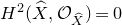 $H^2(\widehat{X},\mathcal{O}_{\widehat{X}}) = 0$
, then
$H^2(\widehat{X},\mathcal{O}_{\widehat{X}}) = 0$
, then $H^2(X_t,\mathcal{O}_{X_t}) =0$
. Since
$H^2(X_t,\mathcal{O}_{X_t}) =0$
. Since
 \[H^2(\widehat{X},\mathcal{O}_{\widehat{X}}) = H^{0,2}(\widehat{X},\mathbb{C})= H^{0,1}(\widehat{X},\mathbb{C})= 0 \]
on the initial Kähler Calabi–Yau threefold with finite fundamental group, we conclude that $H^{3,2}(X_t,\mathbb{C}) =0$
and so
$H^{3,2}(X_t,\mathbb{C}) =0$
and so $\psi = 0$
.
$\psi = 0$
.
We will also need some uniform estimates as $t \rightarrow s$
. This is a standard argument given that the kernel of E is trivial and
$t \rightarrow s$
. This is a standard argument given that the kernel of E is trivial and $X_s$
is smooth.
$X_s$
is smooth.
Lemma 3. Fix $s\gt 0$
. There exists
$s\gt 0$
. There exists $\epsilon\gt 0$
and
$\epsilon\gt 0$
and $C\gt 1$
such that
$C\gt 1$
such that
 \begin{equation} \| \gamma_t \|_{C^{4,\alpha}(X_t)} \leq C \| E_t (\gamma_t) \|_{C^\alpha(X_t)}\end{equation}
for all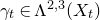 $\gamma_t \in \Lambda^{2,3}(X_t)$
with
$\gamma_t \in \Lambda^{2,3}(X_t)$
with $|t-s|<\epsilon$
. Here, each norm on
$|t-s|<\epsilon$
. Here, each norm on $X_t$
is taken with respect to the auxiliary Hermitian metrics
$X_t$
is taken with respect to the auxiliary Hermitian metrics $\omega_t$
from the Fu–Li–Yau construction.
$\omega_t$
from the Fu–Li–Yau construction.
Proof. Since the compact manifolds $X_t$
deform smoothly to the compact manifold
$X_t$
deform smoothly to the compact manifold $X_s$
, the Schauder estimates
$X_s$
, the Schauder estimates
 \begin{equation} \| \gamma_t \|_{C^{4,\alpha}(X_t)} \leq C (\| \gamma_t \|_{C^0(X_t)} + \| E_t (\gamma_t) \|_{C^\alpha(X_t)} )\end{equation}
hold uniformly for all t close to s, where the norms on $X_t$
are taken with respect to
$X_t$
are taken with respect to $\omega_t$
. We would like to upgrade this estimate to (16).
$\omega_t$
. We would like to upgrade this estimate to (16).
Suppose (16) is false, so that there exists a sequence $t_i \rightarrow s$
and constants
$t_i \rightarrow s$
and constants $C_i \rightarrow \infty$
with
$C_i \rightarrow \infty$
with
 \[\| \gamma_{t_i} \|_{C^{4,\alpha}(X_{t_i})} \geq C_i \| E_{t_i} (\gamma_{t_i}) \|_{C^\alpha(X_{t_i})}. \]
Consider $\tilde{\gamma}_i = \gamma_{t_i} / \| \gamma_{t_i} \|_{C^{4,\alpha}(X_{t_i})}$
. As
$\tilde{\gamma}_i = \gamma_{t_i} / \| \gamma_{t_i} \|_{C^{4,\alpha}(X_{t_i})}$
. As
 \[\| \tilde{\gamma}_i \|_{C^{4,\alpha}(X_{t_i})} = 1, \quad \| E_{t_i} (\tilde{\gamma}_i) \|_{C^\alpha(X_{t_i})} \leq C_i^{-1}, \]
we may apply the Arzelà–Ascoli theorem to extract a convergent subsequence to a limit $\gamma_\infty$
solving
$\gamma_\infty$
solving
 \[E_s(\gamma_\infty)=0. \]
By the previous lemma, $\gamma_\infty = 0$
. This contradicts estimate (17), which implies
$\gamma_\infty = 0$
. This contradicts estimate (17), which implies
 \[1 \leq C (\| \tilde{\gamma}_i \|_{C^0(X_{t_i})} + \| E_t (\tilde{\gamma}_i) \|_{C^\alpha(X_{t_i})} ) \]
and so ${1}/{2C} \leq \| \tilde{\gamma}_i \|_{C^0(X_{t_i})}$
for all
${1}/{2C} \leq \| \tilde{\gamma}_i \|_{C^0(X_{t_i})}$
for all $t_i$
close to s, and thus
$t_i$
close to s, and thus $\| \gamma_\infty \|_{C^0(X_s)} \gt 0$
.
$\| \gamma_\infty \|_{C^0(X_s)} \gt 0$
.
Returning to the construction of the metrics $\omega_{\mathrm{FLY},t}$
, we claim
$\omega_{\mathrm{FLY},t}$
, we claim $F_t^* \gamma_t \rightarrow \gamma_s$
in
$F_t^* \gamma_t \rightarrow \gamma_s$
in $C^4(X_s)$
as
$C^4(X_s)$
as $t \rightarrow s$
. Suppose not, so that there exists
$t \rightarrow s$
. Suppose not, so that there exists $\epsilon\gt 0$
with
$\epsilon\gt 0$
with
 \begin{equation} \| F_t^* \gamma_t - \gamma_s \|_{C^4(X_s)} \geq \epsilon\end{equation}
along a subsequence $t_i \rightarrow s$
. The uniform elliptic estimate (16) implies
$t_i \rightarrow s$
. The uniform elliptic estimate (16) implies $\| \gamma_t \|_{C^{4,\alpha}(X_t)} \leq C$
, and so
$\| \gamma_t \|_{C^{4,\alpha}(X_t)} \leq C$
, and so $F_t^* \gamma_t$
is also bounded on
$F_t^* \gamma_t$
is also bounded on $(X_s,g_s)$
. Applying the Arzelà–Ascoli theorem, there is a subsequence converging to a limit
$(X_s,g_s)$
. Applying the Arzelà–Ascoli theorem, there is a subsequence converging to a limit $\gamma_\infty$
on
$\gamma_\infty$
on $X_s$
solving
$X_s$
solving
 \[E_s(\gamma_\infty) = \bar{\partial} \omega_s^2. \]
It follows that
 \[E_s (\gamma_\infty-\gamma_s) = 0 \]
and, since $\text{ker}\,E_s = \{ 0 \}$
, we conclude
$\text{ker}\,E_s = \{ 0 \}$
, we conclude $\gamma_\infty = \gamma_s$
, which contradicts (18).
$\gamma_\infty = \gamma_s$
, which contradicts (18).
Using that $F_t^* \gamma_t \rightarrow \gamma_s$
, taking a square root of (12) gives a family of metrics
$F_t^* \gamma_t \rightarrow \gamma_s$
, taking a square root of (12) gives a family of metrics $\omega_{\mathrm{FLY},t}$
varying continuously as
$\omega_{\mathrm{FLY},t}$
varying continuously as $t \rightarrow s$
, and so
$t \rightarrow s$
, and so
 \[\lim_{t \rightarrow s} \sup_{X_s} | F_t^* g_{\mathrm{FLY},t} - g_{\mathrm{FLY},s} |_{g_s} = 0. \]
By Remark 5, this convergence also holds with respect to the Fu–Li–Yau metrics $g_{\mathrm{FLY},s}$
, and thus Corollary 1 applies to
$g_{\mathrm{FLY},s}$
, and thus Corollary 1 applies to $(X_t,g_{\mathrm{FLY},t})$
. This proves that
$(X_t,g_{\mathrm{FLY},t})$
. This proves that $(X_t,d_{\mathrm{FLY},t}) \rightarrow (X_s,d_{\mathrm{FLY},s})$
in the Gromov–Hausdorff sense as
$(X_t,d_{\mathrm{FLY},t}) \rightarrow (X_s,d_{\mathrm{FLY},s})$
in the Gromov–Hausdorff sense as $t \rightarrow s$
.
$t \rightarrow s$
.
3.4 Small-resolution metrics
$\widehat{H}_a$

We return to the small resolution $\widehat{X} \rightarrow X_0$
, where there is a family of metrics
$\widehat{X} \rightarrow X_0$
, where there is a family of metrics $\widehat{H}_a$
satisfying the Hermitian Yang–Mills equation
$\widehat{H}_a$
satisfying the Hermitian Yang–Mills equation
 \[F_{\widehat{H}_a} \wedge \widehat{\omega}_{\mathrm{FLY},a}^2 = 0. \]
We will show that for $b\gt 0$
fixed,
$b\gt 0$
fixed,
 \begin{equation} \lim_{a \rightarrow b} \sup_{\widehat{X}} \| \widehat{H}_a - \widehat{H}_b \|_{\widehat{H}_b} \rightarrow 0.\end{equation}
Suppose this is false. Then there exists $\epsilon\gt 0$
and a sequence
$\epsilon\gt 0$
and a sequence $a_i \rightarrow b$
such that
$a_i \rightarrow b$
such that
 \begin{equation*}\| \widehat{H}_{a_i} - \widehat{H}_b \|_{\widehat{H}_b} \geq \epsilon, \quad \sqrt{-1} \Lambda_{\widehat{\omega}_{\mathrm{FLY},a_i}} F_{\widehat{H}_{a_i}} = 0\end{equation*}
for all $a_i$
. By the estimates in Proposition 1, we have
$a_i$
. By the estimates in Proposition 1, we have
 \begin{equation*} C^{-1} \cdot \widehat{g}_{\mathrm{FLY}, b} \leq \widehat{H}_a \leq C \cdot \widehat{g}_{\mathrm{FLY},b}.\end{equation*}
Standard estimates for the Hermitian Yang–Mills equations then give
 \begin{equation} |\nabla \widehat{H}_a|_{\widehat{g}_b} + |\nabla^2 \widehat{H}_a|_{\widehat{g}_b} \leq C.\end{equation}
For a proof of these standard estimates, see e.g. Proposition 3.9 with $r \equiv 1$
in [Reference Collins, Gukov, Picard and YauCGP+23] and the higher-order estimates which follow after, or in the Kähler case Appendix C of [Reference Jacob and WalpuskiJW18]. By the Arzelà–Ascoli theorem, we may extract a subsequence
$r \equiv 1$
in [Reference Collins, Gukov, Picard and YauCGP+23] and the higher-order estimates which follow after, or in the Kähler case Appendix C of [Reference Jacob and WalpuskiJW18]. By the Arzelà–Ascoli theorem, we may extract a subsequence $\widehat{H}_{a_{i_k}}$
converging to a limit
$\widehat{H}_{a_{i_k}}$
converging to a limit $H_\infty$
such that
$H_\infty$
such that
 \begin{equation} \| H_{\infty} - \widehat{H}_b \|_{\widehat{H}_b} \geq \epsilon, \quad \sqrt{-1} \Lambda_{\widehat{\omega}_{\mathrm{FLY},b}} F_{H_\infty} = 0.\end{equation}
This uses that $\widehat{\omega}_{\mathrm{FLY}, a_{i_k}} \rightarrow \widehat{\omega}_{\mathrm{FLY},b}$
as
$\widehat{\omega}_{\mathrm{FLY}, a_{i_k}} \rightarrow \widehat{\omega}_{\mathrm{FLY},b}$
as $a_{i_k} \rightarrow b$
, which holds by properties of the Fu–Li–Yau metrics. We now have two Hermitian Yang–Mills metrics
$a_{i_k} \rightarrow b$
, which holds by properties of the Fu–Li–Yau metrics. We now have two Hermitian Yang–Mills metrics $H_\infty$
and
$H_\infty$
and $\widehat{H}_b$
with respect to
$\widehat{H}_b$
with respect to $\widehat{\omega}_{\mathrm{FLY}, b}$
. Consider
$\widehat{\omega}_{\mathrm{FLY}, b}$
. Consider $H_\infty= e^u \widehat{H}_b$
. A classic calculation (see e.g. [Reference Uhlenbeck and YauUY86], or (A.11) below) implies
$H_\infty= e^u \widehat{H}_b$
. A classic calculation (see e.g. [Reference Uhlenbeck and YauUY86], or (A.11) below) implies
 \begin{equation} \Delta_{\widehat{\omega}_{\mathrm{FLY}, b}} |u|^2_{\widehat{H}_b} \geq C^{-1} |\bar{\partial} u|^2_{\widehat{\omega}_{\mathrm{FLY}, b},\widehat{H}_b}.\end{equation}
It follows by the maximum principle that $\bar{\partial} u = 0$
and hence u is a holomorphic endomorphism of
$\bar{\partial} u = 0$
and hence u is a holomorphic endomorphism of $T^{1,0} \widehat{X}$
. It is a well-known corollary of Yau’s theorem [Reference YauYau78] that, on a Calabi–Yau threefold
$T^{1,0} \widehat{X}$
. It is a well-known corollary of Yau’s theorem [Reference YauYau78] that, on a Calabi–Yau threefold $\widehat{X}$
with finite fundamental group, it holds that
$\widehat{X}$
with finite fundamental group, it holds that
 \begin{equation} H^0(\widehat{X},\textrm{End} \, T^{1,0} \widehat{X}) = \{ c \, \textrm{id} : c \in \mathbb{C} \}.\end{equation}
Therefore, $H_\infty = \lambda H_b$
. By the normalization condition (8), it follows that
$H_\infty = \lambda H_b$
. By the normalization condition (8), it follows that $\lambda=1$
. This contradicts (21), and thus (19) is proved, and we conclude that
$\lambda=1$
. This contradicts (21), and thus (19) is proved, and we conclude that $(\widehat{X},\widehat{d}_{\widehat{H}_a}) \rightarrow (\widehat{X},\widehat{d}_{\widehat{H}_b})$
in the Gromov–Hausdorff sense as
$(\widehat{X},\widehat{d}_{\widehat{H}_a}) \rightarrow (\widehat{X},\widehat{d}_{\widehat{H}_b})$
in the Gromov–Hausdorff sense as $a \rightarrow b$
.
$a \rightarrow b$
.
Here is one way to see (23). By Yau’s theorem, $\widehat{X}$
admits a Kähler Ricci-flat metric. A holomorphic endomorphism of
$\widehat{X}$
admits a Kähler Ricci-flat metric. A holomorphic endomorphism of $T^{1,0} \widehat{X}$
is parallel with respect to the Levi-Civita connection by a Bochner argument. This parallel endomorphism defines a
$T^{1,0} \widehat{X}$
is parallel with respect to the Levi-Civita connection by a Bochner argument. This parallel endomorphism defines a $\textrm{Hol}_p$
-linear map on
$\textrm{Hol}_p$
-linear map on $T_p \widehat{X}$
, and hence by Schur’s lemma must be a scalar multiple of the identity at each point
$T_p \widehat{X}$
, and hence by Schur’s lemma must be a scalar multiple of the identity at each point $p \in \widehat{X}$
; this scalar factor is the same at all points by holomorphy. Here we used that the restricted holonomy group
$p \in \widehat{X}$
; this scalar factor is the same at all points by holomorphy. Here we used that the restricted holonomy group $\textrm{Hol}_p = \mathrm{SU}(3)$
and acts irreducibly on
$\textrm{Hol}_p = \mathrm{SU}(3)$
and acts irreducibly on $T_p \widehat{X}$
, since
$T_p \widehat{X}$
, since $\widehat{X}$
has finite fundamental group by the de Rham splitting theorem.
$\widehat{X}$
has finite fundamental group by the de Rham splitting theorem.
3.5 Smoothing metrics
$H_t$

Fix $s \neq 0$
and consider the smoothings
$s \neq 0$
and consider the smoothings $X_t$
near the smooth fiber
$X_t$
near the smooth fiber $X_s$
with smoothly varying family of diffeomorphisms
$X_s$
with smoothly varying family of diffeomorphisms $F_t: X_s\rightarrow X_t$
, with
$F_t: X_s\rightarrow X_t$
, with $F_s$
the identity. The metrics
$F_s$
the identity. The metrics $H_t$
also satisfy continuity of the form
$H_t$
also satisfy continuity of the form
 \begin{equation} \lim_{t \rightarrow s} \| F_t^* H_t - H_s \|_{H_s} =0.\end{equation}
The proof is similar to the arguments given before: suppose $F_t^* H_t$
does not converge to
$F_t^* H_t$
does not converge to $H_s$
as
$H_s$
as $t \rightarrow s$
and extract a converging subsequence via the estimates (14) and (20). The limit solves the Hermitian Yang–Mills equation, and by uniqueness and normalization this limit must be
$t \rightarrow s$
and extract a converging subsequence via the estimates (14) and (20). The limit solves the Hermitian Yang–Mills equation, and by uniqueness and normalization this limit must be $H_s$
, which is a contradiction.
$H_s$
, which is a contradiction.
The main difference compared to the argument given in (22) is the step which establishes
 \begin{equation} H^0(X_t,\textrm{End} \, T^{1,0} X_t) = \{ c \, \textrm{id} : c \in \mathbb{C} \},\end{equation}
for all t small enough. This follows from a well-known argument as soon as we show that $T^{1,0} X_t$
is a stable bundle: stable vector bundles are simple. Since we know that
$T^{1,0} X_t$
is a stable bundle: stable vector bundles are simple. Since we know that $T^{1,0} X_t$
admits a Hermitian Yang–Mills metric, this bundle is polystable, and hence it remains to show that it cannot split holomorphically as
$T^{1,0} X_t$
admits a Hermitian Yang–Mills metric, this bundle is polystable, and hence it remains to show that it cannot split holomorphically as $T^{1,0} X_t=A_t \oplus B_t$
. Suppose, by contradiction, that there exists a sequence
$T^{1,0} X_t=A_t \oplus B_t$
. Suppose, by contradiction, that there exists a sequence $t_i \rightarrow 0$
such that the tangent bundle splits, and after a subsequence and relabeling we may assume
$t_i \rightarrow 0$
such that the tangent bundle splits, and after a subsequence and relabeling we may assume $\textrm{rk} A_{t_i} = 1$
. Define from such data a sequence of holomorphic endomorphisms
$\textrm{rk} A_{t_i} = 1$
. Define from such data a sequence of holomorphic endomorphisms $h_i \in H^0(X_{t_i}, \textrm{End} \, T^{1,0} X_{t_i})$
by
$h_i \in H^0(X_{t_i}, \textrm{End} \, T^{1,0} X_{t_i})$
by
 \[h_{t_i} =\begin{cases} \mathrm{id} & \text{on } A_{t_i}, \\[4pt] 0 & \text{on } B_{t_i}.\end{cases} \]
By compactness of holomorphic functions, on compact sets away from the singular set we may take a subsequential limit uniformly. By an exhaustion argument, a subsequence of the $t_i$
converges to a limiting endomorphism
$t_i$
converges to a limiting endomorphism
 \[h_\infty \in H^0(X_{0,\textrm{reg}}, \textrm{End} \, T^{1,0} X_{0, \textrm{reg}}). \]
Taking pointwise limits of $\mathrm{Tr} \, h_{t_i}$
and
$\mathrm{Tr} \, h_{t_i}$
and $\det \, h_{t_i}$
gives
$\det \, h_{t_i}$
gives
 \begin{equation} \mathrm{Tr} \, h_\infty = 1, \quad \det h_\infty = 0.\end{equation}
This defines a holomorphic endomorphism of the tangent bundle on $\widehat{X} \setminus E$
, and by Hartogs’ theorem this endomorphism extends to
$\widehat{X} \setminus E$
, and by Hartogs’ theorem this endomorphism extends to
 \[h_\infty \in H^0 (\widehat{X}, \textrm{End} \, T^{1,0} \widehat{X}). \]
We conclude by (23) that $h_\infty = \lambda \textrm{id}$
, which contradicts (26).
$h_\infty = \lambda \textrm{id}$
, which contradicts (26).
4. Gromov–Hausdorff convergence in the singular case
In this section, we extend Theorem 3.1 and show that conifold transitions with the Fu–Li–Yau metrics and the Hermitian Yang–Mills metrics are continuous in the Gromov–Hausdorff topology through the singular conifold at $t=a=0$
. That is, we show the following.
$t=a=0$
. That is, we show the following.
Theorem 4.1. The following four convergences hold in the Gromov–Hausdorff topology:

Therefore, the maps $[0,1] \to \mathcal{M}$
given by
$[0,1] \to \mathcal{M}$
given by
-
(i)
$a \mapsto (\widehat{X},\widehat{d}_{\mathrm{FLY},a})$
; -
(ii)
$a \mapsto (\widehat{X},\widehat{d}_{H_a})$
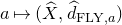
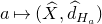
and the maps $\Delta_\epsilon \to \mathcal{M}$
given by
$\Delta_\epsilon \to \mathcal{M}$
given by
-
(iii)
$t \mapsto (X_t,d_{\mathrm{FLY},t})$
; -
(iv)
$t \mapsto (X_t,d_{H_t})$


are continuous and agree at $a=t=0$
.
$a=t=0$
.
Before starting the proofs, we discuss how to interpret the limiting spaces $(X_0,d_{\mathrm{FLY},0})$
and
$(X_0,d_{\mathrm{FLY},0})$
and $(X_0,d_{H_0})$
.
$(X_0,d_{H_0})$
.
A length structure on a topological space X consists of a class A of curves in X, and a length function $L:A \to [0,\infty)$
. The curves in A are called admissible curves. Both A and L have to satisfy a number of very natural conditions (see Definition 2.1.1 of [Reference Burago, Burago and IvanovBBI01]). The length structure determines a distance function d on X so that for all
$L:A \to [0,\infty)$
. The curves in A are called admissible curves. Both A and L have to satisfy a number of very natural conditions (see Definition 2.1.1 of [Reference Burago, Burago and IvanovBBI01]). The length structure determines a distance function d on X so that for all $p,q \in X$
, the distance d(p,q) is the infimum of the lengths of all admissible curves from p to q. A length space is a topological space X together with a length structure on X.
$p,q \in X$
, the distance d(p,q) is the infimum of the lengths of all admissible curves from p to q. A length space is a topological space X together with a length structure on X.
Remark 6. The spaces that we consider in this paper are all smooth Riemannian manifolds, with the exception of the cone $(V_0,g_{\mathrm{co},0})$
and the conifold
$(V_0,g_{\mathrm{co},0})$
and the conifold $(X_0,g_{\mathrm{FLY},0})$
or
$(X_0,g_{\mathrm{FLY},0})$
or $(X_0,H_0)$
, where there are isolated singular points. Thus, on each space considered, there is a natural length structure whose admissible curves are the piecewise differentiable curves, and whose length function is the standard Riemannian length; that is, the integral of the speed of the curve with respect to the metric. The metric is defined everywhere except at the isolated singular points, so the Riemannian length is well-defined.
$(X_0,H_0)$
, where there are isolated singular points. Thus, on each space considered, there is a natural length structure whose admissible curves are the piecewise differentiable curves, and whose length function is the standard Riemannian length; that is, the integral of the speed of the curve with respect to the metric. The metric is defined everywhere except at the isolated singular points, so the Riemannian length is well-defined.
We will make use of the following theorem (Theorem 2.5.23 of [Reference Burago, Burago and IvanovBBI01]).
Theorem 4.2. Let X be a complete, locally compact length space. Then, given any $p,q \in X$
, there exists an admissible curve
$p,q \in X$
, there exists an admissible curve $\gamma: [0,1] \to X$
such that
$\gamma: [0,1] \to X$
such that $\gamma(0)=p$
and
$\gamma(0)=p$
and $\gamma(1)=q$
, with
$\gamma(1)=q$
, with $L(\gamma)=d(p,q)$
.
$L(\gamma)=d(p,q)$
.
Lastly, we adopt the convention that the diameter of a set Q is understood to mean the intrinsic diameter, as we explain in the following definition.
Definition 4.3. Let Q be a bounded, path-connected set in a length space X. Given two points $p,q \in Q$
, the intrinsic distance from p to q is defined as
$p,q \in Q$
, the intrinsic distance from p to q is defined as $d_{\mathrm{int}}(p,q) := \inf L(\gamma)$
, where the infimum is taken over all admissible curves
$d_{\mathrm{int}}(p,q) := \inf L(\gamma)$
, where the infimum is taken over all admissible curves $\gamma$
from p to q contained in Q. The diameter of Q is defined by
$\gamma$
from p to q contained in Q. The diameter of Q is defined by
 \[\text{diam}(Q) := \sup\limits_{p,q \in Q} d_{\mathrm{int}}(p,q). \]
Note that this is a non-standard definition of diameter, since many authors take the diameter of Q to be the supremum of the distance (in X) between pairs of points in Q.
4.1 Reduction of a curve
In order to prove our main lemma (Lemma 5), we first need the following curve-reduction lemma.
Lemma 4. Suppose $Q_1, \ldots, Q_k$
are disjoint, closed, path-connected, bounded sets in a complete, locally compact length space X, and let
$Q_1, \ldots, Q_k$
are disjoint, closed, path-connected, bounded sets in a complete, locally compact length space X, and let $\gamma: [0,1] \to X$
be an admissible curve. Then there exists an admissible curve
$\gamma: [0,1] \to X$
be an admissible curve. Then there exists an admissible curve $\mu:[0,1] \to X$
such that:
$\mu:[0,1] \to X$
such that:
-
(i)
$\mu(0)=\gamma(0)$
and
$\mu(1)=\gamma(1)$
; -
(ii) for all
$i \in \{1,\ldots,k\}$
, the set
$\mu^{-1}(Q_i) \subset [0,1]$
is either empty or a single closed subinterval of [0,1]; and -
(iii) we have the estimate (noting Definition 4.3)
\begin{equation*} L(\mu) \leq L(\gamma) + \sum\limits_{i=1}^k \text{diam}(Q_i). \end{equation*}





Proof. We will construct the curve $\mu$
in the following way. Define
$\mu$
in the following way. Define $a_1 \in [0,1]$
as
$a_1 \in [0,1]$
as $a_1 := \inf \{s \in [0,1] \mid \gamma(s) \in \bigcup_{i=1}^k Q_i\}$
. Relabeling the sets
$a_1 := \inf \{s \in [0,1] \mid \gamma(s) \in \bigcup_{i=1}^k Q_i\}$
. Relabeling the sets $Q_i$
if necessary, we can say that
$Q_i$
if necessary, we can say that $\gamma(a_1) \in Q_1$
. Now, define a time
$\gamma(a_1) \in Q_1$
. Now, define a time $b_1 \in [0,1]$
by
$b_1 \in [0,1]$
by $b_1 := \sup \{s \in [0,1] \mid \gamma(s) \in Q_1\}$
. Using Theorem 4.2, take
$b_1 := \sup \{s \in [0,1] \mid \gamma(s) \in Q_1\}$
. Using Theorem 4.2, take $\mu \mid_{[a_1,b_1]}$
to be any admissible curve such that
$\mu \mid_{[a_1,b_1]}$
to be any admissible curve such that $\mu([a_1,b_1])\subset Q_1$
, the endpoints satisfy
$\mu([a_1,b_1])\subset Q_1$
, the endpoints satisfy $\mu(a_1)=\gamma(a_1)$
and
$\mu(a_1)=\gamma(a_1)$
and $\mu(b_1)=\gamma(b_1)$
, and furthermore
$\mu(b_1)=\gamma(b_1)$
, and furthermore
 \[ L(\mu\mid_{[a_1,b_1]})\leq \text{diam}(Q_1). \]
Now, for $i\gt 1$
define
$i\gt 1$
define $a_i$
to be
$a_i$
to be $a_i := \inf\{s \in (b_{i-1},1] \mid \gamma(s) \in \bigcup_{i=1}^k Q_i\}$
, and relabel the sets so that
$a_i := \inf\{s \in (b_{i-1},1] \mid \gamma(s) \in \bigcup_{i=1}^k Q_i\}$
, and relabel the sets so that $\gamma(a_i) \in Q_i \neq Q_1, \ldots, Q_{i-1}$
. Take
$\gamma(a_i) \in Q_i \neq Q_1, \ldots, Q_{i-1}$
. Take $b_i$
to be the time
$b_i$
to be the time $b_i := \sup \{s \in [0,1] \mid \gamma(s) \in Q_i\}$
. Once again, choose
$b_i := \sup \{s \in [0,1] \mid \gamma(s) \in Q_i\}$
. Once again, choose $\mu \mid_{[a_i,b_i]}$
to be an admissible curve where
$\mu \mid_{[a_i,b_i]}$
to be an admissible curve where $\mu([a_i,b_i])\subset Q_i$
, the endpoints are
$\mu([a_i,b_i])\subset Q_i$
, the endpoints are $\mu(a_i)=\gamma(a_i)$
and
$\mu(a_i)=\gamma(a_i)$
and $\mu(b_i)=\gamma(b_i)$
, and the length satisfies
$\mu(b_i)=\gamma(b_i)$
, and the length satisfies
 \[ L(\mu\mid_{[a_i,b_i]})\leq \text{diam}(Q_i). \]
Eventually, after $\ell \leq k$
iterations, there will not exist an
$\ell \leq k$
iterations, there will not exist an $a_{\ell+1}$
.
$a_{\ell+1}$
.
At this point, we have constructed the curve $\mu$
on the set
$\mu$
on the set $A = \bigcup_{i=1}^{\ell} [a_i,b_i]$
. For
$A = \bigcup_{i=1}^{\ell} [a_i,b_i]$
. For $s \in A':= [0,1] \setminus A$
, set
$s \in A':= [0,1] \setminus A$
, set $\mu(s)=\gamma(s)$
.
$\mu(s)=\gamma(s)$
.
Since the class of admissible curves is closed under restrictions and concatenations (see Definition 2.1.1 of [Reference Burago, Burago and IvanovBBI01]), we see by construction that $\mu$
is admissible. Furthermore,
$\mu$
is admissible. Furthermore, $\mu^{-1}(Q_i)=[a_i,b_i]$
for
$\mu^{-1}(Q_i)=[a_i,b_i]$
for $1 \leq i \leq \ell$
, and
$1 \leq i \leq \ell$
, and $\mu^{-1}(Q_i)=\varnothing$
otherwise. Finally, note that
$\mu^{-1}(Q_i)=\varnothing$
otherwise. Finally, note that
 \begin{align*} L(\mu) = L(\mu \mid_{A'}) + \sum\limits_{i=1}^{\ell} L(\mu \mid_{[a_i,b_i]}) &\leq L(\gamma\mid_{A'}) + \sum\limits_{i=1}^{\ell} \text{diam}(Q_i)\\ &\leq L(\gamma) + \sum\limits_{i=1}^k \text{diam}(Q_i), \end{align*}
completing the proof.
4.2 The main lemma
Gromov–Hausdorff convergence of the various metrics on both the small resolution and the smoothing will follow by applying the following general lemma. A similar strategy is used in [Reference Song and WeinkoveSW13]. With this lemma in place, it will remain to verify its hypothesis in our geometric setups.
Lemma 5. Let $X_{\alpha}$
be a family of connected compact smooth manifolds where the parameter
$X_{\alpha}$
be a family of connected compact smooth manifolds where the parameter $\alpha$
lies in either
$\alpha$
lies in either $\alpha \in (0,1]$
or
$\alpha \in (0,1]$
or $\alpha \in \Delta \setminus \{ 0 \} \subset \mathbb{C}$
. Let
$\alpha \in \Delta \setminus \{ 0 \} \subset \mathbb{C}$
. Let $X_0$
be a compact analytic space with
$X_0$
be a compact analytic space with $X_0 = (X_0)_\textrm{reg} \cup (X_0)_\textrm{sing}$
where
$X_0 = (X_0)_\textrm{reg} \cup (X_0)_\textrm{sing}$
where $(X_0)_\textrm{reg}$
is a connected smooth manifold and there are finitely many ODP singular points
$(X_0)_\textrm{reg}$
is a connected smooth manifold and there are finitely many ODP singular points $(X_0)_\textrm{sing} = \{s_1, \ldots, s_k\}$
, meaning that each
$(X_0)_\textrm{sing} = \{s_1, \ldots, s_k\}$
, meaning that each $s_i \in X_0$
is contained in a neighborhood
$s_i \in X_0$
is contained in a neighborhood $U_i \subset X_0$
which can be identified with a neighborhood of the origin in
$U_i \subset X_0$
which can be identified with a neighborhood of the origin in $V_0 \subset \mathbb{C}^4$
.
$V_0 \subset \mathbb{C}^4$
.
For each $\alpha$
, let
$\alpha$
, let $K_{i,\alpha} \subseteq X_0$
and
$K_{i,\alpha} \subseteq X_0$
and $C_{i,\alpha} \subseteq X_\alpha$
be disjoint compact sets with
$C_{i,\alpha} \subseteq X_\alpha$
be disjoint compact sets with $s_i \in K_{i,\alpha}$
, for
$s_i \in K_{i,\alpha}$
, for $i \in \{1,\ldots,k\}$
. Suppose further that we have a family of maps
$i \in \{1,\ldots,k\}$
. Suppose further that we have a family of maps $F_{\alpha} \colon X_{\alpha} \rightarrow X_0$
such that:
$F_{\alpha} \colon X_{\alpha} \rightarrow X_0$
such that:
-
– the restriction
$F_{\alpha} \colon X_{\alpha} \backslash \bigcup_i C_{i,\alpha} \to X_0 \backslash \bigcup_i K_{i,\alpha}$
is a diffeomorphism; and -
– for each
$i \in \{1,\ldots,k\}$
, we have
$F_{\alpha}(C_{i,\alpha}) \subset K_{i,\alpha}$
.



Let $g_\alpha$
be a Riemannian metric on
$g_\alpha$
be a Riemannian metric on $X_\alpha$
for each
$X_\alpha$
for each $\alpha$
. Let
$\alpha$
. Let $g_0$
be a smooth Riemannian metric on
$g_0$
be a smooth Riemannian metric on $(X_0)_\textrm{reg}$
satisfying the bound
$(X_0)_\textrm{reg}$
satisfying the bound $g_0 \leq C (dr^2 + r^2 \cdot g_L)$
in a neighborhood
$g_0 \leq C (dr^2 + r^2 \cdot g_L)$
in a neighborhood $U_i$
of the singular points
$U_i$
of the singular points $s_i$
. Let
$s_i$
. Let $d_0$
be the distance function induced by
$d_0$
be the distance function induced by $g_0$
on
$g_0$
on $X_0$
(see Remark 6).
$X_0$
(see Remark 6).
Now, let $\epsilon \gt 0$
, and suppose that there exist disjoint open sets
$\epsilon \gt 0$
, and suppose that there exist disjoint open sets $G_1, \ldots, G_k \subset X_0$
and
$G_1, \ldots, G_k \subset X_0$
and $\alpha_0 \gt 0$
such that each
$\alpha_0 \gt 0$
such that each $G_i$
satisfies
$G_i$
satisfies
-
(i)
$K_{i,\alpha} \subset G_i$
for all
$|\alpha|<\alpha_0$
; -
(ii)
$(F_\alpha^{-1})^* g_\alpha$
converges uniformly to
$g_0$
on the compact set
$X_0 \setminus \bigcup_i G_i$
as
$\alpha \to 0$
; -
(iii)
$\text{diam}_0 (G_i) \lt \epsilon$
; and -
(iv)
$\text{diam}_{\alpha} (F_{\alpha}^{-1}(G_i)) \lt \epsilon$
whenever
$|\alpha| \lt \alpha_0$
.





Then there exists $\alpha_1 \gt 0$
and a constant
$\alpha_1 \gt 0$
and a constant $C \gt 0$
independent of
$C \gt 0$
independent of $\alpha$
such that
$\alpha$
such that
 \begin{equation*} F_{\alpha} \colon (X_{\alpha}, d_{\alpha}) \rightarrow (X_0, d_0) \end{equation*}
is a $C\epsilon$
-isometry for all
$C\epsilon$
-isometry for all $|\alpha| \lt \alpha_1$
.
$|\alpha| \lt \alpha_1$
.
Proof. Let $\epsilon \gt 0$
. We first prove that the image of each
$\epsilon \gt 0$
. We first prove that the image of each $F_{\alpha}$
is
$F_{\alpha}$
is $\epsilon$
-dense in
$\epsilon$
-dense in $X_0$
. By our assumptions, the only points in
$X_0$
. By our assumptions, the only points in $X_0$
not in
$X_0$
not in $F_{\alpha}(X_{\alpha})$
must lie in some
$F_{\alpha}(X_{\alpha})$
must lie in some $K_{i,{\alpha}}$
. For each i, we can choose some
$K_{i,{\alpha}}$
. For each i, we can choose some $p \in \overline{G_i} \ K_{i,\alpha}$
which is in the image of
$p \in \overline{G_i} \ K_{i,\alpha}$
which is in the image of $F_{\alpha}$
. Since
$F_{\alpha}$
. Since $\text{diam}_{g_0} (\overline{G_i}) \lt \epsilon$
, we have that
$\text{diam}_{g_0} (\overline{G_i}) \lt \epsilon$
, we have that $F_{\alpha}(X_{\alpha})$
is
$F_{\alpha}(X_{\alpha})$
is $\epsilon$
-dense in
$\epsilon$
-dense in $X_0$
with respect to
$X_0$
with respect to $d_0$
for sufficiently small
$d_0$
for sufficiently small $\alpha$
.
$\alpha$
.
It remains to prove that there exists some $C,\alpha_1\gt 0$
such that, for all
$C,\alpha_1\gt 0$
such that, for all $|\alpha|<\alpha_1$
,
$|\alpha|<\alpha_1$
,
 \begin{equation} |d_{\alpha}(p,q) - d_0(F_{\alpha}(p),F_{\alpha}(q))| \lt C\epsilon \end{equation}
for each $p,q \in X_{\alpha}$
.
$p,q \in X_{\alpha}$
.
Let $p,q \in X_{\alpha}$
. Using Theorem 4.2, pick a curve
$p,q \in X_{\alpha}$
. Using Theorem 4.2, pick a curve $\gamma \colon [0,1] \rightarrow X_0$
such that
$\gamma \colon [0,1] \rightarrow X_0$
such that $\gamma(0) = F_{\alpha}(p)$
and
$\gamma(0) = F_{\alpha}(p)$
and $\gamma(1) = F_{\alpha}(q)$
, and
$\gamma(1) = F_{\alpha}(q)$
, and
 \begin{equation} L_0(\gamma) = d_0(F_{\alpha}(p),F_{\alpha}(q)). \end{equation}
We will replace this curve $\gamma$
with a curve
$\gamma$
with a curve $\mu$
on
$\mu$
on $X_0$
passing through the bad sets
$X_0$
passing through the bad sets $\overline{G_i}$
at most k times using Lemma 4. The new curve
$\overline{G_i}$
at most k times using Lemma 4. The new curve $\mu$
is piecewise differentiable with
$\mu$
is piecewise differentiable with $\mu(0) = F_{\alpha}(p)$
,
$\mu(0) = F_{\alpha}(p)$
, $\mu(1) = F_{\alpha}(q)$
,
$\mu(1) = F_{\alpha}(q)$
,
 \begin{equation} L_0(\mu) \leq L_0(\gamma) + \sum_{i=1}^k \text{diam}_0(\overline{G_i}) \leq L_0(\gamma) + k \epsilon, \end{equation}
and the construction of Lemma 4 provides an integer $\ell \leq k$
and a sequence
$\ell \leq k$
and a sequence
 \begin{equation*} 0 \leq a_1 \leq b_1 \lt \cdots \lt a_\ell \leq b_\ell \leq 1, \end{equation*}
such that (by relabeling $s_i$
if necessary) we have
$s_i$
if necessary) we have $\mu^{-1}(\overline{G_i}) = [a_i,b_i]$
for
$\mu^{-1}(\overline{G_i}) = [a_i,b_i]$
for $1 \leq i \leq \ell$
and
$1 \leq i \leq \ell$
and $\mu^{-1}(\overline{G_i}) = \emptyset$
for
$\mu^{-1}(\overline{G_i}) = \emptyset$
for $\ell + 1 \leq i \leq k$
. Set
$\ell + 1 \leq i \leq k$
. Set $A_i = [a_i,b_i]$
and
$A_i = [a_i,b_i]$
and $A' = [0,1] \setminus \bigcup_{i=1}^\ell A_i$
.
$A' = [0,1] \setminus \bigcup_{i=1}^\ell A_i$
.
Over the closed time intervals $\overline{A'}$
, the curve
$\overline{A'}$
, the curve $\mu$
does not enter any
$\mu$
does not enter any $K_{i,\alpha}$
, and can be identified with a curve on
$K_{i,\alpha}$
, and can be identified with a curve on $X_\alpha$
by the diffeomorphism
$X_\alpha$
by the diffeomorphism $F_\alpha$
. Define a curve
$F_\alpha$
. Define a curve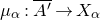 $\mu_{\alpha}: \overline{A'} \rightarrow X_\alpha$
on
$\mu_{\alpha}: \overline{A'} \rightarrow X_\alpha$
on $X_{\alpha}$
by
$X_{\alpha}$
by $\mu_{\alpha}(s) = F_{\alpha}^{-1} \circ \mu(s)$
.
$\mu_{\alpha}(s) = F_{\alpha}^{-1} \circ \mu(s)$
.
By the triangle inequality and the diameter estimate $\text{diam}_{\alpha} (F_{\alpha}^{-1}(\overline{G_i})) \lt \epsilon$
, we have that
$\text{diam}_{\alpha} (F_{\alpha}^{-1}(\overline{G_i})) \lt \epsilon$
, we have that
 \begin{align} d_{\alpha}(p,q) &\leq d(p,\mu_{\alpha}(a_1))+\sum\limits_{i=1}^{\ell} d_{\alpha}(\mu_{\alpha}(a_i),\mu_{\alpha}(b_i)) + \sum\limits_{i=2}^{\ell} d_{\alpha}(\mu_{\alpha}(b_{i-1}),\mu_{\alpha}(a_i)) + d_{\alpha}(\mu_{\alpha}(b_{\ell},q)\nonumber\\ &\leq L_{\alpha}({\mu}_{\alpha}|_{[0,a_1]}) + \sum\limits_{i=2}^{\ell} L_{\alpha}(\mu_{\alpha} \mid_{[b_{i-1},a_i]}) + L_{\alpha}(\mu_{\alpha} \mid_{[b_{\ell},1]})+k\epsilon \nonumber\\ &\leq \int_{A'} |\dot{\mu}_{\alpha}(s)|_{g_{\alpha}}\, ds + k \epsilon = \int_{A'} |(F_{\alpha}^{-1})_* \dot{\mu}(s) |_{g_{\alpha}}\, ds + k \epsilon. \end{align}
The set A’ is defined such that $\mu|_{A'} \in X_0 \setminus \bigcup_i G_i$
. The uniform convergence of the metrics
$\mu|_{A'} \in X_0 \setminus \bigcup_i G_i$
. The uniform convergence of the metrics $(F_{\alpha}^{-1})^*g_{\alpha}$
to
$(F_{\alpha}^{-1})^*g_{\alpha}$
to $g_0$
on this region gives that
$g_0$
on this region gives that
 \begin{equation*} \int_{A'} |(F_{\alpha}^{-1})_* \dot{\mu}(s) |_{g_{\alpha}}\, ds \leq (1+ \delta) \int_{A'} |\dot{\mu}(s) |_{g_0}\, ds \leq (1+\delta) L_0(\mu), \end{equation*}
and $\delta$
can be made arbitrarily small for sufficiently small
$\delta$
can be made arbitrarily small for sufficiently small $\alpha$
. We can next apply (28) and (29) to obtain
$\alpha$
. We can next apply (28) and (29) to obtain
 \begin{equation} \int_{A'} |(F_{\alpha}^{-1})_* \dot{\mu}(s) |_{g_{\alpha}}\, ds \leq L_0(\mu) + \delta \, (\text{diam}_{0}(X_0)+k \epsilon). \end{equation}
Note that $\text{diam}_{0}(X_0)< \infty$
, since it is a union of a smooth geometry on a compact manifold
$\text{diam}_{0}(X_0)< \infty$
, since it is a union of a smooth geometry on a compact manifold $X_0 \setminus \bigcup_i G_i$
with sets
$X_0 \setminus \bigcup_i G_i$
with sets $\overline{G_i}$
of bounded diameter that have non-trivial intersection with
$\overline{G_i}$
of bounded diameter that have non-trivial intersection with $X_0 \setminus \bigcup_i G_i$
. Combining (30) and (31) and choosing
$X_0 \setminus \bigcup_i G_i$
. Combining (30) and (31) and choosing $\delta$
small enough gives
$\delta$
small enough gives
 \begin{equation*} d_\alpha(p,q) \leq L_0(\mu) + (k+1) \epsilon. \end{equation*}
Applying (28) and (29), we then have
 \begin{equation} d_{\alpha}(p,q) \leq d_0(F(p),F(q)) + (2k+1) \epsilon. \end{equation}
We now need to obtain the other side of the desired inequality (27), and the argument is similar. Let $\eta_{\alpha} \colon [0,1] \rightarrow X_{\alpha}$
be a curve such that
$\eta_{\alpha} \colon [0,1] \rightarrow X_{\alpha}$
be a curve such that $\eta_{\alpha}(0) = p$
and
$\eta_{\alpha}(0) = p$
and $\eta_{\alpha}(1) = q$
, and
$\eta_{\alpha}(1) = q$
, and
 \begin{equation*} L_{\alpha}(\eta_{\alpha}) = d_{\alpha}(p,q). \end{equation*}
As before, we use Lemma 4 to replace $\eta_\alpha$
with a curve
$\eta_\alpha$
with a curve $\nu_\alpha$
passing through the bad sets
$\nu_\alpha$
passing through the bad sets $F_\alpha^{-1}(\overline{G_i})$
at most k times. The replacement curve
$F_\alpha^{-1}(\overline{G_i})$
at most k times. The replacement curve $\eta_\alpha:[0,1] \rightarrow X_\alpha$
has the same endpoints
$\eta_\alpha:[0,1] \rightarrow X_\alpha$
has the same endpoints $\nu_{\alpha}$
with
$\nu_{\alpha}$
with $\nu_{\alpha}(0) = p$
,
$\nu_{\alpha}(0) = p$
, $\nu_{\alpha}(1) = q$
and satisfies the length estimate
$\nu_{\alpha}(1) = q$
and satisfies the length estimate
 \begin{equation} L_{\alpha}(\nu_{\alpha}) \leq L_{\alpha}(\eta_{\alpha}) + \sum_{i=1}^k \text{diam}_{\alpha}(F_{\alpha}^{-1}(\overline{G_i})) \leq L_{\alpha}(\eta_{\alpha}) + k \epsilon. \end{equation}
The time interval can be broken into $[0,1] = A_{\alpha} \cup A'_{\alpha}$
as before, where
$[0,1] = A_{\alpha} \cup A'_{\alpha}$
as before, where $\nu_\alpha|_{A'_\alpha} \in X_\alpha \setminus \bigcup F_\alpha^{-1}(G_i)$
.
$\nu_\alpha|_{A'_\alpha} \in X_\alpha \setminus \bigcup F_\alpha^{-1}(G_i)$
.
We now move onto the space $(X_0,d_0)$
. Define a curve
$(X_0,d_0)$
. Define a curve $\nu: \overline{A'_\alpha} \rightarrow X_0$
by
$\nu: \overline{A'_\alpha} \rightarrow X_0$
by $\nu(s) = F_{\alpha} \circ \nu_{\alpha}(s)$
, and apply the triangle inequality as in (30) to obtain
$\nu(s) = F_{\alpha} \circ \nu_{\alpha}(s)$
, and apply the triangle inequality as in (30) to obtain
 \begin{equation} d_0(F(p),F(q)) \leq \int_{A'_\alpha} |\dot{\nu}|_{g_0} ds + k \epsilon = \int_{A'_\alpha} |\dot{\nu}_\alpha |_{F_\alpha^* g_0} ds + k \epsilon. \end{equation}
The convergence of the metrics $(F_{\alpha}^{-1})^* g_{\alpha}$
to
$(F_{\alpha}^{-1})^* g_{\alpha}$
to $g_0$
on
$g_0$
on $X_0 \setminus \bigcup_i G_i$
, and the fact that
$X_0 \setminus \bigcup_i G_i$
, and the fact that $\nu_\alpha|_{A'_\alpha}$
stays within
$\nu_\alpha|_{A'_\alpha}$
stays within $X_\alpha \setminus \bigcup F_\alpha^{-1}(G_i)$
, implies that
$X_\alpha \setminus \bigcup F_\alpha^{-1}(G_i)$
, implies that
 \begin{equation} \int_{A'_\alpha} | \dot{\nu}_{\alpha}(s) |_{F_\alpha^* g_0}\, ds \leq \int_{A'_\alpha} (1+|F_\alpha^* g_0 - g_\alpha|_{g_\alpha} )|\dot{\nu}_\alpha|_{g_\alpha} ds \leq L_\alpha(\nu_\alpha) + \delta \, (\text{diam}_{\alpha}(X_\alpha)+1), \end{equation}
where $\delta$
is small for sufficiently small
$\delta$
is small for sufficiently small $\alpha$
. We can bound uniformly in
$\alpha$
. We can bound uniformly in $\alpha$
the diameter
$\alpha$
the diameter
 \begin{equation*} \text{diam}_{\alpha}(X_\alpha) \leq C. \end{equation*}
For this, note that $(X_\alpha \setminus \bigcup_i F_\alpha^{-1}(G_i), g_\alpha)$
is isometric to
$(X_\alpha \setminus \bigcup_i F_\alpha^{-1}(G_i), g_\alpha)$
is isometric to $(X_0 \setminus \bigcup_i G_i, (F_\alpha^{-1})^*g_\alpha)$
, which has bounded diameter since
$(X_0 \setminus \bigcup_i G_i, (F_\alpha^{-1})^*g_\alpha)$
, which has bounded diameter since $(F_\alpha^{-1})^* g_\alpha \rightarrow g_0$
smoothly uniformly on this region. The remaining piece of the geometry
$(F_\alpha^{-1})^* g_\alpha \rightarrow g_0$
smoothly uniformly on this region. The remaining piece of the geometry $(X_\alpha,g_\alpha)$
, namely the sets
$(X_\alpha,g_\alpha)$
, namely the sets $\bigcup_i F_\alpha^{-1}(\overline{G_i})$
, also have bounded diameter.
$\bigcup_i F_\alpha^{-1}(\overline{G_i})$
, also have bounded diameter.
From here, we can combine (34), (35) and (33) and choose $\delta$
small enough to establish
$\delta$
small enough to establish
 \begin{equation*} d_0(F(p),F(q)) \leq d_\alpha(p,q) + (2k+1) \epsilon.\end{equation*}
Combining this together with (32), we obtain (27) and the lemma holds for the uniform constant $C = 2k+1$
.
$C = 2k+1$
.
4.3 Estimates on the small resolution
In this subsection, we will show how Lemma 5 gives convergence of the families of metrics on the small resolution. In the small-resolution case, the maps $F_\alpha$
are simply the blowdown map
$F_\alpha$
are simply the blowdown map $F: \widehat{X} \to X_0$
, while the sets
$F: \widehat{X} \to X_0$
, while the sets $C_{i,\alpha} \subset \widehat{X}$
are the
$C_{i,\alpha} \subset \widehat{X}$
are the $(-1,-1)$
-curves
$(-1,-1)$
-curves $E_i \simeq \mathbb{P}^1$
, and the sets
$E_i \simeq \mathbb{P}^1$
, and the sets $K_{i,\alpha} \subset X_0$
are the singletons
$K_{i,\alpha} \subset X_0$
are the singletons $K_{i,\alpha} = \{s_i\}$
containing the conifold singularities. At this point, we must check that the diameter estimates (ii) and (iii) appearing in Lemma 5 apply for the small-resolution metrics. Since these are local estimates around the
$K_{i,\alpha} = \{s_i\}$
containing the conifold singularities. At this point, we must check that the diameter estimates (ii) and (iii) appearing in Lemma 5 apply for the small-resolution metrics. Since these are local estimates around the $(-1,-1)$
-curves and around the singularities, we work on the local model
$(-1,-1)$
-curves and around the singularities, we work on the local model $(\widehat{V},\widehat{g}_{\mathrm{co},a})$
. In order to get a handle on bounds pertaining to the ‘tube’
$(\widehat{V},\widehat{g}_{\mathrm{co},a})$
. In order to get a handle on bounds pertaining to the ‘tube’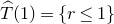 $\widehat{T}(1) = \{ r \leq 1 \}$
, we split it up into a smaller ‘tube’
$\widehat{T}(1) = \{ r \leq 1 \}$
, we split it up into a smaller ‘tube’ $\widehat{T}(aK)$
and an ‘annulus’
$\widehat{T}(aK)$
and an ‘annulus’ $\widehat{T}(1) \backslash \widehat{T}(aK)$
.
$\widehat{T}(1) \backslash \widehat{T}(aK)$
.
4.3.1 Tubular bounds.
Recall the asymptotically conical decay property (CO SR II). We may fix a constant K such that
 \begin{equation*} |(\pi^{-1})^* (\widehat{g}_{\mathrm{co},a}) - g_{\mathrm{co},0}|_{g_{\mathrm{co},0}} \leq \tfrac{1}{2}\end{equation*}
when $r \gt aK$
. We start with uniform bounds on the spaces
$r \gt aK$
. We start with uniform bounds on the spaces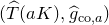 $(\widehat{T}(aK), \widehat{g}_{\mathrm{co},a})$
. These will be obtained using the scaling property (CO SR I) and the compactness of the set
$(\widehat{T}(aK), \widehat{g}_{\mathrm{co},a})$
. These will be obtained using the scaling property (CO SR I) and the compactness of the set $(\widehat{T}(K), \widehat{g}_{\mathrm{co},1})$
.
$(\widehat{T}(K), \widehat{g}_{\mathrm{co},1})$
.
To estimate the diameter, we consider a curve $\gamma \colon [0,1] \rightarrow \widehat{T}(aK)$
. The length of this curve with respect to the metric
$\gamma \colon [0,1] \rightarrow \widehat{T}(aK)$
. The length of this curve with respect to the metric $\widehat{g}_{\mathrm{co},a}$
is given by
$\widehat{g}_{\mathrm{co},a}$
is given by
 \begin{equation*}\begin{aligned} \widehat{L}_{\mathrm{co},a} (\gamma) &= \int_0^1 \sqrt{\widehat{g}_{\mathrm{co},a} ( \dot{\gamma}(s), \dot{\gamma}(s))} \, ds \\ &= \int_0^1 \sqrt{ a^2 \cdot S^*_{a^{-1}} (\widehat{g}_1)( \dot{\gamma}(s), \dot{\gamma}(s) )} \, ds \\ &= a \cdot \int_0^1 \sqrt{ \widehat{g}_{\mathrm{co},1} ( (S_{a^{-1}})_* \dot{\gamma}(s), (S_{a^{-1}})_* \dot{\gamma}(s) )} \, ds \\ &= a \cdot \widehat{L}_{\mathrm{co},1} ( S_{a^{-1}} \circ \gamma ),\end{aligned}\end{equation*}
where we have used (CO SR I). Since there is a one-to-one correspondence between curves in $\widehat{T}(aK)$
and curves in
$\widehat{T}(aK)$
and curves in $\widehat{T}(K)$
given by composition with
$\widehat{T}(K)$
given by composition with $S_{a^{-1}}$
, it follows that
$S_{a^{-1}}$
, it follows that
 \begin{equation} \widehat{\text{diam}}_{\mathrm{co},a} (\widehat{T}(aK)) = a \cdot \widehat{\text{diam}}_{\mathrm{co},1} (\widehat{T}(K)).\end{equation}
To obtain a volume bound, we note that
 \begin{equation*} \widehat{\text{{Vol}}}_{\mathrm{co},a} (\widehat{T}(aK)) = \int_{\widehat{T}(aK)} \widehat{\omega}_{\mathrm{co},a}^3 = \int_{\widehat{T}(aK)} a^6 \cdot S^*_{a^{-1}} (\widehat{\omega}_{\mathrm{co},1}^3).\end{equation*}
Using the change of variables formula, this becomes
 \begin{equation*} \widehat{\text{{Vol}}}_{\mathrm{co},a} (\widehat{T}(aK)) = a^6 \cdot \int_{S_{a^{-1}}(\widehat{T}(aK))} \widehat{\omega}_{\mathrm{co},1}^3 = a^6 \cdot \int_{\widehat{T}(K)} \widehat{\omega}_{\mathrm{co},1}^3 .\end{equation*}
Therefore,
 \begin{equation} \widehat{\text{{Vol}}}_{\mathrm{co},a} (\widehat{T}(aK)) = a^6 \cdot \widehat{\text{{Vol}}}_{\mathrm{co},1} (\widehat{T}(K)).\end{equation}
4.3.2 Annular bounds.
Let $\delta \gt 0$
. We will obtain diameter and volume bounds on the annular region
$\delta \gt 0$
. We will obtain diameter and volume bounds on the annular region $\widehat{T}(\delta) \backslash \widehat{T}(aK)$
for
$\widehat{T}(\delta) \backslash \widehat{T}(aK)$
for $0 \lt a \leq {\delta}/{K}$
. These are derived using the asymptotically conical decay property (CO SR II).
$0 \lt a \leq {\delta}/{K}$
. These are derived using the asymptotically conical decay property (CO SR II).
Fix a point $p = (\lambda, u_0, v_0) \in \widehat{T}(\delta) \backslash \widehat{T}(aK)$
, and denote
$p = (\lambda, u_0, v_0) \in \widehat{T}(\delta) \backslash \widehat{T}(aK)$
, and denote $\rho = r(p)$
. Then
$\rho = r(p)$
. Then $\rho \in (aK,\delta]$
.
$\rho \in (aK,\delta]$
.
Consider the curve $\widehat{\gamma}: [({a}/{\rho})K, 1] \rightarrow \widehat{T}(\delta)$
given by
$\widehat{\gamma}: [({a}/{\rho})K, 1] \rightarrow \widehat{T}(\delta)$
given by
 \begin{equation} \widehat{\gamma}(s) = (\lambda_0, s^{{3}/{2}} u_0, s^{{3}/{2}} v_0).\end{equation}
This path begins in $\widehat{T}(aK)$
and moves along the fiber over
$\widehat{T}(aK)$
and moves along the fiber over $\lambda_0$
to arrive at
$\lambda_0$
to arrive at $p=\widehat{\gamma}(1)$
.
$p=\widehat{\gamma}(1)$
.
Using the blowdown map $\pi: \widehat{V} \rightarrow V_0$
(5), it can be directly checked that this curve is sent to the curve
$\pi: \widehat{V} \rightarrow V_0$
(5), it can be directly checked that this curve is sent to the curve $\gamma = \pi \circ \widehat{\gamma}$
in
$\gamma = \pi \circ \widehat{\gamma}$
in $V_0$
given by
$V_0$
given by
 \begin{equation*} \gamma(s) = s^{{3}/{2}} \cdot \pi(\lambda_0, u_0, v_0).\end{equation*}
It follows that
 \begin{equation*} r (\gamma (s)) = s \cdot \rho.\end{equation*}
Lemma 6. The path $\gamma(s)$
on
$\gamma(s)$
on $V_0$
given above has speed
$V_0$
given above has speed $|\dot{\gamma}|_{g_{\mathrm{co},0}} = \rho$
and length
$|\dot{\gamma}|_{g_{\mathrm{co},0}} = \rho$
and length $L_{\mathrm{co},0}(\gamma)=\rho-aK$
.
$L_{\mathrm{co},0}(\gamma)=\rho-aK$
.
Proof. The cone metric can be written as $g_{\mathrm{co},0} = dr^2 + r^2 \cdot \textrm{pr}_1^* g_L$
, where
$g_{\mathrm{co},0} = dr^2 + r^2 \cdot \textrm{pr}_1^* g_L$
, where $g_L$
is a metric on the link
$g_L$
is a metric on the link $L = \{ r = 1\}$
and
$L = \{ r = 1\}$
and $\textrm{pr}_1: V_0 \rightarrow L$
is the projection to the link
$\textrm{pr}_1: V_0 \rightarrow L$
is the projection to the link $\textrm{pr}_1(z) = {z}/{\| z \|}$
. We can then compute
$\textrm{pr}_1(z) = {z}/{\| z \|}$
. We can then compute
 \begin{equation*}dr (\dot{\gamma}) = \frac{d}{ds} (r \circ \gamma) = \rho\end{equation*}
and
 \begin{equation*} (\textrm{pr}_1)_* \dot{\gamma} = \frac{d}{ds} (\textrm{pr}_1 \circ \gamma) = 0.\end{equation*}
Therefore,
 \begin{equation*} g_{\mathrm{co},0}(\dot{\gamma},\dot{\gamma}) = \rho^2.\end{equation*}
This gives the speed of $\gamma$
, and integration gives the length.
$\gamma$
, and integration gives the length.
We now compare the length of the curve $(\widehat{\gamma}, \widehat{g}_{\mathrm{co},a})$
to the length of the curve
$(\widehat{\gamma}, \widehat{g}_{\mathrm{co},a})$
to the length of the curve $(\gamma, g_{\mathrm{co},0})$
:
$(\gamma, g_{\mathrm{co},0})$
:
 \begin{equation*}\begin{aligned} |\widehat{L}_{\mathrm{co},a}(\widehat{\gamma}) - L_{\mathrm{co},0} (\gamma)| &= \Bigg| \int_{({a}/{\rho})K}^1 |\dot{\widehat{\gamma}}|_{\widehat{g}_{\mathrm{co},a}} - |\dot{\gamma}|_{g_{\mathrm{co},0}} \, ds \Bigg| \\ &\leq \int_{({a}/{\rho)}K}^1 \bigg| |\dot{\widehat{\gamma}}|_{\widehat{g}_{\mathrm{co},a}} - |\dot{\gamma}|_{g_{\mathrm{co},0}} \bigg| \, ds \\ &= \int_{({a}/{\rho})K}^1 \bigg| |\dot{\gamma}|_{(\pi^{-1})* (\widehat{g}_{\mathrm{co},a})} - |\dot{\gamma}|_{g_{\mathrm{co},0}} \bigg| \, ds \\ &= \int_{({a}/{\rho})K}^1 \Bigg| \frac{|\dot{\gamma}|^2_{(\pi^{-1})* (\widehat{g}_{\mathrm{co},a})} - |\dot{\gamma}|^2_{g_{\mathrm{co},0}}}{|\dot{\gamma}|_{(\pi^{-1})* (\widehat{g}_{\mathrm{co},a})} + |\dot{\gamma}|_{g_{\mathrm{co},0}}} \Bigg| \, ds.\end{aligned}\end{equation*}
We then obtain the estimate
 \begin{equation*} \begin{aligned}|\widehat{L}_{\mathrm{co},a}(\widehat{\gamma}) - L_{\mathrm{co},0} (\gamma)| &\leq \int_{({a}/{\rho})K}^1 \frac{| (\pi^{-1})^* \widehat{g}_{\mathrm{co},a} - g_{\mathrm{co},0}|_{g_{\mathrm{co},0}} \, |\dot{\gamma}|_{g_{\mathrm{co},0}}^2}{|\dot{\gamma}|_{(\pi^{-1})* (\widehat{g}_{\mathrm{co},a})} + |\dot{\gamma}|_{g_{\mathrm{co},0}}} \, ds \\&\leq \int_{({a}/{\rho})K}^1 | (\pi^{-1})^* \widehat{g}_{\mathrm{co},a} - g_{\mathrm{co},0}|_{g_{\mathrm{co},0}} \, |\dot{\gamma}|_{g_{\mathrm{co},0}} \, ds. \end{aligned}\end{equation*}
We now use $|\dot{\gamma}|_{g_{\mathrm{co},0}}=\rho$
,
$|\dot{\gamma}|_{g_{\mathrm{co},0}}=\rho$
, $r(\gamma(s)) = s \cdot \rho$
and (CO SR II) to obtain
$r(\gamma(s)) = s \cdot \rho$
and (CO SR II) to obtain
 \begin{equation*}|\widehat{L}_{\mathrm{co},a}(\widehat{\gamma}) - L_{\mathrm{co},0} (\gamma)|\leq \int_{({a}/{\rho})K}^1 \frac{C a^2 \rho}{r^2} \, ds = \frac{Ca^2}{\rho} \cdot \int_{({a}/{\rho})K}^1 \frac{1}{s^2} \, ds = Ca \cdot \Big( \frac{1}{K} - \frac{a}{\rho} \Big).\end{equation*}
Therefore,
 \begin{equation*} \widehat{L}_{\mathrm{co},a}(\widehat{\gamma}) \leq |\widehat{L}_{\mathrm{co},a}(\widehat{\gamma}) - L_{\mathrm{co},0} (\gamma)| + |L_{\mathrm{co},0}(\gamma)| \leq Ca \cdot \Big( \frac{1}{K} - \frac{a}{\rho} \Big) + (\rho - aK).\end{equation*}
For fixed $0 \lt a \leq {\delta}/{K}$
, this is maximized when
$0 \lt a \leq {\delta}/{K}$
, this is maximized when $\rho = \delta$
, giving
$\rho = \delta$
, giving
 \begin{equation*} \widehat{L}_{\mathrm{co},a}(\widehat{\gamma}) \leq C \cdot \Big(\frac{a}{K\delta} + 1\Big) \cdot (\delta - aK) \leq C \cdot (\delta - aK).\end{equation*}
As such, we get
 \begin{equation*} \widehat{d}_{\mathrm{co},a} (p, \widehat{T}(aK)) \leq C \cdot (\delta - aK).\end{equation*}
In tandem with our diameter bound for $\widehat{T}(aK)$
(36), we get
$\widehat{T}(aK)$
(36), we get
 \begin{equation*} \widehat{\text{diam}}_{\mathrm{co},a} (\widehat{T}(\delta)) \leq a \cdot \widehat{\text{diam}}_{\mathrm{co},1} (\widehat{T}(K)) + 2C \cdot (\delta - aK),\end{equation*}
which for fixed $\delta$
and K is uniformly bounded for
$\delta$
and K is uniformly bounded for $0 \lt a \leq {\delta}/{K}$
.
$0 \lt a \leq {\delta}/{K}$
.
In the appendix, we will need a volume estimate on tubes around the exceptional divisor. This volume estimate follows from the diameter estimate and the Bishop–Gromov comparison theorem. Indeed, for $0 \lt a \leq {\delta}/{K}$
, the diameter estimate tells us that
$0 \lt a \leq {\delta}/{K}$
, the diameter estimate tells us that
 \[\widehat{\text{diam}}_{\mathrm{co},a} (\widehat{T}(\delta)) \leq C \delta. \]
Thus, the tube $\widehat{T}(\delta)$
is contained in the ball
$\widehat{T}(\delta)$
is contained in the ball $\widehat{B}(p,C\delta)$
for any point
$\widehat{B}(p,C\delta)$
for any point $p \in \widehat{T}(\delta)$
. Therefore,
$p \in \widehat{T}(\delta)$
. Therefore,
 \begin{align*} \widehat{\text{Vol}}_{\mathrm{co},a}(\widehat{T}(\delta)) &\leq \widehat{\text{Vol}} \, \widehat{B}(p,C\delta) \\ &\leq \text{Vol}_{\mathrm{Euc}} \,B(0,C\delta),\end{align*}
where $\text{Vol}_{\mathrm{Euc}} \, B(0,C\delta)$
denotes the Euclidean volume of the ball of radius
$\text{Vol}_{\mathrm{Euc}} \, B(0,C\delta)$
denotes the Euclidean volume of the ball of radius $C\delta$
in
$C\delta$
in $\mathbb{R}^6$
. This second inequality is by Bishop–Gromov, together with the fact that the metrics
$\mathbb{R}^6$
. This second inequality is by Bishop–Gromov, together with the fact that the metrics $\widehat{g}_{\mathrm{co},a}$
are Ricci-flat. Thus,
$\widehat{g}_{\mathrm{co},a}$
are Ricci-flat. Thus, $ \widehat{\text{Vol}}_{\mathrm{co},a}(\widehat{T}(\delta)) \leq C \delta^6$
. We record these diameter and volume bounds for future reference. The diameter bound is used in the next section, and the volume bound is used in the appendix.
$ \widehat{\text{Vol}}_{\mathrm{co},a}(\widehat{T}(\delta)) \leq C \delta^6$
. We record these diameter and volume bounds for future reference. The diameter bound is used in the next section, and the volume bound is used in the appendix.
Lemma 7. For $\delta \gt 0$
, we have
$\delta \gt 0$
, we have
 \begin{equation} \widehat{\text{diam}}_{\mathrm{co},a} (\widehat{T}(\delta)) \leq C \delta \end{equation}
and
 \begin{equation} \widehat{\textrm {Vol}}_{\mathrm{co},a}(\hat{T}(\delta)) \leq C \delta^6 \end{equation}
for any $0 \lt a \leq {\delta}/{K}$
.
$0 \lt a \leq {\delta}/{K}$
.
4.3.3 Applying the main lemma.
Our diameter estimates will enable us to prove the following useful lemma akin to that of Song and Weinkove [Reference Song and WeinkoveSW13].
Lemma 8. For $0< \epsilon \lt 1$
, there exist
$0< \epsilon \lt 1$
, there exist $\delta \gt 0$
and
$\delta \gt 0$
and $0 \lt a_0$
such that, for
$0 \lt a_0$
such that, for $0 \lt a \lt a_0$
,
$0 \lt a \lt a_0$
,
-
(i)
$\text{diam}_{\mathrm{co},0} (D_0(\delta)) \lt \epsilon$
; and -
(ii)
$\widehat{\text{diam}}_{\mathrm{co},a} (\pi^{-1} (D_0(\delta))) \lt \epsilon$
.


Proof. We have that $D_0(\delta)$
is a closed disc of radius
$D_0(\delta)$
is a closed disc of radius $\delta$
with respect to a cone metric
$\delta$
with respect to a cone metric $g_{\mathrm{co},0} = dr^2 + r^2 \cdot g_L$
. Standard arguments from Riemannian geometry give the diameter of
$g_{\mathrm{co},0} = dr^2 + r^2 \cdot g_L$
. Standard arguments from Riemannian geometry give the diameter of $D_0(\delta)$
to be
$D_0(\delta)$
to be $2 \delta$
. We can then take
$2 \delta$
. We can then take $\delta \lt {\epsilon}/{2}$
to satisfy the first condition.
$\delta \lt {\epsilon}/{2}$
to satisfy the first condition.
Next, we consider the second condition, and note $\pi^{-1}(D_0(\delta)) = \widehat{T}(\delta)$
. Using (39), we see that the result follows once we choose
$\pi^{-1}(D_0(\delta)) = \widehat{T}(\delta)$
. Using (39), we see that the result follows once we choose $\delta$
small enough such that
$\delta$
small enough such that $\delta \lt C^{-1} \epsilon$
,
$\delta \lt C^{-1} \epsilon$
, $\delta \lt {\epsilon}/{2}$
and
$\delta \lt {\epsilon}/{2}$
and $a_0 = {\delta}/{K}$
.
$a_0 = {\delta}/{K}$
.
We can now apply Lemma 5 to prove convergence of the three classes of metrics on the small resolution.
-
– Theorem 2.7. Convergence of the local models
$(\widehat{T}(1),\widehat{d}_{\mathrm{co},a}) \rightarrow (D_0(1), d_{\mathrm{co},0})$
.In this case, we have only one ODP singularity s. By the diameter estimate of
$g_{\mathrm{co},a}$
(Lemma 8), we see that for each
$\epsilon \gt 0$
, we can pick the set
$\overline{G} = D_0(\delta)$
for an appropriately small
$\delta \gt 0$
such that Lemma 5 applies. -
– Theorem 2.8. Convergence of the global balanced metrics
$(\widehat{X}, \widehat{d}_{\mathrm{FLY},a}) \rightarrow (X_0, d_{\mathrm{FLY},0})$
.Here we use the fact that the Fu–Li–Yau metrics are, up to scaling, just the Candelas–de la Ossa metrics in a compact set around the
$(-1,-1)$
-curves
$E_i$
and the ODP singularities
$s_i$
. For
$\epsilon \gt 0$
, we can pick
$\overline{G_i} = D_0(\delta_i)$
for appropriately small
$\delta_i$
around each singular point
$s_i$
. Coupling this with the smooth convergence of the Fu–Li–Yau metrics on compact sets away from the
$(-1,-1)$
-curves, we may apply Lemma 5. -
– Theorem 2.12. Convergence of the global Hermitian Yang–Mills metrics
$(\widehat{X},\widehat{d}_{\widehat{H}_a}) \rightarrow (X_0,d_{H_0})$
.By Proposition 1, we have the estimate
on the local sets
\begin{equation*} C^{-1} \cdot g_{\mathrm{co},a} \leq \widehat{H}_a \leq C \cdot g_{\mathrm{co},a} \end{equation*}
$D_0(\delta_i)$
around each singularity
$s_i$
, where the Fu–Li–Yau metrics are a scaling of the Candelas–de la Ossa metrics. Lemma 8 implies that, for
$\epsilon \gt 0$
, there exist
$\delta_i \gt 0$
and
$a_0 \gt 0$
such that for all
$0 \lt a \lt a_0$
, We may therefore apply Lemma 5.
\begin{equation*} \mathrm{diam}_{H_0}(D_0(\delta_i)) \lt \epsilon, \quad \widehat{\text{diam}}_{\widehat{H}_a}(\pi^{-1} (D_0(\delta_i))) \lt \epsilon. \end{equation*}








4.4 Estimates on the smoothing
We now prove the analogous statements on the smoothings. We will derive diameter bounds on $D_t(\beta_{t,\delta}) \subset V_t$
with respect to
$D_t(\beta_{t,\delta}) \subset V_t$
with respect to $g_{\mathrm{co},t}$
. Volume bounds can also be obtained in a similar way as for the small resolution, and we omit the details as they are not needed in the current work.
$g_{\mathrm{co},t}$
. Volume bounds can also be obtained in a similar way as for the small resolution, and we omit the details as they are not needed in the current work.
We recall that $\beta_{t,\rho}$
is defined by
$\beta_{t,\rho}$
is defined by
 \begin{equation*} \beta_{t,\rho} = \bigg( \rho^3 + \frac{|t|^2}{4 \rho^3} \bigg)^{\!\!{1}/{3}}\end{equation*}
and the role of $\beta_{t,\rho}$
is so that the set
$\beta_{t,\rho}$
is so that the set $\{ r = \beta_{t,\rho} \} \subset V_t$
on the smoothing is identified with the set
$\{ r = \beta_{t,\rho} \} \subset V_t$
on the smoothing is identified with the set $\{ r = \rho \} \subset V_0$
on the cone via the map
$\{ r = \rho \} \subset V_0$
on the cone via the map $\Phi_t$
.
$\Phi_t$
.
The method we will use is analogous to that of the small resolutions. First, we use the asymptotically conical decay property (CO SM II) to set $K \gt 0$
such that
$K \gt 0$
such that
 \begin{equation*} |(\Phi_t)^* (g_{\mathrm{co},t}) - g_{\mathrm{co},0}| \leq \tfrac{1}{2}\end{equation*}
when $r \gt |t|^{{{1}/{3}}}K$
.
$r \gt |t|^{{{1}/{3}}}K$
.
We then split our region of interest $D_t(\beta_{t,\delta})$
into a ‘disc’
$D_t(\beta_{t,\delta})$
into a ‘disc’ $D_t(\beta_{t,|t|^{{{1}/{3}}}K})$
and an ‘annulus’
$D_t(\beta_{t,|t|^{{{1}/{3}}}K})$
and an ‘annulus’ $D_t(\beta_{t,\delta}) \backslash D_t(\beta_{t,|t|^{{{1}/{3}}}K})$
.
$D_t(\beta_{t,\delta}) \backslash D_t(\beta_{t,|t|^{{{1}/{3}}}K})$
.
4.4.1 Bounds on the disc.
We start by estimating the geometry of the disc $D_t(\beta_{t, |t|^{{{1}/{3}}}K})$
. For this, we note that
$D_t(\beta_{t, |t|^{{{1}/{3}}}K})$
. For this, we note that
 \begin{equation*} S_{t^{-{1}/{3}}}: (D_t(\beta_{t,|t|^{{1}/{3}}K}),g_{\mathrm{co},t}) \rightarrow (D_1(\beta_{1,K}), |t|^{{2}/{3}} g_{\mathrm{co},1})\end{equation*}
is an isometry. This is due to the scaling property $g_{\mathrm{co},t} = |t|^{2/3} S^*_{t^{-1/3}}(g_{\mathrm{co},1})$
. It follows that
$g_{\mathrm{co},t} = |t|^{2/3} S^*_{t^{-1/3}}(g_{\mathrm{co},1})$
. It follows that
 \begin{equation} \text{diam}_{\mathrm{co},t} (D_t(\beta_{t,|t|^{{1}/{3}}K})) = |t|^{{1}/{3}} \cdot \text{diam}_{\mathrm{co},1} (D_1(\beta_{1,K})).\end{equation}
4.4.2 Annular bounds.
Let $\delta \gt 0$
. We now compute diameter bounds on the ‘annular’ region
$\delta \gt 0$
. We now compute diameter bounds on the ‘annular’ region $D_t(\beta_{t,\delta}) \backslash D_t(\beta_{t,|t|^{{{1}/{3}}}K})$
when
$D_t(\beta_{t,\delta}) \backslash D_t(\beta_{t,|t|^{{{1}/{3}}}K})$
when $0 \lt |t| \leq ({\delta}/{K})^3$
. As before, this relies on (CO SM II).
$0 \lt |t| \leq ({\delta}/{K})^3$
. As before, this relies on (CO SM II).
Let $q \in D_t(\beta_{t,\delta}) \backslash D_t(\beta_{t, |t|^{{{1}/{3}}}K})$
be an arbitrary point in the annular region. We will construct a curve
$q \in D_t(\beta_{t,\delta}) \backslash D_t(\beta_{t, |t|^{{{1}/{3}}}K})$
be an arbitrary point in the annular region. We will construct a curve $\tilde{\gamma}$
from
$\tilde{\gamma}$
from $D_t(\beta_{t, |t|^{{{1}/{3}}}K})$
to q and estimate its length
$D_t(\beta_{t, |t|^{{{1}/{3}}}K})$
to q and estimate its length $L_{\mathrm{co},t}(\widetilde{\gamma})$
. To do this, we will bring the setup back to the cone
$L_{\mathrm{co},t}(\widetilde{\gamma})$
. To do this, we will bring the setup back to the cone $V_0$
and use a radial ray.
$V_0$
and use a radial ray.
Since $\Phi_t$
is a diffeomorphism on the annular region, we can write
$\Phi_t$
is a diffeomorphism on the annular region, we can write $q = \Phi_t(p)$
for
$q = \Phi_t(p)$
for $p \in V_0$
. We note that
$p \in V_0$
. We note that $\beta$
is defined such that
$\beta$
is defined such that $|t|^{{{1}/{3}}}K \lt r(p) \leq \delta$
and we define
$|t|^{{{1}/{3}}}K \lt r(p) \leq \delta$
and we define $\rho\gt 0$
by
$\rho\gt 0$
by $r(p) = \rho$
. Hence,
$r(p) = \rho$
. Hence,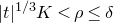 $|t|^{1/3} K \lt \rho \leq \delta$
.
$|t|^{1/3} K \lt \rho \leq \delta$
.
We can define a path $\gamma \colon [|t|^{{{1}/{3}}} {K}/{\rho}, 1] \rightarrow V_0$
by
$\gamma \colon [|t|^{{{1}/{3}}} {K}/{\rho}, 1] \rightarrow V_0$
by
 \begin{equation} \gamma(s) = s^{{3}/{2}} \cdot p.\end{equation}
This path is chosen such that it begins in $D_0(|t|^{{{1}/{3}}}K)$
and moves outward along a ray emanating from 0 to reach
$D_0(|t|^{{{1}/{3}}}K)$
and moves outward along a ray emanating from 0 to reach $\gamma(1) = p$
. It can be checked that
$\gamma(1) = p$
. It can be checked that
 \begin{equation*} \dot{\gamma}(s) = \rho \cdot \frac{\partial }{\partial r} \text{ and } r(\gamma(s)) = \rho \cdot s.\end{equation*}
The corresponding path in $V_t$
is
$V_t$
is $\tilde{\gamma} = \Phi_t \circ \gamma$
, and our goal is to estimate its length. We start with
$\tilde{\gamma} = \Phi_t \circ \gamma$
, and our goal is to estimate its length. We start with
 \begin{equation*}\begin{aligned} |L_{\mathrm{co},t}(\widetilde{\gamma}) - L_{\mathrm{co},0}(\gamma)| &\leq \int_{|t|^{1/3} {K}/{\rho}}^1 \Bigg| |\dot{\gamma}|_{(\Phi_t)^* (g_{\mathrm{co},t})} - |\dot{\gamma}|_{g_{\mathrm{co},0}} \Bigg| \, ds \\ &\leq \int_{|t|^{1/3} {K}/{\rho}}^1 |(\Phi_t)^* g_{\mathrm{co},t} - g_{\mathrm{co},0}|_{g_{\mathrm{co},0}} |\dot{\gamma}|_{g_{\mathrm{co},0}} \, ds.\end{aligned}\end{equation*}
Using $|\dot{\gamma}|_{g_{\mathrm{co},0}} = \rho$
,
$|\dot{\gamma}|_{g_{\mathrm{co},0}} = \rho$
, $r(s) = s \cdot \rho$
and (CO SR II), we get
$r(s) = s \cdot \rho$
and (CO SR II), we get
 \begin{equation*} |L_{\mathrm{co},t}(\widetilde{\gamma}) - L_{\mathrm{co},0}(\gamma)| \leq C \int_{|t|^{1/3} {K}/{\rho}}^1 |t| r^{-3}(s) \rho \, ds \leq C \bigg( \frac{|t|^{1/3}}{K^2} - \frac{|t|}{\rho^2} \bigg).\end{equation*}
We can also check that
 \begin{equation*} L_{\mathrm{co},0} (\gamma) = \int_{|t|^{1/3} {K}/{\rho}}^1 \rho \, ds = \rho - |t|^{1/3} K.\end{equation*}
By the triangle inequality and the above estimates, we conclude
 \begin{equation*} L_{\mathrm{co},t}(\widetilde{\gamma}) \leq C( \rho + |t|^{1/3} K^{-2}).\end{equation*}
Since $|t| \leq \delta^3 K^{-3}$
and
$|t| \leq \delta^3 K^{-3}$
and $\rho \leq \delta$
, we conclude that
$\rho \leq \delta$
, we conclude that
 \begin{equation} d_{\mathrm{co},t}(q, D_t(\beta_{t,|t|^{{1}/{3}}K})) \leq C \delta.\end{equation}
Combining this with our diameter bound (41) for $D_t(\beta_{t,|t|^{{{1}/{3}}}K})$
, we get
$D_t(\beta_{t,|t|^{{{1}/{3}}}K})$
, we get
 \begin{equation} \text{diam}_{\mathrm{co},t} ( D_t(\beta_{t,\delta})) \leq C \delta, \quad 0 \lt |t| \leq \frac{\delta^3}{K^3},\end{equation}
which is the desired diameter bound for the Calabi–Yau metrics on the local model $(V_t,g_{\mathrm{co},t})$
.
$(V_t,g_{\mathrm{co},t})$
.
4.4.3 Bounds for the Fu–Li–Yau metrics.
On the smoothings, the Fu–Li–Yau metrics are only close to scaled Candelas–de la Ossa metrics instead of being exactly equal to them. Owing to this, we require a version of the diameter bound (44) for the Fu–Li–Yau metric. This will follow by virtue of the estimate (13).Consider a curve $\gamma$
on the disc
$\gamma$
on the disc $D_t(\beta_{t,\delta})$
. We compare the length of this path
$D_t(\beta_{t,\delta})$
. We compare the length of this path $\gamma$
with respect to the Fu–Li–Yau metric and to a scaled Candelas–de la Ossa metric:
$\gamma$
with respect to the Fu–Li–Yau metric and to a scaled Candelas–de la Ossa metric:
 \begin{equation*} |L_{\mathrm{FLY},t}(\gamma) - \sqrt{c} \cdot L_{\mathrm{co},t}(\gamma)| \leq \frac{1}{\sqrt{c}} \int_{0}^1 |g_{\mathrm{FLY},t} - c \cdot g_{\mathrm{co},t}|_{g_{\mathrm{co},t}} \cdot |\dot{\gamma}|_{g_{\mathrm{co},t}} \, ds.\end{equation*}
Using (13), and recognizing that the $0<\delta<1$
and
$0<\delta<1$
and $K \gg 1$
appearing here can be chosen such that
$K \gg 1$
appearing here can be chosen such that $\beta_{t,\delta}$
is smaller than the
$\beta_{t,\delta}$
is smaller than the $\delta$
appearing in (13) for all
$\delta$
appearing in (13) for all $0 \lt |t| \leq ({\delta}/{K})^3$
, we have
$0 \lt |t| \leq ({\delta}/{K})^3$
, we have
 \begin{equation*} |L_{\mathrm{FLY},t}(\gamma) - \sqrt{c} \cdot L_{\mathrm{co},t}(\gamma)| \leq C |t|^{{2}/{3}} \, L_{\mathrm{co},t}(\gamma).\end{equation*}
Thus,
 \begin{equation*} L_{\mathrm{FLY},t}(\gamma) \leq C(|t|^{{2}/{3}}+1) \, L_{\mathrm{co},t}(\gamma).\end{equation*}
It then follows that
 \begin{equation*} \text{diam}_{\mathrm{FLY},t} (D_t(\beta_{t,\delta})) \leq C (|t|^{{2}/{3}} +1) \text{diam}_{\mathrm{co},t} ( D_t(\beta_{t,\delta})).\end{equation*}
Combining this with (44), we have the following.
Lemma 9. For $\delta \gt 0$
,
$\delta \gt 0$
,
 \begin{equation} \text{diam}_{\mathrm{FLY},t} (D_t(\beta_{t,\delta})) \leq C \delta (|t|^{{2}/{3}}+1), \end{equation}
for all $0 \lt |t| \leq ({\delta}/{K})^3$
.
$0 \lt |t| \leq ({\delta}/{K})^3$
.
4.4.4 Applying the main lemma.
Using the diameter estimates, we prove an analog of Lemma 8 in the case of the smoothings for the Candelas–de la Ossa and Fu–Li–Yau metrics.
Lemma 10. For $0 \lt \epsilon \lt 1$
, there exists
$0 \lt \epsilon \lt 1$
, there exists $\delta \gt 0$
and
$\delta \gt 0$
and $0 \lt t_0$
such that, for
$0 \lt t_0$
such that, for $0 \lt |t| \lt t_0$
,
$0 \lt |t| \lt t_0$
,
-
(i)
$\text{diam}_{\mathrm{co},0} (D_0(\delta)) < \epsilon$
; and
-
(ii)
$\text{diam}_{\mathrm{co},t} (D_t(\beta_{t,\delta})) \lt \epsilon$
.


The result also holds when taking diameters with respect to the Fu–Li–Yau metrics $g_{\mathrm{FLY},0}$
and
$g_{\mathrm{FLY},0}$
and $g_{\mathrm{FLY},t}$
instead of the Candelas–de la Ossa metrics
$g_{\mathrm{FLY},t}$
instead of the Candelas–de la Ossa metrics $g_{\mathrm{co},0}$
and
$g_{\mathrm{co},0}$
and $g_{\mathrm{co},t}$
.
$g_{\mathrm{co},t}$
.
Proof. As was the case in Lemma 8, the first condition holds as long as $\delta \lt {\epsilon}/{2}$
. Using (44) or (45), we see that for all
$\delta \lt {\epsilon}/{2}$
. Using (44) or (45), we see that for all $0 \lt |t| \leq ({\delta}/{K})^3$
, we have the estimate
$0 \lt |t| \leq ({\delta}/{K})^3$
, we have the estimate
 \begin{equation} \text{diam}_{\mathrm{co},t} ( D_t(\beta_{t,\delta})) \leq C \delta \end{equation}
for some uniform constant $C \gt 0$
. The result follows.
$C \gt 0$
. The result follows.
Applying our lemma then gives convergence of our metrics on the smoothings.
-
– Convergence of the local models
$(D_t(\beta_{t,1}), d_{\mathrm{co},t}) \rightarrow (D_0(1), d_{\mathrm{co},0})$
.We have only one ODP singularity s for this case. Using our diameter estimate (44), we have that for
$\epsilon \gt 0$
, we can pick
$\overline{G} = D_0(\delta)$
,
$K_t = D_0(({|t|}/{2})^{{{1}/{3}}})$
and
$C_t = D_t(|t|^{{{1}/{3}}})$
for sufficiently small
$\delta \gt 0$
and t such that Lemma 5 applies with the maps
$\Phi_t$
. -
– Convergence of the global balanced metrics
$(X_t,d_{\mathrm{FLY},t}) \rightarrow (X_0, d_{\mathrm{FLY},0})$
.Here, we use the diameter estimate (45) instead. For
$\epsilon \gt 0$
, we can again pick
$\overline{G_i} = D_0(\delta_i)$
,
$K_{i,t} = D_0(({|t|}/{2})^{{{1}/{3}}})$
and
$C_{i,t} = D_t(|t|^{{{1}/{3}}})$
for sufficiently small
$\delta_i \gt 0$
and t around each singularity
$s_i$
. As such, we can apply the lemma with the maps
$\Phi_t$
. -
– Convergence of the global Hermitian Yang–Mills metrics
$(X_t,d_{H_t}) \rightarrow (X_0,d_{H_0})$
.Similar to the case of the small resolutions, we use estimate (14), which is
on the local sets
\begin{equation} C^{-1} \cdot g_{\mathrm{FLY},t} \leq H_t \leq C \cdot g_{\textrm{FLY,t}} \end{equation}
$D_0(\delta_i)$
around the singularities
$s_i$
. Set
$K_{i,t} = D_0(({|t|}/{2})^{{{1}/{3}}})$
and
$C_{i,t} = D_t(|t|^{{{1}/{3}}})$
. Lemma 10 then gives that, for
$\epsilon \gt 0$
, there exists
$\delta_i \gt 0$
and
$t_0 \gt 0$
such that for all
$0 \lt |t| \lt t_0$
, Applying Lemma 5 using the maps
\begin{equation} \text{diam}_{H_0} (D_0(\delta_i)) \lt \epsilon, \quad \text{diam}_{H_t} (D_t(\beta_{t,\delta_i})) \lt \epsilon. \end{equation}
$\Phi_t$
proves the result.



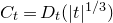








Combining these results with the analogous results for the small resolution found at the end of §4.3.2, we obtain Theorem 4.1.
Appendix A. Hermitian–Yang–Mills metrics on the resolution
The presentation in [Reference Collins, Picard and YauCPY24] only uses convergence of Hermitian Yang–Mills metrics along a subsequence of the Fu–Li–Yau metrics $\widehat{\omega}_{\mathrm{FLY},a_k}$
as
$\widehat{\omega}_{\mathrm{FLY},a_k}$
as $a_k \rightarrow 0$
. Convergence along the full sequence
$a_k \rightarrow 0$
. Convergence along the full sequence $a \rightarrow 0$
also follows from the estimates in [Reference Collins, Picard and YauCPY24], and in this appendix we provide the full details.
$a \rightarrow 0$
also follows from the estimates in [Reference Collins, Picard and YauCPY24], and in this appendix we provide the full details.
We start by establishing notation. We denote the components of a Hermitian metric H on $T^{1,0}X$
by
$T^{1,0}X$
by $H_{\alpha \bar{\beta}}$
, and this convention is such that the associated inner product on
$H_{\alpha \bar{\beta}}$
, and this convention is such that the associated inner product on $T^{1,0}X$
is given by
$T^{1,0}X$
is given by
 \begin{equation*}\langle u, v \rangle = u^\alpha H_{\alpha \bar{\beta}} \overline{v^\beta}, \quad u, v \in \Gamma(T^{1,0}X).\end{equation*}
The components of the inverse of H are denoted $H^{\bar{\mu} \nu}$
, so that
$H^{\bar{\mu} \nu}$
, so that $H_{\mu \bar{\nu}} H^{\bar{\nu} \kappa} = \delta_\mu{}^\kappa$
. The Chern connection associated to H will be denoted
$H_{\mu \bar{\nu}} H^{\bar{\nu} \kappa} = \delta_\mu{}^\kappa$
. The Chern connection associated to H will be denoted $\nabla$
, so that
$\nabla$
, so that
 \begin{equation*}\nabla_k u^\alpha = \partial_k u^\alpha + u^\beta (\partial_k H_{\beta \bar{\gamma}} H^{\bar{\gamma} \alpha}), \quad \nabla_{\bar{k}} u^\alpha = \partial_{\bar{k}} u^\alpha.\end{equation*}
The Chern curvature of H will be denoted by $F \in \Lambda^{1,1}(\textrm{End} \, T^{1,0}X)$
with conventions
$F \in \Lambda^{1,1}(\textrm{End} \, T^{1,0}X)$
with conventions
 \begin{equation*} F_\beta{}^\alpha{}_{j \bar{k}} = -\partial_{\bar{k}} (\partial_j H_{\beta \bar{\gamma}} H^{\bar{\gamma} \alpha}).\end{equation*}
We often omit the endomorphism indices and write $F_{j \bar{k}} = - \partial_{\bar{k}}(\partial_j H H^{-1})$
. Given two metrics H and
$F_{j \bar{k}} = - \partial_{\bar{k}}(\partial_j H H^{-1})$
. Given two metrics H and $\hat{H}$
, the difference in curvature tensors is
$\hat{H}$
, the difference in curvature tensors is
 \begin{equation} (F_H)_{j \bar{k}} - (F_{\hat{H}})_{j \bar{k}} = - \partial_{\bar{k}} (\hat{\nabla}_j h h^{-1}), \quad h = H \hat{H}^{-1},\end{equation}
where $\hat{\nabla} h = \partial h + [h,\partial \hat{H} \hat{H}^{-1}]$
is the induced connection on
$\hat{\nabla} h = \partial h + [h,\partial \hat{H} \hat{H}^{-1}]$
is the induced connection on $\textrm{End} \, T^{1,0}X$
.
$\textrm{End} \, T^{1,0}X$
.
Let $\omega_a = i (g_a)_{j \bar{k}} dz^j \wedge d \bar{z}^k$
be the sequence of Fu–Li–Yau balanced metrics on the resolution
$\omega_a = i (g_a)_{j \bar{k}} dz^j \wedge d \bar{z}^k$
be the sequence of Fu–Li–Yau balanced metrics on the resolution $\hat{X}$
. To ease notation, in this section we write
$\hat{X}$
. To ease notation, in this section we write $\omega_a$
instead of
$\omega_a$
instead of $\widehat{\omega}_{\mathrm{FLY},a}$
. We will use the notation
$\widehat{\omega}_{\mathrm{FLY},a}$
. We will use the notation
 \begin{equation*} \sqrt{-1} \Lambda_\omega F = g^{j \bar{k}} F_{j \bar{k}}.\end{equation*}
From [Reference Collins, Picard and YauCPY24], there is a sequence $H_a$
of Hermitian Yang–Mills metrics on
$H_a$
of Hermitian Yang–Mills metrics on $T^{1,0}X$
solving
$T^{1,0}X$
solving
 \begin{equation*} \sqrt{-1} \Lambda_{\omega_a} F_{H_a} = 0,\end{equation*}
along with estimates
 \begin{equation} C^{-1} g_a \leq H_a \leq C g_a, \quad r |\nabla H_a|_{g_a} \leq C,\end{equation}
where the constants are uniform in a. Furthermore, for each $K \subseteq \hat{X} \setminus E$
there are estimates
$K \subseteq \hat{X} \setminus E$
there are estimates
 \begin{equation*} \sup_K |\nabla^j H_a|_{g_a} \leq C(K,j).\end{equation*}
We first normalize the sequence $\{ H_a \}$
. We define
$\{ H_a \}$
. We define
 \begin{equation*} f_a := \log \frac{\det H_a}{\det g_a},\end{equation*}
and after replacing $H_a$
with
$H_a$
with $e^{-c_a} H_a$
, we can fix the normalization
$e^{-c_a} H_a$
, we can fix the normalization
 \begin{equation} \int_{\hat{X}} f_a \, d \textrm {vol}_{g_a} = 0.\end{equation}
Since $C^{-1} g_a \leq H_a \leq C g_a$
, the constants
$C^{-1} g_a \leq H_a \leq C g_a$
, the constants $e^{-c_a}$
are uniformly bounded, and so the normalized sequence
$e^{-c_a}$
are uniformly bounded, and so the normalized sequence $\{ H_a \}$
still satisfies the estimates (A.2). By the Arzelà–Ascoli theorem, for each
$\{ H_a \}$
still satisfies the estimates (A.2). By the Arzelà–Ascoli theorem, for each $K \subset \hat{X} \setminus E$
there is a subsequence
$K \subset \hat{X} \setminus E$
there is a subsequence $H_{b_i} \rightarrow H_0$
converging uniformly. Taking an exhaustion of compact sets and identifying
$H_{b_i} \rightarrow H_0$
converging uniformly. Taking an exhaustion of compact sets and identifying $\hat{X} \setminus E$
with
$\hat{X} \setminus E$
with $(X_0)_\textrm{reg}$
, we obtain a subsequence
$(X_0)_\textrm{reg}$
, we obtain a subsequence $H_{b_i} \rightarrow H_0$
which converges pointwise on
$H_{b_i} \rightarrow H_0$
which converges pointwise on $(X_0)_\textrm{reg}$
and uniformly on compact subsets.
$(X_0)_\textrm{reg}$
and uniformly on compact subsets.
The goal of this appendix is to upgrade the subsequential convergence to convergence of the full sequence $\{ H_a \}$
uniformly on compact subsets of
$\{ H_a \}$
uniformly on compact subsets of $(X_0)_\textrm{reg}$
.
$(X_0)_\textrm{reg}$
.
Lemma 11. For any compact sets $K \subseteq \widehat{X} \setminus E$
, we have convergence
$K \subseteq \widehat{X} \setminus E$
, we have convergence
 \[H_a \rightarrow H_0 \]
in the $C^\ell(K)$
norm for any integer
$C^\ell(K)$
norm for any integer $\ell$
.
$\ell$
.
We proceed by contradiction. Suppose not, so that there exists an $\epsilon\gt 0$
, a compact subset
$\epsilon\gt 0$
, a compact subset $K_0 \subseteq (X_0)_\textrm{reg}$
, and a subsequence
$K_0 \subseteq (X_0)_\textrm{reg}$
, and a subsequence $a_i \rightarrow 0$
with
$a_i \rightarrow 0$
with
 \begin{equation} \sup_{K_0} |H_{a_i} - H_0|_{g_0} \geq \epsilon\end{equation}
for all $a_i$
. We can apply the estimates (A.2) and the Arzelà–Ascoli theorem to the
$a_i$
. We can apply the estimates (A.2) and the Arzelà–Ascoli theorem to the $\{H_{a_i} \}$
to extract a further subsequence
$\{H_{a_i} \}$
to extract a further subsequence $\{ H_{a_{i_k}} \}$
converging uniformly to a limit
$\{ H_{a_{i_k}} \}$
converging uniformly to a limit $\tilde{H}_0$
on compact subsets of
$\tilde{H}_0$
on compact subsets of $(X_0)_\textrm{reg}$
.
$(X_0)_\textrm{reg}$
.
We now have two limiting metrics $H_0$
and
$H_0$
and $\tilde{H}_0$
. Our goal will be to show that
$\tilde{H}_0$
. Our goal will be to show that $H_0=\tilde{H}_0$
. Taking the limit of (A.4) along the subsequence
$H_0=\tilde{H}_0$
. Taking the limit of (A.4) along the subsequence $a_{i_k}$
gives
$a_{i_k}$
gives
 \begin{equation*} \sup_{K_0} |\tilde{H}_0 - H_0|_{g_0} \geq \epsilon,\end{equation*}
which is the desired contradiction.
The main step in showing $H_0 = \tilde{H}_0$
is the following.
$H_0 = \tilde{H}_0$
is the following.
Lemma 12. Equip $(X_0)_\textrm{reg}$
with the Fu–Li–Yau metric
$(X_0)_\textrm{reg}$
with the Fu–Li–Yau metric $g_0$
. Let
$g_0$
. Let $H_0$
and
$H_0$
and $\tilde{H}_0$
be two metrics on the holomorphic tangent bundle of
$\tilde{H}_0$
be two metrics on the holomorphic tangent bundle of $(X_0)_\textrm{ reg}$
, each satisfying
$(X_0)_\textrm{ reg}$
, each satisfying
 \begin{equation} \omega_0^2 \wedge F_{H} = 0, \quad C^{-1} \cdot g_0 \leq H \leq C \cdot g_0, \quad r |\nabla H|_{g_0} \leq C.\end{equation}
Then $H_0 = \lambda \tilde{H}_0$
for a constant
$H_0 = \lambda \tilde{H}_0$
for a constant $\lambda \in \mathbb{C}$
.
$\lambda \in \mathbb{C}$
.
We will prove Lemma 12 below, but let us assume it for now and complete the argument. Combining Lemma 12 with the normalization condition (A.6) proved below, we obtain the uniqueness $H_0 = \tilde{H}_0$
. This completes the proof of Lemma 11.
$H_0 = \tilde{H}_0$
. This completes the proof of Lemma 11.
The normalization (A.3) along the sequence leads to the following normalization for the limit.
Lemma 13. Set $e^u = \tilde{H}_0 H_0^{-1}$
. Then
$e^u = \tilde{H}_0 H_0^{-1}$
. Then
 \begin{equation} \int_{(X_0)_\textrm{reg}} (\mathrm{Tr} \, u) \, d \textrm {vol}_{g_0} = 0.\end{equation}
Proof. We have two subsequences $\{ b_i \}$
and
$\{ b_i \}$
and $\{ a_i \}$
such that
$\{ a_i \}$
such that $f_{b_i} \rightarrow f_0$
and
$f_{b_i} \rightarrow f_0$
and $f_{a_i} \rightarrow \tilde{f}_0$
pointwise on
$f_{a_i} \rightarrow \tilde{f}_0$
pointwise on $\hat{X} \setminus E$
and uniformly on compact sets. Taking the logarithm of
$\hat{X} \setminus E$
and uniformly on compact sets. Taking the logarithm of
 \begin{equation*} \frac{\det \tilde{H}_0}{\det g_0} = (\det e^u) \frac{\det H_0}{\det g_0},\end{equation*}
we have $\tilde{f}_0 = \mathrm{Tr} \, u + f_0$
. Thus, if we can show that
$\tilde{f}_0 = \mathrm{Tr} \, u + f_0$
. Thus, if we can show that
 \begin{equation*} \int_{(X_0)_\textrm{reg}} f_0 \, d \textrm {vol}_{g_0} = 0, \quad \int_{(X_0)_\textrm{reg}} \tilde{f}_0 \, d \textrm {vol}_{g_0} = 0,\end{equation*}
we will have established (A.6). The calculation of both these integrals is the same, so we only calculate for the sequence $\{ b_i \}$
. We split the integral as
$\{ b_i \}$
. We split the integral as
 \begin{equation*} \int_{(X_0)_\textrm{reg}} f_0 \, d \textrm {vol}_{g_0} = \int_{\{r \lt \delta \}} f_0 \, d \textrm {vol}_{g_0}+ \int_{ \{ r \geq \delta \}} f_0 \, d \textrm {vol}_{g_0}.\end{equation*}
The first integral can be estimated by using $|f_0| \leq C$
(A.5), so that
$|f_0| \leq C$
(A.5), so that
 \begin{align*} \bigg| \int_{\{r \lt \delta \}} f_0 \, d \textrm {vol}_{g_0} \bigg| &\leq C \int_{\{r \lt \delta \}} d \textrm {vol}_{g_0} \leq C \delta^6.\end{align*}
The second integral can be estimated by passing the limit under the integral over compact sets and using $\int_X f_i \, d \textrm {vol}_{g_i} = 0$
:
$\int_X f_i \, d \textrm {vol}_{g_i} = 0$
:
 \begin{align*} \bigg| \int_{\{r \geq \delta \}} f_0 \, d \textrm {vol}_{g_0} \bigg| &= \lim_{b_i \rightarrow 0} \bigg| \int_{\{r \geq \delta \}} f_{b_i} d \textrm{ vol}_{g_{b_i}} \bigg|\nonumber\\ &= \lim_{b_i \rightarrow 0}\bigg| \int_{\{r \lt \delta \}} f_{b_i} d \textrm {vol}_{g_{b_i}} \bigg| \nonumber\\ &\leq C \limsup_{b_i \rightarrow 0} \textrm {Vol}_{\mathrm{co},b_i} (\hat{T}(\delta)).\end{align*}
Here we used $C^{-1} g_b \leq H_b \leq C g_b$
implies
$C^{-1} g_b \leq H_b \leq C g_b$
implies $|f_b|\leq C$
. We use the volume estimate (40) to conclude
$|f_b|\leq C$
. We use the volume estimate (40) to conclude
 \begin{equation*} \limsup_{b_i \rightarrow 0} \textrm {Vol}_{\mathrm{co},b_i} (\hat{T}(\delta)) \leq C \delta^6.\end{equation*}
We can now send $\delta \rightarrow 0$
to complete the proof of the lemma.
$\delta \rightarrow 0$
to complete the proof of the lemma.
All that remains now is to prove Lemma 12. We need to show that $h = \tilde{H}_0 H_0^{-1}$
is a multiple of the identity endomorphism. Taking the trace of (A.1) and using the Hermitian Yang–Mills equation gives the following equation for h:
$h = \tilde{H}_0 H_0^{-1}$
is a multiple of the identity endomorphism. Taking the trace of (A.1) and using the Hermitian Yang–Mills equation gives the following equation for h:
 \begin{equation} (g_0)^{j \bar{k}} \partial_{\bar{k}} ((\nabla^{H_0})_j h h^{-1}) = 0.\end{equation}
The following key identity was observed by Uhlenbeck and Yau [Reference Uhlenbeck and YauUY86]. We will use a version from Jacob and Walpuski [Reference Jacob and WalpuskiJW18] and give the proof for completeness.
Lemma 14. Let $H= e^u \hat{H}$
be a pair of Hermitian metrics on a holomorphic bundle
$H= e^u \hat{H}$
be a pair of Hermitian metrics on a holomorphic bundle $E \rightarrow X$
over a Hermitian manifold (X,g). Write
$E \rightarrow X$
over a Hermitian manifold (X,g). Write $h = e^u$
. Then we have the identity
$h = e^u$
. Then we have the identity
 \begin{equation} \Delta_g |u|^2_{\hat{H}} = 2 \langle g^{\bar{k} j} \partial_{\bar{k}} (\hat{\nabla}_j h h^{-1}), u \rangle_{\hat{H}} + 2 g^{\bar{k} j} \langle \hat{\nabla}_j h h^{-1}, \hat{\nabla}_k u \rangle_{\hat{H}}. \end{equation}
If we assume $|u|_{\hat{H}} \leq R$
, then there exists a constant
$|u|_{\hat{H}} \leq R$
, then there exists a constant $C(R)\gt 0$
such that the following estimate holds:
$C(R)\gt 0$
such that the following estimate holds:
 \begin{equation} \Delta_g |u|^2_{\hat{H}} \geq 2 \langle g^{j \bar{k}} \partial_{\bar{k}} (\hat{\nabla}_j h h^{-1}), u \rangle_{\hat{H}} + \frac{1}{C} |\hat{\nabla} u|^2_{\hat{H}}. \end{equation}
Proof. We start by recalling the definition of u. Let $\{ e_a \}$
be a local smooth frame for
$\{ e_a \}$
be a local smooth frame for $T^{1,0}X$
such that
$T^{1,0}X$
such that
 \begin{equation*}\hat{H} = \sum_{a=1}^3 e^a \otimes \overline{e^a}, \quad h = \sum_{a=1}^3 \lambda_a \, e_a \otimes e^a.\end{equation*}
Then u is defined by
 \begin{equation*} u = \sum_{a=1}^3 (\log \lambda_a) \, e_a \otimes e^a.\end{equation*}
In this frame, the adjoint $\dagger$
with respect to
$\dagger$
with respect to $\hat{H}$
is just the conjugate-transpose of the components, and so
$\hat{H}$
is just the conjugate-transpose of the components, and so $h^\dagger = h$
and
$h^\dagger = h$
and $u^\dagger =u$
.
$u^\dagger =u$
.
The connection coefficients are $\hat{\nabla}_i e_a = A_{i a}{}^b e_b$
and metric compatibility implies
$\hat{\nabla}_i e_a = A_{i a}{}^b e_b$
and metric compatibility implies $A_{i a}{}^b = -\overline{A_{\bar{i} b}{}^a}$
. We can then compute
$A_{i a}{}^b = -\overline{A_{\bar{i} b}{}^a}$
. We can then compute
 \begin{equation*}(\hat{\nabla}_i u)_a{}^b = \frac{\partial_i \lambda_a}{\lambda_a} \delta_a{}^b + (\log \lambda_a - \log \lambda_b) A_{ia}{}^b\end{equation*}
and
 \begin{equation*}(\hat{\nabla}_i h h^{-1})_a{}^b = \frac{\partial_i \lambda_a}{\lambda_a} \delta_a{}^b + \lambda_b^{-1}(\lambda_a-\lambda_b) A_{ia}{}^b.\end{equation*}
The inner product on endomorphisms is $\langle u,v \rangle_{\hat{H}} = \mathrm{Tr} \, u v^\dagger_{\hat{H}}$
, and to ease notation we drop the subscript
$\langle u,v \rangle_{\hat{H}} = \mathrm{Tr} \, u v^\dagger_{\hat{H}}$
, and to ease notation we drop the subscript $\hat{H}$
. We have
$\hat{H}$
. We have
 \begin{equation*} \partial_i |u|^2 = \langle \hat{\nabla}_i u,u \rangle + \langle u, \hat{\nabla}_{\bar{i}} u \rangle = 2 \langle \hat{\nabla}_i u, u \rangle,\end{equation*}
since $u^\dagger = u$
and
$u^\dagger = u$
and $(\nabla_{\bar{i}} u)^\dagger = \hat{\nabla}_i u$
. Furthermore, we notice that the expressions above imply
$(\nabla_{\bar{i}} u)^\dagger = \hat{\nabla}_i u$
. Furthermore, we notice that the expressions above imply
 \begin{equation*} \langle \hat{\nabla}_i u, u \rangle = \langle \hat{\nabla}_i h h^{-1}, u \rangle,\end{equation*}
since the inner product only picks up the diagonal part. Therefore,
 \begin{equation*}\begin{aligned}g^{\bar{k} j} \partial_{\bar{k}} \partial_j |u|^2 &= 2 g^{\bar{k} j} \partial_{\bar{k}} \langle \hat{\nabla}_j h h^{-1}, u \rangle \nonumber\\&= 2 \langle g^{\bar{k} j} \partial_{\bar{k}} (\hat{\nabla}_j h h^{-1}), u \rangle + 2 g^{\bar{k} j} \langle \hat{\nabla}_j h h^{-1}, \hat{\nabla}_k u \rangle.\end{aligned}\end{equation*}
This proves identity (A.8). For the estimate, it remains to show
 \begin{equation} g^{\bar{k} j} \langle \hat{\nabla}_j h h^{-1}, \hat{\nabla}_k u \rangle \geq \tfrac{1}{C} g^{\bar{k} j} \langle \hat{\nabla}_j u, \hat{\nabla}_k u \rangle.\end{equation}
We compute
 \begin{equation*} \langle \hat{\nabla}_j h h^{-1}, \hat{\nabla}_k u \rangle = (\hat{\nabla}_j h h^{-1})_a{}^b (\hat{\nabla}_{\bar{k}} u)_b{}^a,\end{equation*}
which gives
 \begin{equation*} \langle \hat{\nabla}_j h h^{-1}, \hat{\nabla}_k u \rangle = \sum_{a,b} \partial_j \log \lambda_a \partial_{\bar{k}} \log \lambda_a + \log \frac{\lambda_a}{\lambda_b} \lambda_a^{-1} (\lambda_b-\lambda_a) A_{ja}{}^b A_{\bar{k} b}{}^a\end{equation*}
and so
 \begin{equation*} g^{\bar{k} j} \langle \hat{\nabla}_j h h^{-1}, \hat{\nabla}_k u \rangle = \sum_a |\partial \log \lambda_a|^2 + \sum_{a,b} \log \frac{\lambda_a}{\lambda_b} \lambda_a^{-1} (\lambda_a-\lambda_b) |A_a{}^b|^2.\end{equation*}
On the other hand,
 \begin{equation*} g^{\bar{k} j} \langle \hat{\nabla}_j u, \hat{\nabla}_k u \rangle = \sum_a |\partial \log \lambda_a|^2 + \sum_{a,b} \bigg|\log \frac{\lambda_a}{\lambda_b} \bigg|^2 |A_a{}^b|^2.\end{equation*}
To show (A.10), it suffices to prove
 \begin{equation*} \log \frac{\lambda_a}{\lambda_b} \lambda_a^{-1} (\lambda_a-\lambda_b) \geq \frac{1}{C} \bigg| \log \frac{\lambda_a}{\lambda_b} \bigg|^2.\end{equation*}
Let $e^x = \lambda_a/\lambda_b$
, and recall that by assumption there holds
$e^x = \lambda_a/\lambda_b$
, and recall that by assumption there holds $|x| \leq R$
. We are seeking an inequality of the form
$|x| \leq R$
. We are seeking an inequality of the form
 \begin{equation*}x(1-e^{-x}) \geq \frac{1}{C} x^2, \quad |x| \leq R.\end{equation*}
This inequality indeed holds, since $x^{-1}(1-e^{-x}) \gt 0$
for all
$x^{-1}(1-e^{-x}) \gt 0$
for all $x \in \mathbb{R}$
, so a constant
$x \in \mathbb{R}$
, so a constant $C\gt 1$
exists such that
$C\gt 1$
exists such that $x^{-1}(1-e^{-x}) \geq C^{-1}$
on the compact region
$x^{-1}(1-e^{-x}) \geq C^{-1}$
on the compact region $|x| \leq R$
.
$|x| \leq R$
.
We now apply this lemma and combine it with (A.7) to obtain
 \begin{equation} \Delta_{g_0} |u|^2_{H_0} \geq C^{-1} |\nabla u|^2_{g_0,H_0}\end{equation}
on $(X_0)_\textrm{reg}$
. Let
$(X_0)_\textrm{reg}$
. Let $\eta: [0,\infty) \rightarrow [0,\infty)$
be a cutoff function such that
$\eta: [0,\infty) \rightarrow [0,\infty)$
be a cutoff function such that $\eta \equiv 0$
on
$\eta \equiv 0$
on $0 \leq r \leq 1$
and
$0 \leq r \leq 1$
and $\eta \equiv 1$
on
$\eta \equiv 1$
on $r \geq 2$
. Let
$r \geq 2$
. Let $\eta_\delta(r) = \eta(r/\delta)$
, so that
$\eta_\delta(r) = \eta(r/\delta)$
, so that $\eta_\delta$
vanishes on
$\eta_\delta$
vanishes on $\{ r \lt \delta \}$
. Identifying
$\{ r \lt \delta \}$
. Identifying $(X_0)_\textrm{reg}$
with
$(X_0)_\textrm{reg}$
with $\hat{X} \setminus E$
, we have
$\hat{X} \setminus E$
, we have
 \begin{equation*}\int_{\hat{X}} \eta_\delta |\nabla u|^2 \, d \textrm {vol}_{g_0} \leq C \int_{\hat{X}} \eta_\delta \Delta |u|^2 \, d \textrm {vol}_{g_0} .\end{equation*}
Integrating by parts, we can estimate
 \begin{align*}\int_{\hat{X}} \eta_\delta \Delta |u|^2 \, d \textrm {vol}_{g_0} &\leq \int_{\hat{X}} |\nabla \eta_\delta| |\nabla u| |u| \, d \textrm {vol}_{g_0} \nonumber\\&\leq C \delta^{-1} \int_{ \{ \delta \lt r \lt 2 \delta \} } r^{-1} d \textrm {vol}_{g_0} \nonumber\\&\leq C \delta^4, \end{align*}
by using $|\nabla u| \leq C r^{-1}$
(A.5) and
$|\nabla u| \leq C r^{-1}$
(A.5) and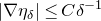 $|\nabla \eta_\delta| \leq C \delta^{-1}$
. Sending
$|\nabla \eta_\delta| \leq C \delta^{-1}$
. Sending $\delta \rightarrow 0$
, we conclude
$\delta \rightarrow 0$
, we conclude
 \begin{equation*}\int_{\hat{X} \setminus E} |\nabla u|^2 d \textrm {vol}_{g_0} = 0.\end{equation*}
We conclude that $|\nabla u| = 0$
on
$|\nabla u| = 0$
on $\hat{X} \setminus E$
, and since
$\hat{X} \setminus E$
, and since $\nabla$
is the Chern connection, this implies
$\nabla$
is the Chern connection, this implies
 \begin{equation*} \bar{\partial} u = 0\end{equation*}
on $\hat{X} \setminus E$
. Since u is bounded, by Hartogs’ theorem we may extend u to all of
$\hat{X} \setminus E$
. Since u is bounded, by Hartogs’ theorem we may extend u to all of $\hat{X}$
. Thus, u is a holomorphic endomorphism of the tangent bundle
$\hat{X}$
. Thus, u is a holomorphic endomorphism of the tangent bundle $T^{1,0} \hat{X}$
. Since
$T^{1,0} \hat{X}$
. Since $\hat{X}$
is a Calabi–Yau threefold with finite fundamental group, we conclude (see (23)) that u must be a multiple of the identity:
$\hat{X}$
is a Calabi–Yau threefold with finite fundamental group, we conclude (see (23)) that u must be a multiple of the identity: $u = \lambda \, \textrm{id}$
. This completes the proof of Lemma 12.
$u = \lambda \, \textrm{id}$
. This completes the proof of Lemma 12.
Appendix B. The (local) map
$\Phi$

We collect several results regarding the map $\Phi: V_0 \setminus \{ 0 \} \rightarrow V_1$
. We recall that
$\Phi: V_0 \setminus \{ 0 \} \rightarrow V_1$
. We recall that $\Phi$
was defined by
$\Phi$
was defined by
 \begin{equation*} \Phi(z) = z + \frac{\overline{z}}{2 \|z\|^2}.\end{equation*}
We will show that $\Phi$
is a diffeomorphism from
$\Phi$
is a diffeomorphism from $\{z \in V_0 \mid \|z\|^2 \gt 1/2 \}$
to
$\{z \in V_0 \mid \|z\|^2 \gt 1/2 \}$
to $\{z \in V_1 \mid \| z \|^2 \gt 1\}$
.
$\{z \in V_1 \mid \| z \|^2 \gt 1\}$
.
We start by taking the norm:
 \begin{equation*} \|\Phi(z)\|^2 = \|z\|^2 \cdot \Big( 1 + \frac{1}{4 \|z\|^4} \Big).\end{equation*}
Let $x = \| z \|^2$
, and remark that the function
$x = \| z \|^2$
, and remark that the function
 \begin{equation*} f(x) = x \Big( 1 + \frac{1}{4x^2} \Big), \quad x \gt 0\end{equation*}
is strictly increasing on $({\tfrac{1}{2}},\infty)$
. From this, we see that
$({\tfrac{1}{2}},\infty)$
. From this, we see that $\Phi$
is injective on
$\Phi$
is injective on $V_0 \setminus \{ \| z \|^2 \leq {\tfrac{1}{2}} \}$
. Indeed, suppose that
$V_0 \setminus \{ \| z \|^2 \leq {\tfrac{1}{2}} \}$
. Indeed, suppose that $\Phi(z) = \Phi(z')$
, with
$\Phi(z) = \Phi(z')$
, with $\| z \|^2\gt {{\tfrac{1}{2}}}$
and
$\| z \|^2\gt {{\tfrac{1}{2}}}$
and $\| z' \|^2 \gt {{\tfrac{1}{2}}}$
. Then the restriction of the domain implies that
$\| z' \|^2 \gt {{\tfrac{1}{2}}}$
. Then the restriction of the domain implies that $\|z\|^2 = \|z'\|^2$
. From here, we can split the equation
$\|z\|^2 = \|z'\|^2$
. From here, we can split the equation $\Phi(z) = \Phi(z')$
into real and imaginary parts and a straightforward calculation shows
$\Phi(z) = \Phi(z')$
into real and imaginary parts and a straightforward calculation shows $z=z'$
.
$z=z'$
.
Our next step is to find an inverse for $\Phi$
. First, we note that
$\Phi$
. First, we note that
 \begin{equation*} g(x) = \tfrac{1}{2} (x + \sqrt{x^2 - 1}), \quad x \gt 1\end{equation*}
is an inverse of $f: ({\tfrac{1}{2}},\infty) \rightarrow (1,\infty)$
.
$f: ({\tfrac{1}{2}},\infty) \rightarrow (1,\infty)$
.
Now, let $w \in V_1$
, with
$w \in V_1$
, with $\|w\|^2 = B \gt 1$
. It can be checked by direct calculation that
$\|w\|^2 = B \gt 1$
. It can be checked by direct calculation that
 \begin{equation*} z_i = \bigg(\frac{2g(B)}{2g(B)+1} \bigg) \cdot \text{{Re}}(w_i) - \sqrt{-1} \cdot \bigg(\frac{2g(B)}{2g(B)-1}\bigg) \cdot \text{{Im}}(w_i)\end{equation*}
satisfies ${\unicode{x2013}}$ $z \in V_0$
;
$z \in V_0$
; ${\unicode{x2013}}$ $\|z\|^2 = g(B) \gt {\tfrac{1}{2}}$
; and
$\|z\|^2 = g(B) \gt {\tfrac{1}{2}}$
; and ${\unicode{x2013}}$ $\Phi(z) = w$
.
$\Phi(z) = w$
.
It follows that $\Phi$
is a bijection from
$\Phi$
is a bijection from $\{z \in V_0 \mid \|z\|^2 \gt {\tfrac{1}{2}}\}$
to
$\{z \in V_0 \mid \|z\|^2 \gt {\tfrac{1}{2}}\}$
to $\{z \in V_1 \mid \|z\|^2 \gt 1 \}$
. The coordinate expressions for
$\{z \in V_1 \mid \|z\|^2 \gt 1 \}$
. The coordinate expressions for $\Phi$
and the ones appearing in the previous computations show that
$\Phi$
and the ones appearing in the previous computations show that $\Phi$
and its inverse are smooth, hence
$\Phi$
and its inverse are smooth, hence $\Phi$
is a diffeomorphism between these sets. Written in terms of
$\Phi$
is a diffeomorphism between these sets. Written in terms of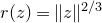 $r(z) = \|z\|^{{{2}/{3}}}$
, we get the following.
$r(z) = \|z\|^{{{2}/{3}}}$
, we get the following.
Proposition 3. The map $\Phi \colon V_0 \setminus \{z \in V_0 \mid r(z) \gt 2^{-{{1}/{3}}}\} \rightarrow \{z \in V_1 \mid r(z) \gt 1 \}$
is a diffeomorphism.
$\Phi \colon V_0 \setminus \{z \in V_0 \mid r(z) \gt 2^{-{{1}/{3}}}\} \rightarrow \{z \in V_1 \mid r(z) \gt 1 \}$
is a diffeomorphism.
We recall that we can compose the map $\Phi$
with scaling maps
$\Phi$
with scaling maps $S_R^*$
. In particular, we defined
$S_R^*$
. In particular, we defined $\Phi_t = S_{t^{{{1}/{3}}}} \circ \Phi \circ S_{t^{-{{1}/{3}}}}$
. One can check that in coordinates, this map takes the form
$\Phi_t = S_{t^{{{1}/{3}}}} \circ \Phi \circ S_{t^{-{{1}/{3}}}}$
. One can check that in coordinates, this map takes the form
 \begin{equation*} \Phi_t(z) = z + \frac{t\overline{z}}{2 \|z\|^2}.\end{equation*}
Smoothness of the scaling maps gives us the following corollary.
Corollary 2. The maps $\Phi_t \colon V_0 \setminus \{z \in V_0 \mid r(z) \gt 2^{-{{1}/{3}}} \cdot t^{{{1}/{3}}} \} \rightarrow \{z \in V_1 \mid r(z) \gt t^{{{1}/{3}}} \}$
are diffeomorphisms for
$\Phi_t \colon V_0 \setminus \{z \in V_0 \mid r(z) \gt 2^{-{{1}/{3}}} \cdot t^{{{1}/{3}}} \} \rightarrow \{z \in V_1 \mid r(z) \gt t^{{{1}/{3}}} \}$
are diffeomorphisms for $t \gt 0$
.
$t \gt 0$
.
Acknowledgements
The authors thank J. Bryan, J. Chen, and A. Fraser for helpful discussions. We also thank the referee for helpful comments and suggestions. SP thanks T.C. Collins and S.-T. Yau for previous collaborations on conifold transitions.
Conflicts of interest
None.
Financial support
This research is supported by an NSERC Discovery Grant.
Journal information
Compositio Mathematica is owned by the Foundation Compositio Mathematica and published by the London Mathematical Society in partnership with Cambridge University Press. All surplus income from the publication of Compositio Mathematica is returned to mathematics and higher education through the charitable activities of the Foundation, the London Mathematical Society and Cambridge University Press.


 Open access

