


Impact statement
This work explores a flexible solution to measure water levels using a network of river cameras. The challenge with river cameras is to automate the extraction of the river water levels, or a related index, from the images. Existing methods only able produce water-level indexes that are not calibrated (relative to the camera field of view), which narrows their range of applications. This work is the first to propose a method that automatically estimates calibrated water-level indexes from images. For this purpose, a dataset of 95 cameras and 32,715 images cross-referenced with gauge data was created. This dataset was used to train deep convolutional neural networks able to extract calibrated river water-level indexes from images.
1. Introduction
Flood events are a recurring natural hazard causing injuries, homelessness, economic losses, and deaths all over the world, every year (Guerreiro et al., Reference Guerreiro, Dawson, Kilsby, Lewis and Ford2018). The severity of floods is even increasing with climate change and growing human activity, such as building assets over land close to river banks (Alfieri et al., Reference Alfieri, Burek, Feyen and Forzieri2015). It is therefore necessary to employ effective and efficient techniques to monitor flood events to avoid economic, social, and human losses. We present a novel deep-learning methodology that takes as input an image coming from a river camera and outputs a corresponding river-level index. The river cameras used as inputs may be different from those used to train the deep-learning model. This research has been performed in order to develop a new flexible tool allowing the observation of flood events.
The current techniques to forecast and manage river flood events are limited by the difficulty of obtaining accurate measurements of rivers.
River gauges provide water levels and calibrated streamflow at point locations and high temporal frequency (e.g., every 15 minutes in England (EA, 2021)). The problem with observing a flood by using gauges is that gauges are expensive to construct and maintain and hence typically sparse. For example, in the UK, gauge stations are typically constructed every 10–60 km (Neal et al., Reference Neal, Schumann, Bates, Buytaert, Matgen and Pappenberger2009). Furthermore, their number is declining globally (Mishra and Coulibaly, Reference Mishra and Coulibaly2009; Global Runoff Data Center, 2016). In addition, gauges can be overwhelmed during flood events (Vetra-Carvalho et al., Reference Vetra-Carvalho, Dance, Mason, Waller, Cooper, Smith and Tabeart2020).
A second approach to obtain river-level information consists in using satellite and aerial images either through expert observation and image processing (e.g., Perks et al., Reference Perks, Russell and Large2016; Mason et al., Reference Mason, Bevington, Dance, Revilla-Romero, Smith, Vetra-Carvalho and Cloke2021; Mauro et al., Reference Mauro, Hostache, Matgen, Pelich, Chini, van Leeuwen, Nichols and Blöschl2021) or through deep learning (e.g., Nemni et al., Reference Nemni, Bullock, Belabbes and Bromley2020). When combined with a digital elevation model (DEM), they can be used to derive water levels along the flood edge (see Grimaldi et al., Reference Grimaldi, Li, Pauwels and Walker2016 for a review). These images can be obtained with optical sensors or synthetic aperture radar (SAR). However, optical techniques are hampered by their daylight-only application and their inability to map flooding beneath clouds and vegetation (Yan et al., Reference Yan, Di Baldassarre, Solomatine and Schumann2015). On the other hand, SAR images are unaffected by clouds and can be obtained day or night. Thus, their relevance for flood mapping in rural areas is well established (e.g., Mason et al., Reference Mason, Schumann, Neal, Garcia-Pintado and Bates2012; Alfieri et al., Reference Alfieri, Burek, Dutra, Krzeminski, Muraro, Thielen and Pappenberger2013; Giustarini et al., Reference Giustarini, Hostache, Kavetski, Chini, Corato, Schlaffer and Matgen2016). In urban areas, shadow and layover issues make the flood mapping more challenging (e.g., Tanguy et al., Reference Tanguy, Chokmani, Bernier, Poulin and Raymond2017; Mason et al., Reference Mason, Dance, Vetra-Carvalho and Cloke2018; Mason et al., Reference Mason, Bevington, Dance, Revilla-Romero, Smith, Vetra-Carvalho and Cloke2021; Mauro et al., Reference Mauro, Hostache, Matgen, Pelich, Chini, van Leeuwen, Nichols and Blöschl2021). In addition, SAR satellite overpasses are infrequent (at most once or twice per day, depending on location), so it is uncommon to capture the rising limb of the flood (Grimaldi et al., Reference Grimaldi, Li, Pauwels and Walker2016), which prevents considering this technique for the live monitoring of floods.
Recently, new solutions have been considered in order to accurately monitor floods, and among them, the use of river cameras has received significant attention (Tauro et al., Reference Tauro, Selker, Van De Giesen, Abrate, Uijlenhoet, Porfiri, Manfreda, Caylor, Moramarco, Benveniste, Ciraolo, Estes, Domeneghetti, Perks, Corbari, Rabiei, Ravazzani, Bogena, Harfouche, Brocca, Maltese, Wickert, Tarpanelli, Good, Alcala, Petroselli, Cudennec, Blume, Hut and Grimaldi2018). River cameras are CCTV cameras (Closed-Circuit TeleVision, video surveillance cameras typically used for monitoring and recording activities), installed with a fixed field of view to observe a river. They provide a continuous stream of images and may be installed by individuals to monitor river water levels for recreational purposes (fishing or boating for example) and are also used by public or private organizations for river monitoring purposes. They are flexible as they can rely on battery supplies and upload images through broadband/4G connections and can be easily installed (e.g., on trees, buildings, or lamp posts). However, a limitation of this approach is the annotation of such images. Indeed, flood case studies have considered floods through manually annotated camera images (e.g., Vetra-Carvalho et al., Reference Vetra-Carvalho, Dance, Mason, Waller, Cooper, Smith and Tabeart2020) but their manual annotation is complex, time-consuming, and requires on-site ground survey. In consequence, it is not possible to straightforwardly repeat this process manually on a large scale, and thus strongly limits the use of river cameras for flood monitoring. There are existing initiatives that rely on crowd-sourcing approaches to share the burden of the annotation process (e.g. Baruch, Reference Baruch2018; Lowry et al., Reference Lowry, Fienen, Hall and Stepenuck2019; Etter et al., Reference Etter, Strobl, van Meerveld and Seibert2020). These processes are made accessible through the help of graphical tools such as virtual gauges, and guidelines to help the annotator perform their annotation task and attribute a flood severity index to an image. However, it has been noted that the crowd-sourced annotations are often inaccurate and their number depends on the degree of investment of the volunteers involved with the project (Etter et al., Reference Etter, Strobl, van Meerveld and Seibert2020).
Several studies have already considered the development of deep learning and computer vision algorithms for flood monitoring via the semantic segmentation of water in images. (Semantic segmentation is a method that classifies pixels according to their content. In this case, we detect whether each pixel contains water or not, e.g., Moy de Vitry et al., Reference Moy de Vitry, Kramer, Wegner and Leitão2019; Vandaele et al., Reference Vandaele, Dance and Ojha2021.) However, on its own, the semantic segmentation of water is of limited interest when it comes to finding the (evolution of the) water level of the river in the image. Indeed, the first way to use the segmentation consists in taking a time series of images of the same camera to observe the relative evolution of the percentage of flooded pixels of (a region of) the image. However, it only allows production of an uncalibrated water-level index, dependent on the field of view of the camera (Moy de Vitry et al., Reference Moy de Vitry, Kramer, Wegner and Leitão2019). The second solution is to carry out ground surveys in order to match the segmented water with the height of surveyed locations within the field of view to estimate the river water level. However, carrying out ground surveys is impractical since spots of interest could be hard or even dangerous to access and field studies would drastically reduce the automation potential of river camera images. A third solution that would consist in merging the camera images with digital elevation models can only be performed manually at this stage, as current literature suggests that deep learning methods are not accurate enough to perform such tasks (Mertan et al., Reference Mertan, Duff and Unal2021). An object detection approach has also been considered to evaluate flood situations in urban areas (Rizk et al., Reference Rizk, Nishimur, Yamaguchi and Higashino2022). However, this methodology relies on the deployment of drones and the presence of specific objects (flooded cars or houses), which limits the potential of the method to capture the rising limb of the flood (before the deployment of the drones and/or before the cars and homes get flooded). Until now, deep learning approaches for river water-level monitoring using images have thus been limited to the production of either uncalibrated river water levels dependent on the field of view of the camera (Moy de Vitry et al., Reference Moy de Vitry, Kramer, Wegner and Leitão2019; Vandaele et al., Reference Vandaele, Dance and Ojha2021), or reliant on field surveys (Vetra-Carvalho et al., Reference Vetra-Carvalho, Dance, Mason, Waller, Cooper, Smith and Tabeart2020). This may be because to our knowledge there is no large dataset of river camera images annotated with river water levels.
In this work, we propose a new approach for extracting calibrated river water-level indexes from river camera images. This approach is able to produce two calibrated indexes: one for continuous river water-level monitoring, and the other boolean for the detection of flood events. This approach is based on the creation of a large dataset of river camera images extracted at 95 camera locations, cross-referenced with river water levels coming from nearby gauges to train deep learning networks. In consequence, we bring the following contributions:
-
• A dataset of images annotated with river water levels, built by cross-referencing river cameras with nearby river water-level measurements produced by gauges.
-
• A deep learning methodology to train two deep convolutional neural networks (CNNs):
-
– Regression-WaterNet, which can provide a continuous and calibrated river water-level index. This network is aimed at providing an index useful for the live monitoring of river water levels.
-
– Classification-WaterNet, which can discriminate river images observing flood situations from images observing unflooded situations. This network is aimed at providing local flood warnings that could enhance existing flood warning services.
-
• An analysis showing that our methodology can be used as a reliable solution to monitor flood events at ungauged locations.
We note that there are uncertainties in the dataset. Firstly, these are due to inaccuracies of gauge measurements (see McMillan et al., Reference McMillan, Krueger and Freer2012 for a complete review). Secondly, uncertainties are introduced by the association of the camera with gauges that are not co-located (see Section 2.1). Nevertheless, our results demonstrate that river cameras and deep learning have a major potential for the critical task of river water-level monitoring in the context of flood events.
The rest of this manuscript is divided into three sections. Section 2 details the methodology used to develop the approach, including the building of the dataset, the definition of the calibrated indexes, and the development and training of the deep learning network that estimated calibrated river water-level indexes. Section 3 presents an analysis of the results obtained by the networks, notably through the comparison with water-level data from distant gauges. Finally, in Section 4, we conclude that our methodology is able to accurately produce two types of calibrated river water-level indexes from images: one for continuous river water-level monitoring, and one for flood event detection. This work is an important step toward the automated use of cameras for flood monitoring.
2. Methodology
As outlined in the introduction, the goal of this work is to create two models. Both take as input an image from a river camera. The aim of the first model is to estimate a continuous index related to the severity of the flood situation within the image. The aim of the second model is to estimate if the location within the image is flooded or not, thus a binary index. The idea is that both models will learn visual cues regarding the presence (or severity) of a flood event within the image such as the color of the water and floating objects. In order to create these models by using supervised deep learning approaches, a dataset where river camera images labeled with such indexes is necessary. This section describes the methodology that was employed for creating such a dataset and the process to develop and train the flood monitoring deep learning models called WaterNets on this dataset. First, Section 2.1 explains the creation process for the large dataset of images where each image is labeled with a river water level. Second, Section 2.2 details the different approaches considered to transform these river water levels into calibrated indexes representing the severity of a flood situation. Finally, Section 2.3 presents the WaterNet CNN architectures that were used to learn the relationships between the images and their river water levels from the dataset.
2.1. Creation of the dataset
This section discusses the preparation of the initial dataset that labels river camera images with river gauge water-level measurements in meters. This was done by associating each river camera with a nearby gauge located on the same river. These measurements are either relative to a local stage datum (Above Stage Datum, mASD), or an ordnance datum (Above Ordnance Datum, mAOD, measured relative to the mean sea level). The transformation of these two types of river water levels into calibrated indexes is presented in Section 2.2.
2.1.1. Acquisition of the river water levels
The various environmental agencies of the United Kingdom and the Republic of Ireland publicly provide data related to the river water levels measured in the gauge stations distributed across their territories: Environment Agency (EA) in England (EA, 2021), Natural Resources Wales (NRW) in Wales (NRW, 2021), Scottish Environment Protection Agency (SEPA) in Scotland (SEPA, 2021), Department for Infrastructure (DfI) in Northern Ireland (DfI, 2021), and Office for Public Works (OPW) in the Republic of Ireland (OPW, 2021). In England, the EA only provides water-level data on an hourly basis for the last 12 months. Consequently, this work only considered the water levels (and images) for the year 2020. For each gauge station, the EA also provides an API allowing the retrieval of the GPS coordinates of the gauges, as well as the name of the river on which they are located. The other agencies allow the retrieval of the GPS locations and rivers monitored through accessible graphical interfaces. In this paper, a gauge, $ g $
, produces pairs
$ g $
, produces pairs $ \left({w}_g,{t}_g\right) $
where
$ \left({w}_g,{t}_g\right) $
where $ {w}_g $
is the water level and
$ {w}_g $
is the water level and $ {t}_g $
is its timestamp. We suppose that there are
$ {t}_g $
is its timestamp. We suppose that there are $ {L}_g $
pairs, ordered by their timestamp. We refer to the ith pair as
$ {L}_g $
pairs, ordered by their timestamp. We refer to the ith pair as $ \left({w}_g(i),{t}_g(i)\right),\hskip0.2em i\in \left[1,2,\dots, {L}_g\right] $
.
$ \left({w}_g(i),{t}_g(i)\right),\hskip0.2em i\in \left[1,2,\dots, {L}_g\right] $
.
2.1.2. Acquisition of the images
We used the network of camera images maintained by Farson Digital WatercamsFootnote
1 for the acquisition of the images. Farson Digital Watercams is a private company that installs cameras on waterways in the UK and the Republic of Ireland. The images from the cameras can be downloaded through an API (subject to an appropriate licensing agreement with the company). At the time of writing this paper, the company had 163 cameras operational. Among these cameras, 104 were installed in England, 9 in the Republic of Ireland, 5 in Northern Ireland, 38 in Scotland, and 7 in Wales. These cameras broadcast one image per hour, between 7 or 8 a.m. and 5 or 6 p.m. (local time). Apart from one camera that was removed from our considerations, the field of view of each camera includes a river, a lake, or the sea. At this stage, they were all kept in the dataset. The images from each camera are available since the installation of the camera, but there can be interruptions due to camera failure or maintenance. After inspection of the cameras, it was observed that a camera may be re-positioned occasionally depending on the wishes of a client, thus changing the field of view at that camera location. Five cameras were moved in 2020. The first cameras were installed in 2009, while the newest were installed in 2020. For each of these cameras, their GPS coordinates and the name of the river/lake/sea in its field of view can be retrieved through Farson Digital’s API. In this paper, a camera, $ c $
, produces pairs
$ c $
, produces pairs $ \left({x}_c,{u}_c\right) $
where
$ \left({x}_c,{u}_c\right) $
where $ {x}_c $
is the image and
$ {x}_c $
is the image and $ {u}_c $
its timestamp. We suppose that there are
$ {u}_c $
its timestamp. We suppose that there are $ {M}_c $
pairs, ordered by their timestamp. We refer to the ith pair as
$ {M}_c $
pairs, ordered by their timestamp. We refer to the ith pair as $ \left({x}_c(i),{u}_c(i)\right),i\in \left[1,2,\dots, {M}_c\right] $
.
$ \left({x}_c(i),{u}_c(i)\right),i\in \left[1,2,\dots, {M}_c\right] $
.
2.1.3. Labeling camera images with river water levels
Each camera was first associated with the closest available gauge on the same river. This was done by computing the Euclidean distance between the gauges and the camera with the GPS coordinates (converted into GNSS) and by matching the river names. These attributes (camera and gauge GPS coordinates and river names) were retrieved using the EA and Farson Digital’s APIs. If the river name was not available for the camera, the association was performed manually using the GPS coordinates and Google Maps. We defined a cut-off distance of 50 km, and cameras that were located more than this distance away from the nearest gauge were removed. The cut-off distance was determined experimentally by making a trade-off between the number of camera images that we could use in the dataset and the proximity of the gauge to the camera. Note that due to a recent cyber-attack on the Scottish agency SEPA Footnote 2, the gauge data monitored by SEPA was not available for this work, which forced us to remove most cameras located in Scotland.
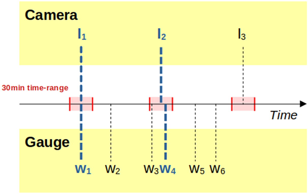
Secondly, the remaining camera images were each labeled with the water-level measurement of the corresponding gauge by matching the timestamp of the image with a timestamp of a water-level recording. The water level that was the closest in time to the image timestamp was chosen, if the measurement was made within a 30-minute time range. If there was no such available water-level measurement, the camera image was discarded. This labeling process between a camera $ c $
and a gauge
$ c $
and a gauge $ g $
is summarised in Figure 1.
$ g $
is summarised in Figure 1.
Example for the association process. A camera has produced images $ {I}_1 $
to
$ {I}_1 $
to $ {I}_3 $
with their timestamps represented by dashed lines projected on the time axis. The acceptable 30 minute time-ranges around the camera timestamps are represented in red. The reference gauge station has produced six water-level measurements
$ {I}_3 $
with their timestamps represented by dashed lines projected on the time axis. The acceptable 30 minute time-ranges around the camera timestamps are represented in red. The reference gauge station has produced six water-level measurements $ {w}_1 $
to
$ {w}_1 $
to $ {w}_6 $
, with their timestamps represented by dashed lines projected on the time axis. The associations are represented in blue. Image
$ {w}_6 $
, with their timestamps represented by dashed lines projected on the time axis. The associations are represented in blue. Image $ {I}_1 $
is associated with gauge level
$ {I}_1 $
is associated with gauge level $ {w}_1 $
as they are produced at the same timestamp. Image
$ {w}_1 $
as they are produced at the same timestamp. Image $ {I}_2 $
has no gauge measurement produced at its timestamp, but both
$ {I}_2 $
has no gauge measurement produced at its timestamp, but both $ {w}_3 $
and
$ {w}_3 $
and $ {w}_4 $
are produced within the 30-minute time range. We choose to associate
$ {w}_4 $
are produced within the 30-minute time range. We choose to associate $ {I}_2 $
with
$ {I}_2 $
with $ {w}_4 $
as it is the closest in time. Image
$ {w}_4 $
as it is the closest in time. Image $ {I}_3 $
has no gauge measurement within the 30-minute time range, so the image will be discarded.
$ {I}_3 $
has no gauge measurement within the 30-minute time range, so the image will be discarded.
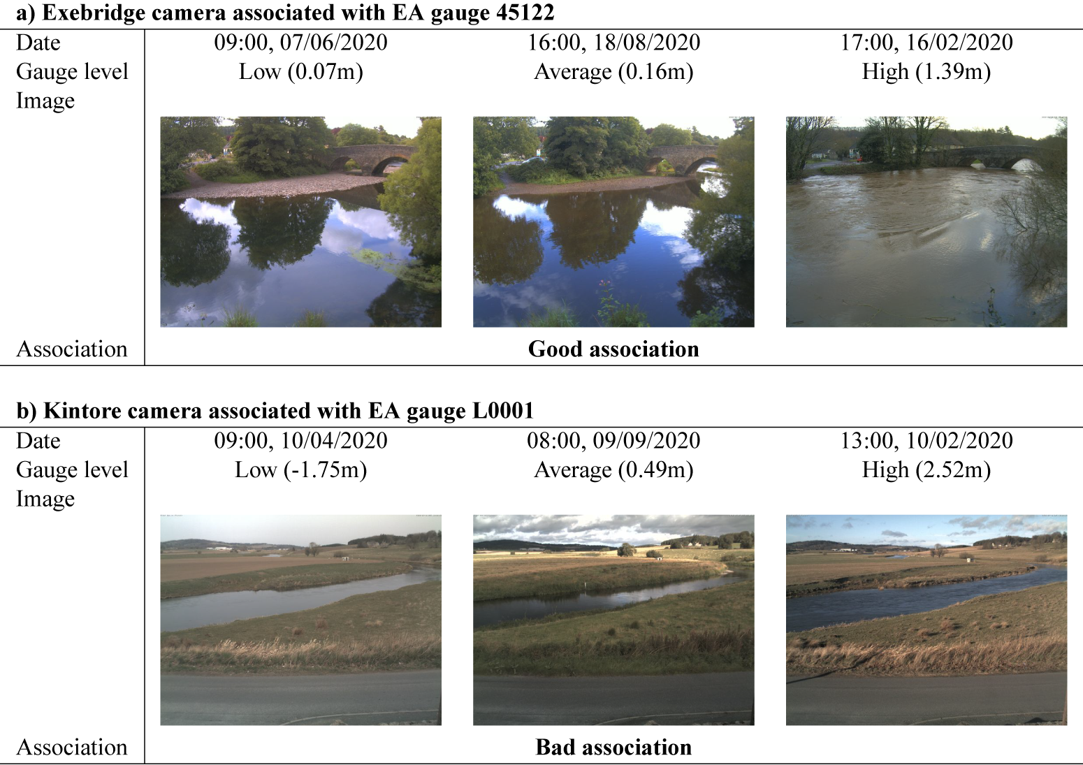
Finally, we performed a visual inspection of the remaining cameras. The idea of this visual inspection process was to remove the bad camera-gauge pairings that were the most obvious. Indeed, several factors such as the river bathymetry, the presence of a lock or a tributary river between the gauge and the camera could have a strong influence on the correlation between the river camera, and the river level measured by its associated gauge station. While lags and other differences between the situation at the gauge and at the camera are unavoidable with our methodology for creating the dataset, we wanted to remove the cameras for which bad pairing was visually obvious in order to avoid training our network on extremely noisy data. The visual inspection process is depicted in Figure 2. For each camera paired with a gauge, three images were selected: the first image had to have been labeled with one of the lowest water levels from the gauge ( $ <5 $
th percentile of all of the water-level heights used to label the camera images). The second image had to have been labeled with a water level that is average for the gauge (within the 45–55th percentile interval of all the gauge measurements). The third image had to have been labeled with one of the highest water levels of the gauge (
$ <5 $
th percentile of all of the water-level heights used to label the camera images). The second image had to have been labeled with a water level that is average for the gauge (within the 45–55th percentile interval of all the gauge measurements). The third image had to have been labeled with one of the highest water levels of the gauge ( $ >95 $
th percentile). The three images were then visually observed side by side to ensure that the river water level visualized in the first image was the smallest, and that the river water level visualized in the third image was the highest. If the camera did not pass this test it meant that the gauge association obviously failed so the camera was discarded from the dataset. Also note that depending on its location, the same gauge can be associated with several river cameras.
$ >95 $
th percentile). The three images were then visually observed side by side to ensure that the river water level visualized in the first image was the smallest, and that the river water level visualized in the third image was the highest. If the camera did not pass this test it meant that the gauge association obviously failed so the camera was discarded from the dataset. Also note that depending on its location, the same gauge can be associated with several river cameras.
Representation of the camera visual inspection process, as explained in Section 2.1. The first camera in Exebridge presented in (a), associated with the EA gauge 45,122 suggests a good association as the image associated with the lowest river water level shows the lowest water level among the three images, and the image associated with the highest river water level shows the highest water level among the three images. The camera in Kintore presented in (b), associated with the EA gauge L0001 suggests a bad association as the image associated with the average water level shows the lowest water level among the three images.
The goal of the visual inspection was to limit the number of bad associations, and thus the noise, in our training set by using an approach that required a reasonable amount of time. Some uncertainties in the quantitative values of the remaining associations still remain. Indeed, as they are not co-located, water-level values at the gauge may not perfectly match the situation at the camera location (due to differences in river bathymetry and local topography, arrival time of a flood wave, etc.). However, gauge data are the only suitable data that are routinely available without making additional measurements in the field. Besides, for the experiments presented in Section 3, these uncertainties are minimized on our test cameras as the quality of the gauge association was inspected during a former study (Vetra-Carvalho et al., Reference Vetra-Carvalho, Dance, Mason, Waller, Cooper, Smith and Tabeart2020). We also compare the quality of our results with all the gauges within a 50 km radius of the test camera (Sections 3.1.2 and 3.2.2). This gives us some understanding of the uncertainty introduced when cameras are not co-located with the river gauge.
In this paper, the labeling process of the data $ \left({x}_c,{u}_c\right) $
from a camera
$ \left({x}_c,{u}_c\right) $
from a camera $ c $
generates triplets
$ c $
generates triplets $ \left({x}_c,{u}_c,{w}_c\right) $
where
$ \left({x}_c,{u}_c,{w}_c\right) $
where $ {x}_c $
is a camera image,
$ {x}_c $
is a camera image, $ {u}_c $
its timestamp, and
$ {u}_c $
its timestamp, and $ {w}_c $
its water-level label. We suppose that there are
$ {w}_c $
its water-level label. We suppose that there are $ {N}_c $
triplets, with
$ {N}_c $
triplets, with $ {N}_c\le {M}_c $
, sorted according to their timestamp. We refer to the ith triplet as
$ {N}_c\le {M}_c $
, sorted according to their timestamp. We refer to the ith triplet as $ \left({x}_c(i),{u}_c(i),{w}_c(i)\right),i\in \left[1,2,\dots, {N}_c\right] $
.
$ \left({x}_c(i),{u}_c(i),{w}_c(i)\right),i\in \left[1,2,\dots, {N}_c\right] $
.
2.1.4. Size of the dataset
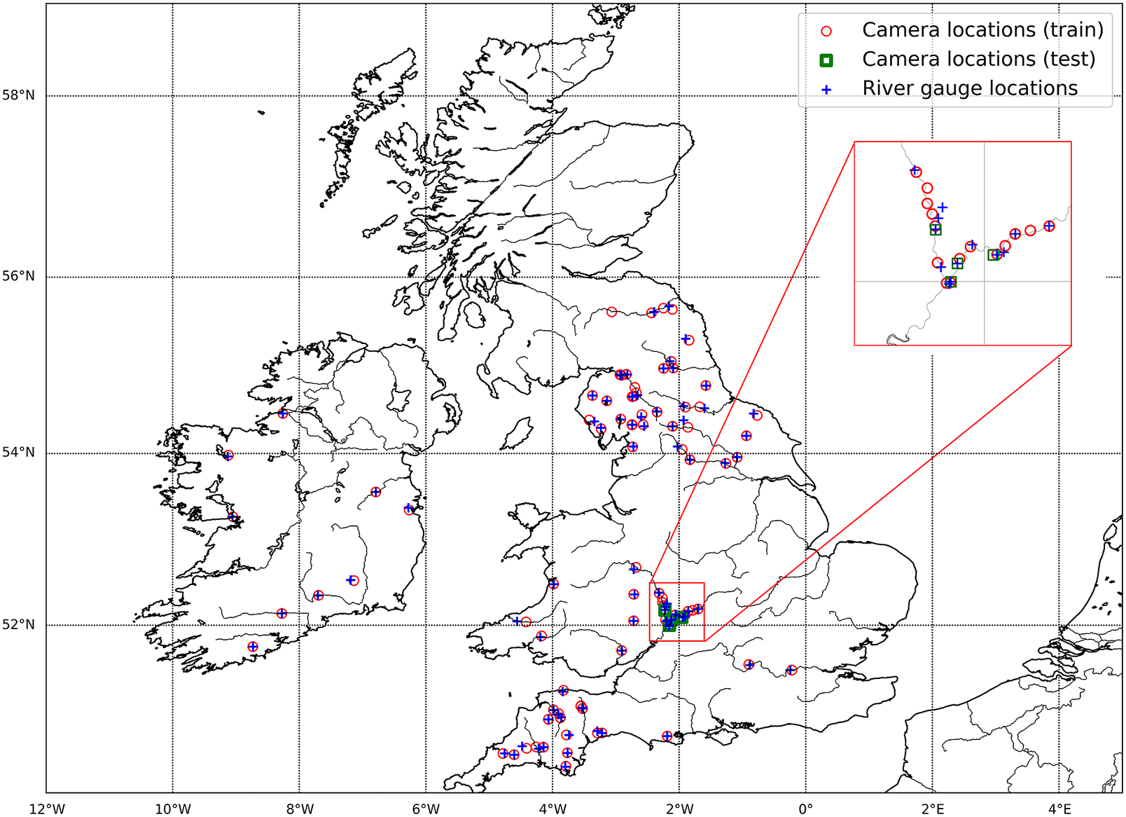
Of the initial 163 cameras, 95 remained after the selection process and were associated with 84 gauges. The number of images per camera is between 583 and 3939 with a median number of 3781 images per camera. The associated gauges are located within a radius of 7 m to 42.1 km, with 50% of these gauges within a radius of 1 km to the camera. A total of 327,215 images of these cameras are labeled with river water levels. Note that this large number of images comes from a limited number of 95 cameras, so there are about 100 different fields of view in the dataset (five cameras in the dataset were moved, so there are more than 95 fields of view). The locations of the selected cameras and their associated gauges are shown in Figure 3.
Locations of the selected cameras and their associated gauges.
2.2. Calibrated flood severity indexes
Section 2.1 discussed the creation of a dataset of images labeled with water levels. The water levels labels are provided in metric units relative to either sea level (mAOD, Above Ordnance Datum) or a stage datum (mASD, Above Stage Datum) chosen according to the local configuration of their gauge station. Without additional topographic information on the site locations, these water levels are thus not calibrated and do not allow observation of river water levels from different cameras in a common reference system. However, a common reference system is necessary for training a model independent of site locations and camera fields of view.
This section outlines the two approaches that were considered in this work in order to calibrate the river water-level measurements obtained from the gauges to allow the observation of the river water level from different cameras in a common reference system.
2.2.1. Standardized river water level
The first approach that was considered was to transform the river water levels $ {w}_g(i) $
into standardized river water levels
$ {w}_g(i) $
into standardized river water levels $ {z}_g(i) $
(z-scores) for each gauge
$ {z}_g(i) $
(z-scores) for each gauge $ g $
independently, subtracting the average water level (for that gauge) from the water level, and then dividing the residual by the standard deviation (for that gauge). This is summarised by the equation
$ g $
independently, subtracting the average water level (for that gauge) from the water level, and then dividing the residual by the standard deviation (for that gauge). This is summarised by the equation
 $$ {z}_g(i)=\frac{w_g(i)-\overline{w_g}}{\sqrt{\frac{1}{L_g}{\sum}_{j=1}^{L_g}{\left({w}_g(j)-\overline{w_g}\right)}^2}}, $$
where $ \overline{w_g}=\frac{1}{L_g}{\sum}_{k=1}^{L_g}{w}_g(k) $
.
$ \overline{w_g}=\frac{1}{L_g}{\sum}_{k=1}^{L_g}{w}_g(k) $
.
With this approach, the gauge river water levels of the cameras are in the same reference system. Indeed, the river water levels of each gauge share a common mean 0 and variance 1. Also note that the reference (sea level or stage datum) has no impact on the definition of this index. This index $ {z}_g(i) $
is thus a continuous metric for the monitoring of river water levels. The higher the index is, the higher the water level is.
$ {z}_g(i) $
is thus a continuous metric for the monitoring of river water levels. The higher the index is, the higher the water level is.
These indexes are computed for each gauge, and then used to label the camera images following the association and labeling process explained in Section 2.1. In this case, this process generates triplets $ \left({x}_c,{u}_c,{z}_c\right) $
. We refer to the ith triplet as
$ \left({x}_c,{u}_c,{z}_c\right) $
. We refer to the ith triplet as $ \left({x}_c(i),{u}_c(i),{z}_c(i)\right),i\in \left[1,2,\dots, {N}_c\right] $
.
$ \left({x}_c(i),{u}_c(i),{z}_c(i)\right),i\in \left[1,2,\dots, {N}_c\right] $
.
2.2.2. Flood classification index
The second approach that was considered was to transform the river water levels produced by a gauge $ g $
with a binary True/False index
$ g $
with a binary True/False index $ {b}_g(i) $
, where
$ {b}_g(i) $
, where $ {b}_g(i) $
represents the flood situation (True if flooded, False otherwise), such that
$ {b}_g(i) $
represents the flood situation (True if flooded, False otherwise), such that
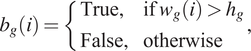 $$ {b}_g(i)=\left\{\begin{array}{ll}\mathrm{True},& \mathrm{if}\;{w}_g(i)>{h}_g\\ {}\mathrm{False},& \mathrm{otherwise}\end{array}\right., $$
where $ {h}_g $
is a threshold specific to the gauge
$ {h}_g $
is a threshold specific to the gauge $ g $
producing the river water-level measurements.
$ g $
producing the river water-level measurements.
According to the EA documentation (EA, 2021), the gauge metadata includes a Typical High water-level threshold set to the 95th percentile of all the water levels measured at that gauge since its installation. This threshold was chosen as the flood threshold $ {h}_g $
in this work as it was available for most of our gauges, and as percentile thresholds are regularly used to evaluate peak discharge (Matthews et al., Reference Matthews, Barnard, Cloke, Dance, Jurlina, Mazzetti and Prudhomme2022). When this threshold was not available as metadata (e.g., gauges in the Republic of Ireland), if a camera was associated with this gauge, it was removed for this specific experiment.
$ {h}_g $
in this work as it was available for most of our gauges, and as percentile thresholds are regularly used to evaluate peak discharge (Matthews et al., Reference Matthews, Barnard, Cloke, Dance, Jurlina, Mazzetti and Prudhomme2022). When this threshold was not available as metadata (e.g., gauges in the Republic of Ireland), if a camera was associated with this gauge, it was removed for this specific experiment.
Similarly to the standardized river water level, these indexes are computed for each gauge, and used to label the camera images following the association and labeling process explained in Section 2.1. In this case, this process generates triplets $ \left({x}_c,{u}_c,{b}_c\right) $
. We refer to the
$ \left({x}_c,{u}_c,{b}_c\right) $
. We refer to the $ i $
th triplet as
$ i $
th triplet as $ \left({x}_c(i),{u}_c(i),{b}_c(i)\right),i\in \left[1,2,\dots, {N}_c\right] $
.
$ \left({x}_c(i),{u}_c(i),{b}_c(i)\right),i\in \left[1,2,\dots, {N}_c\right] $
.
2.3. WaterNet architectures and training
In this work, we rely on a ResNet-50 convolutional neural network. Convolutional Neural Networks are a specific type of neural network.
A neural network is divided into layers of neurons. A neuron computes a linear combination of the output of the neurons of the previous layer (except the first layer which uses the input data). The coefficients used for this linear combination are called weights. In typically supervised learning frameworks where labeled data is available, these weights are found during an optimization procedure that tries to minimize the difference between the output of the network and the true labels of the data according to a given loss function.
As we noted in Vandaele et al. (Reference Vandaele, Dance and Ojha2021), “A convolutional neural network contains a specific type of layers with specific types of neurons, designed to take into account the spatial relationships between values of a two-dimensional structure, such as an image. The neurons of a convolutional layer can be seen as filters (matrices) of size $ F\times F\times {C}_i $
, where
$ F\times F\times {C}_i $
, where $ {C}_i $
is the number of channels of the input (e.g., 3 for a RGB image) at layer
$ {C}_i $
is the number of channels of the input (e.g., 3 for a RGB image) at layer $ i $
. The input is divided into square sub-regions (tiles) of size
$ i $
. The input is divided into square sub-regions (tiles) of size $ F\times F\times {C}_i $
that can possibly overlap. Each neuron/filter of the convolutional layer is applied on each of the tiles of the image by computing the sum of the Hadamard product (element-wise matrix multiplication). If organized spatially, the output of a convolutional layer can be seen as another image which itself can be processed by another convolutional layer: if a convolutional layer is composed of
$ F\times F\times {C}_i $
that can possibly overlap. Each neuron/filter of the convolutional layer is applied on each of the tiles of the image by computing the sum of the Hadamard product (element-wise matrix multiplication). If organized spatially, the output of a convolutional layer can be seen as another image which itself can be processed by another convolutional layer: if a convolutional layer is composed of $ N $
filters, then the output image of this convolutional layer has
$ N $
filters, then the output image of this convolutional layer has $ N $
channels.”
$ N $
channels.”
CNN architectures vary in a number of layers and choice of activation function, but also in terms of additional layers such as nonconvolutional layers at the end of the network. ResNet-50 is the architecture of the convolutional neural network (He et al., Reference He, Zhang, Ren and Sun2016). This architecture has reached state-of-the-art performance in image classification tasks (He et al., Reference He, Zhang, Ren and Sun2016). Besides, its implementation is easily available in various deep-learning libraries, such as PyTorch (Paszke et al., Reference Paszke, Gross, Massa, Lerer, Bradbury, Chanan, Killeen, Lin, Gimelshein, Antiga, Desmaison, Kopf, Yang, DeVito, Raison, Tejani, Chilamkurthy, Steiner, Fang, Bai and Chintala2019).
Similarly to our previous work (Vandaele et al., Reference Vandaele, Dance and Ojha2021), we modified the last layer of this architecture in order to match our needs: indeed, the last layer of this architecture is a layer of 1,000 neurons to provide 1,000 values for the ImageNet classification task (Deng et al., Reference Deng, Dong, Socher, Li, Li and Fei-Fei2009). Thus, as we consider the estimation of two different river water-level indexes, we defined two corresponding network architectures for which the only difference with ResNet-50 is the last layer:
-
• For the Standardized river water-level index (see Section 2.2.1), the last layer of ResNet-50 was changed to a one-neuron layer. We will refer to this network as Regression-WaterNet.
-
• For the Flood classification index (see Section 2.2.2), the last layer of ResNet-50 was changed to a two-neuron layer with the last layer being a SoftMax layer. We will refer to this network as Classification-WaterNet.
In order to train the networks, we chose to rely on a transfer learning approach which has already proven useful to improve the performance of water segmentation networks (Vandaele et al., Reference Vandaele, Dance and Ojha2021): before training the WaterNet networks over the labeled camera images, all the weights used in the convolution layers, except the last layer, were first set to the values obtained by training the network over the standard large dataset for image classification, ImageNet (Deng et al., Reference Deng, Dong, Socher, Li, Li and Fei-Fei2009). They were then fine-tuned over the labeled camera image dataset. With this transfer methodology, the initial setting of the convolutional layers weights is already efficient at processing image inputs as it was trained over a large multipurpose dataset of RGB images. Thus, it facilitates the training of the network for a new image-processing task.
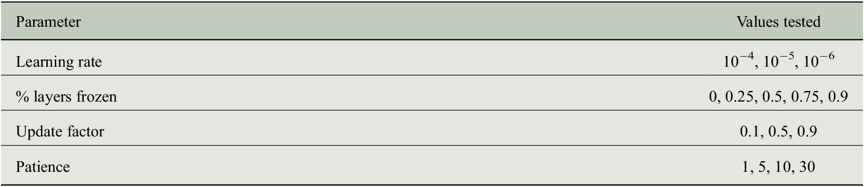
For both Regression-WaterNet and Classification-WaterNet, a grid search was performed to find the optimal learning parameters for training the networks (learning rate, percentage of network layers frozen to the values of the network trained over ImageNet Deng et al., Reference Deng, Dong, Socher, Li, Li and Fei-Fei2009, update factor, patience). The values tested are shown in Table 1. The networks were fine-tuned on the training set over 30 epochs. An L1 loss was used for Regression-WaterNet and a binary cross-entropy loss was used for Classification-WaterNet (Zhang et al., Reference Zhang, Lipton, Li and Smola2021). At each epoch, the network was evaluated on a validation set and the learning rate updated with an update factor if it was not improving for a number of epochs (patience). The weights of the WaterNet network trained with the learning parameters obtaining the best results on the validation set during the grid search were then used to evaluate the performance of the networks on the test set.
Learning parameters tested during the grid search.
3. Experiments
This section describes the results of the experiments that were performed to assess the performance of the WaterNet networks. Two experiments were performed: the first, detailed in Section 3.1, was performed to assess the performance of Regression-WaterNet to estimate the standardized river water-level index. The second experiment, detailed in Section 3.2, assesses the performance of Classification-WaterNet for the estimation of the flood classification index.
3.1. Standardized river water-level index results using Regression-WaterNet
3.1.1. Experimental design
3.1.1.1. Dataset split
As presented in Section 2.1, the dataset at our disposal consisted of 95 cameras. This dataset was divided into three parts:
-
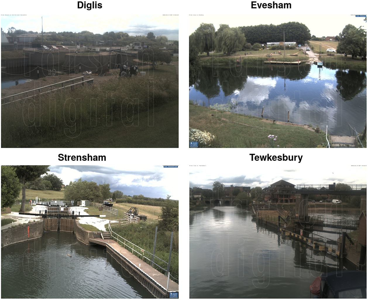
• The test set consisted of the 15,107 images of four cameras that were chosen as these cameras have been previously studied by a human observer and their correspondence to nearby gauge-based water-level observations has been assessed (Vetra-Carvalho et al., Reference Vetra-Carvalho, Dance, Mason, Waller, Cooper, Smith and Tabeart2020): Diglis Lock (abbreviated to Diglis), Evesham, Strensham Lock (abbreviated to Strensham) and Tewkesbury Marina (abbreviated to Tewkesbury). As shown in Figure 4, these four cameras offer four different site configurations. Their associated gauges were respectively located at 58 m, 1.08 km, 37 m, and 53 m from the cameras.
-
• The validation set consisted of 18,894 images from five other cameras that were chosen randomly. We chose to rely on a relatively small sized validation set to keep a large number of different camera fields of view in the training set.
-
• The training set consisted of 293,214 images from the 86 remaining cameras and their images.
Sample images from the four cameras of the test set.
Note that the gauges associated with the cameras of the test set were not associated with cameras of the training and validation set. For this experiment, the images $ {x}_c $
are labeled with the standardized river water-level indexes
$ {x}_c $
are labeled with the standardized river water-level indexes $ {z}_c $
detailed in Section 2.2.1.
$ {z}_c $
detailed in Section 2.2.1.
3.1.1.2. Evaluation protocol
In order to evaluate the efficiency of Regression-WaterNet, we report an error score that consists of the average of the absolute differences (also known as MAE, mean absolute error) between the standardized water-level indexes $ {z}_c(i) $
of the image and the estimation of this standardized water-level index
$ {z}_c(i) $
of the image and the estimation of this standardized water-level index $ {\hat{z}}_c(i) $
over each of the
$ {\hat{z}}_c(i) $
over each of the $ {N}_c $
labeled images from the camera
$ {N}_c $
labeled images from the camera $ c $
using Regression-WaterNet such as
$ c $
using Regression-WaterNet such as
 $$ {\mathrm{MAE}}_c=\frac{1}{N_c}\sum \limits_{i=1}^{N_c}\mid {z}_c(i)-{\hat{z}}_c(i)\mid $$
We propose a novel automated method that outputs calibrated river water-level indexes from river camera images. It is thus not possible to compare our approach to other automated algorithms. However, it is possible to evaluate how well our methodology is working compared to using distant gauges in order to estimate the standardized river water level at a given ungauged location. This evaluation is performed using the following protocol:
-
1. Each test camera is associated with:
-
• A reference gauge is the gauge used to label the images of the camera with water levels, following the protocol described in Section 2.1. In the scope of our experiments, these gauges thus provide the ground-truth water levels at the test camera locations. Note that the quality of the association between the four test cameras and their corresponding reference gauge was assessed in a former study (Vetra-Carvalho et al., Reference Vetra-Carvalho, Dance, Mason, Waller, Cooper, Smith and Tabeart2020).
-
• The other gauges available within a 50 km radius from its location. In the scope of our experiments, these are the distant gauges: they could be used to estimate the standardized river water-level index at the camera location if a reference gauge was not available.
-
-
2. We evaluate the accuracy of using a distant gauge to estimate the standardized river water level at the camera location by comparing the standardized water levels of the distant gauge with the standardized water levels of the reference gauge.
-
• The standardized water levels of the distant and reference gauge are first matched according to their timestamp following a similar procedure than the image labeling procedure described in Section 2.1.
-
• The Mean Absolute Error (see Eq. 3) is computed between the associated standardized water-level indexes.
-
-
3. The Mean Absolute Error obtained by each distant gauge can then be compared with the Mean Absolute Error obtained by our camera-based methodology.
3.1.1.3. Processing the network outputs
After its training following the protocol described in Section 2.3, Regression-WaterNet is able to estimate river water-level indexes from camera images. As the test cameras produce one image every hour (during daylight), the network generates a time series of estimations that can potentially be post-processed. Two approaches were considered to post-process the time series of estimations.
-
• RWN, where the time-series estimations of the Regression-WaterNet network $ {\hat{z}}_c(i) $
for each image
$ {x}_c(i) $
are not post-processed and are thus considered independently. This is representative of cases where the goal would be to obtain independent measurements from single images.
$ {\hat{z}}_c(i) $
for each image
$ {x}_c(i) $
are not post-processed and are thus considered independently. This is representative of cases where the goal would be to obtain independent measurements from single images. -
• Filtered-RWN, where the time series estimations of the Regression-WaterNet network
$ {\hat{z}}_c(i) $
for each image
$ {x}_c(i) $
are replaced by the median
$ {\hat{z}}_c^F(i) $
of the estimations obtained from Regression-WaterNet on all the images available within a 10-hour time window such that


 $$ {\hat{z}}_c^F(i)=\mathrm{median}\hskip0.1em \left(\left\{{\hat{z}}_c(j),|{u}_c(j)-{u}_c(i)|\le 10\hskip0.22em \mathrm{hours}\hskip0.1em \right\}\right), $$
where, as explained in Section 2.1, $ {u}_c(i) $
corresponds to the timestamp of image
$ {u}_c(i) $
corresponds to the timestamp of image $ {x}_c(i) $
. As the images are captured between 8 am and 6 pm, we chose this 10-hour time-window threshold so that the median would apply to all the images captured in the daylight hours of the same day. Filtered-RWN can thus be seen as a post-processing step used to regularize the output of RWN.
$ {x}_c(i) $
. As the images are captured between 8 am and 6 pm, we chose this 10-hour time-window threshold so that the median would apply to all the images captured in the daylight hours of the same day. Filtered-RWN can thus be seen as a post-processing step used to regularize the output of RWN.
3.1.2. Results and discussion
The comparison between the MAE obtained by the distant gauges and our methodology is given in Figure 5. Overall, this figure shows that RWN and Filtered-RWN each allow the monitoring of the river water level from the test cameras as accurately as a gauge within a 50 km radius of the river camera. Indeed, at Strensham and Tewkesbury, the MAE of RWN is similar to the lowest MAE among the gauges that were not associated with the cameras. At Diglis and Evesham, the MAE of RWN and lies in the range between the lowest and highest MAE of the gauges not associated with the camera. The filtering process of Filtered-RWN decreases the error at each location. While there is always a gauge within 50 km that is able to obtain results at least as accurate as RWN, the closest gauge (after the reference gauge) does not always provide the best performance (never, in this case).
MAE scores obtained by applying RWN (dashed line) and Filtered-RWN (dotted line) on the camera images of Diglis, Evesham, Strensham, and Tewkesbury. The bars represent the MAE scores obtained with the standardized river water-level indexes produced by the gauges within a 50 km radius, as described in Section 3.1.1.
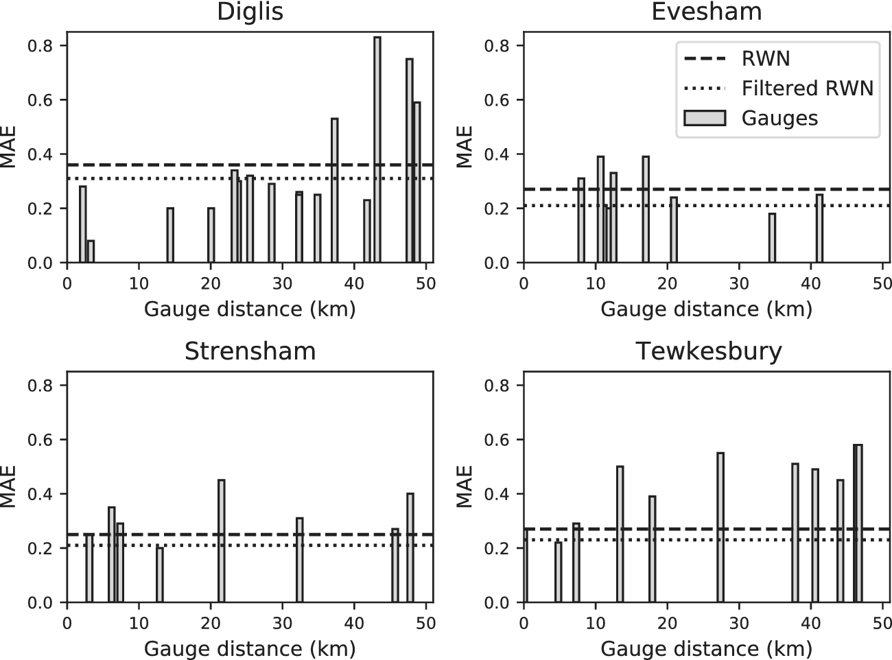
In practice, given an ungauged location in need of river water-level monitoring, it is thus easier to rely on our camera-based methodology than relying on the estimations made by a distant gauge. Indeed, using a distant gauge providing accurate measurements for the ungauged location would require validation data, which is impossible by definition. In consequence, applying RWN or Filtered-RWN on camera images is the most suitable choice.
Figure 6 shows the time series of the standardized index through the year estimated by RWN and Filtered-RWN, compared with gauge data from the reference gauges of the test cameras. RWN brings a significant variability in the observations, but overall the networks are able to successfully observe the flood events (that occur in January, February, March, and December) as well as the lower river level period between April and August. As expected, the median filter used with Filtered-RWN reduces the variability of the image-derived observations, but also tends to underestimate the height of river water levels, especially during high flow and flood events. Filtered-RWN estimates an oscillation of the standardized water level at low water levels at Diglis from March to July that is not explained by the gauge data nor by our visual inspection, and thus corresponds to estimation errors of the network.
Monitoring of the river water levels during 2020 at Diglis, Evesham, Strensham, and Tewkesbury by applying RWN and Filtered-RWN to the camera images, compared to the river water-level data produced by the gauge associated with the camera.

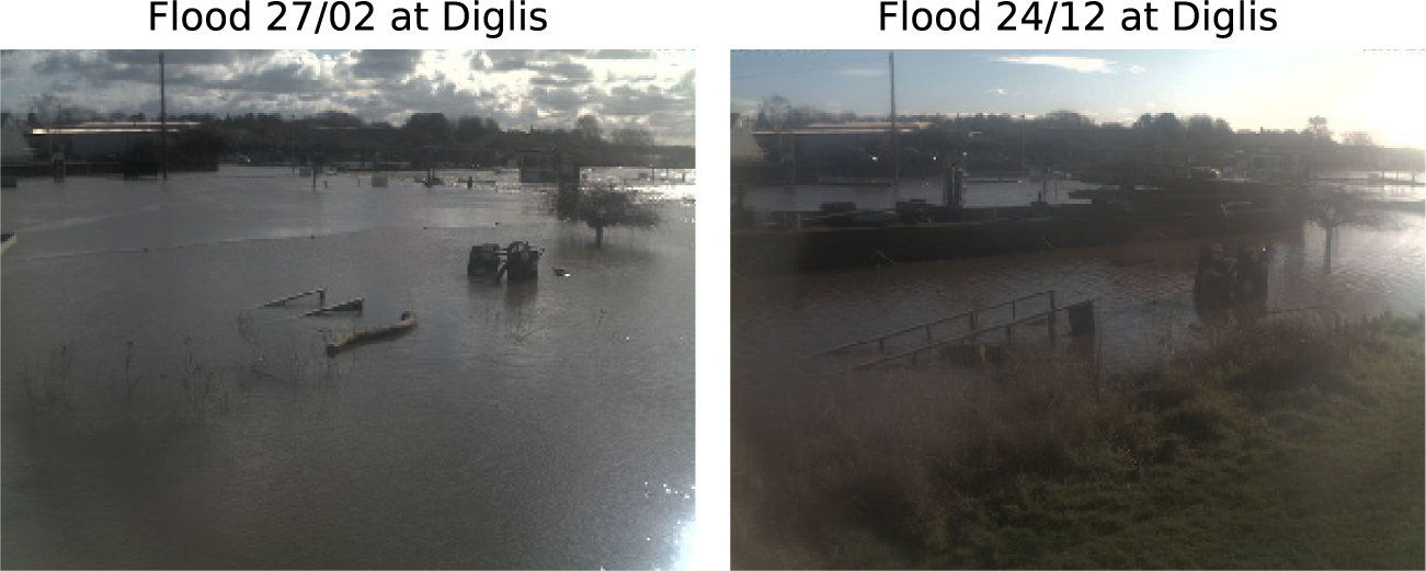
After visual inspection, it was observed that the gauge measurements used to label camera images do not always perfectly match the situation at the camera location, so RWN sometimes gives a better representation of the situation than the standardized river water levels of the gauges. For example, the gauge line in the Diglis plot in Figure 6 suggests that the February and December floods in Diglis have reached the same level, while Filtered-RWN suggests that the December event was smaller than the March event. As suggested by Figure 7, the largest flood extent observed in December at Diglis (24 December) does not reach the height of the largest flood extent observed in February (27 February). Another visible example is the significant sudden water-level drop at the Strensham gauge at the end of April, which is not visible in our image data. This is likely due to a gauge anomaly.
Camera images observing the flood event at Diglis, on 27 February 2020 (left), and on 24 December 2020 (right).
It can thus be concluded that the application of RWN and Filtered-RWN on river camera images allows us to obtain results with similar accuracy to using water-level information from a gauge within a 50 km radius.
3.2. Flood classification index results using Classification-WaterNet
3.2.1. Experimental design
The experimental design used for this experiment is similar to the one used in the first experiment, described in Section 3.1.1. The same cameras were used for the training, validation, and test splits. The images $ {x}_c $
were labeled with the binary flood indexes
$ {x}_c $
were labeled with the binary flood indexes $ {b}_c $
detailed in Section 2.2.2. As explained in Section 2.2.2, the water-level threshold that is considered for the separation between flooded and unflooded situations is defined as the 95th percentile of the water-level heights measured at the gauge since it was installed. This threshold value is obtained as metadata (the “typical high range” variable) alongside the water-level measurements from most EA gauges. Cameras for which we could not retrieve this threshold value were removed for this experiment (13 cameras belonging to the training set).
$ {b}_c $
detailed in Section 2.2.2. As explained in Section 2.2.2, the water-level threshold that is considered for the separation between flooded and unflooded situations is defined as the 95th percentile of the water-level heights measured at the gauge since it was installed. This threshold value is obtained as metadata (the “typical high range” variable) alongside the water-level measurements from most EA gauges. Cameras for which we could not retrieve this threshold value were removed for this experiment (13 cameras belonging to the training set).
Given the definition of the typical high-range threshold, there is a small number of images considered as flooded, which makes the training set imbalanced. The training of Classification-WaterNet was performed using a data augmentation technique that consisted in increasing the number of flooded images by using the same flooded images several times (randomly flipped on their vertical axis) so that 50% of the images used in training were flooded situations.
Similarly to the protocol of the first experiment described in Section 3.1.1, we post-processed the time-series estimations of Classification-WaterNet through two approaches:
-
• CWN, where the time-series estimations of the Classification-WaterNet network
$ {\hat{b}}_c(i) $
for each image
$ {x}_c(i) $
are not post-processed and thus considered independently. This is representative of cases where the goal would be to obtain independent measurements from single pictures. -
• Filtered-CWN outputs the estimated flood classification index
$ {\hat{b}}_c^F(i) $
. In order to create this estimation, the output
$ {\hat{b}}_c(i) $
of CWN is post-processed for each hour by replacing the independent estimation by the most represented class of estimations (flooded/not flooded) obtained within a 10 hour time window. Filtered-CWN can thus be seen as a post-processing step used to regularize the output of CWN.


The following Balanced Accuracy criterion was used to evaluate the performance of the network:
 $$ \hskip0.1em \mathrm{Balanced}\ \mathrm{Accuracy}=0.5\times \frac{\hskip0.1em \mathrm{TP}\hskip0.1em }{\hskip0.1em \mathrm{TP}+\mathrm{FP}\hskip0.1em }+0.5\times \frac{\hskip0.1em \mathrm{TN}\hskip0.1em }{\hskip0.1em \mathrm{TN}+\mathrm{FN}\hskip0.1em }, $$
where
 $$ {\displaystyle \begin{array}{l}\mathrm{TP}=\#\left\{i|{b}_c(i)=\mathrm{True},{\hat{b}}_c(i)=\mathrm{True}\right\},\\ {}\mathrm{FP}=\#\left\{i|{b}_c(i)=\mathrm{False},{\hat{b}}_c(i)=\mathrm{True}\right\},\\ {}\mathrm{TN}=\#\left\{i|{b}_c(i)=\mathrm{False},{\hat{b}}_c(i)=\mathrm{False}\right\},\\ {}\mathrm{FN}=\#\left\{i|{b}_c(i)=\mathrm{False},{\hat{b}}_c(i)=\mathrm{True}\right\},\end{array}} $$
where TP corresponds to the number ( $ \# $
) of correctly classified flooded images, (true positives), FP to the number of incorrectly classified unflooded images (false positives), TN to the number of correctly classified unflooded images (true negatives), and FN to the number of incorrectly classified flooded images (false negatives).
$ \# $
) of correctly classified flooded images, (true positives), FP to the number of incorrectly classified unflooded images (false positives), TN to the number of correctly classified unflooded images (true negatives), and FN to the number of incorrectly classified flooded images (false negatives).
The Balanced Accuracy criterion gives a proportionate representation of the performance of Classification-WaterNet regarding the classification of flooded and unflooded images on the test set. Unlike the training set, the test set was not artificially augmented to contain a proportionate number of flooded and unflooded images.
Similarly to the first experiment (see Section 3.1.1), the performance of the network was also compared with an approach based on the flood classification indexes produced by nearby gauges (within a 50 km radius), located on the same river. Given a reference gauge $ {g}_1 $
and another gauge
$ {g}_1 $
and another gauge $ {g}_2 $
,
$ {g}_2 $
,
 $$ {\displaystyle \begin{array}{l}\mathrm{TP}=\#\left\{\left(i,j\right)|{b}_{g_1}(i)=\mathrm{True},{\hat{b}}_{g_2}(j)=\mathrm{True},{t}_{g_1}={t}_{g_2}\right\},\\ {}\mathrm{FP}=\#\left\{\left(i,j\right)|{b}_{g_1}(i)=\mathrm{False},{\hat{b}}_{g_2}(j)=\mathrm{True},{t}_{g_1}={t}_{g_2}\right\},\\ {}\mathrm{TN}=\#\left\{\left(i,j\right)|{b}_{g_1}(i)=\mathrm{False},{\hat{b}}_{g_2}(j)=\mathrm{False},{t}_{g_1}={t}_{g_2}\right\},\\ {}\mathrm{FN}=\#\left\{\left(i,j\right)|{b}_{g_1}(i)=\mathrm{True},{\hat{b}}_{g_2}(j)=\mathrm{False},{t}_{g_1}={t}_{g_2}\right\},\end{array}} $$
where in this case $ {g}_1 $
is the reference gauge attached to the camera. The Balanced Accuracy between the two gauges can then be computed with Eq. (5).
$ {g}_1 $
is the reference gauge attached to the camera. The Balanced Accuracy between the two gauges can then be computed with Eq. (5).
3.2.2. Results and discussion
Figure 8 compares the Balanced Accuracy scores obtained by CWN and Filtered-CWN with the scores obtained by the nearby gauges producing the flood classification indexes. CWN obtains performance similar to the gauges with the highest Balanced Accuracy score at Strensham, as does Filtered-CWN at Evesham and Tewkesbury. At Diglis, CWN and Filtered-CWN scores are average: they are significantly lower than the highest gauge-based Balanced Accuracy scores, but also significantly higher than the lowest ones.
Balanced Accuracy scores obtained by applying CWN (dashed line) and Filtered-CWN (dotted line) on the camera images of Diglis, Evesham, Strensham, and Tewkesbury. The bars represent the Balanced Accuracy scores obtained by the gauges within a 50 km radius producing a flood classification index, as described in Section 3.2.1.

By looking more closely at the results with the contingency table presented in Table 2, we can make two additional observations.
Contingency table for the classification of flooded images using CWN.
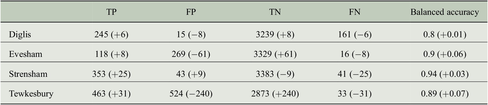
Note. See Section 3.2.1 for the description of TP, FP, TN, and FN. The changes brought with Filtered-CWN are shown between the parentheses.
The first is that Filtered-CWN improves the Balanced Accuracy scores at each of the four locations compared to CWN. Filtered-CWN has a positive impact on the correction of both false positives and false negatives, except at Strensham where it slightly increased the number of false positives.
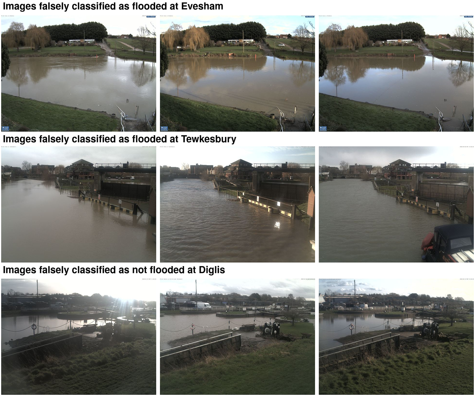
The second is that the networks have a slight tendency to classify unflooded images as flooded at Evesham and Tewkesbury, and flooded images as not flooded at Diglis. However, from our visual analysis of the misclassified examples (see Figure 9 for some examples), many of the images that the network falsely estimated as flooded in Evesham and Tewkesbury are images where the water level is high and close to a flood situation, or seems to be actually flooded. The images wrongly estimated as not flooded at Diglis mostly represent situations where the river is still on the bank. From this analysis, it thus seems that the network is prone to confusing borderline events where the river water level is high but not necessarily high enough to produce a flood event. This can be explained by the fact that the high flow threshold used in this work to separate flooded images from unflooded ones is arbitrary and does not technically separate flooded images (when the river gets out-of-bank) from unflooded ones. Besides, whether the threshold value is statistically representative of the local water-level distribution depends on the number and quality of river water-level records available at the corresponding gauge station. The use of this high flow threshold thus brings uncertainties at borderline flood events (small flood situations or high water levels when the river is not overflowing). However, this visual analysis also showed that our network was able to rightly distinguish obvious large flood events from situations with typical in-bank river water levels.
Examples of images misclassified by Classification-WaterNet.
4. Conclusions
River gauges provide frequent river water-level measurements (e.g., every 15 min in the UK (EA, 2021)), but they are sparsely located and their number is declining globally (Mishra and Coulibaly, Reference Mishra and Coulibaly2009; Global Runoff Data Center, 2016). Satellite images can provide water-level measurements over a wide area when the river is out-of-bank, but are infrequent in time as they rely on satellite overpasses. We investigate the potential of a new source of river water-level data offering a new trade-off between spatial and temporal coverage: river cameras. River cameras are CCTV cameras installed to observe a river. They are cheap and relatively easy to install when compared to gauges, and they produce a live stream of images that could be used for river-level monitoring. However, the CCTV images need to be transformed into quantitative river water-level data by an automated algorithm for this approach to become realistic. This is why this work focused on the development of deep learning-based methods able to estimate calibrated river water levels based on camera images.
With the first part of this work, we have created a dataset of river camera images where each camera was associated with its closest river gauge measuring river water levels. This dataset consists of 32,715 images coming from 95 different cameras across the UK and Ireland labeled with a river water-level value.
In the second part of this work, we used this dataset to train two deep convolutional neural networks. The first one, Regression-WaterNet, estimates standardized river water-level indexes from the images. The second one, Classification-WaterNet, detects flood situations from the images. We were able to show that both networks were a reliable and convenient solution compared to using distant river gauges in order to perform the same river water-level monitoring tasks. Indeed, this solution provides river water-level index estimations as accurate as nearby gauges can provide. We also noticed that the performance of these methods might be better than the numerical evaluation of scores might indicate. Indeed, for both networks, we noticed after a visual inspection that some estimations considered by our numerical evaluation protocol were in fact more representative than the gauge measurements attached to the image.
The promising results of this study demonstrated the potential of deep learning methods on river cameras in order to monitor river water levels, and more specifically floods. This represents a flexible, cost-effective, and accurate alternative to more conventional means to monitor water levels and floods in real-time and has the potential to help in the prevention of further economic, social, and personal losses.
Acknowledgments
The authors would like to thank Glyn Howells from Farson Digital Ltd for granting access to camera images. The authors would also like to thank David Mason, University of Reading, for the useful discussions.
Author contribution
Conceptualization: R.V.; Data curation: R.V.; Data visualization: R.V.; Funding acquisition: S.L.D.; Methodology: R.V.; Project administration: S.L.D.; Supervision: S.L.D., V.O. Writing original draft: R.V.; Writing review and edition: S.L.D., V.O. All authors approved the final submitted draft.
Competing interest
The authors declare none.
Data availability statement
The images used in this work are property of Farson Digital Watercams and can be downloaded on their website https://www.farsondigitalwatercams.com/ subject to licensing conditions. The river gauge data can be found on the websites of the responsible authorities (DfI, 2021; EA, 2021; NRW, 2021; OPW, 2021; SEPA, 2021).
Ethics statement
The research meets all ethical guidelines, including adherence to the legal requirements of the study country.
Funding statement
This research was supported in part by grants from the EPSRC(EP/P002331/1) and the NERC National Center for Earth Observation (NCEO).


 Open access