2.1. Flow conditions

The numerical study performed in this work is based on experiments conducted in the DLR High Enthalpy Shock Tunnel Göttingen, HEG (Wagner Reference Wagner2014; Deutsches Zentrum für Luft - und Raumfahrt -DLR 2018; Wagner et al. Reference Wagner, Wartemann, Dittert and Kütemeyer2019). The present configuration is a hypersonic boundary layer over a 7-degree half-angle cone, and test conditions of $Re_m = 4.1 \times 10^6\ \mathrm {m}^{-1}$ and $Re_m = 6.4 \times 10^6\ \mathrm {m}^{-1}$ are chosen. In table 1, $Re_{m}\equiv \rho _{\infty } u_{\infty }/\mu _{\infty }$ is the Reynolds number per metre, $p$ is pressure, $T$ is temperature, $\rho$ is density, $u$ is velocity and $M$ is Mach number. The subscript $\infty$ indicates free-stream conditions. The wall temperature $T_w$ is $300$ K for all cases, and it is consistent with the experiment because of the short duration of the test run. The $T_w/T_r$ is wall-to-recovery temperature ratio, where $T_r$ is defined as

(2.1)\begin{equation} T_r \equiv T_{\infty} \left(1+r_{turb}\frac{\gamma - 1}{2} M_{\infty}^2 \right), \end{equation}

where $\gamma$ is the specific heat ratio ($\gamma = 1.4$). The parameter $r_{turb}$ is a recovery factor for turbulent boundary layers and it can be approximated as $r_{turb} \approx Pr^{1/3}$ (Dorrance Reference Dorrance1962; White Reference White2006), where $Pr$ is the Prandtl number ($Pr = 0.707$). Since the free-stream temperature is high, the wall-to-recovery temperature ratio decreases to approximately 0.1. Figure 1 provides a sketch of the present configuration. In the experiment, a conical shock is attached to the tip of the cone, and a boundary layer is formed on the cone surface only under the shock. The laminar boundary layer starts from the tip and the transition to turbulence happens further downstream on the surface. In this study, the turbulent region under the shock is simulated with the two Reynolds numbers (M7.4-R4.1 and M7.4-R6.4) using our proposed volumetric rescaling method described in § 2.3. A simulation including the laminar-to-turbulent transition with $Re_m = 4.1 \times 10^6\ \mathrm {m}^{-1}$ (M7.4-LT4.1) is used as reference data. This case has been simulated in previous work by the same authors (Sousa et al. Reference Sousa, Wartemann, Wagner and Scalo2024). In the present simulation, the computational domain is wider in the azimuthal direction, and the mesh is finer in the wall-normal direction. These computational cases are summarized in table 1.

Table 1. List of computational cases and conditions. All symbols are defined in the text.

Figure 1. Sketch of the present conical hypersonic boundary-layer configuration.

2.2. Flow set-up

A precursor axisymmetric RANS simulation is carried out for the present rescaling simulations. The inlet of the RANS computational domain is located in the $x=0.045$ m plane, where $x$ is the distance from the cone tip along the wall surface. The domain length in streamwise direction $L_x$ extends 1 m. The domain height in the wall-normal direction $L_y$ is 0.0022 m at the inlet and 0.05 m at the outlet. These lengths are decided so that the upper domain boundary stays under the shock. The azimuthal extension $\theta$ is 1.5$^\circ$. The flow properties at the upper boundary are analytically derived by the Taylor–Maccoll inviscid solution (Taylor & Maccoll Reference Taylor and Maccoll1933), and those at the inlet and outlet are given by combining the Taylor–Maccoll inviscid solution with a viscous solution for the cone boundary layer (Lees Reference Lees1956). Sponge layers are used at the inlet, outlet and upper boundaries. All flow quantities are gradually relaxed to the Taylor–Maccoll inviscid solution in the upper boundary or to a blending of Blasius and Taylor–Maccoll in the inlet or outlet. The length of the sponge layers at the inlet and outlet is 3 % of the total computational domain extent in the streamwise direction. That at the upper boundary is 5 % of the wall-normal extent. At the wall, a no-slip isothermal boundary condition is imposed with the wall temperature of 300 K. Periodic boundary conditions are imposed in the azimuthal direction. The number of grid points is $N_x \times N_y \times N_{\theta }=5120\times 256\times 6$. The Spalart–Allmaras (SA) model (Spalart & Allmaras Reference Spalart and Allmaras1992) is used as a RANS model. To simulate a turbulent transition in a boundary layer, the SA model uses a trip source term for the eddy viscosity. The trip location is decided based on the experiment by Wagner et al. (Reference Wagner, Wartemann, Dittert and Kütemeyer2019) and it is at $x=0.3$ m.

Only a part of the RANS computational domain is simulated in the present rescaled LES. Figure 2 shows the domain length and relative positions of the rescaling and recycling boxes. The inlet of the rescaled LES is located at $x=0.6$ m, and its domain length in the streamwise direction $L_x$ is 0.31 m. The azimuthal angle $\theta$ is extended to 18$^\circ$, which is the same as the authors’ past work (Camillo et al. Reference Camillo, Wagner, Toki and Scalo2023). Moreover, the two-point correlations (shown in figure 27 in § 5.3) confirm the adequacy of this choice. The inlet profiles of mean quantities are given by the RANS results at $x=0.6$ m. The inflow turbulence is established by the volumetric rescaling method and its details are provided in § 2.3. Sponge layers are imposed at the outlet and the upper boundaries, and all flow quantities are gradually relaxed to be the solution obtained by the precursor RANS. The ratios of the sponge layers are the same as the precursor RANS, however, their streamwise lengths are shorter because of the different $L_x$. Effects of the sponge layers on turbulent statistics are examined in Appendix B. The inlet of the laminar-to-turbulent transition case is located at $x=0.1$ m, and its domain length in the streamwise direction $L_x$ is 0.9 m. The flow properties at the inlet are decided by the Taylor–Maccoll inviscid solution (Taylor & Maccoll Reference Taylor and Maccoll1933) and a viscous solution for the cone boundary layer (Lees Reference Lees1956) in the same manner as the RANS. To induce laminar–turbulent transition, pseudorandom pressure perturbations are added in the laminar region. The perturbations were described in detail elsewhere (Sousa et al. Reference Sousa, Wartemann, Wagner and Scalo2024).

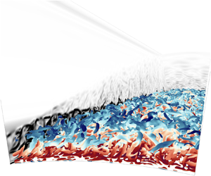
Figure 2. Schematic of the present quasi-spectral viscosity (QSV)-LES of a hypersonic boundary layer over a cone with the volumetric rescaling method. The instantaneous iso-surface of the Q-criterion (second invariant of the velocity gradient tensor) is coloured by temperature. Contours in cross-flow planes show temperature fields in the recycling and rescaling boxes. A contour in a side plane shows the magnitude of the density gradient.

The number of grid points is $N_x \times N_y \times N_{\theta }=1600 \times 256 \times 160$ for the rescaling cases (M7.4-R4.1 and M7.4-R6.4). A coarse mesh of $N_x \times N_y \times N_{\theta }=960 \times 128 \times 84$ is also used in M7.4-R4.1 only to discuss the effects of the rescaling box size in § 4.4. The grid for the laminar–turbulent transition case (M7.4-LT4.1) is $N_x \times N_y \times N_{\theta }=3072 \times 192 \times 160$, which is coarser than the one for M7.4-R4.1 because of the requirements for a larger computational domain. The effects of the different grid resolutions are examined in § 3. The grid spacing is uniform in the streamwise and azimuthal directions. The grid spacing in the wall-normal direction is stretched and clustered at the wall. The grid resolutions at $x=0.85$ m are shown in table 2. They are evaluated as $\Delta x_i^+ \equiv \rho _w \Delta x_i u_{\tau }/\mu _w$, where $u_{\tau } \equiv \sqrt {\tau _w /\rho _w}$ is the friction velocity, $\tau _w$ is the wall-shear stress and $\Delta x_i$ is the grid spacing in the $x_i$ direction; $\Delta x^+$ and $\Delta z^+$ are the grid resolutions in the streamwise and azimuthal directions, respectively. In this paper, $z$ is the coordinate in the azimuthal direction along the curved surface at each $x$ location. The wall-normal grid spacing $\Delta y_1^+$ corresponds to that at the bottom of the domain. The parameter $Re_{\varTheta } \equiv u_{e} \varTheta \rho _{e} / \mu _{e}$ is the Reynolds number based on the momentum thickness $\varTheta$. The parameter $Re_{\tau } \equiv u_{\tau } \delta \rho _{w} / \mu _{w}$ is the friction Reynolds number. The parameter $Re^*_{\tau } \equiv u^*_{\tau, e} \delta \rho _{e} / \mu _{e}$ is a semi-local friction Reynolds number, which accounts for variable density effects (Huang et al. Reference Huang, Coleman and Bradshaw1995). The parameters $\rho _e$ and $\mu _e$ are the density and viscosity at the edge of the boundary layer. The parameter $u^*_{\tau, e} \equiv \sqrt {\tau _w/\rho _e}$ is a semi-local friction velocity. The grid resolutions in the star unit are obtained by $\Delta x_i^* \equiv \Delta x_i^+ Re^*_{\tau }/Re_{\tau }$.

Table 2. Grid resolution at $x=0.85$ m in wall and star units. The parameter $\Delta z$ indicates grid spacing in the azimuthal direction along the curved wall surface. Most results in §§ 4 and 5 are obtained by using the fine meshes. The coarse mesh is used in M7.4-R4.1 only to discuss the effects of the rescaling box size in § 4.4.

The rescaling simulations undergo a long temporal transient until the flow field reaches a steady state, as shown in the authors’ past work (Camillo et al. Reference Camillo, Wagner, Toki and Scalo2023). In the present study, the wall-shear stress and heat flux are monitored and, after they reach the steady state, statistical datasets for the rescaling cases are obtained by spatial averaging in the azimuthal direction and time averaging during a period of approximately $100\delta /u_{\infty }$ based on the boundary layer thickness $\delta$ at $x=0.85$ m. Those for the laminar-to-turbulent case are gathered during a period of approximately $20\delta /u_{\infty }$.

2.3. Volumetric rescaling method

Fluctuations of density, temperature and velocity are rescaled following Stolz & Adams (Reference Stolz and Adams2003) method, with the following modifications: (i) mean profiles of primitive variables are given by RANS calculations, and (ii) fluctuations are extracted from a certain volume and not a plane.

As summarized in § 1.3, general rescaling methods decide mean profiles based on scaling laws such as the Van Driest transformation. However, most scaling laws do not account for the conical expansion of flow in the downstream direction. Therefore, a precursor axisymmetric RANS simulation is carried out in this study and used as the mean inflow instead of scaling laws. Such usage of RANS results was proposed to avoid the drift of mean profiles at the inflow by Sagaut et al. (Reference Sagaut, Garnier, Tromeur, Larchevêque and Labourasse2004).

General rescaling methods extract turbulent fluctuations from a plane at a certain streamwise coordinate, which are then rescaled and added to a mean profile at the inlet boundary. Since the imposed variables do not perfectly satisfy the governing equations at the inlet, adjustments accompanied by non-physical pressure oscillations occur around the rescaling plane. This is especially true with low-dissipation numerics such as the high-order compact finite differencing schemes (Lele Reference Lele1992) used in the present calculation. Spectral-like schemes will not accommodate the non-physical steep flow gradients imposed by a classic planar rescaling strategy, especially at hypersonic conditions.

To allow for proper numerical relaxation of the rescaled fluctuations in a spectral solver, the present study extracts the three-dimensional fluctuating field from a recycling box with a finite extent in the streamwise direction. Such fluctuations are then applied to a rescaling box near the inlet. Numerical trials have shown that excessively small rescaling volumes lead to numerical instabilities, as shown in § 4.4. Due to the spectral nature of the numerics, a sufficient number of streamwise points are needed within the rescaling box to guarantee the robustness of the numerical reconstruction and smoothness of the flow field downstream of it.

The present rescaling procedure is as follows. The formulations for rescaled fluctuations are the same as Stolz & Adams (Reference Stolz and Adams2003) method. The velocity fluctuations $u_i^{\prime }$ in the recycling box are computed as

(2.2)\begin{equation} u_i^{\prime} = u_i - \langle u_i \rangle. \end{equation}

The notations $({\cdot })^{\prime }$ and $({\cdot })^{\prime \prime }$ indicate fluctuations in the average and the Favre average in this paper. The bracket operators $\langle {\cdot } \rangle$ and $\{ {\cdot } \}$ indicate averaging and Favre averaging in time and the azimuthal direction, respectively. The velocity fluctuations imposed in the rescaling box are computed from the extracted fluctuations in the recycling box by using the following scaling:

(2.3a,b)\begin{equation} \frac{u_{i,in}^{\prime}}{u_{\tau}}=G_{in,u_i^{\prime}}(y^+) \quad \mathrm{and} \quad \frac{u_{i,out}^{\prime}}{u_{\tau}} =G_{out,u_i^{\prime}}(\eta). \end{equation}

The subscripts $in$ and $out$ indicate inner- and outer-layer scalings, respectively. Here, $\eta$ is the outer-layer coordinate $y/\delta$ and the functions $G_{in,u_i^{\prime }}$ and $G_{out,u_i^{\prime }}$ are assumed not to depend on the streamwise coordinate $x$. These scaling functions are unknown during the simulation, however, the imposed fluctuations can be obtained by interpolating the fluctuations extracted from the recycling box based on the $y^+$ and $\eta$ coordinates. The density and temperature fluctuations are computed similarly, but they are scaled by their values at the edge of the boundary layer. The scaling laws are expressed as

(2.4a,b)\begin{gather} \frac{T_{in}^{\prime}}{T_{e}}=G_{in,T^{\prime}}(y^+), \quad \frac{T_{out}^{\prime}}{T_{e}}=G_{out,T^{\prime}}(\eta), \end{gather}

(2.5a,b)\begin{gather}\frac{\rho_{in}^{\prime}}{\rho_{e}}=G_{in,\rho^{\prime}}(y^+), \quad \frac{\rho_{out}^{\prime}}{\rho_{e}}=G_{out,\rho^{\prime}}(\eta). \end{gather}

The fluctuations for the inner and outer layers are blended by the weighting function proposed by Lund et al. (Reference Lund, Wu and Squires1998) as

(2.6)\begin{equation} W(\eta)=\frac{1}{2}\left[ 1 + \left(\left. \tanh\left(\frac{\alpha(\eta-b)}{(1-2b)\eta +b}\right) \right/ \tanh (\alpha) \right) \right], \end{equation}

with $\alpha =4$ and $b=0.2$. According to these scaling laws, the imposed flow field in the rescaling box is computed as

(2.7)\begin{gather} u_i^{\prime} = (1-W(\eta))u_{i,in}^{\prime} + W(\eta)u_{i,out}^{\prime}, \end{gather}

(2.8)\begin{gather}T^{\prime} = (1-W(\eta))T_{in}^{\prime} + W(\eta)T_{out}^{\prime}, \end{gather}

(2.9)\begin{gather}\rho^{\prime} = (1-W(\eta))\rho_{in}^{\prime} + W(\eta)\rho_{out}^{\prime}. \end{gather}

In Stolz & Adams (Reference Stolz and Adams2003) method, the fluctuations are computed for the inflow plane. In the volumetric rescaling method, turbulent fluctuations for $0.830\ \mathrm {m} \leq x \leq 0.849\ \mathrm {m}$ (recycling box) are extracted and the fluctuations are scaled and imposed upon the RANS precursor flow for $0.600\ \mathrm {m} \leq x \leq 0.619\ \mathrm {m}$ (rescaling box). The recycling and rescaling boxes have the same number of grid points (e.g. $N_x \times N_y \times N_{\theta }=100 \times 256 \times 160$ for the fine mesh). At each station $x$, i.e. for each ($y$,$\theta$) plane, the rescaled fluctuations are interpolated only in the $y$ direction based on the aforementioned scaling laws. In the present rescaled LES, the imposed fluctuations are separately computed by (2.7)–(2.9) at each $x$ grid point and imposed onto the mean profiles obtained by the precursor RANS. The recycling and rescaling boxes have the same domain lengths in the $x$-direction, while those in the $\theta$-direction are different because the computational domain expands in the direction of going downstream. Therefore, the mapping of the imposed fluctuations is linearly shrunken to match the rescaling box. To impose fluctuations only in a boundary layer, they are attenuated over $y=0.005$ m by a tangent hyperbolic function. The distance between the centres of the recycling and rescaling boxes is $0.23$ m. This length is equivalent to $53 \delta _{i}$ in M7.4-R4.1 and $57 \delta _{i}$ in M7.4-R6.4, where $\delta _{i}$ is the boundary-layer thickness based on 99 % of the free-stream velocity at the inlet ($x=0.6$ m), and it is comparable to other rescaling studies of hypersonic boundary layers (Duan, Choudhari & Zhang Reference Duan, Choudhari and Zhang2016; Huang et al. Reference Huang, Duan and Choudhari2022). The inlet boundary-layer thickness is $\delta _i = 0.0043$ m for M7.4-R4.1 and $0.0040$ m for M7.4-R6.4. In addition, the autocorrelation function in the streamwise direction is investigated in Appendix A, demonstrating that a statistical decorrelation is achieved after approximately 50 mm from the centre of the rescaling box.

Of note, LES results obtained by the present rescaling strategy were compared with experiments conducted in the DLR HEG wind tunnel. The results are discussed with special attention given to the comparison between experimental and computational focused laser differential interferometry signals in Camillo et al. (Reference Camillo, Wagner, Toki and Scalo2023).

2.4. Governing equations

The simulations are performed by solving the spatial filtered compressible Navier–Stokes equations in curvilinear coordinates generalized by Jordan (Reference Jordan1999) and Nagarajan, Lele & Ferziger (Reference Nagarajan, Lele and Ferziger2007). Here, we consider a structured grid in the physical space $\boldsymbol {y}$ to be transformed to computational space $\boldsymbol {x}$ in the present configuration:

(2.10)\begin{gather} x^i = x^i(y_1,y_2, y_3), \end{gather}

(2.11)\begin{gather}y_i = y_i(x^1,x^2, x^3), \end{gather}

where $x^i$ and $y_i$ are the $i$th coordinates of each respective system of reference. The governing equations are given as

(2.12)\begin{gather} \frac{\partial \overline{J \rho}}{\partial t} + \frac{\partial }{\partial x^j}( \overline{J \rho} \tilde v^j)= 0, \end{gather}

(2.13)\begin{gather}\frac{\partial \overline{J \rho}\tilde v^i}{\partial t} + \frac{\partial}{\partial x^j}(\overline{J \rho} \tilde v^i \tilde v^j + \overline{J p} g^{ij} - J \tilde \sigma^{ij} + \overline{J \rho} \tau^{ij})={-}\varGamma^i_{qj}(\overline{J \rho} \tilde v^q \tilde v^j + \overline{J p} g^{qj} - J \tilde \sigma^{qj} + \overline{J \rho} \tau^{qj}), \end{gather}

(2.14)\begin{gather}\frac{\partial \overline{J E}}{\partial t} + \frac{\partial}{\partial x^j}(\overline{J(E + p)}\tilde v^j + J \tilde Q^{j})= \frac{\partial}{\partial x^k}( J \tilde \sigma^{ij}g_{ik}\tilde v^k )- \frac{\partial \overline{J \rho} C_p q^{j} }{\partial x^j}, \end{gather}

where $J$ is the Jacobian of the transformation, which is the determinant of the Jacobi matrix ($J_{ij} = \partial y_i/\partial x^j$), $t$ denotes time, $E$ is total energy and $C_p$ is the specific heat at constant pressure. The parameters $\tau ^{ij}$ and $q^j$ are sub-filter-scale (SFS) stress tensor and SFS temperature flux, and they are written as

(2.15)\begin{gather} \tau^{ij} = \widetilde{v^i v^j} - \tilde v^i \tilde v^j, \end{gather}

(2.16)\begin{gather}q^j = \widetilde{T v^j} - \tilde T \tilde v^j . \end{gather}

These SFS terms are modelled by the QSV method (Sousa & Scalo Reference Sousa and Scalo2022b), which is capable of unifying shock capturing and SFS modelling under a LES mathematical framework based on the concept that both hydrodynamic turbulence and shock formation are characterized by the energy cascade from large to small scales due to nonlinear interactions (Frisch Reference Frisch1995; Gupta & Scalo Reference Gupta and Scalo2018), and they should be treated in a similar fashion. The QSV approach was also developed to be applicable to unstructured grids, via a Legendre spectral viscosity (LSV) method (Sousa & Scalo Reference Sousa and Scalo2022a). In the present study, the SFS kinetic energy advection $\lambda _j =\widetilde {v^k v^k v^j} -\tilde v^k \tilde v^k \tilde v^j$, and the SFS turbulent heat dissipation $\epsilon = \partial (\overline {\sigma ^{ij} v^j})/ \partial x^j - \partial (\tilde \sigma ^{ij} \tilde v^j)/\partial x^j$ are neglected for consistency with the QSV approach published in Sousa & Scalo (Reference Sousa and Scalo2022b) and used in Sousa et al. (Reference Sousa, Wartemann, Wagner and Scalo2024). A closure for these terms has been proposed in a later publication by the same authors Sousa & Scalo (Reference Sousa and Scalo2022a) as part of a new SFS model called LSV applicable to block-spectral schemes for unstructured solvers.

The transformation between $u_i$ and $v^i$ is given by

(2.17)\begin{equation} v^j = u_i \frac{\partial x^j}{\partial y_i}. \end{equation}

The overline $\overline {({\cdot })}$ and tilde $\widetilde {({\cdot })}$ are used for spatial filtering and density-weighted spatial filtering:

(2.18)\begin{gather} \bar{\phi}(x) = \int \phi (x - \xi) G(\xi, x) \, {\rm d} \xi, \end{gather}

(2.19)\begin{gather}\tilde{\phi} = \frac{\overline{\rho \phi}}{\bar{\phi}}, \end{gather}

where $G(\xi, x)$ is the filtering kernel, which depends on filtering types. In (2.12)–(2.14), $g_{ij}$ and $g^{ij}$ are the covariant and contravariant metric tensors, respectively, and $\varGamma ^i_{qj}$ is the Christoffel symbol of the second kind. They are defined as

(2.20)\begin{gather} g_{ij} = \frac{\partial y_i \partial y_j}{\partial x^k \partial x^k}, \end{gather}

(2.21)\begin{gather}g^{ij} = \frac{\partial x^k \partial x^k}{\partial y_i \partial y_j}, \end{gather}

(2.22)\begin{gather}\varGamma^i_{qj} = \frac{\partial x^i}{\partial y_l} \frac{\partial^2 y_l}{\partial x^q \partial x^j}. \end{gather}

In the curvilinear frame of reference the total energy, the viscous stress tensor and the heat flux vector are described by slightly modified relations described below:

(2.23)\begin{gather} \frac{\overline{J p}}{\gamma - 1} = \overline{J E} - \frac{1}{2} \overline{J \rho} g_{ij} \tilde v^i \tilde v^j - \frac{1}{2} \overline{J \rho} g_{ij} \tau^{ij}, \end{gather}

(2.24)\begin{gather}\tilde \sigma^{ij} = \mu(\tilde T) \left(g^{jk} \frac{\partial \tilde v^i}{\partial x^k} + g^{ik} \frac{\partial \tilde v^j}{\partial x^k} - \frac{2}{3} g^{ij}\frac{\partial \tilde v^k}{\partial x^k} \right), \end{gather}

(2.25)\begin{gather}\tilde Q^j ={-} \frac{C_p \mu(\tilde T)}{Pr} g^{ij} \frac{\partial \tilde T}{\partial x^i}, \end{gather}

where $\mu$ is the transport coefficient of viscosity. Sub-filter contributions resulting from nonlinearities involving the temperature dependency of viscosity are neglected for consistency with Sousa et al. (Reference Sousa, Wartemann, Wagner and Scalo2024).

2.5. Numerical methods

In the QSV-LES technique, the governing equations combined with the ideal gas law $p=\rho R_{gas} T$ ($R_{gas}$ is the gas constant) are solved via the sixth-order compact finite difference code CFDSU originally developed by Nagarajan, Lele & Ferziger (Reference Nagarajan, Lele and Ferziger2003) and now under continued development at Purdue. The code CFDSU has been successfully applied to several wall-bounded hypersonic flows (Sousa et al. Reference Sousa, Patel, Chapelier, Wartemann, Wagner and Scalo2019; Chen & Scalo Reference Chen and Scalo2021a,Reference Chen and Scalob; Sousa et al. Reference Sousa, Wartemann, Wagner and Scalo2023; Toki et al. Reference Toki, Sousa, Chen and Scalo2024). The solver adopts a staggered finite difference scheme. Thermodynamic properties such as density, pressure and temperature are stored at cell centres, while velocity components and their associated momentum are stored at cell faces. Since the sixth-order compact scheme is not applicable at boundaries, the order is reduced to the fourth one at two points from each boundary. The time integration is carried out by a four-stage third-order strong stability preserving Runge–Kutta scheme (Gottlieb Reference Gottlieb2005). To ensure time stability, the conservative variables are filtered using a sixth-order compact filter described by Lele (Reference Lele1992). Its filter coefficient is $0.495$. The molecular transport coefficients of viscosity $\mu$ and thermal conductivity $k$ are computed by Sutherland's law.

4.1. Comparison between volumetric rescaling and laminar-to-turbulent transition simulation

Figure 7 shows that the M7.4-LT4.1 case slightly underestimates the heat flux because its grid resolution is relatively coarse. The experimental data show a gradual transition to turbulence between $x = 0.3$ and $0.4$ m, due to the presence of intermittent turbulent structures driven by a low-frequency component of the free-stream noise, which is correctly captured by M7.4-LT4.1. On the other hand, the SA model cannot account for the intermittency and therefore the precursor RANS profile suddenly jumps at $x=0.3$ m. Since mean profiles at the inlet of the present rescaled LES are decided by the precursor RANS and fluctuations are extracted downstream where turbulence is fully developed, the effects of the intermittency are completely ignored in the rescaling simulation. Thus, computational domains of the rescaling cases need to be located sufficiently far from the turbulent transition location.

Figure 7. Comparison of wall-heat flux profiles between the volumetric rescaling simulation M7.4-R4.1 and the laminar-to-turbulent transition simulation M7.4-LT4.1. Data of the precursor RANS and the experiment by Wagner et al. (Reference Wagner, Wartemann, Dittert and Kütemeyer2019) are also included. Correlations for the laminar cone boundary layers (Lees Reference Lees1956) and turbulent ones (White Reference White2006) are given by dash-dotted and dashed lines, respectively.

To examine if the selection of the computational domain is appropriate, figure 8 shows extracted fluctuations of streamwise velocity in the wall-parallel plane at $y=0.5$ mm for M7.4-R4.1 and M7.4-LT4.1. In this paper, the streamwise direction is defined along the cone's surface as well as the $x$-direction. The region between $x=0.6$ and $0.92$ m in M7.4-LT4.1 is enlarged for comparison purposes. The comparison reveals that both cases have long streaky structures, with quite similar lengths and widths. This result implies that the effects of the turbulent intermittency do not reach $x=0.6$ m, and the present rescaling method can generate similar flow fields to those of the laminar-to-turbulent transitional case in the fully turbulent region. Interestingly, the number of streaks in the azimuthal direction appears not to vary after $x=0.6$ m with respect to $x$ coordinates in the M7.4-LT4.1 case, and this is a quite important feature for the performance of the rescaling method. Since the extracted fluctuations are rescaled and recycled at the inlet, the energy spectra of imposed fluctuations should be almost the same as the extracted ones in the azimuthal direction. Therefore, the rescaling method should not be adopted to flow fields including strong variations in the streamwise direction. The almost invariable number of streaks in the laminar-to-turbulent transition case implies that variations of the flow field in the streamwise direction are moderate, and supports the applicability of the rescaling method to the current conical geometry.

Figure 8. Comparison of velocity fluctuation fields in the wall-parallel planes at $y=0.5\ \mathrm {(mm)}$ between (a) the laminar-to-turbulent transition simulation M7.4-LT4.1 and (b) the volumetric rescaling simulation M7.4-R4.1.

Figures 9 and 10 show the azimuthal energy spectra of streamwise velocity and temperature fluctuations for the M7.4-R4.1 (rescaled) and M7.4-LT4.1 (fully transitional) cases. The spectra are extracted at $y^*=15$ and $y^*=300$ at three $x$ locations. A negligible change in the streamwise direction is observed, and a good agreement is observed between M7.4-R4.1 and M7.4-LT4.1 at both $y^*$ locations in general. This result is consistent with the observation of the velocity field in figure 8. A careful observation reveals that the streamwise velocity spectra for $y^*=300$ show a larger value in the M7.4-R4.1 at a small wavenumber even at $x=0.85$ m. The present rescaling calculations have a finer resolution than the fully transitional calculations, which leads to stronger fluctuations, hence a higher value of the spectral energy density, especially at the low wavenumbers. Upon closer inspection, the temperature spectra at $y^*=300$ and $x=0.65$ m of M7.4-R4.1 show a higher fluctuation intensity than M7.4-LT4.1 at the same location. The fluctuations in M7.4-LT4.1 depend on the upstream flow field affected by the laminar-to-turbulent transition process, while those in M7.4-R4.1 are obtained by recycling fluctuations from the downstream. Finally, at the most downstream location of $x=0.85$ m (red lines), the spectra between both cases show the best agreement, indicating that the volumetric rescaling method can ultimately produce turbulent fluctuations with comparable structure to the case accounting for the full laminar-to-turbulent transition path.

Figure 9. Comparison of one-dimensional spectra of streamwise velocity fluctuations in the azimuthal direction between the laminar-to-turbulent transition simulation M7.4-LT4.1 and the volumetric rescaling simulation M7.4-R4.1 for several $x$ locations. The data are extracted at (a) $y^*=15$ and (b) $y^*=300$.

Figure 10. Comparison of one-dimensional spectra of temperature fluctuations in the azimuthal direction between the laminar-to-turbulent transition simulation M7.4-LT4.1 and the volumetric rescaling simulation M7.4-R4.1 for several $x$ locations. The data are extracted at (a) $y^*=15$ and (b) $y^*=300$.

4.2. Recovery length analysis

Since the mean profiles of the primitive variables in the present rescaling method are given by the RANS, a recovery process from the RANS profiles to real turbulent boundary profiles should occur immediately after the rescaling box. To examine the recovery length, figures 11 and 12 compare mean profiles and fluctuation correlations of velocity and temperature at several $x$ locations between M7.4-R4.1 and M7.4-LT4.1. Profiles at $x=0.61$ m are located at the centre of the rescaling box and other profiles are extracted at intervals of $0.05$ m. Mean profiles and fluctuations of velocity are non-dimensionalized by the streamwise velocity at the edge of the boundary layer, and those of temperature by the wall temperature. The wall-normal coordinates are provided in mm to show the development of the boundary layer. The root mean squares (r.m.s.) of fluctuation correlations are computed by Favre average as

(4.1)\begin{gather} u_{i, rms}=\sqrt{\{u_{i}^{\prime\prime} u_{i}^{\prime \prime}\}}, \end{gather}

(4.2)\begin{gather}T_{rms}=\sqrt{\{T^{\prime \prime} T^{\prime \prime}\}}. \end{gather}

Figure 11. Mean profiles of (a) velocity and (b) temperature for $Re_m = 4.1\times 10^6\ \mathrm {m}^{-1}$ cases. Results of the volumetric rescaling simulation M7.4-R4.1 (red solid line) are compared with those of the laminar-to-turbulent transition simulation M7.4-LT4.1 (blue dashed line).

Figure 11 shows that the mean velocity in M7.4-R4.1 agrees well with M7.4-LT4.1 even at $x=0.61$ m, indicating that the SA model has a good prediction of the velocity profile, which is imposed on the rescaling box. As a result, the recovery length for the mean velocity is very short in the present rescaling simulation. On the other hand, the mean temperature is different at the same location, indicating that the SA model has poor accuracy in the prediction of heat transfer in the hypersonic regime, and thus the temperature profile in the rescaling box deviates from that in the M7.4-LT4.1 case. However, the profile in the M7.4-R4.1 case becomes closer to the M7.4-LT4.1 case going downstream and collapses after $x=0.75$ m. The agreement in the downstream indicates that the recovery length for the mean temperature is around $0.15$ m.

By contrast, the fluctuation correlations in figure 12 show several differences between M7.4-R4.1 and M7.4-LT4.1. Both the cases have similar profiles at $x=0.85$ m, indicating that the boundary layer achieves an equilibrium state at this location independently of upstream flow history, also implying a self-similar state of the turbulent fluctuating field at that location. The red circles are obtained by backpropagating the turbulent fluctuating field statistical profiles, scaled by the local boundary-layer thickness, from $x=0.85$ m to the inlet, serving as a reference for what the local state of equilibrium turbulence would look like. A procedural choice has been made in M7.4-R4.1, where fluctuations in the rescaling box (centred at $x=0.61$ m) over $y=5$ mm are suppressed, as mentioned in § 2.2.

Figure 12. Fluctuation correlation profiles of (a) streamwise velocity, (b) wall-normal velocity, (c) spanwise velocity, (d) temperature for $Re_m = 4.1\times 10^6\ \mathrm {m}^{-1}$ cases. Results of the volumetric rescaling simulation M7.4-R4.1 (red solid line) are compared with those of the laminar-to-turbulent transition simulation M7.4-LT4.1 (blue dashed line). Red circles are the result of backpropagating the variance profiles from $x=0.85$ to $x=0.61$ m, rescaling them vertically based on the boundary-layer height, serving as a reference for the local self-similar state of turbulence.

The velocity variance profiles in M7.4-R4.1 agree well with the self-similar reference across the whole domain, while the temperature variance field departs from equilibrium immediately after the rescaling box at $x=0.61$ and is the slowest among the variance profiles to relax to equilibrium, which is only achieved again after $x=0.75$ m, where M7.4-R4.1 and M7.4-LT4.1 are equally far from the final self-similar state. We hypothesize that the present rescaling strategy suffers from the inaccuracy of the mean temperature profiles of the precursor RANS calculation.

The comparison of the mean profiles and fluctuation correlations revealed a recovery length for each variable, and all profiles in the M7.4-R4.1 case reach the equilibrium states after around $x=0.8$ m. This result indicates that the volumetric rescaling method can generate reasonable turbulent flow fields over the cone geometry after a recovery length of 0.2 m, which is equivalent to $43\delta$ based on boundary-layer thickness at the inflow.

The mean profiles in the present rescaling cases are given by the precursor RANS with the SA model and the comparison between the rescaling and laminar-to-turbulent cases revealed that a relatively long recovery length is required for the temperature. The recovery processes for both mean profiles and fluctuations depend on imposed mean profiles in the rescaling box. The SA model has poor accuracy in the prediction of heat transfer in hypersonic boundary layers (Aiken et al. Reference Aiken, Boyd, Duan and Huang2022; Hendrickson et al. Reference Hendrickson, Subbareddy and Candler2022) and thus, recent RANS models including modifications for compressible effects (McDaniel et al. Reference McDaniel, Nichols, Eymann, Starr and Morton2016; Nichols Reference Nichols2019; Danis & Durbin Reference Danis and Durbin2022; Hendrickson et al. Reference Hendrickson, Subbareddy and Candler2022; Parish et al. Reference Parish, Ching, Miller, Beresh and Barone2023; Chen et al. Reference Chen, Gan and Fu2024; Xue et al. Reference Xue, Feng and Zheng2024) have potential to shorten the recovery length, especially as it pertains to the temperature variance field, when they are adopted for the precursor calculation. Wall-modelled LES (WMLES) for compressible boundary layers (Griffin, Fu & Moin Reference Griffin, Fu and Moin2023; Hendrickson et al. Reference Hendrickson, Subbareddy, Candler and Macdonald2023) may also be a candidate for a precursor calculation, with the caveat that mean near-wall profiles in WMLES need to be reconstructed consistently with the model equation used for the inner layer.

4.3. Temperature–velocity relation during the recovery process

The analyses of the recovery length revealed that recovery of temperature is delayed, indicating that the present volume rescaling method requires a longer distance for the thermodynamic equilibrium than the hydrodynamic one. This result implies that the temperature–velocity relation varies during the recovery process. To examine the relation, figure 13 provides the temperature–velocity relation for all cases, including the higher Reynolds number case M7.4-R6.4. The data for M7.4-LT4.1 are shown only after $x=0.61$ m to discuss the fully turbulent region. The mean streamwise velocity and temperature in this figure are normalized by the edge values.

Figure 13. Temperature–velocity relation for (a) M7.4-LT4.1, (b) M7.4-R4.1 and (c) M7.4-R6.4 at several $x$ locations. Black circles in (b) represent the M7.4-LT4.1 data at $x=0.85$ m.

Interestingly, the data for M7.4-LT4.1 in figure 13(a) show excellent collapse, indicating that the temperature–velocity relation achieves self-similarity in the fully turbulent region. On the other hand, the data at $x=0.61$ m of M7.4-R4.1 in figure 13(b) deviate from those of M7.4-LT4.1 because the mean temperature profile is largely different. However, the relation approaches the data of M7.4-LT4.1, going downstream and collapsing after $x=0.75$ m, where the mean temperature showed a good agreement in figure 11. This result implies that the temperature–velocity relation becomes self-similar after the recovery process is completed. The relation for M7.4-R6.4 in figure 13(c) shows almost the same behaviour, indicating that the recovery process is also completed and thermodynamic equilibrium is achieved around $x=0.75$ m in this case.

4.4. Effects of rescaling box size

As mentioned in § 2.3, the present rescaling method imposes fluctuations on the rescaling box for numerical stability of the spectral-like scheme. To investigate the effects of the rescaling box size on simulated flow fields, three different box sizes are tested under the condition of the M7.4-R4.1 case. The tested box sizes are summarized in table 3 and referred to as short, medium and long for simplicity. Coordinates at the beginning and the ending of the rescaling box where fluctuations are imposed, are indicated as $x^s_{imp}$ and $x^e_{imp}$. Similarly, $x^s_{ext}$ and $x^e_{ext}$ are those of the recycling box, from which fluctuations are extracted. The parameter $L_{x,box}$ is the streamwise extent of the boxes in the $x$-direction. In all cases, $x^s_{imp}=0.6$ m and $x^s_{ext}=0.83$ m. The box sizes are changed in the $x$-direction: $L_{x,box}=0.0095$ m for the short box, $L_{x,box}=0.019$ m for the medium box and $L_{x,box}=0.038$ m for the long box. The length of the medium box is generally applied in this paper. The lengths of the short and long boxes are half and double that of the medium one, respectively. The flow fields used in the analyses presented in this section are obtained using the coarse mesh $N_x \times N_y \times N_{\theta }=960 \times 128 \times 84$ shown in table 2.

Table 3. List of the tested rescaling box sizes.

Figure 14 compares pressure fluctuation fields around the rescaling box in the streamwise wall-normal plane and the wall-parallel one to investigate the effects of the rescaling box size on numerical stability. The rescaling box is surrounded by the black dashed line box. The pressure fluctuation with the short box intensifies immediately after the rescaling box. Since a shock wave should not exist in the present flow field, the strong pressure change is unphysical and it can induce numerical instability. The simulation with the short box cannot be sustained due to a numerical blow-up. The pressure fluctuation with the medium box is also strengthened after the rescaling box, however, its strength is so weak that the simulation is sustained. Moreover, the pressure field with the long box is smoothly connected even at the outlet of the rescaling box, indicating that the longer rescaling box can stabilize the simulation, as expected in § 2.3.

Figure 14. Pressure fluctuation fields around the rescaling box in (a,c,e) the streamwise wall-normal plane at the centre in the azimuthal direction, and (b,d,f) the wall-parallel plane at $y=3.5\ \mathrm {mm}$. Panels show (a,b) short box, (c,d) medium box and (e,f) long box. The rescaling box is surrounded by the black dashed line box.

The non-physical pressure fluctuation after the rescaling box may severely affect flow fields downstream, and therefore the box size needs to be sufficiently long. On the other hand, the long rescaling box delays the recovery process from the RANS profiles, since the mean profiles in the rescaling box are fixed to the RANS ones. Thus, the shorter rescaling box is desirable from the perspective of the recovery length and the medium box is used in the present study. To investigate if the present box size is sufficient, wall-heat flux profiles and turbulent fluctuations are compared between the medium and long boxes in figure 15. Although small differences are observed around $x=0.65$ m, the heat fluxes agree well with each other, and fluctuations of streamwise velocity and temperature show excellent collapses after $x=0.7$ m. This result indicates that the effects of the rescaling box size do not extend to $x=0.7$ m, and thus the medium box is sufficiently long to simulate the present conditions. In addition, the collapses imply that fluctuations after $x=0.7$ are independent of the rescaling box, and therefore the recovery length is expected not to be influenced by the box size within the tested conditions.

Figure 15. Comparison of (a) wall-heat flux, (b) fluctuation correlations of streamwise velocity and (c) fluctuation correlations of temperature between different rescaling box sizes.

The short box was also tested with the fine mesh $N_x \times N_y \times N_{\theta }=1600 \times 256 \times 160$, and it numerically blew up as well (not shown). This result suggests that the minimum requirement for the rescaling box size is expected to depend on the size of flow structures rather than grid resolutions. The size of flow structures depends on several flow parameters, and therefore the optimal size of the rescaling box needs to be obtained by a posteriori study.

5.1. Temperature–velocity relationship

Discussion in § 4.3 revealed that the temperature–velocity relation becomes self-similar in the equilibrium state. The estimation of the relation leads to the prediction technique of heat load at the wall, and thus several correlations have been proposed. Huang et al. (Reference Huang, Duan and Choudhari2022) listed correlations, which can be written as

(5.1)\begin{equation} \{T\} = T_w - \left(T_w - T_e - \frac{r_g}{2C_p}{u_e}^2 \right)\frac{\{u\}}{u_e} - \frac{r_g}{2C_p} \{u\}^2, \end{equation}

where the parameter $r_g$ depends on each correlation, and they are summarized in table 4. According to Fernholz & Finley (Reference Fernholz and Finley1980), the Crocco–Busemann relation (Busemann Reference Busemann1931; Crocco Reference Crocco1932) is a classical correlation and Walz (Reference Walz1959) proposed an extended form by considering a recovery factor. Huang et al. (Reference Huang, Bradshaw and Coakley1993) derived their correlation by integrating the energy equation by assuming that the effective Prandtl number is equal to the turbulent Prandtl number in the viscous sublayer. Duan & Martin (Reference Duan and Martin2011) introduced the recovery enthalpy, and demonstrated that the enthalpy–velocity relation collapses, independently of free-stream Mach number. They derived the correlation parameter by the fitting of their DNS data and proposed the correlation by assuming a calorically perfect gas. Zhang et al. (Reference Zhang, Bi, Hussain and She2014) introduced a general recovery factor to modify Walz (Reference Walz1959) equation, and derived its value by considering the turbulent momentum and thermal transport in the wall-normal direction.

Table 4. List of correlations for the temperature–velocity relation; $r\equiv (T_r-T_e)(T_0-T_e)$ is the recovery factor. The turbulent Prandtl number is assumed to be 0.9 in Huang, Bradshaw & Coakley (Reference Huang, Bradshaw and Coakley1993) correlation. The parameter $a=0.8259$ is given by the fitting of DNS data by Duan & Martin (Reference Duan and Martin2011).

These correlations are applied to the present rescaled LES flow fields at $x=0.85$, where the self-similarity is achieved, and compared in figure 16. Correlations of Crocco–Busemann, Walz (Reference Walz1959) and Huang et al. (Reference Huang, Bradshaw and Coakley1993) overestimate the temperature–velocity relation, while those of Duan & Martin (Reference Duan and Martin2011) and Zhang et al. (Reference Zhang, Bi, Hussain and She2014) show good agreements with the present rescaled LES. This result indicates that these correlations can estimate the temperature–velocity relation reasonably well, although they were originally designed for flat plate boundary layers. Furthermore, the present wall-to-recovery temperature ratio is approximately 0.1, and figure 16 demonstrates that the temperature–velocity correlations of Duan & Martin (Reference Duan and Martin2011) and Zhang et al. (Reference Zhang, Bi, Hussain and She2014) remain applicable in such highly cooled hypersonic boundary layers.

Figure 16. Comparison of temperature–velocity relation at $x=0.85$ m between several correlations for (a) M7.4-R4.1 and (b) M7.4-R6.4.

5.2. Turbulent statistics

In this section, several turbulent statistics of the present rescaled LES in the wall-normal direction are shown. All data are extracted at $x=0.85$ m since the recovery length analyses revealed that the recovering process is completed at this location.

Figure 17 provides profiles of velocity fluctuation correlations as a function of $y/\delta$ and $y^*$. The fluctuation correlations are semi-local scaled by mean density and shear stress at the wall. The DNS results of the Mach 11 hypersonic boundary layer on a flat plate for $Re_{\tau }=1138$ by Huang et al. (Reference Huang, Nicholson, Duan, Choudhari and Bowersox2020) are also included in the figure. The velocity fluctuations in the present rescaled LES cases agree well with each other, indicating that velocity fluctuations over the cone geometry can be reasonably scaled in an existing way. The correlation of the streamwise velocity has the peak at almost the same location as the flat plate boundary layer, while the maximum value of the present rescaled LES is larger. Since an LES calculation does not fully resolve the turbulent dissipation field, streamwise velocity fluctuations are generally overestimated (Piomelli, Rouhi & Geurts Reference Piomelli, Rouhi and Geurts2015; Chapelier & Lodato Reference Chapelier and Lodato2016), especially with low-dissipation numerics, and the wall-shear stress underestimated. The correlations drop to almost 0 around $y^*=2000$, whereas the flat plate data do not visibly decrease until $y^*=300$. The discrepancy is attributed to variation in dynamic viscosity in the wall-normal direction. Both the present rescaled LES and the reference DNS have similar $Re_{\tau }\sim 10^3$ and the same wall temperature $T_w=300$ K. By contrast, the free-stream temperature is largely different ($T_{\infty, DNS}=66.5$ K and $T_{\infty, LES}=248$ K or 268 K). The dynamic viscosity decreases toward the edge of the boundary layer in the reference DNS, as a result, $Re^*_{\tau }$, which is computed based on wall shear stress and free-stream properties, is larger in the flat plate DNS ($Re^*_{\tau }\sim 10^4$) than the present rescaled LES ($Re^*_{\tau }\sim 10^3$), in spite of their similar $Re_{\tau }\sim 10^3$. Since $y^*$ at the edge of the boundary layer is equal to $Re^*_{\tau }$, the data of the present rescaled LES drop around $y^*=2000$ whereas those of the reference DNS extend to the farther field.

Figure 17. Velocity fluctuation correlations at $x=0.85$ m as a function of (a) the outer scaling $y/\delta$ and (b) the semi-local wall unit $y^*$. The DNS results of flat plate hypersonic boundary layers by Huang et al. (Reference Huang, Nicholson, Duan, Choudhari and Bowersox2020) are also included.

Figure 18 compares present pressure fluctuation correlations with the incompressible boundary layer on a flat plate for $Re_{\tau }=1145$ by Schlatter & Örlü (Reference Schlatter and Örlü2010). The data in the present rescaled LES are larger than those in the incompressible one around the edge of the boundary layer. The pressure fluctuation in the incompressible flow is attributed to only hydrodynamics, whereas the shocklets also induce the fluctuation in the hypersonic flow. Since the shocklets can propagate over the boundary layer, substantial pressure fluctuation is observed around the edge. Besides, the data in the incompressible flow slightly decrease toward the wall, while those in the present rescaled LES increase below $y^*=10$. This result indicates that strong pressure fluctuations, which are not observed in the incompressible flows, occur in the hypersonic boundary layers.

Figure 18. Pressure fluctuation correlations at $x=0.85$ m as a function of (a) the outer scaling $y/\delta$ and (b) the semi-local wall unit $y^*$. The DNS results of flat plate incompressible boundary layers by Schlatter & Örlü (Reference Schlatter and Örlü2010) are also included.

To explore the effects of the pressure fluctuations on thermodynamic properties, figure 19 shows fluctuation correlations of temperature and density, and figure 20 provides correlation coefficients among density, temperature and pressure. Both fluctuations in figure 19 have their maximum values at the plateau for $0.1< y/\delta <0.6$ and gradually decrease toward the far field. Additionally, both profiles have the second peak around $y^*=5$. The temperature data drop toward the wall because of the iso-thermal boundary condition, while the density profile almost plateaus below $y^*=5$. The density–temperature correlation coefficient $R_{\rho ^\prime T^\prime }$ in figure 20 is around $-$0.8 over $y^*=20$, indicating that the density and temperature are strongly anti-correlated over the buffer region. On the other hand, $R_{\rho ^\prime T^\prime }$ gets close to 0 and the other correlations $R_{p^\prime T^\prime }$ and $R_{p^\prime \rho ^\prime }$ become stronger below $y^*=10$, indicating that temperature and density fluctuations are correlated to pressure in the vicinity of the wall. The profile in figure 18 showed strong fluctuations below $y^*=10$, therefore the enhancement of the correlations $R_{p^\prime T^\prime }$ and $R_{p ^\prime \rho ^\prime }$ implies that the second peaks of temperature and density fluctuations around $y^*=5$ are correlated to the strong pressure fluctuations near the wall. Effects of the strong pressure fluctuations are further discussed in § 5.3 by visualizing the pressure field at the wall.

Figure 19. Fluctuation correlations of (a,b) temperature and (c,d) density at $x=0.85$ m as a function of (a,c) the outer scaling $y/\delta$ and (b,d) the semi-local wall unit $y^*$.

Figure 20. Correlation coefficients of (a) density–temperature, (b) pressure–temperature and (c) pressure–density at $x=0.85$ m.

Understanding the relationship between velocity and temperature is crucial for turbulence modelling, and in particular, many models are developed based on the SRA identified by Morkovin (Reference Morkovin1962). Assuming that the total temperature fluctuations are negligible, the SRA relation is derived for zero-pressure-gradient adiabatic turbulent boundary layers as

(5.2)\begin{gather} Pr_{t}=\frac{\langle \rho \rangle \{ u^{\prime \prime} v^{\prime \prime} \} ( \partial \{T\}/\partial y )}{\langle \rho \rangle \{ v^{\prime \prime} T^{\prime \prime} \}( \partial \{u\}/\partial y )}\approx 1, \end{gather}

(5.3)\begin{gather}-R_{u^{\prime \prime}T^{\prime \prime}}={-}\frac{\{u^{\prime \prime}T^{\prime \prime}\}}{\sqrt{\{{u^{\prime \prime}}^2\}}\sqrt{\{{T^{\prime \prime}}^2}\}}\approx 1, \end{gather}

(5.4)\begin{gather}\frac{\sqrt{\{T^{\prime \prime} T^{\prime \prime}\}}/\{T\}}{( \gamma-1 )M^2(\sqrt{\{u^{\prime \prime} u^{\prime \prime}\}}/\{u\})} \approx 1, \end{gather}

where $M^2=\{u\}^2/(\gamma R_{gas} \{ T \} )$.

Figure 21 shows profiles of the turbulent Prandtl number $Pr_{t}$ as a function of $y/\delta$ and $y^*$. The DNS data of the incompressible flat plate boundary layer (Li et al. Reference Li, Schlatter, Brandt and Henningson2009) and the hypersonic one (Huang et al. Reference Huang, Nicholson, Duan, Choudhari and Bowersox2020) are also included. The value of $Pr_{t}$ in the present rescaled LES slightly decreases for $y/\delta > 0.2$, and its qualitative trend is the same as the reference data. Since the temperature gradient becomes null in the buffer region, vertical fluid motions are not correlated to temperature fluctuations, and $\{ v^{\prime \prime } T^{\prime \prime } \}$ becomes null. As a result, $Pr_{t}$ diverges around $y^*=20$. In addition, $Pr_{t}$ in the cone drops to 0.6 in the viscous sub-layer below $y^*=3$. The comparison with the reference data revealed that such divergence and decrease are not observed in the incompressible boundary layer, but the hypersonic flat plate shows similar behaviours. Therefore, they are attributed to the hypersonic condition, and the turbulent Prandtl number over the hypersonic cone is qualitatively the same as the flat plate. Of note, such decrease of turbulent Prandtl number near the wall is not observable in subsonic wall-bounded flows including strong nonlinear density variations such as supercritical fluids (Kawai Reference Kawai2019; Toki, Teramoto & Okamoto Reference Toki, Teramoto and Okamoto2020; Toki & Bellan Reference Toki and Bellan2021). Thus, the unique turbulent Prandtl number profile is expected to originate not from variation in density but from high Mach numbers.

Figure 21. Turbulent Prandtl number at $x=0.85$ m as a function of (a) the outer scaling $y/\delta$ and (b) the semi-local wall unit $y^*$. The DNS results of flat plate hypersonic boundary layers by Huang et al. (Reference Huang, Nicholson, Duan, Choudhari and Bowersox2020) and those of incompressible ones by Li et al. (Reference Li, Schlatter, Brandt and Henningson2009) are also included.

Figure 22 provides the temperature–velocity correlation coefficient $-R_{u^{\prime \prime }T^{\prime \prime }}$ as a function of $y/\delta$ and $y^*$. The value of $-R_{u^{\prime \prime }T^{\prime \prime }}$ is almost $-1$ below $y^*=5$, indicating that the velocity and temperature fluctuations are strongly correlated in the viscous sub-layer. Since the sign of the temperature gradient is switched in the buffer layer, the fluctuations become anticorrelated over $y^*=50$. The maximum value of the coefficient is around 0.75 at $y/\delta =0.1$ and it gradually decreases toward the far field. The imperfect correlation is also reported in a hypersonic flat plate boundary layer (Huang et al. Reference Huang, Duan and Choudhari2022).

Figure 22. Temperature–velocity correlation coefficient at $x=0.85$ m as a function of (a) the outer scaling $y/\delta$ and (b) the semi-local wall unit $y^*$.

Figure 23(a) depicts the SRA relation of (5.4), and its value deviates from 1 in the entire boundary layer. The SRA relation is derived by neglecting the total temperature fluctuation, however, this assumption does not hold in the present condition because the total temperature varies in the wall-normal direction due to the extremely cold wall temperature. To account for the total temperature variation, Huang et al. (Reference Huang, Coleman and Bradshaw1995) modified the SRA by extending the velocity and temperature fluctuation relationship derived by Gaviglio (Reference Gaviglio1987) and Rubesin (Reference Rubesin1990). Huang et al. (Reference Huang, Coleman and Bradshaw1995) SRA is generally referred to as HSRA and written as

(5.5)\begin{equation} \frac{\sqrt{\langle T^{\prime} T^{\prime}\rangle}/\langle T\rangle}{( \gamma-1 )M^2(\sqrt{\langle u^{\prime} u^{\prime}\rangle}/\langle u\rangle)} \left( 1-\frac{\partial \langle T_0 \rangle}{\partial \langle T \rangle} \right) Pr_{t} \approx 1, \end{equation}

where $T_0$ is the total temperature. The HSRA was developed for periodic channel flows, and therefore ${\partial \langle T_0 \rangle }/{\partial \langle T \rangle }$ considers only variations in the wall-normal direction. Following the original manner, the HSRA in this paper is computed as

(5.6)\begin{equation} \frac{\sqrt{\langle T^{\prime} T^{\prime}\rangle}/\langle T\rangle}{( \gamma-1 )M^2(\sqrt{\langle u^{\prime} u^{\prime}\rangle}/\langle u\rangle)} \left( 1-\frac{\partial \langle T_0 \rangle}{\partial y} \frac{\partial y}{\partial \langle T \rangle} \right) Pr_{t} \approx 1.\end{equation}

The HSRA is shown in figure 23(b). The fluctuation correlations and the derivative of the mean total temperature are computed based on the Reynolds-averaged value in Huang et al. (Reference Huang, Coleman and Bradshaw1995), however, it is sometimes computed based on the Favre-averaged ones (Duan et al. Reference Duan, Beekman and Martin2010; Passiatore et al. Reference Passiatore, Sciacovelli, Cinnella and Pascazio2022). Thus, the HSRA is also computed with the Favre-averaged values as

(5.7)\begin{equation} \frac{\sqrt{\{T^{\prime \prime} T^{\prime \prime}\}}/\{T\}}{( \gamma-1 )M^2(\sqrt{\{u^{\prime \prime} u^{\prime \prime}\}}/\{u\})} \left( 1-\frac{\partial \{ T_0 \}}{\partial y} \frac{\partial y}{\partial \{ T \}} \right) Pr_{t} \approx 1. \end{equation}

The HSRA of (5.7) is referred to as the Favre HSRA, and is shown in figure 23(c). Moreover, Zhang et al. (Reference Zhang, Bi, Hussain and She2014) added the modification of a turbulent Prandtl number to the HSRA as

(5.8)\begin{equation} \frac{\sqrt{\langle T^{\prime} T^{\prime}\rangle}/\langle T\rangle}{( \gamma-1 )M^2(\sqrt{\langle u^{\prime} u^{\prime}\rangle}/\langle u\rangle)} \left( 1-\frac{\partial \langle T_0 \rangle}{\partial y} \frac{\partial y}{\partial \langle T \rangle} \right) Pr_{t, zhang} \approx 1. \end{equation}

The modified turbulent Prandtl number is computed as

(5.9)\begin{equation} Pr_{t,zhang}=\frac{\langle (\rho v)^{\prime} u^{\prime} \rangle ( \partial \langle T\rangle/\partial y )}{\langle (\rho v)^{\prime} T^{\prime} \rangle ( \partial \langle u\rangle/\partial y )}.\end{equation}

The modified HSRA of (5.8) is referred to as Zhang's HSRA and is depicted in figure 23(d). Since Zhang's HSRA is defined by Reynolds-averaged values, its Favre-averaged version is also computed as

(5.10)\begin{equation} \frac{\sqrt{\{T^{\prime \prime} T^{\prime \prime}\}}/\{T\}}{( \gamma-1 )M^2(\sqrt{\{u^{\prime \prime} u^{\prime \prime}\}}/\{u\})} \left( 1-\frac{\partial \{ T_0 \}}{\partial y} \frac{\partial y}{\partial \{ T \}} \right) Pr_{t, zhang} \approx 1. \end{equation}

This relation of (5.10) is referred to as Favre Zhang's HSRA and is provided in figure 23(e). The modified turbulent Prandtl number $Pr_{t,zhang}$ is computed in the same manner as (5.9).

Figure 23. (a) The SRA relation of (5.4), (b) the HSRA of (5.6), (c) the Favre HSRA of (5.7), (d) Zhang's HSRA of (5.8) and (e) the Favre Zhang's HSRA of (5.10) at $x=0.85$ m.

The HSRA shown in figure 23(b) shows improvements compared with the SRA, however, the profile monotonically decreases to 0.7 on going toward the boundary-layer edge ($y/\delta = 1.0$). Meanwhile, the Favre HSRA in figure 23(c) shows a similar trend to the HSRA, however, it drops to only 0.86 at $y/\delta = 1.0$, which is comparable to flat plate compressible boundary layers (Duan et al. Reference Duan, Beekman and Martin2010; Shadloo, Hadjadj & Hussain Reference Shadloo, Hadjadj and Hussain2015; Huang et al. Reference Huang, Duan and Choudhari2022). The improvement indicates that the computation based on the Favre average provides better results in the present highly cooled conical boundary layers. The same trend is observable for Zhang's HSRA. The data obtained by Reynolds average in figure 23(d) decrease to 0.74, while Favre Zhang's HSRA in figure 23(e) shows the best profile among the equations and it is 0.91 at $y/\delta = 1.0$.

A comparison between the M7.4-R4.1 and M7.4-R6.4 in figures 17–23 reveals that the two cases show good agreements in all profiles. They have the same Mach numbers, but the higher Reynolds number is 1.5 times larger than the lower one. Therefore, the agreements indicate that the general turbulent statistics are almost independent of the Reynolds number as far as wall-normal coordinates are considered based on the outer scaling $y/\delta$ or the semi-local unit $y^*$ within the present conditions.

Finally, most obtained statistics are consistent with the referred to flat plate boundary layers in spite of the conical geometry. The consistency with the flat plates implies that the effects of azimuthal expansion are small in the current simulated region. The effects are the most significant around the tip, however, the boundary layer should be laminar until the turbulent transition occurs. Since the transitional point is shifted upstream as an increase in the Reynolds number (Sousa et al. Reference Sousa, Wartemann, Wagner and Scalo2024), the effects of the conical geometry on turbulence are expected to be pronounced in higher Reynolds number flows.

5.3. Flow structure

To understand instantaneous flow structures, fluctuation data of $u$, $T$ and $\rho$ are extracted at various distances from the wall for the M7.4-R4.1 case in figures 24–26. Figure 24 shows fluctuations at $y=0.064\ \mathrm {mm}$ ($y/\delta = 0.01, y^*=5$ at $x=0.85$ m), which are representative of the near-wall region. Figure 25 illustrates data at $y=1.9\ \mathrm {mm}$ ($y/\delta = 0.3, y^*=160$ at $x=0.85$ m), which correspond to the inner layer. Figure 26 depicts information at $y=5.6\ \mathrm {mm}$ ($y/\delta = 0.9, y^*=760$ at $x=0.85$ m), which is located around the edge of the boundary layer. Furthermore, figure 27 provides two-point streamwise correlations of $u$, $T$ and $\rho$ in the streamwise and azimuthal directions at various extracted $y$ locations centred at $x_{ref}=0.8$ m to discuss the statistical size of the boundary-layer structures. The correlation data in the streamwise direction are extracted in both the upstream and downstream directions; the azimuthal direction is periodic, so only positive displacements in the curvilinear coordinate $z$ are shown. Since the present boundary layer is spatially developing, the absolute distance from the wall of a given $y^*$ plane may vary largely in the streamwise direction. Flow structures depend on the $y^*$ value rather than the physical wall-normal distance, and thus the correlations are computed for each $y^*$ plane. Flow structures in the higher Reynolds number case M7.4-R6.4 were also examined, however, its structures are quite similar to the M7.4-R4.1 case, and thus they are not displayed in this paper.

Figure 24. Instantaneous snapshot in the $y=0.064\ \mathrm {mm}$ ($y/\delta = 0.01$, $y^* = 5$ at $x=0.85$ m) wall-parallel plane for M7.4-R4.1. Statistical fluctuation of (a) streamwise velocity, (b) temperature and (c) density.

Figure 25. Instantaneous snapshot in the $y=1.9\ \mathrm {mm}$ ($y/\delta = 0.3$, $y^* = 160$ at $x=0.85$ m) wall-parallel plane for M7.4-R4.1. Statistical fluctuation of (a) streamwise velocity, (b) temperature and (c) density.

Figure 26. Instantaneous snapshot in the $y=5.6\ \mathrm {mm}$ ($y/\delta = 0.9$, $y^* = 760$ at $x=0.85$ m) wall-parallel plane for M7.4-R4.1. Statistical fluctuation of (a) streamwise velocity, (b) temperature and (c) density.

Figure 27. Two-point correlations of streamwise velocity, temperature and density components at $x_{ref}=0.8$ m in the (a,c,e) streamwise and (b,d,f) azimuthal directions. The data are computed for (a,b) $y^*=5$, (c,d) $y^*=161$ and (e,f) $y^*=784$. These $y^*$ locations correspond to (a,b) $y=0.064$ mm, (c,d) $y=1.9$ mm and (e,f) $y=5.6$ mm, respectively.

The velocity field at $y=0.064\ \mathrm {mm}$ in figure 24 shows streaky structures, which have quite thin spacing in the azimuthal direction and a long one in the streamwise direction. Coleman, Kim & Moser (Reference Coleman, Kim and Moser1995) reported that turbulent structures in the supersonic channel flows are elongated in the streamwise direction, and Duan et al. (Reference Duan, Beekman and Martin2010) clarified that the low wall-to-recovery temperature ratio decreases spanwise meandering and increases streamwise coherency in hypersonic boundary layers. The observed long structures in the cone boundary layer are consistent with these past findings. In addition, the present wall-to-recovery temperature ratio is reduced to around 0.1, which is lower than the referred to studies, therefore, the straightness of the streaks is expected to be enhanced. The two-point correlation for $u$ in figure 27(a,b) shows that the correlation does not drop to 0 until $(x-x_{ref})/\delta =9$, while the data drop quickly toward $z/\delta =0.14$ in the azimuthal direction, indicating that the streamwise spacing is approximately 65 times longer than the azimuthal one. The temperature field at this location has quite similar structures to the velocity. The temperature–velocity correlation coefficient $-R_{u^{\prime \prime }T^{\prime \prime }}$ in figure 22 was almost $-1$ below $y^*=5$, and the observed similarity supports the strong correlation. Careful observation reveals that the temperature locally fluctuates in the streamwise direction with short wavelengths, and interestingly, the fluctuations exist only in low-temperature streaks. Since the mean temperature increases from the wall at this $y$ location, low-temperature fluids should originate from the vicinity of the wall. In turbulent boundary layers, upward motions transport the near-wall fluids, and such behaviours are known as ejection events. Temperature streaks attributed to ejection events are observable in supersonic boundary layers (Pirozzoli & Bernardini Reference Pirozzoli and Bernardini2011) and subsonic ones with a temperature gradient (Toki & Bellan Reference Toki and Bellan2021, Reference Toki and Bellan2022), and thus the present low-temperature streaks are expected to be accompanied by ejection events in the same manner as the referred to boundary layers. By contrast, the short-wavelength fluctuations in the temperature streaks were not observed in such boundary layers, implying that these phenomena are attributed to the present hypersonic conditions. The density reflects the temperature field since they are coupled with the equation of state. High-density streaks are correlated to the low-temperature streaks, and vice versa. Similarly to the temperature, strong fluctuations are observed in the high-density streaks.

The velocity field at $y=1.9\ \mathrm {mm}$ in figure 25 shows that the streamwise spacing of both low- and high-speed velocity streaks is shorter and the spanwise spacing is wider than those at $y=0.064\ \mathrm {mm}$. This observation is supported by the two-point correlation shown in figure 27(c,d). Since the mean temperature gradient is switched around $y=0.23\ \mathrm {mm}$ ($y/\delta =0.037$) as shown in figure 11, the high-temperature streaks can be observed at the same locations of low-speed streaks. The anti-correlation is consistent with $-R_{u^{\prime \prime }T^{\prime \prime }}$ in figure 22. In contrast, low-temperature streaks are not clear despite the clear high-velocity streaks. This result indicates that the weak anti-correlation between the velocity and temperature in figure 22 is attributed to downward vertical motions (sweep events) because the mean temperature decreases toward the far field. In addition, the two-point correlations of temperature indicate shorter and wider structures than the streamwise velocity field. The dissimilarity was also observed in supersonic and subsonic boundary layers (Pirozzoli & Bernardini Reference Pirozzoli and Bernardini2011; Toki & Bellan Reference Toki and Bellan2021, Reference Toki and Bellan2022). The temperature fluctuations observed in the near-wall low-temperature streaks do not exist in this plane, indicating that they only appear in the vicinity of the wall. The density field reflects the temperature field, similarly to the near-wall region. Since the density is inversely proportional to the temperature, low-density streaks are clear while high-density streaks are not clearly observable.

At $y=5.6\ \mathrm {mm}$, streaks no longer exist in any contours, and the two-point correlations quickly drop to 0 in the streamwise direction for all components. Fluctuations are quite weak in the upstream before $x=0.65$ m because the edge of the boundary layer does not reach this plane. The similarity between the velocity and temperature becomes further obscure, which is consistent with the low $-R_{u^{\prime \prime }T^{\prime \prime }}$ in figure 22. Some high-temperature and low-density fluctuations are shaped akin to a mushroom-like structure reported in supersonic boundary layers by Pirozzoli & Bernardini (Reference Pirozzoli and Bernardini2011) despite the present hypersonic Mach number.

Some features in the inner and outer layers are similar to supersonic and subsonic boundary layers, whereas the strong fluctuations in low-temperature streaks in the vicinity of the wall have not been reported in such boundary layers. In addition, pressure fluctuations shown in figure 18 are enhanced near the wall, and thus a straightforward expectation is that the hypersonic condition induces the strong pressure fluctuations, and the temperature ones result from them. To further investigate the near-wall phenomenon, figure 28 shows instantaneous contours of pressure fluctuations at the wall. Moreover, the wall-heat flux contour is also included to investigate the effects of the temperature fluctuations on the heat load at the wall.

Figure 28. Instantaneous snapshot at the wall for M7.4-R4.1: (a) pressure fluctuation and (b) wall-heat flux.

The wall-pressure fluctuation field shows strong pressure oscillations in the streamwise direction. A careful comparison with the near-wall temperature fluctuation in figure 24(b) clarifies that the pressure oscillations are correlated to the temperature fluctuations. This observation is consistent with the near-wall behaviour of the pressure–temperature correlation in figure 20. Similar pressure oscillations were originally observed in supersonic and hypersonic channel flows, and they are called alternating positive and negative structures by Tang et al. (Reference Tang, Zhao, Wan and Liu2020) or trapped waves by Chen & Scalo (Reference Chen and Scalo2021b). Similar pressure structures were also recently observed in hypersonic boundary layers by Xu, Wang & Chen (Reference Xu, Wang and Chen2023) and Huang et al. (Reference Huang, Duan, Casper, Wagnild and Bitter2024). Following Chen & Scalo (Reference Chen and Scalo2021b), we call the pressure oscillations a trapped wave in this paper. Chen & Scalo (Reference Chen and Scalo2021b) mentioned the possibility that the trapped wave resembles the amplification of second-mode waves in cooled hypersonic boundary layers, in which an enhancement in wall cooling yields a stronger instability in the hypersonic laminar boundary-layer flow. Research about the instability, which is summarized in Fedorov (Reference Fedorov2011), revealed that acoustic rays are trapped between the wall and the sonic line owing to the presence of a region of supersonic mean flow relative to the disturbance phase velocity. The observation of figures 24(b) and 28(a) clarifies that the trapped waves exist only in fluids ejected from the wall, implying that the waves are induced by the interaction between the boundary layer and the wall as well as the second-mode waves.

Effects of the trapped waves extend to the wall-heat flux shown in figure 28(b). The trapped waves involve strong fluid expansion and compression, and therefore strong and localized temperature fluctuations also occur near the wall, as shown in figure 24(b). Since the wall-heat flux reflects the near-wall temperature field, its structures are similar to those of the temperature. The heat flux field has streaky structures and oscillating patterns attributed to the trapped waves are also observed, indicating that the trapped waves induce strong fluctuations of wall-heat flux. Similar structures of wall-heat flux and wall-shear stress were also reported for hypersonic boundary layers over flat plates by Roy et al. (Reference Roy, Kuchta and Duan2024). In addition, the fluid temperature locally becomes below the wall temperature in the vicinity of the wall due to the strong fluid expansion. As a result, the wall-heat flux shows local negative values, indicating that the boundary layer locally absorbs heat from the wall against the statistical direction.

For further investigation, figure 29 shows a time series of the pressure fluctuations at the wall for $0.76\ \mathrm {m} \leq x \leq 0.84\ \mathrm {m}$ and $-0.014\ \mathrm {m} \leq z \leq 0\ \mathrm {m}$. The $x$ and $z$ coordinates are normalized by the wall viscous length scale $l^+ \equiv \mu _{w} / \sqrt {\rho _{w} \tau _{w}}$ at $x_{ref}=0.8\ \mathrm {m}$. The instantaneous snapshots are extracted at 7 different times $t$ every $4.8\ \mathrm {\mu }\mathrm {s}$. A selected series of trapped waves is surrounded by the white dashed line square box at each $t$ to explore its propagation. The fluctuation profiles along the white dash-dotted line are also shown in figure 30. Fluctuations of wall-heat flux are included as well and the extracted fluctuations are non-dimensionalized by local mean values. A wavelength in the streamwise direction $\lambda _x^+$ is estimated based on a distance between positive peaks and included. The wavelength is also normalized by $l^+$.

Figure 29. Contours of pressure fluctuations at the wall in M7.4-R4.1 at (a) $t=0\ \mathrm {\mu }\mathrm {s}$, (b) $t=4.8\ \mathrm {\mu }\mathrm {s}$, (c) $t=9.6\ \mathrm {\mu }\mathrm {s}$, (d) $t=14.4\ \mathrm {\mu }\mathrm {s}$, (e) $t=19.2\ \mathrm {\mu }\mathrm {s}$, (f) $t=24.0\ \mathrm {\mu }\mathrm {s}$ and (g) $t=28.8\ \mathrm {\mu }\mathrm {s}$. A selected series of trapped waves is surrounded by the white dashed line square box at each $t$ to explore its propagation. Profiles of pressure fluctuations along the white dash-dotted lines are extracted and shown in figure 30.

Figure 30. Profiles of pressure and wall-heat flux fluctuations at the wall along the white dashed-dotted lines in figure 29 at (a) $t=0\ \mathrm {\mu }\mathrm {s}$, (b) $t=4.8\ \mathrm {\mu }\mathrm {s}$, (c) $t=9.6\ \mathrm {\mu }\mathrm {s}$, (d) $t=14.4\ \mathrm {\mu }\mathrm {s}$, (e) $t=19.2\ \mathrm {\mu }\mathrm {s}$, (f) $t=24.0\ \mathrm {\mu }\mathrm {s}$ and (g) $t=28.8\ \mathrm {\mu }\mathrm {s}$.

The trapped waves in the box of the white dashed line propagate in the streamwise direction. The extracted pressure profile in figure 30(a) shows that the strength of the fluctuation is around 50 % of the local mean pressure and $\lambda _x^+$ is around 300 at $t=0\ \mathrm {\mu }\mathrm {s}$. The pressure fluctuation reaches 100 % of the local mean pressure, and $\lambda _x^+$ is reduced to 225 at $t=9.6\ \mathrm {\mu }\mathrm {s}$. After that, $\lambda _x^+$ gradually increases to around 570 as $t$ progresses, and the selected trapped waves almost disappear at $t=28.8\ \mathrm {\mu }\mathrm {s}$. The observation of the time history implies that their wavelength is approximately 200 to 600 times as long as the wall viscous length scale $l^+$, which is around $5\ \mathrm {\mu }\mathrm {m}$. The boundary-layer thickness $\delta$ is $5.9\ \mathrm {mm}$ at $x_{ref}=0.8\ \mathrm {m}$, and therefore the wavelength is around $0.17$ to $0.5\delta$. In addition, the series of trapped waves travel around $9000l^+$ during $28.8\ \mathrm {\mu }\mathrm {s}$ and disappears. This length corresponds to $0.045 \ \mathrm {m} \sim 7.6 \delta$ and their travel speed is around $1560\ \mathrm {ms}^{-1}$ corresponding to Mach 4.5 based on the wall temperature. The frequency of the trapped waves can be estimated as between $520$ and $1560$ kHz from the speed and wavelength. The short travel distance indicates that the trapped waves repeat appearances and disappearances, and do not circulate by the rescaling method. Furthermore, the occurrence of the trapped waves indicates that the second-mode instability in the hypersonic regime is important even in turbulent states.

Profiles of wall-heat flux fluctuations in figure 30 display a high degree of correlation with the wall-pressure fluctuations, supporting the idea that the aforementioned trapped waves may be responsible for the strong overshoots in the wall-heat flux, which may reach two times the mean (e.g. see $t=14.4\ \mathrm {\mu }\mathrm {s}$). Pressure fluctuations are dominated by inviscid mechanisms and follow the wave propagation velocity. By contrast, fluctuations of wall-heat flux depend on the temperature of the near-fluid parcels, regulated by convective wall-normal transport mechanisms, ultimately limited by molecular diffusion in the thermal sublayer. This correlation is surprising since trapped waves seem to exist only in regions of fluid ejection (see figure 24), which is responsible for negative fluctuations in heat flux. However, this does suggest that the trapped waves are responsible for regulating the convective supply of colder or hotter (than the wall) fluid parcels at the edge of the thermal sublayer. More investigation into this phenomenological correlation is warranted and deferred to future studies.

Figure 31 extracts the pressure fluctuation field below $y^+=150$ in the $(x,y)$ plane along the dashed-dotted lines in the middle of the dashed white boxes in figure 29 to investigate structures of the trapped waves in the wall-normal direction. Contour lines of local Mach number are given by dashed lines. The wall unit $y^+$ is adopted because the semi-local unit $y^*$ does not constitute a linear mapping against the wall-normal coordinates. From $t=0$ to $t=9.6\ \mathrm {\mu }\mathrm {s}$, the wavelength becomes shorter and the fluctuation is enhanced only below $y^+=30 (y^*=9)$. Interestingly, these strong fluctuations extend to the contour line of Mach 1.0 and do not cross the line of Mach 2.0, indicating that the fluctuations are trapped by the sonic line as Chen & Scalo (Reference Chen and Scalo2021b) expected; not to be confused with the relative sonic line, which is defined in the context of transitional hypersonic flows (Fedorov Reference Fedorov2011). There is an uplift in the sonic line after $t=14.4\ \mathrm {\mu }\mathrm {s}$, reaching $y^+=50$ $(y^*=15)$ at $t=24.0\ \mathrm {\mu }\mathrm {s}$. The trapped waves remain attached to the wall until, in this particular example, they dissipate at $t=28.8\ \mathrm {\mu }\mathrm {s}$.

Figure 31. Contours of pressure fluctuations in the $(x,y)$ plane below $y^+=150$ in M7.4-R4.1 at (a) $t=0\ \mathrm {\mu }\mathrm {s}$, (b) $t=4.8\ \mathrm {\mu }\mathrm {s}$, (c) $t=9.6\ \mathrm {\mu }\mathrm {s}$, (d) $t=14.4\ \mathrm {\mu }\mathrm {s}$, (e) $t=19.2\ \mathrm {\mu }\mathrm {s}$, (f) $t=24.0\ \mathrm {\mu }\mathrm {s}$ and (g) $t=28.8\ \mathrm {\mu }\mathrm {s}$. Contour lines of local Mach number are given by dashed lines. The visualized regions are selected along the white dash-dotted lines shown in figure 29.

To quantitatively explore their behaviour, figure 32 provides energy spectra of pressure fluctuations in time at $x=0.85$ m for several $y$ locations and figure 33 shows the probability density function (p.d.f.) of pressure fluctuations for the same locations. The sampling frequency is 25 MHz and the data are collected for $0.16$ ms. The spectra are computed with the Hann window and segments of 1000 points and 70 % overlap.

Figure 32. Energy spectra of pressure fluctuations in time at $x=0.85$ m for the M7.4-R4.1 case for several $y^*$ locations. The spectra are shown in (a) the linear scale and (b) the logarithmic scale.

Figure 33. The p.d.f. of pressure fluctuations at $x=0.85$ m for the M7.4-R4.1 case for several $y^*$ locations. The data are shown in (a) the linear scale and (b) the logarithmic scale.

The energy spectra at $y=1.9$ mm and $5.6$ mm show clear energy cascade from $f=100$ to $5000$ kHz. The sudden slope change around $f=5000$ kHz corresponds to the frequency constraint due to the present grid resolution, as discussed in the authors’ past work (Camillo et al. Reference Camillo, Wagner, Toki and Scalo2023). On the other hand, the spectra at the wall and $y=0.064$ mm show a plateau peak between $500$ and $700$ kHz. The frequency is comparable to the estimated one of the trapped waves from figure 30, and thus this peak is attributed to the trapped waves. The absence of the peak for $y=1.9$ mm and $5.6$ mm is consistent with the non-existence of trapped waves over the sonic line in figure 31.

Figure 33 shows that the probability density at the wall and $y=0.064$ mm extends from $-0.5$ to $0.5$, while the data for $y=1.9$ and $5.6$ mm are below 0.1 at $p^{\prime }/\langle p \rangle = \pm 0.3$. As shown in figure 30, the trapped waves can be characterized by strong pressure fluctuations, and such strong fluctuations are not observed away from the wall. Therefore the p.d.f. for $|p_w^{\prime }|/\langle p \rangle > 0.3$ mainly originates from the trapped waves. The probability of such strong pressure fluctuations can be obtained by integrating the p.d.f. at the wall for $|p_w^{\prime }|/\langle p \rangle > 0.3$, and the integrated value is 7.3 %. This result indicates that strong pressure fluctuations associated with the trapped waves cover 7.3 % of the wall surface.