

1. Introduction
In recent decades, the mass balance of most alpine glaciers has been markedly negative, and these glaciers have undergone an acceleration of mass loss and terminal retreat (Reference Dyurgerov and MeierDyurgerov and Meier, 1997, Reference Dyurgerov and Meier2000, Reference Dyurgerov and Meier2005; Reference Cogley and AdamsCogley and Adams, 1998; Reference Haeberli, Frauenfelder, Hoelzle and MaischHaeberli and others, 1999; Reference OerlemansOerlemans, 2000; Reference DyurgerovDyurgerov, 2001; Reference Meier, Dyurgerov and McCabeMeier and others, 2003; Reference Paul, Kääb, Maisch, Kellenberger and HaeberliPaul and others, 2004). In the Canadian Cordillera, these conditions have been associated with unusually warm mean annual air temperatures and a reduction in winter snowfall since 1976 (Reference Moore and DemuthMoore and Demuth, 2001; Reference Demuth, Keller, Demuth, Munro and YoungDemuth and Keller, 2006). The resulting more rapid rise of the transient snowline on glaciers during the summer has resulted in a greater amount of ablation due to the earlier exposure of lower-albedo glacial ice. Continued mass loss and recession of glaciers is expected for the foreseeable future as a result of further increases in global temperature (Reference McCarthy, Canziani, Leary, Dokken and WhiteMcCarthy and others, 2001).
Concern exists over the loss of glaciers in the Cordillera since a reduction in glacier area will likely lead to an eventual reduction in late-summer glacial meltwater runoff contributions in headwater catchments. Although only a small percentage of the total annual runoff of higher-order streams and rivers in the Cordillera is contributed by glacial melt, mountain glaciers tend to moderate interannual variability in stream-flow and help to maintain higher runoff volume during extreme warm and dry periods (Reference Fountain and TangbornFountain and Tangborn, 1985; Reference Hopkinson and YoungHopkinson and Young, 1998). In the headwaters of the North Saskatchewan River, eastern Rocky Mountains, the capacity of glaciers to regulate late-summer stream-flow is already in decline (M.N. Demuth and A. Pietroniro, unpublished information). A decrease in the late-summer flow of glacier-fed rivers throughout British Columbia has also been observed, indicating that most glaciers here have already passed the phase of warming-induced runoff increases (Reference Stahl and MooreStahl and Moore, 2006).
Glacier-monitoring efforts in the Canadian Cordillera have focused on a few selected glaciers (e.g. Peyto, Athabasca and Place Glaciers). There is presently, however, a need for a regional inventory of glacier coverage and changes in glacier extent. The acquisition of such inventories from remotely sensed imagery repeated at intervals of several decades is a primary objective of the international Global Land Ice Measurements from Space (GLIMS) project (Reference BishopBishop and others, 2004). At a regional level, part of the aim of the Western Canadian Cryospheric Network (WC2N) is to establish recent past and current glacier extent in the Cordillera. The objective of the present study is therefore to quantify the total glacier area and volume, and their changes over the past several decades, in a portion of the southern Canadian Cordillera that has received little previous attention. Such information is essential for evaluation of the impacts of ice loss on regional water resources and for validation of models of glacier–climate interaction.
2. Study Area
The study area is an east–west transect within the approximate region 50–51˚ N, 115–125˚W, encompassing the Rocky, Columbia and Coast Mountains (Fig. 1). Glaciers cover an area of roughly 2690 km2 in this region. Most of this ice is found within the Coast Mountains, where several extensive (i.e. >100km2) icefields and their outlet glaciers, along with many large valley glaciers, account for approximately 85% of the total glacier area. The Purcell Mountains contain a further 9% of the total area of glacier ice in the region. Here, there are several small icefields and numerous smaller valley and cirque glaciers. The remaining mountain ranges within the study area contain only small (i.e. <4 km2) cirque and hanging glaciers, which comprise a small fraction of the total ice cover. There are no glaciers within the central region of British Columbia.
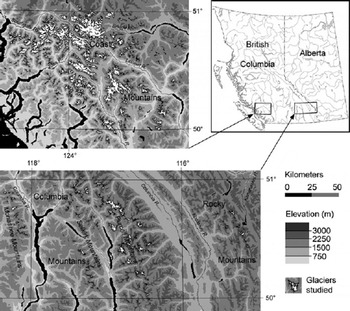
Fig. 1. Distribution of the glaciers and ice fields analyzed in this study.
Climate varies considerably across the southern Cordillera. Annual precipitation declines eastwards from an average of 3500 mm or more in the uplands of the coastal region, to 1500–2500mm in the central Columbia Mountains and 1000–1500mm in the Rockies (Environment Canada, http://www.cccma.bc.ec.gc.ca/hccd/index.shtml).The Coast Mountains have a maritime climate with observed average January and July temperatures of –15˚C and 10˚C respectively, and receive most precipitation in the winter months. Both continental and maritime air masses influence southern interior British Columbia, and precipitation is distributed more uniformly throughout the year. Winter temperature is similar to the coast, but summer temperature ranges from 15˚C to 20˚C. The eastern ranges of the Rockies are dominated by continental air masses, and January temperature averages –15 to –20˚C, while summer temperatures are similar to those in the Columbia Mountains.
3. Methods
Changes in glacier surface area were determined from comparison of remotely sensed imagery acquired in 1951/ 52 over the Columbia and Rocky Mountains, in 1964/65 over the Coast Mountains and in 2001/02 over the entire study area. Ice margins for each time period were delineated using Geographic Information Systems (GIS) software, and compared to obtain measurements of the net area change of individual glaciers. Estimates of ice volume for each period were based on measured surface area, and net volume loss was determined as the difference between estimates.
3.1. Sources of data
The satellite imagery used consists of three Landsat 7 Enhanced Thematic Mapper Plus (ETM+) scenes acquired on 14 September 2001 (path 44, row 25), 23 September 2001 (path 43, row 25) and 13 September 2002 (path 48, row 25). These scenes were obtained from the Geogratis website (http://geogratis.cgdi.gc.ca/) of Natural Resources Canada as Landsat 7 Orthorectified Imagery over Canada, which is derived from Landsat 7 raw image level L1G (i.e. radio-metrically and systematically corrected) processed data. The planimetric error associated with this imagery is reported to be ±30m or less with a 90% level of confidence. The aerial photography consists of British Columbia government photos acquired in late July 1964/65 over the Coast Mountains (~1 : 30 000 scale), and from late July through September 1951/52 over the Columbia and Rocky Mountains (~1 : 50 000 scale). The digital elevation model (DEM) used in this study is part of the DMTI Spatial Inc. dataset, which was created from interpolation of the Canadian National Topographic Database (NTDB) 1 : 50 000 scale digital mapping (Standards and Specifications V3.0 and later). This DEM represents the surface elevation at the time of aerial photograph acquisition. Individual DEMs were projected to the NAD83 Universal Transverse Mercator (UTM) grid at 30m resolution, and vertical error was estimated to be ±20m (i.e. half the contour interval of the NTDB mapping).
3.2. Image preparation and geometric correction
The satellite imagery was obtained with spatial reference to the Lambert Conformal Conic map projection with standard parallels of 49˚ and 77˚N on the NAD83 datum and GRS 1980 ellipsoid, and subsequently projected in UTM coordinates. Data fusion was performed to enhance the apparent resolution of the imagery using the FUSION function in the PCI GeomaticaTM Xpace module, where ETM+ bands 2, 3 and 4 (30m resolution) were combined with the panchromatic band 8 (15m resolution). Original aerial photo prints were scanned at 300 dpi (~4m ground resolution (1 : 50 000 scale photos); ~2.5m resolution (1 : 30 000 scale photos)) and spatially referenced to the fused ETM+ Orthorectified Imagery using the thin-plate spline math model in PCI OrthoengineTM. This model fits the ground-control points (GCPs) exactly, and warping is distributed throughout the image, with minimum curvature between points becoming linear away from the GCPs. Individual photos were referenced to the ETM+ imagery by selecting 15–20 GCPs that were clearly identifiable in both images, with most of the points chosen on stable terrain immediately adjacent to glacier termini and areas where the photos showed glacier change.
3.3. Ice-margin delineation
Ice margins and interior bedrock outcrops were delineated from the 2001/02 imagery using on-screen digitizing techniques in ArcMapTM 8.3 GIS. Discrete ice masses and outcrops were defined by manually digitizing a series of points to construct polygon shapefiles, and the interior bedrock polygons were used to clip the ice extent to create an ‘ice surface only’ polygon. Separate polygons representing ice fields and diverging glaciers were then clipped to allow area change measurements to be associated with individual drainage catchments. This was done by manually cutting the polygons along the ice divides, which were identified using topographic contours derived from the DEM and the ‘Basin’ utility in the Spatial Analyst extension of ArcMapTM. Where the DEM clearly misrepresents the ice surface, boundaries were defined by visual interpretation of the ETM+ imagery.
Ice margins in the lower portion of each glacier were derived in a similar manner from the 1951/52 and 1964/65 geometrically corrected aerial photos. For the accumulation zones of individual glaciers, margins were copied from the 2001/02 polygons, except in situations where obvious change had occurred, when the margin was also adjusted.
3.4. Area and volume calculations
Area measurements for the individual glaciers were derived directly from the shapefiles in ArcMapTM. Tabulated areas for each time period were then compared to determine changes. Where a glacier had split into several distinct ice masses, the net area change was based on the total area of the individual glaciers represented in the 2001/02 shapefile.
Area measurements were used to estimate glacier volume using a volume–area scaling relationship (Reference Chen and OhmuraChen and Ohmura, 1990; Reference Bahr, Meier and PeckhamBahr and others, 1997). The volume, V (in 106m3), of an alpine valley glacier is related to its surface area, S (in 106m2), as:
for which observations of a wide range of glaciers worldwide give values of 28.5 and 1.36 for c 0 and c 1 respectively. These values have been found to be suitable for glaciers within the southern Cordillera, where glacier volume change in the Coast Mountains has been determined from comparison of multitemporal DEMs (personal communication from B. Menounos, 2005) and from field-based reconstruction of several Little Ice Age (LIA) glacier surfaces in the Purcell (Columbia) and Rocky Mountains (Reference DeBeerDeBeer, 2006). Volume changes were determined by differencing the volume estimates for each period. Where a glacier had disintegrated, Equation (1) was applied to the total area of all separate ice masses in order to minimize errors in the estimated volume change.
Although this approach is empirical, Reference Bahr, Meier and PeckhamBahr and others (1997) have demonstrated that there is a physical basis for it. Other methods, such as the shallow-ice approximation (e.g. Reference Driedger and KennardDriedger and Kennard, 1986), were not considered due to the limiting assumptions inherent in these approaches (e.g. that longitudinal stresses are not an important component of the glacier force balance).
3.5. Error estimation
Potential error associated with measurements of the 2001/02 glacier surface area depends upon the accuracy with which the margin of individual glaciers can be identified and digitized. This depends upon the image resolution, the snow conditions and the contrast between the ice and adjacent terrain. The uncertainties associated with the regional measurements of glacier area were estimated from a detailed analysis of small samples of regionally representative glaciers. For each sample, the fraction of the total ice perimeter affected by various types of obscurities was determined, and a maximum offset distance between the digitized boundary and the true ice margin was assigned to each type of obscurity. The error was then scaled up to the entire set of glaciers by multiplying the fraction of the regional ice perimeter length by the estimated offset distance for the various obscurity types.
For unobscured sections of ice margin, which represent 82–87% of the perimeter of the various samples, measurement uncertainty was judged to be no greater than the resolution of the fused ETM+ imagery (±15 m). Where continuous debris cover or shadows obscure ice margins (each representing 3–8% of the sample perimeters), the error was estimated to be ±45 m. For debris-covered sections, the estimate was based on a comparison between measurements derived from the ETM+ imagery and field observations at several sites in the Rocky and Purcell Mountains. In general, accurate manual delineation was possible for debris-covered termini because of the difference in illumination at the glacier boundary. Where the margin is obscured by shadow, a contrast-stretching function was applied to the ETM+ imagery to improve the ability to detect the ice–rock boundary. The uncertainty is greatest where late-lying snow obscures the ice margin (1–4% of the sample perimeters) or could be misinterpreted as glacier ice. Measures taken to avoid misclassification in such cases included comparison with other remotely sensed imagery and detection of crevasses or emerging bare ice (see Fig. 3 further below). Here error was estimated to be ±90m for the ice margin.
Planimetric error within the orthorectified ETM+ imagery was not considered to be significant because the positional error of this imagery is unlikely to be random, and correspondence between locations within the imagery and their true ground position is unimportant in terms of the measurement of surface area. Similarly, this error has no effect on the measurements of area change, as the uncertainty in these measurements depends only on the accuracy of the co-registration between the aerial photography and the ETM+ imagery, and the ability to correctly identify the ice margins.
Repeated measurements of surface area change were made for 16 randomly chosen glaciers, in order to estimate the uncertainty associated with these measurements. Measurements were made for a range of different magnitudes of absolute area change and for aerial photos with differing amounts of snow cover, where extreme potential positions of the ice margin were digitized to determine both the maximum and minimum change in area. Based on these estimates of uncertainty, the relative uncertainty was estimated for the entire set of glacier area change measurements.
In addition to the potential error resulting from the digitizing process, error may also arise due to imperfect co-registration between the aerial photography and the ETM+ imagery. This was accounted for by measuring the length of perimeter digitized from the aerial photography for the same test glaciers as above, and multiplying this length by the co-registration error. Because the model used in the geometric correction process fits the GCPs exactly, co-registration error near the control points was estimated to be equal to the fused ETM+ image resolution (i.e. ±15 m) on average. However, since it is assumed to be independent and randomly distributed, 50% of this error was chosen as a more reasonable estimate. The resulting estimates of uncertainty, which depend on the absolute change in area, were used to estimate the relative uncertainty for all area change measurements.
The total error (δQ) related to the 2001/02 surface area, as well as that related to the measured change in area, was calculated as:
where δq 1,. . .,δqn represent the individual uncertainties in surface area associated with each type of image problem. The actual error is likely overestimated, as this assumes a maximum digitizing offset over all linework derived from the ETM+ imagery and the aerial photography. It is more likely that multiple random errors in the digitizing process roughly cancel.
Estimates of glacier volume and volume change over the study period are also subject to uncertainty. This is a result of error in the measurements of area, from which ice volume was estimated, and the choice of parameters used in the volume–area scaling relationship. For glaciers that have undergone significant ice loss, uncertainty due to the choice of scaling parameters is typically an order of magnitude greater than that due to area measurement error. Since the measurement error is likely overestimated to begin with, uncertainty in the volume estimates attributable to the errors in the area measurements was considered to be negligible. A larger potential source of error results from the fact that the approach used assumes that the parameters c 0 and c 1 in Equation (1) are spatially and temporally constant. This may not necessarily be true, so large errors may potentially arise when calculating a small quantity (volume change) as the difference between two estimates of a large quantity (volume), each of which has a large uncertainty. However, if volume–area scaling is applied consistently to a large sample of glaciers (>1500 in this study), the errors involved in applying the method to individual glaciers tend to cancel and the method provides a useful basis for estimating volume change at the regional scale, even though estimates for individual glaciers may not be reliable. Thus, the approach provides a useful way of indicating where the most significant volume losses have occurred even though the actual magnitudes should, in future, be verified by direct measurement.
To set limits on the uncertainty in the overall volume estimates, c 0 and c 1 in Equation (1) were varied to reflect the range of estimates of these parameters that have been derived empirically for different regions (e.g. Reference Chen and OhmuraChen and Ohmura, 1990) and on the basis of physical considerations (e.g. Reference Bahr, Meier and PeckhamBahr and others, 1997). The maximum difference between the resulting volume estimates was taken as a measure of the uncertainty in these results. This may not provide the best estimate of the true error because the values of c 0 and c 1 were not derived specifically for glaciers in the study area. However, only those parameter values that have been found to be appropriate in this region were used (see note on Table 2).
4. Results
4.1. Net changes in glacier area
Ice coverage in the study area decreased by 146±10km2 (5.2% of the initial area) between image acquisition dates. Table 1 gives regional measurements of area for each time period as well as the area change, and shows how these values are distributed over the range of glacier size classes. The relative change in glacier area was greatest for the Rocky Mountains (–15%), and was similar in magnitude for both the Columbia and Coast Mountains (–5%). This may, however, be due in part to the difference in length of the comparison period, as the initial observations over the Columbia and Rocky Mountains were obtained ~13 years prior to those in the coastal region. In contrast to this pattern of relative changes, absolute changes were greatest in the Coast Mountains, where the retreat of a vast number of glaciers (i.e. several hundred) accounted for approximately 80% of the total surface area change. The loss of glacier surface area in the Columbia Mountains accounted for a further 14% of the total observed change.
Table 1. Summary of glacier area measurements and net area changes over the study period for the three major mountain ranges. ‘Class’ gives the maximum glacier size (km2) within each area class, and ‘count’ gives the total number of glaciers within each area class

There are several similarities between the patterns of change within the individual mountain ranges. The pattern of relative changes in glacier area with respect to initial glacier area displays considerable scatter, which is greatest for the smaller glaciers (Fig. 2). In each of the individual mountain ranges, nearly all of the very small (i.e. <0.5km2) glaciers underwent no measurable net change in area, and the loss of surface area from these glaciers contributed a relatively insignificant amount to the total loss (Table 1). In some cases, this may be due to misclassification of snowfields as glaciers. For the majority of the very small glaciers, however, potential misclassification was not a problem as they could be easily identified as glaciers (Fig. 3). The retreat of glaciers with an initial area of 1–5km2 accounted for a considerable fraction of the total area change in each region. In the Columbia and Coast Mountains, this is a result of (a) there being a large number of glaciers in this class, and (b) many of them undergoing significant reductions in area (i.e. >5%). Also, the retreat of the largest glaciers in each region has contributed disproportionately to the total surface area change. For example, glaciers larger than 20 km2 in the Coast Mountains represent just over 1% of the total number of glaciers in that region and 27% of the initial total ice surface area, but their retreat accounts for 33% of the observed area change.

Fig. 2. Scatter plot showing the relative change in glacier area between image acquisition dates for the southern Rocky and Columbia Mountains (1951/52–2001), and the southern Coast Mountains (1964/65–2002).

Fig. 3. Example of a problematic case of distinguishing small glaciers from snowfields on mid-summer aerial photography (1964). Numerous small patches of snow are present in the imagery and are characterized by an irregular geometry with intermittent rock outcrops. The small glacier (c) is identified by the emerging bare ice on its surface. Note also the changing geometry on all sides of the snowfield (a) when compared with the ETM+ imagery (b), while the shape of the small glaciers remains constant when compared with the ETM+ imagery (d).
Figure 4 illustrates changes in the extent of individual glaciers draining the Pemberton Icefield, which is representative of most regions of the study area. A variety of types of change are evident, including terminal retreat ranging from 0 to nearly 3 km, separation of glaciers into multiple tributaries as they have retreated, and reductions in width across the lower regions of some glaciers. Width reduction indicates that the surface of these glaciers has lowered over the period and that the glaciers have lost significant amounts of volume not only at their termini, but also across a large portion of their ablation zones. Most of the smallest glaciers show little or no net change between image acquisition dates.

Fig. 4. Ice extent in 1964 (white outlines) and in 2002 (black outlines) for the Pemberton Icefield in the southern central portion of the Coast Mountains. Ice-flow divides are held constant over the study period.
4.2. Net changes in glacier volume
The estimated change in the volume of ice over the study area between image acquisition dates was –13±3km3. Table 2 compares the estimates of volume in each of the major mountain ranges for the same area classes as Table 1. The retreat of glaciers within the Coast Mountains accounted for approximately 90% of the total ice wastage in the study area, while most of the remaining loss was due to the retreat of glaciers in the Columbia Mountains. As with the changes in area, the glaciers between 1 and 5 km2 in area have generally contributed disproportionately to the total volumetric loss of ice. In the Coast Mountains, however, the wastage of the largest class of glaciers accounts for a relatively large fraction of the total loss. In all regions of the study area, the loss of ice from glaciers <0.5km2 in area was relatively insignificant.
Table 2. Summary of estimated volumes and net volume changes over the study period in the three major mountain ranges. Estimates are grouped according to the same area classes as Table 1

5. Discussion and Conclusions
Within each of the individual mountain ranges, the large amount of scatter in the pattern of relative changes suggests that local factors are important in controlling the behavior of these glaciers. These may include differences in local climatic history and/or differences in the intrinsic sensitivity of glaciers to climatic change as a result of differences in slope (Reference Oerlemans and OerlemansOerlemans, 1989; Reference HaeberliHaeberli, 1990), aspect, elevation, distribution of area with elevation (Reference Furbish and AndrewsFurbish and Andrews, 1984) or rate of mass turnover (Reference Jóhannesson, Raymond, Waddington and OerlemansJóhannesson and others, 1989; Reference Harrison, Elsberg, Echelmeyer and KrimmelHarrison and others, 2001). Similar patterns have been observed in the Swiss Alps and the Canadian Arctic (Reference Sharp, Copland, Filbert, Burgess, Williamson and CaseySharp and others, 2003; Reference Paul, Kääb, Maisch, Kellenberger and HaeberliPaul and others, 2004); however, these studies found that the loss from the smallest glaciers was disproportionately large, and that many of these small glaciers disappeared entirely. Only one glacier was observed to disappear in the present study. The nature of the locations in which the very small glaciers are situated may explain why so few of them changed in area. These glaciers typically lie in sheltered sites, such as below steep valley walls or in deep cirque basins, where conditions are favorable for their preservation (i.e. they receive enhanced mass input by avalanching from adjacent slopes and are protected from direct solar radiation throughout a large part of the year). Alternatively, these glaciers have relatively high mean elevations and do not extend far down-valley to elevations where melt rates would be large. Little Ice Age (LIA) moraines are observed below the present termini of many of these glaciers. This suggests that they have retreated in the past, and may already have adjusted to the post-LIA climatic warming and reduced their sensitivity to further climatic change by retreating into sheltered sites.
The estimates of glacier volume in the individual mountain ranges show that the smaller glaciers are much less important than the larger glaciers in terms of the amount of ice they collectively contain. For example, for the entire study area, glaciers less than 0.5 km2 comprised roughly 7% of the total surface area in 2001/02, but only 2% of the total ice volume. Ice loss from these glaciers over the study period was negligible in comparison to the larger glaciers. The intermediate-sized glaciers (i.e. 1–10km2) are more important in this regard, and have contributed a significant amount to the total ice wastage. These glaciers still contain a considerable amount of ice (i.e. ~66 km3), and, given that they will likely continue to retreat and lose mass, they are potentially more important in terms of changing regional water resources. Most important by far, however, are the largest glaciers (i.e. >20km2) within the Coast Mountains.
Although the change in area of these glaciers as a whole was comparable with that of the 1–5 km2 glaciers (i.e. –40 and –39km2 respectively), wastage of these glaciers accounted for over 52% of the total ice volume loss, while only 17% of this loss was due to the wastage of the 1–5km2 glaciers. The glaciers larger than 20 km2 presently contain approximately the same ice volume as all of the smaller glaciers combined, and they are likely more sensitive to climatic change. This is due to the fact that they extend to very low elevations where melt may occur throughout much of the year and the change in the fraction of precipitation falling as snow under a warmer climate is potentially large. It is these very large glaciers that will therefore likely have the greatest future impact on regional water resources and the contribution of glacier melt to global sea-level rise.
Further work needs to address the factors responsible for the observed scatter in the pattern of relative area changes. This could include analyses of local climatic history, the topographic setting of individual glaciers, and the various intrinsic glacier characteristics listed above. Such analyses will help to characterize the sensitivity of different glaciers to climatic change, and may allow an assessment of future changes in glacier extent under a warmer climate.
Acknowledgements
Financial support for this work was provided through a Natural Sciences and Engineering Research Council of Canada (NSERC) Discovery Grant to M.J.S. Funding for C.M.D. was provided through an NSERC Post-Graduate Masters scholarship, and travel support to Cambridge, UK, was provided in part by the Faculty of Graduate Studies and Research and the Graduate Students Association of the University of Alberta. Aerial photography was provided by the National Hydrology Research Institute in Saskatoon. B. Menounos and the WC2N (funded in part through the British Columbia Government) provided area–volume data for a selection of glaciers in the Coast Mountains. F. Paul and L. Copland provided constructive reviews of the manuscript.


