


1. Introduction
Microswimmers exhibit diverse collective behaviours when suspended in liquids, such as bioconvection (Pedley & Kessler Reference Pedley and Kessler1992; Hill & Pedley Reference Hill and Pedley2005; Bees Reference Bees2020), bacterial turbulence (Aranson Reference Aranson2022; Alert, Casademunt & Joanny Reference Alert, Casademunt and Joanny2022) and migration due to taxis (Ishikawa et al. Reference Ishikawa, Sato, Omori and Yoshimura2025b ). The structure of these collective behaviours has been analysed extensively using both continuum and discrete models of microswimmers. Among these, discrete models have the advantage of being able to describe phenomena at a high resolution because they can express the movement of each individual. Two major examples are active Brownian particles (ABPs) and squirmers (Moran & Posner Reference Moran and Posner2017; Ishikawa Reference Ishikawa2025). The ABP model is one of the simplest mathematical frameworks with which to describe the behaviour of active colloids. In its most basic form, the model disregards hydrodynamic and phoretic interactions, and considers only steric repulsion between particles (Zöttl & Stark Reference Zöttl and Stark2023). An ABP moves at a constant speed in the direction of its orientation, which fluctuates due to rotational Brownian motion. Its position and orientation evolve under the influence of both translational and rotational diffusion, driven by thermal noise. From a computational perspective, the evolution of an ensemble of ABPs can be parallelised with an explicit time step, making ABPs favourable for studying large ensembles. Despite these simplifications, ABPs can exhibit rich collective dynamics, including motility-induced phase-separation (MIPS), clustering and turbulent-like patterns (Bialké et al. Reference Bialké, Speck and Löwen2012; Bialké et al. Reference Bialké, Löwen and Speck2013; Fily & Marchetti Reference Fily and Marchetti2012; Bechinger et al. Reference Bechinger, Di Leonardo, Löwen, Reichhardt, Volpe and Volpe2016; Zöttl & Stark Reference Zöttl and Stark2023). Large-scale analyses using a coarse-grained model of rod-like swimmers have also been conducted, with reports on orientation instability and the formation of turbulent-like structures (Saintillan & Shelley Reference Saintillan and Shelley2007; Krishnamurthy & Subramanian Reference Krishnamurthy and Subramanian2015; Bárdfalvy et al. Reference Bárdfalvy, Nordanger, Nardini, Morozov and Stenhammar2019).
In contrast, the squirmer model prescribes a surface velocity on the microswimmers which is interpreted as a boundary condition for the interstitial fluid flow (Lighthill Reference Lighthill1952; Blake Reference Blake1971; Pedley Reference Pedley2016; Ishikawa Reference Ishikawa2024). As such, this model can capture the short- and long-range hydrodynamic interactions (HIs) inherent in the relevant Stokes flow regime. This modelling approach involves solving coupled equations for many particles simultaneously, which is computationally expensive, but provides a more accurate description of swimmer interactions. In a comparative study, Theers et al. (Reference Theers, Westphal, Qi, Winkler and Gompper2018) simulated both ABPs and squirmers in quasi-two-dimensional (2-D) geometry. Under the same conditions, spherical ABPs formed larger and denser clusters than squirmers. The suppression of MIPS in squirmers is attributed to re-orienting torques induced by HIs during collisions. Furthermore, the degree of MIPS suppression varies with swimmer type, being strongest in pushers and weaker in pullers. The tendency for hydrodynamic interactions to suppress MIPS has also been reported in two-dimensional disc squirmers (Matas-Navarro et al. Reference Matas-Navarro, Golestanian, Liverpool and Fielding2014) and three-dimensional (3-D) dense suspensions of squirmers (Zhou & Brady Reference Zhou and Brady2025). These results demonstrate the significant impact of HIs on the microstructure of active suspensions.
Due to the challenges of modelling and interpreting dynamics in full 3-D, the hydrodynamic emergence of collective dynamics has been studied most extensively in quasi-2-D suspensions. Here, Ishikawa & Pedley (Reference Ishikawa and Pedley2008) revealed the existence of dynamic clustering and mesoscale spatiotemporal patterns of squirmers. Furthermore, when a gravitational torque (bottom-heaviness) is introduced, the squirmers can align and form horizontal bands. The rheological properties of thin-layered squirmer suspensions (Pagonabarraga & Llopis Reference Pagonabarraga and Llopis2013), as well as their orientation and cluster formation (Alarcon et al. Reference Alarcon, Navarro-Argemí, Valeriani and Pagonabarraga2019), have also been reported. Kyoya et al. (Reference Kyoya, Matsunaga, Imai, Omori and Ishikawa2015) investigating the effect of swimmer shape. They found that neutral squirmers tend to exhibit polar order, which is disrupted as the swimming mode becomes more pusher- or puller-like. An increased aspect ratio suppresses the polar order, but enhances mesoscale chaotic behaviour. Near-field hydrodynamic interactions were identified as the primary mechanism underlying these behaviours. Further work by Zantop & Stark (Reference Zantop and Stark2022) studied rod-like squirmers in narrow slits. These swimmers exhibited various collective behaviours, including turbulence, dynamic clusters and swarms. The resulting state depended strongly on the aspect ratio and volume fraction of the swimmers. Higher aspect ratios and densities resulted in more pronounced clustering and the emergence of coherent structures.
Fully 3-D suspensions provide a more complete picture of hydrodynamically mediated collective behaviour, but have been more rare. Ishikawa, Locsei & Pedley (Reference Ishikawa, Locsei and Pedley2008) used Stokesian dynamics to simulate spherical squirmers in unbounded suspensions. Their results revealed the spontaneous emergence of polar order. This ordering was strongest in neutral squirmers and weakest in pushers. Subsequent work by Yoshinaga & Liverpool (Reference Yoshinaga and Liverpool2018) showed that this polar order mainly arises from short-range lubrication interactions rather than long-range flows. The ordering remains stable even in large systems with finite noise. Oyama, Molina & Yamamoto (Reference Oyama, Molina and Yamamoto2016) observed a similar alignment of squirmers when they were confined between parallel plates. Interestingly, these squirmers aligned perpendicular to the walls, forming coherent travelling clusters that reflected off the boundaries and propagated like waves. In an even more complex scenario, Samatas & Lintuvuori (Reference Samatas and Lintuvuori2023) studied helical squirmers, which exhibit both translational and rotational motion. Starting from random configurations, these swimmers spontaneously synchronised their spinning and aligned their rotational axes due to hydrodynamic coupling, forming collective helical swimming states.
Recent research has revealed the behaviour of microswimmers, such as microalgae and bacteria, in more complex environments, such as porous media (Brun-Cosme-Bruny et al. Reference Brun-Cosme-Bruny, Bertin, Coasne, Peyla and Rafaï2019; Dentz et al. Reference Dentz, Creppy, Douarche, Clément and Auradou2022; Dehkharghani, Waisbord & Guasto Reference Dehkharghani, Waisbord and Guasto2023), polymer solutions (Zöttl & Yeomans Reference Zöttl and Yeomans2019) and mixtures of cells with different properties (Meacock et al. Reference Meacock, Doostmohammadi, Foster, Yeomans and Durham2021). This knowledge is crucial to understand how microorganisms behave in complex environments where they actually live, such as the intestines and soil. In anticipation of such complex settings, mixed suspensions of active and passive particles have also been investigated (Bechinger et al. Reference Bechinger, Di Leonardo, Löwen, Reichhardt, Volpe and Volpe2016; Wang & Simmchen Reference Wang and Simmchen2019). Here, the effect of few active particles in an otherwise inert phase is called ‘active doping’ and can affect crystallisation behaviour. Conversely, a few passive tracers in an ‘active bath’ exhibit interesting diffusive and clustering behaviour. For dense mixtures, both MIPS and turbulent behaviour have been observed. However, many analytical studies have focused on ABPs that do not take hydrodynamic interactions into account. Examples include 2-D clustering due to the active doping effect (Van Der Meer, Filion & Dijkstra Reference Van Der Meer, Filion and Dijkstra2016; Wittkowski, Stenhammar & Cates Reference Wittkowski, Stenhammar and Cates2017; Alaimo & Voigt Reference Alaimo and Voigt2018), 2-D MIPS (Stenhammar et al. Reference Stenhammar, Wittkowski, Marenduzzo and Cates2015; Wysocki, Winkler & Gompper Reference Wysocki, Winkler and Gompper2016; Dolai, Simha & Mishra Reference Dolai, Simha and Mishra2018; Ai, Shao & Zhong Reference Ai, Shao and Zhong2018; Ilker & Joanny Reference Ilker and Joanny2020; Kolb & Klotsa Reference Kolb and Klotsa2020; Rogel Rodriguez et al. Reference Rogel Rodriguez, Alarcon, Martinez, Ramírez and Valeriani2020) and diffusion (Kim et al. Reference Kim, Joo, Kim and Jeon2022).
However, hydrodynamic interactions have been present in relevant experimental studies. In quasi-2-D settings, Kümmel et al. (Reference Kümmel, Shabestari, Lozano, Volpe and Bechinger2015) demonstrated that passive particles form clusters when a small number of self-diffusiophoretic microswimmers with a diameter of 4.2 $\unicode{x03BC}$
m are introduced into a dense suspension of passive particles with a similar diameter. Even at an active particle volume fraction of just 0.01 %, collisions with passive particles generate space around the swimmers, driving the passive particles to aggregate into clusters. Gokhale et al. (Reference Gokhale, Li, Solon, Gore and Fakhri2022) observed similar clustering in bacterial suspensions of Pseudomonas aurantiaca and Escherichia coli using 3.2
$\unicode{x03BC}$
m are introduced into a dense suspension of passive particles with a similar diameter. Even at an active particle volume fraction of just 0.01 %, collisions with passive particles generate space around the swimmers, driving the passive particles to aggregate into clusters. Gokhale et al. (Reference Gokhale, Li, Solon, Gore and Fakhri2022) observed similar clustering in bacterial suspensions of Pseudomonas aurantiaca and Escherichia coli using 3.2 $\unicode{x03BC}$
m colloids. Without bacteria, the colloids were evenly distributed; however, significant clustering emerged as the bacterial concentration increased, even below the threshold for active turbulence. Unlike tracer diffusion, which is caused by swimmer-generated flow fields, clustering arises from size-dependent interactions between swimmers and tracers. Finally, quasi-2-D mixed suspensions of active and passive particles have also been used to investigate diffusion (Wu & Libchaber Reference Wu and Libchaber2000; Aragones, Yazdi & Alexander-Katz Reference Aragones, Yazdi and Alexander-Katz2018; Peng et al. Reference Peng, Lai, Tai, Zhang, Xu and Cheng2016; Alonso-Matilla, Chakrabarti & Saintillan Reference Alonso-Matilla, Chakrabarti and Saintillan2019) and collective motions (Pessot, Löwen & Menzel Reference Pessot, Löwen and Menzel2018).
$\unicode{x03BC}$
m colloids. Without bacteria, the colloids were evenly distributed; however, significant clustering emerged as the bacterial concentration increased, even below the threshold for active turbulence. Unlike tracer diffusion, which is caused by swimmer-generated flow fields, clustering arises from size-dependent interactions between swimmers and tracers. Finally, quasi-2-D mixed suspensions of active and passive particles have also been used to investigate diffusion (Wu & Libchaber Reference Wu and Libchaber2000; Aragones, Yazdi & Alexander-Katz Reference Aragones, Yazdi and Alexander-Katz2018; Peng et al. Reference Peng, Lai, Tai, Zhang, Xu and Cheng2016; Alonso-Matilla, Chakrabarti & Saintillan Reference Alonso-Matilla, Chakrabarti and Saintillan2019) and collective motions (Pessot, Löwen & Menzel Reference Pessot, Löwen and Menzel2018).
In 3-D settings with HIs, Chamolly, Ishikawa & Lauga (Reference Chamolly, Ishikawa and Lauga2017) systematically analysed the behaviour of a squirmer in a lattice of rigid spheres, mapping swimmer behaviour in the parameter space defined by the squirmer type and the lattice packing density. Puller-type squirmers always travelled in near-straight lines, regardless of density. Weak pushers also moved in a straight line in low-density lattices, but exhibited random movement at higher densities due to increased interactions. When pushers became strong, they transitioned to a trapped state, either orbiting a single obstacle or becoming immobilised. This study demonstrated how lattice structure and swimmer type determine the behaviours of microswimmers. Recently, Ge & Elfring (Reference Ge and Elfring2025) investigated the hydrodynamic diffusion of mixed suspensions of non-self-propelling spherical squirmers and rigid spheres using Stokesian dynamics (Elfring & Brady Reference Elfring and Brady2022). They found that apolar active suspensions are most diffusive when the volume fraction is between 0.1 and 0.2. Three-dimensional diffusion of tracer particles in microswimmer suspensions have also been reported (Delmotte et al. Reference Delmotte, Keaveny, Climent and Plouraboué2018; Kogure, Omori & Ishikawa Reference Kogure, Omori and Ishikawa2023). However, the formation of self-organised structures through hydrodynamic interactions in 3-D mixed suspensions has so far remained unclear due to the difficulty of accurately handling many-body HIs.
Therefore, in this study, we investigate 3-D mixed suspensions of spherical squirmers and obstacle spheres, taking hydrodynamic interactions into account. The near- and far-field hydrodynamics, including lubrication forces, are accurately analysed by using Stokesian dynamics. The methodology is explained in detail in § 2. In § 3, we investigate the orientational order, phase-separation and microstructures in 3-D mixed suspensions by varying the swimmer types, packing densities, proportion of active and passive particles, bottom-heaviness, and initial conditions. Finally, in § 4, we compare the microstructures obtained in this study with those obtained in previous studies.
2. Methods
2.1. Numerical framework
The microswimmers and inert particles are all modelled as identical non-Brownian spheres with radius $a$
scaled to unity. Active spheres feature a surface velocity of the form
$a$
scaled to unity. Active spheres feature a surface velocity of the form
 \begin{align} u_r(1,\theta ) =u_\phi (1,\theta ) = 0, \quad u_\theta (1,\theta ) = \frac {3}{2}U_0\sin \theta \left (1+\beta \cos \theta \right ), \end{align}
in the swimmer body frame, and exert a force-dipole in the far-field, the strength and sign of which is determined by the squirmer parameter $\beta$
(figure 1). The velocity magnitude
$\beta$
(figure 1). The velocity magnitude $U_0$
of a solitary microswimmer is assumed to be small, resulting in swimming at a very small Reynolds number. From here on, all physical quantities are non-dimensionalised by using the characteristic length
$U_0$
of a solitary microswimmer is assumed to be small, resulting in swimming at a very small Reynolds number. From here on, all physical quantities are non-dimensionalised by using the characteristic length $a$
, the characteristic velocity
$a$
, the characteristic velocity $U_0$
and the viscosity
$U_0$
and the viscosity $\unicode{x03BC}$
.
$\unicode{x03BC}$
.
Sketch of the long-range interactions between an upward moving active swimmer and passive spheres, as a function of the squirmer parameter $\beta$
. At leading order, a pusher attracts passive objects laterally, while a puller repels them. In contrast, short-range interactions are governed by lubrication flows for all swimmer types.
$\beta$
. At leading order, a pusher attracts passive objects laterally, while a puller repels them. In contrast, short-range interactions are governed by lubrication flows for all swimmer types.

Optionally, we consider that swimmers may be bottom-heavy with a restoring torque $\boldsymbol{G}_{{bh}}= {4}/{3}(\pi \rho a^3 h\boldsymbol{e}\times \boldsymbol{g}) $
acting on the swimmer, where
$\boldsymbol{G}_{{bh}}= {4}/{3}(\pi \rho a^3 h\boldsymbol{e}\times \boldsymbol{g}) $
acting on the swimmer, where $h$
is the distance of the centre of mass from the geometrical centre along the orientation of the swimmer
$h$
is the distance of the centre of mass from the geometrical centre along the orientation of the swimmer $\boldsymbol{e}$
,
$\boldsymbol{e}$
, $\rho$
is the swimmer density and
$\rho$
is the swimmer density and $\boldsymbol{g}$
the gravitational vector. In this paper, we take the maximal dimensionless scalar value of the torque,
$\boldsymbol{g}$
the gravitational vector. In this paper, we take the maximal dimensionless scalar value of the torque, $G_{{bh}} = {4}/{3} (\pi \rho a h |\boldsymbol{g}| / \mu U_0)$
, as the bottom-heaviness parameter.
$G_{{bh}} = {4}/{3} (\pi \rho a h |\boldsymbol{g}| / \mu U_0)$
, as the bottom-heaviness parameter.
Passive spheres instead feature a no-slip boundary condition and do not self-propel. All spheres are neutrally buoyant, force- and torque-free, and their instantaneous velocity and rotation vectors are determined from the solution of the resulting linear system of equations.
To accurately analyse the hydrodynamic interactions of an infinite number of particles in Stokes flow, we use a robust computational framework that has been described in detail in previous work (Ishikawa Reference Ishikawa2012). Briefly, we employ Stokesian dynamics (Banchio & Brady Reference Banchio and Brady2003; Ishikawa et al. Reference Ishikawa, Locsei and Pedley2008) that simultaneously accounts for far- and near-field HIs. An infinite number of reflected far-field interactions between a periodically infinite number of microswimmers are calculated by the Ewald summation technique (Beenakker Reference Beenakker1986), while near-field interactions between particles are accounted for using lubrication theory and a pre-computed database of lubrication interactions (Ishikawa, Simmonds & Pedley Reference Ishikawa, Simmonds and Pedley2006). A short-range repulsive force models steric interactions to prevent particles from overlapping. This allows us to accurately model hydrodynamic interactions at both short and long separation distances in 3-D. A sketch of the mathematical underpinnings, with references, is presented in Appendix A.
2.2. Choice of parameters and boundary conditions
We simulate a suspension of $N=216$
particles in a 3-D-periodic domain. The particles are initialised on a hexagonal close-packed lattice of
$N=216$
particles in a 3-D-periodic domain. The particles are initialised on a hexagonal close-packed lattice of $6 \times 6 \times 6$
spheres and the volume fraction of objects
$6 \times 6 \times 6$
spheres and the volume fraction of objects $\phi$
is set by the lattice spacing. In this way, we strike a balance between computational feasibility and a sufficiently large number of interactions and size of the computational domain to suppress unwanted finite-size effects.
$\phi$
is set by the lattice spacing. In this way, we strike a balance between computational feasibility and a sufficiently large number of interactions and size of the computational domain to suppress unwanted finite-size effects.
Active swimmers are initialised with pseudo-random initial orientation. For an initially mixed suspension, a fraction $\alpha$
of objects is chosen as active and chosen at random from all
$\alpha$
of objects is chosen as active and chosen at random from all $N$
spheres. For an initially phase-separated suspension, starting from the original
$N$
spheres. For an initially phase-separated suspension, starting from the original $6 \times 6 \times 6$
lattice,
$6 \times 6 \times 6$
lattice, $6\alpha$
consecutive lattice planes are initialised with active particles, followed by
$6\alpha$
consecutive lattice planes are initialised with active particles, followed by $6(1{-}\alpha )$
planes initialised with passive particles.
$6(1{-}\alpha )$
planes initialised with passive particles.
We choose the following range of values for the parameters. For the active fraction, we consider $\alpha =\{1/6,1/2,5/6,1\}$
. We omit
$\alpha =\{1/6,1/2,5/6,1\}$
. We omit $\alpha =0$
because there is no motion in a neutrally buoyant passive non-Brownian suspension and we note that
$\alpha =0$
because there is no motion in a neutrally buoyant passive non-Brownian suspension and we note that $\alpha =1$
has been described previously in studies on purely active suspensions (Ishikawa et al. Reference Ishikawa, Locsei and Pedley2008), so it is included here only for comparison. For the squirmer parameter, we consider
$\alpha =1$
has been described previously in studies on purely active suspensions (Ishikawa et al. Reference Ishikawa, Locsei and Pedley2008), so it is included here only for comparison. For the squirmer parameter, we consider $\beta =\{-3,-1,0,1\}$
. This asymmetric choice is motivated by previous work of Chamolly et al. (Reference Chamolly, Ishikawa and Lauga2017) that identified a qualitative difference between strong and weak pushers in their interaction with stationary obstacles, but no equivalent behaviour for pullers. For the packing density, i.e. volume fraction, we consider
$\beta =\{-3,-1,0,1\}$
. This asymmetric choice is motivated by previous work of Chamolly et al. (Reference Chamolly, Ishikawa and Lauga2017) that identified a qualitative difference between strong and weak pushers in their interaction with stationary obstacles, but no equivalent behaviour for pullers. For the packing density, i.e. volume fraction, we consider $\phi =\{0, 0.1, 0.2, 0.3, 0.4, 0.5\}$
, with the upper limit imposed by numerical constraints. The maximum packing density of equal spheres is
$\phi =\{0, 0.1, 0.2, 0.3, 0.4, 0.5\}$
, with the upper limit imposed by numerical constraints. The maximum packing density of equal spheres is $\phi _{\textit{max}}=\pi /3\sqrt {2}\approx 0.74$
, which would prohibit any sort of rearrangements. In practice, we find that at
$\phi _{\textit{max}}=\pi /3\sqrt {2}\approx 0.74$
, which would prohibit any sort of rearrangements. In practice, we find that at $\phi =0.5$
, rearrangements are still possible but steric interactions play an important role in the dynamics. For the bottom-heaviness parameter, we choose
$\phi =0.5$
, rearrangements are still possible but steric interactions play an important role in the dynamics. For the bottom-heaviness parameter, we choose $G_{{bh}}=\{0, 10, 100\}$
, corresponding to no, weakly and strongly preferred orientation of the active swimmers, respectively.
$G_{{bh}}=\{0, 10, 100\}$
, corresponding to no, weakly and strongly preferred orientation of the active swimmers, respectively.
We simulate the system for 200 time units with a time step ${\rm d}t$
of 0.001 units, except for
${\rm d}t$
of 0.001 units, except for $\phi =0.1$
with
$\phi =0.1$
with $G_{{bh}}=0$
, where we simulate 1000 time units to definitively establish the existence of an ordered state. The time stepping is performed with the fourth-order Adams–Bashforth scheme. Unless otherwise stated in the discussion of results, we find that at this point, the system has reached a steady state, with the relevant quantities of interest varying only subject to the randomness of the initial conditions.
$G_{{bh}}=0$
, where we simulate 1000 time units to definitively establish the existence of an ordered state. The time stepping is performed with the fourth-order Adams–Bashforth scheme. Unless otherwise stated in the discussion of results, we find that at this point, the system has reached a steady state, with the relevant quantities of interest varying only subject to the randomness of the initial conditions.
2.3. Evaluation metrics
To facilitate an easy read of the results in § 3, we summarise and define here the quantities of interest that we can calculate and that characterise the behaviour of the suspension. In particular, we focus on the coherence of emerging structures, as well as phase separation.
In general, we denote by $\langle .\rangle _a$
and
$\langle .\rangle _a$
and $\langle .\rangle _p$
an average over all active and passive particles, and let
$\langle .\rangle _p$
an average over all active and passive particles, and let $N_a$
and
$N_a$
and $N_p$
indicate their respective counts (
$N_p$
indicate their respective counts ( $N_a + N_p = N = 216$
). Active swimmers have an orientation vector
$N_a + N_p = N = 216$
). Active swimmers have an orientation vector $\boldsymbol{e}$
that indicates the direction of their propulsion. The mean orientation vector
$\boldsymbol{e}$
that indicates the direction of their propulsion. The mean orientation vector $\langle \boldsymbol{e} \rangle _a(t)$
is then a meaningful measure of coherence, with
$\langle \boldsymbol{e} \rangle _a(t)$
is then a meaningful measure of coherence, with $|\langle \boldsymbol{e} \rangle _a|\approx 1$
indicating strong alignment. We can similarly define the mean velocities
$|\langle \boldsymbol{e} \rangle _a|\approx 1$
indicating strong alignment. We can similarly define the mean velocities $\langle \boldsymbol{U} \rangle _{a,p}(t) := \delta t^{-1}\langle \boldsymbol{r}(t+\delta t) - \boldsymbol{r}(t) \rangle _{a,p}$
with
$\langle \boldsymbol{U} \rangle _{a,p}(t) := \delta t^{-1}\langle \boldsymbol{r}(t+\delta t) - \boldsymbol{r}(t) \rangle _{a,p}$
with $\delta t = 0.1$
, which also apply more generally to passive particles that are advected through hydrodynamic interactions. In our analysis, we found that
$\delta t = 0.1$
, which also apply more generally to passive particles that are advected through hydrodynamic interactions. In our analysis, we found that $\langle \boldsymbol{e} \rangle _a$
and
$\langle \boldsymbol{e} \rangle _a$
and $\langle \boldsymbol{U} \rangle _a$
are highly correlated, which indicates an absence of jamming. For the sake of using a comparable measure for both kinds of particle, we will therefore focus on mean velocity and in particular, with a slight abuse of notation, the scalar quantities
$\langle \boldsymbol{U} \rangle _a$
are highly correlated, which indicates an absence of jamming. For the sake of using a comparable measure for both kinds of particle, we will therefore focus on mean velocity and in particular, with a slight abuse of notation, the scalar quantities $\langle U \rangle _{a,p} = |\langle \boldsymbol{U} \rangle _{a,p}|$
. Additionally, in the presence of bottom-heaviness, it is interesting to consider the cross-sectional number flux of passive particles in the direction of the external director field, which is given by
$\langle U \rangle _{a,p} = |\langle \boldsymbol{U} \rangle _{a,p}|$
. Additionally, in the presence of bottom-heaviness, it is interesting to consider the cross-sectional number flux of passive particles in the direction of the external director field, which is given by $Q_p= N_p \langle - \hat {\boldsymbol{g}} \boldsymbol{\cdot }\boldsymbol{U} \rangle _p \times \phi / {4N}/{3}(\pi a^3)$
.
$Q_p= N_p \langle - \hat {\boldsymbol{g}} \boldsymbol{\cdot }\boldsymbol{U} \rangle _p \times \phi / {4N}/{3}(\pi a^3)$
.
While non-zero mean velocities are expected to emerge for coherent motion and transport, chaotic dynamics, in which particle motion is more akin to a random walk, is better characterised by a measure of diffusion. To this end, we define the (translational) dispersion tensor,
 \begin{align} \langle \boldsymbol{D} \rangle _{a,p}(t) := \frac {\langle \left [\boldsymbol{r}(t) - \boldsymbol{r}(0)\right ] \left [\boldsymbol{r}(t) - \boldsymbol{r}(0)\right ]\rangle _{a,p}}{2 t}. \end{align}
As outlined in previous work on homogenous suspensions (Ishikawa & Pedley Reference Ishikawa and Pedley2007a
), the scaling of the diffusion tensor with $t$
as
$t$
as $t\to \infty$
informs us whether the suspension behaves diffusively or ballistically, in which case,
$t\to \infty$
informs us whether the suspension behaves diffusively or ballistically, in which case, $\langle \boldsymbol{D} \rangle _{a,p}\to \text{const.}$
or
$\langle \boldsymbol{D} \rangle _{a,p}\to \text{const.}$
or $\sim t$
, respectively. Moreover, the trace
$\sim t$
, respectively. Moreover, the trace $\langle D \rangle _{a,p} = {1}/{3} \langle {\textrm {Tr}}\boldsymbol{D} \rangle _{a,p} = {1}/{6t} (\text{MSD}_{a,p})$
is directly related to the more intuitive mean-squared displacement (MSD). However, we note that in the case of bottom-heaviness and coherent order,
$\langle D \rangle _{a,p} = {1}/{3} \langle {\textrm {Tr}}\boldsymbol{D} \rangle _{a,p} = {1}/{6t} (\text{MSD}_{a,p})$
is directly related to the more intuitive mean-squared displacement (MSD). However, we note that in the case of bottom-heaviness and coherent order, $\langle \boldsymbol{D} \rangle _{a,p}$
is in general not isotropic. To confirm this, we computed the anisotropy of the dispersion tensor as
$\langle \boldsymbol{D} \rangle _{a,p}$
is in general not isotropic. To confirm this, we computed the anisotropy of the dispersion tensor as $A = \sqrt { {3}/{2} (\sum _{i,j}D_{ij}^2 / ({\textrm {Tr}}\boldsymbol{D})^2 - {1}/{3} )}$
, and found that it generically increases from near 0 (isotropic up to noise) to near 1 (essentially one-directional motion) in all cases where orientational order emerges. Since this does not usefully characterise the nature of the ordered state between the two phases in more detail, we instead developed another measure in terms of spatial correlations, defined later.
$A = \sqrt { {3}/{2} (\sum _{i,j}D_{ij}^2 / ({\textrm {Tr}}\boldsymbol{D})^2 - {1}/{3} )}$
, and found that it generically increases from near 0 (isotropic up to noise) to near 1 (essentially one-directional motion) in all cases where orientational order emerges. Since this does not usefully characterise the nature of the ordered state between the two phases in more detail, we instead developed another measure in terms of spatial correlations, defined later.
We note that in the calculation of the displacement vectors for both $\langle U \rangle _{a,p}$
and
$\langle U \rangle _{a,p}$
and $\langle D \rangle _{a,p}$
, it is necessary to take into account the periodicity of the simulated domain to avoid discontinuities introduced by particles crossing the boundaries of the simulation. Likewise, for the calculation of the instantaneous pairwise separation, the periodicity is equally taken into account by also calculating the distance to all surrounding periodic copies and selecting the smallest of these values.
$\langle D \rangle _{a,p}$
, it is necessary to take into account the periodicity of the simulated domain to avoid discontinuities introduced by particles crossing the boundaries of the simulation. Likewise, for the calculation of the instantaneous pairwise separation, the periodicity is equally taken into account by also calculating the distance to all surrounding periodic copies and selecting the smallest of these values.
Finally, we would like to be able to quantify whether there are any interesting structures forming in the mixed suspension and, in particular, whether phase separation is dynamically achieved or at least maintained. By definition, phase separation is a phenomenon of statistical physics that is best defined in the limit where the number of particles is infinite, or can be at least approximated by a continuous phase field. Here, we are constrained numerically to a rather small number of 216 particles in 3-D, which makes it challenging to define a volume density of active and passive spheres. For this reason, we proceed as follows. First, we choose one spatial direction to project into and so reduce the dimensionality of the problem. Then, we bin active and passive particles in a grid $(i,j)$
of
$(i,j)$
of $m_i \times m_{\!j}$
subdivisions of the computational domain. Let
$m_i \times m_{\!j}$
subdivisions of the computational domain. Let $n_a(i,j)$
and
$n_a(i,j)$
and $n_p(i,j)$
denote the number of particles counted in each bin. Using the mean
$n_p(i,j)$
denote the number of particles counted in each bin. Using the mean $\bar {n}_*$
and standard deviation
$\bar {n}_*$
and standard deviation $\sigma _{n_*}$
of each particle type, we define normalised counts
$\sigma _{n_*}$
of each particle type, we define normalised counts
 \begin{align} z_a(i,j) = \frac {n_a(i,j) - \bar {n}_a}{\sigma _{n_a}} , \quad z_p(i,j) = \frac {n_p(i,j) - \bar {n}_p}{\sigma _{n_p}} \end{align}
and introduce the adjacency kernel
 \begin{align} W(i,j;k,l) = \begin{cases} 1/8 & \text{if}\ |i-k| \leq 1\ \text{and}\ |j-l| \leq 1\ \text{and not}\ \left ( i=k\ \text{and}\ j=l\right )\!,\\ 0 & \text{otherwise}, \end{cases} \end{align}
which, when convolved with a density, replaces the value in each cell with the average over all eight neighbouring cells. This allows us to define the spatial cross-correlation $S$
as
$S$
as
 \begin{align} S = \frac {1}{m_im_{\!j}}\sum _{i,j}\sum _{k,l} z_a(i,j)W(i,j;k,l)z_p(k,l). \end{align}
As shown in Appendix B, $S^2\leq 1$
. In the case of phase separation, we expect the fields
$S^2\leq 1$
. In the case of phase separation, we expect the fields $z_a$
and
$z_a$
and $z_p$
to be anti-correlated, and thus,
$z_p$
to be anti-correlated, and thus, $S$
to be negative, with more strongly negative values for more clearly defined separation.
$S$
to be negative, with more strongly negative values for more clearly defined separation.
We emphasise that this metric relies on subjective choices, in particular, the choice of direction in which to project, the grid resolution and the convolution kernel. Regarding the direction, it turns out that there is usually a clear direction of phase separation in our simulations, either by virtue of the initial condition or the direction of gravity; hence, this choice does not pose a problem in this context. Experimentation with the grid resolution showed that $m_i=m_{\!j}=12$
yields a good trade-off between resolution of the grid and particle counts (with a mean count of
$m_i=m_{\!j}=12$
yields a good trade-off between resolution of the grid and particle counts (with a mean count of $1.5$
spheres per bin). The kernel
$1.5$
spheres per bin). The kernel $W$
is chosen to account for rotational symmetry and detect phase-separation patterns on the length scale of the grid resolution, which is of the order of a sphere radius. In practice, we have found that these choices enable
$W$
is chosen to account for rotational symmetry and detect phase-separation patterns on the length scale of the grid resolution, which is of the order of a sphere radius. In practice, we have found that these choices enable $S$
to capture quite well the subjective impression from plotting the suspension both in 3-D and 2-D.
$S$
to capture quite well the subjective impression from plotting the suspension both in 3-D and 2-D.
3. Results
In total, the four parameters $\{\alpha , \beta , \phi , G_{{bh}}\}$
, together with two different initial configurations (mixed and phase-separated) give a five-dimensional space to explore and analyse based on several different quantities of interest. Due to the correspondingly large number of parameter combinations, we do not document each quantity defined in § 2.3 exhaustively, but instead, focus on the most interesting features in each region of parameter space and show figures with illustrations and the most appropriate quantities of interest. Additionally, we provide animations of the suspensions in the form of supplementary videos available at https://doi.org/10.1017/jfm.2026.11254. These are able to convey the formation of the different structures much better than is possible with only text and static images. Their captions may be found in Appendix C.
$\{\alpha , \beta , \phi , G_{{bh}}\}$
, together with two different initial configurations (mixed and phase-separated) give a five-dimensional space to explore and analyse based on several different quantities of interest. Due to the correspondingly large number of parameter combinations, we do not document each quantity defined in § 2.3 exhaustively, but instead, focus on the most interesting features in each region of parameter space and show figures with illustrations and the most appropriate quantities of interest. Additionally, we provide animations of the suspensions in the form of supplementary videos available at https://doi.org/10.1017/jfm.2026.11254. These are able to convey the formation of the different structures much better than is possible with only text and static images. Their captions may be found in Appendix C.
3.1. No bottom-heaviness ( $G_{{bh}}=0$
)
$G_{{bh}}=0$
)

3.1.1. Initially mixed suspensions: coherent order and diffusion
It is well established that without the inclusion of bottom-heaviness or another mechanism to break isotropy, no orientational order emerges in a suspension of pushers ( $\beta \lt 0$
) and moreover that any initially ordered state is unstable (Ishikawa & Pedley Reference Ishikawa and Pedley2008; Ishikawa et al. Reference Ishikawa, Locsei and Pedley2008). As such, it is not very surprising that the same holds true for pushers in the presence of passive particles. We find that orientational correlations are approximately zero, and squirmers move diffusively, with
$\beta \lt 0$
) and moreover that any initially ordered state is unstable (Ishikawa & Pedley Reference Ishikawa and Pedley2008; Ishikawa et al. Reference Ishikawa, Locsei and Pedley2008). As such, it is not very surprising that the same holds true for pushers in the presence of passive particles. We find that orientational correlations are approximately zero, and squirmers move diffusively, with $\langle D \rangle _{a}$
reaching a plateau. Moreover, this active diffusivity decreases with
$\langle D \rangle _{a}$
reaching a plateau. Moreover, this active diffusivity decreases with $\alpha$
,
$\alpha$
, $|\beta |$
and
$|\beta |$
and $\phi$
as more frequent near-field interactions between squirmers increase the number of reorientation events (figure 2).
$\phi$
as more frequent near-field interactions between squirmers increase the number of reorientation events (figure 2).
Temporal evolution of the dispersion coefficient of active particles $\langle D \rangle _{a}$
of four types of squirmers from an initially mixed state with random orientations. The active fraction
$\langle D \rangle _{a}$
of four types of squirmers from an initially mixed state with random orientations. The active fraction $\alpha$
is varied from
$\alpha$
is varied from $1/6$
to 1, and the volume fraction
$1/6$
to 1, and the volume fraction $\phi$
is varied from 0.1 to 0.5. For
$\phi$
is varied from 0.1 to 0.5. For $\phi =0.1$
, the computation time was extended to
$\phi =0.1$
, the computation time was extended to $t=1000$
.
$t=1000$
.

In contrast, in both pure neutral and pure puller suspensions ( $\alpha = 0, \beta \geq 0$
), a state of collective motion emerges (Ishikawa et al. Reference Ishikawa, Locsei and Pedley2008) for all packing densities in the parameter range (figure 2). Under these conditions, squirmers show a coherent order and
$\alpha = 0, \beta \geq 0$
), a state of collective motion emerges (Ishikawa et al. Reference Ishikawa, Locsei and Pedley2008) for all packing densities in the parameter range (figure 2). Under these conditions, squirmers show a coherent order and $\langle D \rangle _{a}$
does not converge but increases over time, exhibiting ballistic behaviour. Here, we find that the presence of passive objects interferes with the formation of the coherent order (figure 3
a–c and supplementary movies 1–3). For active fraction
$\langle D \rangle _{a}$
does not converge but increases over time, exhibiting ballistic behaviour. Here, we find that the presence of passive objects interferes with the formation of the coherent order (figure 3
a–c and supplementary movies 1–3). For active fraction $\alpha \leq 0.5$
, the average mean velocity
$\alpha \leq 0.5$
, the average mean velocity $\langle U \rangle _{a} \lt 0.5$
in the steady state, with slightly higher values for pullers than for neutral swimmers (figure 3
d). At
$\langle U \rangle _{a} \lt 0.5$
in the steady state, with slightly higher values for pullers than for neutral swimmers (figure 3
d). At $\alpha = 5/6$
, however, a coherent state does form for both types of swimmers regardless of volume fraction
$\alpha = 5/6$
, however, a coherent state does form for both types of swimmers regardless of volume fraction $\phi$
. Moreover, the steady-state coherence of this state, as measured by
$\phi$
. Moreover, the steady-state coherence of this state, as measured by $\langle U \rangle _{a}$
, is only slightly reduced from that of a pure squirmer suspension with
$\langle U \rangle _{a}$
, is only slightly reduced from that of a pure squirmer suspension with $\alpha =1$
except at very high volume fraction (
$\alpha =1$
except at very high volume fraction ( $\phi =0.5$
) where steric interactions between passive obstacles and active squirmers play a role.
$\phi =0.5$
) where steric interactions between passive obstacles and active squirmers play a role.
Coherent structures in initially mixed suspensions. (a–c) Steady state at $\phi =0.40$
,
$\phi =0.40$
, $\beta =1$
for different values of active fraction
$\beta =1$
for different values of active fraction $\alpha$
: (a)
$\alpha$
: (a) $\alpha =1/6$
; (b)
$\alpha =1/6$
; (b) $\alpha =1/2$
; (c)
$\alpha =1/2$
; (c) $\alpha =5/6$
. See also supplementary movies 1–3. (d) Mean active velocity
$\alpha =5/6$
. See also supplementary movies 1–3. (d) Mean active velocity $\langle U \rangle _{a}$
at
$\langle U \rangle _{a}$
at $t=200$
. The presence of passive objects interferes with the formation of a coherent structure, which is only present for
$t=200$
. The presence of passive objects interferes with the formation of a coherent structure, which is only present for $\alpha \geq 5/6$
. (e) Ratio of mean-squared displacements
$\alpha \geq 5/6$
. (e) Ratio of mean-squared displacements $\text{MSD}_p / \text{MSD}_a$
at
$\text{MSD}_p / \text{MSD}_a$
at $t=200$
. The MSD of passive particles
$t=200$
. The MSD of passive particles $\text{MSD}_p$
is a small fraction of that of the active swimmers
$\text{MSD}_p$
is a small fraction of that of the active swimmers $\text{MSD}_a$
.
$\text{MSD}_a$
.

It may be expected that regardless of whether coherent structures form, the flows created by the squirmers lead to a mixing of the passive part of the suspension. In practice, this effect is extremely weak in the sense that $\text{MSD}_p / \text{MSD}_a \lesssim 5\,\%$
at
$\text{MSD}_p / \text{MSD}_a \lesssim 5\,\%$
at $t=200$
(figure 3
e). When no coherent structure forms, the motion of the passive particles is indeed diffusive, with
$t=200$
(figure 3
e). When no coherent structure forms, the motion of the passive particles is indeed diffusive, with $\langle U \rangle _{p}$
reaching a plateau similarly to
$\langle U \rangle _{p}$
reaching a plateau similarly to $\langle U \rangle _{a}$
. In the presence of an ordered state however, there is a dependence on the packing density
$\langle U \rangle _{a}$
. In the presence of an ordered state however, there is a dependence on the packing density $\phi$
. While passive obstacles in a dilute suspension (
$\phi$
. While passive obstacles in a dilute suspension ( $\phi \leq 0.3$
) continue to move diffusively, at high volume fractions, they adopt the ballistic behaviour of the coherent active phase, with
$\phi \leq 0.3$
) continue to move diffusively, at high volume fractions, they adopt the ballistic behaviour of the coherent active phase, with $\langle D \rangle _{p}$
growing linearly in time and
$\langle D \rangle _{p}$
growing linearly in time and $\langle U \rangle _{p}$
eventually becoming comparable to
$\langle U \rangle _{p}$
eventually becoming comparable to $\langle U \rangle _{a}$
at
$\langle U \rangle _{a}$
at $\phi =0.5$
. This effect is a little stronger for pullers than for neutral squirmers, presumably due to the lateral attraction they induce (figure 1), but its emergence at high volume fractions suggests that it is due to a dominant role of steric interactions and limited space for squirmers to move around passive obstacles.
$\phi =0.5$
. This effect is a little stronger for pullers than for neutral squirmers, presumably due to the lateral attraction they induce (figure 1), but its emergence at high volume fractions suggests that it is due to a dominant role of steric interactions and limited space for squirmers to move around passive obstacles.
3.1.2. Initially phase-separated suspensions: the stability of phase separation
As described so far, we did not observe a separation of active and passive phases in any of our simulations of an initially mixed suspension without bottom-heaviness. To confirm whether such a state could still exist or would be unstable, we performed the same simulations again with an initial partition of the simulation domain into a purely active and a purely passive phase. With this set-up, we found that for most of the parameter space, the separation is indeed unstable. At low volume fractions $\phi$
, active particles move on approximately ballistic trajectories on the length scale of the simulation domain and have no trouble penetrating into the passive space, which itself is slowly dispersed as the passive objects diffuse with
$\phi$
, active particles move on approximately ballistic trajectories on the length scale of the simulation domain and have no trouble penetrating into the passive space, which itself is slowly dispersed as the passive objects diffuse with $\langle D \rangle _{p}$
, induced by the hydrodynamic interactions. At higher volume fractions, the phase separation is destroyed very rapidly, of the order of a few time units, as near-field hydrodynamic and steric interactions displace passive particles.
$\langle D \rangle _{p}$
, induced by the hydrodynamic interactions. At higher volume fractions, the phase separation is destroyed very rapidly, of the order of a few time units, as near-field hydrodynamic and steric interactions displace passive particles.
The exception to this behaviour is neutral and puller suspensions ( $\beta \geq 0$
) at very high packing density
$\beta \geq 0$
) at very high packing density $\phi =0.5$
and low-to-moderate active fractions
$\phi =0.5$
and low-to-moderate active fractions $\alpha \leq 0.5$
(figure 4
a–c and supplementary movies 4–6). Here, we observe the formation of a coherent state in the active layer, with a direction of motion parallel to the active–passive interface. In the case of neutral squirmers (
$\alpha \leq 0.5$
(figure 4
a–c and supplementary movies 4–6). Here, we observe the formation of a coherent state in the active layer, with a direction of motion parallel to the active–passive interface. In the case of neutral squirmers ( $\beta =0$
), there is no attraction at leading order between the two types of objects, so the interface remains almost entirely undisturbed once the coherent motion has emerged. For pullers (
$\beta =0$
), there is no attraction at leading order between the two types of objects, so the interface remains almost entirely undisturbed once the coherent motion has emerged. For pullers ( $\beta =1$
), there is lateral repulsion present (figure 1) and, comparing the two cases in motion, it is apparent that the interface is perturbed but held together by steric interactions between the passive particles. When the active fraction dominates,
$\beta =1$
), there is lateral repulsion present (figure 1) and, comparing the two cases in motion, it is apparent that the interface is perturbed but held together by steric interactions between the passive particles. When the active fraction dominates, $\alpha = 5/6$
, the passive layer becomes too thin for the internal steric interactions to hold it together and we recover behaviour of the initially mixed suspension. Likewise, just a slight increase of the average inter-particle distance by
$\alpha = 5/6$
, the passive layer becomes too thin for the internal steric interactions to hold it together and we recover behaviour of the initially mixed suspension. Likewise, just a slight increase of the average inter-particle distance by $7.7\,\%$
(equivalent to reducing the volume fraction
$7.7\,\%$
(equivalent to reducing the volume fraction $\phi$
from
$\phi$
from $0.5$
to
$0.5$
to $0.4$
) makes the effect disappear.
$0.4$
) makes the effect disappear.
Stability of phase separation ( $\phi =0.5$
). (a–c) Illustration of the steady state
$\phi =0.5$
). (a–c) Illustration of the steady state $(t\approx 180)$
for initially phase-separated suspensions of neutral squirmers (
$(t\approx 180)$
for initially phase-separated suspensions of neutral squirmers ( $\beta =0$
) with (a)
$\beta =0$
) with (a) $\alpha = 1/6$
, (b)
$\alpha = 1/6$
, (b) $\alpha = 1/2$
and (c)
$\alpha = 1/2$
and (c) $\alpha = 5/6$
. See also supplementary movies 4–6. For
$\alpha = 5/6$
. See also supplementary movies 4–6. For $\alpha \leq 1/2$
, the passive spheres act as a quasi-2-D confinement to a layer of neutral squirmers in which a coherent structure forms. For
$\alpha \leq 1/2$
, the passive spheres act as a quasi-2-D confinement to a layer of neutral squirmers in which a coherent structure forms. For $\alpha =5/6$
, the passive layer is destroyed. (d–f) Density projection into a plane orthogonal to initial phase separation, and sphere counts in a 2-D grid of bins that form the basis of the computation of spatial cross-correlation
$\alpha =5/6$
, the passive layer is destroyed. (d–f) Density projection into a plane orthogonal to initial phase separation, and sphere counts in a 2-D grid of bins that form the basis of the computation of spatial cross-correlation $S$
with (d)
$S$
with (d) $\alpha = 1/6$
, (e)
$\alpha = 1/6$
, (e) $\alpha = 1/2$
and (f)
$\alpha = 1/2$
and (f) $\alpha = 5/6$
(
$\alpha = 5/6$
( $\beta =0$
). (g) Steady-state 2-D spatial cross-correlation
$\beta =0$
). (g) Steady-state 2-D spatial cross-correlation $S$
for initially mixed versus initially phase-separated suspensions at
$S$
for initially mixed versus initially phase-separated suspensions at $t=180$
. Large negative values indicate phase separation between active and passive spheres.
$t=180$
. Large negative values indicate phase separation between active and passive spheres.

This effect can be quantified using the spatial cross-correlation $S$
that we introduced in § 2.3. In figure 4(d–f), we illustrate the particle densities defined by projecting in a plane orthogonal to the plane of initial phase separation, and the associated correlation
$S$
that we introduced in § 2.3. In figure 4(d–f), we illustrate the particle densities defined by projecting in a plane orthogonal to the plane of initial phase separation, and the associated correlation $S$
. As expected,
$S$
. As expected, $S$
is more strongly negative the more well defined the phase separation is between swimmers and passive spheres. In figure 4(g), we compare the value of
$S$
is more strongly negative the more well defined the phase separation is between swimmers and passive spheres. In figure 4(g), we compare the value of $S$
at
$S$
at $t=180$
for the two different initial conditions at high densities (
$t=180$
for the two different initial conditions at high densities ( $\phi = 0.5$
). For pushers, we find that
$\phi = 0.5$
). For pushers, we find that $S$
is close to
$S$
is close to $0$
regardless of the condition, indicating a homogeneous mix of the two particles. For neutral swimmers, we detect a strong difference as described previously. For pullers, the difference is again small, although
$0$
regardless of the condition, indicating a homogeneous mix of the two particles. For neutral swimmers, we detect a strong difference as described previously. For pullers, the difference is again small, although $S$
is more negative than for pushers, indicating a tendency of pullers to create weakly defined clusters of passive particles.
$S$
is more negative than for pushers, indicating a tendency of pullers to create weakly defined clusters of passive particles.
Taken together with the findings for an initially mixed suspension, it may therefore be said that the formation of a coherent structure is a necessary but not a sufficient condition to preserve phase separation. Additionally, the suspension needs to be very dense and the proportion of active swimmers must not be higher than $0.5$
. Furthermore, since there is no indication that the phase separation emerges dynamically from an initially mixed suspension, it should be interpreted as a metastable state that depends on the initial configuration. We note that Zhou & Brady (Reference Zhou and Brady2025) investigated the behaviour of squirmers within a film and demonstrated that hydrodynamic interactions disrupt phase separation. Whilst our study discusses the separation of active and passive particles, focusing solely on active particles reveals no phase separation. This result does not contradict the assertions of Zhou & Brady (Reference Zhou and Brady2025).
$0.5$
. Furthermore, since there is no indication that the phase separation emerges dynamically from an initially mixed suspension, it should be interpreted as a metastable state that depends on the initial configuration. We note that Zhou & Brady (Reference Zhou and Brady2025) investigated the behaviour of squirmers within a film and demonstrated that hydrodynamic interactions disrupt phase separation. Whilst our study discusses the separation of active and passive particles, focusing solely on active particles reveals no phase separation. This result does not contradict the assertions of Zhou & Brady (Reference Zhou and Brady2025).
3.2. Weak bottom-heaviness (
$G_{{bh}}=10$
): phase separation and particle transport

We now consider the case in which the active microswimmers are weakly bottom-heavy, as would be the case for the green alga Volvox (Drescher et al. Reference Drescher, Leptos, Tuval, Ishikawa, Pedley and Goldstein2009; Ishikawa et al. Reference Ishikawa, Pedley, Drescher and Goldstein2020). This breaks the symmetry of the system by introducing a preferred orientation in the direction opposed to gravity, $-\boldsymbol{g}$
. In pure squirmer suspensions, this is known to lead to a number of interesting effects such as gravitaxis, plume formation and the emergence of orientational order in pusher suspensions that would otherwise not be stable (Ishikawa et al. Reference Ishikawa, Locsei and Pedley2008, Reference Ishikawa, Dang and Lauga2022, Reference Ishikawa, Brumley and Pedley2025a
).
$-\boldsymbol{g}$
. In pure squirmer suspensions, this is known to lead to a number of interesting effects such as gravitaxis, plume formation and the emergence of orientational order in pusher suspensions that would otherwise not be stable (Ishikawa et al. Reference Ishikawa, Locsei and Pedley2008, Reference Ishikawa, Dang and Lauga2022, Reference Ishikawa, Brumley and Pedley2025a
).
In our simulations, we find that this generally holds true also in the presence of passive particles. We note that only the initially mixed suspensions are considered in this section. When only a few passive objects are present ( $\alpha =5/6$
), the picture is very similar to a pure squirmer suspension (
$\alpha =5/6$
), the picture is very similar to a pure squirmer suspension ( $\alpha =1$
). Here, bottom-heaviness is generally sufficient to enforce almost complete alignment except in the case of very strong pushers (
$\alpha =1$
). Here, bottom-heaviness is generally sufficient to enforce almost complete alignment except in the case of very strong pushers ( $\beta =-3$
), where it is reduced by up to
$\beta =-3$
), where it is reduced by up to $||\langle \boldsymbol{e} \rangle _a||\approx 0.5$
for very dense suspensions. When more obstacles are introduced (
$||\langle \boldsymbol{e} \rangle _a||\approx 0.5$
for very dense suspensions. When more obstacles are introduced ( $\alpha \leq 0.5$
), the presence of the passive particles has a visible effect at high packing densities (
$\alpha \leq 0.5$
), the presence of the passive particles has a visible effect at high packing densities ( $\phi \geq 0.4$
). In the case of the more unstable pushers, the emergence of orientational order is strongly suppressed compared with the case without obstacles. In the case of neutral squirmers, the emergence is merely delayed. In the case of pullers, it is delayed and partially suppressed.
$\phi \geq 0.4$
). In the case of the more unstable pushers, the emergence of orientational order is strongly suppressed compared with the case without obstacles. In the case of neutral squirmers, the emergence is merely delayed. In the case of pullers, it is delayed and partially suppressed.
This difference in behaviour may be understood by considering the different types of effect the active swimmers have on neighbouring obstacles (figure 1). Previous studies have shown that when strong pushers approach obstacle particles, they may undergo significant directional changes due to lubrication forces and become trapped (Chamolly et al. Reference Chamolly, Ishikawa and Lauga2017; Ishikawa Reference Ishikawa2019). Such large directional changes make the ordered structure more susceptible to collapse. However, these previous studies have reported that neutral swimmers and pullers are not captured by the obstacle particles and swim relatively straight through the lattice arrangement of obstacle particles. This straight-line swimming behaviour contributes to maintaining the orientational order. This leads to a sorting and phase separation of the suspension into ‘lanes’ of aligned swimmers and a nearly stationary passive phase between them (figure 5
a–d and supplementary movies 7–8). This sorting already occurs at lower passive fractions, but the time it takes for the separation to occur increases with the proportion of passive obstacles. However, similarly to the phase-separated case with $G_{{bh}}=0$
, the stronger hydrodynamic interactions between the phases disturb this process at very high densities. As a result, the pullers fail to organise into a state with well-defined translational symmetry along the axis of gravity. This explains the joint delay and reduction of orientational order compared with the case with no obstacles for pullers.
$G_{{bh}}=0$
, the stronger hydrodynamic interactions between the phases disturb this process at very high densities. As a result, the pullers fail to organise into a state with well-defined translational symmetry along the axis of gravity. This explains the joint delay and reduction of orientational order compared with the case with no obstacles for pullers.
Phase separation of initially mixed suspensions in the case of weak bottom-heaviness ( $G_{{bh}}=10$
). (a,b) Illustration of the steady state
$G_{{bh}}=10$
). (a,b) Illustration of the steady state $(t\approx 180)$
with (a)
$(t\approx 180)$
with (a) $\alpha =1/6$
and (b)
$\alpha =1/6$
and (b) $\alpha =5/6$
(
$\alpha =5/6$
( $\phi =0.5$
and
$\phi =0.5$
and $\beta =0$
). See also supplementary movies 7–8. Irrespective of the ratio of particle types, lanes of swimmers form that separate from passive particles in the plane orthogonal to the direction of alignment (
$\beta =0$
). See also supplementary movies 7–8. Irrespective of the ratio of particle types, lanes of swimmers form that separate from passive particles in the plane orthogonal to the direction of alignment ( $-\boldsymbol{g}$
, in red). (c,d) Density projection into a plane orthogonal to the direction of gravity, and sphere counts in a 2-D grid of bins with (c)
$-\boldsymbol{g}$
, in red). (c,d) Density projection into a plane orthogonal to the direction of gravity, and sphere counts in a 2-D grid of bins with (c) $\alpha = 1/6$
and (d)
$\alpha = 1/6$
and (d) $\alpha = 5/6$
(
$\alpha = 5/6$
( $\phi =0.5$
, and
$\phi =0.5$
, and $\beta =0$
). The spatial cross-correlations are
$\beta =0$
). The spatial cross-correlations are $S = -0.23$
for
$S = -0.23$
for $\alpha = 1/6$
and
$\alpha = 1/6$
and $S = -0.17$
for
$S = -0.17$
for $\alpha = 5/6$
. (e) Heatmap of the steady-state cross-correlation
$\alpha = 5/6$
. (e) Heatmap of the steady-state cross-correlation $S$
for weakly bottom-heavy suspensions. Larger negative values indicate more pronounced phase separation.
$S$
for weakly bottom-heavy suspensions. Larger negative values indicate more pronounced phase separation.

In figure 5(e), we illustrate this effect quantitatively with the cross-correlation $S$
, obtained by projecting in the direction of gravity. For pushers (
$S$
, obtained by projecting in the direction of gravity. For pushers ( $\beta \lt 0$
), or a small fraction of passive spheres (
$\beta \lt 0$
), or a small fraction of passive spheres ( $\alpha =5/6$
), there is no phase separation. For neutral squirmers (
$\alpha =5/6$
), there is no phase separation. For neutral squirmers ( $\beta =0$
), the effect increases with packing density and is most pronounced for an equal mix of particle types. For pullers (
$\beta =0$
), the effect increases with packing density and is most pronounced for an equal mix of particle types. For pullers ( $\beta =1$
), phase separation is maximised at a packing density of
$\beta =1$
), phase separation is maximised at a packing density of $\phi = 0.4$
, but increased interactions at even higher densities lead again to more mixing.
$\phi = 0.4$
, but increased interactions at even higher densities lead again to more mixing.
We previously established that in the absence of bottom-heaviness, the passive particles are poorly mixed, but experience some ballistic transport when an ordered phase exists. With bottom-heaviness, this effect is generalised due to the more ubiquitous and stable nature of this ordered state, but it is not congruent in parameter space with the phase separation. At low active fraction ( $\alpha = 1/6$
),
$\alpha = 1/6$
), $\langle D \rangle _{p}$
continues to be extremely small (figure 6). However, as
$\langle D \rangle _{p}$
continues to be extremely small (figure 6). However, as $\alpha$
is increased, we again observe that the passive particles are transported ballistically by the active ones. Interestingly, we observe that at lower packing densities (
$\alpha$
is increased, we again observe that the passive particles are transported ballistically by the active ones. Interestingly, we observe that at lower packing densities ( $\phi \leq 0.3$
), pushers are the most efficient at transporting despite their tendency to destabilise the ordered state through their hydrodynamic interactions. This is because these interactions also lead to a lateral attraction between pushers and their surroundings, which is beneficial to transport when order is enforced externally through bottom-heaviness. At high packing densities (
$\phi \leq 0.3$
), pushers are the most efficient at transporting despite their tendency to destabilise the ordered state through their hydrodynamic interactions. This is because these interactions also lead to a lateral attraction between pushers and their surroundings, which is beneficial to transport when order is enforced externally through bottom-heaviness. At high packing densities ( $\phi \geq 0.4$
), pullers are as efficient as weak pushers for transport, while strong pushers (
$\phi \geq 0.4$
), pullers are as efficient as weak pushers for transport, while strong pushers ( $\beta =-3$
) lose their advantage due to their reduced orientational order. Neutral swimmers are only transiently efficient at transporting and cease to affect the passive particles once phase separation has manifested.
$\beta =-3$
) lose their advantage due to their reduced orientational order. Neutral swimmers are only transiently efficient at transporting and cease to affect the passive particles once phase separation has manifested.
Temporal evolution of the dispersion coefficient of passive particles $\langle D \rangle _{p}$
for suspensions of weakly bottom-heavy squirmers (
$\langle D \rangle _{p}$
for suspensions of weakly bottom-heavy squirmers ( $G_{{bh}}=10$
) in an initially mixed state with random orientations.
$G_{{bh}}=10$
) in an initially mixed state with random orientations.

3.3. Strong bottom-heaviness (
$G_{{bh}}=100$
): coherent and sandwich-like structures

Finally, we consider the case of very strong bottom-heaviness. In this case, the active swimmers are essentially locked in their orientation along the negative axis of gravity. As such, a nearly perfectly ordered state is enforced for all squirmer types, active fractions and packing densities. We note again that, in this section, only the initially mixed suspensions are considered.
Across the range, we note a strong, approximately proportional increase in $\langle U \rangle _{p}$
and
$\langle U \rangle _{p}$
and $\langle D \rangle _{p}$
with active fraction
$\langle D \rangle _{p}$
with active fraction $\alpha$
. In other words, when fewer passive particles are present, these are transported more efficiently. This means that the flux of passive particles
$\alpha$
. In other words, when fewer passive particles are present, these are transported more efficiently. This means that the flux of passive particles $Q_p= 3N_p \langle - \hat {\boldsymbol{g}} \boldsymbol{\cdot }\boldsymbol{U} \rangle _p \phi / {4N}\pi a^3$
is optimal for an equal mix of particle types (figure 7
a). Similarly to the case of weak bottom-heaviness, we find that strong pushers (
$Q_p= 3N_p \langle - \hat {\boldsymbol{g}} \boldsymbol{\cdot }\boldsymbol{U} \rangle _p \phi / {4N}\pi a^3$
is optimal for an equal mix of particle types (figure 7
a). Similarly to the case of weak bottom-heaviness, we find that strong pushers ( $\beta =-3$
) are efficient at transporting passive particles due to the strong lateral attraction (figure 1). Strongly directed pushers are able to maintain a coherent formation and the two phases are moving while mixing (figure 7
b,d and supplementary movie 9). For neutral squirmers (
$\beta =-3$
) are efficient at transporting passive particles due to the strong lateral attraction (figure 1). Strongly directed pushers are able to maintain a coherent formation and the two phases are moving while mixing (figure 7
b,d and supplementary movie 9). For neutral squirmers ( $\beta =0$
), we again observe the fibrillar (to the gravitational axis) phase-separating effect and correspondingly transient ability to transport. Additionally, we observe this effect now with a slower onset for weak pushers (
$\beta =0$
), we again observe the fibrillar (to the gravitational axis) phase-separating effect and correspondingly transient ability to transport. Additionally, we observe this effect now with a slower onset for weak pushers ( $\beta =-1$
).
$\beta =-1$
).
Examples of the transport of passive particles in the presence of strong bottom-heaviness with $G_{{bh}}=100$
. (a) Flux of passive particles in the direction of alignment,
$G_{{bh}}=100$
. (a) Flux of passive particles in the direction of alignment, $Q_p$
, in a mixed suspension with strongly bottom-heavy squirmers. The dashed outline indicates the region in parameter space in which lamellar phase-separation occurs. (b,c) Illustration of steady state with (b)
$Q_p$
, in a mixed suspension with strongly bottom-heavy squirmers. The dashed outline indicates the region in parameter space in which lamellar phase-separation occurs. (b,c) Illustration of steady state with (b) $\beta = -3$
and (c)
$\beta = -3$
and (c) $\beta = 1$
(
$\beta = 1$
( $\phi =0.5$
,
$\phi =0.5$
, $\alpha = 1/2$
). See also supplementary movies 9–10. The direction of alignment is
$\alpha = 1/2$
). See also supplementary movies 9–10. The direction of alignment is $-\boldsymbol{g}$
, shown in red. Strongly directed pushers are able to maintain a coherent formation and transport passive objects through lateral hydrodynamic attraction (cf. figure 1). However, strongly directed pullers form a sandwich-like structure at high densities, with a layer of passive particles pushed by a layer of swimmers, followed by a gap. (d, e) Density projection into a plane orthogonal to the direction of gravity and sphere counts in a 2-D grid of bins with (d)
$-\boldsymbol{g}$
, shown in red. Strongly directed pushers are able to maintain a coherent formation and transport passive objects through lateral hydrodynamic attraction (cf. figure 1). However, strongly directed pullers form a sandwich-like structure at high densities, with a layer of passive particles pushed by a layer of swimmers, followed by a gap. (d, e) Density projection into a plane orthogonal to the direction of gravity and sphere counts in a 2-D grid of bins with (d) $\beta = -3$
and (e)
$\beta = -3$
and (e) $\beta = 1$
(
$\beta = 1$
( $\phi =0.5$
,
$\phi =0.5$
, $\alpha = 1/2$
).
$\alpha = 1/2$
).

For pullers ( $\beta =1$
), we find a new behaviour that is unique to this strongly aligned type of suspension. At high packing densities
$\beta =1$
), we find a new behaviour that is unique to this strongly aligned type of suspension. At high packing densities $\phi \geq 0.4$
and active fractions
$\phi \geq 0.4$
and active fractions $\alpha \geq 0.5$
, we observe a different kind of phase-separation, with a 3-layered structure of passive obstacles pushed by active swimmers, followed by an empty fluid region (figure 7
c,e and supplementary movie 10). This new type of lamellar phase separation arises from three different effects. The dipolar flow of the pullers attracts other pullers from the front and back, resulting in a horizontal layer of pullers. Leftward and rightward displacements are stabilised by repulsive forces from left and right neighbours, whereas upward and downward perturbations are amplified by attractive forces from the top and bottom neighbours (Lauga et al. Reference Lauga, Nghi Dang and Ishikawa2021). The dipolar flow also directs passive particles to position themselves either in front of or behind a squirmer (figure 1). The strong bottom-heaviness ensures that this process always occurs in the same direction and without any reorientation of squirmers, which explains the longitudinal nature of the effect. Passive spheres in the wake will remain approximately stationary until they are reached by the next wave of periodically arriving particles, leading to an accumulation of passive objects in front of the squirmers. This layer is then stabilised by steric interactions between passive particles that prevent all but the occasional escape of squirmers through the passive layer, which explains why this effect again occurs only at very high packing densities
$\alpha \geq 0.5$
, we observe a different kind of phase-separation, with a 3-layered structure of passive obstacles pushed by active swimmers, followed by an empty fluid region (figure 7
c,e and supplementary movie 10). This new type of lamellar phase separation arises from three different effects. The dipolar flow of the pullers attracts other pullers from the front and back, resulting in a horizontal layer of pullers. Leftward and rightward displacements are stabilised by repulsive forces from left and right neighbours, whereas upward and downward perturbations are amplified by attractive forces from the top and bottom neighbours (Lauga et al. Reference Lauga, Nghi Dang and Ishikawa2021). The dipolar flow also directs passive particles to position themselves either in front of or behind a squirmer (figure 1). The strong bottom-heaviness ensures that this process always occurs in the same direction and without any reorientation of squirmers, which explains the longitudinal nature of the effect. Passive spheres in the wake will remain approximately stationary until they are reached by the next wave of periodically arriving particles, leading to an accumulation of passive objects in front of the squirmers. This layer is then stabilised by steric interactions between passive particles that prevent all but the occasional escape of squirmers through the passive layer, which explains why this effect again occurs only at very high packing densities $\phi$
of the suspension.
$\phi$
of the suspension.
4. Discussion
In this paper, we analysed the effect of neutrally buoyant passive obstacles on a 3-D suspension of squirmers. We examined a wide parameter space of different swimmer types, packing densities, proportion of active and passive particles, bottom-heaviness, and initial conditions. We found that in the absence of an external director field, such as gravity, known results about the collective behaviour of squirmer suspensions are reproduced qualitatively and quantitatively when the proportion of passive spheres is small. Generally, the more passive spheres are present, the more the formation of orientational order is disturbed. As in pure squirmer suspensions, alignment correlation is always a global effect, with the average alignment correlation depending only very weakly on interparticle separation. At very high packing densities, some behaviour special to mixed suspension emerges, with an initially phase-separated suspension of neutral squirmers or pullers remaining phase separated with a collective state emerging within the quasi-2-D confinement due to the passive obstacles. Once bottom-heaviness is introduced, phase separation occurs dynamically in some cases, notably into a fibrillar structure for neutral squirmers and pullers at medium densities, and a lamellar structure for pullers at high densities with very strong external alignment.
Our results can be understood well in the context of the microstructures observed in previous studies. The orientational ordering of squirmers in pure 3-D suspensions, first reported by Ishikawa et al. (Reference Ishikawa, Locsei and Pedley2008), was also observed in the present study for neutral and puller ( $\beta = 1$
) squirmers in pure active suspensions (see figure 3). However, when passive spheres are introduced, the orientational order is weakened. This can be explained by near-field hydrodynamic interactions between particles. In Stokes flow, solutions can be superimposed, so the interaction between squirmer A and squirmer B can be expressed as the superposition of the interaction between squirmer A and a passive sphere, and the interaction between squirmer B and a passive sphere (Ishikawa Reference Ishikawa2024). Therefore, when one particle becomes a passive sphere, the effect of the squirming velocity is halved and the effect of aligning the direction is also halved. This reduced alignment leads to weakened orientational order.
$\beta = 1$
) squirmers in pure active suspensions (see figure 3). However, when passive spheres are introduced, the orientational order is weakened. This can be explained by near-field hydrodynamic interactions between particles. In Stokes flow, solutions can be superimposed, so the interaction between squirmer A and squirmer B can be expressed as the superposition of the interaction between squirmer A and a passive sphere, and the interaction between squirmer B and a passive sphere (Ishikawa Reference Ishikawa2024). Therefore, when one particle becomes a passive sphere, the effect of the squirming velocity is halved and the effect of aligning the direction is also halved. This reduced alignment leads to weakened orientational order.
Introducing bottom-heaviness caused phase separation into a fibrillar structure (see figures 5 and 7), which can be regarded as a jet of a squirmer suspension. Ishikawa, Dang & Lauga (Reference Ishikawa, Dang and Lauga2022) investigated the instabilities of a jet of a suspension of bottom-heavy squirmers. They found that the jets are unstable, with different unstable modes for pullers and pushers. The jet of pullers breaks up into droplets, while the jet of pushers buckles and undergoes a waving instability. In the present study, however, such instabilities in the jet were not clearly observed. For pushers, HIs with passive particles are universally too strong for a jet to develop, much less be stable. The sandwich-like phase separation for strongly bottom-heavy pullers is reminiscent of the droplet breakup; however, a very strong external orienting torque suppresses the formation of spherical drops, stabilising them in a layered state. Otherwise, the passive spheres surrounding the active jets, or lanes, form a wall-like structure that suppresses the instability. Therefore, the jet structure is more stable in mixed than in pure puller suspensions.
Using the same parameters ( $\beta = 1, G_{{bh}} = 100$
), Ishikawa & Pedley (Reference Ishikawa and Pedley2008) also observed a horizontal band of puller squirmers in a quasi-2-D pure suspension. The band formation was also observed by Spormann (Reference Spormann1987) in experiments using magnetotactic bacteria. It is intriguing that similar horizontal structures appeared in both 2-D and 3-D analyses and experiments. This microstructure appears because puller squirmers attract other squirmers in front of and behind them, creating a flow that pushes them sideways. However, in pure 3-D suspensions of puller squirmers, the horizontal band has not been observed (Ishikawa et al. Reference Ishikawa, Locsei and Pedley2008). The lamellar kind of phase separation only appeared when passive particles were mixed in (
$\beta = 1, G_{{bh}} = 100$
), Ishikawa & Pedley (Reference Ishikawa and Pedley2008) also observed a horizontal band of puller squirmers in a quasi-2-D pure suspension. The band formation was also observed by Spormann (Reference Spormann1987) in experiments using magnetotactic bacteria. It is intriguing that similar horizontal structures appeared in both 2-D and 3-D analyses and experiments. This microstructure appears because puller squirmers attract other squirmers in front of and behind them, creating a flow that pushes them sideways. However, in pure 3-D suspensions of puller squirmers, the horizontal band has not been observed (Ishikawa et al. Reference Ishikawa, Locsei and Pedley2008). The lamellar kind of phase separation only appeared when passive particles were mixed in ( $\alpha = 1/2$
), indicating that the microstructure of a mixed suspension can differ qualitatively from that of a pure suspension.
$\alpha = 1/2$
), indicating that the microstructure of a mixed suspension can differ qualitatively from that of a pure suspension.
The instability of horizontal layers presents a highly intriguing topic. Eisenmann et al. (Reference Eisenmann, Vona, Desprat, Ishikawa, Lauga and Jeanneret2025) experimentally measured the growth rate of the puller horizontal band instability, demonstrating its development within approximately 30 s. A similar instability was analysed in the vertical plume of the pusher squirmer (Ishikawa et al. Reference Ishikawa, Dang and Lauga2022), because the stability of horizontally arranged pullers is analogous to that of a vertically arranged pushers. In this setting, the instability developed over approximately 20 non-dimensional time units for squirmers with $\beta = 1$
. In contrast to these time scales, the current study performs computations at a non-dimensional time of 200, which is ten times longer. This time scale is considered sufficient for discussing the instability. However, the wavelength of the band instability is approximately four times the band width (Vona et al. Reference Vona, Eisenmann, Desprat, Jeanneret, Ishikawa and Lauga2025). The domain size used in the current study is not sufficiently long relative to this, necessitating discussion of the instability within a larger computational domain. This remains a future challenge. Meanwhile, a study discussing instability in a single line of pusher squirmers identified swimmer-level instability where swimmers shift alternately, i.e. zigzag instability (Lauga et al. Reference Lauga, Nghi Dang and Ishikawa2021). In the sandwich-like phase separation of the pullers shown in figure 7(c), numerous locations exhibit adjacent swimmers that are shifted fore and aft. However, these shifts do not grow due to interference from passive particles. It is considered that passive particles inhibit the growth of instability.
$\beta = 1$
. In contrast to these time scales, the current study performs computations at a non-dimensional time of 200, which is ten times longer. This time scale is considered sufficient for discussing the instability. However, the wavelength of the band instability is approximately four times the band width (Vona et al. Reference Vona, Eisenmann, Desprat, Jeanneret, Ishikawa and Lauga2025). The domain size used in the current study is not sufficiently long relative to this, necessitating discussion of the instability within a larger computational domain. This remains a future challenge. Meanwhile, a study discussing instability in a single line of pusher squirmers identified swimmer-level instability where swimmers shift alternately, i.e. zigzag instability (Lauga et al. Reference Lauga, Nghi Dang and Ishikawa2021). In the sandwich-like phase separation of the pullers shown in figure 7(c), numerous locations exhibit adjacent swimmers that are shifted fore and aft. However, these shifts do not grow due to interference from passive particles. It is considered that passive particles inhibit the growth of instability.
In general, the transport of passive particles is very weak when there is no external director field and only becomes important in a region of parameter space where there is no orientational order. When an external director is introduced, pushers are somewhat effective at transporting passive particles because the external field introduces order in a regime with strong HIs, and this effect becomes more pronounced when the alignment is strong. Neutral squirmers are poor in this respect, since their weak interactions favour phase separation into a free-flowing active and near-stationary passive phase. Pullers have the most complex characterisation, with stable alignment whilst exhibiting hydrodynamic interactions that displace passive particles laterally and do not promote passive transport except in the extreme case of lamellar phase-separation for the most dense and strongly aligned suspensions.
This paper analysed model swimmers and particle suspensions, but similar situations could realistically occur. Many microalgae exhibit gravitaxis, responding to gravity, and various swimming modes exist, such as pull-type (e.g. Chlamydomonas (Goldstein Reference Goldstein2015)), neutral-type (e.g. Volvox (Goldstein Reference Goldstein2015)) and push-type (e.g. Prymnesium (Dölger et al. Reference Dölger, Nielsen, Kiørboe and Andersen2017)). Situations where such microalgae coexist with non-motile microorganisms or with solid suspended particles are considered to be close to the conditions envisaged in this study. Whilst gravitational torque was considered here, the form of the fundamental equations remains similar for magnetic torque. Therefore, scenarios where magnetic microswimmers transport other particles or operate in complex environments are also considered close to the conditions envisaged in this study. Furthermore, even in cases of biological taxis, where the microorganism itself initiates directional change rather than responding to an external torque, the resulting motion patterns are anticipated to be somewhat similar. This scenario encompasses various situations, such as bacteria exhibiting chemotaxis in granular media or microalgae exhibiting phototaxis in particle suspension. The results of this study should also aid in understanding the outcomes of such experiments.
The results obtained in this study indicate that microstructure and particle transport undergo significant changes depending on the type of swimmer, suggesting the importance of hydrodynamic interactions. The obtained knowledge is important for understanding the behaviour of active particles in complex fluids and for controlling them using external torques.
Supplementary movies
Supplementary movies are available at https://doi.org/10.1017/jfm.2026.11254.
Funding
T.I. was supported by the Japan Society for the Promotion of Science Grant-in-Aid for Scientific Research (JSPS KAKENHI Grants No. 21H04999 and No. 21H05308) and by JST CREST Grant No. JPMJCR25Q1.
Declaration of interests
The authors report no conflict of interest.
Appendix A. Numerical method
In this paper, we employ numerical code that was originally developed to model the dynamics of a suspension of squirmer microswimmers. Here, we give a brief overview of the procedure and how we adapted it. The full mathematical details may be found in Ishikawa et al. (Reference Ishikawa, Locsei and Pedley2008) and Ishikawa (Reference Ishikawa2012).
In essence, the default mode of calculating the interaction between the squirmers and the obstacle particles is by means of a far-field expansion, which is computed using Ewald summation. In the event that the distance between the particles falls below a predetermined threshold, the pairwise interaction is analysed by lubrication theory and computed using a precompiled database of lubrication interactions.
The fluid velocity $\boldsymbol{u}(\boldsymbol{x})$
at any point external to the swimmer or the lattice may be written in terms of a boundary integral as (Pozrikidis Reference Pozrikidis1992)
$\boldsymbol{u}(\boldsymbol{x})$
at any point external to the swimmer or the lattice may be written in terms of a boundary integral as (Pozrikidis Reference Pozrikidis1992)
 \begin{align} \boldsymbol{u}(\boldsymbol{x})-\langle \boldsymbol{u}\rangle =-\frac {1}{8\pi\! \mu }\sum _{\textit{spheres}}\int _S \boldsymbol{J}(\boldsymbol{x}-\boldsymbol{y})\boldsymbol{\cdot }\boldsymbol{q}(\boldsymbol{y})\,\text{d}S, \end{align}
where $\langle \boldsymbol{u}\rangle$
is the average flow velocity in the computational domain, the sum is performed over all 216 spheres and the integral is calculated over the surface of each sphere. The integrand consists of
$\langle \boldsymbol{u}\rangle$
is the average flow velocity in the computational domain, the sum is performed over all 216 spheres and the integral is calculated over the surface of each sphere. The integrand consists of $\boldsymbol{J}$
, which is the Green’s function for a triply periodic lattice of spheres, and
$\boldsymbol{J}$
, which is the Green’s function for a triply periodic lattice of spheres, and $\boldsymbol{q}$
, which is the single-layer potential. At each time step,
$\boldsymbol{q}$
, which is the single-layer potential. At each time step, $\boldsymbol{J}$
is calculated by Ewald summation as detailed by Beenakker (Reference Beenakker1986). The right-hand side may be expanded in moments about the centre of each sphere as
$\boldsymbol{J}$
is calculated by Ewald summation as detailed by Beenakker (Reference Beenakker1986). The right-hand side may be expanded in moments about the centre of each sphere as
 \begin{align} \boldsymbol{u}(\boldsymbol{x})-\langle \boldsymbol{u}\rangle =\frac {1}{8\pi\! \mu }\sum _{\textit{sphere centres}}\left [\text{ monopole of }\boldsymbol{q}+\text{ dipole }+\text{ quadrupole }+\ldots \right ]\!, \end{align}
where each term is contracted with a propagator that is calculated from $\boldsymbol{J}$
and its gradients. The monopole and antisymmetric dipole correspond to the force and torque on each sphere, respectively.
$\boldsymbol{J}$
and its gradients. The monopole and antisymmetric dipole correspond to the force and torque on each sphere, respectively.
To determine the swimmer kinematics, Faxén’s laws are applied for each sphere $i$
located at
$i$
located at $\boldsymbol{x}_i$
in the domain as
$\boldsymbol{x}_i$
in the domain as
 \begin{align} \boldsymbol{U}_i-\langle \boldsymbol{u}\rangle &=\frac {\boldsymbol{F}_i}{6\pi\! \mu a} + U_0 \boldsymbol{e} +\left (1+\frac {a^2}{6}\boldsymbol{\nabla} ^2\right )\boldsymbol{u}^{\prime}(\boldsymbol{x}_i), \end{align}
 \begin{align} \boldsymbol{\varOmega }_i-\langle \boldsymbol{\omega }\rangle &=\frac {\boldsymbol{G}_i}{8\pi\! \mu a^3}+\frac {1}{2}\boldsymbol{\nabla }\times \boldsymbol{u}^{\prime}(\boldsymbol{x}_i), \end{align}
 \begin{align} -\langle \boldsymbol{E}\rangle &=\frac {\boldsymbol{S}_i}{\frac {20}{3}\pi\! \mu a^3} + \frac {3}{10} \mu a^2 U_0 \beta \left (3\boldsymbol{e}\boldsymbol{e}-\boldsymbol{I}\right ) + \frac {1}{2\mu }\!\left (1+\frac {a^2}{10}{\nabla} ^2\right )\boldsymbol{\sigma }^{\prime }_{\textit{dev}}(\boldsymbol{x}_i), \end{align}
where $\boldsymbol{U}_i$
,
$\boldsymbol{U}_i$
, $\boldsymbol{\varOmega }_i$
are the translational and rotational velocity of the
$\boldsymbol{\varOmega }_i$
are the translational and rotational velocity of the $i$
th sphere,
$i$
th sphere, $\boldsymbol{F}_i$
,
$\boldsymbol{F}_i$
, $\boldsymbol{G}_i$
and
$\boldsymbol{G}_i$
and $\boldsymbol{S}_i$
are the force, torque and stresslet that the
$\boldsymbol{S}_i$
are the force, torque and stresslet that the $i$
th sphere exerts on the fluid, and
$i$
th sphere exerts on the fluid, and $\boldsymbol{u}^{\prime}$
and
$\boldsymbol{u}^{\prime}$
and $\boldsymbol{\sigma }^{\prime }_{\textit{dev}}$
are the velocity and deviatoric stress due to the other spheres. Here,
$\boldsymbol{\sigma }^{\prime }_{\textit{dev}}$
are the velocity and deviatoric stress due to the other spheres. Here, $\langle \boldsymbol{u}\rangle$
,
$\langle \boldsymbol{u}\rangle$
, $\langle \boldsymbol{\omega }\rangle$
and
$\langle \boldsymbol{\omega }\rangle$
and $\langle \boldsymbol{E}\rangle$
are the domain-averaged velocity, vorticity and rate of strain, respectively. The second terms in the right-hand side of (A3) and (A5) are present only for the squirmer, which has the orientation vector
$\langle \boldsymbol{E}\rangle$
are the domain-averaged velocity, vorticity and rate of strain, respectively. The second terms in the right-hand side of (A3) and (A5) are present only for the squirmer, which has the orientation vector $\boldsymbol{e}$
.
$\boldsymbol{e}$
.
The method then proceeds by substituting (A2) into the right-hand side of (A3)–(A5) and truncating the expansion after the dipole. Furthermore, the equations are non-dimensionalised by using the particle radius $a$
, the swimming speed of a solitary squirmer
$a$
, the swimming speed of a solitary squirmer $U_0$
and the viscosity
$U_0$
and the viscosity $\mu$
. This leads to a linear system of the form
$\mu$
. This leads to a linear system of the form
 \begin{align} \begin{pmatrix} \boldsymbol{U}-\langle \boldsymbol{u}\rangle -\boldsymbol{e}\\[7pt] \boldsymbol{\varOmega }-\langle \boldsymbol{\omega }\rangle \\[7pt] -\frac {3}{10}\beta (3\boldsymbol{e}\boldsymbol{e}-\boldsymbol{I}) \end{pmatrix} = \boldsymbol{M}^{\textit{far}}\boldsymbol{\cdot }\begin{pmatrix} \boldsymbol{F}\\ \boldsymbol{G}\\ \boldsymbol{S} \end{pmatrix}\!, \end{align}
where $\boldsymbol{M}^{\textit{far}}$
is the far-field grand mobility matrix, which is the same as the one for inert spheres (Brady & Bossis Reference Brady and Bossis1988). The infinite extent of the suspension is taken into account using Ewald summation (Beenakker Reference Beenakker1986).
$\boldsymbol{M}^{\textit{far}}$
is the far-field grand mobility matrix, which is the same as the one for inert spheres (Brady & Bossis Reference Brady and Bossis1988). The infinite extent of the suspension is taken into account using Ewald summation (Beenakker Reference Beenakker1986).
As by Ishikawa (Reference Ishikawa2012), the lubrication force between squirmers in close proximity is introduced in a pairwise additive fashion by the following equation:
 \begin{eqnarray} \left [ \boldsymbol{I} + \boldsymbol{M}_{\textit{FU}}^{\textit{far}} : \boldsymbol{K}_{\textit{FU}}^{2b} \right ] . \left ( \begin{array}{c}\!\! \boldsymbol{U} - \langle \boldsymbol{u} \rangle -\boldsymbol{e} \\ \boldsymbol{\varOmega } - \langle \boldsymbol{\omega } \rangle \!\!\end{array} \right ) = \,\,\,\,\,\,\,\,\,\,\,\,\,\,\,\,\,\,\,\,\,\,\,\,\,\,\,\,\,\,\,\,\,\,\,\,\,\,\\ \nonumber \boldsymbol{M}_{\textit{FU}}^{\textit{far}} . \left \{ \left ( \begin{array}{c}\!\! \boldsymbol{F} + \boldsymbol{F}^\alpha \\ \boldsymbol{G} + \boldsymbol{G}^\alpha \!\!\end{array} \right ) - \boldsymbol{K}_{\textit{SU}}^{2b} : \left [\! - \langle \boldsymbol{E} \rangle - \frac {3}{10} \beta \left ( 3 \boldsymbol{e} \boldsymbol{e} - \boldsymbol{I} \right ) \right ] \right \} + \boldsymbol{M}_{\textit{SU}}^{\textit{far}} : \boldsymbol{S}^{\textit{far}}\!, \end{eqnarray}
with
 \begin{equation} \left ( \begin{array}{c}\!\! \boldsymbol{F}^\alpha \\ \boldsymbol{G}^\alpha \!\!\end{array} \right ) = \boldsymbol{K}_{2B}^{\textit{near}} : \left ( \begin{array}{c}\!\! -\boldsymbol{e} \\ 0 \\ - \frac {3}{10} \beta \left ( 3 \boldsymbol{e} \boldsymbol{e} - \boldsymbol{I} \right ) \!\!\end{array} \right ) - \left ( \begin{array}{c}\!\! \boldsymbol{F}_{\textit{sq}}^{\textit{near}} \\[5pt] \boldsymbol{G}_{\textit{sq}}^{\textit{near}} \!\!\end{array} \right )\! , \end{equation}
and
 \begin{equation} \boldsymbol{M}^{\textit{far}} = \left [ \begin{array}{cc} \boldsymbol{M}_{\textit{FU}}^{\textit{far}} & \boldsymbol{M}_{\textit{FE}}^{\textit{far}} \\[9pt] \boldsymbol{M}_{\textit{SU}}^{\textit{far}} & \boldsymbol{M}_{\textit{SE}}^{\textit{far}} \end{array} \right ]\!,\,\, \boldsymbol{K}^{2b} = - \boldsymbol{K}_{2B}^{\textit{far}} + \boldsymbol{K}_{2B}^{\textit{near}} = \left [ \begin{array}{cc} \boldsymbol{K}_{\textit{FU}}^{2b} & \boldsymbol{K}_{\textit{FE}}^{2b} \\[7pt] \boldsymbol{K}_{\textit{SU}}^{2b} & \boldsymbol{K}_{\textit{SE}}^{2b} \end{array} \right ]\!, \end{equation}
where $\boldsymbol{S}^{\textit{far}}$
is the far-field contribution to the stresslet, which is approximated by neglecting the additional contribution of cell–cell interactions. Here,
$\boldsymbol{S}^{\textit{far}}$
is the far-field contribution to the stresslet, which is approximated by neglecting the additional contribution of cell–cell interactions. Here, $\boldsymbol{K}_{2B}^{\textit{far}}$
is the far-field two-body resistance matrix, and
$\boldsymbol{K}_{2B}^{\textit{far}}$
is the far-field two-body resistance matrix, and $\boldsymbol{K}_{2B}^{\textit{near}}$
is the near-field two-body resistance matrix. The mobility and resistance matrices are split into four components, as in (A9): subscripts
$\boldsymbol{K}_{2B}^{\textit{near}}$
is the near-field two-body resistance matrix. The mobility and resistance matrices are split into four components, as in (A9): subscripts $\textit{FU}, \textit{FE}, \textit{SU}$
and
$\textit{FU}, \textit{FE}, \textit{SU}$
and $\textit{SE}$
indicate coupling between force and velocity, force and rate of strain, stresslet and velocity, and stresslet and rate of strain, respectively. Additionally,
$\textit{SE}$
indicate coupling between force and velocity, force and rate of strain, stresslet and velocity, and stresslet and rate of strain, respectively. Additionally, $\boldsymbol{F}_{\textit{sq}}^{\textit{near}}, \boldsymbol{G}_{\textit{sq}}^{\textit{near}}$
and
$\boldsymbol{F}_{\textit{sq}}^{\textit{near}}, \boldsymbol{G}_{\textit{sq}}^{\textit{near}}$
and $\boldsymbol{S}_{\textit{sq}}^{\textit{near}}$
are respectively the force, torque and stresslet generated by the two-squirmer interaction in the near-field, calculated numerically using the boundary element method (Ishikawa et al. Reference Ishikawa, Simmonds and Pedley2006). Finally, a very short range repulsive force is additionally included to model steric interactions and regularise the computational time step (Ishikawa & Pedley Reference Ishikawa and Pedley2007b
).
$\boldsymbol{S}_{\textit{sq}}^{\textit{near}}$
are respectively the force, torque and stresslet generated by the two-squirmer interaction in the near-field, calculated numerically using the boundary element method (Ishikawa et al. Reference Ishikawa, Simmonds and Pedley2006). Finally, a very short range repulsive force is additionally included to model steric interactions and regularise the computational time step (Ishikawa & Pedley Reference Ishikawa and Pedley2007b
).
Appendix B. Properties of the
$\boldsymbol{S}$
-operator

Here, we show that $S^2=1$
as claimed. Roughly speaking, this holds because the
$S^2=1$
as claimed. Roughly speaking, this holds because the $\boldsymbol{z}$
are normalised,
$\boldsymbol{z}$
are normalised, $W$
is an averaging operator and the Cauchy–Schwarz inequality applies to the inner product that defines
$W$
is an averaging operator and the Cauchy–Schwarz inequality applies to the inner product that defines $S$
. We define
$S$
. We define $M=m_im_{\!j}$
as the number of grid points on which the matrices
$M=m_im_{\!j}$
as the number of grid points on which the matrices $\boldsymbol{z}_{a,p}$
are computed, and flatten them into vectors of length
$\boldsymbol{z}_{a,p}$
are computed, and flatten them into vectors of length $M$
. Since they are normalised by the mean and standard deviation over the grid, we have
$M$
. Since they are normalised by the mean and standard deviation over the grid, we have
 \begin{align} ||\boldsymbol{z}_{a,p}||^2 = M. \end{align}
Similarly, the tensor $W$
can be flattened into a matrix operating on these flattened vectors. By construction, this matrix is symmetric and each row sums to 1; therefore, it is a stochastic matrix. From this, it follows that its eigenvalues are real and satisfy
$W$
can be flattened into a matrix operating on these flattened vectors. By construction, this matrix is symmetric and each row sums to 1; therefore, it is a stochastic matrix. From this, it follows that its eigenvalues are real and satisfy $|\lambda | \leq 1$
. This in turn implies that
$|\lambda | \leq 1$
. This in turn implies that
 \begin{align} ||W\boldsymbol{v}||^2 \leq ||\boldsymbol{v}||^2 \end{align}
for any vector $\boldsymbol{v}$
.
$\boldsymbol{v}$
.
The definition of $S$
can hence be written as
$S$
can hence be written as
 \begin{align} S = \frac {1}{M}\boldsymbol{z}_a^TW\boldsymbol{z}_p = \frac {1}{M} [\![ \boldsymbol{z}_a, W\boldsymbol{z}_p ]\!], \end{align}
where double square brackets indicate the inner product. Applying the Cauchy–Schwarz inequality to this inner product yields the desired result:
 \begin{align} S^2 = \frac {1}{M^2} [\![ \boldsymbol{z}_a, W\boldsymbol{z}_p ]\!] ^2 \leq \frac {1}{M^2} ||\boldsymbol{z}_a||^2 ||W\boldsymbol{z}_p||^2\leq \frac {1}{M^2} ||\boldsymbol{z}_a||^2 ||\boldsymbol{z}_p||^2 = 1. \end{align}
Appendix C. Supplementary movie captions
All supplementary movies have the same format. On the left side, a movie of the simulation is played. Active spheres are in colour and passive spheres in grey. Periodic copies of spheres are transparent. On the top right, the mean velocity of active and passive spheres, $U_a$
and
$U_a$
and $U_p$
, as well as the scalar magnitude of the mean orientation vector of the active spheres
$U_p$
, as well as the scalar magnitude of the mean orientation vector of the active spheres $\langle \boldsymbol{e} \rangle _a$
are plotted as a function of simulation time. On the bottom right, the scalar dispersions
$\langle \boldsymbol{e} \rangle _a$
are plotted as a function of simulation time. On the bottom right, the scalar dispersions $\langle D \rangle _a$
,
$\langle D \rangle _a$
, $\langle D \rangle _p$
are plotted as a function of time.
$\langle D \rangle _p$
are plotted as a function of time.
Supplementary movie 1 (cf. figure 3
a). Dynamics of an initially mixed suspension with active proportion $\alpha =1/6$
of pullers (
$\alpha =1/6$
of pullers ( $\beta =1$
), at packing density
$\beta =1$
), at packing density $\phi =40\,\%$
and no bottom-heaviness (
$\phi =40\,\%$
and no bottom-heaviness ( $G_{{bh}}=0$
). No orientational order develops.
$G_{{bh}}=0$
). No orientational order develops.
Supplementary movie 2 (cf. figure 3
b). Dynamics of an initially mixed suspension with active proportion $\alpha =1/2$
of pullers (
$\alpha =1/2$
of pullers ( $\beta =1$
), at packing density
$\beta =1$
), at packing density $\phi =40\,\%$
and no bottom-heaviness (
$\phi =40\,\%$
and no bottom-heaviness ( $G_{{bh}}=0$
). Almost no orientational order develops.
$G_{{bh}}=0$
). Almost no orientational order develops.
Supplementary movie 3 (cf. figure 3
c). Dynamics of an initially mixed suspension with active proportion $\alpha =5/6$
of pullers (
$\alpha =5/6$
of pullers ( $\beta =1$
), at packing density
$\beta =1$
), at packing density $\phi =40\,\%$
and no bottom-heaviness (
$\phi =40\,\%$
and no bottom-heaviness ( $G_{{bh}}=0$
). A state of orientational order develops, but the direction of order is not stable.
$G_{{bh}}=0$
). A state of orientational order develops, but the direction of order is not stable.
Supplementary movie 4 (cf. figure 4
a). Dynamics of an initially phase-separated suspension with active proportion $\alpha =1/6$
of neutral squirmers (
$\alpha =1/6$
of neutral squirmers ( $\beta =0$
), at packing density
$\beta =0$
), at packing density $\phi =50\,\%$
and no bottom-heaviness (
$\phi =50\,\%$
and no bottom-heaviness ( $G_{{bh}}=0$
). Phase-separation is maintained and a coherent state of motion develops in the active phase.
$G_{{bh}}=0$
). Phase-separation is maintained and a coherent state of motion develops in the active phase.
Supplementary movie 5 (cf. figure 4
b). Dynamics of an initially phase-separated suspension with active proportion $\alpha =1/2$
of neutral squirmers (
$\alpha =1/2$
of neutral squirmers ( $\beta =0$
), at packing density
$\beta =0$
), at packing density $\phi =50\,\%$
and no bottom-heaviness (
$\phi =50\,\%$
and no bottom-heaviness ( $G_{{bh}}=0$
). Phase separation is maintained and a coherent state of motion develops in the active phase.
$G_{{bh}}=0$
). Phase separation is maintained and a coherent state of motion develops in the active phase.
Supplementary movie 6 (cf. figure 4
c). Dynamics of an initially phase-separated suspension with active proportion $\alpha =5/6$
of neutral squirmers (
$\alpha =5/6$
of neutral squirmers ( $\beta =0$
), at packing density
$\beta =0$
), at packing density $\phi =50\,\%$
and no bottom-heaviness (
$\phi =50\,\%$
and no bottom-heaviness ( $G_{{bh}}=0$
). The phase separation is not stable, but a coherent state develops with a stable orientation, in which the passive particles are transported.
$G_{{bh}}=0$
). The phase separation is not stable, but a coherent state develops with a stable orientation, in which the passive particles are transported.
Supplementary movie 7 (cf. figure 5
a). Dynamics of an initially mixed suspension with active proportion $\alpha =1/6$
of neutral squirmers (
$\alpha =1/6$
of neutral squirmers ( $\beta =0$
), at packing density
$\beta =0$
), at packing density $\phi =50\,\%$
and moderate bottom-heaviness (
$\phi =50\,\%$
and moderate bottom-heaviness ( $G_{{bh}}=10$
). A fibrillar state of phase separation develops with linear jets of squirmers piercing through a nearly stationary passive environment.
$G_{{bh}}=10$
). A fibrillar state of phase separation develops with linear jets of squirmers piercing through a nearly stationary passive environment.
Supplementary movie 8 (cf. figure 5
b). Dynamics of an initially mixed suspension with active proportion $\alpha =5/6$
of neutral squirmers (
$\alpha =5/6$
of neutral squirmers ( $\beta =0$
), at packing density
$\beta =0$
), at packing density $\phi =50\,\%$
and moderate bottom-heaviness (
$\phi =50\,\%$
and moderate bottom-heaviness ( $G_{{bh}}=10$
). A fibrillar state of phase separation develops with isolated threads of passive particles in an otherwise unperturbed coherently moving active phase.
$G_{{bh}}=10$
). A fibrillar state of phase separation develops with isolated threads of passive particles in an otherwise unperturbed coherently moving active phase.
Supplementary movie 9 (cf. figure 7
b). Dynamics of an initially mixed suspension with active proportion $\alpha =1/2$
of strong pushers (
$\alpha =1/2$
of strong pushers ( $\beta =-3$
), at packing density
$\beta =-3$
), at packing density $\phi =50\,\%$
and strong bottom-heaviness (
$\phi =50\,\%$
and strong bottom-heaviness ( $G_{{bh}}=100$
). Passive particles are transported in the direction of the director field through strong hydrodynamic interactions with the pushers.
$G_{{bh}}=100$
). Passive particles are transported in the direction of the director field through strong hydrodynamic interactions with the pushers.
Supplementary movie 10 (cf. figure 7
c). Dynamics of an initially mixed suspension with active proportion $\alpha =1/2$
of pullers (
$\alpha =1/2$
of pullers ( $\beta =1$
), at packing density
$\beta =1$
), at packing density $\phi =50\,\%$
and strong bottom-heaviness (
$\phi =50\,\%$
and strong bottom-heaviness ( $G_{{bh}}=100$
). A lamellar ‘sandwich’-like phase separation develops in which layers of passive spheres are pushed by layers of pullers, followed by a gap.
$G_{{bh}}=100$
). A lamellar ‘sandwich’-like phase separation develops in which layers of passive spheres are pushed by layers of pullers, followed by a gap.
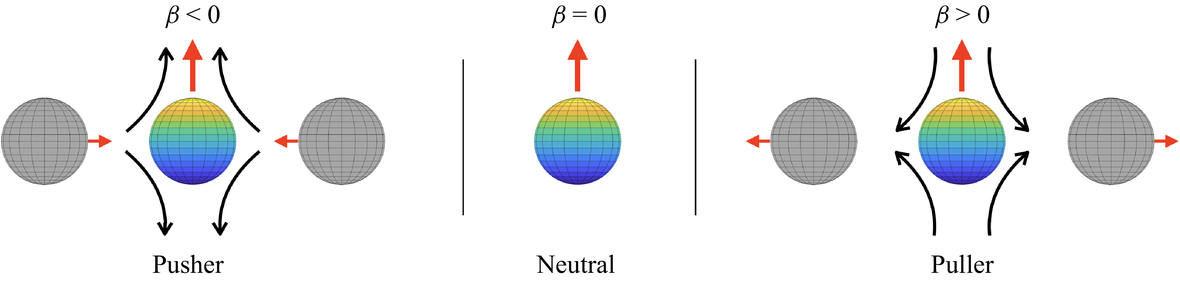

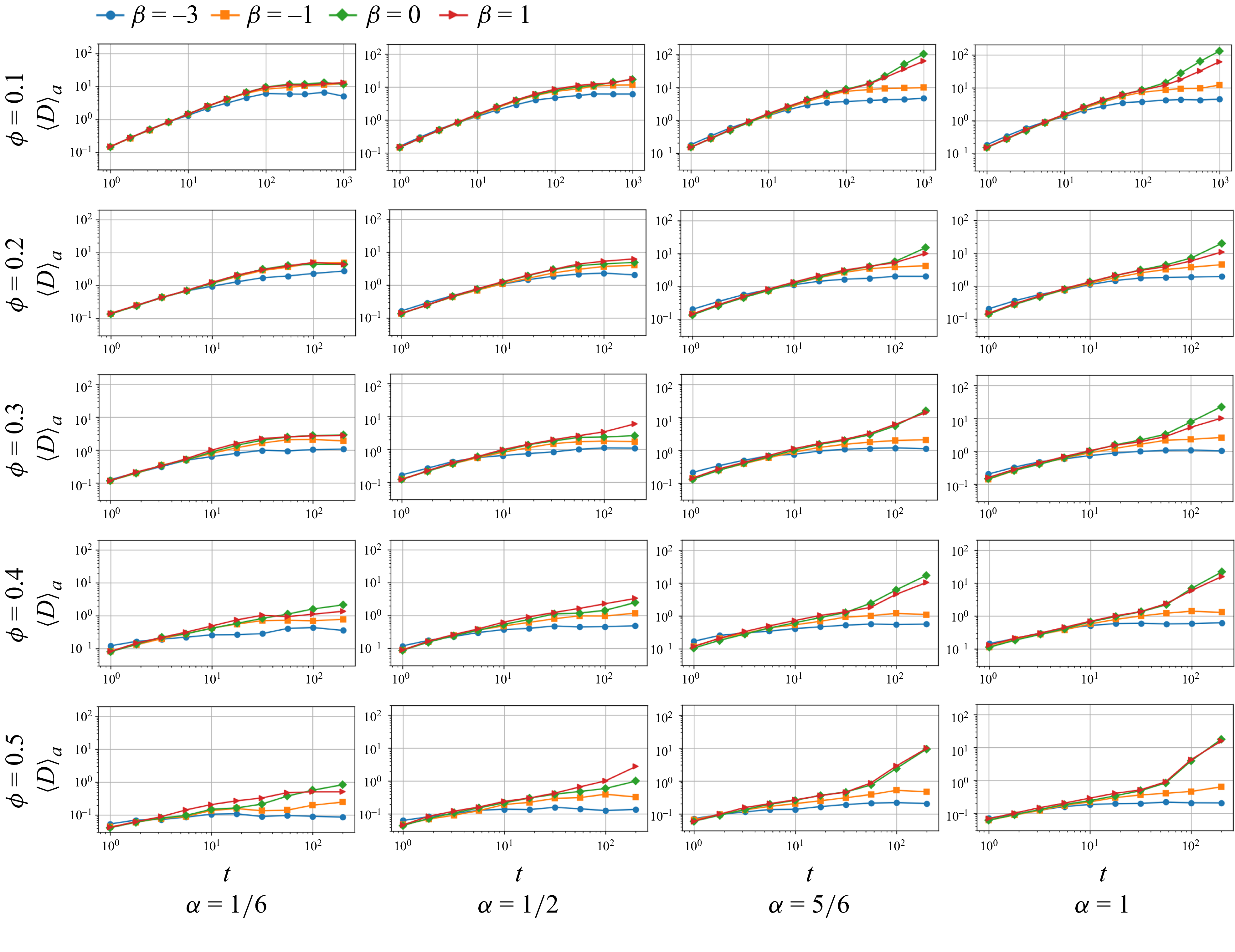


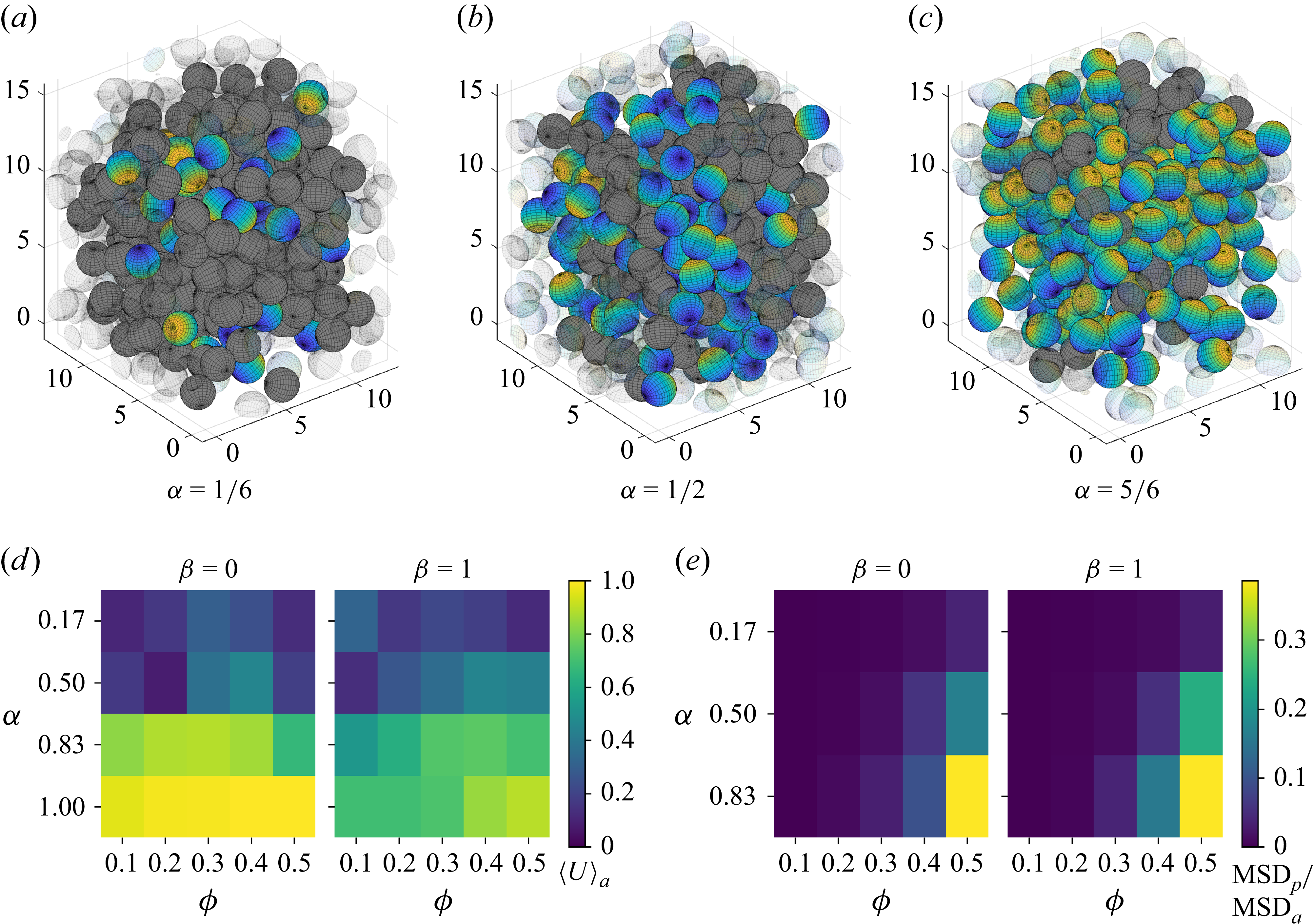


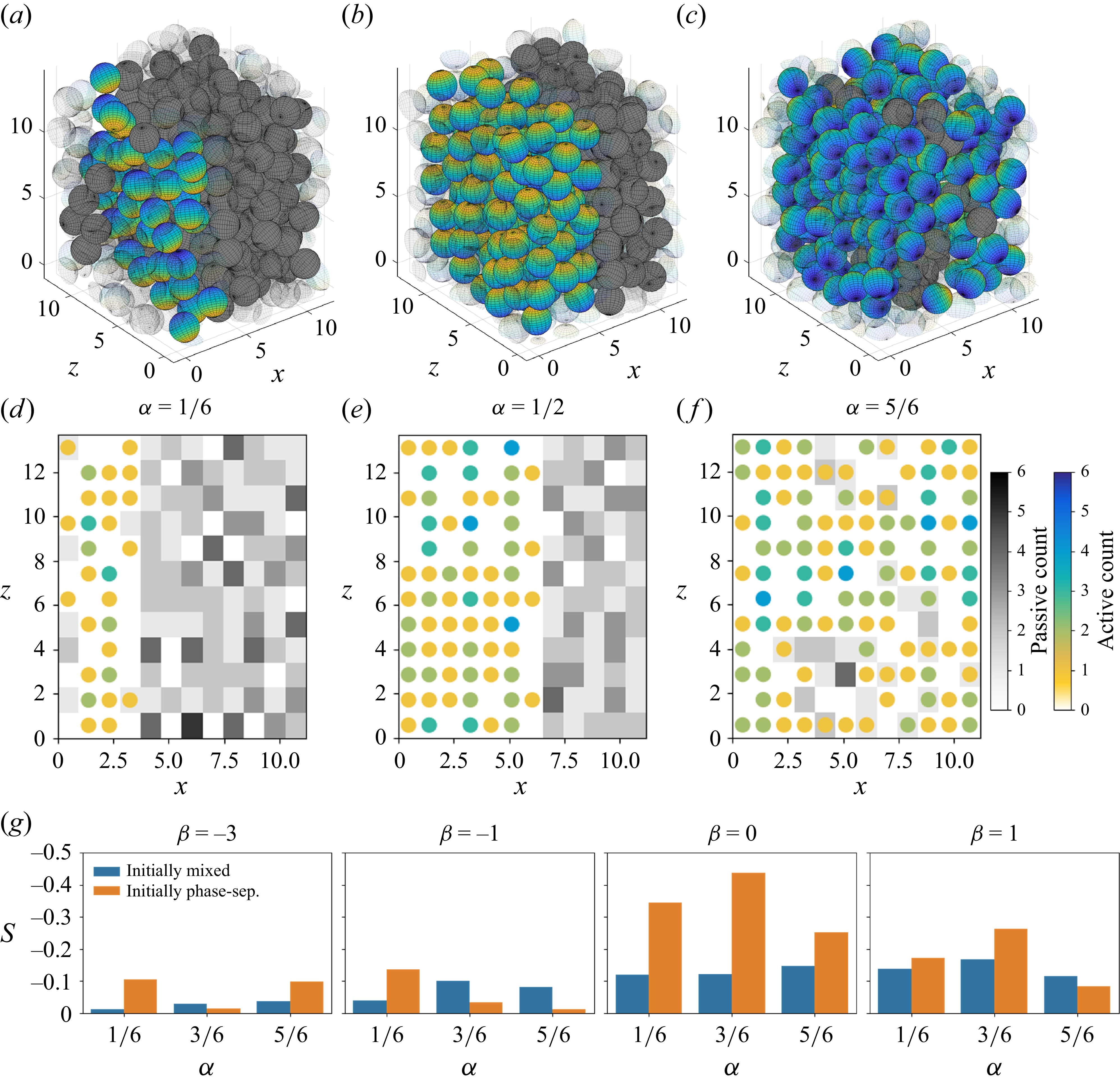


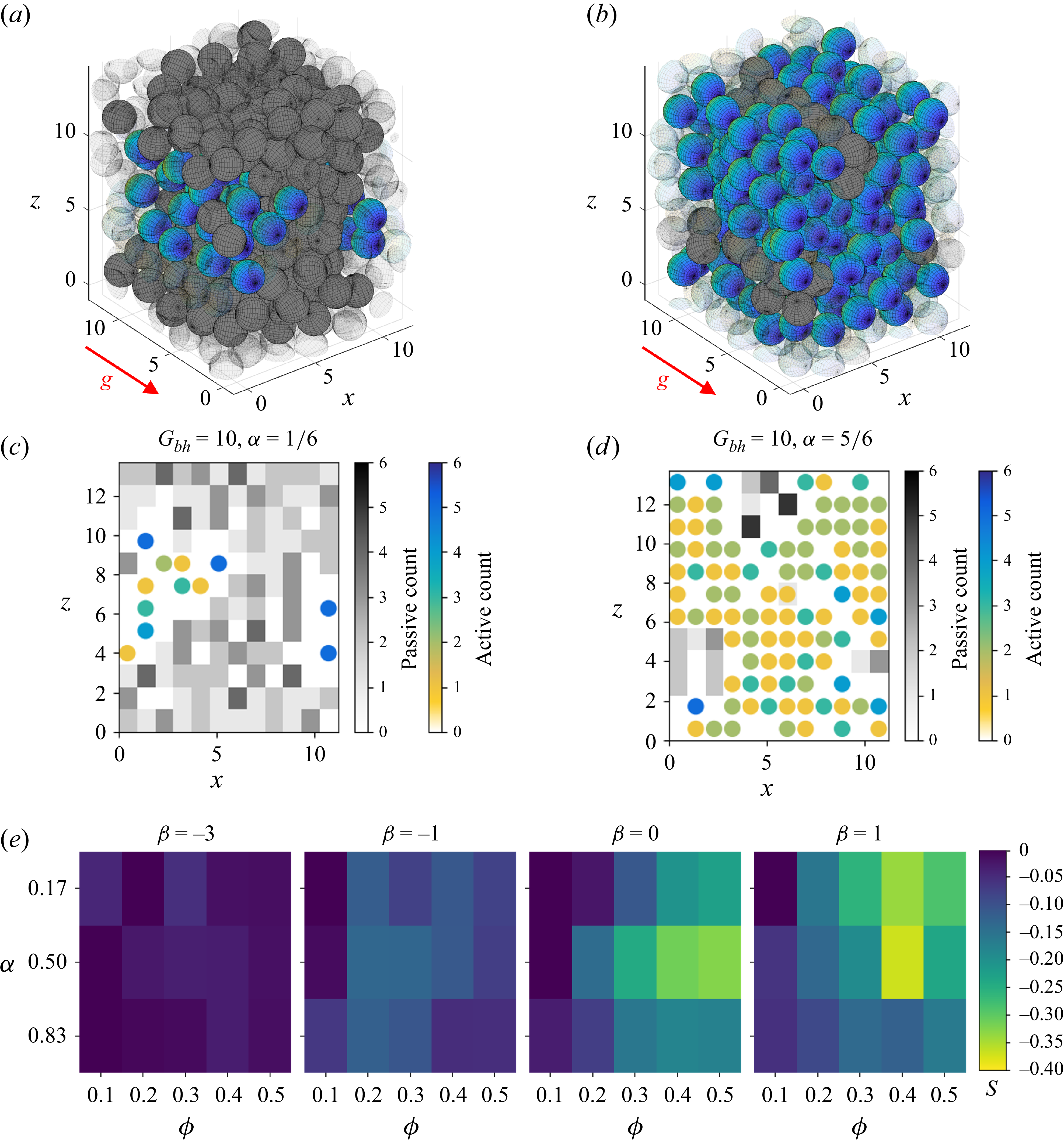


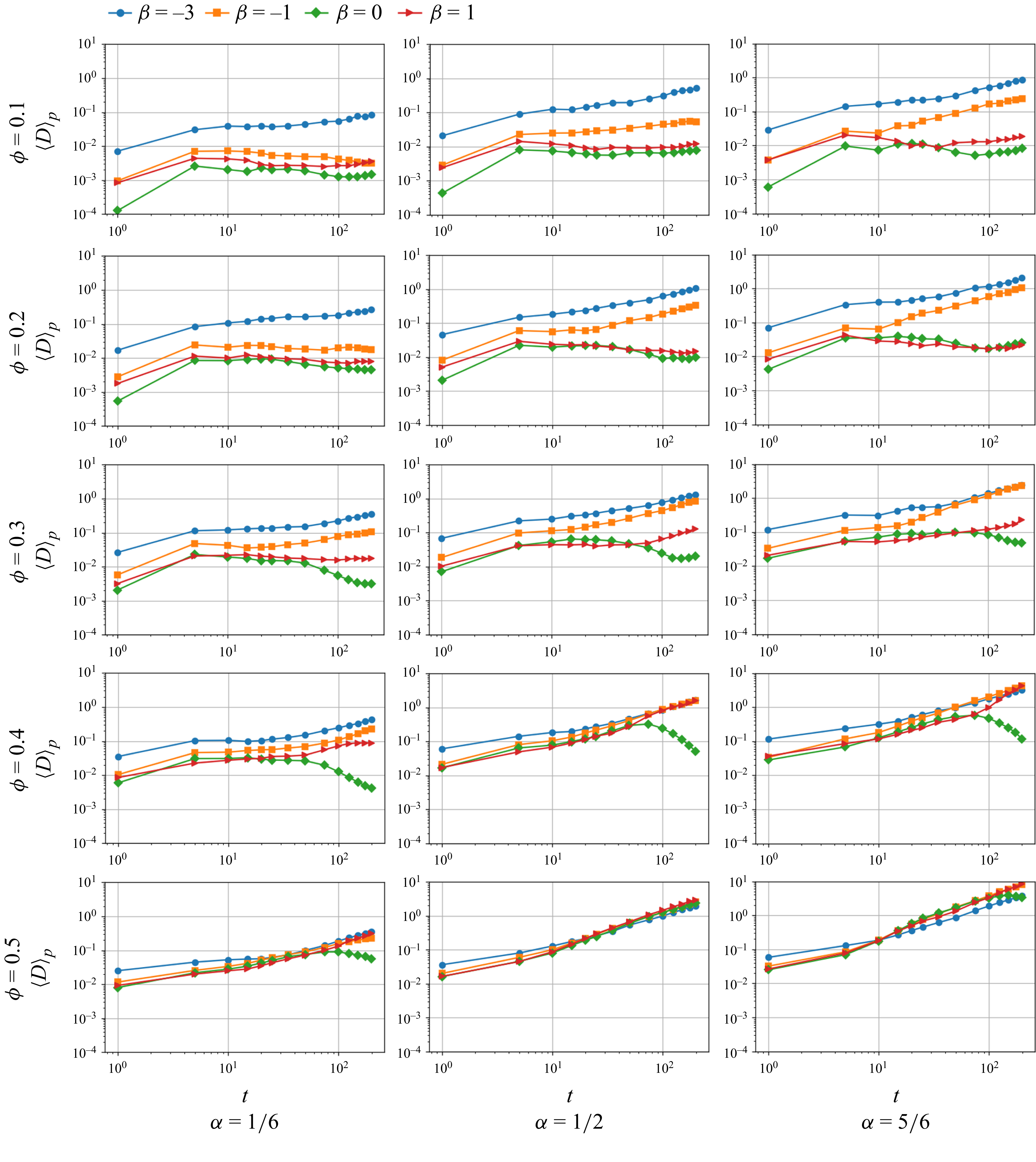


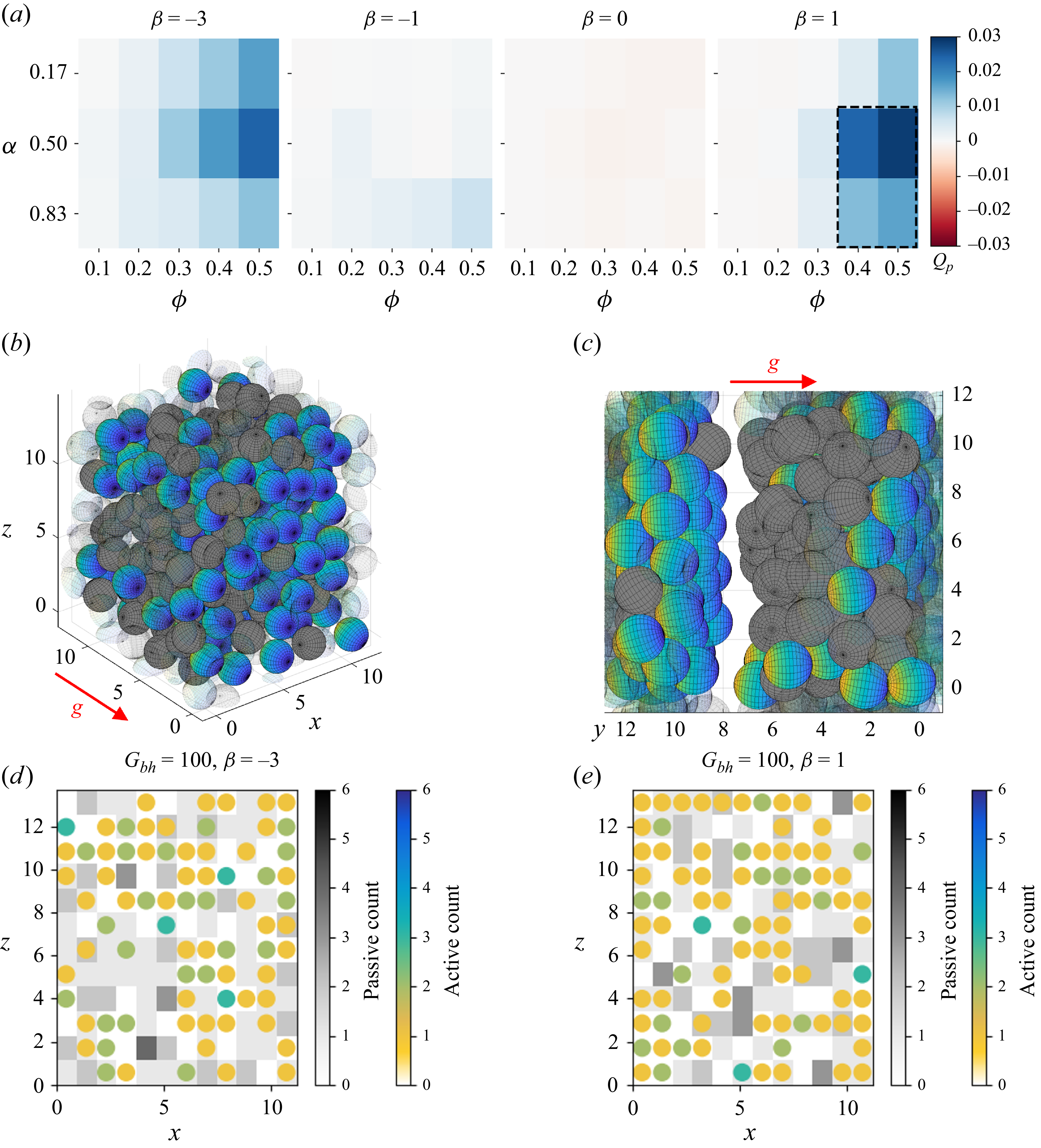


 Open access