





1. Introduction
In many flows, such as those past aeroplanes, ships or through pipelines, viscous drag is the primary factor that limits speed and efficiency. It has been suggested that as much as 50 %–60 % of the total drag experienced by cruising aircraft can be attributed to viscous drag (Ricco, Skote & Leschziner Reference Ricco, Skote and Leschziner2021). As a consequence, it is clear that in these types of flows a significant fraction of energy is spent overcoming the drag. Even a relatively modest reduction in drag could yield significant performance and economic benefits. It is, therefore, unsurprising that considerable effort has been devoted to developing flow control strategies that might reduce energy expenditure through viscous drag reduction. Most of this work has focused on turbulent flows, with a relative paucity of results discussing laminar flows. The present work focuses on laminar flow, although it is instructive to review strategies that have been developed in the context of turbulent flows.
Several strategies have been suggested in the pursuit of drag reduction. The various techniques can be divided into two broad categories: passive and active control. Passive approaches – which do not require energy input – include methods such as surface texturing (e.g. riblets) or using superhydrophobic, liquid-infused, porous, flexible or metamaterial surfaces. Active approaches – which do rely on an energy input – can be divided into four further sub-categories: fluidic, moving surface, plasma and field driven (Cattafesta & Sheplak Reference Cattafesta and Sheplak2011). Field-driven actuators include electromagnetic, magnetohydrodynamic, thermal (Yeh, Munday & Taira Reference Yeh, Munday and Taira2017) and (thermo)acoustic (Juniper Reference Juniper2011) mechanisms. Detailed overviews and discussions of active flow control approaches can be found in any of Bushnell & McGinley (Reference Bushnell and McGinley1989), Gad-el Hak (1989, 1996, 2000), Bushnell & Moore (Reference Bushnell and Moore1991), Brunton & Noack (Reference Brunton and Noack2015), Cattafesta & Sheplak (Reference Cattafesta and Sheplak2011), Yeh et al. (Reference Yeh, Munday and Taira2017), Juniper (Reference Juniper2011) and Choi, Moin & Kim (Reference Choi, Moin and Kim1994).
A common theme among many of these strategies is that they effectively modify the boundary condition at the surface. A large number of studies have investigated how directly modifying the wall-normal component of the velocity (often referred to as suction/blowing or transpiration) or the in-plane component perpendicular to the main flow direction (often referred to as spanwise wall motion) affects the skin friction.
The use of suction/blowing for flow control is a very well-developed research area. The particular technique of opposition control, which can achieve as much as 25 % drag reduction in a turbulent channel flow at a low Reynolds number, serves as a benchmark against which other techniques can be assessed (Choi et al. Reference Choi, Moin and Kim1994). For opposition control, the power required for actuation is reportedly negligible compared with the power saved due to drag reduction. Suction/blowing-based control has advanced to the point where optimised spatio-temporal patterns, based on control theory, have been developed and applied to turbulent channel flow (Bewley, Moin & Temam Reference Bewley, Moin and Temam2001). Furthermore, sustained sub-laminar levels of drag have been achieved in channel flow (Min et al. Reference Min, Kang, Speyer and Kim2006). Recent efforts using reinforcement learning have been able to achieve even greater levels of drag reduction in turbulent channel flow using strong actuation (e.g. Sonoda et al. Reference Sonoda, Liu, Itoh and Hasegawa2023).
Wall motions normal to the mean wall position are analogous to suction/blowing; they constitute another route for active flow control and might also be regarded as surface vibrations. This mechanism relies on the peristaltic effect, which pumps the fluid in the direction of propagation of the surface wave (Floryan et al Reference Floryan, Faisal and Panday2021), thereby reducing pressure losses. This form of work was first considered by Hoepffner & Fukagata (Reference Hoepffner and Fukagata2009), with more recent results on turbulent channel flow (Nabae et al. Reference Nabae, Inagaki, Kobayashi, Gotoda and Fukagata2025) and turbulent boundary layer (Albers, Shao & Schröder Reference Albers, Shao and Schröder2024; Yoshida et al. Reference Yoshida, Nimura, Mitsuishi, Murata and Iwamoto2025) confirming this expectation. Such vibrations can relaminarise a turbulent channel flow, which therefore constitutes a viable alternative mechanism for achieving drag reduction (Nakanishi, Hiroya Mamori & Fukagata Reference Nakanishi, Hiroya Mamori and Fukagata2012).
Another class of control involves using spanwise wall motion. Two recent reviews provide accounts of progress in this area (Ricco et al. Reference Ricco, Skote and Leschziner2021; Luchini & Quadrio Reference Luchini and Quadrio2022). Initial studies of this type of control considered uniform oscillations of the entire wall. These oscillations proved capable of reducing turbulent skin friction drag by up to 40 %–50 %, but were far less effective in reducing the net energy costs (Jung, Mangiavacchi & Akhavan Reference Jung, Mangiavacchi and Akhavan1992; Baron & Quadrio Reference Baron and Quadrio1995). This led to the investigation of spatio-temporal oscillations of the spanwise wall velocity, which take the form of streamwise-travelling waves, the current paradigm. Similarly, large drag reduction is possible, and the energy efficiency is generally improved. Recent work at large friction Reynolds numbers of ${\textit{Re}}_{\tau }=O(10^{4})$
has suggested net energy savings of perhaps 5 %–10 % (Marusic et al. Reference Marusic, Chandran, Rouhi, Fu, Wine, Holloway, Chung and Smits2021; Chandran et al. Reference Chandran, Zampiron, Rouhi, Fu, Wine, Holloway, Smits and Marusic2023), although these figures have been disputed (Gatti et al. Reference Gatti, Quadrio, Chiarini, Gatterre and Pirozzoli2025).
${\textit{Re}}_{\tau }=O(10^{4})$
has suggested net energy savings of perhaps 5 %–10 % (Marusic et al. Reference Marusic, Chandran, Rouhi, Fu, Wine, Holloway, Chung and Smits2021; Chandran et al. Reference Chandran, Zampiron, Rouhi, Fu, Wine, Holloway, Smits and Marusic2023), although these figures have been disputed (Gatti et al. Reference Gatti, Quadrio, Chiarini, Gatterre and Pirozzoli2025).
It is thought that there is a limit to the net energy savings that can be achieved using active flow control. Several studies have investigated this issue for internal flows, including those described in Bewley (Reference Bewley2009), Fukagata, Sugiyama & Kasagi (Reference Fukagata, Sugiyama and Kasagi2009), Hoepffner & Fukagata (Reference Hoepffner and Fukagata2009), Lieu, Moarref & Jovanović (Reference Lieu, Moarref and Jovanović2010), Moarref & Jovanović (Reference Moarref and Jovanović2010) and Floryan (Reference Floryan2023). What has emerged is that, when using suction/blowing, the net energy expenditure is minimised by the uncontrolled, laminar flow, at least for pressure-driven flow (Bewley Reference Bewley2009; Fukagata et al. Reference Fukagata, Sugiyama and Kasagi2009). In other words, uncontrolled laminar flow is the most energy efficient. It represents a fundamental limit to the potential energy savings that can be achieved by controlling turbulent flow. Similar conclusions can be drawn for shear-driven and combined pressure- and shear-driven flows, as well as for flows subject to spanwise wall motion (Floryan Reference Floryan2023). These energy efficiency limits present an obstacle to the prospect of ever-increasing savings via improved flow control (Luchini & Quadrio Reference Luchini and Quadrio2022; Kim Reference Kim2011; Jovanović Reference Jovanović2021; Fukagata, Iwamoto & Hasegawa Reference Fukagata, Iwamoto and Hasegawa2024). It should also be emphasised that the control of internal and external flows is somewhat different in character.
1.1. Control of laminar flows
The understanding of control and drag reduction strategies for laminar flows is arguably less developed, mainly because it has been widely believed that reducing laminar drag is not possible (Choi, Moin & Kim Reference Choi, Moin and Kim1991). The consideration of laminar flows introduces additional control objectives, including the intensification of mixing and the exploration of possible alternative propulsion methods. Passive methods based on properly structured surface grooves have demonstrated the potential for significant reduction in the frictional drag (Moradi & Floryan Reference Moradi and Floryan2013, Reference Moradi and Floryan2016; Mohammadi & Floryan Reference Mohammadi and Floryan2013a , Reference Mohammadi and Floryan2014, Reference Mohammadi and Floryan2015), especially when the groove shapes are optimised (Mohammadi & Floryan Reference Mohammadi and Floryan2013b ). Carefully selected grooves generate instabilities that promote flow mixing (Moradi & Floryan Reference Moradi and Floryan2014, Reference Moradi and Floryan2017, Reference Moradi and Floryan2019; Mohammadi, Moradi & Floryan Reference Mohammadi, Moradi and Floryan2015) and can produce chaotic mixing at low Reynolds numbers while simultaneously reducing the frictional losses (Gepner & Floryan Reference Gepner and Floryan2020).
Active methods for laminar flows often involve the use of heating patterns, heated grooves, thermal waves or surface vibrations. Heating patterns are particularly effective at a small Reynolds number, where they can eliminate pressure losses both in horizontal slots (Hossain et al. Reference Hossain and Floryan2012; Floryan & Floryan Reference Floryan and Floryan2015; Hossain & Floryan Reference Hossain and Floryan2016; Inasawa, Taneda & Floryan Reference Inasawa, Taneda and Floryan2019) and inclined conduits (Floryan et al. Reference Floryan, Wang and Bassom2023a , Reference Floryan, Wang and Bassom2024a ). They can also reduce the flow resistance (Floryan, Shadman & Hossain Reference Floryan, Shadman and Hossain2018). Heated grooves have proven to be a very potent resistance-reducing tool, as they activate pattern interaction (Floryan & Inasawa Reference Floryan and Inasawa2021), thermal streaming (Floryan, Panday & Aman Reference Floryan, Panday and Aman2023b ) and thermal drift (Abtahi & Floryan Reference Abtahi and Floryan2017; Inasawa, Hara & Floryan Reference Inasawa, Hara and Floryan2021; Floryan, Wang & Bassom Reference Floryan, Wang and Bassom2024b ) effects. An extensive discussion of some of their uses has been provided in Hossain & Floryan (2021) and Floryan et al. (Reference Floryan, Wang and Bassom2024), while a description of the propulsive effect can be found in Floryan, Aman & Panday (Reference Floryan, Aman and Panday2024c ). An interesting alternative option is offered by thermal waves, which can generate pumping (Hossain & Floryan Reference Hossain and Floryan2023) and propulsive (Hossain & Floryan Reference Hossain and Floryan2024a ) effects while also reducing flow losses (Hossain & Floryan Reference Hossain and Floryan2024b ). Heating patterns can also be used to generate low-Reynolds-number instabilities, thereby enhancing mixing (Panday & Floryan Reference Panday and Floryan2024). A separate group of active methods relies on surface vibrations, which create a propulsive effect (Haq & Floryan Reference Haq and Floryan2022, Reference Haq and Floryan2023). These vibrations take the form of waves, which can travel with or against the flow and may either increase or decrease the flow losses (Hoepffner & Fukagata Reference Hoepffner and Fukagata2009; Floryan & Haq Reference Floryan and Haq2022, Reference Floryan, Haq and Bassom2023d ; Haq & Floryan Reference Haq and Floryan2023). The role played by vibrations in intensifying mixing represents a separate direction of investigation (Floryan & Zandi Reference Floryan and Zandi2019; Haq & Floryan Reference Haq and Floryan2025).
In this work we examine flow control from a somewhat different perspective. Energy is typically invested in overcoming friction, and the common thinking is that flow control must achieve net energy savings to be successful. This is not necessarily the case, as one must also consider the energy cost required to generate a pressure gradient that drives flow along a conduit. To focus this discussion, consider a flow driven through the channel by a pressure gradient created by a pump. Energy has to be invested to the pump, but only a fraction of this is useful owing to the intrinsic inefficiency of the pump. Plausibly, a similar performance might be achievable by using the energy to drive distributed propulsion along the channel walls using spatial patterns of actuation. This system might prove to be a more energetically efficient propulsion as it avoids pump inefficiencies. It is conceivable that some combination of the two systems, distributed propulsion and a pump, might facilitate a performance level that is cannot be achieved by either system individually. Actuations utilising suction, heating and vibration patterns, as reviewed above, could be used to create distributed propulsion.
The present analysis focuses on an evaluation of the potential of contraction/relaxation waves to create a pumping/propulsion effect in internal flows. This is inspired by the mechanism that ciliated swimmers use to propel themselves, as well as how this mechanism is modelled in theoretical work (Ishikawa, Reference Ishikawa2024). Our interest lies in the use of spatial patterns of relatively weak waves rather than large magnitude waves. The analysis is therefore limited to small wave amplitudes but covers the complete range of wavenumbers and wave speeds. Moreover our interest is limited to Reynolds number for which the flow remains laminar. To address these questions, we organise the remainder of the work as follows. In § 2 we describe the model problem while § 3 outlines the computational solution method used. The subsequent sections are devoted to various aspects of the resulting flow. Section 4 focuses on the pumping effect generated by the waves while § 5 addresses how the waves impact pressure losses. Section 6 explores potential resonances between the waves and the natural frequencies of the flow, while § 7 demonstrates the generation of a propulsive effect. Analytical solutions can be obtained in various limits; they are derived in the appendices and referenced throughout the text. A summary and concluding remarks are presented in § 8.
2. Formulation
Consider the steady, two-dimensional flow of a fluid confined in a channel bounded by two parallel walls that are unbounded in the $X$
-direction. The plates are placed
$X$
-direction. The plates are placed $2h$
apart, and the flow is driven in the positive
$2h$
apart, and the flow is driven in the positive $X$
-direction by a constant pressure gradient. This generates velocity and pressure fields given by
$X$
-direction by a constant pressure gradient. This generates velocity and pressure fields given by
 \begin{equation}\boldsymbol{v}_{\mathbf{0}}\left(X,Y\right)=\big(1-Y^{2},0\big), p_{0}\left(X,Y\right)=-2X/{\textit{Re}}, {\varPsi _{0}}=Y-\frac{Y^{3}}{3}+\frac{2}{3}, Q_{0}=\frac{4}{3}.\end{equation}
Here, lengths have been expressed in terms of the channel half-width h and $\boldsymbol{v}_{\mathbf{0}}=(u_{0},v_{0})$
denotes the velocity vector scaled with the maximum of the
$\boldsymbol{v}_{\mathbf{0}}=(u_{0},v_{0})$
denotes the velocity vector scaled with the maximum of the $X$
-velocity
$X$
-velocity $u_{max}$
. The pressure
$u_{max}$
. The pressure $p_{0}$
is scaled on
$p_{0}$
is scaled on $\rho u_{max}^{2}$
, where
$\rho u_{max}^{2}$
, where $\rho$
is the fluid density,
$\rho$
is the fluid density, $\varPsi _{0}$
is the streamfunction and
$\varPsi _{0}$
is the streamfunction and $Q_{0}$
denotes the flow rate. Finally, the Reynolds number is defined as
$Q_{0}$
denotes the flow rate. Finally, the Reynolds number is defined as ${\textit{Re}}=u_{max}h/\nu$
, where
${\textit{Re}}=u_{max}h/\nu$
, where $\nu$
is the kinematic viscosity.
$\nu$
is the kinematic viscosity.
The flow is modified by imposing in-plane contraction/relaxation waves with prescribed amplitudes at the bounding walls, resulting in the boundary conditions
 \begin{align} Y& = 1 \colon \quad u_{U }\left(t,X\right)=\frac{1}{2}A_{U} \cos \left[\alpha \left(X-ct\right)+\varOmega \right]\!, \quad v_{U }\left(t,X\right)=0, \end{align}
 \begin{align} Y& = -1 \colon \quad u_{L }\left(t,X\right)= \frac{1}{2}A_{L} \cos \left[\alpha \left(X-ct\right)\right]\!,\quad v_{L }\left(t,X\right)=0, \end{align}
where $(u,v)$
are the
$(u,v)$
are the $(X,Y)$
components of the velocity vector scaled on the viscous velocity scale
$(X,Y)$
components of the velocity vector scaled on the viscous velocity scale $U_{v}=\nu /h$
,
$U_{v}=\nu /h$
, $A$
is the wave amplitude, the subscripts U and L refer to the upper and lower walls, respectively,
$A$
is the wave amplitude, the subscripts U and L refer to the upper and lower walls, respectively, $\alpha$
is the wavenumber, c denotes the phase speed,
$\alpha$
is the wavenumber, c denotes the phase speed, $ h/U_{v}$
is adopted as the time scale and
$ h/U_{v}$
is adopted as the time scale and $\varOmega$
is the phase difference between the upper and lower waves. Waves that travel in the flow direction have
$\varOmega$
is the phase difference between the upper and lower waves. Waves that travel in the flow direction have $c\gt 0$
, while waves that propagate against the flow have
$c\gt 0$
, while waves that propagate against the flow have $c\lt 0.$
A schematic of the flow geometry is shown in figure 1.
$c\lt 0.$
A schematic of the flow geometry is shown in figure 1.
A sketch of the flow configuration. The arrows represent the streamwise velocity (contraction/relaxation waves) at the lower and upper walls. The walls themselves are flat.

The flow is written as a sum of the reference flow and the wave-induced modifications
 \begin{align} u(t,X,Y)& = {\textit{Re}}\, u_{0}(Y)+u_{1}(t,X,Y), \qquad \quad\, v(t,X,Y)=v_{1}(t,X,Y),\\[-24pt]\nonumber \end{align}
 \begin{align} p(t,X,Y)& = {\textit{Re}}^{2}p_{0}(X)-B_{\textit{mod}}X+p_{1}(t,X,Y), \quad \psi (t,X,Y)={\textit{Re}} \psi _{0}(Y)+\psi _{1}(t,X,Y). \end{align}
Here, $(u_{1},v_{1})$
and
$(u_{1},v_{1})$
and $\psi _{1}$
denote the velocity and streamfunction modifications, respectively, while
$\psi _{1}$
denote the velocity and streamfunction modifications, respectively, while $ B_{\textit{mod}}$
represents the pressure-gradient correction and
$ B_{\textit{mod}}$
represents the pressure-gradient correction and $p_{1}$
denotes the periodic part of the pressure field modifications, both scaled with
$p_{1}$
denotes the periodic part of the pressure field modifications, both scaled with $\rho U_{v}^{2}$
as the pressure scale. Note that negative values of
$\rho U_{v}^{2}$
as the pressure scale. Note that negative values of $B_{\textit{mod}}$
correspond to a reduction of pressure losses, i.e. a reduced pressure gradient required to drive the flow.
$B_{\textit{mod}}$
correspond to a reduction of pressure losses, i.e. a reduced pressure gradient required to drive the flow.
Substituting (2.3) into the Navier–Stokes and continuity equations leads to the field equations for the flow modifications
 \begin{align} & \frac{\partial u_{1}}{\partial t}+\left({\textit{Re}}\, u_{0}+u_{1}\right)\frac{\partial u_{1}}{\partial X}+{\textit{Re}} v_{1}\frac{\textrm{d}u_{0}}{\textrm{d}Y}+v_{1}\frac{\partial u_{1}}{\partial Y} =B_{\textit{mod}}-\frac{\partial p_{1}}{\partial X}+\frac{\partial ^{2}u_{1}}{\partial X^{2}}+\frac{\partial ^{2}u_{1}}{\partial Y^{2}}, \\[-12pt]\nonumber \end{align}
 \begin{align}& \frac{\partial v_{1}}{\partial t}+\left({\textit{Re}}\, u_{0}+u_{1}\right)\frac{\partial v_{1}}{\partial X}+v_{1}\frac{\partial v_{1}}{\partial Y} =-\frac{\partial p_{1}}{\partial Y}+\frac{\partial ^{2}v_{1}}{\partial X^{2}}+\frac{\partial ^{2}v_{1}}{\partial Y^{2}},\\[-12pt]\nonumber \end{align}
 \begin{align}& \frac{\partial u_{1}}{\partial X}+\frac{\partial v_{1}}{\partial Y} =0, \end{align}
subject to the boundary conditions
 \begin{align} u_{1}\left(t, X, 1\right)& = \frac{1}{2}A_{U} \cos \left[\alpha \left(X-ct\right)+\varOmega \right]\!, v_{1} \left(t, X, 1\right)=0, \\[-12pt]\nonumber \end{align}
 \begin{align} u_{1} \left(t, X, -1\right)& = \frac{1}{2}A_{L} \cos \left[\alpha \left(X-ct\right)\right]\!, v_{1} \left(t, X, -1\right)=0. \end{align}
We aim to investigate whether surface waves can reduce the pressure gradient necessary to maintain the specified flow rate. Accordingly, we impose the mass flow rate constraint
 \begin{equation}Q=\left.Q\left(t,X\right)\right| _{\textit{mean}}=\left.\left(\int _{-1}^{1}u\left(t, X, Y\right){\rm d}Y\right)\right| _{\textit{mean}}=\frac{4}{3}{\textit{Re}},\end{equation}
where the subscript `mean’ refers to the average taken over one period.
A complete description of the flow mechanics requires knowledge of the surface forces acting on the fluid at the walls. The components of the stress are
 \begin{align} Y& = -1\colon \sigma _{X,L}=-\left(\frac{\partial u}{\partial Y}+\frac{\partial v_{1}}{\partial X}\right)\!,\sigma _{Y,L}=-2\frac{\partial v_{1}}{\partial Y}+p, \end{align}
 \begin{align} Y& = 1\colon \sigma _{X,U}=\frac{\partial u}{\partial Y}+\frac{\partial v_{1}}{\partial X},\sigma _{Y,U}=2\frac{\partial v_{1}}{\partial Y} -p, \end{align}
where $(\sigma _{X},\sigma _{Y})$
denote the
$(\sigma _{X},\sigma _{Y})$
denote the $(X,Y)$
-components. The X- and Y-components of the total force
$(X,Y)$
-components. The X- and Y-components of the total force $(F_{X,L}, F_{Y,L})$
(per unit length and width of the channel) are
$(F_{X,L}, F_{Y,L})$
(per unit length and width of the channel) are
 \begin{align} Y & =-1\colon F_{X,L}=-\lambda ^{-1}\int _{X_{0}}^{X_{0}+\lambda }\left(\frac{\partial u}{\partial Y}+\frac{\partial v_{1}}{\partial X}\right){\rm d}X, \nonumber \\F_{Y,L}& =F_{Yv,L}+F_{Yp,L} =-2\lambda ^{-1}\int _{X_{0}}^{X_{0}+\lambda }\frac{\partial v_{1}}{\partial Y}{\rm d}X+\lambda ^{-1}\int _{X_{0}}^{X_{0}+\lambda }p {\rm d}X, \\[-12pt]\nonumber \end{align}
 \begin{align} Y& =1\colon F_{X,U}=\lambda ^{-1}\int _{X_{0}}^{X_{0}+\lambda }\left(\frac{\partial u}{\partial Y}+\frac{\partial v_{1}}{\partial X}\right){\rm d}X, \nonumber \\F_{Y,U} &=\lambda ^{-1}\int _{X_{0}}^{X_{0}+\lambda }2\frac{\partial v_{1}}{\partial Y}{\rm d}X-\lambda ^{-1}\int _{X_{0}}^{X_{0}+\lambda }p {\rm d}X, \end{align}
where $X_{0}$
is a convenient reference point. The wave-induced changes of surface forces are
$X_{0}$
is a convenient reference point. The wave-induced changes of surface forces are
 \begin{equation}{\unicode[Arial]{x0394}} F_{X,U}=F_{X,U}+2{\textit{Re}},{\unicode[Arial]{x0394}} F_{X,L}=F_{X,L}+2Re.\end{equation}
The final quantity of interest is the force created by the mean pressure gradient $F_{Xp,m}=\left.({\partial p}/{\partial X})\right| _{\textit{mean}}$
per unit length and unit width of the channel. Its change due to vibrations is defined as
$F_{Xp,m}=\left.({\partial p}/{\partial X})\right| _{\textit{mean}}$
per unit length and unit width of the channel. Its change due to vibrations is defined as
 \begin{equation}{\unicode[Arial]{x0394}} F_{Xpm}=2\left(\left.\frac{\partial p}{\partial X}\right| _{\textit{mean}}-{\textit{Re}}^{2}\frac{{\rm d}p_{0}}{{\rm d}X}\right)=-2B_{\textit{mod}}.\end{equation}
3. The computational method
The analysis is simplified by introducing a frame of reference that moves at the same speed as the wave phase. A Galilean transformation of the form
 \begin{equation}y = Y, x = X - ct\end{equation}
leads to a steady problem
 \begin{align}\left({\textit{Re}}\, u_{0}+u_{1}-c\right)\frac{\partial u_{1}}{\partial x}+{\textit{Re}}\, v_{1}\frac{\text{d}u_{0}}{{\rm d}y}+v_{1}\frac{\partial u_{1}}{\partial y}& = B_{\textit{mod}}-\frac{\partial p_{1}}{\partial x}+\frac{\partial ^{2}u_{1}}{\partial x^{2}}+\frac{\partial ^{2}u_{1}}{\partial y^{2}},\end{align}
 \begin{align}\left({\textit{Re}}\, u_{0}+u_{1}-c\right)\frac{\partial v_{1}}{\partial x}+v_{1}\frac{\partial v_{1}}{\partial y}& = -\frac{\partial p_{1}}{\partial y}+\frac{\partial ^{2}v_{1}}{\partial x^{2}}+\frac{\partial ^{2}v_{1}}{\partial y^{2}}, \end{align}
 \begin{align}\frac{\partial u_{1}}{\partial x}+\frac{\partial v_{1}}{\partial y}& = 0,\end{align}
subject to the boundary conditions
 \begin{align}y& = 1\colon \qquad u_{1}=\frac{1}{2}A_{U} \cos \left(\alpha x+\varOmega \right)\!, \quad v_{1}=0, \end{align}
 \begin{align}y& = -1\colon \quad u_{1}=\frac{1}{2}A_{L} \cos \left(\alpha x\right)\!, \qquad \quad\,\, v_{1} =0 \end{align}
and
 \begin{equation}Q=\left.\left\{\int _{-1}^{1}\left[{\textit{Re}}\, u_{0}(y)+u_{1}\left(x,y\right)\right]{\rm d}y\right\}\right| _{\textit{mean}}=\frac{4}{3}Re.\end{equation}
We begin by eliminating the pressure using the streamfunction modification $\psi _{1}$
. This leaves
$\psi _{1}$
. This leaves
 \begin{align}\boldsymbol{\nabla} ^{2}\big({\nabla} ^{2}\psi _{1}\big)-\left({\textit{Re}}\, u_{0}-c\right)\frac{\partial }{\partial x}{\nabla} ^{2}\psi _{1}+Re\frac{{{\rm d}^{2}}u_{0}}{{\rm d}y^{2}}\frac{\partial \psi _{1}}{\partial x}& = \frac{\partial }{\partial y}\left(\frac{\partial }{\partial x}(u_{1}u_{1})+\frac{\partial }{\partial y}(u_{1}v_{1})\right)\nonumber\\ & \quad -\frac{\partial }{\partial x}\left(\frac{\partial }{\partial x}(u_{1}v_{1})+\frac{\partial }{\partial y}(v_{1}v_{1})\right)\!,\end{align}
with
 \begin{align}y& = 1\colon \qquad \frac{\partial \psi _{1}}{\partial y}=\frac{1}{2}A_{U}\cos \left(\alpha x+\varOmega \right)\!, \quad \psi _{1}= 0, \end{align}
 \begin{align}y& = -1\colon \quad\, \frac{\partial \psi _{1}}{\partial y}=\frac{1}{2}A_{L} \cos \left(\alpha x\right)\!, \qquad \quad\, \psi _{1}=0, \end{align}
which accounts for the flow rate constraint (3.2f ).
Since the waves are periodic, all unknowns can be expressed as Fourier expansions of the form
 \begin{equation}q_{1}\left(x,y\right)=\sum \nolimits_{m=-N_{M}}^{m=+N_{M}}q_{1}^{\left(m\right)}(y)e^{im\alpha x},\end{equation}
where $q_{1}$
represents any of
$q_{1}$
represents any of $\psi _{1}, v_{1}, u_{1},p_{1}$
or the products
$\psi _{1}, v_{1}, u_{1},p_{1}$
or the products $u_{1}u_{1}, u_{1}v_{1}$
and
$u_{1}u_{1}, u_{1}v_{1}$
and $v_{1}v_{1}$
. The modal functions
$v_{1}v_{1}$
. The modal functions $q_{1}^{(m)}$
necessarily satisfy appropriate reality conditions so that
$q_{1}^{(m)}$
necessarily satisfy appropriate reality conditions so that $q_{1}^{(m)}$
must necessarily be the complex conjugate of
$q_{1}^{(m)}$
must necessarily be the complex conjugate of $q_{1}^{(-m)}$
. The resulting system of nonlinear differential equations for the modal functions is
$q_{1}^{(-m)}$
. The resulting system of nonlinear differential equations for the modal functions is
 \begin{align}& \left\{D^{4}+\big[-2m^{2}\alpha ^{2}-im\alpha \left({\textit{Re}}\, u_{0}-c\right)\big]D^{2}+\big[m^{4}\alpha ^{4}+im^{3}\alpha ^{3}\left({\textit{Re}}\, u_{0}-c\right)\big]\right.\nonumber\\& \left . +\,im\alpha\, {\textit{ReD}}^{2}u_{0}\right\}{\varphi _{1}}^{\left(m\right)}=im\alpha D \left\{u_{1}u_{1}\right\}^{(m)}\!+\big[\!D^{2}+\left(m\alpha \right)^{2}\big]\left\{u_{1}v_{1}\right\}^{\left(m\right)} -im\alpha D \left\{v_{1}v_{1}\right\}^{\left(m\right)}\!,\end{align}
where $D\equiv ({\rm d}/{{\rm d}y})$
and
$D\equiv ({\rm d}/{{\rm d}y})$
and $-N_{M}\leq m\leq N_{M}$
. The system is solved iteratively, with the nonlinear terms on the right-hand side calculated based on the results of the previous iteration. This means that a system of linear inhomogeneous differential equations has to be solved at each iteration. The various modal functions
$-N_{M}\leq m\leq N_{M}$
. The system is solved iteratively, with the nonlinear terms on the right-hand side calculated based on the results of the previous iteration. This means that a system of linear inhomogeneous differential equations has to be solved at each iteration. The various modal functions $q_{1}^{(m)}(y)$
were expressed as Chebyshev expansions, and linear algebraic equations for their coefficients were constructed using the Galerkin projection method with the boundary conditions implemented using the tau concept (Canuto et al. 2006). The pressure-gradient correction
$q_{1}^{(m)}(y)$
were expressed as Chebyshev expansions, and linear algebraic equations for their coefficients were constructed using the Galerkin projection method with the boundary conditions implemented using the tau concept (Canuto et al. 2006). The pressure-gradient correction $B_{\textit{mod}}$
was found by substituting Fourier expansions for the unknowns into the streamwise momentum equation and then extracting the zeroth mode. Computations were carried out with a minimum of five-digit accuracy, which dictated the number of Fourier modes and the number of Chebyshev polynomials to be used. One advantage of the algorithm is that it provides access to machine accuracy when needed.
$B_{\textit{mod}}$
was found by substituting Fourier expansions for the unknowns into the streamwise momentum equation and then extracting the zeroth mode. Computations were carried out with a minimum of five-digit accuracy, which dictated the number of Fourier modes and the number of Chebyshev polynomials to be used. One advantage of the algorithm is that it provides access to machine accuracy when needed.
4. The pumping effect
Our discussion begins by demonstrating how in-plane contraction/relaxation waves can create a pumping effect. To do so, we set ${\textit{Re}}=0$
(which sets the base Poiseuille flow to zero) and ascertain the flow rate produced by the waves in the absence of any longitudinal pressure gradient. This is deduced by replacing the constraint (2.4f
) with the fixed pressure-gradient specification
${\textit{Re}}=0$
(which sets the base Poiseuille flow to zero) and ascertain the flow rate produced by the waves in the absence of any longitudinal pressure gradient. This is deduced by replacing the constraint (2.4f
) with the fixed pressure-gradient specification
 \begin{equation}B_{\textit{mod}}=0.\end{equation}
As stated at the outset, our interest lies in laminar flow and an exploration of the most effective spatial patterns. The results displayed in figure 2 show the net flow rate $Q$
as a function of the wave amplitude
$Q$
as a function of the wave amplitude $A_{L}$
. It is evident that
$A_{L}$
. It is evident that $Q$
is very close to being proportional to
$Q$
is very close to being proportional to $A_{L}^{2}$
for relatively weak waves, by which we mean waves with
$A_{L}^{2}$
for relatively weak waves, by which we mean waves with $A_{L}\lt \sim 100$
. Any increase in the amplitude beyond this results in the progressive flow rate saturation and a slowdown in the rise of
$A_{L}\lt \sim 100$
. Any increase in the amplitude beyond this results in the progressive flow rate saturation and a slowdown in the rise of $Q$
with
$Q$
with $A_{L}$
, which reduces the effectiveness of energy expenditure associated with amplitude increase. The usefulness of the restriction to weak waves is that results can be discussed in terms of a normalised flow rate
$A_{L}$
, which reduces the effectiveness of energy expenditure associated with amplitude increase. The usefulness of the restriction to weak waves is that results can be discussed in terms of a normalised flow rate $Q_{\textit{norm}}=10^{4}Q/A_{L}^{2}$
whose value is almost independent of the precise wave amplitude.
$Q_{\textit{norm}}=10^{4}Q/A_{L}^{2}$
whose value is almost independent of the precise wave amplitude.
The variations of the flow rate $Q$
as a function of the wave amplitude
$Q$
as a function of the wave amplitude $A_{L}$
when
$A_{L}$
when $c=-25$
,
$c=-25$
, $\alpha =2.2$
and
$\alpha =2.2$
and $A_{U}=0$
.
$A_{U}=0$
.

The structure of $Q_{\textit{norm}}$
as a function of
$Q_{\textit{norm}}$
as a function of $\alpha$
and c is depicted in figure 3. We remind the reader that the viscous velocity scale was used to scale the wave speed. The direction of pumping is opposite to that of wave movement, and there is an optimal pair of values c and
$\alpha$
and c is depicted in figure 3. We remind the reader that the viscous velocity scale was used to scale the wave speed. The direction of pumping is opposite to that of wave movement, and there is an optimal pair of values c and $\alpha$
that maximises the induced flow rate Q. The flow rate drops off rapidly as the flow parameters change from this optimum.
$\alpha$
that maximises the induced flow rate Q. The flow rate drops off rapidly as the flow parameters change from this optimum.
The normalised flow rate $Q_{\textit{norm}}=10^{4}Q/A_{L}^{2}$
as a function of
$Q_{\textit{norm}}=10^{4}Q/A_{L}^{2}$
as a function of $\alpha$
and
$\alpha$
and $c$
when
$c$
when $A_{U}=0$
. The horizontal lines identify the conditions used in figure 7. Red dots identify the conditions used in figures 5 and 6. The vertical lines identify conditions used in figure 10, and green dots denote the conditions used in figures 8 and 9.
$A_{U}=0$
. The horizontal lines identify the conditions used in figure 7. Red dots identify the conditions used in figures 5 and 6. The vertical lines identify conditions used in figure 10, and green dots denote the conditions used in figures 8 and 9.

Next, we examine why a contraction/relaxation wave propagating in one direction generates a net flow in the opposite direction. In our coordinate system, the fluid is driven to the right along the bottom of the channel for $x\in (0,({\lambda }/{4}))$
and
$x\in (0,({\lambda }/{4}))$
and $x\in (({3\lambda }/{4}),\lambda )$
, and to the left for
$x\in (({3\lambda }/{4}),\lambda )$
, and to the left for $x\in (({\lambda }/{4}),({3\lambda }/{4}))$
; this forms two stagnation points, as illustrated in figure 4(a). The fluid approaches the left stagnation point and is forced to turn upward by a local pressure maximum. It is driven away from the right stagnation point along the wall, and the local pressure minimum draws fluid from the interior to fill the vacated space. The flow and pressure fields exhibit reflection symmetry with respect to the stagnation points when
$x\in (({\lambda }/{4}),({3\lambda }/{4}))$
; this forms two stagnation points, as illustrated in figure 4(a). The fluid approaches the left stagnation point and is forced to turn upward by a local pressure maximum. It is driven away from the right stagnation point along the wall, and the local pressure minimum draws fluid from the interior to fill the vacated space. The flow and pressure fields exhibit reflection symmetry with respect to the stagnation points when $c=0$
. The moving wave destroys this symmetry, as illustrated in figure 4(b). The left stagnation point propagates to the left, with the fluid behind it forming a wedge that forces the fluid on the left side of this point upwards. The local pressure maximum near the left stagnation point increases considerably above its reference value for
$c=0$
. The moving wave destroys this symmetry, as illustrated in figure 4(b). The left stagnation point propagates to the left, with the fluid behind it forming a wedge that forces the fluid on the left side of this point upwards. The local pressure maximum near the left stagnation point increases considerably above its reference value for $c=0$
as the upward redirection of the fluid is more rapid. Similarly, the pressure minimum near the right stagnation point is also stronger than when
$c=0$
as the upward redirection of the fluid is more rapid. Similarly, the pressure minimum near the right stagnation point is also stronger than when $c=0$
as the fluid is drawn to the left more rapidly owing to the wave motion. The wave-generated upward (downward) forcing of the fluid near the left (right) stagnation point combines to give a net flow to the right.
$c=0$
as the fluid is drawn to the left more rapidly owing to the wave motion. The wave-generated upward (downward) forcing of the fluid near the left (right) stagnation point combines to give a net flow to the right.
The flow and pressure fields when $\alpha =1\ \mathrm{and}\ A_{U}=0$
for (a)
$\alpha =1\ \mathrm{and}\ A_{U}=0$
for (a) $c=0$
and (b)
$c=0$
and (b) $c=-25$
.
$c=-25$
.

The waves can generate a variety of flow topologies, which are displayed in figure 5. In general, the waves produce a system of counter-rotating rolls centred around the wave crests and troughs. The fluid moves to the right (left) above the wave crest (trough) near the actuated wall. Nonlinear streaming produces a net flow along the channel axis in the direction opposite to the wave movement. This forms a stream tube which gently meanders between the rolls. The overall flow topology in the case of long waves (figure 5
a) is reminiscent of a sloshing-type motion. By way of contrast, short waves create a boundary layer near the actuated wall and a uniform flow above it (figure 5
f), which we refer to as the wall regime. There is a gradual transition between these two behaviours, as illustrated in the sequence (figure 5
b–e). An increase in $\alpha$
shrinks the separation bubble next to the upper wall, which forms two roll centres, as apparent in figure 5(c). A further increase in
$\alpha$
shrinks the separation bubble next to the upper wall, which forms two roll centres, as apparent in figure 5(c). A further increase in $\alpha$
leads to the splitting of the upper separation bubble with a stream tube lying in between them, as shown in figure 5(d). A further increase in
$\alpha$
leads to the splitting of the upper separation bubble with a stream tube lying in between them, as shown in figure 5(d). A further increase in $\alpha$
sees the eventual elimination of the top separation bubble while the lower bubble morphs into an in-flow separation bubble (see figure 5
e). The topological structure shown in figure 4(e) persists but becomes confined within a boundary layer that forms near the wall, as illustrated in figure 5(f). In general, it seems that the width of the stream tube grows monotonically with
$\alpha$
sees the eventual elimination of the top separation bubble while the lower bubble morphs into an in-flow separation bubble (see figure 5
e). The topological structure shown in figure 4(e) persists but becomes confined within a boundary layer that forms near the wall, as illustrated in figure 5(f). In general, it seems that the width of the stream tube grows monotonically with $\alpha$
.
$\alpha$
.
The topology of wave-driven flows for $c=-25, A_{U}=0$
, and various values of the wavenumber
$c=-25, A_{U}=0$
, and various values of the wavenumber $\alpha$
. Panels show (a)
$\alpha$
. Panels show (a) $\alpha =0.1$
, (b)
$\alpha =0.1$
, (b) $\alpha =1$
, (c)
$\alpha =1$
, (c) $\alpha =1.5$
, (d)
$\alpha =1.5$
, (d) $\alpha =1.7$
, (e)
$\alpha =1.7$
, (e) $\alpha =2$
and ( f)
$\alpha =2$
and ( f) $\alpha =10$
. Separating streamlines are indicated by yellow lines, while stream tubes containing fluid moving to the right are denoted using green lines. The conditions used in (a), (b) and ( f) are marked with red dots in figure 3.
$\alpha =10$
. Separating streamlines are indicated by yellow lines, while stream tubes containing fluid moving to the right are denoted using green lines. The conditions used in (a), (b) and ( f) are marked with red dots in figure 3.

The evolution of the form of the flow field as $\alpha$
is changed is illustrated by the plots of
$\alpha$
is changed is illustrated by the plots of $u_{1}$
displayed in figure 6. We observe various distinctive behaviours. At a small wavenumber, there are significant variations of
$u_{1}$
displayed in figure 6. We observe various distinctive behaviours. At a small wavenumber, there are significant variations of $u_{1}$
as might be anticipated in a sloshing-type regime (figure 6
a). As
$u_{1}$
as might be anticipated in a sloshing-type regime (figure 6
a). As $\alpha$
increases, the velocities in the upper part of the channel begin to diminish (figure 6
b). When
$\alpha$
increases, the velocities in the upper part of the channel begin to diminish (figure 6
b). When $\alpha$
is large, almost all the wave-induced motion is confined to the boundary layer, with a rectilinear flow above (figure 6
c). The outer flow moves as if the edge of the boundary layer were a wall moving to the right and assumes a form similar to that of Couette flow.
$\alpha$
is large, almost all the wave-induced motion is confined to the boundary layer, with a rectilinear flow above (figure 6
c). The outer flow moves as if the edge of the boundary layer were a wall moving to the right and assumes a form similar to that of Couette flow.
The form of $u_{1}$
at the four streamwise locations
$u_{1}$
at the four streamwise locations $x/\lambda =0, 0.25, 0.5, 0.75$
when
$x/\lambda =0, 0.25, 0.5, 0.75$
when $c=-25, A_{L}=51\ \mathrm{and}\ A_{U}=0.$
Three wavenumbers are considered: (a)
$c=-25, A_{L}=51\ \mathrm{and}\ A_{U}=0.$
Three wavenumbers are considered: (a) $\alpha =0.1$
, (b)
$\alpha =0.1$
, (b) $\alpha =1$
and (c)
$\alpha =1$
and (c) $\alpha =10$
. The conditions used in these figures correspond to the points marked by red dots in figure 3.
$\alpha =10$
. The conditions used in these figures correspond to the points marked by red dots in figure 3.

The variation of the flow rate generated by waves as a function of wavenumber is illustrated in figure 7. The flow rate rapidly decreases as $\alpha \rightarrow 0$
with
$\alpha \rightarrow 0$
with
 \begin{equation}Q=-\frac{1}{4\, 15\, 800}\left\{ (99\,c-8\, \textit{Re})\big(A_{U}^{2}+A_{L}^{2}\big)-(16\textit{Re}+132c)A_{L}A_{U}\cos \varOmega \right\}\!\alpha ^{2}\!+O \big(\alpha ^{4}\big)\end{equation}
and also falls in the short-wavelength $\alpha \rightarrow \infty$
limit
$\alpha \rightarrow \infty$
limit
 \begin{equation}Q=-\frac{1}{128}c \big(A_{L}^{2}+A_{U}^{2}\big) \alpha ^{-2}+O\big(\alpha ^{-4}\big).\end{equation}
The flow rate $Q$
as a function of
$Q$
as a function of $\alpha$
when
$\alpha$
when $A_{L}=51$
and
$A_{L}=51$
and $ A_{U}=0$
Three values of the phase speed are shown:
$ A_{U}=0$
Three values of the phase speed are shown: $c=-25$
(blue line),
$c=-25$
(blue line), $c=-100$
(orange) and
$c=-100$
(orange) and $c=-500$
(yellow). The flow conditions used in this figure correspond to the blue, orange and yellow horizontal lines in figure 3.
$c=-500$
(yellow). The flow conditions used in this figure correspond to the blue, orange and yellow horizontal lines in figure 3.

Details of the corresponding asymptotic structures are described in Appendices A and B.
The flow structure changes only very slightly as the wave speed c is altered. Typical results are shown in figure 8. The flow assumes a sloshing-type structure, with the amplitude of the sloshing decreasing in the upper part of the channel as the phase speed increases, as shown in figure 9.
The topology of the wave-driven flow when $\alpha =1, A_{U}=0$
, and three wave speeds: (a)
$\alpha =1, A_{U}=0$
, and three wave speeds: (a) $c=-10$
, (b)
$c=-10$
, (b) $c=-100$
, (c)
$c=-100$
, (c) $c=-500$
. The separating streamlines are depicted by yellow lines, while stream tubes containing fluid moving to the right are shown by green lines. The conditions used in these figures are marked with green dots in figure 3.
$c=-500$
. The separating streamlines are depicted by yellow lines, while stream tubes containing fluid moving to the right are shown by green lines. The conditions used in these figures are marked with green dots in figure 3.

The distributions of $u_{1}$
at four streamwise stations
$u_{1}$
at four streamwise stations $x/\lambda =0,0.25,0.5,0.75$
when
$x/\lambda =0,0.25,0.5,0.75$
when $\alpha =1, A_{L}=51\ \mathrm{and}\ A_{U}=0.$
Three wave speeds are considered: (a)
$\alpha =1, A_{L}=51\ \mathrm{and}\ A_{U}=0.$
Three wave speeds are considered: (a) $c=-10$
, (b)
$c=-10$
, (b) $c=-100$
and (c)
$c=-100$
and (c) $c=-500$
. The conditions used in these figures are marked by green dots in figure 3.
$c=-500$
. The conditions used in these figures are marked by green dots in figure 3.

The most effective phase speed in terms of the flow rate pumping changes with the wavelength, as shown in figure 10. The largest $Q$
is attained when
$Q$
is attained when $c\approx 30$
. It can be demonstrated analytically (see Appendices C and D) that
$c\approx 30$
. It can be demonstrated analytically (see Appendices C and D) that $Q\propto c$
as
$Q\propto c$
as $c\rightarrow 0$
while for
$c\rightarrow 0$
while for $c\rightarrow \infty$
 \begin{equation}Q=-\frac{1}{16}\big(A_{L}^{2}+A_{U}^{2}\big) c^{-1}+O \big(c^{-3/2}\big).\end{equation}
The flow rate $Q$
as a function of
$Q$
as a function of $c$
when
$c$
when $A_{L}=51\text{ and} A_{U}=0$
for
$A_{L}=51\text{ and} A_{U}=0$
for $ \alpha =0.1$
(blue line),
$ \alpha =0.1$
(blue line), $\alpha =1$
(orange line) and
$\alpha =1$
(orange line) and $\alpha =10$
(yellow line). The flow conditions used in this figure correspond to blue, orange and yellow vertical lines in figure 3.
$\alpha =10$
(yellow line). The flow conditions used in this figure correspond to blue, orange and yellow vertical lines in figure 3.

Thus far, we have examined the flow when the waves are applied only at the lower wall. Now we consider briefly how the flow changes when waves are applied to both walls. There are significant differences in the system’s performance for long, relatively slow waves (figure 11), with the highest flow rate achieved when the upper wave is shifted by a half-period with respect to the lower wave ( $\varOmega =\pi$
) (figure 12). The phase shift becomes irrelevant for fast and short waves, as predicted by the analytical results noted in (4.3) and (4.4), and illustrated in figure 11. The reason for the irrelevance of the phase shift in these cases can be ascribed to the fact that the flow structure takes the form of a core zone with thin boundary layers at the walls. Only exponentially small terms couple these two boundary layers, so they essentially behave independently of each other. With waves applied to both walls, it is possible to achieve a flow rate twice that of waves applied at only one wall. It is therefore evident that one can view each wave as a distinct propulsion engine, with two such engines doubling the flow rate achieved by a single one.
$\varOmega =\pi$
) (figure 12). The phase shift becomes irrelevant for fast and short waves, as predicted by the analytical results noted in (4.3) and (4.4), and illustrated in figure 11. The reason for the irrelevance of the phase shift in these cases can be ascribed to the fact that the flow structure takes the form of a core zone with thin boundary layers at the walls. Only exponentially small terms couple these two boundary layers, so they essentially behave independently of each other. With waves applied to both walls, it is possible to achieve a flow rate twice that of waves applied at only one wall. It is therefore evident that one can view each wave as a distinct propulsion engine, with two such engines doubling the flow rate achieved by a single one.
Variations of the normalised flow rate $Q_{\textit{norm}}=10^{4}Q/A^{2}$
as a function of
$Q_{\textit{norm}}=10^{4}Q/A^{2}$
as a function of $\alpha$
and
$\alpha$
and $c$
for waves on both walls with
$c$
for waves on both walls with $A_{L}=A_{U}=A$
. Solid lines correspond to waves with
$A_{L}=A_{U}=A$
. Solid lines correspond to waves with $\varOmega =0$
, dashed lines to waves with
$\varOmega =0$
, dashed lines to waves with $\varOmega =\pi$
, and dashed-dotted lines correspond to
$\varOmega =\pi$
, and dashed-dotted lines correspond to $2Q_{L}$
where
$2Q_{L}$
where $Q_{L}$
denotes the flow rate generated by waves applied at only one wall.
$Q_{L}$
denotes the flow rate generated by waves applied at only one wall.

Variations of the normalised flow rate $Q_{\textit{norm}}=10^{4}Q/A^{2}$
as a function of
$Q_{\textit{norm}}=10^{4}Q/A^{2}$
as a function of $\varOmega$
and
$\varOmega$
and $c$
for waves on both walls with
$c$
for waves on both walls with $A_{L}=A_{U}=A$
,
$A_{L}=A_{U}=A$
, $\alpha =1$
.
$\alpha =1$
.

Finally, we remark that the fact that pumping seems to take place in the opposite direction to the wave is reminiscent of the situation that arises in when suction or blowing is applied to a boundary layer. In a loose sense, a consideration of the continuity of motion near to the wall subjected to a contraction/relaxation wave mimics the situation that arises when suction/ blowing is applied to fluid motion near a stationary surface; for this reason some of the observed behaviour is not surprising.
5. Pressure losses
The effect of actuation on pressure-gradient-driven flows depends on whether the waves propagate with the flow (positive waves) or against it (negative waves). In the former case, the pumping effect opposes the flow, while in the latter case it assists. The overall effect is quantified by imposing the fixed flow rate constraint (3.2f
) and then determining the change in the pressure gradient required to maintain the same flow rate after the addition of waves. The results displayed in figure 13 demonstrate that all negative waves reduce pressure losses, with the greatest reduction occurring for the waves with the phase speed $|c|\approx 10$
. The situation is more complicated when considering positive waves. Perhaps the simplest way to interpret the results is to associate an increase in
$|c|\approx 10$
. The situation is more complicated when considering positive waves. Perhaps the simplest way to interpret the results is to associate an increase in ${\textit{Re}}$
with an enhanced flow velocity. To a good approximation, if the wave speed exceeds a constant fraction of that of the flow (
${\textit{Re}}$
with an enhanced flow velocity. To a good approximation, if the wave speed exceeds a constant fraction of that of the flow ( $c\gt Re$
), the wave increases pressure losses. Conversely, waves that are slower than the flow reduce pressure losses. The transition between the two behaviours is indicated by a red line in figure 13; waves with these parameters leave the pressure loss unaltered. The equation of the transition line is given empirically by
$c\gt Re$
), the wave increases pressure losses. Conversely, waves that are slower than the flow reduce pressure losses. The transition between the two behaviours is indicated by a red line in figure 13; waves with these parameters leave the pressure loss unaltered. The equation of the transition line is given empirically by $c=0.3519 {\textit{Re}}^{0.9254}$
, with its parameters extracted from numerical solutions.
$c=0.3519 {\textit{Re}}^{0.9254}$
, with its parameters extracted from numerical solutions.
Variations of the normalised pressure-gradient correction $B_{\textit{norm}}=10^{4} ({B_{\textit{mod}}}/{A^{2}})$
as a function of
$B_{\textit{norm}}=10^{4} ({B_{\textit{mod}}}/{A^{2}})$
as a function of ${\textit{Re}}$
and
${\textit{Re}}$
and $c$
with
$c$
with $A_{L}=A_{U}=A$
,
$A_{L}=A_{U}=A$
, $\alpha =1$
. The solid (dashed) black lines correspond to negative (positive) values of
$\alpha =1$
. The solid (dashed) black lines correspond to negative (positive) values of $B_{\textit{norm}}$
. The red line defined by
$B_{\textit{norm}}$
. The red line defined by $c=0.3519\ {\textit{Re}}^{0.9254}$
identifies the conditions for which
$c=0.3519\ {\textit{Re}}^{0.9254}$
identifies the conditions for which $B_{\textit{norm}}=0$
. The vertical blue, orange and yellow lines identify the flow conditions used in figure 17.
$B_{\textit{norm}}=0$
. The vertical blue, orange and yellow lines identify the flow conditions used in figure 17.

The dependence of the pressure losses on the wavenumber is considered in figure 14. The most effective waves appear to have $\alpha \approx 1-3$
.
$\alpha \approx 1-3$
.
Variations of the normalised pressure-gradient correction $B_{\textit{norm}}=10^{4} ({B_{\textit{mod}}}/{A^{2}})$
as a function of
$B_{\textit{norm}}=10^{4} ({B_{\textit{mod}}}/{A^{2}})$
as a function of $\alpha$
and
$\alpha$
and $c$
for
$c$
for $A_{L}=A_{U}=A$
, (a)
$A_{L}=A_{U}=A$
, (a) ${\textit{Re}}=1$
, (b)
${\textit{Re}}=1$
, (b) ${\textit{Re}}=100\text{ and }(\mathrm{c}) Re=1000$
. Solid (dashed) black lines correspond to negative (positive) values of
${\textit{Re}}=100\text{ and }(\mathrm{c}) Re=1000$
. Solid (dashed) black lines correspond to negative (positive) values of $B_{\textit{norm}}$
, while the red lines identify conditions for which
$B_{\textit{norm}}$
, while the red lines identify conditions for which $B_{\textit{norm}}=0$
. The horizontal blue, orange and yellow lines identify conditions used in figure 16, while the vertical lines of the same colours indicate the conditions in figure 17.
$B_{\textit{norm}}=0$
. The horizontal blue, orange and yellow lines identify conditions used in figure 16, while the vertical lines of the same colours indicate the conditions in figure 17.

A standard analysis of energy fluxes leads to a relation of the form
 \begin{equation}\frac{4}{3}{\textit{Re}}\, B_{\textit{mod}}=\textit{DIS}_{1}-W_{1},\end{equation}
in which
 \begin{equation}\textit{DIS}_{1}=\lambda ^{-1}\int _{-1}^{1}\int _{0}^{\lambda }\left[\left(\frac{\partial u_{1}}{\partial x}\right)^{2}+\left(\frac{\partial u_{1}}{\partial y}\right)^{2}+\left(\frac{\partial v_{1}}{\partial x}\right)^{2}+\left(\frac{\partial v_{1}}{\partial y}\right)^{2}\right]{\rm d}x{\rm d}y,\end{equation}
and
 \begin{equation}W_{1}=\lambda ^{-1}\int _{0}^{\lambda }\left[\left(u_{1}\frac{\partial u_{1}}{\partial y}\right)_{y=1}-\left(u_{1}\frac{\partial u_{1}}{\partial y}\right)_{y=-1}\right]{\rm d}x.\end{equation}
The left-hand side of (5.1a
) represents the change in energy provided by the pressure gradient. On the right-hand side, $\textit{DIS}_{1}$
describes the additional dissipation due to wave-induced flow modifications while
$\textit{DIS}_{1}$
describes the additional dissipation due to wave-induced flow modifications while $W_{1}$
is the rate of work done by the shear stresses at the walls. Clearly, this must exceed the additional dissipation for there to be a decrease in energy provided by the pressure gradient. The results show that the energy added to the flow through the action of shear stresses is nearly completely dissipated (see figure 15), and no net reduction in energy consumption is possible.
$W_{1}$
is the rate of work done by the shear stresses at the walls. Clearly, this must exceed the additional dissipation for there to be a decrease in energy provided by the pressure gradient. The results show that the energy added to the flow through the action of shear stresses is nearly completely dissipated (see figure 15), and no net reduction in energy consumption is possible.
Variations of the additional dissipation $\textit{DIS}_{1}$
and work done by shear stresses
$\textit{DIS}_{1}$
and work done by shear stresses $W_{1}$
as functions of
$W_{1}$
as functions of $\alpha$
and
$\alpha$
and $c$
for
$c$
for $A_{L}=10$
,
$A_{L}=10$
, $A_{U}=0$
, (a)
$A_{U}=0$
, (a) ${\textit{Re}}=1$
, (b)
${\textit{Re}}=1$
, (b) ${\textit{Re}}=100$
and (c)
${\textit{Re}}=100$
and (c) $\textit{Re}=1000$
.
$\textit{Re}=1000$
.

More detailed information concerning the variation of the pressure-gradient correction with the wavenumber is presented in figure 16. The negative waves decrease the losses for all values of $\alpha$
, with
$\alpha$
, with $\alpha \approx 1$
yielding the largest decrease (figure 16a
). The flow response for positive waves is more intricate (figure 16b
). Consider a wave with a fixed positive
$\alpha \approx 1$
yielding the largest decrease (figure 16a
). The flow response for positive waves is more intricate (figure 16b
). Consider a wave with a fixed positive $c$
(
$c$
( $c$
= 100 in figure 16b
) and focus on
$c$
= 100 in figure 16b
) and focus on $\alpha =O(1)$
. When
$\alpha =O(1)$
. When ${\textit{Re}}$
is small (
${\textit{Re}}$
is small ( ${\textit{Re}}=1, 100)$
, the wave is faster than the flow everywhere, and losses increase. When
${\textit{Re}}=1, 100)$
, the wave is faster than the flow everywhere, and losses increase. When ${\textit{Re}}=1000$
, the wave is slower than the flow somewhere in the flow domain, and losses may decrease. The losses for short and long waves always increase, as demonstrated analytically (see Appendices A and B for details), i.e. for long waves
${\textit{Re}}=1000$
, the wave is slower than the flow somewhere in the flow domain, and losses may decrease. The losses for short and long waves always increase, as demonstrated analytically (see Appendices A and B for details), i.e. for long waves
 \begin{equation}B_{\textit{mod}}=\frac{1}{277\,200}\big[(99\, c-8\, \textit{Re})\big(A_{U}^{2}+A_{L}^{2}\big)-(16 \textit{Re}+132 c) A_{L} A_{U}\cos \varOmega \big]\alpha ^{2}+O \big(\alpha ^{4}\big),\end{equation}
while for short waves
 \begin{equation}B_{\textit{mod}}=\frac{3}{256}c \big(A_{L}^{2}+A_{U}^{2}\big) \alpha ^{-2}+O(\alpha ^{-4}).\end{equation}
Variations of the pressure-gradient correction $B_{\textit{mod}}$
as a function of
$B_{\textit{mod}}$
as a function of $\alpha$
for
$\alpha$
for $A_{L}=10$
,
$A_{L}=10$
, $A_{U}=0$
and
$A_{U}=0$
and ${\textit{Re}}=1$
(blue line),
${\textit{Re}}=1$
(blue line), ${\textit{Re}}=100$
(orange) and
${\textit{Re}}=100$
(orange) and ${\textit{Re}}=1000$
(yellow). Two wave speeds are considered: (a)
${\textit{Re}}=1000$
(yellow). Two wave speeds are considered: (a) $c=-100$
and (b)
$c=-100$
and (b) $c=100$
. The flow conditions are distinguished in figure 14 by the horizontal blue, orange and yellow lines. Solid (dashed) lines identify negative (positive) values of
$c=100$
. The flow conditions are distinguished in figure 14 by the horizontal blue, orange and yellow lines. Solid (dashed) lines identify negative (positive) values of $B_{\textit{mod}}$
.
$B_{\textit{mod}}$
.

The dependence of $B_{\textit{mod}}$
on
$B_{\textit{mod}}$
on $c$
is considered in figure 17. While
$c$
is considered in figure 17. While $B_{\textit{mod}}$
approaches a critical limiting value as
$B_{\textit{mod}}$
approaches a critical limiting value as $c\rightarrow 0$
, its form for large
$c\rightarrow 0$
, its form for large $c$
is more complex. Negative waves always appear to decrease pressure losses, but positive waves reduce losses only if they are sufficiently slow. Beyond a critical wave speed (corresponding to the red line in figure 13), positive waves increase pressure losses. The losses caused by very fast positive waves are proportional to
$c$
is more complex. Negative waves always appear to decrease pressure losses, but positive waves reduce losses only if they are sufficiently slow. Beyond a critical wave speed (corresponding to the red line in figure 13), positive waves increase pressure losses. The losses caused by very fast positive waves are proportional to $ c^{-1}$
as
$ c^{-1}$
as $c\rightarrow \infty$
, behaving as
$c\rightarrow \infty$
, behaving as
 \begin{equation}B_{\textit{mod}}=\frac{3}{32}\big(A_{L}^{2}+A_{U}^{2}\big) c^{-1}+O\big(c^{-3/2}\big).\end{equation}
Variations of the pressure-gradient correction $B_{\textit{mod}}$
as a function of
$B_{\textit{mod}}$
as a function of $c$
for
$c$
for $\alpha =1$
,
$\alpha =1$
, $A_{L}=10$
,
$A_{L}=10$
, $A_{U}=0$
and
$A_{U}=0$
and ${\textit{Re}}=1$
(blue line),
${\textit{Re}}=1$
(blue line), ${\textit{Re}}=100$
(orange), and
${\textit{Re}}=100$
(orange), and ${\textit{Re}}=1000$
(yellow). The flow conditions used are marked in figures 13 and 14 using vertical blue, orange and yellow lines. Solid (dashed) lines indicate negative (positive) values.
${\textit{Re}}=1000$
(yellow). The flow conditions used are marked in figures 13 and 14 using vertical blue, orange and yellow lines. Solid (dashed) lines indicate negative (positive) values.

The dependence of $B_{\textit{mod}}$
on the Reynolds number
$B_{\textit{mod}}$
on the Reynolds number ${\textit{Re}}$
is relatively straightforward for negative waves, as demonstrated by the top row of results shown in figure 18. In particular,
${\textit{Re}}$
is relatively straightforward for negative waves, as demonstrated by the top row of results shown in figure 18. In particular, $B_{\textit{mod}}$
is proportional to
$B_{\textit{mod}}$
is proportional to ${\textit{Re}}^{-2/3}$
when
${\textit{Re}}^{-2/3}$
when ${\textit{Re}}\rightarrow \infty$
. The flow response is more complicated for positive waves (see the bottom row of figure 18).
${\textit{Re}}\rightarrow \infty$
. The flow response is more complicated for positive waves (see the bottom row of figure 18).
Variations of the pressure-gradient correction $B_{\textit{mod}}$
as a function of
$B_{\textit{mod}}$
as a function of ${\textit{Re}}$
when
${\textit{Re}}$
when $c=-100$
(a) and
$c=-100$
(a) and $c=100$
(b), with
$c=100$
(b), with $A_{L}=10$
,
$A_{L}=10$
, $A_{U}=0$
and
$A_{U}=0$
and $\alpha =0.1$
(blue line),
$\alpha =0.1$
(blue line), $\alpha =1$
(orange) and
$\alpha =1$
(orange) and $\alpha =10$
(yellow). Solid (dashed) lines identify negative (positive) values of
$\alpha =10$
(yellow). Solid (dashed) lines identify negative (positive) values of $B_{\textit{mod}}$
.
$B_{\textit{mod}}$
. $B_{mod,0}$
is the pressure-gradient correction provided by the waves to maintain a zero flow rate when
$B_{mod,0}$
is the pressure-gradient correction provided by the waves to maintain a zero flow rate when ${\textit{Re}}=0$
.
${\textit{Re}}=0$
.

If waves are applied to both walls, two new parameters are brought into play: the wave amplitude of the second wave, and the phase difference $\varOmega$
. We focus on the case when the two wave amplitudes are equal
$\varOmega$
. We focus on the case when the two wave amplitudes are equal $(A_{L}=A_{U}=A)$
. There are significant differences in the pressure-gradient correction that can be achieved using slow waves, with the highest values arising when the upper wave is shifted by a half-period relative to the lower one. This effect is evident in the results presented in figure 19. A similar phenomenon arises when utilising long waves; see figure 20. The response of the flow becomes insensitive to the value of
$(A_{L}=A_{U}=A)$
. There are significant differences in the pressure-gradient correction that can be achieved using slow waves, with the highest values arising when the upper wave is shifted by a half-period relative to the lower one. This effect is evident in the results presented in figure 19. A similar phenomenon arises when utilising long waves; see figure 20. The response of the flow becomes insensitive to the value of $\varOmega$
if the waves are fast or short. In these cases, the waves at the two walls act essentially independently of each other, and their combined effect is deduced by the simple superposition of effects produced at each wall. This result is underscored by the fact that the overall pressure-gradient correction is twice that achieved with a wave applied at only one wall. The dependence of the pressure-gradient correction on the phase difference mirrors that of the pumping effect. Our analysis reveals that the maximum pressure-gradient reduction occurs for waves with
$\varOmega$
if the waves are fast or short. In these cases, the waves at the two walls act essentially independently of each other, and their combined effect is deduced by the simple superposition of effects produced at each wall. This result is underscored by the fact that the overall pressure-gradient correction is twice that achieved with a wave applied at only one wall. The dependence of the pressure-gradient correction on the phase difference mirrors that of the pumping effect. Our analysis reveals that the maximum pressure-gradient reduction occurs for waves with $\varOmega =\pi$
, with the optimal wavelength decreasing progressively as the Reynolds number increases (
$\varOmega =\pi$
, with the optimal wavelength decreasing progressively as the Reynolds number increases ( $\alpha =1.5, 2.1, 8.2$
for
$\alpha =1.5, 2.1, 8.2$
for ${\textit{Re}}=1, 100, 1000$
)
${\textit{Re}}=1, 100, 1000$
)
Variations of the normalised pressure-gradient correction $B_{\textit{norm}}=10^{4} ({B_{\textit{mod}}}/{A^{2}})$
as a function of
$B_{\textit{norm}}=10^{4} ({B_{\textit{mod}}}/{A^{2}})$
as a function of $\varOmega$
and
$\varOmega$
and $c$
when
$c$
when $\alpha =1$
and
$\alpha =1$
and $A_{U}=A_{L}=A$
. (a)
$A_{U}=A_{L}=A$
. (a) ${\textit{Re}}=1$
, (b)
${\textit{Re}}=1$
, (b) ${\textit{Re}}=100$
and (c)
${\textit{Re}}=100$
and (c) ${\textit{Re}}=1000$
. Solid (dashed) lines denote negative (positive) values of
${\textit{Re}}=1000$
. Solid (dashed) lines denote negative (positive) values of $B_{\textit{norm}}$
. The solid red line identifies conditions for which
$B_{\textit{norm}}$
. The solid red line identifies conditions for which $B_{\textit{norm}}=0$
.
$B_{\textit{norm}}=0$
.

Variations of the normalised pressure-gradient correction $B_{\textit{norm}}=10^{4} ({B_{\textit{mod}}}/{A^{2}})$
for
$B_{\textit{norm}}=10^{4} ({B_{\textit{mod}}}/{A^{2}})$
for $A_{U}=A_{L}=A$
as a function of α and c when (a)
$A_{U}=A_{L}=A$
as a function of α and c when (a) ${\textit{Re}}=1$
, (b)
${\textit{Re}}=1$
, (b) ${\textit{Re}}=100$
, and (c)
${\textit{Re}}=100$
, and (c) $\textit{Re}=1000$
. Solid (dashed) lines denote waves with
$\textit{Re}=1000$
. Solid (dashed) lines denote waves with $\Omega =0 \Omega =\pi$
while dashed-dotted lines indicate
$\Omega =0 \Omega =\pi$
while dashed-dotted lines indicate $2B_{L}$
, where
$2B_{L}$
, where $B_{L}$
denotes the pressure-gradient correction caused by a single wave. The red lines identify those conditions for which
$B_{L}$
denotes the pressure-gradient correction caused by a single wave. The red lines identify those conditions for which $B_{\textit{norm}}=0$
.
$B_{\textit{norm}}=0$
.

6. Resonance
We next explore the possibility of resonance should the wave characteristics coincide with the natural frequencies of the flow. These frequencies are just the neutral eigenvalues of the Orr–Sommerfeld equation; the forms of $\alpha$
and c as functions of Re are plotted in figure 21.
$\alpha$
and c as functions of Re are plotted in figure 21.
Natural flow frequencies for the Poiseuille flow. Variations of the (a) wavenumber $\alpha$
and (b) wave speed c/Re as functions of
$\alpha$
and (b) wave speed c/Re as functions of ${\textit{Re}}$
. The circles identify the resonant conditions when
${\textit{Re}}$
. The circles identify the resonant conditions when ${\textit{Re}}=6500$
.
${\textit{Re}}=6500$
.

The essence of the resonance phenomenon is that a small actuation can elicit a significantly large response from the system. A linearisation of system (3.5) decouples the various Fourier modes, and if it is assumed that the first mode is exposed to external forcing, the system response is described by the inhomogeneous Orr–Sommerfeld equation
 \begin{align}& D^{4}\varphi _{1}^{(1)}+\big(\textit{ic}\alpha -2\alpha ^{2}-i\alpha {\textit{Re}}\, u_{0}\big) D^{2}\varphi _{1}^{(1)}+\big(\alpha ^{4}-\textit{ic}\alpha ^{3}+i\alpha ^{3}{\textit{Re}}\, u_{0}+i\alpha {\textit{ReD}}^{2}u_{0}\big) \varphi _{1}^{(1)}=0, \end{align}
 \begin{align}& \varphi _{1}^{(1)}(1)=0, \quad \varphi _{1}^{(1)}(-1)=0, \quad {\rm D}\varphi _{1}^{(1)}(1)=-\frac{1}{4}\textit{iA}_{U}e^{i\varOmega }, \quad {\rm D}\varphi _{1}^{(1)}(-1)=-\frac{1}{4}\textit{iA}_{L}. \end{align}
The solution of (6.1) is naturally periodic in $x$
and, thus, it cannot create any pressure-gradient correction. We gauge the magnitude of the flow response using the norm
$x$
and, thus, it cannot create any pressure-gradient correction. We gauge the magnitude of the flow response using the norm
 \begin{equation}E_{N}=\left\| \left(u_{1}^{(1)},v_{1}^{(1)}\right)\right\| =\left[\int _{-1}^{1}\left(u_{1}^{(1)}\right)^{2}{\rm d}y+\int _{-1}^{1}\left(v_{1}^{(1)}\right)^{2}{\rm d}y\right]^{1/2},\end{equation}
which is related to the kinetic energy of the flow field averaged over one period. The form of $E_{N}$
as a function of the wave phase speed
$E_{N}$
as a function of the wave phase speed $c$
near the resonant conditions is illustrated in figure 22. When the wavenumber and wave speed of the external forcing match those of the neutral eigenvalue, the homogeneous form of (6.1) admits a non-trivial solution. In this case, the inhomogeneous version of (6.1) admits a solution only if the inhomogeneity is orthogonal to all solutions of the adjoint homogeneous problem (Fredholm Reference Fredholm1903). The inhomogeneity associated with the waves cannot, in general, satisfy this condition, and, thus, the solution of the inhomogeneous problem cannot exist precisely at resonance. This behaviour is manifested by
$c$
near the resonant conditions is illustrated in figure 22. When the wavenumber and wave speed of the external forcing match those of the neutral eigenvalue, the homogeneous form of (6.1) admits a non-trivial solution. In this case, the inhomogeneous version of (6.1) admits a solution only if the inhomogeneity is orthogonal to all solutions of the adjoint homogeneous problem (Fredholm Reference Fredholm1903). The inhomogeneity associated with the waves cannot, in general, satisfy this condition, and, thus, the solution of the inhomogeneous problem cannot exist precisely at resonance. This behaviour is manifested by $E_{N}$
becoming unbounded at the resonance, as demonstrated in figure 22.
$E_{N}$
becoming unbounded at the resonance, as demonstrated in figure 22.


The linear solution, which becomes very large near the resonance, must activate nonlinear effects and bring in dissipation, which limits the magnitude of the flow response at resonance. In Appendix G, we develop a standard weakly nonlinear theory based on the assumption that the wave amplitude A is small. This theory is based on the modes 0 + 1 + 2 from (3.5) and concludes that the pressure-gradient correction is proportional to $A^{2}$
. This solution fails at resonance, for which a more refined argument is required.
$A^{2}$
. This solution fails at resonance, for which a more refined argument is required.
Suppose that the amplitudes of the waves are $O(\varepsilon ^{3})$
, and, for convenience, let
$O(\varepsilon ^{3})$
, and, for convenience, let $\hat{x}=\alpha x$
. Then the flow problem (3.2) can be cast as
$\hat{x}=\alpha x$
. Then the flow problem (3.2) can be cast as
 \begin{align} \alpha \left({\textit{Re}}\, u_{0}+u_{1}-c\right)\frac{\partial u_{1}}{\partial \hat{x}}+{\textit{Re}}\, v_{1}\frac{\text{d}u_{0}}{{\rm d}y}+v_{1}\frac{\partial u_{1}}{\partial y}& = B_{\textit{mod}}-\alpha \frac{\partial p_{1}}{\partial \hat{x}}+\alpha ^{2}\frac{\partial ^{2}u_{1}}{\partial \hat{x}^{2}}+\frac{\partial ^{2}u_{1}}{\partial y^{2}}, \end{align}
 \begin{align} \alpha \left({\textit{Re}}\, u_{0}+u_{1}-c\right)\frac{\partial v_{1}}{\partial \hat{x}}+v_{1}\frac{\partial v_{1}}{\partial y}& = -\frac{\partial p_{1}}{\partial y}+\alpha ^{2}\frac{\partial ^{2}v_{1}}{\partial \hat{x}^{2}}+\frac{\partial ^{2}v_{1}}{\partial y^{2}}, \end{align}
 \begin{align} \alpha \frac{\partial u_{1}}{\partial \hat{x}}+\frac{\partial v_{1}}{\partial y}& = 0, \end{align}
 \begin{align} y=1\colon \quad u_{1}=\frac{1}{2}\varepsilon ^{3} \hat{A}_{U}\cos \left(\hat{x}+\varOmega \right)\!, \quad v_{1}=0; \quad y& = -1\colon \quad u_{1}=\frac{1}{2}\varepsilon ^{3}\hat{A}_{L}\cos \hat{x}, v_{1}=0. \end{align}
If exact resonance occurs at the parameter values $(\alpha _{0},c_{0},{\textit{Re}}_{0})$
, we can examine the structure of the flow in the vicinity by writing
$(\alpha _{0},c_{0},{\textit{Re}}_{0})$
, we can examine the structure of the flow in the vicinity by writing
 \begin{equation}\left(\alpha ,c,Re\right)=\left(\alpha _{0},c_{0},{\textit{Re}}_{0}\right)+\varepsilon ^{2}\left(\tilde{\alpha },\tilde{c},\widetilde{Re}\right)\!.\end{equation}
We seek a solution of the system (6.3) of the form
 \begin{equation}(u_{1},v_{1},p_{1})=\varepsilon (U_{0},V_{0},P_{0})+\varepsilon ^{2}(U_{1},V_{1},P_{1})+\varepsilon ^{3}(U_{2},V_{2},P_{2})+\ldots \end{equation}
At first order, the solution adopts the structure
 \begin{equation}\left(U_{0},P_{0},P_{0}\right)=K\big[\hat{U}(y)\!,\hat{V}(y)\!,\hat{P}(y)\big] E+\mathrm{c}.\mathrm{c}.\text{ where }E\equiv \exp \left(i\hat{x}\right)\!,\end{equation}
where c.c. denotes the complex conjugate.
Within the first-order solution (6.6), the constant $K$
is a measure of the amplitude of the flow modifications, which is unknown at this stage. Substituting (6.6) into the governing system (6.3) yields the homogeneous Orr–Sommerfeld problem
$K$
is a measure of the amplitude of the flow modifications, which is unknown at this stage. Substituting (6.6) into the governing system (6.3) yields the homogeneous Orr–Sommerfeld problem
 \begin{align}& \big(D^{2}-\alpha _{0}^{2}\big)^{2}\hat{V}-i\alpha _{0}\big[\big({\textit{Re}}_{0}\, u_{0}-c_{0}\big)\big(D^{2}-\alpha _{0}^{2}\big)-{\textit{Re}}_{0}\, D^{2}u_{0} \big]\hat{V}=0, D\equiv \frac{\text{d}}{{\rm d}y},\nonumber\\& \quad \hat{V}\big(\pm 1\big)=D\hat{V}\big(\pm 1\big)=0.\end{align}
Since the values $(\alpha _{0},c_{0},{\textit{Re}}_{0})$
correspond to resonance, this problem admits a non-trivial solution.
$(\alpha _{0},c_{0},{\textit{Re}}_{0})$
correspond to resonance, this problem admits a non-trivial solution.
The $O(\varepsilon ^{2})$
-term in the expansion (6.5) takes the form
$O(\varepsilon ^{2})$
-term in the expansion (6.5) takes the form
 \begin{align}\left(U_{1},V_{1},P_{1}\right)& = K^{2}\big[\hat{U}_{12}(y)\!, \hat{V}_{12}(y) ,\hat{P}_{12}(y)\big]E^{2}+ \text{c.c.}\nonumber\\& \quad + \alpha _{0}^{-1}|K|^{2} \big[\hat{U}_{1M}(y)\!,0,\hat{P}_{1M}(y)\big],\end{align}
where $\hat{V}_{12}(y)$
is the solution to
$\hat{V}_{12}(y)$
is the solution to
 \begin{align} \big(D^{2}-4\alpha _{0}^{2}\big)^{2} \hat{V}_{12}-2i\alpha _{0}\big[\left({\textit{Re}}_{0}\, u_{0}-c_{0}\right)\big(D^{2}-4\alpha _{0}^{2}\big)-{\textit{Re}}_{0} D^{2}u_{0}\big] \hat{V}_{12} = 2\big(\hat{V} D^{3}\hat{V}-D\hat{V} D^{2}\hat{V}\big), \\[-28pt] \nonumber \end{align}
 \begin{align} \hat{V}_{12}\left(\pm 1\right)=D\hat{V}_{12}\left(\pm 1\right)=0. \\[0pt] \nonumber \end{align}
If one expresses the pressure gradient as
 \begin{equation}B=\varepsilon ^{2}\alpha _{0}^{-1}|K|^{2}\hat{B},\end{equation}
then the streamwise momentum equation shows that the mean component $\hat{U}_{1M}$
must satisfy
$\hat{U}_{1M}$
must satisfy
 \begin{equation}0=\hat{B}+D^{2}\hat{U}_{1M}+i\big[\widehat{V }\big(D^{2}\hat{V}^{*}\big)-\hat{V}^{*}(D^{2}\hat{V})\big],\end{equation}
which needs to be solved, subject to the conditions
 \begin{equation}\hat{U}_{1M}\left(\pm 1\right)=0, \int _{-1}^{1} \hat{U}_{1M} {\rm d}y=0.\end{equation}
The $O(\varepsilon ^{3})$
terms in (6.5) expand according to
$O(\varepsilon ^{3})$
terms in (6.5) expand according to
 \begin{equation}(U_{2},V_{2}, P_{2})=\big[\hat{U}_{21}(y)\!,\hat{V}_{21}(y)\!,\hat{P}_{21}(y)\big] E+\ldots,\end{equation}
and routine manipulations show that $\hat{V}_{21}$
satisfies
$\hat{V}_{21}$
satisfies
 \begin{equation}\big(D^{2}-\alpha _{0}^{2}\big)^{2}\hat{V}_{21}-i\alpha _{0}\big[\big({\textit{Re}}_{0}\, u_{0}-c_{0}\big)\big(D^{2}-\alpha _{0}^{2}\big)-{\textit{Re}}_{0} D^{2}u_{0}\big]\hat{V}_{21} = K G_{1}+ K\left| K\right| ^{2}G_{2},\end{equation}
where
 \begin{align}G_{1}&\equiv \tilde{\alpha }\left\{\big(4\alpha _{0}(D^{2}-\alpha _{0}^{2}\big)+i \big[\big({\textit{Re}}_{0}\, u_{0}-c_{0}\big)\big(D^{2}-3\alpha _{0}^{2}\big)-{\textit{Re}}_{0} D^{2}u_{0} \big]\right\}\hat{V}\nonumber\\&\quad +i\alpha _{0}\widetilde{Re}\big[u_{0}\big(D^{2}-\alpha _{0}^{2}\big)-D^{2}u_{0}\big]\hat{V}-i\alpha _{0}\tilde{c}\big(D^{2}-\alpha _{0}^{2}\big)\hat{V}\end{align}
and
 \begin{align}G_{2}& \equiv \frac{1}{2}\hat{V}^{*}\big(D^{3}\hat{V}_{12}\big)+D\hat{V}^{*}\big(D^{2}\hat{V}_{12}\big)-\frac{1}{2}\big[\big(D^{2}+3\alpha _{0}^{2}\big)\hat{V}^{*} \big]D\hat{V}_{12}\nonumber\\& \quad -\big[D\big(D^{2}+3\alpha _{0}^{2}\big)\hat{V}^{*}\big]\hat{V}_{12}+i \hat{U}_{1M}\big[\big(D^{2}-\alpha _{0}^{2}\big)\widehat{V}\big]-i \big(D^{2}\hat{U}_{1M}\big) \hat{V}.\end{align}
Equation (6.13a ) needs to be solved subject to the boundary conditions
 \begin{equation}y=-1\colon \hat{V}_{21}=0, D\hat{V}_{21}=-\frac{1}{4}i\alpha _{0}A_{L};y=1\colon \hat{V}_{21}=0,D\hat{V}_{21}=-\frac{1}{4}i\alpha _{0}A_{U}e^{i\varOmega }.\end{equation}
Since problem (6.13) is an inhomogeneous version of the zeroth-order problem (6.7), a solution is only possible if a suitable solvability condition is satisfied. This condition is derived by considering the problem which is adjoint to (6.7). The adjoint function $H(y)$
is the solution of
$H(y)$
is the solution of
 \begin{align}& \big(D^{2}-\alpha _{0}^{2}\big)^{2}H-i\alpha _{0}\big[\big({\textit{Re}}_{0}\, u_{0}-c_{0}\big)\big(D^{2}-\alpha _{0}^{2}\big)H+2{\textit{Re}}_{0}\, Du_{0} DH\big]=0,\nonumber\\ & \quad H\left(\pm 1\right)=DH\left(\pm 1\right)=0,\end{align}
which was obtained numerically. The multiplication of equation (6.13a
) by $H$
followed by integration across the channel leads to
$H$
followed by integration across the channel leads to
 \begin{equation}\frac{1}{4}i\alpha _{0}\Big[\hat{A}_{L} D^{2}H\big| _{y=-1}-\hat{A}_{U}e^{i\varOmega } D^{2}H\big| _{y=1}\Big]=K\left(\widetilde{\alpha } I_{1}+\widetilde{c } I_{2}+\widetilde{Re} I_{3}\right)+I_{4} K\left| K\right| ^{2},\end{equation}
where the complex constants $I_{1},\ldots ,I_{4}$
are integrals defined by
$I_{1},\ldots ,I_{4}$
are integrals defined by
 \begin{align} I_{1}& \equiv \int _{-1}^{1}\Big\{4\alpha _{0} \big(D^{2}-\alpha _{0}^{2}\big) \hat{V}+i \big[\big({\textit{Re}}_{0}\, u_{0}-c_{0}\big)\big(D^{2}-3\alpha _{0}^{2}\big)-{\textit{Re}}_{0} D^{2}u_{0} \big]\hat{V}\Big\} H {\rm d}y, \end{align}
 \begin{align} I_{2}& \equiv -i\alpha _{0}\int _{-1}^{1}\big(D^{2}-\alpha _{0}^{2}\big)\hat{V} H {\rm d}y, \end{align}
 \begin{align} I_{3}& \equiv i \alpha _{0}\int _{-1}^{1}\big[u_{0}\big(D^{2}-\alpha _{0}^{2}\big)\hat{V}-D^{2}u_{0} \hat{V}\big] H {\rm d}y, \end{align}
 \begin{align} I_{4}& \equiv \int _{-1}^{1}G_{2}(y) H {\rm d}y . \end{align}
Once these constants are evaluated, the solution of the algebraic equation (6.15a
) yields the amplitude $K$
, and in turn, this allows for the evaluation of the pressure-gradient correction using equation (6.10).
$K$
, and in turn, this allows for the evaluation of the pressure-gradient correction using equation (6.10).
The above analysis confirms that near resonance, a wave of amplitude $O(\varepsilon ^{3})$
produces a much larger pressure-gradient correction of size
$O(\varepsilon ^{3})$
produces a much larger pressure-gradient correction of size $O(\varepsilon ^{2})$
. In particular, it shows how, when at exact resonance
$O(\varepsilon ^{2})$
. In particular, it shows how, when at exact resonance $(\tilde{\alpha }=\tilde{c}=\widetilde{Re}=0)$
, the forcing of the waves at the wall(s) is balanced by the cubic nonlinearity. The equation (6.15a
) may admit more than one solution for certain values of
$(\tilde{\alpha }=\tilde{c}=\widetilde{Re}=0)$
, the forcing of the waves at the wall(s) is balanced by the cubic nonlinearity. The equation (6.15a
) may admit more than one solution for certain values of $\tilde{\alpha }, \tilde{c}, \widetilde{Re}$
. Some care needs to be taken when analysing it.
$\tilde{\alpha }, \tilde{c}, \widetilde{Re}$
. Some care needs to be taken when analysing it.
To contextualise these results, we illustrate in figure 23 some results predicted by equation (6.15a
) compared with other solution structures. For the present, let us focus on figure 23(a); there we have fixed the wavenumber $\alpha $
and the Reynolds number at their resonance values
$\alpha $
and the Reynolds number at their resonance values $\alpha \approx 0.92767, Re=6500.$
Now we adjust the wave speed about its resonance value
$\alpha \approx 0.92767, Re=6500.$
Now we adjust the wave speed about its resonance value $c/Re\approx 0.247327$
by allowing
$c/Re\approx 0.247327$
by allowing $\tilde{c}$
to vary. For these calculations, we put
$\tilde{c}$
to vary. For these calculations, we put $\varepsilon =0.1$
and set the wave amplitudes
$\varepsilon =0.1$
and set the wave amplitudes $A_{L}=A_{U}=A=10^{-4}$
. Three sets of results are depicted. In red is shown the result of the standard weakly nonlinear analysis (outlined in Appendix G). This theory captures quadratic nonlinearities, is symmetric about the resonance point and inevitably fails at exact resonance. The blue line marks the solution given by the full numerical solution of the governing problem (3.2). Finally, the yellow curve indicates the solution predicted by solving equation (6.15a
) for
$A_{L}=A_{U}=A=10^{-4}$
. Three sets of results are depicted. In red is shown the result of the standard weakly nonlinear analysis (outlined in Appendix G). This theory captures quadratic nonlinearities, is symmetric about the resonance point and inevitably fails at exact resonance. The blue line marks the solution given by the full numerical solution of the governing problem (3.2). Finally, the yellow curve indicates the solution predicted by solving equation (6.15a
) for $|K|^{2}$
and then using (6.10) to infer the corresponding
$|K|^{2}$
and then using (6.10) to infer the corresponding $B_{\textit{mod}}$
. It should be noted that the required pressure gradient is always increased at resonance, which would be undesirable when considering the reduction of flow losses, but could be of interest in the development of methods for reducing the flow rate.
$B_{\textit{mod}}$
. It should be noted that the required pressure gradient is always increased at resonance, which would be undesirable when considering the reduction of flow losses, but could be of interest in the development of methods for reducing the flow rate.
Variations of the pressure-gradient correction $B_{\textit{mod}}$
in the vicinity of the resonance point
$B_{\textit{mod}}$
in the vicinity of the resonance point ${\textit{Re}}=6500$
,
${\textit{Re}}=6500$
, $c/Re=0.247327$
,
$c/Re=0.247327$
, $\alpha =0.92767.$
At resonance, the values in (6.4) are
$\alpha =0.92767.$
At resonance, the values in (6.4) are $\tilde{\alpha }=\tilde{c}=\widetilde{Re}=0.$
We hold two of these at zero and vary the third: (a)
$\tilde{\alpha }=\tilde{c}=\widetilde{Re}=0.$
We hold two of these at zero and vary the third: (a) $\tilde{c}\neq 0,$
(b)
$\tilde{c}\neq 0,$
(b) $ \tilde{\alpha }\neq 0$
and (c)
$ \tilde{\alpha }\neq 0$
and (c) $\widetilde{Re}\neq 0.$
The red dashed lines designate the weakly nonlinear solution developed in Appendix G, the blue dashed lines show the complete numerical solution, and the yellow lines are the resonance results derived by solving equation (6.15a
). The green circles identify the theoretical maximum of
$\widetilde{Re}\neq 0.$
The red dashed lines designate the weakly nonlinear solution developed in Appendix G, the blue dashed lines show the complete numerical solution, and the yellow lines are the resonance results derived by solving equation (6.15a
). The green circles identify the theoretical maximum of $B_{\textit{mod}}$
generated by the resonance.
$B_{\textit{mod}}$
generated by the resonance.

The plots in figure 23(a) show some interesting features. First, we note that sufficiently far away from resonance, all three theories are in excellent agreement. In this regime, the pressure-gradient correction is driven by quadratic nonlinearity. It is also clear that $B_{\textit{mod}}\propto \tilde{c}^{ -2}$
when
$B_{\textit{mod}}\propto \tilde{c}^{ -2}$
when $|\tilde{c}| \rightarrow \infty$
– a result that follows quickly from equation (6.15a
). The same argument applies to variations of
$|\tilde{c}| \rightarrow \infty$
– a result that follows quickly from equation (6.15a
). The same argument applies to variations of $B_{\textit{mod}}$
as a function of
$B_{\textit{mod}}$
as a function of $\tilde{\alpha }$
and
$\tilde{\alpha }$
and $\widetilde{Re}$
. As we approach the resonance conditions, a difference appears between the classical weakly nonlinear findings (red line) and the full nonlinear simulations (blue). This indicates that the cubic nonlinearity is starting to play a significant role, which the weakly nonlinear approach is unable to account for. We also note that the resonance equation results (yellow line) are faithful to the numerical simulations right up until the point at which the latter fail. The resonance prediction can bridge the gap in the numerical results and identify the values that yield the greatest value of
$\widetilde{Re}$
. As we approach the resonance conditions, a difference appears between the classical weakly nonlinear findings (red line) and the full nonlinear simulations (blue). This indicates that the cubic nonlinearity is starting to play a significant role, which the weakly nonlinear approach is unable to account for. We also note that the resonance equation results (yellow line) are faithful to the numerical simulations right up until the point at which the latter fail. The resonance prediction can bridge the gap in the numerical results and identify the values that yield the greatest value of $B_{\textit{mod}}$
.
$B_{\textit{mod}}$
.
All these findings relate to figure 23(a); the companion plots in figure 23(b,c) correspond to the cases when we let $\tilde{\alpha }$
or
$\tilde{\alpha }$
or $\widetilde{Re}$
vary from zero, while the other two of
$\widetilde{Re}$
vary from zero, while the other two of $\tilde{\alpha },\tilde{c},\ \mathrm{and}\ \widetilde{Re}=0$
. The curves in these two instances closely mimic those shown in figure 23(a), so no further commentary is necessary. Finally, we note that the full numerical solution effectively captures the effects of the cubic terms and folding, thereby highlighting the nonlinear character of the resonance (Rajasekar & Sanjuan Reference Rajasekar and Sanjuan2016).
$\tilde{\alpha },\tilde{c},\ \mathrm{and}\ \widetilde{Re}=0$
. The curves in these two instances closely mimic those shown in figure 23(a), so no further commentary is necessary. Finally, we note that the full numerical solution effectively captures the effects of the cubic terms and folding, thereby highlighting the nonlinear character of the resonance (Rajasekar & Sanjuan Reference Rajasekar and Sanjuan2016).
The pressure-gradient correction $B_{\textit{mod}}$
near the lower resonance point taken from figure 21 (
$B_{\textit{mod}}$
near the lower resonance point taken from figure 21 ( ${\textit{Re}}_{r}=6500$
,
${\textit{Re}}_{r}=6500$
, $\alpha _{r}=0.92767$
and
$\alpha _{r}=0.92767$
and $c_{r}/Re=0.247327$
). Calculations performed for wave amplitudes
$c_{r}/Re=0.247327$
). Calculations performed for wave amplitudes $A_{L}=A_{U}=A=10^{-4}$
and the results are presented as functions of (a)
$A_{L}=A_{U}=A=10^{-4}$
and the results are presented as functions of (a) $c/Re$
, (b)
$c/Re$
, (b) $\alpha $
and (c)
$\alpha $
and (c) ${\textit{Re}}$
. The vertical dash-dotted lines show the resonance point. The red curves denote results for
${\textit{Re}}$
. The vertical dash-dotted lines show the resonance point. The red curves denote results for $\varOmega =0$
and
$\varOmega =0$
and $A_{U}=A_{L}=10^{-4}$
while the black curves represent results for
$A_{U}=A_{L}=10^{-4}$
while the black curves represent results for $\varOmega =0$
and
$\varOmega =0$
and $A_{U}=0.5\ A_{L}=5\times 10^{-5}$
.
$A_{U}=0.5\ A_{L}=5\times 10^{-5}$
.

More details about the pressure-gradient correction in the vicinity of the resonance point are illustrated in figure 24. There, we concern ourselves with the role of the phase offset. The largest resonance response arises when $\varOmega =\pi$
and vanishes when
$\varOmega =\pi$
and vanishes when $\varOmega =0$
. The last case demonstrates a very peculiar response, as there is no resonance effect when
$\varOmega =0$
. The last case demonstrates a very peculiar response, as there is no resonance effect when $A_{L}=A_{U}$
and
$A_{L}=A_{U}$
and $\varOmega =0$
, but there is resonance for
$\varOmega =0$
, but there is resonance for $A_{L}\neq A_{U}$
. Arguably, the strength of the resonance response is conveyed more effectively in terms of the amplification ratio
$A_{L}\neq A_{U}$
. Arguably, the strength of the resonance response is conveyed more effectively in terms of the amplification ratio $R_{A}$
, defined as
$R_{A}$
, defined as
 \begin{equation}R_{A}=B_{\textit{mod}}/B_{\textit{mod},\textit{ref}},\end{equation}
where $B_{\textit{mod},\textit{ref}}$
is the pressure-gradient correction at a conveniently selected point away from the resonance point. Figure 25 was derived for
$B_{\textit{mod},\textit{ref}}$
is the pressure-gradient correction at a conveniently selected point away from the resonance point. Figure 25 was derived for $A_{L}=A_{U}=A=10^{-4}$
. The pressure-gradient correction sufficiently far from the resonance point is approximately proportional to
$A_{L}=A_{U}=A=10^{-4}$
. The pressure-gradient correction sufficiently far from the resonance point is approximately proportional to $A^{2}$
(i.e. of the order
$A^{2}$
(i.e. of the order $10^{-8})$
but at resonance, it becomes of the order
$10^{-8})$
but at resonance, it becomes of the order $10^{-2}$
. This suggests that the amplification is in the range
$10^{-2}$
. This suggests that the amplification is in the range $10^{7}-10^{9}$
and seems to be greatest when
$10^{7}-10^{9}$
and seems to be greatest when $\varOmega =\pi /4$
.
$\varOmega =\pi /4$
.
The amplification ratio $R_{A}$
of the flow response near the resonance point
$R_{A}$
of the flow response near the resonance point ${\textit{Re}}_{r}=6500$
,
${\textit{Re}}_{r}=6500$
, $\alpha _{r}=0.92767$
,
$\alpha _{r}=0.92767$
, $c_{r}/Re=0.247327$
, as defined by equation (6.16). Calculations conducted for
$c_{r}/Re=0.247327$
, as defined by equation (6.16). Calculations conducted for $A_{L}=A_{U}=A=10^{-4}$
and results are given as functions of (a)
$A_{L}=A_{U}=A=10^{-4}$
and results are given as functions of (a) $c/Re$
, (b)
$c/Re$
, (b) $\alpha$
and (c)
$\alpha$
and (c) ${\textit{Re}}$
. The reference pressure-gradient corrections used were taken to be the values of
${\textit{Re}}$
. The reference pressure-gradient corrections used were taken to be the values of $B_{\textit{mod}}$
evaluated at
$B_{\textit{mod}}$
evaluated at $(\alpha ,c,Re)= (\textit{a}) (\alpha _{r},0.9c_{r},{\textit{Re}}_{r})$
, (b)
$(\alpha ,c,Re)= (\textit{a}) (\alpha _{r},0.9c_{r},{\textit{Re}}_{r})$
, (b) $(0.9\alpha _{r},c_{r},{\textit{Re}}_{r})$
and (c)
$(0.9\alpha _{r},c_{r},{\textit{Re}}_{r})$
and (c) $(\alpha _{r},c_{r},6400)$
. The vertical dash-dotted lines show the resonance point. The red curves denote results for
$(\alpha _{r},c_{r},6400)$
. The vertical dash-dotted lines show the resonance point. The red curves denote results for $\varOmega =0$
and
$\varOmega =0$
and $A_{U}=A_{L}=10^{-4}$
, while the black curves represent results for
$A_{U}=A_{L}=10^{-4}$
, while the black curves represent results for $\varOmega =0$
and
$\varOmega =0$
and $A_{U}=0.5A_{L}=5\times 10^{-5}$
.
$A_{U}=0.5A_{L}=5\times 10^{-5}$
.

7. The propulsion effect
The final issue to be addressed is the propulsive effect generated by the contraction waves. To investigate the propulsive effect, the upper wall of the channel is allowed to move while the lower wall is actuated. Initially, the fluid in the channel is stagnant, and then the waves are introduced. The waves generate shear stresses that are transferred through the fluid to the upper wall, which then accelerates until it reaches a final velocity $(U_{p})$
, at which stage the mean stress acting on that wall is zero. The velocity components are expressed as Fourier expansions
$(U_{p})$
, at which stage the mean stress acting on that wall is zero. The velocity components are expressed as Fourier expansions
 \begin{equation}u_{1}\left(x,y\right)=\sum \nolimits_{m=-N_{M}}^{m=+N_{M}}u_{1}^{\left(m\right)}(y)e^{im\alpha x}, \quad v_{1}\left(x,y\right)=\sum \nolimits_{m=-N_{M}}^{m=+N_{M}}v_{1}^{\left(m\right)}(y)e^{im\alpha x},\end{equation}
with the boundary conditions at the upper wall being
 \begin{equation}y=1\colon \quad \frac{\partial u_{1}^{\left(0\right)}}{\partial y}=0, \quad u_{1}^{\left(m\right)}=0 \quad \text{for } m\neq 0, \quad v_{1}^{\left(m\right)}=0 \text{ for all }m.\end{equation}
Additionally, the pressure-gradient constraint (4.1) is imposed.
The normalised upper plate velocity $U_{p,norm}=10^{4} ({U_{p}}/{A^{2}})$
as a function of
$U_{p,norm}=10^{4} ({U_{p}}/{A^{2}})$
as a function of $\alpha$
and
$\alpha$
and $c$
where
$c$
where $A$
is the amplitude of the wave. The blue, orange and yellow horizontal lines identify the conditions used in figure 27(a), while the vertical lines depict the conditions used in figure 27(b).
$A$
is the amplitude of the wave. The blue, orange and yellow horizontal lines identify the conditions used in figure 27(a), while the vertical lines depict the conditions used in figure 27(b).

The variations of the upper plate velocity $U_{p}$
as a function of (a)
$U_{p}$
as a function of (a) $\alpha$
for
$\alpha$
for $c=-25$
(blue line),
$c=-25$
(blue line), $c=-100$
(orange) and
$c=-100$
(orange) and $c=-500$
(yellow), and as a function of
$c=-500$
(yellow), and as a function of $c$
for
$c$
for $\alpha =0.1$
(blue line),
$\alpha =0.1$
(blue line), $\alpha =1$
(orange) and
$\alpha =1$
(orange) and $\alpha =10$
(yellow). Conditions used in (a) and (b) are marked by horizontal and vertical lines in figure 26, respectively.
$\alpha =10$
(yellow). Conditions used in (a) and (b) are marked by horizontal and vertical lines in figure 26, respectively.

As shown in figure 26, the upper wall is propelled in the direction opposite to the wave’s propagation. There is clearly an optimal wavenumber and phase speed combination that gives the largest $U_{p}$
. The results displayed in figure 27 suggest that
$U_{p}$
. The results displayed in figure 27 suggest that $U_{p}$
reduces proportionally to
$U_{p}$
reduces proportionally to $\alpha ^{2}$
in the long-wavelength limit and varies as
$\alpha ^{2}$
in the long-wavelength limit and varies as $\alpha ^{-2}$
when the wavelength decreases
$\alpha ^{-2}$
when the wavelength decreases $(\alpha \rightarrow \infty )$
. Furthermore,
$(\alpha \rightarrow \infty )$
. Furthermore, $U_{p}\propto c^{k}$
, where
$U_{p}\propto c^{k}$
, where $k=1$
for slow waves
$k=1$
for slow waves $(c\rightarrow 0)$
and
$(c\rightarrow 0)$
and $k=-1$
for fast waves
$k=-1$
for fast waves $(c\rightarrow \infty )$
. The plate velocity can be theoretically determined in various limits by adapting the methods described in the appendices, but this is not pursued here.
$(c\rightarrow \infty )$
. The plate velocity can be theoretically determined in various limits by adapting the methods described in the appendices, but this is not pursued here.
8. Summary and discussion
In this work we have studied how in-plane contraction/relaxation waves applied to the bounding walls of a channel modify the flow. Our model problem involves pressure-gradient-driven flow in a channel, where waves produce variations in the streamwise velocity component at the walls. Our analysis has focussed on the spatial patterns of small-amplitude waves characterised by monochromaticity and defined by wavenumber and amplitude. Our formulation means that these waves can propagate either with or against the flow. We have combined a spectrally accurate numerical solution of the field equations with a range of related analytical solutions in limiting cases to increase our understanding of the underlying flow mechanics. The effect of the waves was measured in two ways: either in terms of the additional mean pressure gradient required to maintain a prescribed flow rate, or by assessing the change in flow rate achieved by introducing waves with an unaltered mean pressure gradient.
Our analysis progressed systematically from simple to more complex flow situations. With a stationary fluid it was found that the waves generate a pumping effect that acts in the opposite direction to wave propagation. The strength of this effect increases almost exactly proportional to the square of the wave amplitude and was largest for $\alpha \approx 1-3$
and
$\alpha \approx 1-3$
and $c\approx 30.$
Moreover, in the case of waves imposed on both walls the strength of the modulation was largest when the phase difference
$c\approx 30.$
Moreover, in the case of waves imposed on both walls the strength of the modulation was largest when the phase difference $\varOmega \approx \pi$
. The global effect consists of a simple superposition of the impacts produced by the wave at each wall separately, except for slow and long waves.
$\varOmega \approx \pi$
. The global effect consists of a simple superposition of the impacts produced by the wave at each wall separately, except for slow and long waves.
The situation changes somewhat if the underlying flow moves. Now the introduction of the waves may have a variety of consequences. Waves that propagate against the flow always reduce pressure losses. On the other hand, waves that propagate with the flow reduce losses only if they are sufficiently slower than the flow. The waves are largely ineffective if they are either too short, too long or too fast. A significant increase in pressure losses occurs when the properties of the waves match the natural frequencies of the flow, and the resonance is nonlinear in character. An energy analysis shows that the energy provided by the waves is primarily dissipated through additional losses, with a minor fraction utilised to mitigate pressure losses.
We completed our analysis by allowing the upper wall to move. The introduction of waves propelled this wall with the fastest movement resulting from the use of the waves that produce the largest pumping effect, i.e. waves with $\alpha \approx 1-3$
and
$\alpha \approx 1-3$
and $c\approx 30$
.
$c\approx 30$
.
The results demonstrate that the use of elementary contraction/relaxation waves can create pumping and propulsion effects, as well as reduce pressure losses. Their effectiveness may increase significantly through optimal shaping, as the current analysis has been limited to monochromatic waves. More complex waves, described by two or more wavenumbers, may lead to the formation of commensurate systems with potentially very long wavelengths or possibly aperiodic, non-commensurate configurations. The range of parameters where enhancement may be possible might be very narrow. As an example, Floryan et al. (Reference Floryan, Faisal and Panday2021) demonstrated that monochromatic waves are most effective in the case of peristaltic pumping while similar conclusions were drawn (Cimarelli et al. Reference Cimarelli, Frohnapfel, Hasegawa, De Angelis and Quadrio2013) in the case of spanwise wall movement in turbulent channel flow. In contrast, Mohammadi & Floryan (Reference Mohammadi and Floryan2013b ) employed a nonlinear optimisation process to identify the optimal shape of longitudinal grooves that led to the largest drag reduction; a single Fourier mode did not adequately describe such grooves. Clearly then, whether the performance of the system might be enhanced by adopting a more complex wave geometry is a question that remains open for the moment. Nevertheless, the results presented here represent a significant first step in exploring the effectiveness of contraction/relaxation waves as a means of efficient flow control. It opens the door to a wealth of possible extensions, on which we hope to report in due course.
The pressure-gradient correction $B_{\textit{mod}}$
as a function of the wavenumber
$B_{\textit{mod}}$
as a function of the wavenumber $\alpha$
for the parameter choices
$\alpha$
for the parameter choices ${\textit{Re}}=5$
,
${\textit{Re}}=5$
, $c=-25, A_{L}=51$
and
$c=-25, A_{L}=51$
and $A_{U}=0.\,\text{The so}$
lid blue line denotes the numerical solution, while the red dashed line corresponds to the analytic solution (A6). The yellow line shows the difference between the analytical and numerical solutions, which confirms that the analytical expression is correct to
$A_{U}=0.\,\text{The so}$
lid blue line denotes the numerical solution, while the red dashed line corresponds to the analytic solution (A6). The yellow line shows the difference between the analytical and numerical solutions, which confirms that the analytical expression is correct to $O(\alpha ^{4})$
.
$O(\alpha ^{4})$
.

The pressure-gradient correction $B_{\textit{mod}}$
as a function of the wavenumber
$B_{\textit{mod}}$
as a function of the wavenumber $\alpha$
when
$\alpha$
when ${\textit{Re}}=5$
,
${\textit{Re}}=5$
, $c=-25, A_{L}=51\ \mathrm{and}\ A_{U}=0$
. The solid blue line indicates the numerical solution, the red dashed line the analytic solution, while the yellow line describes the difference between the two.
$c=-25, A_{L}=51\ \mathrm{and}\ A_{U}=0$
. The solid blue line indicates the numerical solution, the red dashed line the analytic solution, while the yellow line describes the difference between the two.

The pressure-gradient correction $B_{\textit{mod}}$
as a function of the phase speed
$B_{\textit{mod}}$
as a function of the phase speed $c$
when
$c$
when ${\textit{Re}}=5$
,
${\textit{Re}}=5$
, $\alpha =1.1, A_{L}=51$
and
$\alpha =1.1, A_{L}=51$
and $A_{U}=0$
, The solid blue line denotes the numerical solution, the red dashed line the analytic solution (C5), and the yellow line the difference between the analytic and numerical solutions.
$A_{U}=0$
, The solid blue line denotes the numerical solution, the red dashed line the analytic solution (C5), and the yellow line the difference between the analytic and numerical solutions.

The difference $B_{\textit{mod}}-B_{mod,0}$
as a function of the phase speed
$B_{\textit{mod}}-B_{mod,0}$
as a function of the phase speed $c$
when
$c$
when ${\textit{Re}}=5$
,
${\textit{Re}}=5$
, $\alpha =1.1$
, and
$\alpha =1.1$
, and $A_{L}=51$
,
$A_{L}=51$
, $A_{U}=0$
. Here,
$A_{U}=0$
. Here, $B_{mod,0}$
is the pressure-gradient correction when
$B_{mod,0}$
is the pressure-gradient correction when $c=0$
while all other conditions remain the same.
$c=0$
while all other conditions remain the same.

The pressure-gradient correction $B_{\textit{mod}}$
as a function of
$B_{\textit{mod}}$
as a function of ${\textit{Re}}$
when
${\textit{Re}}$
when $c=1.2$
,
$c=1.2$
, $\alpha =1.1, A_{L}=51$
,
$\alpha =1.1, A_{L}=51$
, $A_{U}=0$
.
$A_{U}=0$
.

The difference $B_{\textit{mod}}-B_{mod,0}$
as a function of
$B_{\textit{mod}}-B_{mod,0}$
as a function of ${\textit{Re}}$
for
${\textit{Re}}$
for $c=1.2$
,
$c=1.2$
, $\alpha =1.1, A_{L}=51$
and
$\alpha =1.1, A_{L}=51$
and $A_{U}=0$
. Here,
$A_{U}=0$
. Here, $B_{mod,0}$
is the pressure-gradient correction required to maintain a zero flow rate in the presence of waves when
$B_{mod,0}$
is the pressure-gradient correction required to maintain a zero flow rate in the presence of waves when ${\textit{Re}}=0$
.
${\textit{Re}}=0$
.

The pressure-gradient correction $B_{\textit{mod}}$
as a function of wave amplitude
$B_{\textit{mod}}$
as a function of wave amplitude $A=A_{L}$
when
$A=A_{L}$
when ${\textit{Re}}=5$
,
${\textit{Re}}=5$
, $c=-25$
,
$c=-25$
, $\alpha =2$
and
$\alpha =2$
and $A_{U}=0.$
The blue line marks the numerical solution, the red dashed line the analytic solution, while the yellow line indicates the difference between the two.
$A_{U}=0.$
The blue line marks the numerical solution, the red dashed line the analytic solution, while the yellow line indicates the difference between the two.

Acknowledgements.
We are grateful to the anonymous referees whose helpful comments have led to a significantly improved article.
Funding
This work was carried out with the support of the NSERC of Canada. This material is based upon work supported by the Air Force Office of Scientific Research under award number FA9550-25-1-0173.
Declaration of interests
The authors report no conflict of interest.
Supplementary appendices
It is possible to use asymptotic methods to explore several limits and to compare the predictions with the numerical simulations. In the following appendices, we outline the structures that hold in various cases. These sections should be read in isolation from each other; to avoid introducing a plethora of rather bizarre and intricate variables, we recycle notation from one section to another with the expectation that no confusion should occur.
Appendix A. The long-wavelength limit
In the case of a long wavelength $\alpha \rightarrow 0$
we seek a solution of (3.2) with the structure
$\alpha \rightarrow 0$
we seek a solution of (3.2) with the structure
 \begin{equation}(u_{1},v_{1},p_{1})=\alpha ^{-1}(0,0,P_{-1})+(U_{0},0,P_{0})+\alpha (U_{1},V_{1},P_{1})+\alpha ^{2}(U_{2},V_{2},P_{2})+\ldots,\end{equation}
in which all the unknowns are functions of $\hat{x}=\alpha x$
and
$\hat{x}=\alpha x$
and $y$
. The cross-stream momentum equation shows that the leading-order pressure term
$y$
. The cross-stream momentum equation shows that the leading-order pressure term $P_{-1}=P_{-1}(\hat{x})$
and it is found that
$P_{-1}=P_{-1}(\hat{x})$
and it is found that
 \begin{equation}P_{-1}=P_{-1C}\cos \hat{x}+P_{-1S}\sin \hat{x}, \quad U_{0}=U_{0C}(y)\cos \hat{x}+U_{0S}\left(y\right) \sin \hat{x},\end{equation}
where
 \begin{align} & U_{0C}=\frac{1}{8}A_{L}(3y+1)(y-1)+ \frac{1}{8}A_{U}\cos \varOmega (3y-1)(y+1), \quad \kern-9pt P_{-1S}=\frac{3}{4} (A_{L}+ A_{U}\cos \varOmega), \end{align}
 \begin{align} & U_{0S}= \frac{1}{8}A_{U}\sin \varOmega (1-3y)(y+1), \qquad \qquad P_{-1C}=\frac{3}{4} A_{U}\sin \varOmega. \end{align}
If we integrate the continuity equation, we find that $V_{1}=V_{1C}(y)\cos \hat{x} +V_{1S}(y)\sin \hat{x}$
where
$V_{1}=V_{1C}(y)\cos \hat{x} +V_{1S}(y)\sin \hat{x}$
where
 \begin{align}V_{1C}& = -\frac{1}{8}A_{U} \big(1-y^{2}\big)(1+y) \sin \varOmega ,\nonumber\\ V_{1S}& = \frac{1}{8}A_{L}(1-y^{2})(1-y) -\frac{1}{8}A_{U}\cos \varOmega (1-y^{2})(1+y).\end{align}
At the next order, it follows that
 \begin{equation}U_{1}=U_{1C}(y)\cos \hat{x}+U_{1S}(y) \sin \hat{x}+U_{1M}(y) \quad \text{and} \quad P_{0}=P_{0C}\cos \hat{x}+P_{0S}\sin \hat{x}.\end{equation}
Now
 \begin{align} U_{1M}& = \frac{1}{960}A_{L}A_{U} y (7-3y^{2})\big(1-y^{2}\big) \sin \varOmega ,\nonumber\\U_{1C}& = \frac{1}{3360}A_{U} \sin \varOmega \left[2\, {\textit{Re}}\, F_{1}(y)+7c\, F_{2}(y)\right]\!, \end{align}
 \begin{align} U_{1S}& = \frac{1}{3360}({A_{L}}+A_{U} \cos \varOmega ) \left[2\, {\textit{Re}}\, F_{1}(y)+7 c\, F_{2}(y)\right]-\frac{1}{12}c A_{U}\cos \varOmega y\big(1-y^{2}\big), \end{align}
in which
 \begin{align}& F_{1}(y)\equiv (y^{2}-1)(7y^{4}-28y^{2}+5), F_{2}(y)\equiv (y^{2}-1)(15y^{2}+20y-3) \text{ and }\nonumber\\ & F_{3}(y)\equiv (y^{2}-1)(15y^{2}-20y-3),\end{align}
while
 \begin{equation}V_{2S}=\frac{1}{3360}A_{U}\sin \varOmega \big(1-y^{2}\big)^{2}\big[7c\left(5+3y\right)+2\, {\textit{Re}}\, y\big(y^{2}-5\big)\big],\end{equation}
and
 \begin{align}V_{2C}& = \frac{1}{3360}({A_{L}}+A_{U} \cos \varOmega )\big(1-y^{2}\big)^{2}\big[7c\left(5-3y\right)-2\, {\textit{Re}}\, y\big(y^{2}-5\big)\big]\nonumber\\& \quad -\frac{1}{48}cA_{U}\cos \varOmega \big(1-y^{2}\big)^{2}.\end{align}
It is noted that, since $U_{1M}$
is an odd-valued function of
$U_{1M}$
is an odd-valued function of $y$
, its contribution to the flux across the slot vanishes. We therefore proceed to the next order. If we take the mean parts of the streamwise momentum equation and integrate them across the channel, it follows that
$y$
, its contribution to the flux across the slot vanishes. We therefore proceed to the next order. If we take the mean parts of the streamwise momentum equation and integrate them across the channel, it follows that
 \begin{equation}B_{\textit{mod}}=\frac{1}{2\,77\,200}\alpha ^{2}\big[\left(99 c-8 \textit{Re}\right)\big(A_{U}^{2}+A_{L}^{2}\big)-\left(16 \textit{Re}+132 c\right) A_{L} A_{U}\cos \varOmega \big]+O \big(\alpha ^{4}\big),\end{equation}
so that $B_{\textit{mod}}\propto \alpha ^{2}$
for small wavelengths. The results of several numerical experiments are summarised in figure 28, which demonstrates that the analytic solution provides a very good approximation for
$B_{\textit{mod}}\propto \alpha ^{2}$
for small wavelengths. The results of several numerical experiments are summarised in figure 28, which demonstrates that the analytic solution provides a very good approximation for $\alpha \lt 0.1$
and confirms that the difference between this solution and the numerical solution is proportional to
$\alpha \lt 0.1$
and confirms that the difference between this solution and the numerical solution is proportional to $\alpha ^{4}$
.
$\alpha ^{4}$
.
Appendix B. The short-wavelength limit
When $\alpha \rightarrow \infty$
, the solution of (3.2) adopts a structure with a central core supplemented by wall layers at the two edges of the domain. Near the lower wall, we define the scaled coordinate
$\alpha \rightarrow \infty$
, the solution of (3.2) adopts a structure with a central core supplemented by wall layers at the two edges of the domain. Near the lower wall, we define the scaled coordinate $\hat{y}$
as
$\hat{y}$
as $y=-1+\alpha ^{-1}\hat{y}$
, and seek a solution in which
$y=-1+\alpha ^{-1}\hat{y}$
, and seek a solution in which
 \begin{equation}\left(u_{1},v_{1},p_{1}\right)=\big(\hat{U}_{0},\hat{V}_{0},0\big)+\alpha ^{-1}\big(\hat{U}_{1},\hat{V}_{1},\hat{P}_{0}\big)+\alpha ^{-2}\big(\hat{U}_{2},\hat{V}_{2},\hat{P}_{1}\big)+\ldots,\end{equation}
where all the unknowns are functions of $x$
and
$x$
and $\hat{y}$
. At the leading and first orders, we find that
$\hat{y}$
. At the leading and first orders, we find that
 \begin{align} \hat{U}_{0}& = \frac{1}{2}A_{L}\left(1-\hat{y}\right)\exp \left(-\hat{y}\right)\cos \alpha x,\quad \hat{V}_{0}=\frac{1}{2}A_{L} \hat{y}\exp \left(-\hat{y}\right)\sin \alpha x,\nonumber\\ \hat{P}_{0}& = A_{L}\exp \left(-\hat{y}\right)\sin \alpha x, \end{align}
 \begin{align} \hat{U}_{1}& = \frac{1}{8}cA_{L} \hat{y} \left(\hat{y}-2\right)\exp \left(-\hat{y}\right)\sin \alpha x+\ldots \hat{V}_{0}=\frac{1}{8}cA_{L }\hat{y}^{2}\exp \left(-\hat{y}\right)\cos \alpha x+\ldots ,\end{align}
where the terms denoted … are higher-order harmonics of $x$
, which are immaterial for what follows. These terms all decay exponentially as we move away from the wall layer. On the other hand, the mean part
$x$
, which are immaterial for what follows. These terms all decay exponentially as we move away from the wall layer. On the other hand, the mean part $\hat{U}_{2M}(\hat{y})$
of the
$\hat{U}_{2M}(\hat{y})$
of the $O(\alpha ^{-2})$
-component of the streamwise velocity field is given by
$O(\alpha ^{-2})$
-component of the streamwise velocity field is given by
 \begin{equation}\hat{U}_{2M}=\frac{1}{128}c A_{L}^{2} \big[\big(1+2\hat{y}+2\hat{y}^{2}\big)\exp \big(-2\hat{y}\big)-1\big],\end{equation}
which does not vanish as we enter the central part of the slot. An analogous structure holds near the upper wall $y=1$
. The upshot is that across the bulk of the channel, there is a mean flow
$y=1$
. The upshot is that across the bulk of the channel, there is a mean flow $\alpha ^{-2}u_{M}(y)+\ldots$
that satisfies
$\alpha ^{-2}u_{M}(y)+\ldots$
that satisfies
 \begin{equation}0=B+{\alpha ^{-2}}u_{M,yy},u_{M}\left(-1\right)=-\frac{1}{128} cA_{L}^{2}, u_{M}(1)=-\frac{1}{128} cA_{U}^{2}.\end{equation}
The solution to this problem, together with the additional flux requirement that $\int _{-1}^{1}u_{M} {\rm d}y=0$
, leads to the result that
$\int _{-1}^{1}u_{M} {\rm d}y=0$
, leads to the result that
 \begin{equation}B_{\textit{mod}}=\frac{3}{256}c \big(A_{L}^{2}+A_{U}^{2}\big) \alpha ^{-2}.\end{equation}
The results of related numerical simulations are summarised in figure 29. These demonstrate that the analytic solution proves to be a very good approximation for $\alpha \gt 100,$
and the error of this expression appears to be proportional to
$\alpha \gt 100,$
and the error of this expression appears to be proportional to $\alpha ^{-4}$
. We point out that the form of
$\alpha ^{-4}$
. We point out that the form of $B_{\textit{mod}}$
is independent of the phase shift
$B_{\textit{mod}}$
is independent of the phase shift $\varOmega$
; but this is not unreasonable given that in the short-wavelength limit the disturbances are essentially confined to the two wall layers, which operate almost completely independently of each other and are only coupled via exponentially weak terms.
$\varOmega$
; but this is not unreasonable given that in the short-wavelength limit the disturbances are essentially confined to the two wall layers, which operate almost completely independently of each other and are only coupled via exponentially weak terms.
Appendix C. The large phase speed limit
To explore the flow structure of (3.2) that holds in the case of a large phase speed $c\gt\gt1$
, it is convenient to define the small parameter
$c\gt\gt1$
, it is convenient to define the small parameter $\varepsilon$
given by
$\varepsilon$
given by $\varepsilon =c^{-1/2}$
.
$\varepsilon =c^{-1/2}$
.
Within a wall layer $y=-1+\varepsilon \hat{y}$
, we seek flow variables of the form
$y=-1+\varepsilon \hat{y}$
, we seek flow variables of the form
 \begin{align}u_{1}& = U_{0}\left(x,\hat{y}\right)+\varepsilon U_{1}\left(x,\hat{y}\right)+\varepsilon ^{2}U_{2}\left(x,\hat{y}\right)+\ldots , v_{1}=\varepsilon V_{0}(x,\hat{y})+\varepsilon ^{2}V_{1}(x,\hat{y})+\ldots ,\nonumber\\ p_{1}& = \varepsilon ^{-1}P_{0}+P_{1}+\ldots .\end{align}
It may be shown that

where $2\mu ^{2}\equiv \alpha$
. Moreover, the mean part of
$2\mu ^{2}\equiv \alpha$
. Moreover, the mean part of $U_{2}$
, i.e.
$U_{2}$
, i.e. $U_{2M }$
, has the property that it tends to
$U_{2M }$
, has the property that it tends to $-A_{L}^{2}/16$
as
$-A_{L}^{2}/16$
as $\hat{y}\rightarrow \infty$
. An analogous structure applies to the other wall layer, but for the sake of brevity, we do not elaborate on the slight modification required.
$\hat{y}\rightarrow \infty$
. An analogous structure applies to the other wall layer, but for the sake of brevity, we do not elaborate on the slight modification required.
Within the core of the slot, we have
 \begin{align}u_{1}& = \varepsilon \overset{=}{U}_{0}\left(\alpha x,y\right)+\varepsilon ^{2}\overset{=}{U}_{1}\left(\alpha x,y\right)+\ldots ,\quad v_{1}=\varepsilon \overset{=}{V}_{0}\left(\alpha x,y\right)+\varepsilon ^{2}\overset{=}{V}_{1}\left(\alpha x,y\right)+\ldots ,\nonumber\\ p_{1}& = \varepsilon ^{-1}\overset{=}{P}_{0}\left(\alpha x,y\right)+P\left(\alpha x,y\right)+\ldots,\end{align}
with
 \begin{align} \overset{=}{V}_{0}& = \frac{\alpha }{4\mu \sinh 2\alpha }\left\{A_{L}(\cos \alpha x+\sin \alpha x)\sinh \left[\alpha \left(1-y\right)\right]\right . \nonumber\\ & \quad\left . -\,A_{U} \left[\cos \left(\alpha x+\varOmega \right)+\sin \left(\alpha x+\varOmega \right)\right] \sinh \left[\alpha (1+y)\right]\right\}\!, \end{align}
 \begin{align} \overset{=}{U}_{0}& = -\frac{\alpha }{4\mu \sinh 2\alpha }\left\{A_{L}(\cos \alpha x-\sin \alpha x)\cosh \left[\alpha \left(1-y\right)\right]\right . \nonumber\\ & \quad\left . +\,A_{U}\left[\cos \left(\alpha x+\varOmega \right)-\sin (\alpha x+\varOmega )\right]\cosh \left[\alpha (1+y)\right]\right\}\!. \end{align}
Now, the mean parts show that
 \begin{equation}\left\langle \overset{=}{U}_{0y}\overset{=}{V}_{0}\right\rangle _{\textit{mean}}=-B_{\textit{mod}}+\left(\overset{=}{U}_{1M}\right)_{yy},\end{equation}
which, when integrated and matched with the wall conditions, yields that
 \begin{equation}B_{\textit{mod}}=\frac{3}{32}\big(A_{L}^{2}+A_{U}^{2}\big) c^{-1}+O\big(c^{-3/2}\big).\end{equation}
The representative results displayed in figure 30 demonstrate that the analytic solution seems to provide a good approximation to the numerical results once $c\gt 100$
.
$c\gt 100$
.
Appendix D. The small phase speed limit
As $c \rightarrow 0,$
we seek a solution of (3.2) with the structure
$c \rightarrow 0,$
we seek a solution of (3.2) with the structure
 \begin{align}\left(u_{1},v_{1},p_{1}\right)& = \left(U_{0},V_{0},P_{0}\right)+c\left(U_{1},V_{1},P_{1}\right)+c^{2}\left(U_{2},V_{2},P_{2}\right)+\ldots ,\nonumber\\B_{\textit{mod}}& = B_{mod,0}+c B_{mod,1}+\ldots.\end{align}
The leading-order terms satisfy the system
 \begin{align} \left({\textit{Re}}\, u_{0}+U_{0}\right)\frac{\partial U_{0}}{\partial x}+{\textit{Re}} V_{0}\frac{\text{d}u_{0}}{{\rm d}y}+V_{0}\frac{\partial U_{0}}{\partial y}-B_{mod,0}+\frac{\partial P_{0}}{\partial x}-\frac{\partial ^{2}U_{0}}{\partial x^{2}}-\frac{\partial ^{2}U_{0}}{\partial y^{2}}& = 0, \end{align}
 \begin{align} \left({\textit{Re}}\, u_{0}+U_{0}\right)\frac{\partial V_{0}}{\partial x}+V_{0}\frac{\partial V_{0}}{\partial y}+\frac{\partial P_{0}}{\partial y}-\frac{\partial ^{2}V_{0}}{\partial x^{2}}-\frac{\partial ^{2}V_{0}}{\partial y^{2}}& = 0, \end{align}
 \begin{align} \frac{\partial U_{0}}{\partial x}+\frac{\partial V_{0}}{\partial y}& = 0, \\[9pt] \nonumber \end{align}
subject to the conditions
 \begin{align} y=1\colon U_{0}=\frac{1}{2}A_{U} \cos\left(\alpha x+\varOmega \right)\!,V_{0}=0;y=-1\colon U_{0}&=\frac{1}{2}A_{L} \cos\left(\alpha x\right)\!,V_{0} =0, \end{align}
 \begin{align} \left.\left\{\int _{-1}^{1}\left[{\textit{Re}}\, u_{0}(y) +U_{0}\left(x,y\right)\right]{\rm d}y\right\}\right| _{\textit{mean}}& = \frac{4}{3}\textit{Re}. \end{align}
The $O(c)$
correction is governed by the system
$O(c)$
correction is governed by the system
 \begin{align}& \quad \left({\textit{Re}}\, u_{0}+U_{0}\right)\frac{\partial U_{1}}{\partial x}+(U_{1}-1)\frac{\partial U_{0}}{\partial x}+{\textit{Re}} V_{1}\frac{\text{d}u_{0}}{{\rm d}y}+V_{1}\frac{\partial U_{0}}{\partial y}+V_{0}\frac{\partial U_{1}}{\partial y}-B_{mod,1}\nonumber\\ & \qquad +\frac{\partial P_{1}}{\partial x}-\frac{\partial ^{2}U_{1}}{\partial x^{2}}-\frac{\partial ^{2}U_{1}}{\partial y^{2}}=\frac{\partial U_{0}}{\partial x}, \end{align}
 \begin{align}& \left({\textit{Re}}\, u_{0}+U_{0}\right)\frac{\partial V_{1}}{\partial x}+U_{1}\frac{\partial V_{0}}{\partial x}+V_{1}\frac{\partial V_{0}}{\partial y}+V_{0}\frac{\partial V_{1}}{\partial y}+\frac{\partial P_{1}}{\partial y}-\frac{\partial ^{2}V_{1}}{\partial x^{2}}-\frac{\partial ^{2}V_{1}}{\partial y^{2}}=\frac{\partial V_{0}}{\partial x}, \end{align}
 \begin{align}& \qquad\qquad\qquad\qquad\qquad\qquad\qquad \frac{\partial U_{1}}{\partial x}+\frac{\partial V_{1}}{\partial y}=0, \end{align}
subject to conditions
 \begin{align}y=1\colon U_{1}=0,V_{1}=0; y=-1\colon U_{1}=0, V_{1} =0; \left.\left\{\int _{-1}^{1}U_{1}\left(x,y\right){\rm d}y\right\}\right| _{\textit{mean}}=0.\end{align}
System (D3) is a linear, inhomogeneous problem driven by the right-hand sides of equations (D3a
) and (D3b
). The solutions of (D2) and (D3) must be found numerically, and the results are presented in figure 31. These simulations confirm that $B_{\textit{mod}}-B_{mod,0}=c B_{mod,1}$
, as expected.
$B_{\textit{mod}}-B_{mod,0}=c B_{mod,1}$
, as expected.
Appendix E. The large-Reynolds-number limit
We begin the determination of the solution of (3.2) in the large-Reynolds-number limit by considering most of the slot away from either of the two walls. Here, expect flow variables to develop according to
 \begin{equation}\left(u_{1},v_{1},p_{1}\right)=\left(U_{0},V_{0},{\textit{Re}} P_{0}\right)+{\textit{Re}}^{-1/3}\left(U_{1},V_{1},{\textit{Re}} P_{1}\right)+\ldots .\end{equation}
Elementary manipulations lead to the standard Rayleigh equation for $V_{0}$
, i.e.
$V_{0}$
, i.e.
 \begin{equation}\big(1-y^{2}\big)\big(V_{0yy}-\alpha ^{2}V_{0}\big)+2V_{0}=0.\end{equation}
At the lower wall, we define a stretched variable $\hat{y}={\textit{Re}}^{1/3}(y+1)$
. In the region where
$\hat{y}={\textit{Re}}^{1/3}(y+1)$
. In the region where $\hat{y}=O(1),$
the flow structure becomes
$\hat{y}=O(1),$
the flow structure becomes
 \begin{equation}\left(u_{1},v_{1},p_{1}\right)=\big(\hat{U}_{0},{\textit{Re}}^{-1/3}\hat{V}_{0},{\textit{Re}}^{2/3} \hat{P}_{0}\big)+\ldots ,\end{equation}
which satisfies the equations
 \begin{equation}2\hat{y}\hat{U}_{0x}+2\hat{V}_{0}=-\alpha \hat{P}_{0x}+\hat{U}_{0\hat{y}\hat{y}}, \quad \alpha \hat{U}_{0x}+\hat{V}_{0\hat{y}}=0, \quad \hat{P}_{0\hat{y}}=0.\end{equation}
This system can be solved in terms of Airy functions, although the form of the solution is somewhat lengthy and not particularly illuminating. It is not possible to derive a formal asymptotic solution for the overall flow properties; the system (E2) must be solved in conjunction with the analogous problem that holds at the upper wall, and the two solutions are related through the solution of the Rayleigh equation (E1). This can only be done numerically. However, this structure suggests that the contribution to the pressure-gradient correction $B_{\textit{mod}}$
will be of size
$B_{\textit{mod}}$
will be of size $O({\textit{Re}}^{-2/3})$
, as suggested by the results in figure 32.
$O({\textit{Re}}^{-2/3})$
, as suggested by the results in figure 32.
Appendix F. The small-Reynolds-number limit
As ${\textit{Re}} \rightarrow 0$
, we seek a solution of (3.2) with the structure
${\textit{Re}} \rightarrow 0$
, we seek a solution of (3.2) with the structure
 \begin{align}\left(u,v,p\right)& = \left(U_{0},V_{0},P_{0}\right)+{\textit{Re}} \left(U_{1},V_{1},P_{1}\right)+{\textit{Re}}^{2}\left(U_{2},V_{2},P_{2}\right)+\ldots ,\nonumber\\ B_{\textit{mod}}& = B_{mod,0}+{\textit{Re}} B_{mod,1}+\ldots.\end{align}
The leading-order terms satisfy
 \begin{align} -c\frac{\partial U_{0}}{\partial x}+U_{0}\frac{\partial U_{0}}{\partial x}+{\textit{Re}} V_{0}\frac{\partial U_{0}}{\partial y}+V_{0}\frac{\partial U_{0}}{\partial y}-B_{mod,0}+\frac{\partial P_{0}}{\partial x}-\frac{\partial ^{2}U_{0}}{\partial x^{2}}-\frac{\partial ^{2}U_{0}}{\partial y^{2}}& = 0, \end{align}
 \begin{align} -c\frac{\partial V_{0}}{\partial x}+U_{0}\frac{\partial V_{0}}{\partial x}+V_{0}\frac{\partial V_{0}}{\partial y}+\frac{\partial P_{0}}{\partial y}-\frac{\partial ^{2}V_{0}}{\partial x^{2}}-\frac{\partial ^{2}V_{0}}{\partial y^{2}}& = 0, \end{align}
 \begin{align} \frac{\partial U_{0}}{\partial x}+\frac{\partial V_{0}}{\partial y}& = 0, \end{align}
which is to be solved subject to
 \begin{align}y& = 1\colon U_{0}=\frac{1}{2}A_{U}\cos \left(\alpha x+\varOmega \right)\!, V_{0}=0;y=-1\colon U_{0}=\frac{1}{2}A_{L}\cos \left(\alpha x\right)\!,\nonumber\\ V_{0}& = 0; \left.\left\{\int _{-1}^{1}U_{0}\left(x,y\right){\rm d}y\right\}\right| _{\textit{mean}}=0.\end{align}
The $O(Re)$
correction is governed by the system
$O(Re)$
correction is governed by the system
 \begin{align}& -c\frac{\partial U_{1}}{\partial x}+U_{0}\frac{\partial U_{1}}{\partial x}+U_{1}\frac{\partial U_{0}}{\partial x}+{\textit{Re}} V_{0}\frac{\partial U_{1}}{\partial y}+{\textit{Re}} V_{1}\frac{\partial U_{0}}{\partial y}+V_{1}\frac{\partial U_{0}}{\partial y}+V_{0}\frac{\partial U_{1}}{\partial y}-B_{mod,1}\nonumber\\&\quad+\frac{\partial P_{1}}{\partial x}-\frac{\partial ^{2}U_{1}}{\partial x^{2}}-\frac{\partial ^{2}U_{1}}{\partial y^{2}}=- u_{0}\frac{\partial U_{0}}{\partial x}, \end{align}
 \begin{align}& -c\frac{\partial V_{1}}{\partial x}+U_{0}\frac{\partial V_{1}}{\partial x}+U_{1}\frac{\partial V_{0}}{\partial x}+V_{1}\frac{\partial V_{0}}{\partial y}+V_{0}\frac{\partial V_{1}}{\partial y}+\frac{\partial P_{1}}{\partial y}-\frac{\partial ^{2}V_{1}}{\partial x^{2}}-\frac{\partial ^{2}V_{1}}{\partial y^{2}}=- u_{0}\frac{\partial V_{1}}{\partial x}, \end{align}
 \begin{align}& \qquad\qquad\qquad\qquad\qquad\qquad\qquad \frac{\partial U_{1}}{\partial x}+\frac{\partial V_{1}}{\partial y}=0, \end{align}
 \begin{align}& y=1\colon U_{1}=0,V_{0}=0; y=-1\colon U_{1}=0, V_{0} =0;\left.\left\{\int _{-1}^{1}U_{1}\left(x,y\right){\rm d}y\right\}\right| _{\textit{mean}}=\frac{4}{3}\textit{Re}. \end{align}
Problem (F3) is a linear, inhomogeneous system driven by the right-hand sides of equations (F3a
,
b
) and the flow rate constraint (F3f
). The results are displayed in figure 33 and demonstrate that $B_{\textit{mod}}-B_{mod,0}={\textit{Re}} B_{mod,1}$
.
$B_{\textit{mod}}-B_{mod,0}={\textit{Re}} B_{mod,1}$
.
Appendix G. The weak wave approximation
Last, we examine the case when the wave effect is weak. For simplicity, we assume waves with the same amplitude are applied at both walls ( $A_{L}=A_{U}=A$
) and this leads to boundary conditions of the form
$A_{L}=A_{U}=A$
) and this leads to boundary conditions of the form
 \begin{equation}y=1\colon u_{1}=\varepsilon \hat{A}e^{i\varOmega }e^{i\alpha x}+ \text{c.c}, v_{1}=0; y=-1\colon u_{1}=\varepsilon \hat{A}e^{i\alpha x}+ \text{c.c},v_{1} =0,\end{equation}
where $\varepsilon\lt\lt1$
measures the strength of the wave effect and
$\varepsilon\lt\lt1$
measures the strength of the wave effect and $\hat{A}=({1}/{4}){A_{L}}\varepsilon ^{-1}=O(1)$
. We seek a solution to (3.2) of the form
$\hat{A}=({1}/{4}){A_{L}}\varepsilon ^{-1}=O(1)$
. We seek a solution to (3.2) of the form
 \begin{align}\left(u_{1},v_{1},p_{1}\right)&=\varepsilon \left[U_{1}\left(x,y\right)\!,V_{1}\left(x,y\right)\!,P_{1}\left(x,y\right)\right]\nonumber\\&\quad +\varepsilon ^{2}\left[U_{2}\left(x,y\right)\!,V_{2}\left(x,y\right)\!,-B_{2}x+P_{2}\left(x,y\right)\right]+O(\varepsilon ^{3}).\end{align}
The $O(\varepsilon )$
problem is given by
$O(\varepsilon )$
problem is given by
 \begin{align}& L_{1}\left(U_{1},V_{1},P_{1}\right)=\left({\textit{Re}}\, u_{0}+U_{1}-c\right)\frac{\partial U_{1}}{\partial x}+{\textit{Re}} V_{1} \frac{\text{d}u_{0}}{{\rm d}y}+V_{1}\frac{\partial U_{1}}{\partial y}+\frac{\partial P_{1}}{\partial x}-\frac{\partial ^{2}U_{1}}{\partial x^{2}}-\frac{\partial ^{2}U_{1}}{\partial y^{2}}\nonumber\\ & \qquad\qquad\qquad\,\,=0,\end{align}
 \begin{align}& \quad L_{2}\left(U_{1},V_{1},P_{1}\right)=({\textit{Re}}\, u_{0}+U_{1}-c)\frac{\partial V_{1}}{\partial x}+V_{1}\frac{\partial V_{1}}{\partial y}+\frac{\partial P_{1}}{\partial y}-\frac{\partial ^{2}V_{1}}{\partial x^{2}}-\frac{\partial ^{2} V_{1}}{\partial y^{2}}=0, \end{align}
 \begin{align}& \qquad\qquad\qquad\qquad\qquad L_{3}\left(U_{1},V_{1},P_{1}\right)=\frac{\partial U_{1}}{\partial x}+\frac{\partial V_{1}}{\partial y}=0, \end{align}
 \begin{align}& \qquad\quad y=1\colon U_{1}=\hat{A} {e^{i\varOmega }}e^{i\alpha x}+ \text{c.c.},V_{1}=0; y=-1\colon U_{1}=\hat{A}e^{i\alpha x}+\text{c.c.},\nonumber\\ & \qquad\qquad\qquad\qquad\qquad V_{1}=0; \left.\left\{\int _{-1}^{1}U_{1}\left(x,y\right){\rm d}y\right\}\right| _{\textit{mean}}=0,\end{align}
with a solution of the form
 \begin{align}U_{1}(x,y)& = U_{1}^{(1)}(y) e^{i\alpha x}+c.c, V_{1}(x,y)=V_{1}^{(1)}(y) e^{i\alpha x}+\text{c.c.},\nonumber\\ P_{1}(x,y)& = P_{1}^{(1)}(y) e^{i\alpha x}+\text{c.c}.\end{align}
Routine manipulations show that $ V_{1}^{(1)}$
satisfies an Orr–Sommerfeld-type equation of the form
$ V_{1}^{(1)}$
satisfies an Orr–Sommerfeld-type equation of the form
 \begin{align}& D^{4}V_{1}^{(1)} + \big(ic\alpha -2\alpha ^{2}-i\alpha {\textit{Re}}\, u_{0}\big) D^{2}V_{1}^{(1)} + \big(\alpha ^{4}-ic\alpha ^{3}\!+i\alpha ^{3}{\textit{Re}}\, u_{0}+i\alpha {\textit{Re}} D^{2}u_{0}\big) V_{1}^{(1)}=0, \end{align}
 \begin{align}& \quad\,\, V_{1}^{(1)}(1)=0, V_{1}^{(1)} (-1)=0, DV_{1}^{(1)}(1)=-i\alpha \hat{A}e^{i\varOmega }, DV_{1}^{(1)}\left(-1\right)=-i\alpha \hat{A}, \end{align}
where $D\equiv ({\rm d}/{{\rm d}y})$
. This system requires a numerical solution. The
$D\equiv ({\rm d}/{{\rm d}y})$
. This system requires a numerical solution. The $O(\varepsilon ^{2})$
-problem takes the form
$O(\varepsilon ^{2})$
-problem takes the form
 \begin{align}& \qquad\qquad L_{1}\left(U_{2},V_{2},P_{2}\right)=-U_{1}\frac{\partial U_{1}}{\partial x}-V_{1}\frac{\partial U_{1}}{\partial y}+B_{2},\nonumber\\ & \qquad L_{2}\left(U_{2},V_{2},P_{2}\right)=-U_{1}\frac{\partial V_{1}}{\partial x}-V_{1}\frac{\partial V_{1}}{\partial y}, L_{3}\left(U_{2},V_{2},P_{2}\right)=0, \end{align}
 \begin{align}& y=1\colon U_{2}=0, V_{2}=0;y=-1\colon U_{2}=0,V_{2}=0; \left.\left\{\int _{-1}^{1}U_{2}\left(x,y\right){\rm d}y\right\}\right| _{\textit{mean}}=0, \\[6pt] \nonumber \end{align}
whose solution takes on a structure
 \begin{align} U_{2}\left(x,y\right)& = U_{2}^{\left(0\right)}(y)+U_{2}^{(1)}(y) e^{i\alpha x}+U_{2}^{\left(2\right)}(y) e^{2i\alpha x}+\text{c.c.}, \end{align}
 \begin{align} V_{2}\left(x,y\right)& = V_{2}^{(1)}(y) e^{i\alpha x}+V_{2}^{\left(2\right)}(y) e^{2i\alpha x}+\text{c.c.}, \end{align}
 \begin{align} P_{2}\left(x,y\right)& = P_{2}^{\left(0\right)}(y)+ P_{2}^{(1)}(y) e^{i\alpha x}+P_{2}^{\left(2\right)}(y) e^{2i\alpha x}+\text{c.c}. \end{align}
The mode-zero component of the solution satisfies
 \begin{equation}D^{2}U_{2}^{\left(0\right)}=V_{1}^{\left(-1\right)}DU_{1}^{(1)}+V_{1}^{(1)}DU_{1}^{\left(-1\right)}+B_{2}, U_{2}^{\left(0\right)}\left(\pm 1\right)=0, \int _{-1}^{1}U_{2}^{\left(0\right)}{\rm d}y=0,\end{equation}
whose solution determines $B_{2}$
. This proves that
$B_{2}$
. This proves that $B_{\textit{mod}}=O(A^{2})$
with error being
$B_{\textit{mod}}=O(A^{2})$
with error being $O(A^{4})$
, which is confirmed by the results of numerical testing displayed in figure 34.
$O(A^{4})$
, which is confirmed by the results of numerical testing displayed in figure 34.
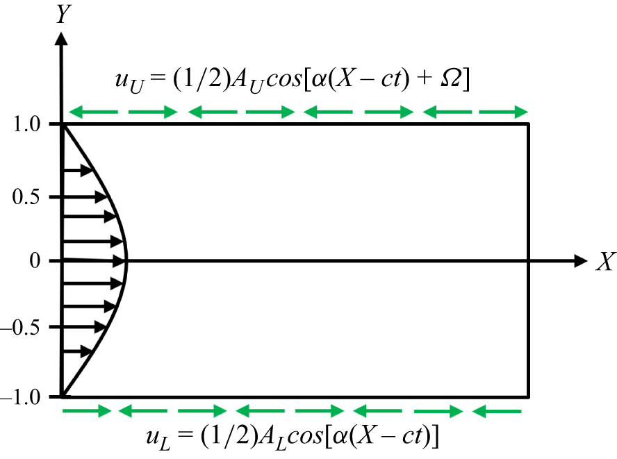
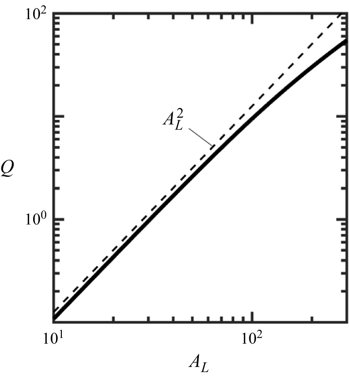


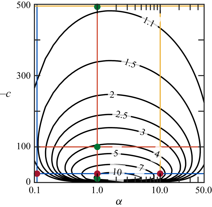


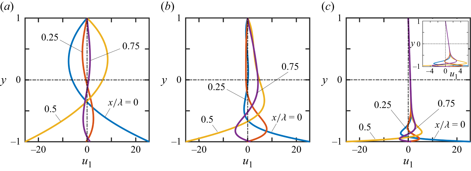


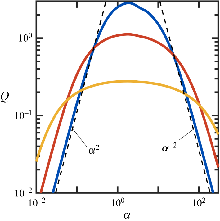


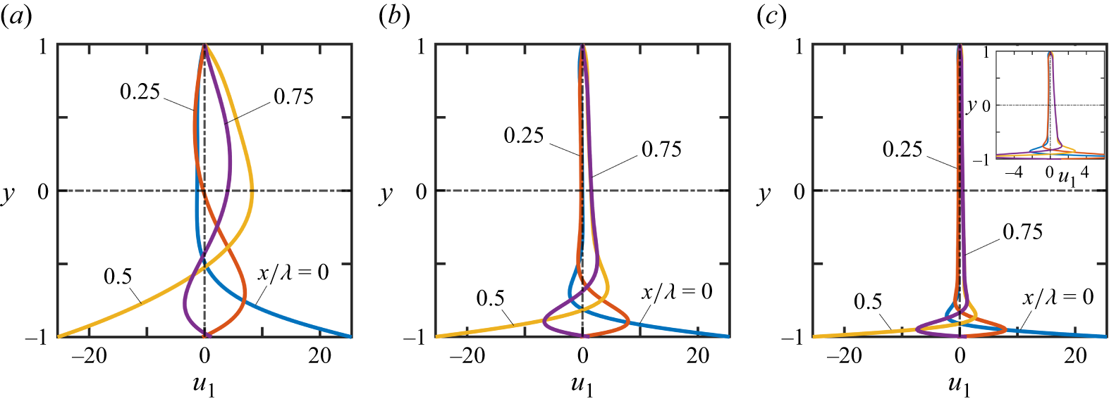


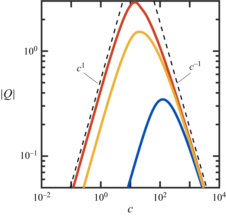


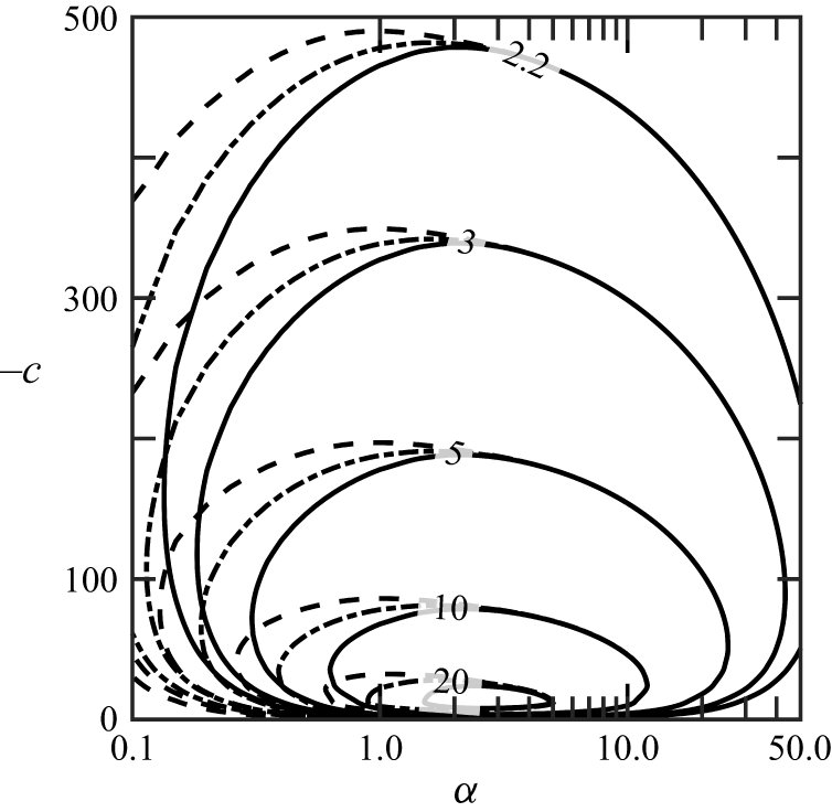


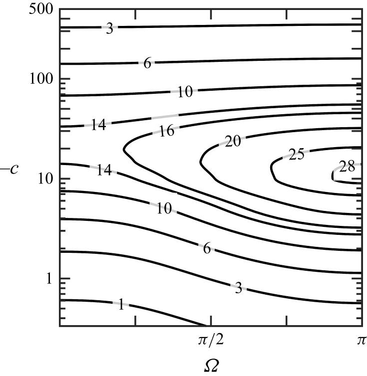


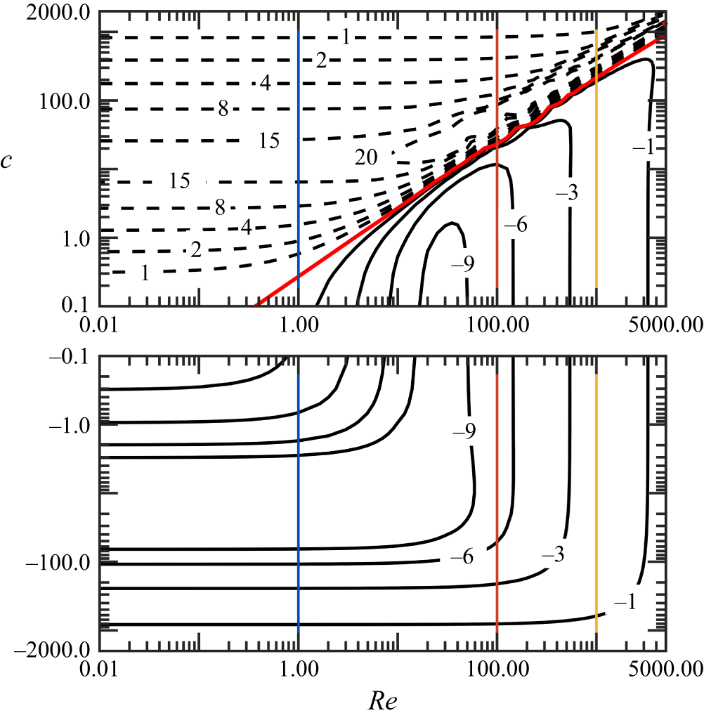


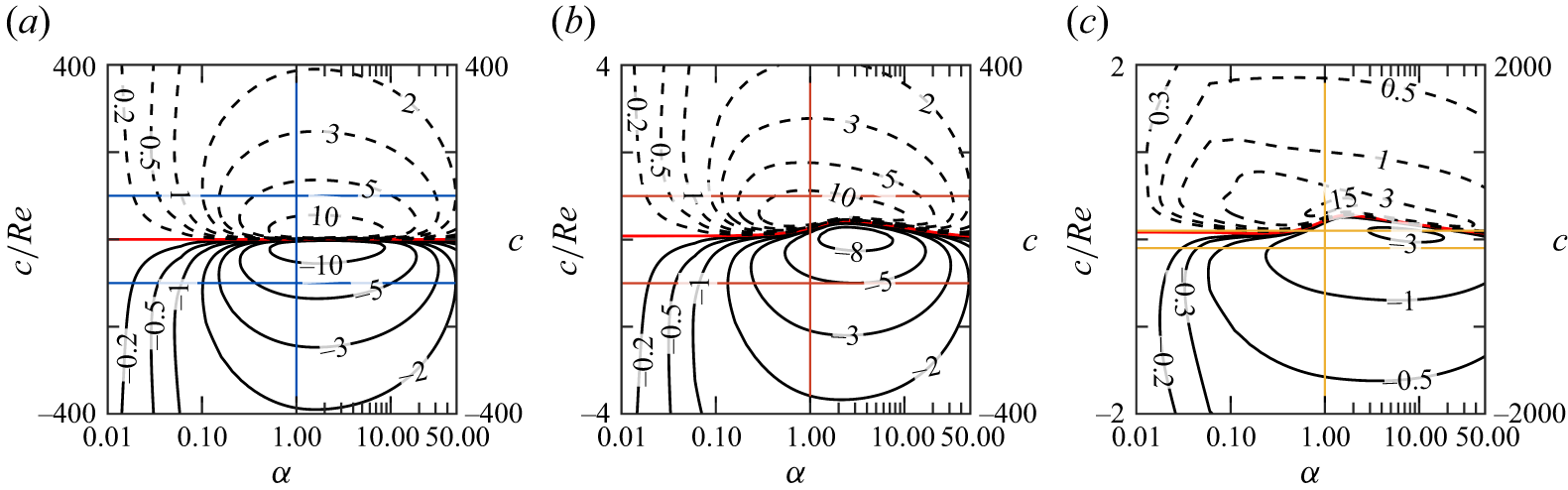


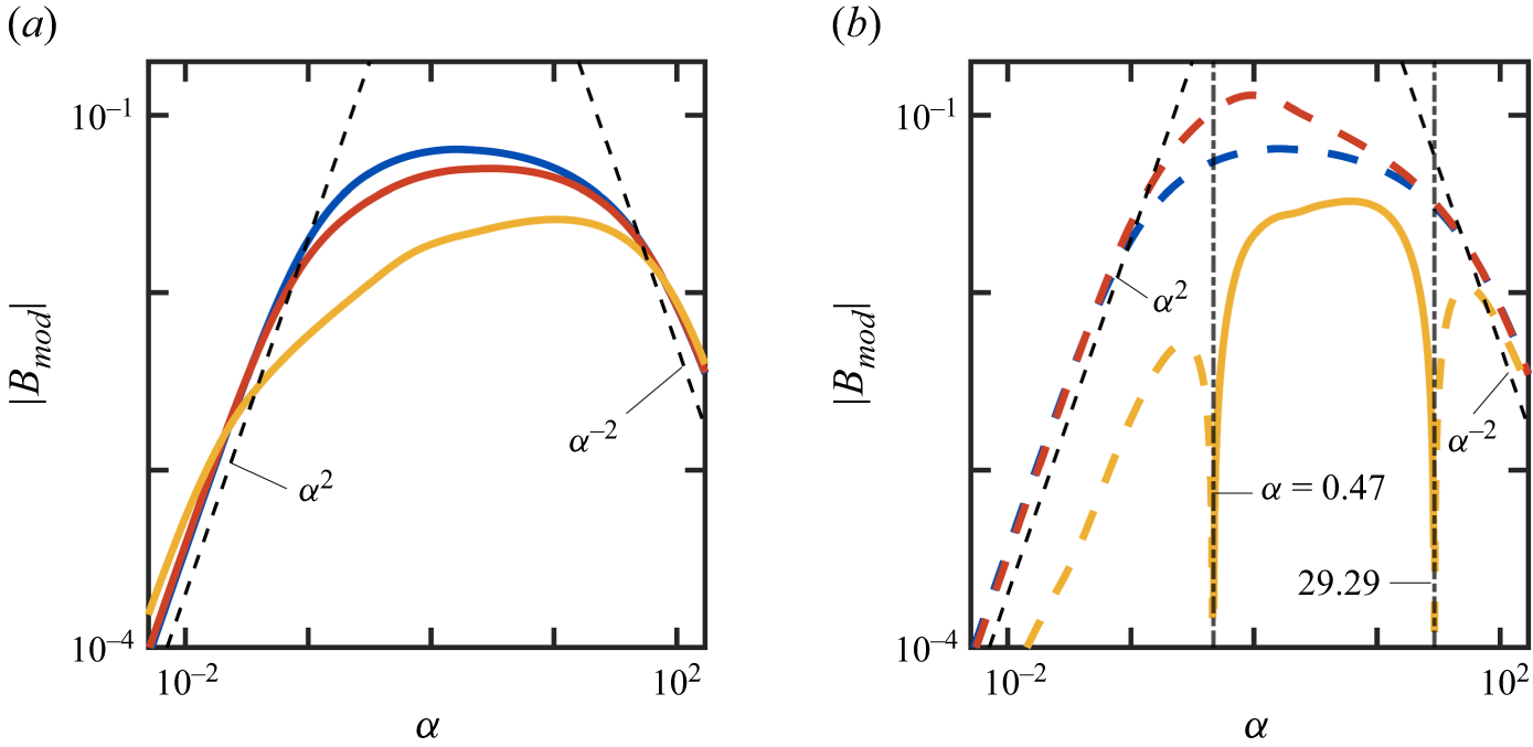


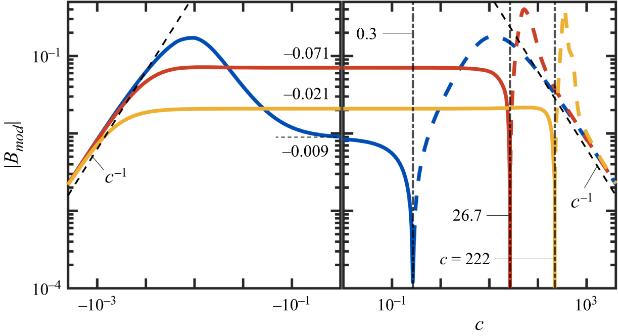


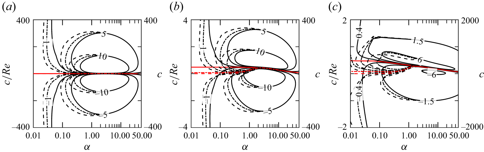


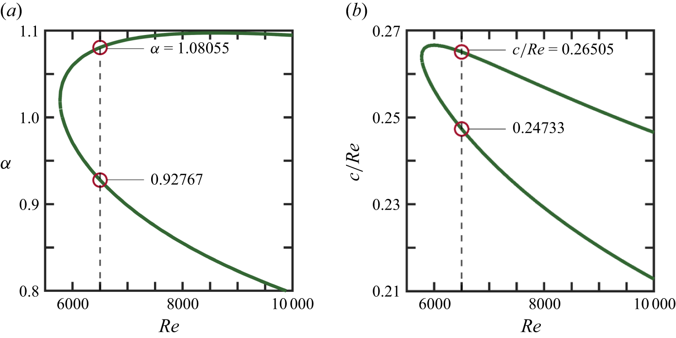


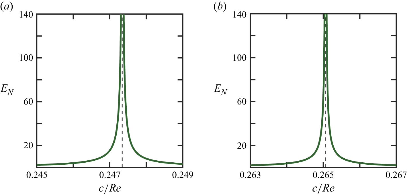


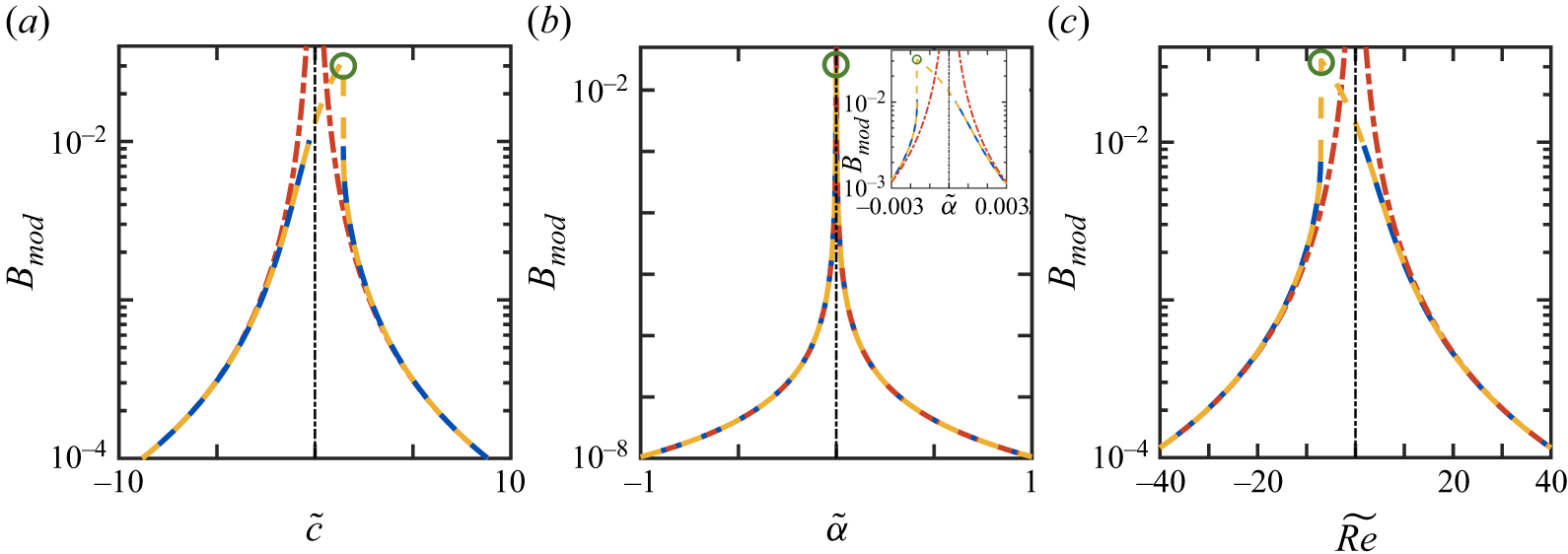


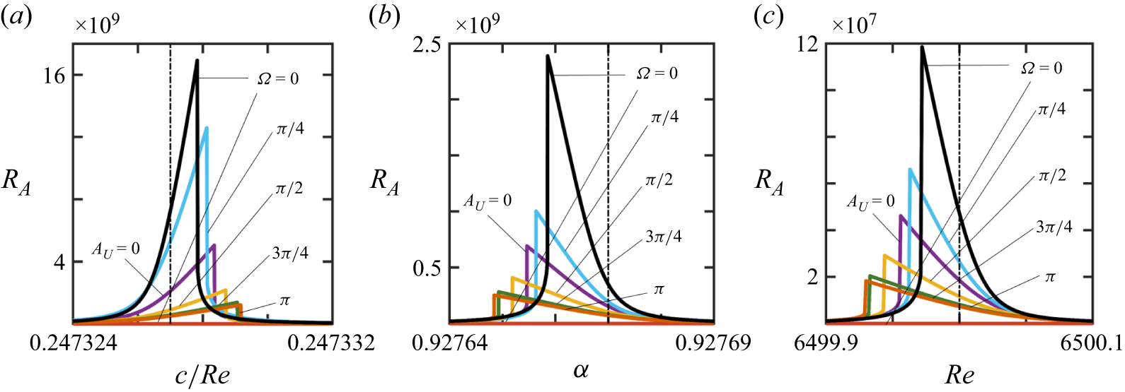


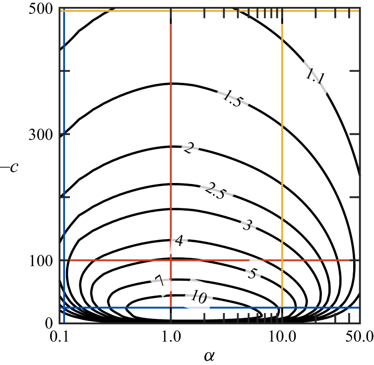


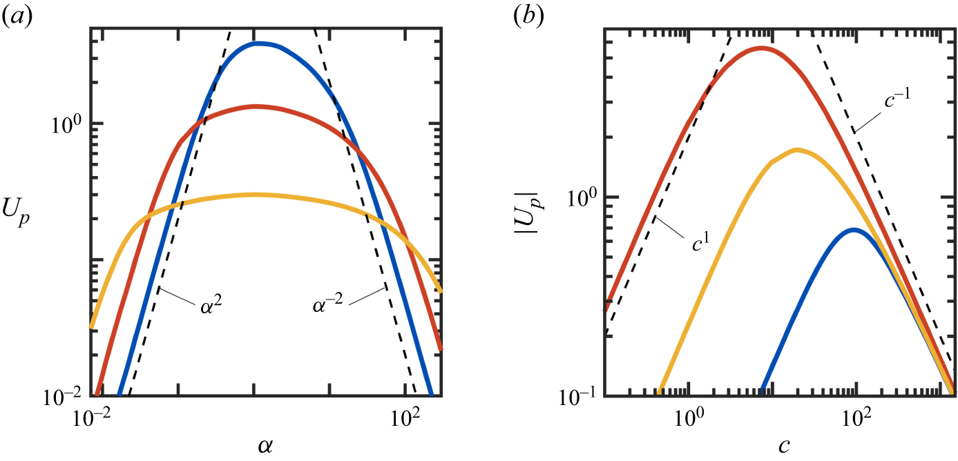


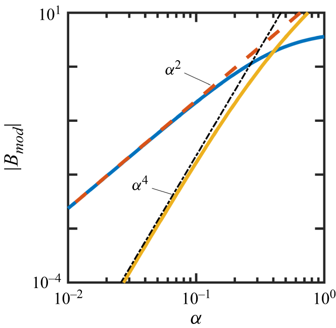


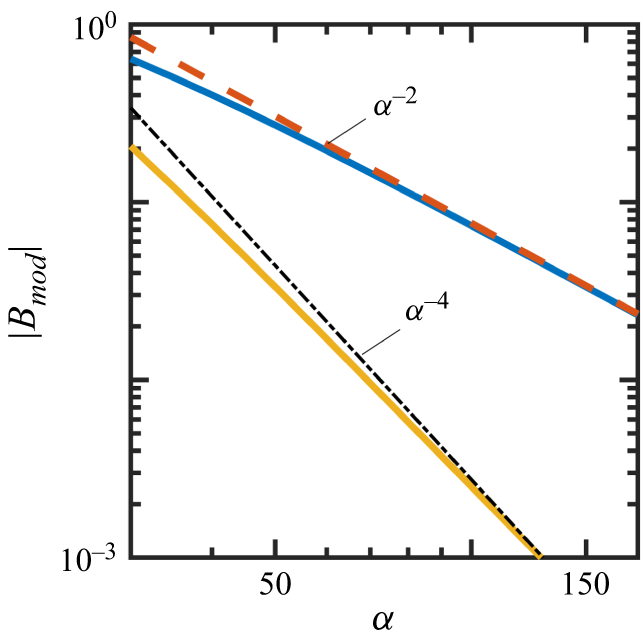


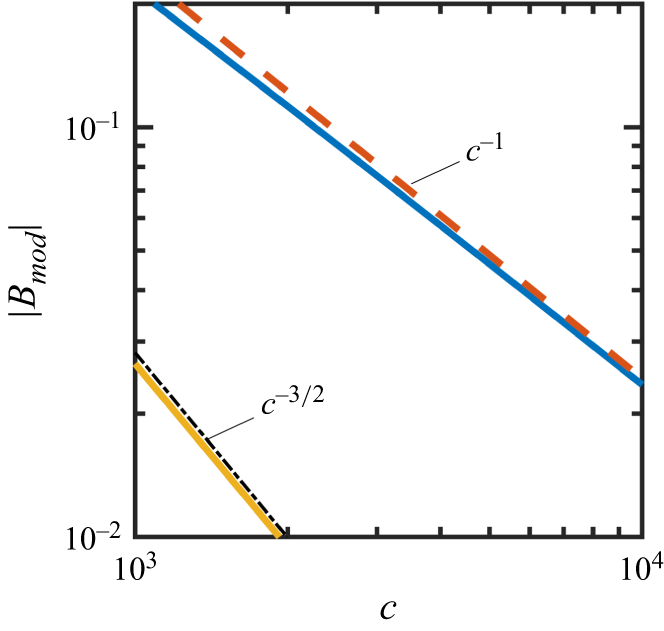


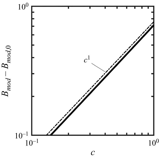


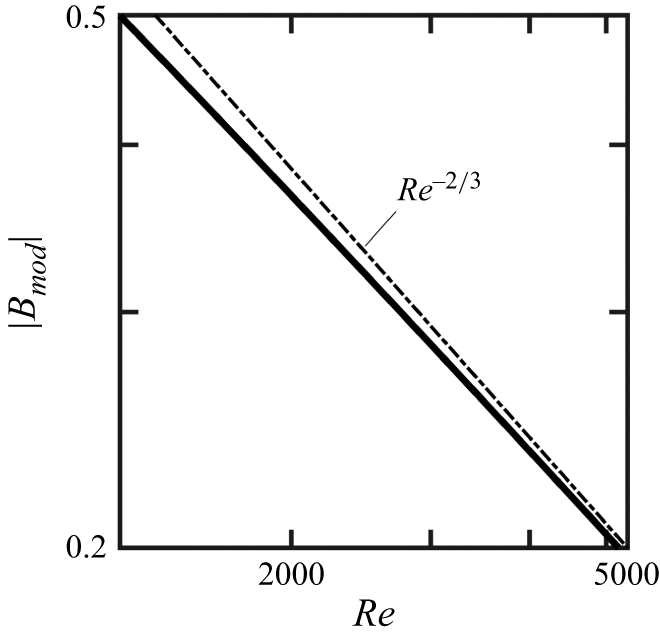


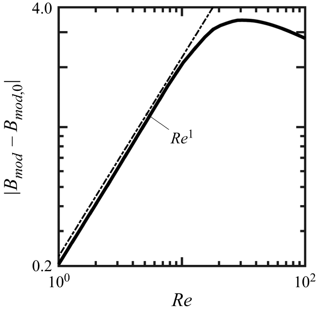


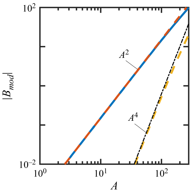


 Open access

