


1. Introduction
Shear-thinning fluids exist in a wide range of industrial processes such as air lubrication (Bobade et al. Reference Bobade, Baudez, Evans and Eshtiaghi2017; Selway, Chan & Stokes Reference Selway, Chan and Stokes2017), aeration (Samaras et al. Reference Samaras, Kostoglou, Karapantsios and Mavros2014), airlift pumps, food processing (McClements Reference McClements2004) and blood pumps (Moyers-Gonzalez, Owens & Fang Reference Moyers-Gonzalez, Owens and Fang2009). Dispersions, such as drops (Ohta et al. Reference Ohta, Iwasaki, Obata and Yoshida2003), bubbles (Premlata et al. Reference Premlata, Tripathi, Karri and Sahu2017) and particles are often found in shear-thinning fluid systems. To control the motion of the dispersion in the sedimentation process (Wang, Wang & Guo Reference Wang, Wang and Guo2006) and the bubble (Iwata et al. Reference Iwata, Yamada, Takashima and Mori2008; Gaudron, Warnez & Johnsen Reference Gaudron, Warnez and Johnsen2015; De Corato et al. Reference De Corato, Saint-Michel, Makrigiorgos, Dimakopoulos, Tsamopoulos and Garbin2019b) or particle (Agi et al. Reference Agi, Junin, Abbas, Gbadamosi and Azli2020) removal process, mechanical vibration and ultrasonic irradiation are often applied. In addition to the utilization of the primary Bjerkness force (Eller Reference Eller1968) that moves the bubble to the node or anti-node for the standing wave, such an oscillatory implementation alters the rheologic property owing to the non-Newtonian nature. As a result, the viscosity is spatially varied, the drag force on the dispersion is reduced and the composite feature of the bubbly or particulate system is modified.
Compared with Newtonian fluids, more complex physical changes may occur during the vibration or oscillation of the shear-thinning fluids. In internal flows, the vibration increases the volumetric flow rate depending on the amplitude and frequency (Barnes, Townsend & Walters Reference Barnes, Townsend and Walters1969, Reference Barnes, Townsend and Walters1971; Deysarkar & Turner Reference Deysarkar and Turner1981; Phan-Thien & Dudek Reference Phan-Thien and Dudek1982a; Siginer Reference Siginer1991; Deshpande & Barigou Reference Deshpande and Barigou2001). Deysarkar & Turner (Reference Deysarkar and Turner1981) also have found flow rate enhancement of a normally stiff paste of fine iron ore and  $16\,\%$ water flowing in a mechanically vibrated tube. When the pulsation of the driving pressure gradient is somewhat weak, the change in the flow rate is proportional to the square of the amplitude (Phan-Thien & Dudek Reference Phan-Thien and Dudek1982a). When the role of viscoelasticity is substantial, the flow enhancement becomes drastic at the resonant frequency (Andrienko, Siginer & Yanovsky Reference Andrienko, Siginer and Yanovsky2000; Casanellas & Ortın Reference Casanellas and Ortın2011; Casanellas & Ortín Reference Casanellas and Ortín2012).
The dynamics of dispersions in resting shear-thinning fluids has been extensively investigated (Acharya, Mashelkar & Ulbrecht Reference Acharya, Mashelkar and Ulbrecht1977; Dekee, Carreau & Mordarski Reference Dekee, Carreau and Mordarski1986), well reviewed by Chhabra (Reference Chhabra2006) and Kulkarni & Joshi (Reference Kulkarni and Joshi2005) and has substantial differences from that in Newtonian fluid. The long-range disturbance caused by the moving sphere (Gu & Tanner Reference Gu and Tanner1985) is reduced due to the shear-thinning effect of the fluid. In flow around a spherical bubble with constant volume rising in a power-law shear-thinning fluid, in which the fluid velocity divided by the bubble radius corresponds to the characteristic shear rate scale and gives the characteristic viscosity, the drag on the bubble is reduced below the corresponding Newtonian value (Dhole, Chhabra & Eswaran Reference Dhole, Chhabra and Eswaran2007a). The local viscosity change greatly depends on the drop shape and is bound to impact the drop rise velocity (Ohta et al. Reference Ohta, Iwasaki, Obata and Yoshida2003, Reference Ohta, Iwasaki, Obata and Yoshida2005). The mass transfer around a bubble (Hirose & Moo-Young Reference Hirose and Moo-Young1969; Michaelides Reference Michaelides2006; Dhole, Chhabra & Eswaran Reference Dhole, Chhabra and Eswaran2007b; Radl, Tryggvason & Khinast Reference Radl, Tryggvason and Khinast2007) or drop (Wellek & Gürkan Reference Wellek and Gürkan1976; Kishore, Chhabra & Eswaran Reference Kishore, Chhabra and Eswaran2007) is increased when the shear-thinning effect is enhanced. Besides, the wall effect induced by a confining tube on the flows around a rigid sphere is seen to be suppressed compared with that in a Newtonian fluid at fixed values of the Reynolds number and diameter ratio (Song, Gupta & Chhabra Reference Song, Gupta and Chhabra2011).
The pulsation, oscillation and acoustic excitation increase the speed of a bubble (Stein & Buggisch Reference Stein and Buggisch2000; Iwata et al. Reference Iwata, Yamada, Takashima and Mori2008; Karapetsas et al. Reference Karapetsas, Photeinos, Dimakopoulos and Tsamopoulos2019), drop (Mendoza-Fuentes et al. Reference Mendoza-Fuentes, Cedeño Madera, Moreno, Zenit, Mena and Manero2018) or particle (Iwamuro, Watamura & Sugiyama Reference Iwamuro, Watamura and Sugiyama2019), and significantly augment the rate of heat transfer in shear-thinning fluids (Gupta, Patel & Chhabra Reference Gupta, Patel and Chhabra2020, Reference Gupta, Patel and Chhabra2021; Mishra, Patel & Chhabra Reference Mishra, Patel and Chhabra2020; Mishra & Chhabra Reference Mishra and Chhabra2021). Qualitatively, the cause is attributed to the reduction in the effective viscosity. Pulsating the power-law shear-thinning fluid with relatively small oscillation amplitude ( $0\leq A \leq 0.8$) over a sphere (Mishra et al. Reference Mishra, Patel and Chhabra2020; Mishra & Chhabra Reference Mishra and Chhabra2021) or a cylinder (Gupta et al. Reference Gupta, Patel and Chhabra2020, Reference Gupta, Patel and Chhabra2021) promotes heat transfer compared with that in non-pulsating flows, which reveals the potential application of the pulsation or oscillation in controlling the heat transfer by varying the kinematic parameters of the flow. For a radially oscillating bubble in the Carreau–Yasuda fluid, De Corato, Dimakopoulos & Tsamopoulos (Reference De Corato, Dimakopoulos and Tsamopoulos2019a) performed numerical simulations under the assumption that the viscosity distribution obeys the spherically symmetric velocity gradient given by potential theory. They showed that the friction coefficient is proportional to ${C_u}^{n-1}$ (here, $C_u$ is the Carreau number and $n$ is the shear-thinning index). In a viscoelastic agarose gel, the ultrasound irradiation changes the effective viscosity in the presence of bubbles, especially at the resonant frequency (Jamburidze et al. Reference Jamburidze, De Corato, Huerre, Pommella and Garbin2017). Although the drag reduction mechanism has been discussed in phenomenologically postulated ways, the detail is not fully clarified owing to the lack of comprehensive analyses.
Our objective is to provide a fundamental perspective on the drag reduction mechanism for oscillatory dispersion in a shear-thinning fluid at a high frequency. For a rigid particle, the oscillatory boundary layer forms near the no-slip wall (Majdalani & Van Moorhem Reference Majdalani and Van Moorhem1997). At a sufficiently high frequency, a remarkably large vorticity is likely to be generated within a very thin boundary layer, making the multiscale system complex. We treat a spherical bubble with a free-slip boundary in the present study. In contrast to the volume change bubble (Iwata et al. Reference Iwata, Yamada, Takashima and Mori2008; De Corato et al. Reference De Corato, Dimakopoulos and Tsamopoulos2019a), the bubble volume remains constant. Neglecting the convective and compressible effects, we consider a creeping incompressible fluid and obtain the solution to the unsteady Stokes equation. Although the assumption of no volume change in the bubble is hypothetical, we choose the simplified system to extract the essence of the drag reduction mechanism. Note that, even for the steady creeping flow, the formulation of the drag force in a shear-thinning fluid (Slattery & Bird Reference Slattery and Bird1961; Hirose & Moo-Young Reference Hirose and Moo-Young1969; Renaud, Mauret & Chhabra Reference Renaud, Mauret and Chhabra2004) must rely on an approximation method because the nonlinearity in the non-Newtonian viscosity expression prevents us from deriving the analytical solution, unlike the case of a Newtonian flow. We perform numerical simulation and modelling for the flow of a well-defined power-law fluid induced by the bubble motion at the prescribed speed. Our research will shed light on the dynamics of bubbles in shear-thinning fluid subjected to ultrasonic irradiation or mechanical vibration.
The rest of this paper is organized as follows. We formulate the problem in § 2.1, comment on some essential parameters in § 2.2 and present some tests to validate the numerical method in § 2.3. In § 3, results are presented and discussed. We investigate the time-averaged velocity and viscosity distribution of the fluid around the bubble to overview the overall features of the fluid flow induced by the oscillatory bubble in § 3.1. In § 3.2, the dependence of the drag force on the power-law index and oscillation amplitude is examined. In § 3.3, we discuss the drag reduction mechanism and provide a theoretical model to predict the time-averaged drag force. In § 4, we provide some vital comments to conclude the paper.
2. Numerical simulation
2.1. General formulation
As shown in figure 1, we consider a spherical bubble with a radius  $a^*$ travelling along the $x^*$ axis direction with a velocity of $U^*$. Hereafter, a superscript $*$ stands for a dimensional quantity. In the present study, the velocity $U^*$ of the bubble consists of two parts: the constant part $U^*_0$, and the oscillatory part $U^*_0A\cos {\omega ^*t^*}$ (here, $A$ is the dimensionless oscillation amplitude, $\omega ^*$ is the angular frequency and $t^*$ is the time) which varies sinusoidally with time. The liquid is regarded as a power-law fluid, for which the viscosity $\mu ^*$ is given by
 \begin{equation} \mu^*=K^*\dot{\gamma^*}^{n-1},\end{equation}
where  $K^*$ is the consistency factor, $\dot {\gamma }^*$ is the shear rate and $n$ is the power-law index, which is limited to $0< n<1$ for the shear-thinning fluid. Note that although the power-law expression (2.1) with the constants $K^*$ and $n$ is usually obtained under steady conditions, it is applied to unsteady flows to facilitate elucidation of the drag reduction mechanism rather than to reproduce the actual phenomena. Upon choosing $a^*$, $U^*_0$, $K^*$ and the density of fluid $\rho ^*$, all the quantities are non-dimensionalized in a way such that
 \begin{equation} \left.\begin{array}{c@{}} U=\dfrac{U^*}{U^*_0}, \quad \omega=\dfrac{\omega^*\rho^*(a^*)^{n+1}}{K^*(U^*_0)^{n-1}},\quad t=\dfrac{t^*K^*(U^*_0)^{n-1}}{\rho^*(a^*)^{n+1}}, \quad \dot{\gamma}=\dfrac{\dot{\gamma}^*a^*}{U^*_0},\\ \boldsymbol{u}=\dfrac{\boldsymbol{u}^*}{U^*_0}, \quad p=\dfrac{p^*(a^*)^n}{K^*(U^*_0)^n},\quad \boldsymbol{\tau}=\dfrac{\boldsymbol{\tau}^*(a^*)^n}{K^*(U^*_0)^n}, \quad \boldsymbol{\mathsf{S}}=\dfrac{\boldsymbol{\mathsf{S}}^*a^*}{U^*_0}, \quad \boldsymbol{\nabla}=a^*\nabla^*, \end{array}\right\} \end{equation}
where  $\boldsymbol {u}$, $p$,
$p$,  $\boldsymbol {\tau }$, $\boldsymbol{\mathsf{S}}$ and $\boldsymbol {\nabla }$ respectively denote the fluid velocity vector, the pressure, the viscous stress tensor, the strain rate tensor and the nabla operator. The non-dimensional velocity of the bubble is
 \begin{equation} U=1+A\cos{\omega t}. \end{equation}
For the incompressible creeping fluid, the equation of continuity and the unsteady Stokes equation are expressed as
 \begin{gather} \boldsymbol{\nabla}\boldsymbol{\cdot}\boldsymbol{u} = 0, \end{gather}
 \begin{gather}\frac{\partial \boldsymbol{u}}{\partial t}={-}\boldsymbol{\nabla} p+\boldsymbol{\nabla}\boldsymbol{\cdot}\boldsymbol{\tau}. \end{gather}
The constitutive equations of the viscosity and the viscous stress tensor are
 \begin{equation} \mu= \dot{\gamma}^{n-1}, \quad \boldsymbol{\tau} =2\mu \boldsymbol{\mathsf{S}}, \end{equation}
where
 \begin{equation} \boldsymbol{\mathsf{S}}=\tfrac{1}{2} ( \boldsymbol{\nabla} \boldsymbol{u}+( \boldsymbol{\nabla} \boldsymbol{u} )^{\rm T} ),\quad \dot{\gamma}=\sqrt{2\boldsymbol{\mathsf{S}}:\boldsymbol{\mathsf{S}}}. \end{equation}
On the bubble wall, we impose the kinematic and free-slip (FS) boundary conditions
 \begin{equation} \boldsymbol{n}\boldsymbol{\cdot}\boldsymbol{u}=\boldsymbol{n}\boldsymbol{\cdot}\boldsymbol{e}_xU, \quad ( \boldsymbol{\tau} \boldsymbol{\cdot} \boldsymbol{n} )\times \boldsymbol{n}={\boldsymbol 0} \text{ at } r=1, \end{equation}
where  $\boldsymbol {n}$ is the unit normal vector pointing outwards on the bubble, and $\boldsymbol {e}_{x}$ is the unit vector in the $x$ direction. At a sufficiently large distance from the bubble, the velocity and the pressure are $\boldsymbol {u}\rightarrow 0$ and $\partial p/\partial r\rightarrow 0$. The force $F$ acting on the oscillatory bubble can be obtained by
 \begin{equation} F ={-}\boldsymbol{e}_x \boldsymbol{\cdot}\oint_{r=1}({-}p\boldsymbol{\mathsf{I}}+\boldsymbol{\tau})\boldsymbol{\cdot}\boldsymbol{n}\, {\rm d}S. \end{equation}
Note that three dimensionless parameters  $n$,
$n$,  $A$ and $\omega$ characterize the behaviour of the system in the present study. Thus, the conversion between the dimensionless and dimensional force (i.e. $F$ and $F^*$) is referred to as
 \begin{equation} F=\frac{F^*(a^*)^{n-2}}{K^*(U^*_0)^n}. \end{equation}
The schematic of the spherical oscillatory bubble travelling in shear-thinning fluid.

2.2. Simulation method
We describe (2.4) and (2.5) in spherical coordinates. The second-order central difference method numerically discretizes the equation set on staggered grids over a two-dimensional domain. For time marching, we apply the second-order Crank–Nicolson method to the viscous term. A simplified-marker-and-cell algorithm (Amsden & Harlow Reference Amsden and Harlow1970) satisfies the momentum equation (2.5) simultaneously with the solenoidal condition (2.4) by means of a direct solution to the pressure equation (Müller & Chan Reference Müller and Chan2019).
We choose the dimensionless angular frequency  $\omega$ and oscillation amplitude $A$ by referring to experimental work using a spherical particle (Iwamuro et al. Reference Iwamuro, Watamura and Sugiyama2019). Considering the liquid density $\rho ^*\sim 10^{3}$ kg $/$m
$/$m $^{3}$, the sound pressure amplitude $({\rm \Delta} p^*)\sim 10^{5}$ Pa, the frequency $f^*\sim 10^{5}$ s $^{-1}$ and the speed of sound $c^*\sim 10^{3}$ m s $^{-1}$, the fluctuating acceleration amplitude is estimated as $({\rm \Delta} \alpha ^*)\sim ({\rm \Delta} p^*)f^*/(\rho ^*c^*) \sim 10^{4}$ m s $^{-2}$. The time-averaged acceleration corresponds to the gravitational acceleration ${\mathcal {G}}\sim 10^1$ m s $^{-2}$. The ratio of the fluctuating force amplitude to the time-averaged drag force would be $({\rm \Delta} \alpha ^*)/{\mathcal {G}}\sim 10^3$, which scales the dimensionless angular frequency $\omega$. The typical fluctuating velocity amplitude in Iwamuro et al. (Reference Iwamuro, Watamura and Sugiyama2019) is estimated as $U_0^* A\sim ({\rm \Delta} p^*)/(\rho ^* c^*)\sim 10^{-1}$ m s $^{-1}$, that is comparable to the fall speed $U_0^*$. Hence, the dimensionless oscillation amplitude $A$ would be of order unity. In the present study, the dimensionless angular frequency is fixed at $\omega =1\times 10^3$, and the amplitude is parametrized in a range of $A\in [0,50]$. The power-law index $n$ is also parametrized in a range of $n\in [0.125,1]$.
We limit the viscosity to  $\mu =\min (\dot {\gamma }^{n-1},\mu _{\max })$, here $\mu _{\max }$ is the maximum viscosity to avoid numerical instability. It is set to $\mu _{\max }=1\times 10^4$, which is confirmed to be large enough for the fluid to be regarded as a purely power-law one. The radius of the computational domain is $1\le r\le R_{\max }$, here, the maximum radius is set to $R_{\max }=1 \times 10^3$. The radial grid width $({\rm \Delta} r)$ increases in geometric progression in the $r$ direction with the minimum $({\rm \Delta} r)_{\min }=1 \times 10^{-2}$. The number of grid points is $N_r\times N_\theta =128 \times 128$ in the $r$ and $\theta$ directions. The time increment is fixed at ${\rm \Delta} t=2{\rm \pi} /(2^{10} \omega )$, which is confirmed to be small enough to capture the unsteady behaviours. Following Sugiyama & Takemura (Reference Sugiyama and Takemura2010), we employ a numerical method that uses the exact values of the grid width, the cell interfacial area and the control volume in spherical coordinates, and also guarantees the conservation law in a discretized equation. We performed convergence tests of the total energy dissipation rate $\dot {E}_{diss}$, which is determined from the numerical integral of $\dot {\gamma }^{n+1}$ over the entire computational domain. We confirmed the grid convergence behaviours with decreasing $({\rm \Delta} r)_{\min }$ and with increasing $N_r(=N_\theta )$. We also confirmed the energy balance relation that the time-averaged $\dot {E}_{diss}$ is in good agreement with the time-averaged energy input corresponding to $FU$, where $F$ is numerically evaluated on the bubble wall. Further, we verified the Bobyleff–Forsythe formula (which will be discussed in § 3.3), involving the surface integral of the enstrophy and the volume integrals of the enstrophy and the strain rate square, holds exactly. The accuracy assessment indicates that the simulated results using the present computational mesh are accurate enough for the subsequent discussion of surface and bulk quantities.
2.3. Validation tests
Validation simulations of fluid flow induced by a sphere travelling in a shear-thinning fluid with no oscillation ( $U=1$) have been conducted. Firstly, we check the validity for a no-slip (NS) sphere since there are several available data in the literature. For the NS sphere, the boundary condition (2.8a,b) is replaced by ${\boldsymbol u}=\boldsymbol {e}_x U$. Figure 2 shows the relation between the drag force $F$ and the power-law index $n$. In figure 2(a) for the NS sphere, the circle symbols and the solid curve respectively indicate the present numerical results and an empirical expression (Renaud et al. Reference Renaud, Mauret and Chhabra2004), corresponding to
 \begin{equation} F = 4{\rm \pi} \left(\frac{3\sqrt{6}}{2(n^2+n+1)} \right)^{n+1}. \end{equation}
Note that (2.11) was formulated in such a way as to take the analytical value  $6{\rm \pi}$ for the Newtonian case ( $n=1$) and to comprehensively capture the variation for any shear-thinning power-law fluid ( $0< n<1$). The present results are in good agreement with the empirical curve (2.11) over the entire range of $n$. However, a slight discrepancy is found upon more careful inspection. The cause would be the imperfect accuracy of the empirical expression (2.11). The cross symbols in figure 2(a) indicate the well-validated data of direct numerical simulations (Missirlis et al. Reference Missirlis, Assimacopoulos, Mitsoulis and Chhabra2001). These are supposed to be more accurate than (2.11). The present results are in exact agreement with the data from the simulation (Missirlis et al. Reference Missirlis, Assimacopoulos, Mitsoulis and Chhabra2001), and we can assert that the discrepancy between the present numerical results and the result predicted by (2.11) is attributed to the underestimation of (2.11). Thus, the present numerical method can reasonably treat the shear-thinning power-law viscosity and solve the equations of the steady creeping flow around the NS sphere.
The force  $F$ vs the power-law index $n$ for steady creeping flow. The circle symbols indicate the present numerical results. (a) For the NS sphere, the solid curves and the cross symbols indicate the empirical expression (2.11) and the numerical results of Missirlis et al. (Reference Missirlis, Assimacopoulos, Mitsoulis and Chhabra2001), respectively. (b) For the spherical bubble, the solid and dashed curves indicate the semi-analytical expressions (2.12) and (A14) for $0<1-n\ll 1$.

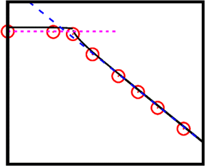
Secondly, let us determine the spherical bubble's validation in a steady creeping flow. Since such studies are significantly fewer than those of the NS sphere, accessible reference data are limited in the literature. In figure 2(b) for the spherical bubble, the circle symbols and the solid curve respectively indicate the present results and a semi-analytical expression (Hirose & Moo-Young Reference Hirose and Moo-Young1969), corresponding to
 \begin{equation} F =\frac{4 {\rm \pi}\ 3^{(n-1)/2}(13+4n-8n^2)}{(2n+1)(n+2)}, \end{equation}
which was derived under the assumption that the deviation from Newtonian flow is small (namely the power-law index  $n$ is close to unity (i.e. $0< 1-n \ll 1$)), and gives exact value $4{\rm \pi}$ for the Newtonian fluid case $n=1$. Reconsidering this assumption, we also derive another expression (A14) in a straightforward way (see Appendix A). It is drawn in the dashed curve in figure 2(b). For $n\approx 1$ where the precondition in the analyses (Hirose & Moo-Young Reference Hirose and Moo-Young1969) and Appendix A is fulfilled, the present results are in good agreement with the curves (2.12) and (A14). Thus, the present numerical method can reasonably treat the power-law viscosity and the FS condition in steady creeping flows. Note that, although the validity of both the expressions (2.12) and (A14) may be violated for small $n$, figure 2(b) exhibits the consistency between the present semi-analytical expression (A14) and numerical results for $n\approx 1$, and also the incidental consistency over a wider range of $n$.
$n$.
We have also assessed the present numerical method to predict flows induced by an oscillating spherical bubble in a Newtonian fluid (with the index of  $n=1$). For the bubble velocity $U=\cos {\omega t}$, the angular frequency was parametrized in a range of $10^{-1}\le \omega \le 10^3$. For all the conditions of $\omega$, the numerical results of the temporal change in the force $F$ were confirmed to be in excellent agreement with the analytical solution (Yang & Leal Reference Yang and Leal1991)
 \begin{equation} F={Re}\left\{\left(\frac{2{\rm \pi}}{3}{\rm i}\omega+\frac{4{\rm \pi}\left(1+({\rm i}\omega)^{1/2} \right)}{1+\frac{1}{3}({\rm i}\omega)^{1/2}}\right) \exp({\rm i}\omega t)\right\}. \end{equation}
The respective effects of the shear-thinning fluid and the oscillation have been validated. The results of numerical simulations by combining these effects will be presented in § 3.
3. Simulation results
3.1. Velocity and viscosity distribution around the bubble
To overview how the fluid flow is induced owing to the interplay between  $n$ and $A$, the time-averaged velocity and viscosity distribution are investigated. In consideration of the facts that the system is axisymmetric and the radial velocity component $u_r$ is expanded in a Legendre polynomial series, we focus on the radial profile of the first mode $\langle \hat {u}_r\rangle$:
 \begin{equation} \langle\hat{u}_r\rangle(r) =\frac{3}{2}\left\langle\int_{0}^{\rm \pi} u_r(r,\theta,t)\cos{\theta}\sin{\theta}\, \mathrm{d}\theta \right\rangle, \end{equation}
where  $\langle \cdots \rangle (=\omega (2{\rm \pi} )^{-1}\int _{0}^{2{\rm \pi} / \omega } \cdots \mathrm {d}t)$ stands for the time average over one cycle. Figure 3 shows the simulated results of $\langle \hat {u}_r\rangle$ as a function of $r$. For comparison, two analytical curves ( $\langle \hat {u}_r\rangle =r^{-3}$ for the potential flow and $\langle \hat {u}_r\rangle =r^{-1}$ for the Newtonian Stokes flow) with no oscillation $A=0$ are included therein.
The relation of the time-averaged velocity coefficient  $\langle \hat {u}_r\rangle$ as a function of $r$ in the fully developed state for various power-law indices $n$ and oscillation amplitudes $A$. The solid and dashed curves indicate $\langle \hat {u}_r\rangle =r^{-3}$ for the potential flow and $\langle \hat {u}_r\rangle =r^{-1}$ for the steady Newtonian Stokes flow, respectively. The symbols correspond to the simulated results, where the $r$ positions for the conditions ( $A=0$, $0.1$, $1$,
$1$,  $10$) specified by the symbol types are separated to make the respective profiles comprehensible. The inset shows the log–log plot to clarify the curve slope; (a) $n=0.125$, (b) $n=0.25$, (c) $n=0.75$ and (d) $n=1$.

For  $n=1$ (figure 3d), corresponding to the Newtonian fluid, the plots of $\langle \hat {u}_r\rangle$ collapse onto the monopole curve $r^{-1}$ irrespective of the oscillation amplitude $A$. This is a natural consequence of the system linearity involved in the Newtonian Stokes equation. The time-average process offsets the oscillation effect. For $0< n<1$ (figure 3a–c), corresponding to the shear-thinning fluid, the slope of the profile $\langle \hat {u}_r\rangle$ is steeper with decreasing power-law index $n$. The viscosity distribution, depending upon the spatial variation of the shear rate, is reflected in such an $n$-dependent decaying behaviour. For $A=0$, the slope at $n=0.75$ (figure 3c) is between $-1$ (the Newtonian Stokes flow) and $-3$ (the potential flow), while the profiles at the sufficiently small indices $n=0.125$ (figure 3a) and $n=0.25$ (figure 3b) decay more rapidly than the potential flow one. For each $n$ condition, the profiles with varying $A$ are non-monotonic because the nonlinear viscosity to the shear rate is affected by the oscillation amplitude $A$. Therefore, the bubble oscillation alters the time-averaged viscosity and stress distributions. Carefully observing figure 3(a–c), one finds that, with increasing $A$, the profile becomes closer to that of the potential flow, implying that the time-averaged vorticity is attenuated in the bulk. At each instant, the vorticity generated on the bubble surface ( $r=1$) is $2\{u_\theta +(1+A\cos \omega t)\sin \theta \}$ due to the FS condition (Ryskin & Leal Reference Ryskin and Leal1984), and thus its magnitude is likely to be larger with increasing $A$. However, it is evident from figure 3(a–c) that the large amplitude oscillation (with the large $A$) of the bubble in the strong shear-thinning fluid (with the small power-law index $n$) confines the enhanced vorticity to near the bubble wall and hinders the vorticity transfer to the bulk.
For steady flows, the interplay between the spatially non-uniform viscosity and the motion of dispersion (i.e. a bubble, drop or particle) has been investigated by several researchers (e.g. Ohta et al. Reference Ohta, Iwasaki, Obata and Yoshida2005; Zhang, Yang & Mao Reference Zhang, Yang and Mao2010; Zare, Daneshi & Frigaard Reference Zare, Daneshi and Frigaard2021). Following the earlier studies, to demonstrate the effect of the oscillation amplitude  $A$ on the shear-thinning viscosity, figure 4 visualizes the distribution of the time-averaged viscosity $\langle \mu \rangle$ around the bubble at $n=0.25$. The colour map exhibits that, for $A \lesssim 1$, the low viscosity region becomes smaller with increasing $A$, while it becomes larger for $A \gtrsim 1$. A simple rough relation may account for a non-monotonic volume change in the low viscosity region. Under the assumption that the shear rate scales linearly to the bubble velocity magnitude $|U|$, namely $\dot {\gamma }\sim |1+A\cos \omega t|/\ell$ (here, the length scale $\ell$ is hypothetically fixed), the instantaneous viscosity scales as $\mu \sim |1+A\cos \omega t|^{n-1}$. With this relation, for a sufficiently small amplitude $0< A\ll 1$, the time-averaged viscosity may scale as $\langle \mu \rangle \sim 1+(1-n )(2-n )A^2/4$, which increases with $A$ as long as $0< n<1$, while for the sufficiently large amplitude $A\gg 1$, it may scale as $\langle \mu \rangle \sim A^{n-1}$, which decreases with $A$. Therefore, $\langle \mu \rangle$ is inferred to be maximized at a moderate $A$. The high viscosity region (corresponding to the non-coloured area in figure 4) is the largest at the moderate amplitude $A=1$. Note that, even though the non-monotonic behaviour of the shear-thinning viscosity with varying $A$ is explainable in terms of the bubble velocity, unlike a steady flow, the time-averaged viscosity $\langle \mu \rangle$ in the unsteady flow is not necessarily correlated with the time-averaged force $\langle F\rangle$. It is because the time-averaged viscous stress, which is given by $\langle {\boldsymbol \tau }\rangle =\langle 2\mu \boldsymbol{\mathsf{S}}\rangle \neq 2\langle \mu \rangle \langle \boldsymbol{\mathsf{S}}\rangle$, is not proportional to $\langle \mu \rangle$. To discuss the time-averaged force on the bubble in a strong shear-thinning fluid, we will consider a nearly irrotational velocity field with a large amplitude oscillation (figure 3a,b). Further, we will examine the overall energy balance in the unsteady fluid motion rather than the viscosity distribution.
The time-averaged viscosity distribution around the bubble in a fully developed state for various amplitudes  $A$ at the power-law index of $n=0.25$; (a) $A=0$, (b) $A=0.1$, (c) $A=1$ and (d) $A=10$.

3.2. The effect of the oscillation amplitude  $A$ on the force acting on the bubble

Figure 5 shows the temporal change in the force  $F$ at the power-law index of $n=0.25$ and its velocity $U(=1+A\cos \omega t)$ for various oscillation amplitudes $A$. Here, we shall separately discuss the fluctuating and time-averaged components of $F$. Firstly, on the fluctuating force, we confirm that the amplitude of $F$ is approximated by $2{\rm \pi} \omega A/3$ and the phase difference between $F$ and $U$ is approximately ${\rm \pi} /2$. These features imply that the fluctuating component of $F$ is consistent with the added inertia force $-(2{\rm \pi} \omega A/3)\sin \omega t$ on a translationally oscillating sphere, indicating that the potential flow well describes the fluctuating velocity distribution at each instant. In Newtonian fluid flows, as indicated in (2.13) with a conversion of $\omega \Rightarrow \omega A$, such a potential approximation is valid for sufficiently high frequency $\omega \gg 1$. This is because the amplitude of the added inertia force (corresponding to the first term inside the curly brackets in (2.13)) is proportional to $\omega A$ and is much greater than that of the history force (corresponding to the second term), likely to be proportional to $(\omega A)^\beta$ with $\beta \le 1/2$. This relation of the added inertia force would also hold for the non-Newtonian power-law fluid flow at $\omega =1\times 10^3\gg 1$ in the present study. Since the added inertia force is expressed as a temporally sinusoidal function proportional to $\sin \omega t$, it makes no contribution to the time-averaged component.
Temporal change in the force  $F$ on the bubble (solid curve) and its velocity $U(=1+A\cos \omega t)$ (dashed curve) for one cycle in the fully developed state for various oscillation amplitudes $A$ at the power-law index of $n=0.25$. The horizontal axis is in scaled time $t/T$, and here $T(=2{\rm \pi} /\omega )$ is the period; (a) $A=0.01$, (b) $A=0.1$, (c) $A=1$ and (d) $A=10$.

Secondly, we pay attention to the time-averaged drag force denoted by  $D(=\langle F\rangle )$. Figure 6(a) shows the relation between $D$ and $A$. When the amplitude $A$ is sufficiently smaller than unity, the drag force $D$ approaches that with no oscillation $D_0$. For $A \gtrsim 1$, $D$ substantially decreases with increasing $A$. This result implies that the shear-thinning effect, enhanced with $A$, causes the drag reduction. This is unlike the fluctuating component of the force $F$, for which the amplitude increases with $A$ (figure 5) owing to the added inertia force. To highlight the deviation of the time-averaged drag force with oscillation $D$ from that with no oscillation $D_0$, figure 6(b) depicts the drag reduction ratio $(DRR(=1-D/D_0))$ as a function of the oscillation amplitude $A$. For $A\lesssim 1$, $DRR$ is likely to be proportional to $A^2$, while for $A\gtrsim 1$, $DDR$ is saturated to $1$ (corresponding to the upper bound as long as $D>0$) with increasing $A$. The proportionality of $DDR \propto A^2$ rather than $A^1$ for sufficiently small $A$ comes from the nonlinearity in the power-law viscosity and is explained from the idea of the weakly nonlinear perturbation method. Assuming $0< A\ll 1$, which is chosen as a perturbation, we write the time-dependent force in a series form as $F=D_0+\alpha _1 A^1+\alpha _2 A^2+\cdots$ for each $n$ (here, $\alpha _1=\alpha _1(t)$ and $\alpha _2=\alpha _2(t)$ are time-dependent functions). In the present system, the $O(A^1)$ contribution has the time dependence on $\cos {\omega t}$ and/or $\sin {\omega t}$. Hence, the time-averaged value thereof vanishes (i.e. $\langle \alpha _1\rangle =0$). In contrast, the $O(A^2)$ contribution comes from the correlation between the $O(A^1)$ variations in the viscosity and the strain rate. It involves the time dependence of $\cos ^2\omega t$ and/or $\sin ^2\omega t$. Hence, the time-averaged value thereof is non-zero (i.e. $\langle \alpha _2\rangle \neq 0$), and the second-order approximation of the time-averaged drag force is expressed as $D=D_0+\langle \alpha _2\rangle A^2$, accounting for the relation of $1-D/D_0 \propto A^2$, as seen for $A\lesssim 1$ in figure 6(b). Note that Phan-Thien & Dudek (Reference Phan-Thien and Dudek1982b) demonstrated a similar mechanism of the second-order drag reduction in pulsating pipe flows of a polymeric fluid owing to the viscosity's nonlinearity.
The relationship between time-averaged drag force  $D$ and oscillation amplitude $A$ at the power-law index of $n=0.25$. The circle symbols indicate the simulated results. Here, $D_0(=30.32)$ is the drag force with no oscillation( $A=0$). Panel (a) shows $D$ vs $A$. The solid curve represents $D_0$. Panel (b) shows a log–log plot of the drag reduction ratio $(DRR(=1-D/D_0))$ vs $A$. The solid line corresponds to a curve with a slope of $2$, namely $DRR \propto A^2$.

For sufficiently large  $A$, the saturation of $1-D/D_0 \approx 1$ in figure 6(b) indicates that the time-averaged drag force becomes small enough ( $D\ll D_0$). To highlight how such an intense drag reduction depends upon the power-law index $n$, figure 7 depicts the drag reduction behaviour for various $n$: the log–log plot of the time-averaged scaled drag force $D/D_0$ vs $A$ (figure 7a) and the slope $d (\log D)/ d (\log A)$ vs $A$ (figure 7b). In figure 7(a), the simulated results for $A\gtrsim 1$ exhibit a constant slope in the decaying profile for each $n$. The solid lines indicate the fitted curves proportional to $A^{n-1}$, which capture the simulated results for the respective $n$ as long as the amplitude $A$ is large enough. Figure 7(b) corresponds to the slopes of the curves in figure 7(a), indicating the shear-thinning effect for each $n$. The fluid with a smaller power-law index $n$ has the stronger shear-thinning effect and the scaled drag force on the bubble in it is more significantly reduced, corresponding to the same amplitude of oscillation. Note that a similar power law in the drag reduction was found for a radially oscillating bubble rising in a shear-thinning fluid (De Corato et al. Reference De Corato, Dimakopoulos and Tsamopoulos2019a). De Corato et al. (Reference De Corato, Dimakopoulos and Tsamopoulos2019a) could separately treat the radial and translational motions of the bubble with two velocity scales $\dot {R}$ and $U$. The viscosity distribution affected by $\dot {R}$ was assumed to be spherically symmetric. In contrast, we cannot separately treat the effect of the constant and oscillatory velocities of the bubble. Thus, in the present study, the shear-thinning viscosity is affected by both motions, and its distribution is not spherically symmetric. Subsequently, we will discuss the drag reduction mechanism resulting in the expression of $D/D_0 \propto A^{n-1}$.
The relation between the time-averaged scaled drag force  $D/D_0$ and the oscillation amplitude $A$ for various power-law indices $n$. The symbols represent the simulated results with the respective power-law index $n$ specified in the panel. Panel (a) shows $D/D_0$ vs $A$. The solid curve for each $n$ indicates the curve proportional to $A^{n-1}$. Panel (b) shows $d (\log D)/ d (\log A)$ vs $A$, corresponding to the slope in (a). The solid curve for each $n$ indicates the value of $n-1$.

3.3. Discussion of the drag reduction mechanism
We now investigate how the vorticity is generated on the bubble wall, is distributed over the space and affects the force due to the interplay between the FS boundary condition and the high frequency. Before examining the non-Newtonian fluid flow, we shall recall the Newtonian one, including a sphere with a velocity of  $U=1+A\cos \omega t$. On a NS sphere, the force $F_{{NS}}$ is written in a form (Landau & Lifschitz Reference Landau and Lifschitz1987)
 \begin{equation} F_{{NS}}=6{\rm \pi}+{Re}\left\{ A\left(\frac{2{\rm \pi}}{3}{\rm i}\omega+6{\rm \pi} ({\rm i}\omega )^{1/2}+6{\rm \pi}\right)\exp({\rm i}\omega t)\right\}, \end{equation}
where the first and second terms on the right-hand side are the steady drag force associated with the constant unity velocity and the force with oscillatory velocity  $A\cos \omega t$, respectively. In (3.2), the first, second and third terms inside the parentheses before $\exp (\textrm {i}\omega t)$ indicate the added inertia force, the Basset history force and the drag force, respectively. On a spherical bubble (referred to as a FS sphere), the general expression of the force $F_{{FS}}$ for arbitrary angular frequencies $\omega$ is given by the combination of $4{\rm \pi}$ (associated with the constant unity velocity) and (2.13) multiplied by the amplitude $A$ (associated with $A\cos \omega t$). At sufficiently high frequencies ( $\omega \gg 1$), $F_{{FS}}$ is simplified into
 \begin{equation} F_{{FS}}=4{\rm \pi}+{Re}\left\{A\left(\frac{2{\rm \pi}}{3}{\rm i}\omega+12{\rm \pi}+O(\omega^{{-}1/2})\right)\exp({\rm i}\omega t)\right\}. \end{equation}
In (3.3), the first and second terms inside the parentheses before  $\exp (\textrm {i}\omega t)$ indicate the added inertia and Levich drag forces, respectively (Magnaudet & Eames Reference Magnaudet and Eames2000; Liu, Sugiyama & Takagi Reference Liu, Sugiyama and Takagi2016). The term of order $\omega ^{-1/2}$ vanishes when $\omega \gg 1$. Here, we pay attention to the temporally oscillatory force, i.e. the second term in (3.2) and (3.3). At high frequencies, for the NS sphere, the penetration depth $\ell$ of the rotational flow is of the order $\omega ^{-1/2}$ (Landau & Lifschitz Reference Landau and Lifschitz1987), and hence the magnitude of the vorticity generated on the sphere wall scales as $\ell ^{-1}\sim \omega ^{1/2}$. By contrast, for the bubble, the vorticity magnitude scales as $\omega ^0$ owing to the FS condition (Ryskin & Leal Reference Ryskin and Leal1984). The difference in the order of the generated vorticity magnitude is reflected in the presence (3.2) or absence (3.3) of the $O(\omega ^{1/2})$ term in the force expression. Note that, for the bubble, the temporally oscillatory force (corresponding to the second term in (3.3)) is consistent with the force in a viscous potential flow (Joseph Reference Joseph2006), which is irrotational but involves the viscous dissipation mechanism, even though it is derived in the low Reynolds number limit. Such a consistent expression is justified as long as the vorticity magnitude in the bulk is negligible. Although this feature is reflected in the force expression (3.3) for the Newtonian creeping flow, the mechanism of the negligible bulk vorticity would be explained by that the interplay between the FS condition and the high frequency hinders the vorticity diffusion irrespective of Newtonian or non-Newtonian fluid.
Again, we will see the simulation results. Quantifying the level of bulk vorticity, we will discuss the applicability of the potential flow theory to the non-Newtonian power-law fluid. To this end, we employ the Bobyleff–Forsythe (BF) formula (Serrin Reference Serrin1959; Kang & Leal Reference Kang and Leal1988; Stone Reference Stone1993) for any velocity field  ${\boldsymbol v}$ satisfying the solenoidal condition $(\boldsymbol {\nabla }\boldsymbol {\cdot }{\boldsymbol v}=0)$ and the kinematic and FS boundary conditions (2.8a,b), which are expressed as
 \begin{equation} \beta_1(\boldsymbol v)=\beta_2(\boldsymbol v)+\beta_3(\boldsymbol v), \end{equation}
where
 \begin{equation}
\left.\begin{array}{c@{}} \displaystyle \beta_1(\boldsymbol
v)=\tfrac{1}{2}\int_V (\boldsymbol{\nabla}{\boldsymbol
v}+(\boldsymbol{\nabla}{\boldsymbol v})^{\rm
T}):(\boldsymbol{\nabla}{\boldsymbol
v}+(\boldsymbol{\nabla}{\boldsymbol v})^{\rm T})\, {\rm
d}V,\\ \displaystyle \beta_2(\boldsymbol v)=\int_V
{\boldsymbol \varpi}\boldsymbol{\cdot}{\boldsymbol
\varpi}\, {\rm d}V,\quad \beta_3(\boldsymbol
v)=\tfrac{1}{2}\oint_{r=1}{\boldsymbol
\varpi}\boldsymbol{\cdot}{\boldsymbol \varpi}\, {\rm d}S,
\end{array}\right\} \end{equation}
\begin{equation}
\left.\begin{array}{c@{}} \displaystyle \beta_1(\boldsymbol
v)=\tfrac{1}{2}\int_V (\boldsymbol{\nabla}{\boldsymbol
v}+(\boldsymbol{\nabla}{\boldsymbol v})^{\rm
T}):(\boldsymbol{\nabla}{\boldsymbol
v}+(\boldsymbol{\nabla}{\boldsymbol v})^{\rm T})\, {\rm
d}V,\\ \displaystyle \beta_2(\boldsymbol v)=\int_V
{\boldsymbol \varpi}\boldsymbol{\cdot}{\boldsymbol
\varpi}\, {\rm d}V,\quad \beta_3(\boldsymbol
v)=\tfrac{1}{2}\oint_{r=1}{\boldsymbol
\varpi}\boldsymbol{\cdot}{\boldsymbol \varpi}\, {\rm d}S,
\end{array}\right\} \end{equation}
and  ${\boldsymbol \varpi }=\boldsymbol {\nabla }\times {\boldsymbol v}$ is the vorticity. Note that $\beta _k\ge 0$ for $k=1$, $2$ and $3$. The BF formula (3.4) characterizes the contributions of the bulk enstrophy $\beta _2$ and the surface one $\beta _3$ to the overall strain rate square $\beta _1$. We will apply it to the present simulation results of (i) the instantaneous velocity (by choosing ${\boldsymbol v}={\boldsymbol u}$) and (ii) the time-averaged one (by ${\boldsymbol v}=\langle {\boldsymbol u}\rangle$).
Firstly, for the instantaneous velocity, figure 8 shows the temporal change in  $\beta _1(\boldsymbol {u})$, $\beta _2(\boldsymbol {u})$ and $\beta _3(\boldsymbol {u})$ parametrizing oscillation amplitudes $A$ at the small power-law index of $n=0.25$. The contribution of the surface enstrophy $\beta _3$ to the overall strain rate square $\beta _1$ becomes more prominent with increasing $A$. For $A\gtrsim 1$, $\beta _3$ is almost in balance with $\beta _1$, while the bulk enstrophy $\beta _2$ is negligibly smaller than $\beta _1$ and $\beta _3$. This result indicates that, at sufficiently large amplitudes, the vorticity generated on the FS boundary is confined to the vicinity of the bubble wall, and the bulk flow may be regarded as nearly irrotational. Such an irrotational nature at each instant rationalizes the result of figure 5 that the added inertia force of the potential flow well describes the fluctuating component of the force $F$.
$F$.
Temporal change in  $\beta _1(\boldsymbol {u})$, $\beta _2(\boldsymbol {u})$ and $\beta _3(\boldsymbol {u})$ (for the instantaneous velocity ${\boldsymbol u}$) at the power-law index of $n=0.25$. The solid and dashed curves indicate $\beta _1$ and $\beta _3$, respectively. The dash-dotted curve indicates $\beta _2$; (a) $A=0.01$, (b) $A=0.1$, (c) $A=1$ and (d) $A=10$.

Secondly, for the time-averaged velocity  $\langle \boldsymbol {u} \rangle$, figure 9 shows $\beta _1(\langle \boldsymbol {u} \rangle )$, $\beta _2(\langle \boldsymbol {u} \rangle )$ and $\beta _3(\langle \boldsymbol {u} \rangle )$ as a function of the oscillation amplitude $A$ for various power-law indices $n$. All the panels include the potential flow solution ( $\beta _1=\beta _3=12{\rm \pi}$; see (B2a–c) in Appendix B) for comparison. For the Newtonian fluid with $n=1$ (figure 9d), $\beta _1(\langle \boldsymbol {u} \rangle )$, $\beta _2(\langle \boldsymbol {u} \rangle )$ and $\beta _3(\langle \boldsymbol {u} \rangle )$ are constant independent of $A$, and equal to the analytical solutions $4{\rm \pi}$, $8{\rm \pi} /3$ and $4{\rm \pi} /3$, respectively, for the steady Newtonian Stokes flow (see (B4a–c) in Appendix B). This is a natural consequence because the time-averaged velocity satisfies the steady Stokes equation, and is the same as the steady flow one owing to the system linearity. For shear-thinning fluids with $0< n<1$, the time-averaged velocity $\langle {\boldsymbol u}\rangle$ is not proportional to the time-averaged speed of the bubble $\langle U\rangle =\langle 1+A\cos \omega t\rangle =1$. It depends upon the oscillation amplitude $A$ owing to the system nonlinearity. Therefore, as in figure 9(a–c), $\beta _1$, $\beta _2$ and $\beta _3$ are no longer constant with respect to $A$. For smaller amplitudes $A<1$, the surface enstrophy contribution $\beta _3$ increases with $A$, and the bulk one $\beta _2$ reduces, while for larger amplitude $A>1$, both $\beta _2$ and $\beta _3$ are rather independent of $A$. In the case of the strongly shear-thinning fluids with the small power-law indices $n=0.125$ (figure 9a) and $n=0.25$ (figure 9b), for $A>1$, the reduced contribution of the bulk enstrophy $\beta _2$ becomes sufficiently smaller than the overall strain rate square $\beta _1$. The increased contribution of the surface enstrophy ( $\beta _3$ for $A>1$) is almost in balance with $\beta _1$. This result implies that the interplay between the small index $n$ and the large amplitude $A$ confines the time-averaged vorticity $\boldsymbol {\nabla }\times \langle {\boldsymbol u}\rangle$ near the bubble wall and attenuates it in the bulk. This is consistent with the results of figure 3(a,b) that the velocity field is regarded as nearly irrotational at large amplitudes $A$. Although the reduction in the bulk enstrophy is attributed to the system nonlinearity, it is non-trivial to explain the cause. A possible mechanism could be that, unlike the Newtonian Stokes flow, in which the effect of the oscillatory velocity $A\cos \omega t$ on any time-averaged quantity is compensated to be zero, the breaking symmetry in the vastly fluctuating velocity about the non-zero time-averaged speed of the bubble $\langle U\rangle =1$ alters the time-averaged quantities, and would reduce the bulk vorticity owing to the nearly irrotational fluid motion at each instant with large $A$ (as in figure 8c,d). In consideration that the instantaneous (figure 8) and time-averaged (figure 9) enstrophies in the bulk are small enough with small index $n$ and large amplitude $A$, we will examine the energy balance with the help of the potential flow theory (Chhabra Reference Chhabra1998).
Values of  $\beta _1(\langle \boldsymbol {u} \rangle )$, $\beta _2(\langle \boldsymbol {u} \rangle )$ and $\beta _3(\langle \boldsymbol {u} \rangle )$ vs the oscillation amplitude $A$ (for the time-averaged velocity $\langle {\boldsymbol u}\rangle$). The circle, square and cross symbols indicate $\beta _1$, $\beta _2$ and $\beta _3$, respectively; (a) $n=0.125$, (b) $n=0.25$, (c) $n=0.75$ and (d) $n=1$ (corresponding to the Newtonian fluid). The solid lines marked by $4{\rm \pi}$, ${8{\rm \pi} }/{3}$ and ${4{\rm \pi} }/{3}$ in (d) respectively indicate the analytical solutions of $\beta _1$, $\beta _2$ and $\beta _3$ for a steady Newtonian Stokes fluid.

In an irrotational flow, substituting each component of the strain rate tensor  $\boldsymbol{\mathsf{S}}$ (in (B1)) into (2.7a,b) gives the shear rate $\dot {\gamma }$:
 \begin{equation} \dot{\gamma}=\frac{3\vert U \vert}{r^4}\sqrt{1+2\cos^2\theta}. \end{equation}
Let  $\varepsilon$ be the energy dissipation rate. For power-law fluids, it is written as
 \begin{equation} \varepsilon=2\mu\boldsymbol{\mathsf{S}}:\boldsymbol{\mathsf{S}}=\dot{\gamma}^{n+1}. \end{equation}
Let  $\dot {E}_{diss}$ be the total rate of energy dissipation, which is defined as the volume integral of $\varepsilon$ over the entire fluid region. From (2.3), (3.6) and (3.7), $\dot {E}_{diss}$ in the irrotational motion of the power-law fluid is
 \begin{equation} \dot{E}_{{diss}}=2{\rm \pi}\int_{0}^{\rm \pi} \int_{1}^{\infty} \varepsilon r^2\sin\theta\, {\rm d}r\, {\rm d}\theta =\frac{4{\rm \pi} 3^{n+1}\lambda(n)}{4n+1} |1+A\cos\omega t|^{n+1}, \end{equation}
where
 \begin{equation} \lambda(n)=\frac{1}{2}\int_{{-}1}^{1}(1+2\zeta^2)^{(n+1)/2}\,{\rm d}\zeta. \end{equation}
For the approximated expression of  $\lambda (n)$, see (C2) in Appendix C. To assess the potential flow model (3.8), figure 10 shows the total energy dissipation rate $\dot {E}_{diss}$ in one cycle for various amplitudes $A$ at $n=0.25$. Overall, the theoretical prediction (3.8) well captures the temporal fluctuation of $\dot {E}_{diss}$ of the simulated results. For smaller amplitudes $A\ll 1$ (figure 10a,b), where the fluctuation level of numerical $\dot {E}_{diss}$ is much smaller than the value of theoretical $\dot {E}_{diss}$, the theoretical prediction (3.8) overestimates the simulated one. By contrast, for larger amplitude $A \gtrsim 1$ (figure 10c,d), where the fluctuation level is comparable to the theoretical prediction of $\dot {E}_{diss}$, the relative agreement between the theoretical and simulated predictions become better. Note that figure 10(d) for $A=10$ exhibits a rectified waveform of $\dot {E}_{{diss}}>0$ as indicated by the theoretical prediction (3.8) in the case of $A>1$.
Temporal change in the total energy dissipation rate  $\dot {E}_{diss}$ at the power-law index of $n=0.25$. The solid and dashed curves indicate the simulated result and the prediction (3.8) based on potential flow theory, respectively; (a) $A=0.01$, (b) $A=0.1$, (c) $A=1$ and (d) $A=10$.

In the examination of the energy balance, we now pay attention to the total energy input rate  $\dot {E}_{in}=FU$ from the bubble to the surrounding fluid. A general expression of the energy balance over one cycle is
 \begin{equation} \langle \dot{E}_{in} \rangle=\langle \dot{E}_{diss} \rangle. \end{equation}
Applying the theoretical model (3.8) under the assumption of potential flow to (3.10) gives
 \begin{equation} \langle \dot{E}_{in} \rangle=\frac{4{\rm \pi} 3^{n+1}\lambda(n)}{4n+1} \langle \vert 1+A\cos{\chi} \vert^{n+1} \rangle_\chi, \end{equation}
where  $\langle \cdots \rangle _\chi$ stands for the average in the range of $\chi \in [0,2{\rm \pi} ]$. For sufficiently large amplitude $A$ (when the rectified waveform of $\dot {E}_{diss}$ is established as in figure 10 (d)), we obtain the asymptotic expression of (3.11)
 \begin{equation} \langle \dot{E}_{{in}} \rangle \rightarrow \frac{4{\rm \pi} 3^{n+1}\lambda(n)}{4n+1}\langle \vert \cos{\chi} \vert^{n+1} \rangle_\chi A^{n+1} \ {\rm as}\ A\rightarrow \infty, \end{equation}
indicating  $\langle \dot {E}_{in} \rangle \propto A^{n+1}$ for each $n$. For the approximated expression of $\langle | \cos {\chi } |^{n+1} \rangle _\chi$, see (C4). Note that, for the Newtonian fluid with $n=1$, (2.3) and (3.3) give $\langle \dot {E}_{in}\rangle =4{\rm \pi} + 6{\rm \pi} A^2\rightarrow 6{\rm \pi} A^2$ as $A\rightarrow \infty$, consistent with (3.12) at $n=1$. Figure 11 shows the time-averaged total energy input rate $\langle \dot {E}_{in}\rangle$ as a function of the oscillation amplitude $A$ for various power-law indices $n$. The simulated results are estimated from $\langle \dot {E}_{in}\rangle =\langle FU\rangle$ using the time-series data of the force $F$ and the bubble velocity $U$ (e.g. those in figure 5). These are compared with the potential flow model (3.11), its asymptotic expression (3.12) for $A\gg 1$, and the drag force $D_0$ (corresponding to the input rate $\dot {E}_{in}$ in the case of no oscillation ( $U=1$)). For small amplitude $A<1$, the simulated results of $\langle \dot {E}_{in}\rangle$ at each $n$ approach $D_0$ with decreasing $A$. For large amplitude $A \gtrsim 1$, the theoretical predictions (3.11) and (3.12) are in excellent agreement with the simulated results, demonstrating the validity of the proportionality $\langle \dot {E}_{{in}} \rangle \propto A^{n+1}$ for $A\gg 1$ on the basis of the potential flow theory.
The time-averaged total energy input rate  $\langle \dot {E}_{in} \rangle$ vs the oscillation amplitude $A$ for various power-law indices $n$. The circle symbols indicate the simulated results. The solid and dashed curves indicate the prediction (3.11) based on potential flow theory and its asymptotic expression (3.12) for $A\gg 1$, respectively. The dotted line corresponds to the drag force $D_0$ without oscillation; (a) $n=0.125$, (b) $n=0.25$, (c) $n=0.5$ and (d) $n=0.75$.

Examining the momentum balance, we shall explain the mechanism of drag reduction shown in figure 7(a). We will address the issue that for  $A\gg 1$, the time-averaged drag force $D=\langle F\rangle \propto A^{n-1}$ in the shear-thinning power-law fluid ( $0< n<1$) is negatively correlated with the amplitude $A$. This is in contrast to the time-averaged input rate $\langle \dot {E}_{in}\rangle =\langle FU\rangle \propto A^{n+1}$ and the fluctuation level of the bubble velocity $|U| \sim A^1$, which are positively correlated with $A$, and the time-averaged bubble velocity $\langle U\rangle =1\propto A^0$, which is independent of $A$. We consider the fact that the bubble velocity $U$ determines the kinematics of the irrotational motion at each instant, and the total energy dissipation rate $\dot {E}_{diss}$ with no time lag (3.8). Therefore, in expressing the force $F$, we neglect history forces (e.g. the Basset force corresponding to the $O(\omega ^{1/2})$ term in (3.2)), which are related to vorticity generation and diffusion. Following the dissipation method (Joseph Reference Joseph2006) for a flow driven by an accelerating sphere, we model the time-dependent force in the form
 \begin{equation} F=\frac{2{\rm \pi}}{3}\frac{{\rm d}U}{{\rm d}t}+\frac{\dot{E}_{diss}}{U}, \end{equation}
where the first term on the right-hand side corresponds to the added inertia force, which involves the considerable fluctuation in figure 5, and the second term is regarded as the instantaneous drag force. Note that the force decomposition in (3.13) is valid when the system involves the viscous dissipation mechanism with no bulk vorticity. The added inertia force does not influence the time-averaged drag force since it is written in a time-derivative form. Thus, the time-averaged value is zero. Further, it has no impact on the time-averaged total energy input rate  $\langle \dot {E}_{in}\rangle =\langle FU\rangle$ because $(2{\rm \pi} /3) (\textrm {d}U/\textrm {d}t) \times U=({\rm \pi} /3) (\textrm {d}U^2/\textrm {d}t)$ is also in a time-derivative form. Therefore, (3.13) satisfies the energy balance $\langle FU\rangle =\langle \dot {E}_{diss}\rangle$ over one cycle (3.10). From (2.3), (3.8) and (3.13) under the assumption of the potential flow, we model the time-averaged drag force
 \begin{equation} D=\left\langle \frac{\dot{E}_{diss}}{U} \right\rangle =\frac{4{\rm \pi} 3^{n+1}\lambda(n)}{4n+1} \langle|1+A\cos\chi|^{n-1}(1+A\cos\chi) \rangle_\chi. \end{equation}
For sufficiently large amplitude  $A$, (3.14) is asymptotically written in a form
 \begin{equation} D \rightarrow \frac{4{\rm \pi}\ 3^{n+1}\lambda(n)}{4n+1} n \langle |\cos{\chi}|^{n-1} \rangle_\chi A^{n-1} \ {\rm as}\ A\rightarrow \infty. \end{equation}
For the approximated expression of  $\langle | \cos {\chi } |^{n-1} \rangle _\chi$, see (C6). The asymptotic expression (3.15) indicates that, although the fluctuation level of the instantaneous drag force scales as $|\dot {E}_{diss}/U|\sim A^n$ for $A\gg 1$, the time-averaged drag force scales as $D\sim A^{n-1}$ owing to the compensation between the positive and negative values of $\dot {E}_{diss}/U$ during one cycle, revealing the fact that the time-averaged drag force $D$ decreases with $A$ in case of the shear-thinning fluid ( $0< n<1$). Interestingly, the $n$ dependence of this proportionality $D \propto A^{n-1}$ is consistent with the scaling relation of the drag reduction shown in figure 7(a). For more quantitative discussion, figure 12 shows the time-averaged drag force $D$ as a function of the oscillation amplitude $A$ for various power-law indices $n$. The simulated results are compared with the potential flow model (3.14), its asymptotic expression (3.15) for $A\gg 1$ and the drag force $D_0$ without oscillation. For small amplitude $A<1$, the simulated results at each $n$ approach $D_0$ with decreasing $A$. For large amplitude $A \gtrsim 1$, as shown in figure 12(c,d), the discrepancy between the model ((3.11) or (3.12)) and simulated predictions becomes more considerable with increasing $n$ since the potential flow assumption is likely to fail as indicated by the gentle slope of the profile $\langle \hat {u}_r\rangle$ in figure 3(c) and the non-negligible bulk enstrophy in figure 9(c). Nevertheless, for all the indices $n$ in figure 12, the slope of $D$ vs $A$ predicted by the asymptotic expression (3.15) for $A\gg 1$ is confirmed to be consistent with the simulated results. For the small indices $n=0.125$ (figure 12a) and $n=0.25$ (figure 12b), the model predictions (3.14) and (3.15) are in quantitative agreement with the simulated results for $A\gtrsim 1$.
The time-averaged drag force  $D$ vs the oscillation amplitude $A$ for various power-law indices $n$. The circle symbols indicate the simulated results. The solid and dashed curves indicate the prediction (3.14) based on potential flow theory and its asymptotic expression (3.15) for $A\gg 1$, respectively. The dotted line corresponds to the drag force $D_0$ without oscillation; (a) $n=0.125$, (b) $n=0.25$, (c) $n=0.5$ and (d) $n=0.75$.

The mechanism of the drag reduction expressed as  $D/D_0 \propto A^{n-1}$ (figure 7a) is explained by the application of the dissipation method (Joseph Reference Joseph2006) to the irrotational flow of the power-law fluid. In particular, for the flow induced by the largely oscillating bubble in the strongly shear-thinning fluid characterized by the small power-law index $n$, the bulk enstrophy is small enough (figures 8 and 9). Thus, the potential flow assumption becomes reasonable, enabling the model (3.15) thereunder to predict the time-averaged drag force $D$ quantitatively.
4. Conclusion
In summary, performing numerical simulation and modelling, we have studied the flow dynamics induced by an oscillatory spherical bubble travelling in a power-law shear-thinning fluid with a velocity of  $U(=1+A\cos {\omega t})$. The drag reduction ratio $1-D/D_0$ is proportional to $A^2$ at small oscillation amplitude $A$, and the proportionality of $A^2$ originates from the fact that the time average of the force contribution proportional to $A^1$ becomes zero. In contrast, for large amplitude, the drag ratio $D/D_0$ is proportional to $A^{n-1}$. In the case of $A\gg 1$, examination of the radial profile of the time-averaged velocity and the level of the bulk enstrophy with the aid of the BF formula revealed that the bulk flow might be regarded as nearly irrotational for a strong shear-thinning fluid with a small power-law index $n$.
$n$.
Following the dissipation method (Joseph Reference Joseph2006) for an irrotational flow driven by an accelerating sphere, we developed the potential flow model to describe the total energy dissipation rate at each instant and the time-averaged drag force  $D$. The model quantitatively captures the numerical results of the energy and momentum balance relations, especially at large $A$ and small $n$. It also accounts for the mechanism of the drag reduction given by the power-law relation $D/D_0 \propto A^{n-1}$.
Our findings have potentially significant implications for applying mechanical oscillation in engineering fields to predict the drag force and to control a bubble's behaviour. Although the present study treated a simple system (i.e. unsteady incompressible creeping flow with a spherical bubble moving at a prescribed speed in a power-law fluid), it provided a fundamental perspective on the drag reduction mechanism that would boost future research on more complex systems involving e.g. a more general shear-thinning viscosity, a wider variation in frequency, advective momentum transport, liquid compressibility and an acoustic boundary layer.
Acknowledgements
X.Z. acknowledges the Junior Research Associate Program in RIKEN, and thanks Professor H. Yokota and Mr S. Noda for encouraging the present study. Part of the simulation was performed on a supercomputing system HOKUSAI Great Wave and Big Waterfall at the Information Systems Division, RIKEN.
Declaration of interests
The authors report no conflict of interest.
Appendix A. Drag force on a spherical bubble in a steady flow with a power-law index $n$ close to unity

We define a small parameter as  $\epsilon =1-n$, which is supposed to be $0<\epsilon \ll 1$. Based on the method of perturbation, we write the velocity, pressure and viscous stress in an expansion form:
 \begin{equation} \left.\begin{array}{c@{}} {\boldsymbol u}={\boldsymbol u}^{(0)}+\epsilon {\boldsymbol u}^{(\epsilon)},\\ p=p^{(0)}+\epsilon p^{(\epsilon)},\\ {\boldsymbol \tau}={\boldsymbol \tau}^{(0)}+\epsilon {\boldsymbol \tau}^{(\epsilon)}. \end{array}\right\} \end{equation}
Applying the Taylor expansion to the viscosity  $\mu$ with respect to $\epsilon$ gives
 \begin{equation} \mu=\dot{\gamma}^{-\epsilon}=\mu^{(0)}+\epsilon \mu^{(\epsilon)}\cdots, \end{equation}
where the leading and perturbed components  $\mu ^{(0)}$ and $\mu ^{(\epsilon )}$ are given by
 \begin{equation} \mu^{(0)}=1,\quad \mu^{(\epsilon)}={-}\ln (2\boldsymbol{\mathsf{S}}^{(0)}:\boldsymbol{\mathsf{S}}^{(0)})^{1/2}. \end{equation}
Note that  $|\epsilon \ln \dot {\gamma }|\ll 1$ is preconditioned but it would be violated when $\dot {\gamma }\ll 1$, in particular at locations sufficiently far from the sphere. The domain where (A2) is valid would be wider for smaller $\epsilon$. The $O(\epsilon ^0)$ governing equations are
 \begin{equation} \boldsymbol{\nabla}\boldsymbol{\cdot}{\boldsymbol u}^{(0)}=0, \quad -\boldsymbol{\nabla} p^{(0)} + \nabla^2 {\boldsymbol u}^{(0)}=\boldsymbol{0}. \end{equation}
The solutions to (A4a,b) with the boundary conditions (2.8a,b) are the well-known ones of Newtonian creeping flow, namely
 \begin{equation} {\boldsymbol u}^{(0)}={\boldsymbol e}_r\frac{\cos\theta}{r}-{\boldsymbol e}_\theta\frac{\sin\theta}{2r},\quad p^{(0)}=\frac{\cos\theta}{r^2}.\end{equation}
The  $O(\epsilon ^1)$ governing equations are
 \begin{equation} \boldsymbol{\nabla}\boldsymbol{\cdot}{\boldsymbol u}^{(\epsilon)}=0, \quad -\boldsymbol{\nabla} p^{(\epsilon)}+\nabla^2{\boldsymbol u}^{(\epsilon)} +\boldsymbol{\nabla}\boldsymbol{\cdot}(2\mu^{(\epsilon)}\boldsymbol{\mathsf{S}}^{(0)})=\boldsymbol{0}. \end{equation}
The boundary conditions are
 \begin{equation} \left.\begin{array}{c@{}} {\boldsymbol e}_r\boldsymbol{\cdot}{\boldsymbol u}^{(\epsilon)}=0,\quad {\boldsymbol e}_r\boldsymbol{\cdot}{\boldsymbol \tau}^{(\epsilon)}\boldsymbol{\cdot}{\boldsymbol e}_\theta=0\ {\rm at}\ r=1,\\ {\boldsymbol u}^{(\epsilon)}\rightarrow {\boldsymbol 0},\quad p^{(\epsilon)} \rightarrow 0\ {\rm as}\ r\rightarrow \infty, \end{array}\right\}\end{equation}
where
 \begin{equation} {\boldsymbol \tau}^{(\epsilon)}=2\boldsymbol{\mathsf{S}}^{(\epsilon)}+2\mu^{(\epsilon)}\boldsymbol{\mathsf{S}}^{(0)}.\end{equation}
From (A3a,b), the  $O(\epsilon ^1)$ viscosity, that contributes to the drag force, is given by
 \begin{align} \mu^{(\epsilon)} ={-}\frac{\ln 3}{2}+2\ln r-\frac{\ln(\cos^2\theta)}{2} =\left(\frac{2-\ln 3}{2}+2\ln r\right)P_0(\cos\theta) -\frac{5}{3}P_2(\cos\theta)+\cdots,\end{align}
where  $P_n(\cdots )$ is the $n$th-order Legendre polynomial. The solutions to (A6a,b) with (A7) and (A9) are
 \begin{equation} \left.\begin{array}{c@{}} \displaystyle {\boldsymbol u}^{(\epsilon)} \!=\!{\boldsymbol e}_r\left(\!-\dfrac{2\ln r}{r}\!+\!\dfrac{1}{3r}-\dfrac{1}{3r^3}\right)P_1(\cos\theta) \!+\!{\boldsymbol e}_\theta\left(\dfrac{\ln r}{r}\!+\!\dfrac{5}{6r}-\dfrac{1}{6r^3}\right)P_1^1(\cos\theta)+\cdots,\\ \displaystyle p^{(\epsilon)}= \left(\dfrac{11}{3r^2}-\dfrac{\ln 3}{2r^2}\right)P_1(\cos\theta)+\cdots, \end{array}\right\} \end{equation}
where  $P_n^1(\cos \theta )=-\textrm {d}P_n(\cos \theta )/\textrm {d}\theta$. The drag force is given by
 \begin{equation} F={-}2{\rm \pi} \int_0^{\rm \pi} \sigma_{rr}|_{r=1}\cos\theta\sin\theta\, {\rm d}\theta, \end{equation}
where  $\sigma _{rr}$ is the normal stress given by
 \begin{equation} \sigma_{rr}={-}p+{\boldsymbol e}_r\boldsymbol{\cdot}{\boldsymbol \tau}\boldsymbol{\cdot}{\boldsymbol e}_r,\quad \sigma_{rr}=\sigma_{rr}^{(0)}+\epsilon \sigma_{rr}^{(\epsilon)}. \end{equation}
From (A5a,b), (A8) and (A10), the  $O(\epsilon ^0)$ and $O(\epsilon ^1)$ normal stresses on the sphere wall are
 \begin{equation} \sigma_{rr}^{(0)}|_{r=1}={-}3P_1(\cos\theta),\quad \sigma_{rr}^{(\epsilon)}|_{r=1}=\left({-}7+\frac{3\ln 3}{2}\right)P_1(\cos\theta)+\cdots .\end{equation}
From (A11), (A12a,b) and (A13a,b), the drag force with the power-law index  $n\approx 1$ is approximated by
 \begin{equation} F=4{\rm \pi} + \left(\frac{28{\rm \pi}}{3} - 2{\rm \pi} \ln 3\right)(1-n). \end{equation}
Note that the analytical result of (A14) has been included in figure 2(b) to validate the credibility of the simulations.
Appendix B. The case of $\beta _k$ included in the BF formula (3.4) for the Newtonian potential flow and for the Newtonian Stokes flow

For a potential flow around a sphere travelling with speed of  $U=1$ in a resting fluid, the velocity ${\boldsymbol u}$, the vorticity ${\boldsymbol \varpi }$ and the components of the strain rate tensor $\boldsymbol{\mathsf{S}}$ are
 \begin{equation}
\left.\begin{array}{c@{}} {\boldsymbol u}={\boldsymbol
e}_r\dfrac{\cos\theta}{r^3}+{\boldsymbol
e}_\theta\dfrac{\sin\theta}{2r^3}, \quad {\boldsymbol
\varpi}={\boldsymbol 0},\\
{\mathsf{S}}_{rr}={-}\dfrac{3\cos\theta}{r^4}, \quad {\mathsf{S}}_{\theta
\theta}={\mathsf{S}}_{\phi \phi}=\dfrac{3\cos\theta}{2r^4}, \quad
{\mathsf{S}}_{r\theta}={\mathsf{S}}_{\theta r}={-}\dfrac{3\sin\theta}{2r^4}.
\end{array}\right\} \end{equation}
\begin{equation}
\left.\begin{array}{c@{}} {\boldsymbol u}={\boldsymbol
e}_r\dfrac{\cos\theta}{r^3}+{\boldsymbol
e}_\theta\dfrac{\sin\theta}{2r^3}, \quad {\boldsymbol
\varpi}={\boldsymbol 0},\\
{\mathsf{S}}_{rr}={-}\dfrac{3\cos\theta}{r^4}, \quad {\mathsf{S}}_{\theta
\theta}={\mathsf{S}}_{\phi \phi}=\dfrac{3\cos\theta}{2r^4}, \quad
{\mathsf{S}}_{r\theta}={\mathsf{S}}_{\theta r}={-}\dfrac{3\sin\theta}{2r^4}.
\end{array}\right\} \end{equation}
Substituting (B1) into (3.5) gives
 \begin{equation} \beta_1(\boldsymbol{u})=12{\rm \pi},\quad \beta_2(\boldsymbol{u})=0,\quad \beta_3(\boldsymbol{u})=12{\rm \pi}. \end{equation}
For a steady Newtonian Stokes flow induced by a FS sphere, the quantities are
 \begin{equation}
\left.\begin{array}{c@{}} {\boldsymbol u}={\boldsymbol
e}_r\dfrac{\cos\theta}{r}-{\boldsymbol
e}_\theta\dfrac{\sin\theta}{2r}, \quad {\boldsymbol
\varpi}={-}{\boldsymbol e}_\phi\dfrac{\sin\theta}{r^2},\\
{\mathsf{S}}_{rr}={-}\dfrac{\cos\theta}{r^2}, \quad {\mathsf{S}}_{\theta
\theta}={\mathsf{S}}_{\phi \phi}=\dfrac{\cos\theta}{2r^2}, \quad
{\mathsf{S}}_{r\theta}={\mathsf{S}}_{\theta r}=0. \end{array}\right\}
\end{equation}
\begin{equation}
\left.\begin{array}{c@{}} {\boldsymbol u}={\boldsymbol
e}_r\dfrac{\cos\theta}{r}-{\boldsymbol
e}_\theta\dfrac{\sin\theta}{2r}, \quad {\boldsymbol
\varpi}={-}{\boldsymbol e}_\phi\dfrac{\sin\theta}{r^2},\\
{\mathsf{S}}_{rr}={-}\dfrac{\cos\theta}{r^2}, \quad {\mathsf{S}}_{\theta
\theta}={\mathsf{S}}_{\phi \phi}=\dfrac{\cos\theta}{2r^2}, \quad
{\mathsf{S}}_{r\theta}={\mathsf{S}}_{\theta r}=0. \end{array}\right\}
\end{equation}
Substituting (B3) into (3.5) gives
 \begin{equation} \beta_1(\boldsymbol{u})=4{\rm \pi},\quad \beta_2(\boldsymbol{u})=\frac{8{\rm \pi}}{3},\quad \beta_3(\boldsymbol{u})=\frac{4{\rm \pi}}{3}. \end{equation}
Appendix C. Approximated expressions for $\lambda (n)$, $\langle |\cos {\chi }|^{n+1} \rangle _\chi$ and $\langle |\cos {\chi }|^{n-1} \rangle _\chi$


For convenient use of (3.12) and (3.15), some approximated expressions as a function of the power-law index  $n(\in (0,1))$ will be shown. For $\lambda (n)$ defined in (3.9), fitting to the numerically integrated data (corresponding to the circle symbols in figure 13a) and the analytical values at the boundaries
 \begin{equation} \left.\begin{array}{c@{}} \displaystyle \lambda(0)=\dfrac{1}{2}\int_{{-}1}^{1}(1+2\zeta^2)^{1/2}\,{\rm d}\zeta =\dfrac{\sqrt{3}}{2}+\dfrac{\sqrt{2}}{4}\ln ({\sqrt{2}+\sqrt{3}}),\\ \displaystyle \lambda(1)=\dfrac{1}{2}\int_{{-}1}^{1} (1+2\zeta^2)\,{\rm d}\zeta =\dfrac{5}{3}, \end{array}\right\} \end{equation}
we obtain a formula
 \begin{equation} \lambda(n)=0.076n^2+0.32n+1.271. \end{equation}
Profiles of (a)  $\lambda (n)$ (defined in (3.9)), (b) $\langle \vert \cos {\chi } \vert ^{n+1} \rangle _\chi$ and (c) $\langle \vert \cos {\chi } \vert ^{n-1} \rangle _\chi$ as functions of $n (\in (0,1))$. The circle symbols indicate the numerically integrated data. The solid curves correspond to the empirical formulae (C2), (C4) and (C6), respectively, for (a), (b) and (c).

For  $\langle |\cos {\chi }|^{n+1} \rangle _\chi$, imposing the analytical values at the boundaries
 \begin{equation} \langle \vert \cos{\chi} \vert^{n+1} \rangle_\chi= \begin{cases} \displaystyle \frac{2}{\rm \pi} & \text{for } n=0 \\ \displaystyle \frac{1}{2} & \text{for } n=1 \end{cases}, \end{equation}
we obtain a fitted formula
 \begin{equation} \langle \vert \cos{\chi} \vert^{n+1} \rangle_\chi = \frac{2}{\rm \pi}(1-n )+\frac{n}{2}-0.048n(1-n). \end{equation}
See figure 13(b) for the applicability of (C4).
For  $\langle |\cos {\chi }|^{n-1} \rangle _\chi$, from two asymptotic solutions
 \begin{equation} \langle \vert \cos{\chi} \vert^{n-1} \rangle_\chi\rightarrow \begin{cases} \displaystyle \frac{2}{\rm \pi}\left(\frac{1}{n}+\log 2\right) & \text{for } n \rightarrow 0 \\ \displaystyle 1-(n-1)\log 2 & \text{for } n \rightarrow 1 \end{cases}, \end{equation}
we may draw an empirical expression
 \begin{equation} \langle \vert \cos{\chi} \vert^{n-1} \rangle_\chi = \frac{2}{{\rm \pi} n}+1-\frac{2}{\rm \pi}, \end{equation}
which well captures the numerically integrated data (see figure 13c).


 Open access