

1. Introduction
Since the introduction of Erdős–Rényi graphs around 1960 [Reference Erdős and Rényi10, Reference Erdős and Rényi11], random graphs have gained substantial importance in both applied and theoretical fields. Meanwhile, various statistics of interest for the underlying networks (or graphs) have been studied, including, among many others, the average degree, clustering coefficient, efficiency, and modularity. See, for example, [Reference Chen, Li, Zheng, Huang and Wu8, Reference van der Hofstad13, Reference Kantarci and Labatut15, Reference Siew, Wulff, Beckage and Kenett22] for relevant definitions and certain applications. Due to the development of graph-based machine-learning algorithms in recent years, these statistics have become even more popular, especially in classification problems [Reference Silva and Zhao23]. The purpose of this paper is to study two other types of graph characteristics in random graphs.
In order to describe the two characteristics that we study, let $\mathcal{G} = (V,E)$
be a graph where
$\mathcal{G} = (V,E)$
be a graph where $V = \{1,2,\ldots,n\}$
for some
$V = \{1,2,\ldots,n\}$
for some $n \in \mathbb{N}$
. Let N(k) be the set of neighbors of
$n \in \mathbb{N}$
. Let N(k) be the set of neighbors of $k \in V$
in
$k \in V$
in $\mathcal{G}$
. We denote the degree of k by
$\mathcal{G}$
. We denote the degree of k by $d_k$
. With this notation, we define the
$d_k$
. With this notation, we define the $\alpha$
-level degree index of
$\alpha$
-level degree index of $\mathcal{G}$
to be
$\mathcal{G}$
to be
 \begin{align*} {\mathrm{DI}}_{\alpha} (\mathcal{G} )= \sum_{1 \leq i < j \leq n} |d_i - d_j|^{\alpha}. \end{align*}
Here, $\alpha > 0$
is a real number, which is chosen to be in
$\alpha > 0$
is a real number, which is chosen to be in $\{1,2\}$
in this paper. In addition, let us note that
$\{1,2\}$
in this paper. In addition, let us note that $\sum_{i < j}$
will mean
$\sum_{i < j}$
will mean $\sum_{1 \leq i < j \leq n}$
in the following. Noting that
$\sum_{1 \leq i < j \leq n}$
in the following. Noting that ${\mathrm{DI}}_{\alpha}(\mathcal{G}) = 0$
means that the graph under study is regular, this quantity is considered as a measure of irregularity of the graph [Reference West24]. On the other hand, in networks with high disparity in node connectivity, the index
${\mathrm{DI}}_{\alpha}(\mathcal{G}) = 0$
means that the graph under study is regular, this quantity is considered as a measure of irregularity of the graph [Reference West24]. On the other hand, in networks with high disparity in node connectivity, the index ${\mathrm{DI}}_{\alpha}(\mathcal{G})$
would yield large values. The index overall provides a global measure of degree variability in the network and may, for example, help differentiate between an Erdős–Rényi graph and a Barabási–Albert network even if they have the same number of nodes and edges.
${\mathrm{DI}}_{\alpha}(\mathcal{G})$
would yield large values. The index overall provides a global measure of degree variability in the network and may, for example, help differentiate between an Erdős–Rényi graph and a Barabási–Albert network even if they have the same number of nodes and edges.
A definition of degree irregularity that has found significant use in the literature is the Albertson index introduced in [Reference Albertson5], in which the corresponding definition is similar to ours, but the sum under consideration is over the edge set instead of the vertices. Although the irregularity used in the present paper is quite natural to consider, the special case ${\mathrm{DI}}_{1}(\mathcal{G})$
was relatively recently introduced in [Reference Abdo, Brandt and Dimitrov1], where the authors call it the total irregularity of the graph. In addition, a form of the special case of
${\mathrm{DI}}_{1}(\mathcal{G})$
was relatively recently introduced in [Reference Abdo, Brandt and Dimitrov1], where the authors call it the total irregularity of the graph. In addition, a form of the special case of ${\mathrm{DI}}_{2}(\mathcal{G})$
, in which the corresponding sum is over the edge set instead of the vertex set, was proposed in [Reference Abdo, Dimitrov and Gutman2]. Aside from these, there are other notions of graph degree irregularity; see [Reference Abdo, Dimitrov and Gutman3] for a partial list and [Reference Ali, Chartrand and Zhang6] for a broad look at the topic.
${\mathrm{DI}}_{2}(\mathcal{G})$
, in which the corresponding sum is over the edge set instead of the vertex set, was proposed in [Reference Abdo, Dimitrov and Gutman2]. Aside from these, there are other notions of graph degree irregularity; see [Reference Abdo, Dimitrov and Gutman3] for a partial list and [Reference Ali, Chartrand and Zhang6] for a broad look at the topic.
The second graph characteristic of interest for us will be the clustering index, which, as far as we know, has not previously been studied in the literature. Before introducing this index, recall that for given $i \in V$
, when
$i \in V$
, when $d_i \geq 2$
, the local clustering coefficient of i is defined to be
$d_i \geq 2$
, the local clustering coefficient of i is defined to be
 \begin{align*} C(i) = \frac{1}{ d_i (d_i - 1)} \sum_{j, k \in N(i): j \neq k} \mathbf{1} (j \leftrightarrow k). \end{align*}
In the case where $d_i \in \{0,1\}$
, we set
$d_i \in \{0,1\}$
, we set $C(i) = 0$
. In general, the clustering coefficient of a node
$C(i) = 0$
. In general, the clustering coefficient of a node $i \in V(\mathcal{G})$
is a measure of the likelihood of the neighbors of i to be neighbors among themselves [Reference Watts and Strogatz25]. The clustering coefficient is studied extensively in the literature, and several variations and generalizations are proposed; see [Reference Kartun-Giles and Bianconi16, Reference Soffer and Vázquez18, Reference Yin, Benson and Leskovec26] for some exemplary work. The clustering coefficient is also studied in a random graph setup. For instance, [Reference Li, Shang and Yang17] analyzed the clustering coefficient in Erdős–Rényi graphs and certain random regular graphs. An investigation was performed in [Reference Gu, Huang and Zhang12] in the case of a generalized small world model. On the other hand, a natural generalization of the standard clustering coefficient was discussed in [Reference Yin, Benson and Leskovec26] and both Erdős–Rényi and small world settings were analyzed.
$i \in V(\mathcal{G})$
is a measure of the likelihood of the neighbors of i to be neighbors among themselves [Reference Watts and Strogatz25]. The clustering coefficient is studied extensively in the literature, and several variations and generalizations are proposed; see [Reference Kartun-Giles and Bianconi16, Reference Soffer and Vázquez18, Reference Yin, Benson and Leskovec26] for some exemplary work. The clustering coefficient is also studied in a random graph setup. For instance, [Reference Li, Shang and Yang17] analyzed the clustering coefficient in Erdős–Rényi graphs and certain random regular graphs. An investigation was performed in [Reference Gu, Huang and Zhang12] in the case of a generalized small world model. On the other hand, a natural generalization of the standard clustering coefficient was discussed in [Reference Yin, Benson and Leskovec26] and both Erdős–Rényi and small world settings were analyzed.
Now, similar to the degree index, for $\alpha >0$
, we define the
$\alpha >0$
, we define the $\alpha$
-level clustering index of
$\alpha$
-level clustering index of $\mathcal{G}$
to be
$\mathcal{G}$
to be
 \begin{align*} {\mathrm{CI}}_{\alpha} (\mathcal{G}) = \sum_{i < j} |C(i) - C(j)|^{\alpha}. \end{align*}
Here, again, $\alpha$
in our case is either 1 or 2. As noted previously, although such an index seems natural to define, it is first introduced here to the best of the authors’ knowledge. Before continuing with our contributions, let us now include some discussion of this newly introduced index.
$\alpha$
in our case is either 1 or 2. As noted previously, although such an index seems natural to define, it is first introduced here to the best of the authors’ knowledge. Before continuing with our contributions, let us now include some discussion of this newly introduced index.
The clustering index ${\mathrm{CI}}_{\alpha} (\mathcal{G})$
captures the heterogeneity in local clustering across the graph, offering insights that traditional global or average measures may miss. For instance, it can reveal whether certain nodes are embedded in tightly knit communities where others are more isolated. This distinction is crucial in real-world networks, where some nodes may form dense subgraphs, while others may lie on the periphery with sparse neighborhoods [Reference Borgatti and Everett7]. In many systems, the core nodes tend to have high clustering, whereas the peripheral nodes exhibit low clustering. A high clustering index reflects this inequality, which could remain hidden when only considering global or average clustering coefficients.
${\mathrm{CI}}_{\alpha} (\mathcal{G})$
captures the heterogeneity in local clustering across the graph, offering insights that traditional global or average measures may miss. For instance, it can reveal whether certain nodes are embedded in tightly knit communities where others are more isolated. This distinction is crucial in real-world networks, where some nodes may form dense subgraphs, while others may lie on the periphery with sparse neighborhoods [Reference Borgatti and Everett7]. In many systems, the core nodes tend to have high clustering, whereas the peripheral nodes exhibit low clustering. A high clustering index reflects this inequality, which could remain hidden when only considering global or average clustering coefficients.
Moreover, in networks with community structure [Reference Radicchi, Castellano, Cecconi, Loreto and Parisi20], nodes within the same community often display similar clustering levels. Hence, a low clustering index may indicate structural homogeneity, whereas a high value can signal the presence of multiple structurally distinct communities. As a last note, when analyzing temporal networks, the global clustering might remain stable over time, even as the roles of nodes shift. In contrast, the clustering index is sensitive to such changes in clustering variability, making it a possible tool for detecting structural transitions or evolving roles in dynamic graphs.
Moving to the contributions of this article, our primary goal is to analyze ${\mathrm{DI}}_{\alpha} (G)$
and
${\mathrm{DI}}_{\alpha} (G)$
and ${\mathrm{CI}}_{\alpha} (G)$
when G is an Erdős–Rényi graph. For such random graphs, the degree index case turns out to be relatively straightforward, and precise formulas for the expected degree index are obtainable. In particular, the results in Section 4 show that when G is an Erdős–Rényi graph with n nodes and a fixed attachment probability p, we have
${\mathrm{CI}}_{\alpha} (G)$
when G is an Erdős–Rényi graph. For such random graphs, the degree index case turns out to be relatively straightforward, and precise formulas for the expected degree index are obtainable. In particular, the results in Section 4 show that when G is an Erdős–Rényi graph with n nodes and a fixed attachment probability p, we have
 \begin{align*}\mathrm{E}[{\mathrm{DI}}_1(\mathcal{G})] \sim \frac{2}{\sqrt{\pi}} \binom{n}{2} \sqrt{(n-2) p (1 - p)} \quad \text{and} \quad \mathrm{E}[{\mathrm{DI}}_2(\mathcal{G})] = 6\binom{n}{3}\,p(1-p).\end{align*}
On the other hand, the computations for the case of the expected clustering index are more involved, and we are not able to obtain exact formulas. However, for the same random graph family, we show that the bounds
 \begin{align*} \mathrm{E}[{\mathrm{CI}}_1(\mathcal{G})] \leq K_1 n \quad \text{and} \quad \mathrm{E}[{\mathrm{CI}}_2(\mathcal{G})] \leq K_2 \end{align*}
hold for every n, for some constants $K_1, K_2$
depending on p, but not on n. Our heuristic arguments yield that matching lower bounds are true for both cases, but we have not yet verified these rigorously. Moreover, we complement our theoretical results by making observations on the two indices of interest for other random graph models via Monte Carlo simulations. The models we study include random regular graphs, the Barabási–Albert model, and the Watts–Strogatz model, and relevant simulations and discussions are given in Section 5.1.
$K_1, K_2$
depending on p, but not on n. Our heuristic arguments yield that matching lower bounds are true for both cases, but we have not yet verified these rigorously. Moreover, we complement our theoretical results by making observations on the two indices of interest for other random graph models via Monte Carlo simulations. The models we study include random regular graphs, the Barabási–Albert model, and the Watts–Strogatz model, and relevant simulations and discussions are given in Section 5.1.
The remainder of the paper is organized as follows. The next section contains some basic observations on the clustering index, which can be easily adapted to the degree index. This section also includes a brief discussion on the comparison of the extremal cases of the degree index and the clustering index. In Section 3 we analyze the clustering index in Erdős–Rényi graphs, and provide upper bounds for the expected clustering index for both $\alpha = 1$
and 2. In Section 4, a similar study is done for the degree index. Section 5 is then devoted to a simulation-based study for the indices under study for random regular graphs, the Barabási–Albert model, and the Watts–Strogatz model. Lastly, we conclude the paper in Section 6 with some discussions on possible future work.
$\alpha = 1$
and 2. In Section 4, a similar study is done for the degree index. Section 5 is then devoted to a simulation-based study for the indices under study for random regular graphs, the Barabási–Albert model, and the Watts–Strogatz model. Lastly, we conclude the paper in Section 6 with some discussions on possible future work.
2. Some Basic Observations on the Clustering Index
In this section, we make some elementary observations on the clustering index, beginning with the analysis of the extremal values. In the following, whenever it is clear from the context, we assume that the node set of the underlying graph is $V = \{1,2,\ldots,n\}$
for some
$V = \{1,2,\ldots,n\}$
for some $n \in \mathbb{N}$
. The following elementary lemma is used to determine the extremal values of
$n \in \mathbb{N}$
. The following elementary lemma is used to determine the extremal values of ${\mathrm{CI}}_{\alpha} (\mathcal{G})$
.
${\mathrm{CI}}_{\alpha} (\mathcal{G})$
.
Lemma 2.1. Let $a_1, a_2, \ldots, a_n$
be real numbers on [0, 1]. Then for any
$a_1, a_2, \ldots, a_n$
be real numbers on [0, 1]. Then for any $\alpha \geq 1$
, we have
$\alpha \geq 1$
, we have
 \begin{align*} \sum_{1 \leq i < j \leq n}\left|a_i-a_j\right|^{\alpha} \leq \frac{n^2}{4}. \end{align*}
Proof. Clearly, it suffices to show that $\sum_{1 \leq i < j \leq n}\left|a_i-a_j\right| \leq n^2 /4$
. Now, without loss of generality, we assume
$\sum_{1 \leq i < j \leq n}\left|a_i-a_j\right| \leq n^2 /4$
. Now, without loss of generality, we assume $0 \leq a_1 \leq \cdots \leq a_n \leq 1$
, and define
$0 \leq a_1 \leq \cdots \leq a_n \leq 1$
, and define $b_i\,:\!=\,a_i-a_{i-1}$
for every
$b_i\,:\!=\,a_i-a_{i-1}$
for every $i \in\{2, \ldots, n\}$
. Then, for every
$i \in\{2, \ldots, n\}$
. Then, for every $j>i$
, we have
$j>i$
, we have $\left|a_i-a_j\right|=a_j-a_i=\sum_{k=i+1}^j b_k$
. Therefore,
$\left|a_i-a_j\right|=a_j-a_i=\sum_{k=i+1}^j b_k$
. Therefore,
 \begin{align*} S\,:\!=\,\sum_{1 \leq i < j \leq n}\left|a_i-a_j\right|=\sum_{1 \leq i < j \leq n} \sum_{k=i+1}^j b_k=\sum_{k=2}^n(k-1)(n+1-k) b_k. \end{align*}
The reason for the last equality is that for the terms containing $b_k$
, we must have
$b_k$
, we must have $i \leq k-1$
and
$i \leq k-1$
and $j \geq k$
. The number of such pairs is
$j \geq k$
. The number of such pairs is $(k-1)(n+1-k)$
. The maximum value
$(k-1)(n+1-k)$
. The maximum value $(k-1)(n+1-k)$
can take is
$(k-1)(n+1-k)$
can take is ${n^2}/{4}$
. Therefore,
${n^2}/{4}$
. Therefore, $S \leq ({n^2}/{4}) \sum_{k=2}^n b_k= ({n^2}/{4})\left(a_n-a_1\right) \leq {n^2}/{4}$
.
$S \leq ({n^2}/{4}) \sum_{k=2}^n b_k= ({n^2}/{4})\left(a_n-a_1\right) \leq {n^2}/{4}$
.
Now, the next corollary provides the extremal values of ${\mathrm{CI}}_{\alpha} (\mathcal{G})$
. The lower bound in the corollary is clear, and the upper bound follows from Lemma 2.1.
${\mathrm{CI}}_{\alpha} (\mathcal{G})$
. The lower bound in the corollary is clear, and the upper bound follows from Lemma 2.1.
Corollary 2.1. For any graph $\mathcal{G} = (V,E)$
and for any
$\mathcal{G} = (V,E)$
and for any $\alpha \geq 1$
, we have
$\alpha \geq 1$
, we have
 \begin{align*} 0 \leq {\mathrm{CI}}_{\alpha} (\mathcal{G}) \leq \frac{n^2}{4}. \end{align*}
Example 2.1. In this example, we discuss some elementary graphs for which the bounds stated in Corollary 2.1 are attained. Let $\alpha \geq 1$
be arbitrary. The lower bound in Corollary 2.1 is attained, for example, for the following graphs:
$\alpha \geq 1$
be arbitrary. The lower bound in Corollary 2.1 is attained, for example, for the following graphs:
-
• the null graph and the complete graph;
-
• any forest and, in particular, any tree.
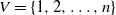
As a simple example where the clustering index is maximized, let $m \geq 2$
,
$m \geq 2$
, $n =2m$
, and consider the graph that is the graph union of an m-null set, and
$n =2m$
, and consider the graph that is the graph union of an m-null set, and $K_m$
(complete graph with m vertices). Figure 1 exemplifies such a construction when
$K_m$
(complete graph with m vertices). Figure 1 exemplifies such a construction when $n=8$
.
$n=8$
.
A graph with eight vertices where ${\mathrm{CI}}_{\alpha} = 8^2/4 = 16$
.
${\mathrm{CI}}_{\alpha} = 8^2/4 = 16$
.

Here, the only contribution to the sum defining ${\mathrm{CI}}_{\alpha}$
is from the cases where a node from
${\mathrm{CI}}_{\alpha}$
is from the cases where a node from $K_m$
and another node from the m-null set are considered. Noting that the clustering coefficient of the node from the m-null set is 0 by definition, the observation that
$K_m$
and another node from the m-null set are considered. Noting that the clustering coefficient of the node from the m-null set is 0 by definition, the observation that ${\mathrm{CI}}_{\alpha}$
takes the value
${\mathrm{CI}}_{\alpha}$
takes the value $n^2/4$
follows immediately.
$n^2/4$
follows immediately.
Another related example is given in Example 2.3 where extremal situations in clustering and degree indices are compared and discussed.
Noting that the observations in Corollary 2.1 can be easily adapted to the degree index, we continue with the following result which provides a way to express the clustering index in terms of the order statistics of the corresponding local clustering coefficients.
Lemma 2.2. (Expression in terms of order statistics.) Let $\mathcal{G} = (V,E)$
be some graph. Order the local clustering coefficients as
$\mathcal{G} = (V,E)$
be some graph. Order the local clustering coefficients as $C_{(1)} \leq C_{(2)} \leq \cdots \leq C_{(n)}$
. Then,
$C_{(1)} \leq C_{(2)} \leq \cdots \leq C_{(n)}$
. Then,
 \begin{align*} \sum_{i < j} |C(i) - C(j)| = \sum_{i = 2}^{n - 1} (2 i - 1 - n) C_{(i)} + (n - 1) (C_{(n)} - C_{(n-1)}).\end{align*}
Proof. Following the proof of Lemma 2.1 with $a_i = C_{(i)} $
gives
$a_i = C_{(i)} $
gives
 \begin{eqnarray*} \sum_{i < j} |C(i) - C(j)| = \sum_{k=2}^n (k - 1)(n+1- k) (C_{(k)}- C_{(k-1)}). \end{eqnarray*}
Expanding the right-hand side as $\sum_{k=2}^n (k - 1)(n+1- k) C_{(k)} - \sum_{k=2}^n (k - 1)(n+1- k) C_{(k-1)}$
, changing the index in the second sum properly, and performing some elementary manipulations yield the result.
$\sum_{k=2}^n (k - 1)(n+1- k) C_{(k)} - \sum_{k=2}^n (k - 1)(n+1- k) C_{(k-1)}$
, changing the index in the second sum properly, and performing some elementary manipulations yield the result.
Let us also examine extremal cases in random graphs. Clearly, any random tree model provides a random graph model for which the lower bound in Corollary 2.1 is achieved. The following example, which is a randomized version of the construction given in Example 2.1, provides a simple random graph model where the upper bound in Corollary 2.1 is achieved asymptotically.
Example 2.2. Begin with two empty sets of nodes $V_1$
and
$V_1$
and $V_2$
at time 0. At each time
$V_2$
at time 0. At each time $t \in \mathbb{N}$
, a newly generated node
$t \in \mathbb{N}$
, a newly generated node $v_t$
is inserted in
$v_t$
is inserted in $V_1$
or
$V_1$
or $V_2$
with probabilities p and
$V_2$
with probabilities p and $1- p$
, respectively. If
$1- p$
, respectively. If $v_t$
is inserted in
$v_t$
is inserted in $V_1$
, we do not attach it to any present nodes. If it is inserted in
$V_1$
, we do not attach it to any present nodes. If it is inserted in $V_2$
, then we attach it to all vertices present in
$V_2$
, then we attach it to all vertices present in $V_2$
. Then, at time
$V_2$
. Then, at time $n \in \mathbb{N}$
, the vertices in
$n \in \mathbb{N}$
, the vertices in $V_1$
form a null graph, and the vertices in
$V_1$
form a null graph, and the vertices in $V_2$
form a complete graph.
$V_2$
form a complete graph.
Letting N be the number of vertices in $V_1$
at time n, N is binomially distributed with parameters n and p, and we have
$V_1$
at time n, N is binomially distributed with parameters n and p, and we have
 \begin{eqnarray*} \mathrm{E} \bigg[ \sum_{i < j} |C(i) - C(j)| \bigg]&\,=\,& \mathrm{E}\bigg[ \mathrm{E} \bigg[ \sum_{i < j} |C(i) - C(j)| \, \bigg| \, N \bigg] \bigg] = \mathrm{E}[N (n - N)] = n \mathrm{E}[N] - \mathrm{E}[N^2] \\ &\,=\,& n^2 p - n p (1- p) - n^2 p^2 = (n^2 -n) p (1 -p). \end{eqnarray*}
When $p = 1/2 $
, we have
$p = 1/2 $
, we have $\mathrm{E} [{\mathrm{CI}}_1 (\mathcal{G}) ]= \tfrac{1}{4} (n^2 -n).$
In particular, for large n,
$\mathrm{E} [{\mathrm{CI}}_1 (\mathcal{G}) ]= \tfrac{1}{4} (n^2 -n).$
In particular, for large n, $\mathrm{E} [{\mathrm{CI}}_1 (\mathcal{G}) ] \approx {n^2}/{4}$
.
$\mathrm{E} [{\mathrm{CI}}_1 (\mathcal{G}) ] \approx {n^2}/{4}$
.
In the following last example, we provide a comparison of the clustering index and the degree index. In particular, we are interested in cases where the degree index is high and the clustering coefficient is low, and vice versa.
Example 2.3. Consider a collection of disjoint polygons, i.e. a graph where each node is contained in a unique polygon. We have $C(i) = 1$
if i is contained in a triangle and
$C(i) = 1$
if i is contained in a triangle and $C(i) = 0$
if i is contained in a polygon other than a triangle. The degree of any node in this graph is 2. Assuming we have k vertices contained in some triangle and
$C(i) = 0$
if i is contained in a polygon other than a triangle. The degree of any node in this graph is 2. Assuming we have k vertices contained in some triangle and $n-k$
vertices contained in a polygon which is not a triangle, we have
$n-k$
vertices contained in a polygon which is not a triangle, we have ${\mathrm{CI}}_{\alpha} = \sum_{1 \leq i < j \leq n} |C(i) - C(j)|^{\alpha} = nk - k^2$
. If n is even, then the maximum is attained when
${\mathrm{CI}}_{\alpha} = \sum_{1 \leq i < j \leq n} |C(i) - C(j)|^{\alpha} = nk - k^2$
. If n is even, then the maximum is attained when $k = n/2$
, which yields
$k = n/2$
, which yields $n^2/4$
. Thus we have found a graph for which the degree index is zero, but the clustering index is
$n^2/4$
. Thus we have found a graph for which the degree index is zero, but the clustering index is $n^2/4$
, the maximal possible value.
$n^2/4$
, the maximal possible value.
Next, we also discuss an example where the clustering index is zero while the degree index $\sum_{1 \leq i < j \leq n} |d_i - d_j|$
is
$\sum_{1 \leq i < j \leq n} |d_i - d_j|$
is ${n^2(n/2-3)}/{4}$
. (Lemma 2.1 can be used to show that the degree index can be at most
${n^2(n/2-3)}/{4}$
. (Lemma 2.1 can be used to show that the degree index can be at most $n^3/4$
. Thus, our example here is off by a factor of
$n^3/4$
. Thus, our example here is off by a factor of $1/2$
, but still demonstrates that the degree index can be very large while the clustering index is zero.)
$1/2$
, but still demonstrates that the degree index can be very large while the clustering index is zero.)
Let n be an integer divisible by 6. Consider a complete graph with $n/2$
vertices, and add
$n/2$
vertices, and add $n/6$
disjoint triangles to the graph. Then
$n/6$
disjoint triangles to the graph. Then $C(i) = 1$
for any i, and so the clustering index is zero. On the other hand,
$C(i) = 1$
for any i, and so the clustering index is zero. On the other hand, $|d_i - d_j| = n/2-3$
if one of the i,j is in our original complete graph while the other belongs to a triangle. Since there are
$|d_i - d_j| = n/2-3$
if one of the i,j is in our original complete graph while the other belongs to a triangle. Since there are $n^2/4$
of these non-zero terms, we conclude
$n^2/4$
of these non-zero terms, we conclude $\sum_{1 \leq i \leq j \leq n} |d_i - d_j| = \frac{n^2(n/2-3)}{4}$
.
$\sum_{1 \leq i \leq j \leq n} |d_i - d_j| = \frac{n^2(n/2-3)}{4}$
.
3. Clustering Index of Erdős–Rényi Graphs
3.1. Sublinearity of $\mathrm{E}[{\mathrm{CI}}_1(\mathcal{G})]$
and
$\mathrm{E}[{\mathrm{CI}}_2(\mathcal{G})]$
$\mathrm{E}[{\mathrm{CI}}_1(\mathcal{G})]$
and
$\mathrm{E}[{\mathrm{CI}}_2(\mathcal{G})]$


In this subsection we focus on the case where $\mathcal{G}$
is an Erdős–Rényi graph, and show that
$\mathcal{G}$
is an Erdős–Rényi graph, and show that $\mathrm{E}[{\mathrm{CI}}_1(\mathcal{G})]$
and
$\mathrm{E}[{\mathrm{CI}}_1(\mathcal{G})]$
and $\mathrm{E}[{\mathrm{CI}}_2(\mathcal{G})]$
are both sublinear. The result for the latter is improved later and, in particular,
$\mathrm{E}[{\mathrm{CI}}_2(\mathcal{G})]$
are both sublinear. The result for the latter is improved later and, in particular, $\mathrm{E}[{\mathrm{CI}}_2(\mathcal{G})]$
will be shown to be bounded by a constant independent of n. We begin with the following proposition concerning the first two moments of the local clustering coefficient.
$\mathrm{E}[{\mathrm{CI}}_2(\mathcal{G})]$
will be shown to be bounded by a constant independent of n. We begin with the following proposition concerning the first two moments of the local clustering coefficient.
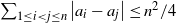
A graph with $d_i = 2$
for any i (hence,
$d_i = 2$
for any i (hence, ${\mathrm{DI}}_{\alpha} = 0$
) but
${\mathrm{DI}}_{\alpha} = 0$
) but ${\mathrm{CI}}_{\alpha}(\mathcal{G}) = n^2/4$
.
${\mathrm{CI}}_{\alpha}(\mathcal{G}) = n^2/4$
.

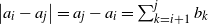
A graph with $C(i) = 1$
for any i (hence,
$C(i) = 1$
for any i (hence, ${\mathrm{CI}}_{\alpha} (\mathcal{G})= 0$
) but
${\mathrm{CI}}_{\alpha} (\mathcal{G})= 0$
) but ${\mathrm{DI}}_{1}(\mathcal{G}) = {n^2(n/2-3)}/{4}$
.
${\mathrm{DI}}_{1}(\mathcal{G}) = {n^2(n/2-3)}/{4}$
.

Proposition 3.1. Let $\mathcal{G} = (V, E)$
be an Erdős–Rényi graph with parameters
$\mathcal{G} = (V, E)$
be an Erdős–Rényi graph with parameters $n \in \mathbb{N}$
and
$n \in \mathbb{N}$
and $p \in (0,1)$
. Let
$p \in (0,1)$
. Let $i \in V$
be any node.
$i \in V$
be any node.
-
(i) We have
In particular,
\begin{align*} \mathrm{E}[C(i)] = p (1 - (1-p)^{n-1} - (n-1)p(1-p)^{n-2}). \end{align*}
$\mathrm{E}[C(i)] \geq p - {D}/{n^2}$
for each n, for some constant D depending on p, but not on n.
-
(ii) We have
where
\begin{align*} | \mathrm{E}[C(i)^2] - p^2 | \leq \frac{D_1}{n^2},\end{align*}
$D_1$
is a positive constant depending on p, but not on n.
-
(iii) We have
${\mathrm{var}}(C(i)) = \mathcal{O}({1}/{n^2}).$


Proof.
-
(i) First, letting
$\phi = \mathrm{P}(d_i \leq 1) = \mathrm{P}(d_i = 0) + \mathrm{P}(d_i = 1) = (1-p)^{n-1} + (n-1)p(1-p)^{n-2}$
, we have (3.1)Now, by the definition of C(i),
\begin{equation}\mathrm{E}[C(i)] = \phi \mathrm{E}[C(i) \mid d_i \leq 1] + (1 - \phi) \mathrm{E}[C(i) \mid d_i \geq 2].\end{equation}
$ \mathrm{E}[C(i) \mid d_i \leq 1] = 0$
. We claim
$ \mathrm{E}[C(i) \mid d_i \geq 2] = p$
. We have where we recall that N(i) is the set of neighbors of node i. Now given
\begin{align*} \mathrm{E}[C(i) \mid d_i \geq 2] &= \mathrm{E}[ \mathrm{E}[ C(i) \mid d_i, d_i \geq 2 ] \mid d_i \geq 2] \\ &= \mathrm{E} \left[ \frac{1}{\binom{d_i}{2}} \mathrm{E} \left[ \sum_{k, \ell \in N(i)} \mathbf{1}(k \leftrightarrow \ell) \,\bigg|\, d_i, d_i \geq 2 \right] \,\bigg|\, d_i \geq 2 \right],\end{align*}
$d_i$
with
$d_i \geq 2$
,
$\sum_{k, \ell \in N(i)} \mathbf{1}(k \leftrightarrow \ell)$
is binomially distributed with parameters
$\binom{d_i}{2}$
and p, whose expectation is
$\binom{d_i}{2} p$
. Therefore, continuing the last observations, we conclude Substituting this into (3.1), we obtain
\begin{align*}\mathrm{E}[C(i) \mid d_i \geq 2] = \mathrm{E} \left[ \frac{1}{\binom{d_i}{2}} \binom{d_i}{2} p \right] = p.\end{align*}
Now, for
\begin{align*}\mathrm{E}[C(i)] &= p (1 - (1-p)^{n-1} - (n-1)p(1-p)^{n-2})\\ &= p - p(1-p)^{n-1} - (n-1)p^2 (1-p)^{n-2}.\end{align*}
$p \in (0,1)$
, the sequence
$p(1-p)^{n-1} + (n-1)p^2 (1-p)^{n-2}$
decays exponentially fast as
$n \rightarrow \infty$
and, thus, it is upper bounded by
$D / n^2$
for some
$D > 0$
. The assertion that
$\mathrm{E}[C(i)] \geq p - {D}/{n^2}$
is now clear.
-
(ii) Note that, in the following, D denotes a constant independent of n that does not necessarily have the same value in its two appearances.


Let $A_i$
be the event that
$A_i$
be the event that $|d_i - (n - 1)p| < n^{2/3}$
. Then by McDiarmid (or Azuma–Hoeffding) inequality [Reference McDiarmid, Habib, McDiarmid, Ramírez-Alfonsín and Reed19],
$|d_i - (n - 1)p| < n^{2/3}$
. Then by McDiarmid (or Azuma–Hoeffding) inequality [Reference McDiarmid, Habib, McDiarmid, Ramírez-Alfonsín and Reed19], $\mathrm{P}(\overline{A_i}) \leq M_1 e^{-M_2 n^{1/3}}$
for some positive constants
$\mathrm{P}(\overline{A_i}) \leq M_1 e^{-M_2 n^{1/3}}$
for some positive constants $M_1, M_2$
independent of n. Using
$M_1, M_2$
independent of n. Using $A_i$
, we now write,
$A_i$
, we now write,
 \begin{align*}\mathrm{E}[C(i)^2] = \mathrm{E}[C(i)^2 \mathbf{1}(A_i)] + \mathrm{E}[C(i)^2 \mathbf{1}(\overline{A_i})].\end{align*}
Let us analyze the two terms on the right-hand side separately. First, focusing on the second term, noting the trivial bound $|C(i)| \leq 1$
, observe that
$|C(i)| \leq 1$
, observe that
 \begin{align*}\mathrm{E}[C(i)^2 \mathbf{1}(\overline{A_i})] \leq \mathrm{P}(\overline{A_i}) \leq M_1 e^{-M_2 n^{1/3}} \leq \frac{D}{n^2}.\end{align*}
Hence, for the second term, we have
 \begin{equation} 0 \leq \mathrm{E}[C(i)^2 \mathbf{1}(\overline{A_i})] \leq \frac{D}{n^2}.\end{equation}
Moving on to the first term, we have
 \begin{eqnarray} \nonumber \mathrm{E}[C(i)^2 \mathbf{1}(A_i)] &\,=&\, \mathrm{E}[\mathrm{E} [C(i)^2 \mathbf{1}(A_i) \mid d_i ]] \nonumber\\ &\,=\,&\, \mathrm{E}\!\left[\mathrm{E} \left[\frac{1}{\binom{d_i}{2}^2} \left( \sum_{\{j,k\} \subset N(i)} \mathbf{1}(j \leftrightarrow k)\right)^2 \mathbf{1}(A_i) {\,\bigg|\,} d_i \right]\right] \nonumber\\ &\,=\,& \, \mathrm{E}\!\left[\frac{\mathbf{1}(A_i)}{\binom{d_i}{2}^2} \mathrm{E} \left[ \sum_{\{j,k\} \subset N(i)} \mathbf{1}(j \leftrightarrow k) + \!\! \sum_{\{j,k\}, \{j',k'\} \subset N(i), \{j,k\} \neq \{j',k'\}} \!\! \mathbf{1}(j \leftrightarrow k, j' \leftrightarrow k') {\,\bigg|\,} d_i \!\right]\right] \nonumber\\ &\,=\,& \, \mathrm{E}\!\left[\frac{\mathbf{1}(A_i)}{\binom{d_i}{2}^2} \left( \binom{d_i}{2} p + \left( \binom{d_i}{2}^2 - \binom{d_i}{2} \right) p^2 \right) \right] \nonumber\\ &\,=\,& \,p^2 \mathrm{E}[\mathbf{1}(A_i)] + (p - p^2) \mathrm{E} \left[ \frac{\mathbf{1}(A_i)}{\binom{d_i}{2}} \right] = p^2 \mathrm{P}(A_i) + (p - p^2) \mathrm{E} \left[ \frac{\mathbf{1}(A_i)}{\binom{d_i}{2}} \right].\end{eqnarray}
Now, when $A_i$
is true,
$A_i$
is true, $(n - 1)p - n^{2 / 3} \leq d_i \leq (n - 1)p + n^{2 / 3}$
. Keeping this in mind, and using the last relation we obtained, we get
$(n - 1)p - n^{2 / 3} \leq d_i \leq (n - 1)p + n^{2 / 3}$
. Keeping this in mind, and using the last relation we obtained, we get
 \begin{align*}\mathrm{E}[C(i)^2 \mathbf{1}(A_i)] \leq p^2 \cdot 1 + \frac{p-p^2}{\binom{(n - 1)p - n^{2 / 3}}{2}} \leq p^2 + \frac{D}{n^2}.\end{align*}
In addition, again by (3.3), we have
 \begin{align*} \mathrm{E}[C(i)^2 \mathbf{1}(A_i)] \geq p^2 \mathrm{P}(A_i) \geq p^2 \big(1 - M_1 e^{-M_2 n^{1/3}}\big) \geq p^2 - \frac{D}{n^2}.\end{align*}
Hence, we conclude that
 \begin{equation} |\mathrm{E}[C(i)^2 \mathbf{1}(A_i)] - p^2 | \leq \frac{D}{n^2}.\end{equation}
Combining (3.2) and (3.4), we arrive at
 \begin{align*}|\mathrm{E}[C(i)^2 - p^2 ] | \leq \frac{D_1}{n^2}, \end{align*}
which holds for every n, where $D_1$
is depending on p, but not on n, as asserted.
$D_1$
is depending on p, but not on n, as asserted.
(iii) Follows immediately from (i) and (ii).
Proposition 3.1 can now be used to show that $\mathrm{E}[{\mathrm{CI}}_1(\mathcal{G})]$
is sublinear.
$\mathrm{E}[{\mathrm{CI}}_1(\mathcal{G})]$
is sublinear.
Theorem 3.1. Let $\mathcal{G}$
be an Erdős–Rényi graph with parameters
$\mathcal{G}$
be an Erdős–Rényi graph with parameters $n \in \mathbb{N}$
and
$n \in \mathbb{N}$
and $p \in (0,1)$
. Then we have
$p \in (0,1)$
. Then we have
 \begin{align*}\mathrm{E}[{\mathrm{CI}}_1(\mathcal{G})] \leq K n, \quad n \geq 1,\end{align*}
where K is a constant depending on p, but not on n.
Proof. Let $i, j \in \mathbb{N}$
. Note that C(i) and C(j) have the same distribution in Erdős–Rényi graphs due to the underlying symmetry. Using this along with the Cauchy–Schwarz inequality, and the previous proposition, we observe
$i, j \in \mathbb{N}$
. Note that C(i) and C(j) have the same distribution in Erdős–Rényi graphs due to the underlying symmetry. Using this along with the Cauchy–Schwarz inequality, and the previous proposition, we observe
 \begin{align*} \mathrm{E}[|C(i) - C(j)|] &= \mathrm{E}[|C(i) - \mathrm{E}[C(i)] + \mathrm{E}[C(j)]- C(j)|] \\ &\leq 2 \mathrm{E} |C(i) - \mathrm{E}|C(i)|| \leq 2 (\mathrm{E} |C(i) - \mathrm{E}|C(i)||^2)^{1/2} = 2 \sqrt{{\mathrm{var}}(C(i))} \leq \frac{D}{n}, \end{align*}
for some constant D. Thus,
 \begin{align*} \mathrm{E}[{\mathrm{CI}}_1(\mathcal{G})] \leq \binom{n}{2} \frac{D}{n} \leq K n. \end{align*}
Noting that the trivial inequality $|C(i) - C(j)|^2 \leq |C(i) - C(j)|$
always holds, one obtains the following corollary.
$|C(i) - C(j)|^2 \leq |C(i) - C(j)|$
always holds, one obtains the following corollary.
Corollary 3.1. In the setting of the previous theorem,
 \begin{align*}\mathrm{E}[{\mathrm{CI}}_2(\mathcal{G})] \leq K n, \quad n \geq 1,\end{align*}
where K is a constant depending on p, but independent of n.
In the next subsection, we show that in the case of Erdős–Rényi graphs for fixed p, $\mathrm{E}[{\mathrm{CI}}_2(\mathcal{G})]$
is indeed bounded by a constant that does not depend on n. Note that our simulation results further suggest that for Erdős–Rényi graphs, the growth of
$\mathrm{E}[{\mathrm{CI}}_2(\mathcal{G})]$
is indeed bounded by a constant that does not depend on n. Note that our simulation results further suggest that for Erdős–Rényi graphs, the growth of ${\mathrm{CI}}_1(\mathcal{G})$
behaves linearly in the number of nodes, and
${\mathrm{CI}}_1(\mathcal{G})$
behaves linearly in the number of nodes, and ${\mathrm{CI}}_2(\mathcal{G})$
converges to a positive constant as the number of nodes increases.
${\mathrm{CI}}_2(\mathcal{G})$
converges to a positive constant as the number of nodes increases.
3.2. Further analysis of
$\mathrm{E}[{\mathrm{CI}}_2(\mathcal{G})]$

Now that we know $\mathrm{E}[{\mathrm{CI}}_2(\mathcal{G})]$
is sublinear via Corollary 3.1 when
$\mathrm{E}[{\mathrm{CI}}_2(\mathcal{G})]$
is sublinear via Corollary 3.1 when $\mathcal{G}$
is an Erdős–Rényi graph, we focus on this expectation in more detail and provide a more precise analysis for this case. This will require understanding of expectations of the form
$\mathcal{G}$
is an Erdős–Rényi graph, we focus on this expectation in more detail and provide a more precise analysis for this case. This will require understanding of expectations of the form $\mathrm{E}[C(i) C(j)]$
for nodes
$\mathrm{E}[C(i) C(j)]$
for nodes $i \neq j$
.
$i \neq j$
.
Proposition 3.2. Let $\mathcal{G}$
be an Erdős–Rényi graph with parameters
$\mathcal{G}$
be an Erdős–Rényi graph with parameters $n \in \mathbb{N}$
and
$n \in \mathbb{N}$
and $p \in (0,1)$
, and i, j be two distinct nodes. Then,
$p \in (0,1)$
, and i, j be two distinct nodes. Then,
 \begin{align*}\mathrm{E}[C(i) C(j)] \geq p^2 - \frac{D_2}{n^2}, \end{align*}
for each n, where $D_2$
is a positive constant depending on p, but not on n.
$D_2$
is a positive constant depending on p, but not on n.
We defer the proof of Proposition 3.2 to the end of this subsection and first discuss the main result.
Theorem 3.2. Let $\mathcal{G}$
be an Erdős–Rényi graph with parameters
$\mathcal{G}$
be an Erdős–Rényi graph with parameters $n \in \mathbb{N}$
and
$n \in \mathbb{N}$
and $p \in (0,1)$
. Then we have
$p \in (0,1)$
. Then we have
 \begin{align*}\mathrm{E}[{\mathrm{CI}}_2(\mathcal{G})] \leq K \end{align*}
for some constant K independent of n.
Proof. By Propositions 3.1 and 3.2, we have
 \begin{align*} \mathrm{E}[{\mathrm{CI}}_2(\mathcal{G})] &= \binom{n}{2} \mathrm{E}[(C(i)-C(j))^2] = \binom{n}{2} \left( \mathrm{E}[C(i)^2] + \mathrm{E}[C(j)^2] - 2\mathrm{E}[C(i)C(j)] \right) \\ &= n(n-1) \big( \mathrm{E}[C(i)^2] - \mathrm{E}[C(i)C(j)] \big) \leq n^2 \left(p^2 + \frac{D_1}{n^2} - p^2 + \frac{D_2}{n^2} \right) = D_1 + D_2 \,=\!:\,K. \end{align*}
Let us now prove Proposition 3.2.
Proof of Proposition
3.2. Recall from the proof of Proposition 3.1 that $A_i$
is the event that
$A_i$
is the event that $|d_i - (n - 1)p| < n^{2/3}$
. Define
$|d_i - (n - 1)p| < n^{2/3}$
. Define $A_j$
similarly. We have
$A_j$
similarly. We have
 \begin{align*}\mathrm{E}[C(i)C(j) ] = \mathrm{E}[C(i)C(j) \mathbf{1}(A_i) \mathbf{1}(A_j) ] + S,\end{align*}
where
 \begin{align*}S= \mathrm{E}[C(i)C(j) \mathbf{1}(A_i) \mathbf{1}(\overline{A_j}) ] + \mathrm{E}[C(i)C(j) \mathbf{1}(\overline{A_i}) \mathbf{1}(A_j) ] + \mathrm{E}[C(i)C(j) \mathbf{1}(\overline{A_i}) \mathbf{1}(\overline{A_j}) ].\end{align*}
Noting that $A_i$
and
$A_i$
and $A_j$
are equally likely, and using trivial upper bound for the clustering coefficients, we see that
$A_j$
are equally likely, and using trivial upper bound for the clustering coefficients, we see that
 \begin{align*}S \leq 3 \mathrm{P}(\overline{A_i}).\end{align*}
Recalling now $\mathrm{P}(\overline{A_i}) \leq M_1 e^{-M_2 n^{1/3}}$
for some constants
$\mathrm{P}(\overline{A_i}) \leq M_1 e^{-M_2 n^{1/3}}$
for some constants $M_1, M_2 > 0$
from the Proof of Proposition 3.1, we conclude that
$M_1, M_2 > 0$
from the Proof of Proposition 3.1, we conclude that
 \begin{align*}S\leq {D}/{n^2}, \quad n \geq 1,\end{align*}
where D is a positive constant independent of n. (Again, D in distinct appearances may denote different constants.) Next, we focus on the estimation of $\mathrm{E}[C(i)C(j) \mathbf{1}(A_i) \mathbf{1}(A_j) ] $
.
$\mathrm{E}[C(i)C(j) \mathbf{1}(A_i) \mathbf{1}(A_j) ] $
.
Let M be the event that the edge between i, j exists. In addition, let $T_i$
and
$T_i$
and $T_j$
denote the number of triangles that contain i and j as a node, respectively. Then
$T_j$
denote the number of triangles that contain i and j as a node, respectively. Then
 \begin{align} \mathrm{E}[C(i)C(j) \mathbf{1}(A_i) \mathbf{1}(A_j) ] &= p \mathrm{E}[C(i)C(j) \mathbf{1}(A_i) \mathbf{1}(A_j) \mid M] + (1 - p) \mathrm{E}[C(i)C(j) \mathbf{1}(A_i) \mathbf{1}(A_j) \mid \overline{M}] \nonumber\\ &= p \mathrm{E} \left[ \frac{\mathbf{1}(A_i) \mathbf{1}(A_j)}{\binom{d_i}{2} \binom{d_j}{2}} \mathrm{E}[T_i T_j {\,\bigg|\,} d_i, d_j, M] {\,\bigg|\,} M\right] \nonumber\\ &\quad + (1- p) \mathrm{E} \left[ \frac{\mathbf{1}(A_i) \mathbf{1}(A_j)}{\binom{d_i}{2} \binom{d_j}{2}} \mathrm{E}[T_i T_j {\,\bigg|\,} d_i, d_j, \overline{M}] {\,\bigg|\,} \overline{M}\right].\end{align}
Now we examine the conditional expectation of $T_i T_j$
given
$T_i T_j$
given $d_i, d_j, M$
and again of
$d_i, d_j, M$
and again of $T_i T_j$
given
$T_i T_j$
given $d_i, d_j, \overline{M}$
in more detail. For this purpose, we decompose
$d_i, d_j, \overline{M}$
in more detail. For this purpose, we decompose $T_i$
and
$T_i$
and $T_j$
as
$T_j$
as
 \begin{align*} T_i = T_{i1} + T_{i2} + T_{i3} \quad \text{and} \quad T_j = T_{j1} + T_{j2} + T_{j3},\end{align*}
where:
-
•
$T_{i1} = T_{j1}$
denotes the number of triangles that have both i and j as vertices; -
•
$T_{i2} = T_{j2}$
denotes the number of edges
$e_{k \ell}$
, with k and
$\ell$
distinct from i and j, and the triangles
$\{i,k,\ell\}$
and
$\{j,k,\ell\}$
both appear in the graph; -
•
$T_{i3}$
and
$T_{j3}$
denote the remaining triangles containing i and j as a node, respectively.


A few observations about this decomposition are in order. First note that conditional on $\overline{M}$
, both
$\overline{M}$
, both $T_{i1}$
and
$T_{i1}$
and $T_{j1} = 0$
. Second, apart from the products
$T_{j1} = 0$
. Second, apart from the products $T_{i1}T_{j1} = T_{i1}^2$
and
$T_{i1}T_{j1} = T_{i1}^2$
and $T_{i2}T_{j2} = T_{i2}^2$
, the products appearing in
$T_{i2}T_{j2} = T_{i2}^2$
, the products appearing in $T_i T_j$
are products of independent random variables given
$T_i T_j$
are products of independent random variables given $M, d_i, d_j$
or
$M, d_i, d_j$
or $\overline{M}, d_i, d_j$
. Hence, to estimate these terms, we can investigate the remainder we obtain from
$\overline{M}, d_i, d_j$
. Hence, to estimate these terms, we can investigate the remainder we obtain from $\mathrm{E}[T_i]\mathrm{E}[T_j]$
in the following way. We have
$\mathrm{E}[T_i]\mathrm{E}[T_j]$
in the following way. We have
 \begin{align} \nonumber \mathrm{E}[T_i T_j \mid M, d_i, d_j] &= \sum_{k=1}^3 \sum_{\ell =1}^3 \mathrm{E}[T_{ik}T_{j\ell} \mid M,d_i,d_j] \nonumber\\[2pt] &= \left(\sum_{(k, \ell) \notin \{(1,1),(2,2)\}} \mathrm{E}[T_{ik} \mid M,d_i,d_j] \mathrm{E}[T_{j\ell} \mid M,d_i,d_j] \right) \nonumber\\[2pt] & \quad + \mathrm{E}[T_{i1}^2 \mid M,d_i,d_j] + \mathrm{E}[T_{i2}^2 \mid M,d_i,d_j] \nonumber\\[2pt] &= \sum_{k=1}^3 \sum_{\ell =1}^3 \mathrm{E}[T_{ik} \mid M,d_i,d_j] \mathrm{E}[T_{j\ell} \mid M,d_i,d_j] \nonumber\\[2pt] & \qquad - \mathrm{E}[T_{i1} \mid M,d_i,d_j] \mathrm{E}[T_{j1} \mid M,d_i,d_j] - \mathrm{E}[T_{i2} \mid M,d_i,d_j] \mathrm{E}[T_{j2} \mid M,d_i,d_j] \nonumber\\[2pt] & \qquad + \mathrm{E}[T_{i1}^2 \mid M,d_i,d_j] + \mathrm{E}[T_{i2}^2 \mid M,d_i,d_j] \nonumber\\[2pt] &= \mathrm{E}[T_{i} \mid M,d_i,d_j] \mathrm{E}[T_{j} \mid M,d_i,d_j] \nonumber\\[2pt] & \qquad + ( \mathrm{E}[T_{i1}^2 \mid M,d_i,d_j] - (\mathrm{E}[T_{i1} \mid M,d_i,d_j] )^2 ) \nonumber\\[2pt] & \qquad + ( \mathrm{E}[T_{i2}^2 \mid M,d_i,d_j] -(\mathrm{E}[T_{i2} \mid M,d_i,d_j] )^2 ) \nonumber\\[2pt] &= \mathrm{E}[T_i \mid M, d_i, d_j] \mathrm{E}[T_j \mid M, d_i, d_j] \nonumber\\[2pt] & \qquad + \mathrm{E}[ T_{i1}^2 - (\mathrm{E}[T_{i1}|M,d_i,d_j])^2|M,d_i, d_j] \nonumber\\[2pt] & \qquad + \mathrm{E}[ T_{i2}^2 - (\mathrm{E}[T_{i2}|M,d_i,d_j])^2|M,d_i, d_j].\end{align}
In addition, recalling that conditional on $\overline{M}$
, both
$\overline{M}$
, both $T_{i1}$
and
$T_{i1}$
and $T_{j1} = 0$
, and following similar steps we obtain
$T_{j1} = 0$
, and following similar steps we obtain
 \begin{equation} \mathrm{E}[T_i T_j \mid \overline{M}, d_i, d_j] = \mathrm{E}[T_i \mid \overline{M}, d_i, d_j] \mathrm{E}[T_j \mid \overline{M}, d_i, d_j] + \mathrm{E}[ T_{i2}^2 - (\mathrm{E}[T_{i2}|\overline{M},d_i,d_j])^2|\overline{M}, d_i, d_j].\end{equation}
Now, note that
 \begin{equation}\mathrm{E}[T_i \mid M, d_i, d_j] = \mathrm{E}[T_i \mid \overline{M}, d_i, d_j] = p \binom{d_i}{2}.\end{equation}
To see this, given the degree $d_i$
of ith node along with
$d_i$
of ith node along with $d_j$
and M, observe that there are
$d_j$
and M, observe that there are $\binom{d_i}{2}$
possible triangles containing node i, and one just needs to count the number of edges between the pairs of neighbors of i to find
$\binom{d_i}{2}$
possible triangles containing node i, and one just needs to count the number of edges between the pairs of neighbors of i to find $T_i$
. Hence, there are
$T_i$
. Hence, there are $\binom{d_i}{2}$
candidates for triangles containing node i, each of which is present with probability p, independent of others. Thus, one has
$\binom{d_i}{2}$
candidates for triangles containing node i, each of which is present with probability p, independent of others. Thus, one has
 \begin{align*}\mathrm{E}[T_i \mid M, d_i, d_j] = p \binom{d_i}{2}.\end{align*}
Noting that given the degree of $d_i$
, the presence or absence of the edge between node i and j does not change the distribution of
$d_i$
, the presence or absence of the edge between node i and j does not change the distribution of $T_i$
, we similarly have
$T_i$
, we similarly have
 \begin{align*}\mathrm{E}[T_i \mid \overline{M}, d_i, d_j] = p \binom{d_i}{2}.\end{align*}
Combining our observations in (3.5), (3.6), (3.7) and (3.8), we obtain,
 \begin{align*} \mathrm{E}[C(i)C(j) \mathbf{1}(A_i) \mathbf{1}(A_j) ] &= p\mathrm{E} \left[ \frac{\mathbf{1}(A_i) \mathbf{1}(A_j)}{\binom{d_i}{2} \binom{d_j}{2}} p^2\binom{d_i}{2} \binom{d_j}{2} \mid M \right] \\[4pt] &+ (1-p)\mathrm{E} \left[ \frac{\mathbf{1}(A_i) \mathbf{1}(A_j)}{\binom{d_i}{2} \binom{d_j}{2}} p^2\binom{d_i}{2} \binom{d_j}{2} \mid \overline{M} \right] \\[4pt] &+ p \mathrm{E} \left[ \frac{\mathbf{1}(A_i) \mathbf{1}(A_j)}{\binom{d_i}{2} \binom{d_j}{2}} \mathrm{E}[ T_{i1}^2 - (\mathrm{E}[T_{i1}|M,d_i,d_j])^2|M,d_i, d_j] \mid M\right] \\[4pt] &+ p \mathrm{E} \left[ \frac{\mathbf{1}(A_i) \mathbf{1}(A_j)}{\binom{d_i}{2} \binom{d_j}{2}} \mathrm{E}[ T_{i2}^2 - (\mathrm{E}[T_{i2}|M,d_i,d_j])^2|M,d_i, d_j] \mid M\right] \\[4pt] &+ (1- p) \mathrm{E} \left[ \frac{\mathbf{1}(A_i) \mathbf{1}(A_j)}{\binom{d_i}{2} \binom{d_j}{2}} \mathrm{E}[ T_{i2}^2 - (\mathrm{E}[T_{i2}|\overline{M},d_i,d_j])^2|\overline{M},d_i, d_j] \mid \overline{M}\right]\!.\end{align*}
The first two terms on the right-hand side simplify to
 \begin{align*}p^2 \left(p \mathrm{E} [ \mathbf{1}(A_i) \mathbf{1}(A_j) \mid M ] + (1-p) \mathrm{E} \left[ \mathbf{1}(A_i) \mathbf{1}(A_j) \mid \overline{M} \right] \right),\end{align*}
which is equal to $p^2\mathrm{E} \left[ \mathbf{1}(A_i) \mathbf{1}(A_j) \right]$
. In addition, all the other terms contain conditional variances of
$p^2\mathrm{E} \left[ \mathbf{1}(A_i) \mathbf{1}(A_j) \right]$
. In addition, all the other terms contain conditional variances of $T_{i1}$
and
$T_{i1}$
and $T_{i2}$
, which are bound to be non-negative random variables and, hence, these terms are non-negative. Thus, we conclude that
$T_{i2}$
, which are bound to be non-negative random variables and, hence, these terms are non-negative. Thus, we conclude that
 \begin{align*} \mathrm{E}[C(i)C(j) \mathbf{1}(A_i) \mathbf{1}(A_j) ] \geq p^2\mathrm{E} \left[ \mathbf{1}(A_i) \mathbf{1}(A_j) \right].\end{align*}
In addition, again recalling from the proof of Proposition 3.1 that $\mathrm{P}(\overline{A_i}) \leq M_1 e^{-M_2 n^{1/3}}$
for some constants
$\mathrm{P}(\overline{A_i}) \leq M_1 e^{-M_2 n^{1/3}}$
for some constants $M_1, M_2$
independent of n, and noting a similar bound holds for
$M_1, M_2$
independent of n, and noting a similar bound holds for $A_j$
, we have
$A_j$
, we have $\mathrm{P}(A_i \cap A_j) \geq 1 - {D}/{n^2}$
for some constant D independent of n. Using this, we reach at
$\mathrm{P}(A_i \cap A_j) \geq 1 - {D}/{n^2}$
for some constant D independent of n. Using this, we reach at
 \begin{align*} \mathrm{E}[C(i)C(j) \mathbf{1}(A_i) \mathbf{1}(A_j) ] \geq p^2 - \frac{D}{n^2},\end{align*}
where D is again independent of n.
Lastly, recalling
 \begin{align*}\mathrm{E}[C(i)C(j) ] = \mathrm{E}[C(i)C(j) \mathbf{1}(A_i) \mathbf{1}(A_j) ] + S, \end{align*}
where $0 \leq S \leq {D}/{n^2}$
, we get
$0 \leq S \leq {D}/{n^2}$
, we get
 \begin{align*}\mathrm{E}[C(i)C(j) ] \geq p^2 - \frac{D_2}{n^2},\end{align*}
as asserted.
4. Degree Index in Erdős–Rényi Graphs
As noted earlier, the degree index (or total degree irregularity) has been introduced and studied previously, but we are not aware of a relevant analysis for random graphs. This section is devoted to such an analysis, and this turns out to be more tractable compared with the clustering index case due to the lack of $\binom{d_i}{2}$
terms in the denominator. We begin the discussion by studying
$\binom{d_i}{2}$
terms in the denominator. We begin the discussion by studying $\mathrm{E}[{\mathrm{DI}}_2(\mathcal{G})]$
.
$\mathrm{E}[{\mathrm{DI}}_2(\mathcal{G})]$
.
Theorem 4.1. For an Erdős–Rényi graph $\mathcal{G}$
with parameters
$\mathcal{G}$
with parameters $n \in \mathbb{N}$
and
$n \in \mathbb{N}$
and $p \in (0,1)$
,
$p \in (0,1)$
,
 \begin{align*}\mathrm{E}[{\mathrm{DI}}_2(\mathcal{G})] = 6\binom{n}{3}p(1-p).\end{align*}
In particular,
 \begin{align*}\frac{\mathrm{E}[{\mathrm{DI}}_2(\mathcal{G})]}{6\binom{n}{3}} = p(1-p),\end{align*}
which is independent of n.
Proof. Let $\mathcal{G}$
be an Erdős–Rényi graph with parameters
$\mathcal{G}$
be an Erdős–Rényi graph with parameters $n \in \mathbb{N}$
and
$n \in \mathbb{N}$
and $p \in (0,1)$
. We are interested in calculating
$p \in (0,1)$
. We are interested in calculating
 \begin{align*}\mathrm{E}\big[(d_i - d_j)^2\big] = 2\mathrm{E}\big[d_i^2\big] - 2\mathrm{E}[d_i d_j].\end{align*}
Let $k = n-2$
for convenience. Denoting the binomial distribution by
$k = n-2$
for convenience. Denoting the binomial distribution by ${\mathrm{Bin}}$
, since
${\mathrm{Bin}}$
, since $d_i \sim {\mathrm{Bin}}(n-1,p) = {\mathrm{Bin}}(k+1,p)$
, we have
$d_i \sim {\mathrm{Bin}}(n-1,p) = {\mathrm{Bin}}(k+1,p)$
, we have
 \begin{align*}\mathrm{E}[d_i^2] = (\mathrm{E}[d_i])^2 + {\mathrm{var}}(d_i) = (n-1)^2p^2 + (n-1)p(1-p) = (k+1)^2p^2 + (k+1)p(1-p).\end{align*}
Next, let us examine $\mathrm{E}[d_i d_j]$
. Let M denote the event that
$\mathrm{E}[d_i d_j]$
. Let M denote the event that $e_{ij}$
appears in the graph. Conditioning on M and
$e_{ij}$
appears in the graph. Conditioning on M and $\overline{M}$
yields
$\overline{M}$
yields
 \begin{align*} \mathrm{E}[d_i d_j] = p\mathrm{E}[d_id_j \mid M] + (1-p) \mathrm{E}[d_id_j \mid \overline{M}]. \end{align*}
If we assume that $e_{ij}$
does not appear in the graph, then the number of possible neighbors of i or j is now
$e_{ij}$
does not appear in the graph, then the number of possible neighbors of i or j is now $n-2$
instead of
$n-2$
instead of $n-1$
. In addition, since we are in the Erdős–Rényi model, the presence of any other edge is independent of the presence of
$n-1$
. In addition, since we are in the Erdős–Rényi model, the presence of any other edge is independent of the presence of $e_{ij}$
. Moreover, apart from whether
$e_{ij}$
. Moreover, apart from whether $e_{ij}$
appears or not,
$e_{ij}$
appears or not, $d_i$
and
$d_i$
and $d_j$
are independent. By the above observations,
$d_j$
are independent. By the above observations, $d_i \mid M$
and
$d_i \mid M$
and $d_j \mid M$
are independent and identically distributed (i.i.d.) with the common distribution
$d_j \mid M$
are independent and identically distributed (i.i.d.) with the common distribution $1 + {\mathrm{Bin}}(n-2,p) = 1 + {\mathrm{Bin}}(k,p)$
. Similarly,
$1 + {\mathrm{Bin}}(n-2,p) = 1 + {\mathrm{Bin}}(k,p)$
. Similarly, $d_i \mid \overline{M}$
and
$d_i \mid \overline{M}$
and $d_j \mid \overline{M}$
are i.i.d. this time with the common distribution
$d_j \mid \overline{M}$
are i.i.d. this time with the common distribution ${\mathrm{Bin}}(n-2,p) = {\mathrm{Bin}}(k,p)$
. Therefore, we have
${\mathrm{Bin}}(n-2,p) = {\mathrm{Bin}}(k,p)$
. Therefore, we have
 \begin{align*} \mathrm{E}[d_i d_j] &= p\mathrm{E}[d_i d_j \mid M] + (1-p)\mathrm{E}[d_i d_j \mid \overline{M}] = p (kp + 1)^2 + (1-p) (kp)^2 \\[4pt] &= k^2p^3 + 2kp^2 + p + k^2p^2 - k^2p^3 = k^2p^2 + 2kp^2 + p, \end{align*}
which implies
 \begin{eqnarray*} \mathrm{E}[d_i^2] - \mathrm{E}[d_i d_j] &\,=\,& (k+1)^2 p^2 + (k+1)p(1-p) - k^2p^2 - 2kp^2 - p \\[4pt] &\,=\,& k^2p^2 + 2kp^2 + p^2 + kp - kp^2 + p - p^2 - k^2p^2 - 2kp^2 - p \\[4pt] &\,=\,& kp - kp^2 = kp(1-p) = (n-2)p(1-p). \end{eqnarray*}
Thus,
 \begin{align*}\mathrm{E}[(d_i-d_j)^2] = 2(n-2)p(1-p).\end{align*}
Recalling that ${\mathrm{DI}}_{2} (\mathcal{G} )= \sum_{1 \leq i < j \leq n} |d_i - d_j|^{2}$
, result follows.
${\mathrm{DI}}_{2} (\mathcal{G} )= \sum_{1 \leq i < j \leq n} |d_i - d_j|^{2}$
, result follows.
Next, we focus on ${\mathrm{DI}}_1(\mathcal{G})$
. In this case a direct computation readily gives
${\mathrm{DI}}_1(\mathcal{G})$
. In this case a direct computation readily gives
 \begin{align*}\mathrm{E}[{\mathrm{DI}}_1(\mathcal{G})] &= \mathrm{E} \left[\sum_{1 \leq i < j \leq n} |d_i - d_j| \right] \nonumber\\[4pt] &= \sum_{\ell =0}^{n-2} \sum_{k=0}^{n-2} |k-\ell| \binom{n-1}{k} \binom{n-1}{\ell} p^k (1-p)^{n-1-k} p^{\ell} (1-p)^{n-1-\ell}.\end{align*}
For clearer expressions, we analyze the symmetric $p=1/2$
case and the general p case separately.
$p=1/2$
case and the general p case separately.
Keeping the notation as above, let us now observe that
 \begin{align*} \mathrm{E}[|d_i - d_j|] = p\mathrm{E}[|d_i - d_j| \mid M] + (1-p) \mathrm{E}[|d_i - d_j| \mid \overline{M}]. \end{align*}
Note that the distribution of $d_i - d_j$
is the same regardless of whether the edge between i and j,
$d_i - d_j$
is the same regardless of whether the edge between i and j, $e_{ij}$
, is present in the graph or not. And since the only dependence between
$e_{ij}$
, is present in the graph or not. And since the only dependence between $d_i$
and
$d_i$
and $d_j$
was a result of
$d_j$
was a result of $e_{ij}$
, we have
$e_{ij}$
, we have
 \begin{align*}\mathrm{E}[|d_i - d_j|] = \mathrm{E}[|B_1 - B_2|],\end{align*}
where $B_1, B_2$
are independent binomial random variables with parameters
$B_1, B_2$
are independent binomial random variables with parameters $n - 2$
and p. For general p case, an easy upper bound on
$n - 2$
and p. For general p case, an easy upper bound on $\mathrm{E}[|d_i - d_j|]$
can be obtained as follows:
$\mathrm{E}[|d_i - d_j|]$
can be obtained as follows:
 \begin{eqnarray*} \mathrm{E}[|d_i - d_j|] &\,=\,& \mathrm{E}|B_1 - B_2| \leq \mathrm{E}|B_1 - (n-2)p| + \mathrm{E}|B_2 - (n-2)p| = 2 \mathrm{E}|B_1 - (n-2)p| \\[4pt] && \leq 2 (\mathrm{E}|B_1 - (n-2)p|^2 )^{1/2} = 2 \sqrt{{\mathrm{var}}(B_1)} = 2 \sqrt{(n-2) p (1-p)}. \end{eqnarray*}
Improving this, one may obtain an exact asymptotic result for $\mathrm{E}[{\mathrm{DI}}_1(\mathcal{G})]$
. This will follow from the following elementary result on the mean absolute difference of binomials.
$\mathrm{E}[{\mathrm{DI}}_1(\mathcal{G})]$
. This will follow from the following elementary result on the mean absolute difference of binomials.
Lemma 4.1. Let $X_n, Y_n$
be independent binomial random variables with parameters
$X_n, Y_n$
be independent binomial random variables with parameters $n \in \mathbb{N}$
and
$n \in \mathbb{N}$
and $p \in (0,1)$
.
$p \in (0,1)$
.
-
(i) If
$p = 1/2$
, then Moreover,
\begin{align*}\mathrm{E}|X_n - Y_n|= \frac{n \binom{2n}{n}}{2^{2n}}.\end{align*}
$\mathrm{E}|X_n - Y_n| \sim \sqrt{{n}/{\pi}}$
, as
$n \rightarrow \infty$
.
-
(ii) For general
$p \in (0,1)$
, we have for every
\begin{align*}\left| \mathrm{E}|X_n - Y_n| - \frac{2}{\sqrt{\pi}} \sqrt{n p (1-p)} \right| \leq D\end{align*}
$n \geq 1$
, where D is a constant depending on p, but not on n. In particular,
$\mathrm{E}|X_n - Y_n| \sim ({2}/{\sqrt{\pi}})\sqrt{n p (1-p)}$
, as
$n \rightarrow \infty$
.


Although the lemma is elementary and there are similar results in the literature (see, for example, [Reference Diaconis and Zabell9]), we were unable to find the exact form used in our case. Therefore, we include the proof of the lemma in the appendix.
Now, given Lemma 4.1, the following result on ${\mathrm{DI}}_1$
follows immediately.
${\mathrm{DI}}_1$
follows immediately.
Theorem 4.2. (i) If $\mathcal{G}$
is an Erdős–Rényi graph with parameters
$\mathcal{G}$
is an Erdős–Rényi graph with parameters $n \in \mathbb{N}$
and
$n \in \mathbb{N}$
and $p = 1/2$
, then
$p = 1/2$
, then
 \begin{align*}\mathrm{E}[{\mathrm{DI}}_1(\mathcal{G})] = \frac{(n-2) \binom{n}{2} \binom{2n-4}{n-2}}{2^{2n-4}}.\end{align*}
In particular, $\mathrm{E}[{\mathrm{DI}}_1(\mathcal{G})] \sim \sqrt{{(n-2)}/{\pi}} \binom{n}{2}$
, as
$\mathrm{E}[{\mathrm{DI}}_1(\mathcal{G})] \sim \sqrt{{(n-2)}/{\pi}} \binom{n}{2}$
, as $n \rightarrow \infty$
.
$n \rightarrow \infty$
.
(ii) If $\mathcal{G}$
is an Erdős–Rényi graph with parameters
$\mathcal{G}$
is an Erdős–Rényi graph with parameters $n \in \mathbb{N}$
and
$n \in \mathbb{N}$
and $p \in (0,1)$
, then
$p \in (0,1)$
, then
 \begin{align*}\mathrm{E}[{\mathrm{DI}}_1(\mathcal{G})] \sim \frac{2}{\sqrt{\pi}} \binom{n}{2} \sqrt{(n-2) p (1 - p)}\end{align*}
as $n \rightarrow \infty$
.
$n \rightarrow \infty$
.
Remark 4.1. One may consider the normalized versions of the degree indices we have studied here in order to be able to do comparisons among distinct random graphs models in a clear way and to make meaningful inferences about the graph properties. Motivated by Theorems 4.1 and 4.2, a natural candidate for the scaled version of the statistic we study is
 \begin{align*}{\mathrm{DI}}_{\alpha}^* = \frac{{\mathrm{DI}}_{\alpha} (\mathcal{G}) }{n^{2 + \alpha /2}}.\end{align*}
Note that in the case of Erdős–Rényi graphs, as $n\rightarrow \infty$
,
$n\rightarrow \infty$
, $\mathrm{E}[{\mathrm{DI}}_{\alpha}^*]$
converges to
$\mathrm{E}[{\mathrm{DI}}_{\alpha}^*]$
converges to $\sqrt{{p(1-p)}/{\pi}}$
and
$\sqrt{{p(1-p)}/{\pi}}$
and $p(1-p)$
for
$p(1-p)$
for $\alpha $
equals 1 and 2, respectively.
$\alpha $
equals 1 and 2, respectively.
In addition, a second natural possible normalization for ${\mathrm{DI}}_{\alpha}(\mathcal{G})$
could be a scaling by
${\mathrm{DI}}_{\alpha}(\mathcal{G})$
could be a scaling by $\binom{n}{2}$
, where n is the number of nodes. However, such a choice does not take
$\binom{n}{2}$
, where n is the number of nodes. However, such a choice does not take $\alpha$
into account, and the scaled limits do not tend to constant values.
$\alpha$
into account, and the scaled limits do not tend to constant values.
5. Monte Carlo Simulations for Other Random Graph Models
The calculations for the degree and clustering indices become more involved when one leaves the framework of Erdős–Rényi random graphs and deals with other models. In this section, we focus on three other random graph models and do a Monte Carlo simulation study for these. The models we are interested in are the Watts–Strogatz model, Barabási–Albert model, and, lastly, random regular graphs. The degree index in random regular graphs is already zero, and one is only interested in the clustering index for this special case.
5.1. Random graph models and implementation
Here, instead of providing a detailed technical background on the random graph models of interest, we briefly discuss the practical aspects of the implementation of Monte Carlo simulations. In particular, we focus on the selection of parameters so that the experiments are performed with matching edge densities for distinct random graph models. Before moving further, let us note that we used the NetworkX module in Python for all the simulations performed in the following. Now, let us review the models under study, keeping in mind that we are willing to have a given edge density $p^* \in (0,1)$
in our simulations.
$p^* \in (0,1)$
in our simulations.
-
1. Erdős–Rényi model. The function erdos_renyi_graph which has parameters n and p as discussed in previous sections produces an Erdős–Rényi graph in NetworkX. One just chooses
$p = p^*$
in order to satisfy the edge density criterion. -
2. Watts–Strogatz model. This model was introduced by Watts and Strogatz in 1998, and it catches certain common properties of real-life complex networks by having the small world property, high clustering, and short average path lengths [Reference Watts and Strogatz25]. The description of watts_strogatz_graph function in NetworkX reference page is as follows:

First create a ring over n nodes. Then each node in the ring is joined to its k nearest neighbors (or $k-1$
neighbors if is odd). Then shortcuts are created by replacing some edges as follows: for each edge (u, v) in the underlying ‘n-ring with k nearest neighbors’ with probability p (rewiring probability) replace it with a new edge (u,w) with uniformly random choice of existing node w.
$k-1$
neighbors if is odd). Then shortcuts are created by replacing some edges as follows: for each edge (u, v) in the underlying ‘n-ring with k nearest neighbors’ with probability p (rewiring probability) replace it with a new edge (u,w) with uniformly random choice of existing node w.
The number of edges in the Watts–Strogatz model is constant and is given by ${nk}/{2}$
. Thus, in order to have the edge density
${nk}/{2}$
. Thus, in order to have the edge density $p^*$
, one needs to have
$p^*$
, one needs to have $p^* = ({{nk}/{2}})/{\binom{n}{2}}$
. Simplifying, we obtain
$p^* = ({{nk}/{2}})/{\binom{n}{2}}$
. Simplifying, we obtain $p^* = {k}/({n - 1})$
. Thus, given
$p^* = {k}/({n - 1})$
. Thus, given $p^*$
and n, one needs to choose k properly so that this criterion is satisfied.
$p^*$
and n, one needs to choose k properly so that this criterion is satisfied.
-
3. Barabási–Albert model. This model, which was introduced by Albert and Barabási in 2002, is a random graph model [Reference Albert and Barabási4] that uses preferential attachment (i.e. higher-degree vertices tend to have even higher degrees) in order to generate scale-free networks. In NetworkX, samples from this model are generated via the barabasi_albert_graph(n, m, seed=None, initial_graph=None) function. The descriptions of the inputs in NetworkX references page are as follows:
-
• n int Number of nodes;
-
• m int Number of edges to attach from a new node to existing nodes;
-
• Initial_graph Graph or None (default) Initial network for Barabási–Albert algorithm; it should be a connected graph for most use cases; a copy of initial_graph is used; if None, starts from a star graph on
$(m+1)$
nodes.
-

In our case, we use the default as the initial graph and so begin with a star on $m+1$
nodes. Now, given the edge density
$m+1$
nodes. Now, given the edge density $p^*$
and the number of nodes n, our goal is to select m so that the resulting Barabási–Albert graph will have approximate edge density
$p^*$
and the number of nodes n, our goal is to select m so that the resulting Barabási–Albert graph will have approximate edge density $p^*$
.
$p^*$
.
Now, since we begin with $m+1$
nodes, the steps required to reach n nodes is
$m+1$
nodes, the steps required to reach n nodes is $N = n - (m+1)$
. Then the number of edges inserted throughout these steps is
$N = n - (m+1)$
. Then the number of edges inserted throughout these steps is $Nm = (n - (m +1))m$
. Thus, also considering the initial nodes present, at the end of the evolution of the graph, we have
$Nm = (n - (m +1))m$
. Thus, also considering the initial nodes present, at the end of the evolution of the graph, we have
 \begin{align*}(n- (m+1) )m + m\end{align*}
many edges, and so the edge density is
 \begin{align*}\frac{(n - (m+1))m + m}{\binom{n}{2}} = \frac{nm - m^2}{\frac{n (n-1)}{2}}.\end{align*}
Hence, we would like to have
 \begin{align*}\frac{nm - m^2}{\frac{n (n-1)}{2}} \approx p^*,\end{align*}
or, rearranging,
 \begin{align*}2m^2 -2n m + n(n-1) p^* \approx 0.\end{align*}
Now the corresponding $\Delta$
is
$\Delta$
is $4n^2 - (4) (2) n(n-1)p^* = 4n^2 - 8 n (n-1)p^*$
. Since
$4n^2 - (4) (2) n(n-1)p^* = 4n^2 - 8 n (n-1)p^*$
. Since $\Delta < 0$
when
$\Delta < 0$
when $p^*$
is large for the number of nodes we intend to simulate, we will only consider the cases
$p^*$
is large for the number of nodes we intend to simulate, we will only consider the cases $p^* = 0.1$
and
$p^* = 0.1$
and $p^*=0.5$
.
$p^*=0.5$
.
When $\Delta > 0$
, the root we use is given by
$\Delta > 0$
, the root we use is given by
 \begin{equation} m^* = \frac{2n - \sqrt{4n^2 - 8 n (n-1)p^*}}{4}. \end{equation}
For example, when $n= 200$
and
$n= 200$
and $p^* = 0.1$
, placing these in the given formula, we find
$p^* = 0.1$
, placing these in the given formula, we find $m^* = 10.501$
, which is rounded to 11. Note that for fixed
$m^* = 10.501$
, which is rounded to 11. Note that for fixed $p^*$
,
$p^*$
, $m^*$
depends linearly on n. In particular, when
$m^*$
depends linearly on n. In particular, when $p^* = 0.5$
,
$p^* = 0.5$
, $m^* \approx {n}/{2}$
and when
$m^* \approx {n}/{2}$
and when $p^* = 0.1$
,
$p^* = 0.1$
, $m^* \approx {n}/{20}$
.
$m^* \approx {n}/{20}$
.
4. Random regular graphs. Random regular graphs are generated using random_regular_ graph(d, n) function in NetworkX. Here, n is the number of nodes and d is the common degree. In this case, to achieve an edge density $p^*$
, one needs to have
$p^*$
, one needs to have
 \begin{align*} p^* = \frac{\frac{nd}{2}}{\binom{n}{2}}, \end{align*}
which can be rewritten as $p^* = {d}/({n-1})$
. Thus, given n and
$p^* = {d}/({n-1})$
. Thus, given n and $p^*$
, we choose d appropriately to achieve the given edge density.
$p^*$
, we choose d appropriately to achieve the given edge density.
5.2. Results for the clustering index
Now we are ready to present the simulation results. In each fixed selection of parameters, 120–600 sample graphs of each model were generated for varying node counts, and these were averaged to approximate the value of interest. For each plot, the number of nodes was chosen from the set $\{20, 40,\ldots, 380\}$
, and the resulting averages were linearly interpolated. Note that the rewiring probability in the Watts–Strogatz model does not affect the number of vertices nor the edge density; hence, in each of our simulations, we examined Watts–Strogatz graphs with rewiring probabilities of 0.1, 0.3, 0.5, 0.7, and 0.9. In many of our simulations, Barabási–Albert graph and some of the Watts–Strogatz graphs had growth rates significantly larger than the others; thus, we have created additional plots to better examine the remaining graph models in all our plots.
$\{20, 40,\ldots, 380\}$
, and the resulting averages were linearly interpolated. Note that the rewiring probability in the Watts–Strogatz model does not affect the number of vertices nor the edge density; hence, in each of our simulations, we examined Watts–Strogatz graphs with rewiring probabilities of 0.1, 0.3, 0.5, 0.7, and 0.9. In many of our simulations, Barabási–Albert graph and some of the Watts–Strogatz graphs had growth rates significantly larger than the others; thus, we have created additional plots to better examine the remaining graph models in all our plots.
Figure 4 contains our results for ${\mathrm{CI}}_1$
. Note that these plots are for the Barabási–Albert model where the parameter
${\mathrm{CI}}_1$
. Note that these plots are for the Barabási–Albert model where the parameter $m = m^*$
is chosen according to (5.1) in order to satisfy the edge density condition. In particular, this is in contrast to the standard Barabási–Albert model where m is a fixed positive integer. One would naturally obtain a distinct growth rate for the standard case. We give a more detailed relevant discussion later when we focus on the degree index.
$m = m^*$
is chosen according to (5.1) in order to satisfy the edge density condition. In particular, this is in contrast to the standard Barabási–Albert model where m is a fixed positive integer. One would naturally obtain a distinct growth rate for the standard case. We give a more detailed relevant discussion later when we focus on the degree index.
Average ${\mathrm{CI}}_1$
values of the Erdős–Rényi graph, Barabási–Albert graph, random regular graph, and Watts–Strogatz graphs with edge densities 0.1 and 0.5.
${\mathrm{CI}}_1$
values of the Erdős–Rényi graph, Barabási–Albert graph, random regular graph, and Watts–Strogatz graphs with edge densities 0.1 and 0.5.

Our expectation from our theoretical findings was that the growth of ${\mathrm{CI}}_1$
for Erdős–Rényi graphs was sublinear in n, which is verified in our simulation. One would also expect that, as the rewiring probability increases, the Watts–Strogatz graphs exhibit increasingly similar behavior to Erdős–Rényi graphs in terms of clustering, which seems to be the case.
${\mathrm{CI}}_1$
for Erdős–Rényi graphs was sublinear in n, which is verified in our simulation. One would also expect that, as the rewiring probability increases, the Watts–Strogatz graphs exhibit increasingly similar behavior to Erdős–Rényi graphs in terms of clustering, which seems to be the case.
In Figure 5, we include the comparison of ${\mathrm{CI}}_2$
for the four models of interest. In the case of Erdős–Rényi, we showed that this index is upper bounded by a constant independent of the number of nodes and we conjecture that it is indeed also lower bounded by a constant. This is indeed the case according to our simulations, where
${\mathrm{CI}}_2$
for the four models of interest. In the case of Erdős–Rényi, we showed that this index is upper bounded by a constant independent of the number of nodes and we conjecture that it is indeed also lower bounded by a constant. This is indeed the case according to our simulations, where ${\mathrm{CI}}_2$
can be observed to approach
${\mathrm{CI}}_2$
can be observed to approach ${2(1-p)(1-p^2)}/{p}$
as n increases. Watts–Strogatz graphs with low rewiring probability and the Barabási–Albert model again dominate the others in this case. In addition, as in the case of
${2(1-p)(1-p^2)}/{p}$
as n increases. Watts–Strogatz graphs with low rewiring probability and the Barabási–Albert model again dominate the others in this case. In addition, as in the case of ${\mathrm{CI}}_1$
, we observe that as the rewiring probability increases,
${\mathrm{CI}}_1$
, we observe that as the rewiring probability increases, ${\mathrm{CI}}_2$
of the Watts–Strogatz model approaches that of Erdős–Rényi model.
${\mathrm{CI}}_2$
of the Watts–Strogatz model approaches that of Erdős–Rényi model.
Average ${\mathrm{CI}}_2$
values of the Erdős–Rényi graph, Barabási–Albert graph, random regular graph, and Watts–Strogatz graphs with edge densities 0.1 and 0.5.
${\mathrm{CI}}_2$
values of the Erdős–Rényi graph, Barabási–Albert graph, random regular graph, and Watts–Strogatz graphs with edge densities 0.1 and 0.5.

It is also interesting in Figure 5 to note that many of our random graphs seem to exhibit a peaking behavior around 40–60 nodes when the edge density is 0.1. We think that the appearance of these peaks is a result of an equilibrium of two opposing effects:
-
• as n increases, the number of terms appearing in the sum
${\mathrm{CI}}_2$
also increases; -
• as n increases, the variance of the distribution of local clustering coefficients decreases.

When the edge density is 0.5, the Barabási–Albert model with $m = m^*$
again dominates the others; it seems to exhibit
$m = m^*$
again dominates the others; it seems to exhibit $\Theta(n^2)$
growth while the others are sublinear. The Watts–Strogatz model with lower rewiring probabilities again follows the Barabási–Albert case in the ranking.
$\Theta(n^2)$
growth while the others are sublinear. The Watts–Strogatz model with lower rewiring probabilities again follows the Barabási–Albert case in the ranking.
For the Barabási–Albert model with $m=m^*$
, when the edge density is 0.5, both
$m=m^*$
, when the edge density is 0.5, both ${\mathrm{CI}}_1$
and
${\mathrm{CI}}_1$
and ${\mathrm{CI}}_2$
seem to be of order
${\mathrm{CI}}_2$
seem to be of order $n^2$
. This is caused by the vastly different clustering behavior of the leaves of the initial star graph and the other nodes. Since
$n^2$
. This is caused by the vastly different clustering behavior of the leaves of the initial star graph and the other nodes. Since $m \approx n/2$
in this case, the initial star graph has
$m \approx n/2$
in this case, the initial star graph has $m-1 \approx n/2 -1$
leaves. Our simulation results show that, when n is large, the local clustering coefficients of these leaves are significantly higher compared with the clustering coefficients of the other nodes on average. This causes
$m-1 \approx n/2 -1$
leaves. Our simulation results show that, when n is large, the local clustering coefficients of these leaves are significantly higher compared with the clustering coefficients of the other nodes on average. This causes $\mathrm{E}[{\mathrm{CI}}_1] \geq K_1 \binom{n}{2}$
and
$\mathrm{E}[{\mathrm{CI}}_1] \geq K_1 \binom{n}{2}$
and $\mathrm{E}[{\mathrm{CI}}_2] \geq K_2 \binom{n}{2}$
for positive constants
$\mathrm{E}[{\mathrm{CI}}_2] \geq K_2 \binom{n}{2}$
for positive constants $K_1, K_2$
.
$K_1, K_2$
.
5.3. Results for the degree index
In this subsection, we focus on the degree index and compare ${\mathrm{DI}}_1$
and
${\mathrm{DI}}_1$
and ${\mathrm{DI}}_2$
for the same four random graph models again for varying values of the number of nodes.
${\mathrm{DI}}_2$
for the same four random graph models again for varying values of the number of nodes.
Figure 6 is for ${\mathrm{DI}}_1$
and the edge density
${\mathrm{DI}}_1$
and the edge density $0.1$
. Note that again there are two versions corresponding to each edge density due to the domination of the Barabási–Albert model with
$0.1$
. Note that again there are two versions corresponding to each edge density due to the domination of the Barabási–Albert model with $m = m^*$
. In particular, those on the right do not contain the case for the Barabási–Albert model. Figure 7 is for
$m = m^*$
. In particular, those on the right do not contain the case for the Barabási–Albert model. Figure 7 is for ${\mathrm{DI}}_1$
and the edge density
${\mathrm{DI}}_1$
and the edge density $0.5$
.
$0.5$
.
Average ${\mathrm{DI}}_1$
values of the Erdős–Rényi graph, Barabási–Albert graph, random regular graph, and Watts–Strogatz graphs with edge density 0.1.
${\mathrm{DI}}_1$
values of the Erdős–Rényi graph, Barabási–Albert graph, random regular graph, and Watts–Strogatz graphs with edge density 0.1.

Average ${\mathrm{DI}}_1$
values of the Erdős–Rényi graph, Barabási–Albert graph, random regular graph, and Watts–Strogatz graphs with edge density 0.5.
${\mathrm{DI}}_1$
values of the Erdős–Rényi graph, Barabási–Albert graph, random regular graph, and Watts–Strogatz graphs with edge density 0.5.

We see that as in the case of the clustering index, the small world model behaves similarly to Erdős–Rényi as the rewiring probability increases. In order to examine the behaviors for different models in more detail, we also include the log–log plots for the graphs on the left in Figures 6 and 7.
The log–log plot clearly indicates that the growth of $\mathrm{E}[{\mathrm{DI}}_1]$
for the preferential attachment model we consider is of higher order than the growth of other cases. The simulations we have and the heuristic arguments we use suggest that the growth rate in this case is of order
$\mathrm{E}[{\mathrm{DI}}_1]$
for the preferential attachment model we consider is of higher order than the growth of other cases. The simulations we have and the heuristic arguments we use suggest that the growth rate in this case is of order $\Theta(n^3)$
, which is strictly larger than that for Erdős–Rényi graphs (which is
$\Theta(n^3)$
, which is strictly larger than that for Erdős–Rényi graphs (which is $\Theta(n^{5/2})$
). However, note that the Barabási–Albert model we consider is different from the standard Barabási–Albert model in the following sense. Here, in order to have a fixed edge density for comparison among distinct models, the corresponding parameter m increases as a function of n as explained in Section 5.1; see (5.1). Thus, if we consider the standard Barabási–Albert model where m is fixed, then we would obtain a different behavior. Indeed, we were informed by an anonymous reviewer that the maximal degree in the standard Barabási–Albert model is of order
$\Theta(n^{5/2})$
). However, note that the Barabási–Albert model we consider is different from the standard Barabási–Albert model in the following sense. Here, in order to have a fixed edge density for comparison among distinct models, the corresponding parameter m increases as a function of n as explained in Section 5.1; see (5.1). Thus, if we consider the standard Barabási–Albert model where m is fixed, then we would obtain a different behavior. Indeed, we were informed by an anonymous reviewer that the maximal degree in the standard Barabási–Albert model is of order $\sqrt{n}$
; see, for example, [Reference van der Hofstad13, p. 280]. From this, one immediately obtains a trivial upper bound of order
$\sqrt{n}$
; see, for example, [Reference van der Hofstad13, p. 280]. From this, one immediately obtains a trivial upper bound of order $n^{5/2}$
for
$n^{5/2}$
for ${\mathrm{DI}}_1$
for fixed m. To have a better understanding, we also simulated the standard Barabási–Albert model. Figure 9 contains the corresponding log–log plot.
${\mathrm{DI}}_1$
for fixed m. To have a better understanding, we also simulated the standard Barabási–Albert model. Figure 9 contains the corresponding log–log plot.
The log–log plots for the $\mathrm{DI}_1$
values of the Erdős–Rényi graph, modified Barabási–Albert graph, and Watts–Strogatz graphs with edge densities 0.1 and 0.5.
$\mathrm{DI}_1$
values of the Erdős–Rényi graph, modified Barabási–Albert graph, and Watts–Strogatz graphs with edge densities 0.1 and 0.5.

The log–log plots for the ${\mathrm{DI}}_1$
and
${\mathrm{DI}}_1$
and ${\mathrm{DI}}_2$
values of the Barabási–Albert graphs with
${\mathrm{DI}}_2$
values of the Barabási–Albert graphs with $m \in \{1,2,3,5,10\}$
, where m denotes the number of edges to attach from a new node to existing nodes. The number of nodes is from 500 to 6000, with increments of 500.
$m \in \{1,2,3,5,10\}$
, where m denotes the number of edges to attach from a new node to existing nodes. The number of nodes is from 500 to 6000, with increments of 500.

The plots in Figure 9 and the related slope calculations suggest that $\mathrm{E}[{\mathrm{DI}}_1] = \Theta(n^2)$
when m is fixed. This seems natural since in this case the degrees of most nodes tend to be small and close to each other, which then causes
$\mathrm{E}[{\mathrm{DI}}_1] = \Theta(n^2)$
when m is fixed. This seems natural since in this case the degrees of most nodes tend to be small and close to each other, which then causes ${\mathrm{DI}}_1$
to be small. On the other hand, in the Barabási–Albert model with
${\mathrm{DI}}_1$
to be small. On the other hand, in the Barabási–Albert model with $m = m^*$
, (5.1) gives
$m = m^*$
, (5.1) gives $m^* \sim C n$
for some
$m^* \sim C n$
for some $C \in (0,1)$
. In turn, this causes a significant number of nodes to have degrees comparable to n and a remarkable number of nodes to have significantly smaller degrees, with the result that
$C \in (0,1)$
. In turn, this causes a significant number of nodes to have degrees comparable to n and a remarkable number of nodes to have significantly smaller degrees, with the result that $\mathrm{E}[|d_i - d_j|]$
is of order n and
$\mathrm{E}[|d_i - d_j|]$
is of order n and $\mathrm{E}[{\mathrm{DI}}_1]$
is of order
$\mathrm{E}[{\mathrm{DI}}_1]$
is of order $n^3$
.
$n^3$
.
For the ${\mathrm{DI}}_2$
case, the simulation results are summarized in Figures 10 and 11. The observations here are similar to the
${\mathrm{DI}}_2$
case, the simulation results are summarized in Figures 10 and 11. The observations here are similar to the ${\mathrm{DI}}_1$
case, and we do not provide the details of these to avoid repetition.
${\mathrm{DI}}_1$
case, and we do not provide the details of these to avoid repetition.
Average ${\mathrm{DI}}_2$
values of the Erdős–Rényi graph, modified Barabási–Albert graph, random regular graph, and Watts–Strogatz graphs with edge density 0.1.
${\mathrm{DI}}_2$
values of the Erdős–Rényi graph, modified Barabási–Albert graph, random regular graph, and Watts–Strogatz graphs with edge density 0.1.

Average ${\mathrm{DI}}_2$
values of the Erdős–Rényi graph, modified Barabási–Albert graph, random regular graph, and Watts–Strogatz graphs with edge density 0.5.
${\mathrm{DI}}_2$
values of the Erdős–Rényi graph, modified Barabási–Albert graph, random regular graph, and Watts–Strogatz graphs with edge density 0.5.

We close this section by noting that we also analyzed the log–log plot for the case ${\mathrm{DI}}_2$
for the Barabási–Albert model with
${\mathrm{DI}}_2$
for the Barabási–Albert model with $m = m^*$
, and that the related observations suggest
$m = m^*$
, and that the related observations suggest $\mathrm{E}[{\mathrm{DI}}_2] = \Theta(n^4)$
.
$\mathrm{E}[{\mathrm{DI}}_2] = \Theta(n^4)$
.
6. Conclusion
In this paper, in addition to the well-known degree index (or irregularity), we have introduced the concept of the clustering index and studied the first moment of both in a random graph framework. Focusing on Erdős–Rényi graphs and the degree case, we were able to obtain either exact or asymptotic expressions for the expected degree indices of interest. Regarding the clustering index case, we have obtained a linear upper bound for $\mathrm{E}[{\mathrm{CI}}_1(\mathcal{G})]$
, and also have shown that
$\mathrm{E}[{\mathrm{CI}}_1(\mathcal{G})]$
, and also have shown that $\mathrm{E}[{\mathrm{CI}}_2(\mathcal{G})]$
is bounded above by a constant independent of n. Although we had a theoretical and simulation-based related analysis for random graphs, we have not done a detailed study of the indices of interest for real-life complex networks and we intend to do so in a subsequent work.
$\mathrm{E}[{\mathrm{CI}}_2(\mathcal{G})]$
is bounded above by a constant independent of n. Although we had a theoretical and simulation-based related analysis for random graphs, we have not done a detailed study of the indices of interest for real-life complex networks and we intend to do so in a subsequent work.
One main motivation for studying these indices in our case is their possible use in artificial intelligence classification algorithms as features. Characteristics such as average clustering and the average degree are already used in various such problems, and we intend to do an experimental study in future work to see whether the use of degree and clustering indices provides improvements in performance in classification problems. A second related path is in the field of finance, more particularly in the detection of financial crises. In a recent work [Reference Huang, Deng, Yang, Yang and Cao14], it was argued that a certain graph irregularity measure, namely the Laplace energy, can be used to detect economic crises. Recently, we did some preliminary experiments to see whether the indices introduced in this paper could also be considered for such purposes. The initial analysis indicated that both are useful in this direction, but that the results for degree index are more statistically significant. We plan to conduct a rigorous analysis on whether degree and clustering indices (as certain types of network irregularities) can also be considered as a precursor of financial crises in upcoming work.
The last direction we are willing to follow is in computing the exact asymptotics of ${\mathrm{CI}}_1$
and
${\mathrm{CI}}_1$
and ${\mathrm{CI}}_2 $
in the case of Erdős–Rényi graphs. For example, focusing on
${\mathrm{CI}}_2 $
in the case of Erdős–Rényi graphs. For example, focusing on ${\mathrm{CI}}_2$
, we were able to obtain a constant upper bound, and simulations suggested that this index indeed behaves like a constant as the number of nodes increases. It would be interesting to verify this convergence theoretically.
${\mathrm{CI}}_2$
, we were able to obtain a constant upper bound, and simulations suggested that this index indeed behaves like a constant as the number of nodes increases. It would be interesting to verify this convergence theoretically.
Appendix. Proof of Lemma 4.1.
-
(i) Let
$X_n, Y_n$
be independent binomial random variables with parameters n and
$1/2$
. We claim that
$\mathrm{E}|X_n - Y_n| = {n \binom{2n}{n}}/{2^{2n}}$
. For this purpose, letting
$Z_n$
be an independent binomial random variable with parameters n and
$1/2$
, observe that where
\begin{align*}|X_n - Y_n| =_d |X_n - n + Z_n | = |X_n +Z_n - n| = |T_n - n|,\end{align*}
$T_n = X_n + Z_n$
is a binomial random variable with parameters 2n and
$1/2$
. Then, We have
\begin{align*}\mathrm{P} (|X_n - Y_n| = k) = \mathrm{P} (|T_n -n| = k) = 2 \mathrm{P} (T_n = n + k) = \binom{2n}{n + k} \frac{1}{2^{2n - 1}}.\end{align*}
The assertion that
\begin{eqnarray*} \mathrm{E}|X_n - Y_n| = \sum_{k = 0}^n k \binom{2n}{n + k} \frac{1}{2^{2n - 1}} &\,=\,& \frac{1}{2^{2n - 1}} \sum_{k= 1}^n (k - n + n) \binom{2n}{n + k} \\[4pt] &\,=\,& \frac{1}{2^{2n - 1}} \sum_{k= 1}^n (n + k) \binom{2n}{n + k} - \frac{1}{2^{2n - 1}} \sum_{k= 1}^n n \binom{2n}{n + k} \\[4pt] &\,=\,& \frac{2n}{2^{2n - 1}} \sum_{k=1}^n \binom{2n - 1}{n + k -1} - \frac{n}{2^{2n - 1} } \sum_{k = 1}^n \binom{2n}{n + k} \\[4pt] &\,=\,& \frac{2n}{2^{2n - 1}} \frac{2^{2n - 1}}{2} - \frac{n}{2^{2n - 1}} \left( \frac{2^n - \binom{2n}{n}}{2} \right) = \frac{n \binom{2n}{n}}{2^{2n}}. \end{eqnarray*}
$\mathrm{E}|X_n - Y_n| \sim \sqrt{\frac{n}{\pi}}$
,
$n \rightarrow \infty$
, now follows from Stirling’s approximation.
-
(ii) Let
$Z_1, Z_2$
be independent standard normal random variables. We denote the Wasserstein distance between the distributions by
$d_W$
. Now, letting
$\mu_n = \mathrm{E}[X_n]$
and
$\sigma_n^2 = {\mathrm{var}}(X_n)$
, recall that for some constant D independent of n (See, for example, [Reference Ross21]). We in particular have
\begin{align*}d_W \left( \frac{X_n - \mu_n}{\sigma_n} , Z_1\right) &\,:\!=\, \sup \left\{ \mathrm{E} \left| h \left(\frac{X_n - \mu_n}{\sigma_n} \right) - h(Z_1) \right|\,:\, h\,:\, \mathbb{R} \rightarrow \mathbb{R}, |h(x) - h(y)| \right.\\[4pt] &\left. \leq |x - y| \right\} \leq \frac{D}{\sqrt{n}},\end{align*}
With previous observations, and together with triangle inequality, this gives
\begin{align*}\mathrm{E} \left| \frac{X_n - \mu_n}{\sigma_n} - Z_1 \right| \leq \frac{D}{\sqrt{n}}.\end{align*}
\begin{eqnarray*} \mathrm{E}|X_n - Y_n| &\,=\,& \sigma_n \left|\frac{X_n - \mu_n}{\sigma_n} - Z_1 + Z_1 - Z_2 + Z_2 - \frac{Y_n - \mu_n}{\sigma_n} \right| \\[4pt] &\leq& 2 \sigma_n \mathrm{E} \left|\frac{X_n - \mu_n}{\sigma_n} - Z_1\right| + \sigma_n \mathrm{E}|Z_1 - Z_2| \\[4pt] &\leq& \frac{2 C \sigma_n}{\sqrt{n}} + \sigma_n \mathrm{E}|Z_1 - Z_2| = \mathcal{O}(1) + \sigma_n \mathrm{E}|Z_1 - Z_2|. \end{eqnarray*}
In addition, using the triangle inequality in an appropriate way,
\begin{eqnarray*} \mathrm{E}|X_n - Y_n | &\,=\,& \sigma_n \left| \left( \frac{X_n - \mu_n}{\sigma_n} - Z_1 \right) + (Z_1 - Z_2) + \left(Z_2 - \frac{Y_n - \mu_n}{\sigma_n} \right)\right| \\[4pt] &\,=\,& \sigma_n \mathrm{E}|a + b + c| \geq \sigma_n \mathrm{E}|b| - \sigma_n \mathrm{E}|a| - \sigma_n \mathrm{E}|c| \\[4pt] &\,=\,& \sigma_n \mathrm{E}|Z_1 - Z_2| - 2 \sigma_n \mathrm{E}\bigg|\frac{X_n - \mu_n}{\sigma_n} - Z_1\bigg| \\[4pt] &\geq&\sigma_n \mathrm{E}|Z_1 - Z_2| - \frac{2 \sigma_n D}{\sqrt{n}} = \mathcal{O}(1) + \sigma_n \mathrm{E}|Z_1 - Z_2|. \end{eqnarray*}
Thus,
$({1}/{\sigma_n}) \mathrm{E} |X_n - Y_n |$
converges to
$\mathrm{E}|Z_1 - Z_2|$
. The result now follows since
$\mathrm{E}|Z_1 - Z_2| = 2 / \sqrt{\pi}$
.


Acknowledgements
We would like to thank the anonymous reviewers whose suggestions and corrections improved the paper significantly. Parts of this paper were completed at the Nesin Mathematics Village, the authors would like to thank Nesin Mathematics Village for their kind hospitality.
Funding information
The first author was supported by the BAGEP Award of the Science Academy, Turkey.
Competing interests
There were no competing interests to declare which arose during the preparation or publication process of this article.

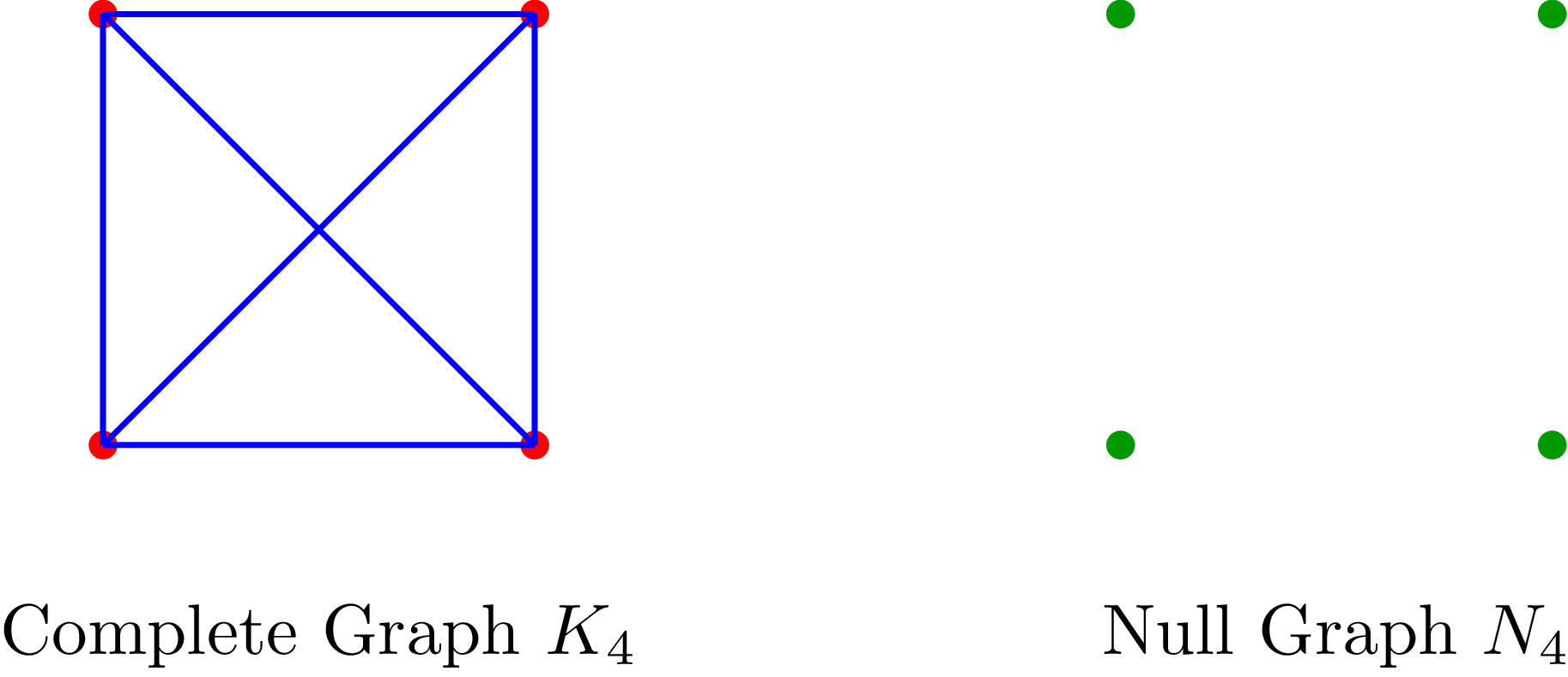

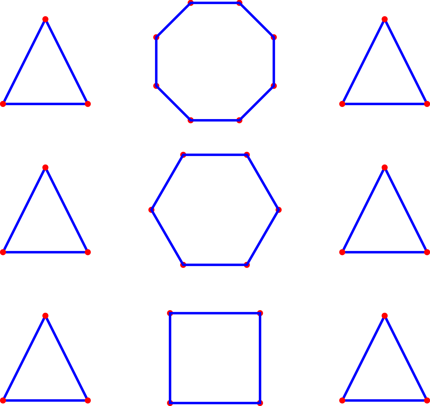


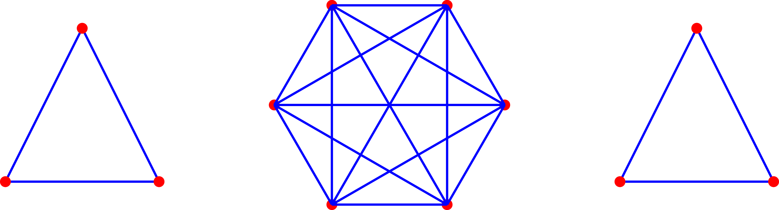


 Open access