


1 Introduction
A comprehensive modelling of magnetized plasmas and of their multi-scale dynamics is an outstanding challenge in laboratory, astrophysical and space plasma research. In particular, given that direct numerical simulations are nowadays the main tool to address such complex dynamics, finding a compromise between an exhaustive theoretical model and its actual implementation represents a major goal for computational plasma physics.
A kinetic model based on the full Vlasov–Maxwell system of equations would need to be solved in a six-dimensional phase space (three real-space and three velocity-space dimensions), resolving length and time scales that typically span over several orders of magnitude. For this reason, fully kinetic simulations that adopt realistic parameters and/or complex geometries are still far from being realizable because of their colossal computational cost. Moreover, there is overwhelming difficulty in constructing an analytical description of Vlasov equilibria in realistic settings. In fact, the few existing examples typically consider very simplified cases (e.g. uniform and homogeneous magnetic field and/or only periodic functions) and still one cannot fully constrain the resulting velocity profiles beforehand and/or provide those equilibria without appealing to a numerical solution of the problem (see, e.g. Cai, Storey & Neubert Reference Cai, Storey and Neubert1990; Attico & Pegoraro Reference Attico and Pegoraro1999; Mahajan & Hazeltine Reference Mahajan and Hazeltine2000; Bobrova et al. Reference Bobrova, Bulanov, Sakai and Sugiyama2001; Malara, Pezzi & Valentini Reference Malara, Pezzi and Valentini2018).
On the other hand, a model based on a fluid treatment such as the magnetohydrodynamic (MHD) equations neglects most of the characteristic length and time scales inherent to a kinetic description of the plasma dynamics and only needs to be solved in real space. The MHD description thus represents the simplest viable approach, which nevertheless has led to many fundamental theoretical results (e.g. Chapman & Ferraro Reference Chapman and Ferraro1930; Ferraro Reference Ferraro1937; Alfvén Reference Alfvén1942; Lüst & Schlüter Reference Lüst and Schlüter1954; Chandrasekhar Reference Chandrasekhar1956; Shafranov Reference Shafranov1958; Grad Reference Grad1960; Taylor Reference Taylor1974). Furthermore, in the last two decades, we have been able to afford well-resolved MHD global simulations providing useful insights (e.g. Groth et al. Reference Groth, De Zeeuw, Gombosi and Powell2000; Siscoe et al. Reference Siscoe, Crooker, Erickson, Sonnerup, Siebert, Weimer, White and Maynard2000; Jia et al. Reference Jia, Hansen, Gombosi, Kivelson, Tóth, Dezeeuw and Ridley2012, Reference Jia, Slavin, Gombosi, Daldorff, Tóth and van der Holst2015; Merkin, Lyon & Claudepierre Reference Merkin, Lyon and Claudepierre2013; Liu et al. Reference Liu, Lu, Wang, Kabin, Zhao, Wang, Han, Wang and Zhao2015; Dong et al. Reference Dong, Lingam, Ma and Cohen2017; Sorathia et al. Reference Sorathia, Merkin, Ukhorskiy, Mauk and Sibeck2017). However, in a real system, the nonlinear plasma dynamics would naturally develop small scales and bring the effects associated with the neglected kinetic scales back to light, and so a MHD description eventually breaks down. Moreover, accounting for the leading kinetic effects may already be necessary to implement a correct initial plasma equilibrium, in order to avoid uncontrolled and spurious readjustments that can affect the subsequent dynamics or to explain certain features of the system under consideration (e.g. Cerri et al. Reference Cerri, Henri, Califano, Del Sarto, Faganello and Pegoraro2013; Henri et al. Reference Henri, Cerri, Califano, Pegoraro, Rossi, Faganello, Šebek, Trávníček, Hellinger and Frederiksen2013).
The fully kinetic and MHD descriptions actually represent the two extremes of a wide variety of plasma models. There are a large number of approaches that try to bridge the above antipodes in different ways: from the one side, by simplifying a fully kinetic description based on the dismissal of presumably unimportant effects; from the opposite side, by gradually including more and more kinetic effects within a fluid framework. The former class of models are usually referred to as ‘reduced-kinetic models’, such as the gyrokinetic (GK) (Brizard & Hahm Reference Brizard and Hahm2007) and the hybrid Vlasov–Maxwell (HVM) (Valentini et al. Reference Valentini, Trávníček, Califano, Hellinger and Mangeney2007) approximations; the latter are known as ‘extended-fluid models’, in which kinetic effects are gradually included in a fluid description. This is the case, for instance, when retaining finite-Larmor-radius (FLR) corrections (Roberts & Taylor Reference Roberts and Taylor1962; Macmahon Reference Macmahon1965), or when including the effect of linear Landau damping (Landau Reference Landau1946) by modelling it with a so-called Landau-fluid (LF) closure (e.g. Hammett & Perkins Reference Hammett and Perkins1990). These two aspects can also be both included within a single framework, such as in the so-called finite-Larmor-radius Landau-fluid (FLRLF) model (Sulem & Passot Reference Sulem and Passot2015). However, within the range of validity defined by each model’s assumption (‘ordering’), reduced-kinetic models still unavoidably face the curse of high dimensionality, and so extended-fluid models still represent an attractive choice when seeking a compromise between kinetic and fluid descriptions.
The need to extend a standard fluid description of a collisionless plasma to include at least these effects related to a non-gyrotropic pressure tensor is particularly evident when a sheared flow is present: in the collisionless regime, due to FLR effects, the pressure tensor is indeed strongly coupled to the shear flow and they interact over very short time scales (Cerri Reference Cerri2012; Cerri et al.
Reference Cerri, Henri, Califano, Del Sarto, Faganello and Pegoraro2013, Reference Cerri, Pegoraro, Califano, Del Sarto and Jenko2014; Del Sarto, Pegoraro & Califano Reference Del Sarto, Pegoraro and Califano2016; Del Sarto, Pegoraro & Tenerani Reference Del Sarto, Pegoraro and Tenerani2017; Del Sarto & Pegoraro Reference Del Sarto and Pegoraro2018). This is exactly the case of the low-latitude boundary layer (LLBL) between the solar-wind flow and the Earth’s magnetosphere, where the velocity shear drives the Kelvin–Helmholtz instability (KHI) that generates the observed large-scale ‘MHD’ vortices (see, e.g. Faganello & Califano Reference Faganello and Califano2017 and references therein). In such a region, in addition to the vortex dynamics that naturally develops fluctuations on length scales comparable to (or even smaller than) the ion gyroradius $\unicode[STIX]{x1D71A}_{i}$
(or the ion inertial length
$\unicode[STIX]{x1D71A}_{i}$
(or the ion inertial length $d_{i}$
), the ‘large-scale’ equilibrium fields and the sheared flow itself vary over typical length scales
$d_{i}$
), the ‘large-scale’ equilibrium fields and the sheared flow itself vary over typical length scales $L_{0}$
that do not exceed the ion characteristic scales by a large amount, and so ‘
$L_{0}$
that do not exceed the ion characteristic scales by a large amount, and so ‘ $\unicode[STIX]{x1D71A}_{i}/L_{0}$
corrections’ cannot be completely neglected. So far, such a system has been modelled by means of one-dimensional isotropic MHD equilibrium configurations that ensure the total pressure balance, i.e. a balance between the thermal and magnetic scalar pressures of the two plasmas without involving the properties of the background sheared flow. However, as soon as FLR effects and/or the full ion pressure tensor are taken into account, the shear-flow properties enter the pressure-balance conditions and the simple isotropic MHD configurations are generally no longer an equilibrium (Cerri Reference Cerri2012; Cerri et al.
Reference Cerri, Henri, Califano, Del Sarto, Faganello and Pegoraro2013, Reference Cerri, Pegoraro, Califano, Del Sarto and Jenko2014). As a result, the system naturally develops shear-driven anisotropies (e.g. De Camillis et al.
Reference De Camillis, Cerri, Califano and Pegoraro2016; Del Sarto et al.
Reference Del Sarto, Pegoraro and Califano2016; Del Sarto & Pegoraro Reference Del Sarto and Pegoraro2018). This is important for (at least) two practical reasons. First, a difficulty arises when comparing the linear evolution of the KHI using fluid and kinetic models. As discussed in Henri et al. (Reference Henri, Cerri, Califano, Pegoraro, Rossi, Faganello, Šebek, Trávníček, Hellinger and Frederiksen2013), in which the same isotropic MHD configuration was adopted as an initial condition for simulations using different plasma models (namely, MHD, two-fluid, hybrid and full Particle-In-Cell (PIC)), it was found that violent and uncontrolled readjustments were injecting large-amplitude fluctuations into the system (see also Del Sarto et al.
Reference Del Sarto, Pegoraro and Tenerani2017) and changing the configuration on top of which the instability develops (see also Nakamura, Hasegawa & Shinohara Reference Nakamura, Hasegawa and Shinohara2010). Therefore, these spurious effects would partially mask the actual kinetic effects on the KHI and make a genuine comparison difficult. Secondly, using ten years of observations made by the Cluster satellites, Haaland et al. (Reference Haaland, Reistad, Tenfjord, Gjerloev, Maes, Dekeyser, Maggiolo, Anekallu and Dorville2014) have recently highlighted that the Earth’s magnetopause exhibits a current structure that is more complex than the simple MHD layer described by Chapman & Ferraro (Reference Chapman and Ferraro1930), as well as a clear asymmetry between the dusk and the dawn sides. In addition to the implications for the current system of a planet magnetosphere, these ion-kinetic effects can indeed cause the asymmetric development of KHI at the dawn and the dusk sides of such magnetosphere, as well as other non-ideal effects (e.g. Nagano Reference Nagano1978; Huba Reference Huba1996; Terada, Machida & Shinagawa Reference Terada, Machida and Shinagawa2002; Nakamura et al.
Reference Nakamura, Hasegawa and Shinohara2010; Henri et al.
Reference Henri, Califano, Faganello and Pegoraro2012; Masters et al.
Reference Masters, Achilleos, Cutler, Coates, Dougherty and Jones2012; Sundberg et al.
Reference Sundberg, Boardsen, Slavin, Anderson, Korth, Zurbuchen, Raines and Solomon2012; Taylor et al.
Reference Taylor, Hasegawa, Lavraud, Phan, Escoubet, Dunlop, Bogdanova, Borg, Volwerk and Berchem2012; Delamere et al.
Reference Delamere, Wilson, Eriksson and Bagenal2013; Paral & Rankin Reference Paral and Rankin2013; Haaland et al.
Reference Haaland, Reistad, Tenfjord, Gjerloev, Maes, Dekeyser, Maggiolo, Anekallu and Dorville2014; Johnson, Wing & Delamere Reference Johnson, Wing and Delamere2014; Liljeblad et al.
Reference Liljeblad, Sundberg, Karlsson and Kullen2014; Walsh et al.
Reference Walsh, Haaland, Forsyth, Keesee, Kissinger, Li, Runov, Soucek, Walsh and Wing2014; Gershman et al.
Reference Gershman, Raines, Slavin, Zurbuchen, Sundberg, Boardsen, Anderson, Korth and Solomon2015; Gingell, Sundberg & Burgess Reference Gingell, Sundberg and Burgess2015; De Camillis et al.
Reference De Camillis, Cerri, Califano and Pegoraro2016).
$\unicode[STIX]{x1D71A}_{i}/L_{0}$
corrections’ cannot be completely neglected. So far, such a system has been modelled by means of one-dimensional isotropic MHD equilibrium configurations that ensure the total pressure balance, i.e. a balance between the thermal and magnetic scalar pressures of the two plasmas without involving the properties of the background sheared flow. However, as soon as FLR effects and/or the full ion pressure tensor are taken into account, the shear-flow properties enter the pressure-balance conditions and the simple isotropic MHD configurations are generally no longer an equilibrium (Cerri Reference Cerri2012; Cerri et al.
Reference Cerri, Henri, Califano, Del Sarto, Faganello and Pegoraro2013, Reference Cerri, Pegoraro, Califano, Del Sarto and Jenko2014). As a result, the system naturally develops shear-driven anisotropies (e.g. De Camillis et al.
Reference De Camillis, Cerri, Califano and Pegoraro2016; Del Sarto et al.
Reference Del Sarto, Pegoraro and Califano2016; Del Sarto & Pegoraro Reference Del Sarto and Pegoraro2018). This is important for (at least) two practical reasons. First, a difficulty arises when comparing the linear evolution of the KHI using fluid and kinetic models. As discussed in Henri et al. (Reference Henri, Cerri, Califano, Pegoraro, Rossi, Faganello, Šebek, Trávníček, Hellinger and Frederiksen2013), in which the same isotropic MHD configuration was adopted as an initial condition for simulations using different plasma models (namely, MHD, two-fluid, hybrid and full Particle-In-Cell (PIC)), it was found that violent and uncontrolled readjustments were injecting large-amplitude fluctuations into the system (see also Del Sarto et al.
Reference Del Sarto, Pegoraro and Tenerani2017) and changing the configuration on top of which the instability develops (see also Nakamura, Hasegawa & Shinohara Reference Nakamura, Hasegawa and Shinohara2010). Therefore, these spurious effects would partially mask the actual kinetic effects on the KHI and make a genuine comparison difficult. Secondly, using ten years of observations made by the Cluster satellites, Haaland et al. (Reference Haaland, Reistad, Tenfjord, Gjerloev, Maes, Dekeyser, Maggiolo, Anekallu and Dorville2014) have recently highlighted that the Earth’s magnetopause exhibits a current structure that is more complex than the simple MHD layer described by Chapman & Ferraro (Reference Chapman and Ferraro1930), as well as a clear asymmetry between the dusk and the dawn sides. In addition to the implications for the current system of a planet magnetosphere, these ion-kinetic effects can indeed cause the asymmetric development of KHI at the dawn and the dusk sides of such magnetosphere, as well as other non-ideal effects (e.g. Nagano Reference Nagano1978; Huba Reference Huba1996; Terada, Machida & Shinagawa Reference Terada, Machida and Shinagawa2002; Nakamura et al.
Reference Nakamura, Hasegawa and Shinohara2010; Henri et al.
Reference Henri, Califano, Faganello and Pegoraro2012; Masters et al.
Reference Masters, Achilleos, Cutler, Coates, Dougherty and Jones2012; Sundberg et al.
Reference Sundberg, Boardsen, Slavin, Anderson, Korth, Zurbuchen, Raines and Solomon2012; Taylor et al.
Reference Taylor, Hasegawa, Lavraud, Phan, Escoubet, Dunlop, Bogdanova, Borg, Volwerk and Berchem2012; Delamere et al.
Reference Delamere, Wilson, Eriksson and Bagenal2013; Paral & Rankin Reference Paral and Rankin2013; Haaland et al.
Reference Haaland, Reistad, Tenfjord, Gjerloev, Maes, Dekeyser, Maggiolo, Anekallu and Dorville2014; Johnson, Wing & Delamere Reference Johnson, Wing and Delamere2014; Liljeblad et al.
Reference Liljeblad, Sundberg, Karlsson and Kullen2014; Walsh et al.
Reference Walsh, Haaland, Forsyth, Keesee, Kissinger, Li, Runov, Soucek, Walsh and Wing2014; Gershman et al.
Reference Gershman, Raines, Slavin, Zurbuchen, Sundberg, Boardsen, Anderson, Korth and Solomon2015; Gingell, Sundberg & Burgess Reference Gingell, Sundberg and Burgess2015; De Camillis et al.
Reference De Camillis, Cerri, Califano and Pegoraro2016).
The aim of the present work is to show how the non-ideal behaviour of the Chapman–Ferraro layer could be qualitatively understood in terms of a one-dimensional equilibrium of the shear-flow layer within an extended-fluid model that includes first-order ion-FLR corrections. The great simplicity of the treatment presented here allows us to derive analytical equilibrium profiles in which the ion-kinetic effects can be clearly identified. Therefore this study is meant to be a first step – a sort of ‘proof of concept’ – towards the identification of the effects possibly leading to the observed behaviour of the low-latitude magnetopause layer, rather than an exhaustive description of the actual system. In order to achieve a quantitative modelling of the global magnetopause current system within this (or a more comprehensive) extended-fluid model, a numerical approach to the solution of the full three-dimensional problem would likely be required.
The remainder of this paper is organized as follows. In § 2 we describe the extended two-fluid (eTF) model of Cerri et al. (Reference Cerri, Henri, Califano, Del Sarto, Faganello and Pegoraro2013) and we outline the procedure for the derivation of the equilibrium profiles (the actual derivation of a general family of solutions for the shear-flow boundary layer equilibrium is provided in appendix A); consequences for shear-flow instabilities, agyrotropy and links to turbulent environments are highlighted in §§ 2.3–2.5. In § 3 we show how these profiles can qualitatively explain the observed non-ideal behaviour of the LLBL between the solar wind and the Earth’s magnetosphere. Finally, in § 4 conclusions are drawn. Additionally, explicit considerations on the symmetries of the FLR expansion and on its convergence to a full pressure tensor case are reported in appendices B and C, respectively.
2 The extended two-fluid (eTF) model
Here, we consider a non-relativistic quasi-neutral proton–electron plasma ( $n_{\text{p}}\simeq n_{\text{e}}\equiv n$
) in the limit of massless electrons,
$n_{\text{p}}\simeq n_{\text{e}}\equiv n$
) in the limit of massless electrons, $m_{\text{e}}/m_{\text{p}}\rightarrow 0$
. The model includes the Hall and the electron pressure terms in the generalized Ohm’s law, as well as dynamic equations for the gyrotropic pressures of both species and first-order FLR corrections to the protons’ pressure tensorFootnote
1
. The fluid hierarchy is closed with a double-adiabatic approximation, i.e. by neglecting the heat fluxes,
$m_{\text{e}}/m_{\text{p}}\rightarrow 0$
. The model includes the Hall and the electron pressure terms in the generalized Ohm’s law, as well as dynamic equations for the gyrotropic pressures of both species and first-order FLR corrections to the protons’ pressure tensorFootnote
1
. The fluid hierarchy is closed with a double-adiabatic approximation, i.e. by neglecting the heat fluxes, $q_{\Vert }=0$
and
$q_{\Vert }=0$
and $q_{\bot }=0$
. Such assumption is indeed justified within a finite-but-small Larmor-radius expansion and on time scales much longer than the ion cyclotron time scale,
$q_{\bot }=0$
. Such assumption is indeed justified within a finite-but-small Larmor-radius expansion and on time scales much longer than the ion cyclotron time scale, $\unicode[STIX]{x1D70C}/L\sim \unicode[STIX]{x1D714}/\unicode[STIX]{x1D6FA}\sim \unicode[STIX]{x1D700}\ll 1$
, where
$\unicode[STIX]{x1D70C}/L\sim \unicode[STIX]{x1D714}/\unicode[STIX]{x1D6FA}\sim \unicode[STIX]{x1D700}\ll 1$
, where $\unicode[STIX]{x1D70C}$
is the thermal Larmor radius,
$\unicode[STIX]{x1D70C}$
is the thermal Larmor radius, $L$
is the typical length scale of variation for macroscopic quantities and
$L$
is the typical length scale of variation for macroscopic quantities and $\unicode[STIX]{x1D6FA}$
is the cyclotron frequency (see Cerri et al.
Reference Cerri, Henri, Califano, Del Sarto, Faganello and Pegoraro2013, for explicit equations and further details about the eTF model ordering). In fact, by neglecting gradients in the direction of the magnetic field (
$\unicode[STIX]{x1D6FA}$
is the cyclotron frequency (see Cerri et al.
Reference Cerri, Henri, Califano, Del Sarto, Faganello and Pegoraro2013, for explicit equations and further details about the eTF model ordering). In fact, by neglecting gradients in the direction of the magnetic field ( $\boldsymbol{b}\boldsymbol{\cdot }\unicode[STIX]{x1D735}=\unicode[STIX]{x1D735}_{\Vert }=0$
; see appendix A), the expressions for the perpendicular heat fluxes (see, e.g. Braginskii Reference Braginskii1965; Ramos Reference Ramos2008) would give a second-order contribution which is ordered out in the eTF modelFootnote
2
. In this model, the thermal pressure tensor of the protons and of the electrons,
$\boldsymbol{b}\boldsymbol{\cdot }\unicode[STIX]{x1D735}=\unicode[STIX]{x1D735}_{\Vert }=0$
; see appendix A), the expressions for the perpendicular heat fluxes (see, e.g. Braginskii Reference Braginskii1965; Ramos Reference Ramos2008) would give a second-order contribution which is ordered out in the eTF modelFootnote
2
. In this model, the thermal pressure tensor of the protons and of the electrons, $\unicode[STIX]{x1D72B}_{\text{p}}$
and
$\unicode[STIX]{x1D72B}_{\text{p}}$
and $\unicode[STIX]{x1D72B}_{\text{e}}$
respectively, are written as
$\unicode[STIX]{x1D72B}_{\text{e}}$
respectively, are written as
 $$\begin{eqnarray}\displaystyle & \displaystyle \unicode[STIX]{x1D72B}_{\text{p}}=p_{\Vert \text{p}}\boldsymbol{b}\boldsymbol{b}+p_{\bot \text{p}}\unicode[STIX]{x1D749}+\unicode[STIX]{x03C0}_{\text{p}}^{(1)}, & \displaystyle\end{eqnarray}$$
 $$\begin{eqnarray}\displaystyle & \displaystyle \unicode[STIX]{x1D72B}_{\text{e}}=p_{\Vert \text{e}}\boldsymbol{b}\boldsymbol{b}+p_{\bot \text{e}}\unicode[STIX]{x1D749}, & \displaystyle\end{eqnarray}$$
where $\boldsymbol{b}\equiv \boldsymbol{B}/|\boldsymbol{B}|$
is the magnetic-field unit vector,
$\boldsymbol{b}\equiv \boldsymbol{B}/|\boldsymbol{B}|$
is the magnetic-field unit vector, $\unicode[STIX]{x1D749}\equiv \unicode[STIX]{x1D644}-\boldsymbol{b}\boldsymbol{b}$
is the projector onto the plane perpendicular to
$\unicode[STIX]{x1D749}\equiv \unicode[STIX]{x1D644}-\boldsymbol{b}\boldsymbol{b}$
is the projector onto the plane perpendicular to $\boldsymbol{B}$
and
$\boldsymbol{B}$
and $p_{\Vert \unicode[STIX]{x1D6FC}}$
and
$p_{\Vert \unicode[STIX]{x1D6FC}}$
and $p_{\bot \unicode[STIX]{x1D6FC}}$
are the gyrotropic thermal pressures of the
$p_{\bot \unicode[STIX]{x1D6FC}}$
are the gyrotropic thermal pressures of the $\unicode[STIX]{x1D6FC}$
species parallel and perpendicular to the magnetic field, respectively (Chew, Goldberger & Low Reference Chew, Goldberger and Low1956). In (2.1),
$\unicode[STIX]{x1D6FC}$
species parallel and perpendicular to the magnetic field, respectively (Chew, Goldberger & Low Reference Chew, Goldberger and Low1956). In (2.1), $\unicode[STIX]{x03C0}_{\text{p}}^{(1)}$
is a traceless symmetric tensor taking into account first-order FLR corrections to the gyrotropic proton pressure (also known as gyroviscous tensor). Neglecting the heat fluxes, a general formulation for the gyroviscous tensor components can be written as (Macmahon Reference Macmahon1965; Schekochihin et al.
Reference Schekochihin, Cowley, Rincon and Rosin2010; Sulem & Passot Reference Sulem and Passot2015)
$\unicode[STIX]{x03C0}_{\text{p}}^{(1)}$
is a traceless symmetric tensor taking into account first-order FLR corrections to the gyrotropic proton pressure (also known as gyroviscous tensor). Neglecting the heat fluxes, a general formulation for the gyroviscous tensor components can be written as (Macmahon Reference Macmahon1965; Schekochihin et al.
Reference Schekochihin, Cowley, Rincon and Rosin2010; Sulem & Passot Reference Sulem and Passot2015)
 $$\begin{eqnarray}\unicode[STIX]{x03C0}_{\text{p},ij}^{(1)}=\frac{p_{\bot \text{p}}}{4\unicode[STIX]{x1D6FA}_{c\text{p}}}(\unicode[STIX]{x1D716}_{ilm}b_{l}S_{mk}H_{kj}-H_{ik}\unicode[STIX]{x1D716}_{jlm}S_{kl}b_{m})+\frac{2(p_{\bot \text{p}}-p_{\Vert \text{p}})}{\unicode[STIX]{x1D6FA}_{c\text{p}}}(b_{i}w_{j}+b_{j}w_{i}),\end{eqnarray}$$
where $\unicode[STIX]{x1D6FA}_{c\text{p}}=eB/m_{\text{p}}c$
is the proton gyro-frequency,
$\unicode[STIX]{x1D6FA}_{c\text{p}}=eB/m_{\text{p}}c$
is the proton gyro-frequency, $\unicode[STIX]{x1D716}_{ijk}$
is the completely antisymmetric Levi-Civita tensor, and we have introduced
$\unicode[STIX]{x1D716}_{ijk}$
is the completely antisymmetric Levi-Civita tensor, and we have introduced $S_{ij}\equiv \unicode[STIX]{x2202}_{i}u_{\text{p},j}+\unicode[STIX]{x2202}_{j}u_{\text{p},i}$
,
$S_{ij}\equiv \unicode[STIX]{x2202}_{i}u_{\text{p},j}+\unicode[STIX]{x2202}_{j}u_{\text{p},i}$
, $H_{ij}\equiv \unicode[STIX]{x1D6FF}_{ij}+3b_{i}b_{j}$
and
$H_{ij}\equiv \unicode[STIX]{x1D6FF}_{ij}+3b_{i}b_{j}$
and $w_{i}\equiv \unicode[STIX]{x1D716}_{ijk}(\unicode[STIX]{x1D735}_{\Vert }u_{\text{p},j})b_{k}$
, with
$w_{i}\equiv \unicode[STIX]{x1D716}_{ijk}(\unicode[STIX]{x1D735}_{\Vert }u_{\text{p},j})b_{k}$
, with $\unicode[STIX]{x1D735}_{\Vert }\equiv \boldsymbol{b}\boldsymbol{\cdot }\unicode[STIX]{x1D735}$
. Note that the above formulation automatically takes into account for the asymmetry due to the magnetic field direction with respect to the vorticity (see also appendix B and Cerri et al.
Reference Cerri, Henri, Califano, Del Sarto, Faganello and Pegoraro2013, for explicit symmetry considerations).
$\unicode[STIX]{x1D735}_{\Vert }\equiv \boldsymbol{b}\boldsymbol{\cdot }\unicode[STIX]{x1D735}$
. Note that the above formulation automatically takes into account for the asymmetry due to the magnetic field direction with respect to the vorticity (see also appendix B and Cerri et al.
Reference Cerri, Henri, Califano, Del Sarto, Faganello and Pegoraro2013, for explicit symmetry considerations).
2.1 Shear-flow layer equilibrium with FLR
Within this model, we now outline the derivation of equilibrium profiles for a one-dimensional velocity-shear layer separating, for instance, two different plasmas. The explicit derivation of this class of analytical solutions that generalize the results provided in Cerri et al. (Reference Cerri, Henri, Califano, Del Sarto, Faganello and Pegoraro2013) and that include a much wider range of configurations of interest for what concerns magnetospheric observations will be provided in appendix A. The goal is to provide an equilibrium configuration with FLR corrections for the flank magnetopause, and to discuss the implications on the low-latitude boundary layer (LLBL) profiles. For the sake of simplicity, here we consider the one-dimensional equilibrium problem, which can be seen as a local approximation of the LLBL. A global treatment of the magnetospheric structure should take into account curvature terms, as well as possible gradients parallel to the magnetic field and compressible flows. This may need to include additional equilibrium conditions that involve all the gyroviscous components and eventually to go beyond the simple adiabatic FLR treatment presented here by, for instance, including heat fluxes (see, e.g. Sulem & Passot Reference Sulem and Passot2015; Del Sarto & Pegoraro Reference Del Sarto and Pegoraro2018).
We consider a given $x$
-dependent incompressible MHD flow in the
$x$
-dependent incompressible MHD flow in the $y$
–
$y$
– $z$
plane,
$z$
plane,
 $$\begin{eqnarray}\boldsymbol{u}=u_{y}(x)\boldsymbol{e}_{y}+u_{z}(x)\boldsymbol{e}_{z},\quad \unicode[STIX]{x1D735}\boldsymbol{\cdot }\boldsymbol{u}=0,\end{eqnarray}$$
such that it becomes constant at the boundaries (i.e. we consider a localized velocity-shear layer). The magnetic field also lies on the $y$
–
$y$
– $z$
plane,
$z$
plane,
 $$\begin{eqnarray}\boldsymbol{B}(x)=B_{y}(x)\boldsymbol{e}_{y}+B_{z}(x)\boldsymbol{e}_{z}.\end{eqnarray}$$
We further simplify the problem by assuming a polytropic relation for the thermal pressuresFootnote 3 . This assumption is not strictly necessary in order to derive the equilibrium, but it is useful for providing density and temperature profiles from the obtained pressure profiles. In general, the equilibrium for this configuration is found by imposing total pressure balance:
 $$\begin{eqnarray}\frac{\text{d}}{\text{d}x}[\unicode[STIX]{x1D72B}_{\text{p}}(x)+\unicode[STIX]{x1D72B}_{\text{e}}(x)+\unicode[STIX]{x1D72B}_{\text{B}}(x)]=0,\end{eqnarray}$$
where $\unicode[STIX]{x1D72B}_{\text{B}}\equiv (B^{2}/8\unicode[STIX]{x03C0})\unicode[STIX]{x1D644}-\boldsymbol{B}\boldsymbol{B}$
is the magnetic pressure tensor (
$\unicode[STIX]{x1D72B}_{\text{B}}\equiv (B^{2}/8\unicode[STIX]{x03C0})\unicode[STIX]{x1D644}-\boldsymbol{B}\boldsymbol{B}$
is the magnetic pressure tensor ( $\unicode[STIX]{x1D644}$
being the identity tensor). Within an (anisotropic) MHD model of plasma, the shear flow does not play a role in the equilibrium profile. In fact, when
$\unicode[STIX]{x1D644}$
being the identity tensor). Within an (anisotropic) MHD model of plasma, the shear flow does not play a role in the equilibrium profile. In fact, when $\unicode[STIX]{x03C0}_{\text{p}}^{(1)}$
is neglected, the equilibrium condition for the above configuration simply consists of a balance between the magnetic pressure,
$\unicode[STIX]{x03C0}_{\text{p}}^{(1)}$
is neglected, the equilibrium condition for the above configuration simply consists of a balance between the magnetic pressure, $P_{B}(x)=B^{2}(x)/8\unicode[STIX]{x03C0}$
, and the perpendicular thermal pressures,
$P_{B}(x)=B^{2}(x)/8\unicode[STIX]{x03C0}$
, and the perpendicular thermal pressures, $P_{\bot }(x)=p_{\bot \text{p}}(x)+p_{\bot \text{e}}(x)$
. In particular, that includes the widely adopted uniform and homogeneous plasma configuration, namely
$P_{\bot }(x)=p_{\bot \text{p}}(x)+p_{\bot \text{e}}(x)$
. In particular, that includes the widely adopted uniform and homogeneous plasma configuration, namely $p_{\bot \unicode[STIX]{x1D6FC}}=p_{\Vert \unicode[STIX]{x1D6FC},0}$
,
$p_{\bot \unicode[STIX]{x1D6FC}}=p_{\Vert \unicode[STIX]{x1D6FC},0}$
, $p_{\bot \unicode[STIX]{x1D6FC}}=p_{\bot \unicode[STIX]{x1D6FC},0}$
,
$p_{\bot \unicode[STIX]{x1D6FC}}=p_{\bot \unicode[STIX]{x1D6FC},0}$
, $B_{y}=B_{0y}$
and
$B_{y}=B_{0y}$
and $B_{z}=B_{0z}$
, that is not allowed anymore when FLR corrections (or the full pressure-tensor equations) are included in the fluid description (Cerri Reference Cerri2012; Cerri et al.
Reference Cerri, Henri, Califano, Del Sarto, Faganello and Pegoraro2013, Reference Cerri, Pegoraro, Califano, Del Sarto and Jenko2014). In general, the solution of the MHD equilibrium condition is completely described by the chosen magnetic profile in (2.5), which determines all the profiles of the other relevant quantities. Let us now consider the changes of a given MHD equilibrium profile that are induced by a velocity shear of the type described above when first-order FLR corrections are taken into account. In this case, the only component of
$B_{z}=B_{0z}$
, that is not allowed anymore when FLR corrections (or the full pressure-tensor equations) are included in the fluid description (Cerri Reference Cerri2012; Cerri et al.
Reference Cerri, Henri, Califano, Del Sarto, Faganello and Pegoraro2013, Reference Cerri, Pegoraro, Califano, Del Sarto and Jenko2014). In general, the solution of the MHD equilibrium condition is completely described by the chosen magnetic profile in (2.5), which determines all the profiles of the other relevant quantities. Let us now consider the changes of a given MHD equilibrium profile that are induced by a velocity shear of the type described above when first-order FLR corrections are taken into account. In this case, the only component of $\unicode[STIX]{x03C0}_{\text{p}}^{(1)}$
that is relevant to the equilibrium condition is
$\unicode[STIX]{x03C0}_{\text{p}}^{(1)}$
that is relevant to the equilibrium condition is
 $$\begin{eqnarray}\unicode[STIX]{x03C0}_{\text{p},xx}^{(1)}=-\frac{1}{2}\frac{p_{\bot \text{p}}}{\unicode[STIX]{x1D6FA}_{c\text{p}}}\left(b_{z}\frac{\text{d}u_{y}}{\text{d}x}-b_{y}\frac{\text{d}u_{z}}{\text{d}x}\right).\end{eqnarray}$$
From (2.7), one directly identifies the connection between the fluid vorticity, $\unicode[STIX]{x1D74E}\equiv \unicode[STIX]{x1D735}\boldsymbol{\times }\boldsymbol{u}$
, and the magnetic field direction
$\unicode[STIX]{x1D74E}\equiv \unicode[STIX]{x1D735}\boldsymbol{\times }\boldsymbol{u}$
, and the magnetic field direction $\boldsymbol{b}$
, arising as a consequence of the FLR effects:
$\boldsymbol{b}$
, arising as a consequence of the FLR effects:
 $$\begin{eqnarray}\unicode[STIX]{x03C0}_{\text{p},xx}^{(1)}=-\frac{1}{2}\frac{p_{\bot \text{p}}}{\unicode[STIX]{x1D6FA}_{c\text{p}}}(\boldsymbol{b}\boldsymbol{\cdot }\unicode[STIX]{x1D74E})\quad \longrightarrow \quad \frac{\text{d}}{\text{d}x}\left[\left(1-\frac{m_{\text{p}}c}{eB}\frac{\boldsymbol{b}\boldsymbol{\cdot }\unicode[STIX]{x1D74E}}{2}\right)p_{\bot \text{p}}+p_{\bot \text{e}}+\frac{B^{2}}{8\unicode[STIX]{x03C0}}\right]=0,\end{eqnarray}$$
where $\unicode[STIX]{x1D714}_{y}=-u_{z}^{\prime }$
and
$\unicode[STIX]{x1D714}_{y}=-u_{z}^{\prime }$
and $\unicode[STIX]{x1D714}_{z}=u_{y}^{\prime }$
are the components of the fluid vorticity in our configuration. Therefore, the FLR corrections give rise to an intrinsic asymmetry in the system’s configurations, pressure anisotropy (and most likely also the subsequent dynamics), which depends on the degree of alignment (or anti-alignment) between the flow vorticity and the magnetic field, namely on the sign of
$\unicode[STIX]{x1D714}_{z}=u_{y}^{\prime }$
are the components of the fluid vorticity in our configuration. Therefore, the FLR corrections give rise to an intrinsic asymmetry in the system’s configurations, pressure anisotropy (and most likely also the subsequent dynamics), which depends on the degree of alignment (or anti-alignment) between the flow vorticity and the magnetic field, namely on the sign of $\boldsymbol{b}\boldsymbol{\cdot }\unicode[STIX]{x1D74E}$
. Such asymmetry has been highlighted in previous numerical simulations and analytical studies (see, e.g. Nagano Reference Nagano1978; Hazeltine, Hsu & Morrison Reference Hazeltine, Hsu and Morrison1987; Cai et al.
Reference Cai, Storey and Neubert1990; Huba Reference Huba1996; Ramos Reference Ramos2005b
; Nakamura et al.
Reference Nakamura, Hasegawa and Shinohara2010; Cerri et al.
Reference Cerri, Henri, Califano, Del Sarto, Faganello and Pegoraro2013; Henri et al.
Reference Henri, Cerri, Califano, Pegoraro, Rossi, Faganello, Šebek, Trávníček, Hellinger and Frederiksen2013; Del Sarto et al.
Reference Del Sarto, Pegoraro and Califano2016, Reference Del Sarto, Pegoraro and Tenerani2017; Franci et al.
Reference Franci, Hellinger, Matteini, Verdini and Landi2016; Parashar & Matthaeus Reference Parashar and Matthaeus2016; Yang et al.
Reference Yang, Matthaeus, Parashar, Haggerty, Roytershteyn, Daughton, Wan, Shi and Chen2017; Del Sarto & Pegoraro Reference Del Sarto and Pegoraro2018). We stress, however, that the simple dependence on
$\boldsymbol{b}\boldsymbol{\cdot }\unicode[STIX]{x1D74E}$
. Such asymmetry has been highlighted in previous numerical simulations and analytical studies (see, e.g. Nagano Reference Nagano1978; Hazeltine, Hsu & Morrison Reference Hazeltine, Hsu and Morrison1987; Cai et al.
Reference Cai, Storey and Neubert1990; Huba Reference Huba1996; Ramos Reference Ramos2005b
; Nakamura et al.
Reference Nakamura, Hasegawa and Shinohara2010; Cerri et al.
Reference Cerri, Henri, Califano, Del Sarto, Faganello and Pegoraro2013; Henri et al.
Reference Henri, Cerri, Califano, Pegoraro, Rossi, Faganello, Šebek, Trávníček, Hellinger and Frederiksen2013; Del Sarto et al.
Reference Del Sarto, Pegoraro and Califano2016, Reference Del Sarto, Pegoraro and Tenerani2017; Franci et al.
Reference Franci, Hellinger, Matteini, Verdini and Landi2016; Parashar & Matthaeus Reference Parashar and Matthaeus2016; Yang et al.
Reference Yang, Matthaeus, Parashar, Haggerty, Roytershteyn, Daughton, Wan, Shi and Chen2017; Del Sarto & Pegoraro Reference Del Sarto and Pegoraro2018). We stress, however, that the simple dependence on $\unicode[STIX]{x1D74E}$
and
$\unicode[STIX]{x1D74E}$
and $\boldsymbol{b}$
in (2.7) is related to the simplified character of the configuration considered here.
$\boldsymbol{b}$
in (2.7) is related to the simplified character of the configuration considered here.
Now assume that ${\mathcal{F}}_{\bot }(x)$
,
${\mathcal{F}}_{\bot }(x)$
, ${\mathcal{G}}_{\bot }(x)$
and
${\mathcal{G}}_{\bot }(x)$
and ${\mathcal{H}}(x)$
are the solutions for the anisotropic MHD equilibrium describing the profiles of the proton perpendicular pressure,
${\mathcal{H}}(x)$
are the solutions for the anisotropic MHD equilibrium describing the profiles of the proton perpendicular pressure, $p_{\bot \text{p}}=p_{\bot \text{p},0}{\mathcal{F}}_{\bot }(x)$
, of the electron perpendicular pressure,
$p_{\bot \text{p}}=p_{\bot \text{p},0}{\mathcal{F}}_{\bot }(x)$
, of the electron perpendicular pressure, $p_{\bot \text{e}}=p_{\bot \text{e},0}{\mathcal{G}}_{\bot }(x)$
, and of the magnetic pressure,
$p_{\bot \text{e}}=p_{\bot \text{e},0}{\mathcal{G}}_{\bot }(x)$
, and of the magnetic pressure, $P_{B}(x)=(B_{0}^{2}/8\unicode[STIX]{x03C0}){\mathcal{H}}(x)$
(here
$P_{B}(x)=(B_{0}^{2}/8\unicode[STIX]{x03C0}){\mathcal{H}}(x)$
(here $p_{\bot \text{p},0}$
,
$p_{\bot \text{p},0}$
, $p_{\bot \text{e},0}$
and
$p_{\bot \text{e},0}$
and $B_{0}$
are the asymptotic constant values of the pressures and of the magnetic field away from the shear layer, on one of the two sides – here we do not assume a symmetric shear layer; see appendix A for details). We now seek FLR-corrected equilibrium profiles in the form
$B_{0}$
are the asymptotic constant values of the pressures and of the magnetic field away from the shear layer, on one of the two sides – here we do not assume a symmetric shear layer; see appendix A for details). We now seek FLR-corrected equilibrium profiles in the form $\widetilde{{\mathcal{F}}}_{\bot }(x)={\mathcal{F}}_{\bot }(x)f_{\bot }(x)$
,
$\widetilde{{\mathcal{F}}}_{\bot }(x)={\mathcal{F}}_{\bot }(x)f_{\bot }(x)$
, $\widetilde{{\mathcal{G}}}_{\bot }(x)={\mathcal{G}}_{\bot }(x)g_{\bot }(x)$
and
$\widetilde{{\mathcal{G}}}_{\bot }(x)={\mathcal{G}}_{\bot }(x)g_{\bot }(x)$
and $\widetilde{{\mathcal{H}}}(x)={\mathcal{H}}(x)h(x)$
, where
$\widetilde{{\mathcal{H}}}(x)={\mathcal{H}}(x)h(x)$
, where $f_{\bot }$
,
$f_{\bot }$
, $g_{\bot }$
and
$g_{\bot }$
and $h$
are the ‘correction functions’. By requiring quasi-neutrality and that the MHD profile
$h$
are the ‘correction functions’. By requiring quasi-neutrality and that the MHD profile $\unicode[STIX]{x1D6FD}_{\bot \text{p}}(x)$
does not change when passing to the corresponding FLR-corrected profile, the solution can be given in term of one function only, i.e.
$\unicode[STIX]{x1D6FD}_{\bot \text{p}}(x)$
does not change when passing to the corresponding FLR-corrected profile, the solution can be given in term of one function only, i.e. $f_{\bot }(x)=g_{\bot }(x)=h(x)$
(see appendix A):
$f_{\bot }(x)=g_{\bot }(x)=h(x)$
(see appendix A):
 $$\begin{eqnarray}f_{\bot }(x)=\left\{\frac{\widetilde{U}^{\prime }(x)}{2}+\sqrt{1+\left(\frac{\widetilde{U}^{\prime }(x)}{2}\right)^{2}}\right\}^{2},\end{eqnarray}$$
where we have defined
 $$\begin{eqnarray}\widetilde{U}^{\prime }(x)\equiv \frac{\widetilde{\unicode[STIX]{x1D6FD}}_{\bot \text{p},0}}{2}\frac{m_{\text{p}}c}{eB_{0}}\frac{{\mathcal{F}}_{\bot }(x)}{{\mathcal{H}}(x)}\left(\frac{B_{0z}}{B_{0}}H_{z}(x)u_{y}^{\prime }(x)-\frac{B_{0y}}{B_{0}}H_{y}(x)u_{z}^{\prime }(x)\right),\end{eqnarray}$$
with $\widetilde{\unicode[STIX]{x1D6FD}}_{\bot \text{p},0}\equiv \unicode[STIX]{x1D6FD}_{\bot \text{p},0}/(1+\unicode[STIX]{x1D6FD}_{\bot ,0})$
for brevity. Note that the solution in (2.9) has been obtained taking into account the FLR corrections computed with the self-consistent (i.e. FLR-corrected) equilibrium magnetic field profile,
$\widetilde{\unicode[STIX]{x1D6FD}}_{\bot \text{p},0}\equiv \unicode[STIX]{x1D6FD}_{\bot \text{p},0}/(1+\unicode[STIX]{x1D6FD}_{\bot ,0})$
for brevity. Note that the solution in (2.9) has been obtained taking into account the FLR corrections computed with the self-consistent (i.e. FLR-corrected) equilibrium magnetic field profile, $B(x)=B_{0}\sqrt{{\mathcal{H}}(x)f_{\bot }(x)}$
. The equilibrium profiles resulting from (2.9) are then naturally asymmetric with respect to the sign of
$B(x)=B_{0}\sqrt{{\mathcal{H}}(x)f_{\bot }(x)}$
. The equilibrium profiles resulting from (2.9) are then naturally asymmetric with respect to the sign of $\unicode[STIX]{x1D74E}\boldsymbol{\cdot }\boldsymbol{b}$
.
$\unicode[STIX]{x1D74E}\boldsymbol{\cdot }\boldsymbol{b}$
.
2.2 FLR profiles and approximate kinetic equilibria
The profiles derived above can be used to initialize the ion distribution function in order to set-up an approximate kinetic equilibrium (see Cerri et al.
Reference Cerri, Henri, Califano, Del Sarto, Faganello and Pegoraro2013). For instance, assuming the inhomogeneity direction to be along $x$
, the magnetic field to be in the
$x$
, the magnetic field to be in the $z$
-direction,
$z$
-direction, $\boldsymbol{B}=B_{z}(x)\boldsymbol{e}_{z}$
and the flow to be along the
$\boldsymbol{B}=B_{z}(x)\boldsymbol{e}_{z}$
and the flow to be along the $y$
-axis,
$y$
-axis, $\boldsymbol{u}=u_{y}(x)\boldsymbol{e}_{y}$
, one obtains the following temperatures:
$\boldsymbol{u}=u_{y}(x)\boldsymbol{e}_{y}$
, one obtains the following temperatures:
 $$\begin{eqnarray}\displaystyle & \displaystyle T_{x}(x)=\frac{p_{\bot \text{p},0}}{n_{0}}(1-\unicode[STIX]{x1D712}(x))({\mathcal{F}}_{\bot }(x)\,f_{\bot }(x))^{(\unicode[STIX]{x1D6FE}_{\bot }-1)/\unicode[STIX]{x1D6FE}_{\bot }}, & \displaystyle\end{eqnarray}$$
 $$\begin{eqnarray}\displaystyle & \displaystyle T_{y}(x)=\frac{p_{\bot \text{p},0}}{n_{0}}(1+\unicode[STIX]{x1D712}(x))({\mathcal{F}}_{\bot }(x)\,f_{\bot }(x))^{(\unicode[STIX]{x1D6FE}_{\bot }-1)/\unicode[STIX]{x1D6FE}_{\bot }}, & \displaystyle\end{eqnarray}$$
 $$\begin{eqnarray}\displaystyle & \displaystyle T_{z}=T_{\Vert \text{p}}=\frac{p_{\Vert \text{p},0}}{n_{0}}({\mathcal{F}}_{\bot }(x)\,f_{\bot }(x))^{(\unicode[STIX]{x1D6FE}_{\Vert }-1)/\unicode[STIX]{x1D6FE}_{\bot }}, & \displaystyle\end{eqnarray}$$
from which the three thermal velocities, $v_{\text{th},x}(x)$
,
$v_{\text{th},x}(x)$
, $v_{\text{th},y}(x)$
and
$v_{\text{th},y}(x)$
and $v_{\text{th},z}(x)$
can be defined. The parameter
$v_{\text{th},z}(x)$
can be defined. The parameter $\unicode[STIX]{x1D712}$
is defined by the first-order FLR correction to the pressure tensor in (2.8), and provides the agyrotropy of the distribution as a function of the alignment between the flow vorticity,
$\unicode[STIX]{x1D712}$
is defined by the first-order FLR correction to the pressure tensor in (2.8), and provides the agyrotropy of the distribution as a function of the alignment between the flow vorticity, $\unicode[STIX]{x1D74E}$
, and the self-consistent FLR-corrected magnetic field. In our transverse case with
$\unicode[STIX]{x1D74E}$
, and the self-consistent FLR-corrected magnetic field. In our transverse case with $\boldsymbol{u}=u_{y}(x)\boldsymbol{e}_{z}$
and
$\boldsymbol{u}=u_{y}(x)\boldsymbol{e}_{z}$
and $\boldsymbol{B}=B_{z}(x)\boldsymbol{e}_{z}$
, it reads
$\boldsymbol{B}=B_{z}(x)\boldsymbol{e}_{z}$
, it reads
 $$\begin{eqnarray}\unicode[STIX]{x1D712}(x)\equiv \frac{1}{2}\frac{m_{\text{p}}c}{e|\boldsymbol{B}|}(\unicode[STIX]{x1D74E}\boldsymbol{\cdot }\boldsymbol{b})=\frac{1}{2}\frac{m_{\text{p}}c}{eB_{0}}\frac{u_{y}^{\prime }(x)}{H_{z}(x)\sqrt{f_{\bot }(x)}},\end{eqnarray}$$
where $u_{y}^{\prime }(x)=\text{d}u_{y}/\text{d}x$
. The ‘Maxwellian-like’ particle distribution function corresponding to the above profiles reads
$u_{y}^{\prime }(x)=\text{d}u_{y}/\text{d}x$
. The ‘Maxwellian-like’ particle distribution function corresponding to the above profiles reads
 $$\begin{eqnarray}F_{\text{M}}^{\text{(FLR)}}(x,v_{x},v_{y},v_{z})=\frac{(2\unicode[STIX]{x03C0})^{-3/2}n(x)}{\sqrt{T_{x}(x)T_{y}(x)T_{z}(x)}}\exp \left\{-\frac{v_{x}^{2}}{2T_{x}(x)}-\frac{(v_{y}-u_{y}(x))^{2}}{2T_{y}(x)}-\frac{v_{z}^{2}}{2T_{z}(x)}\right\}.\end{eqnarray}$$
Note that, in the general case, a distribution function reproducing the FLR-corrected profiles would be more complicated, since it may have to give non-diagonal pressure terms. Nevertheless, the equilibrium profiles derived from the FLR correction function $f_{\bot }(x)$
in (2.9) still holds for a generic flow and magnetic-field profile (given that they lie in the plane perpendicular to the inhomogeneity direction; see § A.1) and can be used to set up such ‘Maxwellian-like’ distributions. We stress anyway that a distribution function built in this way is only an approximate kinetic equilibrium, which nevertheless can strongly reduce the spurious fluctuations arising from a readjustment induced by adopting MHD-like equilibrium profiles within a kinetic (or a hybrid kinetic) framework. Unfortunately, exact solutions of the kinetic (or of the hybrid kinetic) problem usually need to consider simplified configurations, e.g. of the magnetic field, and/or cannot exactly constrain the resulting velocity profiles beforehand (see, e.g. Cai et al.
Reference Cai, Storey and Neubert1990; Attico & Pegoraro Reference Attico and Pegoraro1999; Mahajan & Hazeltine Reference Mahajan and Hazeltine2000; Bobrova et al.
Reference Bobrova, Bulanov, Sakai and Sugiyama2001; Malara et al.
Reference Malara, Pezzi and Valentini2018). Which solution is better to use clearly depends on the problem under consideration. For instance, in the context of the Earth’s flank magnetopause we are dealing with inhomogeneous magnetic field and density profiles (and directions), so the approach presented here is more appropriate for that case.
$f_{\bot }(x)$
in (2.9) still holds for a generic flow and magnetic-field profile (given that they lie in the plane perpendicular to the inhomogeneity direction; see § A.1) and can be used to set up such ‘Maxwellian-like’ distributions. We stress anyway that a distribution function built in this way is only an approximate kinetic equilibrium, which nevertheless can strongly reduce the spurious fluctuations arising from a readjustment induced by adopting MHD-like equilibrium profiles within a kinetic (or a hybrid kinetic) framework. Unfortunately, exact solutions of the kinetic (or of the hybrid kinetic) problem usually need to consider simplified configurations, e.g. of the magnetic field, and/or cannot exactly constrain the resulting velocity profiles beforehand (see, e.g. Cai et al.
Reference Cai, Storey and Neubert1990; Attico & Pegoraro Reference Attico and Pegoraro1999; Mahajan & Hazeltine Reference Mahajan and Hazeltine2000; Bobrova et al.
Reference Bobrova, Bulanov, Sakai and Sugiyama2001; Malara et al.
Reference Malara, Pezzi and Valentini2018). Which solution is better to use clearly depends on the problem under consideration. For instance, in the context of the Earth’s flank magnetopause we are dealing with inhomogeneous magnetic field and density profiles (and directions), so the approach presented here is more appropriate for that case.
2.3 Readjustment time scale of unbalanced equilibria
As mentioned in the Introduction, taking into account the leading kinetic effects (such as the above first-order ion-FLR correction) may be necessary already at the level of the initial plasma configuration. In fact, adopting an ideal MHD initial equilibrium in a kinetic framework will result in a quick readjustment and in the development of spurious large-amplitude fluctuations (see Cerri et al. Reference Cerri, Henri, Califano, Del Sarto, Faganello and Pegoraro2013; Henri et al. Reference Henri, Cerri, Califano, Pegoraro, Rossi, Faganello, Šebek, Trávníček, Hellinger and Frederiksen2013).
When MHD equilibria are employed in kinetic simulations where a sheared flow is present, the unbalanced leading ion-FLR corrections will induce a readjustment on time scales $\unicode[STIX]{x1D70F}_{\unicode[STIX]{x03C0}}$
of the orderFootnote
4
$\unicode[STIX]{x1D70F}_{\unicode[STIX]{x03C0}}$
of the orderFootnote
4
 $$\begin{eqnarray}\unicode[STIX]{x1D70F}_{\unicode[STIX]{x03C0}}^{-1}\sim \unicode[STIX]{x1D6FD}_{i,\bot }^{-1/2}M_{A}\left(\frac{\unicode[STIX]{x1D70C}_{i}}{L_{u}}\right)^{2}\unicode[STIX]{x1D6FA}_{c,i}\sim \unicode[STIX]{x1D6FD}_{i,\bot }^{1/2}M_{A}\left(\frac{d_{i}}{L_{u}}\right)^{2}\unicode[STIX]{x1D6FA}_{c,i},\end{eqnarray}$$
where $M_{A}\equiv u_{0}/v_{A}$
and
$M_{A}\equiv u_{0}/v_{A}$
and $L_{u}$
are the Alfvénic Mach number and length scale of the background shear flow. It may be useful to compare this readjustment time scale with the growth rate of the fastest-growing mode (FGM) for the Kelvin–Helmholtz instability,
$L_{u}$
are the Alfvénic Mach number and length scale of the background shear flow. It may be useful to compare this readjustment time scale with the growth rate of the fastest-growing mode (FGM) for the Kelvin–Helmholtz instability,
 $$\begin{eqnarray}\unicode[STIX]{x1D6FE}_{\text{FGM}}^{\text{(KHI)}}\sim \frac{1}{4}k_{\text{FGM}}u_{0}\sim 0.1\unicode[STIX]{x1D6FD}_{i,\bot }^{-1/2}M_{A}\left(\frac{\unicode[STIX]{x1D70C}_{i}}{L_{u}}\right)\unicode[STIX]{x1D6FA}_{c,i}\sim 0.1M_{A}\left(\frac{d_{i}}{L_{u}}\right)\unicode[STIX]{x1D6FA}_{c,i},\end{eqnarray}$$
where we have used the relation $k_{\text{FGM}}L_{u}\sim 0.4$
derived in the compressible MHD limit (see Faganello & Califano Reference Faganello and Califano2017, and references therein). Therefore, the effects of such readjustment on the KHI growth are of order
$k_{\text{FGM}}L_{u}\sim 0.4$
derived in the compressible MHD limit (see Faganello & Califano Reference Faganello and Califano2017, and references therein). Therefore, the effects of such readjustment on the KHI growth are of order
 $$\begin{eqnarray}\unicode[STIX]{x1D6FE}_{\text{FGM}}^{\text{(KHI)}}\unicode[STIX]{x1D70F}_{\unicode[STIX]{x03C0}}\sim 0.1\left(\frac{L_{u}}{\unicode[STIX]{x1D70C}_{i}}\right)\sim 0.1\unicode[STIX]{x1D6FD}_{i,\bot }^{-1/2}\left(\frac{L_{u}}{d_{i}}\right),\end{eqnarray}$$
which is typically smaller than (or of the order of) unity for the magnetopause case, meaning that any readjustment happens faster than the instability itself and therefore will strongly change the equilibrium on top of which the KHI develops.
(a) Iso-surfaces of $\log (\unicode[STIX]{x1D6FA}_{c\text{i}}\unicode[STIX]{x1D70F}_{\unicode[STIX]{x03C0}})$
in the
$\log (\unicode[STIX]{x1D6FA}_{c\text{i}}\unicode[STIX]{x1D70F}_{\unicode[STIX]{x03C0}})$
in the $L_{u}/d_{i}$
versus
$L_{u}/d_{i}$
versus $\unicode[STIX]{x1D6FD}^{1/2}M_{A}$
plane. The same iso-surfaces apply to the
$\unicode[STIX]{x1D6FD}^{1/2}M_{A}$
plane. The same iso-surfaces apply to the $L_{u}/\unicode[STIX]{x1D70C}_{i}$
versus
$L_{u}/\unicode[STIX]{x1D70C}_{i}$
versus $M_{s}$
plane (
$M_{s}$
plane ( $M_{s}\equiv u_{0}/c_{s}$
is the Mach number,
$M_{s}\equiv u_{0}/c_{s}$
is the Mach number, $c_{s}$
being the sound speed). (b) Iso-surfaces of
$c_{s}$
being the sound speed). (b) Iso-surfaces of $\log (\unicode[STIX]{x1D6FE}_{\text{FGM}}^{\text{(KHI)}}\unicode[STIX]{x1D70F}_{\unicode[STIX]{x03C0}})$
in the
$\log (\unicode[STIX]{x1D6FE}_{\text{FGM}}^{\text{(KHI)}}\unicode[STIX]{x1D70F}_{\unicode[STIX]{x03C0}})$
in the $L_{u}/d_{i}$
versus
$L_{u}/d_{i}$
versus $\unicode[STIX]{x1D6FD}$
plane.
$\unicode[STIX]{x1D6FD}$
plane.
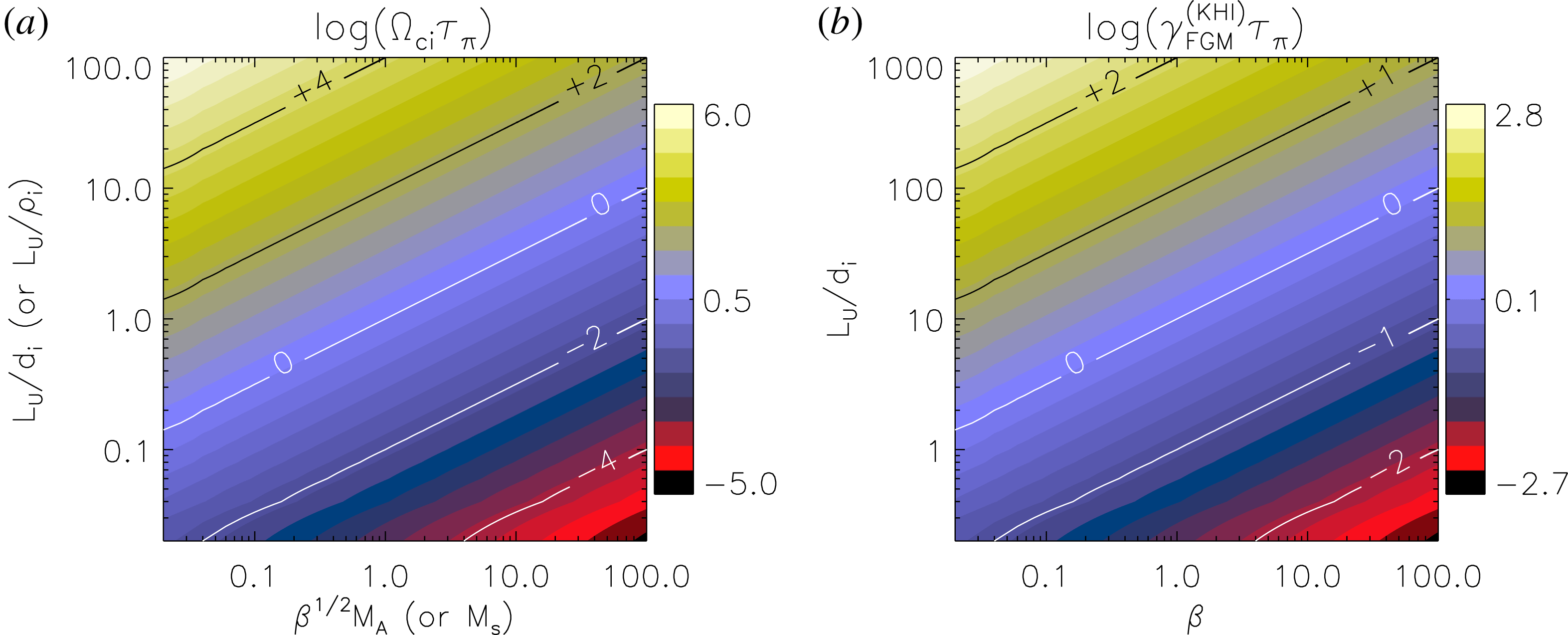
A sketch of the behaviour of time scales in (2.16) and (2.18) with respect to the relevant parameters is provided in figure 1. MHD-like behaviour is recovered in the parameter space denoted by yellow/white colours.
2.4 Sustainability of pressure agyrotropy
An interesting feature of the interaction between the pressure tensor and a sheared flow is the sustainability and/or the generation of pressure ‘agyrotropy’ (Cerri et al.
Reference Cerri, Henri, Califano, Del Sarto, Faganello and Pegoraro2013, Reference Cerri, Pegoraro, Califano, Del Sarto and Jenko2014; Del Sarto et al.
Reference Del Sarto, Pegoraro and Califano2016, Reference Del Sarto, Pegoraro and Tenerani2017). This means that, in addition to the typical pressure anisotropy with respect to the magnetic-field direction that is typical of collisionless plasmas ( $p_{\bot }\neq p_{\Vert }$
), now additional pressure anisotropy can be present in the plane perpendicular to
$p_{\bot }\neq p_{\Vert }$
), now additional pressure anisotropy can be present in the plane perpendicular to $\boldsymbol{B}$
, e.g.
$\boldsymbol{B}$
, e.g. $p_{\bot ,1}\neq p_{\bot ,2}\neq p_{\Vert }$
, where (
$p_{\bot ,1}\neq p_{\bot ,2}\neq p_{\Vert }$
, where ( $\boldsymbol{e}_{\bot ,1}$
,
$\boldsymbol{e}_{\bot ,1}$
, $\boldsymbol{e}_{\bot ,2}$
,
$\boldsymbol{e}_{\bot ,2}$
, $\boldsymbol{e}_{\Vert }$
) is any orthogonal basis within which the pressure tensor is diagonal and where
$\boldsymbol{e}_{\Vert }$
) is any orthogonal basis within which the pressure tensor is diagonal and where $\boldsymbol{e}_{\bot ,1}$
and
$\boldsymbol{e}_{\bot ,1}$
and $\boldsymbol{e}_{\bot ,2}$
define the plane perpendicular to the magnetic field. In this section we analyse this aspect in terms of equilibrium configurations and their corresponding agyrotropy. However, we stress that this feature has consequences for the dynamics of a collisionless plasma as well, e.g. modifying linear properties of perturbations (e.g. Del Sarto et al.
Reference Del Sarto, Pegoraro and Califano2016, Reference Del Sarto, Pegoraro and Tenerani2017), enhancing the kinetic activity related to vorticity, current sheets, reconnection and energy transfer in turbulence (e.g. Greco et al.
Reference Greco, Valentini, Servidio and Matthaeus2012; Servidio et al.
Reference Servidio, Valentini, Califano and Veltri2012, Reference Servidio, Osman, Valentini, Perrone, Califano, Chapman, Matthaeus and Veltri2014; Yang et al.
Reference Yang, Matthaeus, Parashar, Haggerty, Roytershteyn, Daughton, Wan, Shi and Chen2017) and possibly affecting the regulation of anisotropies in accretion disks (e.g. Kunz, Stone & Quataert Reference Kunz, Stone and Quataert2016).
$\boldsymbol{e}_{\bot ,2}$
define the plane perpendicular to the magnetic field. In this section we analyse this aspect in terms of equilibrium configurations and their corresponding agyrotropy. However, we stress that this feature has consequences for the dynamics of a collisionless plasma as well, e.g. modifying linear properties of perturbations (e.g. Del Sarto et al.
Reference Del Sarto, Pegoraro and Califano2016, Reference Del Sarto, Pegoraro and Tenerani2017), enhancing the kinetic activity related to vorticity, current sheets, reconnection and energy transfer in turbulence (e.g. Greco et al.
Reference Greco, Valentini, Servidio and Matthaeus2012; Servidio et al.
Reference Servidio, Valentini, Califano and Veltri2012, Reference Servidio, Osman, Valentini, Perrone, Califano, Chapman, Matthaeus and Veltri2014; Yang et al.
Reference Yang, Matthaeus, Parashar, Haggerty, Roytershteyn, Daughton, Wan, Shi and Chen2017) and possibly affecting the regulation of anisotropies in accretion disks (e.g. Kunz, Stone & Quataert Reference Kunz, Stone and Quataert2016).
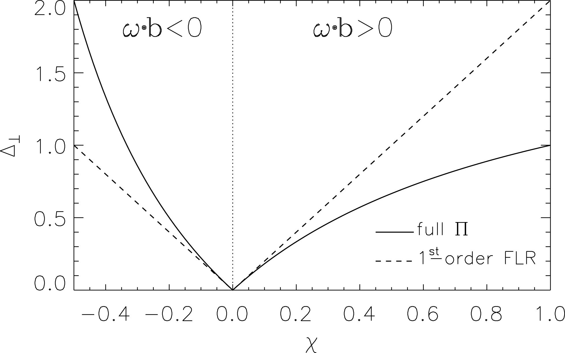
Pressure anisotropy in the plane perpendicular to the magnetic field direction, $\unicode[STIX]{x1D6E5}_{\bot }$
, versus
$\unicode[STIX]{x1D6E5}_{\bot }$
, versus $\unicode[STIX]{x1D712}\equiv \unicode[STIX]{x1D74E}\boldsymbol{\cdot }\boldsymbol{b}/2\unicode[STIX]{x1D6FA}_{c\text{i}}$
obtained from first-order FLR corrections (dashed line, equation (2.19)) and from the full pressure-tensor equation (continuous line, equation (2.20)). Positivity of pressure from the full-
$\unicode[STIX]{x1D712}\equiv \unicode[STIX]{x1D74E}\boldsymbol{\cdot }\boldsymbol{b}/2\unicode[STIX]{x1D6FA}_{c\text{i}}$
obtained from first-order FLR corrections (dashed line, equation (2.19)) and from the full pressure-tensor equation (continuous line, equation (2.20)). Positivity of pressure from the full- $\unicode[STIX]{x1D6F1}$
treatment requires
$\unicode[STIX]{x1D6F1}$
treatment requires $\unicode[STIX]{x1D712}\geqslant -1/2$
(see Cerri et al.
Reference Cerri, Pegoraro, Califano, Del Sarto and Jenko2014), while the FLR treatment holds for
$\unicode[STIX]{x1D712}\geqslant -1/2$
(see Cerri et al.
Reference Cerri, Pegoraro, Califano, Del Sarto and Jenko2014), while the FLR treatment holds for $|\unicode[STIX]{x1D712}|\ll 1$
.
$|\unicode[STIX]{x1D712}|\ll 1$
.
In our configuration it is easy to show that the FLR effects introduce an agyrotropy, $\unicode[STIX]{x1D6E5}_{\bot }$
, i.e. an anisotropy in the plane perpendicular to the magnetic field (see, e.g. Scudder & Daughton Reference Scudder and Daughton2008, for a general formulation), given by
$\unicode[STIX]{x1D6E5}_{\bot }$
, i.e. an anisotropy in the plane perpendicular to the magnetic field (see, e.g. Scudder & Daughton Reference Scudder and Daughton2008, for a general formulation), given by
 $$\begin{eqnarray}\unicode[STIX]{x1D6E5}_{\bot }=\frac{|\unicode[STIX]{x1D74E}\boldsymbol{\cdot }\boldsymbol{b}|}{\unicode[STIX]{x1D6FA}_{ci}}\equiv |2\unicode[STIX]{x1D712}|.\end{eqnarray}$$
Since only the first-order FLR corrections have been retained in the present description, only small deviations from gyrotropy are correctly described in this case, i.e. the condition $|\unicode[STIX]{x1D712}|=|\unicode[STIX]{x1D74E}\boldsymbol{\cdot }\boldsymbol{b}/2\unicode[STIX]{x1D6FA}_{c\text{i}}|\ll 1$
should hold. Also, in this approximation the equilibrium exhibits an asymmetry with respect to the sign of
$|\unicode[STIX]{x1D712}|=|\unicode[STIX]{x1D74E}\boldsymbol{\cdot }\boldsymbol{b}/2\unicode[STIX]{x1D6FA}_{c\text{i}}|\ll 1$
should hold. Also, in this approximation the equilibrium exhibits an asymmetry with respect to the sign of $\unicode[STIX]{x1D74E}\boldsymbol{\cdot }\boldsymbol{b}$
, but
$\unicode[STIX]{x1D74E}\boldsymbol{\cdot }\boldsymbol{b}$
, but $\unicode[STIX]{x1D6E5}_{\bot }$
does not. In order to have such asymmetry in the agyrotropy, next-order corrections or the full pressure tensor must be retained. In the latter case, the agyrotropy in the plane perpendicular to
$\unicode[STIX]{x1D6E5}_{\bot }$
does not. In order to have such asymmetry in the agyrotropy, next-order corrections or the full pressure tensor must be retained. In the latter case, the agyrotropy in the plane perpendicular to $\boldsymbol{B}$
would be (Cerri et al.
Reference Cerri, Pegoraro, Califano, Del Sarto and Jenko2014)
$\boldsymbol{B}$
would be (Cerri et al.
Reference Cerri, Pegoraro, Califano, Del Sarto and Jenko2014)
 $$\begin{eqnarray}\unicode[STIX]{x1D6E5}_{\bot }=\left|\frac{2\unicode[STIX]{x1D712}}{1+\unicode[STIX]{x1D712}}\right|,\end{eqnarray}$$
where the condition $\unicode[STIX]{x1D712}\geqslant -1/2$
must hold because of the positivity constraint on pressure.
$\unicode[STIX]{x1D712}\geqslant -1/2$
must hold because of the positivity constraint on pressure.
In figure 2 we report a comparison between the pressure anisotropy in the plane perpendicular to the magnetic field, $\unicode[STIX]{x1D6E5}_{\bot }$
, as a function of the parameter
$\unicode[STIX]{x1D6E5}_{\bot }$
, as a function of the parameter $\unicode[STIX]{x1D712}$
, obtained via the full pressure-tensor equation (Cerri et al.
Reference Cerri, Pegoraro, Califano, Del Sarto and Jenko2014) and via first-order FLR corrections.
$\unicode[STIX]{x1D712}$
, obtained via the full pressure-tensor equation (Cerri et al.
Reference Cerri, Pegoraro, Califano, Del Sarto and Jenko2014) and via first-order FLR corrections.
2.5 A broader view: relevance to other instabilities and turbulent environments
As we will show in § 3, the main consequences related to the ion-FLR effects reported in this paper have a direct effect in the current system of a planetary magnetopause. Moreover, these ion-kinetic effects can cause the asymmetric development of KHI at the dawn and the dusk sides of such magnetosphere, as well as other non-ideal features (see, e.g. Nagano Reference Nagano1978; Huba Reference Huba1996; Terada et al. Reference Terada, Machida and Shinagawa2002; Nakamura et al. Reference Nakamura, Hasegawa and Shinohara2010; Henri et al. Reference Henri, Califano, Faganello and Pegoraro2012; Masters et al. Reference Masters, Achilleos, Cutler, Coates, Dougherty and Jones2012; Sundberg et al. Reference Sundberg, Boardsen, Slavin, Anderson, Korth, Zurbuchen, Raines and Solomon2012; Taylor et al. Reference Taylor, Hasegawa, Lavraud, Phan, Escoubet, Dunlop, Bogdanova, Borg, Volwerk and Berchem2012; Delamere et al. Reference Delamere, Wilson, Eriksson and Bagenal2013; Paral & Rankin Reference Paral and Rankin2013; Haaland et al. Reference Haaland, Reistad, Tenfjord, Gjerloev, Maes, Dekeyser, Maggiolo, Anekallu and Dorville2014; Johnson et al. Reference Johnson, Wing and Delamere2014; Liljeblad et al. Reference Liljeblad, Sundberg, Karlsson and Kullen2014; Walsh et al. Reference Walsh, Haaland, Forsyth, Keesee, Kissinger, Li, Runov, Soucek, Walsh and Wing2014; Gershman et al. Reference Gershman, Raines, Slavin, Zurbuchen, Sundberg, Boardsen, Anderson, Korth and Solomon2015; Gingell et al. Reference Gingell, Sundberg and Burgess2015; De Camillis et al. Reference De Camillis, Cerri, Califano and Pegoraro2016). However, ion-FLR effects and their relations with anisotropy, vorticity and current sheets can have implications on a wide variety of astrophysical and space scenarios.
In fact there are further shear-driven instabilities that may also get relevant feedback from anisotropy (and agyrotropy) developed (or sustained) by the underlying shear flow within a kinetic description such as, for instance, for the case of magneto-rotational instability (MRI) in accretion disks (e.g. Ferraro Reference Ferraro2007; Riquelme et al. Reference Riquelme, Quataert, Sharma and Spitkovsky2012; Kunz et al. Reference Kunz, Stone and Quataert2016; Squire, Quataert & Kunz Reference Squire, Quataert and Kunz2017b ). Furthermore, ion-kinetic effects such as FLR and pressure-tensor dynamics can affect anisotropy-driven instabilities themselves (e.g. Schekochihin et al. Reference Schekochihin, Cowley, Rincon and Rosin2010; Rosin et al. Reference Rosin, Schekochihin, Rincon and Cowley2011; Sarrat, Del Sarto & Ghizzo Reference Sarrat, Del Sarto and Ghizzo2016; Squire et al. Reference Squire, Kunz, Quataert and Schekochihin2017a ), which are relevant, e.g. in the evolution of the solar wind (e.g. Hellinger et al. Reference Hellinger, Trávníček, Kasper and Lazarus2006; Tenerani, Velli & Hellinger Reference Tenerani, Velli and Hellinger2017; Yoon Reference Yoon2017) and in magnetic reconnection (e.g. Schoeffler, Drake & Swisdak Reference Schoeffler, Drake and Swisdak2011; Cassak et al. Reference Cassak, Baylor, Fermo, Beidler, Shay, Swisdak, Drake and Karimabadi2015).
Finally, current sheets and the associated reconnection processes are fundamental ingredients of turbulent plasmas (e.g. Matthaeus & Lamkin Reference Matthaeus and Lamkin1986; Biskamp Reference Biskamp2008; Servidio et al. Reference Servidio, Matthaeus, Shay, Dmitruk, Cassak and Wan2010, Reference Servidio, Dmitruk, Greco, Wan, Donato, Cassak, Shay, Carbone and Matthaeus2011; Lazarian, Eyink & Vishniac Reference Lazarian, Eyink and Vishniac2012; Karimabadi et al. Reference Karimabadi, Roytershteyn, Daughton and Liu2013a ; Servidio et al. Reference Servidio, Valentini, Perrone, Greco, Califano, Matthaeus and Veltri2015; Franci et al. Reference Franci, Hellinger, Matteini, Verdini and Landi2016; Cerri et al. Reference Cerri, Franci, Califano, Landi and Hellinger2017). In this context, currents and coherent structures are typically related to simultaneous enhancement of vorticity, kinetic activity, turbulent transfer and dissipation (e.g. Servidio et al. Reference Servidio, Valentini, Califano and Veltri2012, Reference Servidio, Osman, Valentini, Perrone, Califano, Chapman, Matthaeus and Veltri2014; Karimabadi et al. Reference Karimabadi, Roytershteyn, Wan, Matthaeus, Daughton, Wu, Shay, Loring, Borovsky and Leonardis2013b ; Valentini et al. Reference Valentini, Servidio, Perrone, Califano, Matthaeus and Veltri2014, Reference Valentini, Perrone, Stabile, Pezzi, Servidio, De Marco, Marcucci, Bruno, Lavraud and De Keyser2016; Wan et al. Reference Wan, Matthaeus, Roytershteyn, Karimabadi, Parashar, Wu and Shay2015; Franci et al. Reference Franci, Hellinger, Matteini, Verdini and Landi2016; Parashar & Matthaeus Reference Parashar and Matthaeus2016; Yang et al. Reference Yang, Matthaeus, Parashar, Haggerty, Roytershteyn, Daughton, Wan, Shi and Chen2017; Grošelj et al. Reference Grošelj, Cerri, Bañón Navarro, Willmott, Told, Loureiro, Califano and Jenko2017; Camporeale et al. Reference Camporeale, Sorriso-Valvo, Califano and Retinò2018; Sorriso-Valvo et al. Reference Sorriso-Valvo, Perrone, Pezzi, Valentini, Servidio, Zouganelis and Veltri2018). Furthermore, reconnection/structures have been recently proved to enhance/trigger the kinetic turbulent cascades in real space (Cerri & Califano Reference Cerri and Califano2017; Franci et al. Reference Franci, Cerri, Califano, Landi, Papini, Verdini, Matteini, Jenko and Hellinger2017; Camporeale et al. Reference Camporeale, Sorriso-Valvo, Califano and Retinò2018) and also to be related to simultaneous velocity-space cascades (Servidio et al. Reference Servidio, Chasapis, Matthaeus, Perrone, Valentini, Parashar, Veltri, Gershman, Russell and Giles2017; Cerri, Kunz & Califano Reference Cerri, Kunz and Califano2018; Pezzi et al. Reference Pezzi, Servidio, Perrone, Valentini, Sorriso-Valvo, Greco, Matthaeus and Veltri2018). These reconnecting current sheets and the resulting magnetic structures are quasi-equilibrium pressure-balanced structures with embedded sheared flows even within a turbulent environment (see e.g. Cerri & Califano Reference Cerri and Califano2017). Therefore ion-kinetic effects such as FLR contributions (or the full pressure tensor; see Cerri et al. (Reference Cerri, Pegoraro, Califano, Del Sarto and Jenko2014), Yang et al. (Reference Yang, Matthaeus, Parashar, Haggerty, Roytershteyn, Daughton, Wan, Shi and Chen2017) and Del Sarto & Pegoraro (Reference Del Sarto and Pegoraro2018)) may play a relevant role in the complex interplay between currents, vorticity, reconnection, non-Maxwellian features, velocity-space cascades and dissipation in turbulent plasmas.
3 Application to the LLBL of the Earth’s magnetopause
Let us now consider an explicit application to the LLBL of the Earth’s magnetopause, the goal being to show that the observed deviations from the ideal Chapman–Ferraro current system highlighted in Haaland et al. (Reference Haaland, Reistad, Tenfjord, Gjerloev, Maes, Dekeyser, Maggiolo, Anekallu and Dorville2014) can be qualitatively explained with the ion-FLR corrections. We want to stress that this is not meant to be a quantitative explanation of the observed profiles, since also the three-dimensional geometry and other effects may contribute to the actual profiles. In what follows, equations are normalized to the proton mass, inertial length and cyclotron frequency ( $m_{\text{p}}$
,
$m_{\text{p}}$
, $d_{\text{p}}$
and
$d_{\text{p}}$
and $\unicode[STIX]{x1D6FA}_{c\text{p}}$
, respectively), and the Alfvén speed (
$\unicode[STIX]{x1D6FA}_{c\text{p}}$
, respectively), and the Alfvén speed ( $v_{A}$
).
$v_{A}$
).
We consider a local one-dimensional model the LLBL region in which the inhomogeneity direction ( $x$
) is perpendicular to the plane (
$x$
) is perpendicular to the plane ( $yz$
) where both the flow and the magnetic field lie. Typically, hyperbolic tangent give a reasonably realistic modelling of the flow,
$yz$
) where both the flow and the magnetic field lie. Typically, hyperbolic tangent give a reasonably realistic modelling of the flow,
 $$\begin{eqnarray}\displaystyle & \displaystyle u_{y}(x)=u_{0}\sin \unicode[STIX]{x1D719}\tanh \left(\frac{x-x_{u,0}}{L_{u}}\right), & \displaystyle\end{eqnarray}$$
 $$\begin{eqnarray}\displaystyle & \displaystyle u_{z}(x)=u_{0}\cos \unicode[STIX]{x1D719}\tanh \left(\frac{x-x_{u,0}}{L_{u}}\right), & \displaystyle\end{eqnarray}$$
where $\unicode[STIX]{x1D719}$
is the angle between the
$\unicode[STIX]{x1D719}$
is the angle between the $z$
-axis and the plane where the sheared flow velocity lies, and of the magnetic field,
$z$
-axis and the plane where the sheared flow velocity lies, and of the magnetic field,
 $$\begin{eqnarray}\displaystyle B_{y}(x) & = & \displaystyle B_{0}\left\{\frac{B_{G}}{B_{0}}\sin \unicode[STIX]{x1D717}\left[1+\frac{\unicode[STIX]{x0394}B_{\Vert }}{2B_{G}}\left(1-\tanh \left(\frac{x-x_{B,0}}{L_{B}}\right)\right)\right]\right.\nonumber\\ \displaystyle & & \displaystyle +\left.\frac{\unicode[STIX]{x0394}B_{\bot }}{2B_{0}}\cos \unicode[STIX]{x1D717}\left[1+\tanh \left(\frac{x-x_{B,0}}{L_{B}}\right)\right]\!\right\},\end{eqnarray}$$
 $$\begin{eqnarray}\displaystyle B_{z}(x) & = & \displaystyle B_{0}\left\{\frac{B_{G}}{B_{0}}\cos \unicode[STIX]{x1D717}\left[1+\frac{\unicode[STIX]{x0394}B_{\Vert }}{2B_{G}}\left(1-\tanh \left(\frac{x-x_{B,0}}{L_{B}}\right)\right)\right]\right.\nonumber\\ \displaystyle & & \displaystyle -\left.\frac{\unicode[STIX]{x0394}B_{\bot }}{2B_{0}}\sin \unicode[STIX]{x1D717}\left[1+\tanh \left(\frac{x-x_{B,0}}{L_{B}}\right)\right]\!\right\},\end{eqnarray}$$
where $B_{0}=\sqrt{B_{G}^{2}+\unicode[STIX]{x0394}B_{\bot }^{2}}$
and
$B_{0}=\sqrt{B_{G}^{2}+\unicode[STIX]{x0394}B_{\bot }^{2}}$
and $\unicode[STIX]{x1D717}$
is the angle between the
$\unicode[STIX]{x1D717}$
is the angle between the $z$
-axis and the magnetic field at
$z$
-axis and the magnetic field at $x\rightarrow -\infty$
Footnote
5
. The above magnetic profile accounts both for variations that are purely in magnitude, through
$x\rightarrow -\infty$
Footnote
5
. The above magnetic profile accounts both for variations that are purely in magnitude, through $\unicode[STIX]{x0394}B_{\Vert }$
, and for rotations (magnetic shear) of the magnetic-field direction, through
$\unicode[STIX]{x0394}B_{\Vert }$
, and for rotations (magnetic shear) of the magnetic-field direction, through $\unicode[STIX]{x0394}B_{\bot }$
(see, e.g. Fadanelli et al.
Reference Fadanelli, Faganello, Califano, Cerri, Pegoraro and Lavraud2018, for the effects of
$\unicode[STIX]{x0394}B_{\bot }$
(see, e.g. Fadanelli et al.
Reference Fadanelli, Faganello, Califano, Cerri, Pegoraro and Lavraud2018, for the effects of $\unicode[STIX]{x0394}B_{\bot }$
on KHI at the Earth’s magnetospheric flanks). Note that usually
$\unicode[STIX]{x0394}B_{\bot }$
on KHI at the Earth’s magnetospheric flanks). Note that usually $x_{u,0}=x_{B,0}$
and
$x_{u,0}=x_{B,0}$
and $L_{u}=L_{B}$
are assumed in numerical simulations (see, e.g. Miura Reference Miura1987; Fujimoto & Terasawa Reference Fujimoto and Terasawa1995; Otto & Fairfield Reference Otto and Fairfield2000; Nykyri & Otto Reference Nykyri and Otto2004; Nakamura & Fujimoto Reference Nakamura and Fujimoto2005; Faganello, Califano & Pegoraro Reference Faganello, Califano and Pegoraro2008; Palermo et al.
Reference Palermo, Faganello, Califano, Pegoraro and Le Contel2011; Tenerani et al.
Reference Tenerani, Faganello, Califano and Pegoraro2011; Faganello et al.
Reference Faganello, Califano, Pegoraro and Andreussi2012). However, recent satellite measurements have shown that the magnetic (and density) profiles can be slightly shifted with respect to the velocity shear and/or that the shear length scales of these quantities may differ, i.e.
$L_{u}=L_{B}$
are assumed in numerical simulations (see, e.g. Miura Reference Miura1987; Fujimoto & Terasawa Reference Fujimoto and Terasawa1995; Otto & Fairfield Reference Otto and Fairfield2000; Nykyri & Otto Reference Nykyri and Otto2004; Nakamura & Fujimoto Reference Nakamura and Fujimoto2005; Faganello, Califano & Pegoraro Reference Faganello, Califano and Pegoraro2008; Palermo et al.
Reference Palermo, Faganello, Califano, Pegoraro and Le Contel2011; Tenerani et al.
Reference Tenerani, Faganello, Califano and Pegoraro2011; Faganello et al.
Reference Faganello, Califano, Pegoraro and Andreussi2012). However, recent satellite measurements have shown that the magnetic (and density) profiles can be slightly shifted with respect to the velocity shear and/or that the shear length scales of these quantities may differ, i.e. $x_{u,0}\neq x_{n,0}$
and/or
$x_{u,0}\neq x_{n,0}$
and/or $L_{u}\neq L_{n}$
(Foullon et al.
Reference Foullon, Farrugia, Fazakerley, Owen, Gratton and Torbert2008; Haaland et al.
Reference Haaland, Reistad, Tenfjord, Gjerloev, Maes, Dekeyser, Maggiolo, Anekallu and Dorville2014; Rossi Reference Rossi2015). This idea has been also recently implemented in numerical simulations in order to explain some observational features (Rossi Reference Rossi2015; Leroy & Keppens Reference Leroy and Keppens2017). Therefore, here we also take into account these features. For a magnetic profile as in (3.3)–(3.4) the MHD magnetic pressure function,
$L_{u}\neq L_{n}$
(Foullon et al.
Reference Foullon, Farrugia, Fazakerley, Owen, Gratton and Torbert2008; Haaland et al.
Reference Haaland, Reistad, Tenfjord, Gjerloev, Maes, Dekeyser, Maggiolo, Anekallu and Dorville2014; Rossi Reference Rossi2015). This idea has been also recently implemented in numerical simulations in order to explain some observational features (Rossi Reference Rossi2015; Leroy & Keppens Reference Leroy and Keppens2017). Therefore, here we also take into account these features. For a magnetic profile as in (3.3)–(3.4) the MHD magnetic pressure function, ${\mathcal{H}}$
, is given by
${\mathcal{H}}$
, is given by
 $$\begin{eqnarray}\displaystyle {\mathcal{H}}(x)=\frac{B_{G}^{2}}{B_{0}^{2}}\left\{\!\left[1+\frac{\unicode[STIX]{x0394}B_{\Vert }}{2B_{G}}\left(1-\tanh \left(\frac{x-x_{B,0}}{L_{B}}\right)\right)\right]^{2}+\frac{\unicode[STIX]{x0394}B_{\bot }^{2}}{4B_{G}^{2}}\left[1+\tanh \left(\frac{x-x_{B,0}}{L_{B}}\right)\right]^{2}\right\},\hspace{-9.60004pt} & & \displaystyle \nonumber\\ \displaystyle & & \displaystyle\end{eqnarray}$$
and the corresponding MHD thermal profiles are obtained in terms of
 $$\begin{eqnarray}\displaystyle {\mathcal{F}}_{\bot }(x)={\mathcal{G}}_{\bot }(x) & = & \displaystyle 1+\frac{\unicode[STIX]{x0394}B_{\bot }^{2}}{\unicode[STIX]{x1D6FD}_{\bot ,0}B_{0}^{2}}-\frac{B_{G}\unicode[STIX]{x0394}B_{\Vert }}{\unicode[STIX]{x1D6FD}_{\bot ,0}B_{0}^{2}}\left[1-\tanh \left(\frac{x-x_{B,0}}{L_{B}}\right)\right]\nonumber\\ \displaystyle & & \displaystyle -\,\frac{\unicode[STIX]{x0394}B_{\Vert }^{2}}{4\unicode[STIX]{x1D6FD}_{\bot ,0}B_{0}^{2}}\left[1-\tanh \left(\frac{x-x_{B,0}}{L_{B}}\right)\right]^{2}\nonumber\\ \displaystyle & & \displaystyle -\,\frac{\unicode[STIX]{x0394}B_{\bot }^{2}}{4\unicode[STIX]{x1D6FD}_{\bot ,0}B_{0}^{2}}\left[1+\tanh \left(\frac{x-x_{B,0}}{L_{B}}\right)\right]^{2},\end{eqnarray}$$
where $\unicode[STIX]{x1D6FD}_{\bot ,0}B_{0}^{2}=2P_{\bot ,0}\equiv 2(p_{\bot \text{p},0}+p_{\bot \text{e},0})$
and the positivity condition on pressure (see (A 10) in § A.3) here reads as
$\unicode[STIX]{x1D6FD}_{\bot ,0}B_{0}^{2}=2P_{\bot ,0}\equiv 2(p_{\bot \text{p},0}+p_{\bot \text{e},0})$
and the positivity condition on pressure (see (A 10) in § A.3) here reads as
 $$\begin{eqnarray}B_{G}\unicode[STIX]{x0394}B_{\Vert }+\frac{\unicode[STIX]{x0394}B_{\Vert }^{2}}{2}\leqslant P_{\bot ,0}+\frac{\unicode[STIX]{x0394}B_{\bot }^{2}}{2}.\end{eqnarray}$$
The FLR corrections to the above MHD profiles are then given in terms of
 $$\begin{eqnarray}\displaystyle \widetilde{U}^{\prime }(x) & = & \displaystyle \frac{\widetilde{\unicode[STIX]{x1D6FD}}_{\bot \text{p},0}}{2}\frac{u_{0}}{B_{0}L_{u}}\frac{{\mathcal{F}}_{\bot }(x)}{{\mathcal{H}}(x)}\cosh ^{-2}\left(\frac{x-x_{u,0}}{L_{u}}\right)\nonumber\\ \displaystyle & & \displaystyle \times \,\left\{\frac{B_{G}}{B_{0}}\left[1+\frac{\unicode[STIX]{x0394}B_{\Vert }}{2B_{G}}\left(1-\tanh \left(\frac{x-x_{B,0}}{L_{B}}\right)\right)\right]\sin (\unicode[STIX]{x1D719}-\unicode[STIX]{x1D717})\right.\nonumber\\ \displaystyle & & \displaystyle -\left.\frac{\unicode[STIX]{x0394}B_{\bot }}{2B_{0}}\left[1+\tanh \left(\frac{x-x_{B,0}}{L_{B}}\right)\right]\cos (\unicode[STIX]{x1D719}-\unicode[STIX]{x1D717})\right\},\end{eqnarray}$$
which is again related to the sign of the scalar product between the fluid vorticity and the magnetic field through the $\sin (\unicode[STIX]{x1D719}-\unicode[STIX]{x1D717})$
and
$\sin (\unicode[STIX]{x1D719}-\unicode[STIX]{x1D717})$
and $\cos (\unicode[STIX]{x1D719}-\unicode[STIX]{x1D717})$
coefficients.
$\cos (\unicode[STIX]{x1D719}-\unicode[STIX]{x1D717})$
coefficients.
3.1 Current profiles at the Earth’s flank magnetopause: an example
Let us now consider a few explicit examples relevant for the magnetopause layer and see how the first-order FLR corrections qualitatively modify its current profile. For the sake of simplicity, we consider the case of $\unicode[STIX]{x1D717}=0$
and
$\unicode[STIX]{x1D717}=0$
and $\unicode[STIX]{x1D719}=\unicode[STIX]{x03C0}/2$
and two slightly different regimes are taken into account. A summary of the parameters adopted for the example profiles is given in table 1. These parameters are chosen so that they are as realistic as possible for the low-latitude flanks of the magnetopause (Haaland et al.
Reference Haaland, Reistad, Tenfjord, Gjerloev, Maes, Dekeyser, Maggiolo, Anekallu and Dorville2014), and they are also able to somewhat emphasize some of the resulting features Footnote
6
.
$\unicode[STIX]{x1D719}=\unicode[STIX]{x03C0}/2$
and two slightly different regimes are taken into account. A summary of the parameters adopted for the example profiles is given in table 1. These parameters are chosen so that they are as realistic as possible for the low-latitude flanks of the magnetopause (Haaland et al.
Reference Haaland, Reistad, Tenfjord, Gjerloev, Maes, Dekeyser, Maggiolo, Anekallu and Dorville2014), and they are also able to somewhat emphasize some of the resulting features Footnote
6
.
Summary of the parameters used for profiles in figure 3. All the parameters are normalized with respect to quantities characteristic of the SW region: flow speed is in $v_{\text{A}}^{\text{(SW)}}$
units, lengths are in
$v_{\text{A}}^{\text{(SW)}}$
units, lengths are in $d_{\text{i}}^{\text{(SW)}}$
units and magnetic-field variations are in
$d_{\text{i}}^{\text{(SW)}}$
units and magnetic-field variations are in $B_{0}^{\text{(SW)}}=1$
units (from which
$B_{0}^{\text{(SW)}}=1$
units (from which $B_{G}=\sqrt{1-\unicode[STIX]{x0394}B_{\bot }^{2}}$
follows). The plus and minus sign in
$B_{G}=\sqrt{1-\unicode[STIX]{x0394}B_{\bot }^{2}}$
follows). The plus and minus sign in $u_{0}$
and in
$u_{0}$
and in $x_{u,0}$
are for the dusk and for the dawn side, respectively. We also remind the reader that
$x_{u,0}$
are for the dusk and for the dawn side, respectively. We also remind the reader that $\unicode[STIX]{x1D717}=0$
and
$\unicode[STIX]{x1D717}=0$
and $\unicode[STIX]{x1D719}=\unicode[STIX]{x03C0}/2$
in both cases.
$\unicode[STIX]{x1D719}=\unicode[STIX]{x03C0}/2$
in both cases.

Current profiles for cases reported in table 1. (a,b) Case A, dawn (a) and dusk (b) sides. (c,d) Case B, dawn (c) and dusk (d) sides. The MHD current profiles, $J_{y}^{\text{(MHD)}}$
and
$J_{y}^{\text{(MHD)}}$
and $J_{z}^{\text{(MHD)}}$
, are reported with dashed light blue and dot-dashed orange lines, respectively, whereas the corresponding FLR-corrected profiles,
$J_{z}^{\text{(MHD)}}$
, are reported with dashed light blue and dot-dashed orange lines, respectively, whereas the corresponding FLR-corrected profiles, $J_{y}^{\text{(FLR)}}$
and
$J_{y}^{\text{(FLR)}}$
and $J_{z}^{\text{(FLR)}}$
, are drawn in blue and red solid lines, respectively.
$J_{z}^{\text{(FLR)}}$
, are drawn in blue and red solid lines, respectively.

In figure 3 we report the current profile arising from a simple MHD configuration, $J_{y}^{\text{(MHD)}}$
and
$J_{y}^{\text{(MHD)}}$
and $J_{z}^{\text{(MHD)}}$
(light blue dashed line and orange dot-dashed line, respectively), as well as the profile accounting for the first-order FLR corrections in (3.8),
$J_{z}^{\text{(MHD)}}$
(light blue dashed line and orange dot-dashed line, respectively), as well as the profile accounting for the first-order FLR corrections in (3.8), $J_{y}^{\text{(FLR)}}$
and
$J_{y}^{\text{(FLR)}}$
and $J_{z}^{\text{(FLR)}}$
(blue and red solid lines, respectively). The MHD profiles of the dusk and of the dawn sides, apart from the sign, have the same shape, i.e. it is the classic Chapman–Ferraro current layer (Chapman & Ferraro Reference Chapman and Ferraro1930). On the other hand, the corresponding FLR-corrected profiles of the dawn and of the dusk sides are qualitatively different. This is the effect of the ‘
$J_{z}^{\text{(FLR)}}$
(blue and red solid lines, respectively). The MHD profiles of the dusk and of the dawn sides, apart from the sign, have the same shape, i.e. it is the classic Chapman–Ferraro current layer (Chapman & Ferraro Reference Chapman and Ferraro1930). On the other hand, the corresponding FLR-corrected profiles of the dawn and of the dusk sides are qualitatively different. This is the effect of the ‘ $\unicode[STIX]{x1D74E}\boldsymbol{b}$
asymmetry’ intrinsically encoded in the FLR contributions. Furthermore, the current structure of the shear layer in this latter case is much more complex than the Chapman–Ferraro MHD layer. In fact, a double-peak feature asymmetrically arises in
$\unicode[STIX]{x1D74E}\boldsymbol{b}$
asymmetry’ intrinsically encoded in the FLR contributions. Furthermore, the current structure of the shear layer in this latter case is much more complex than the Chapman–Ferraro MHD layer. In fact, a double-peak feature asymmetrically arises in $J^{\text{(FLR)}}$
on the two sides of the flank magnetopause and the different modification of the two components of the current results in adjacent current sheets with different current directions (see figure 4, where we report the
$J^{\text{(FLR)}}$
on the two sides of the flank magnetopause and the different modification of the two components of the current results in adjacent current sheets with different current directions (see figure 4, where we report the $x$
-dependence of the angle between
$x$
-dependence of the angle between $\boldsymbol{J}$
and the
$\boldsymbol{J}$
and the $z$
-axis,
$z$
-axis, $\unicode[STIX]{x1D6FC}=\arctan (J_{y}/J_{z})$
, for the cases shown in figure 3). These three peculiar features, namely (i) the dusk–dawn asymmetry of the current layer, (ii) the double-peak feature in the current profiles and (iii) two (or more) adjacent current sheets having thickness of several ion Larmor radii and with different current directions, are qualitatively consistent with the Cluster observations reported in Haaland et al. (Reference Haaland, Reistad, Tenfjord, Gjerloev, Maes, Dekeyser, Maggiolo, Anekallu and Dorville2014). Taking into account these FLR effects can also be a relevant starting point for explaining certain anomalies occurring during magnetopause distortions related to large-scale magnetosheath plasma jets (see, e.g. Dmitriev & Suvorova Reference Dmitriev and Suvorova2012).
$\unicode[STIX]{x1D6FC}=\arctan (J_{y}/J_{z})$
, for the cases shown in figure 3). These three peculiar features, namely (i) the dusk–dawn asymmetry of the current layer, (ii) the double-peak feature in the current profiles and (iii) two (or more) adjacent current sheets having thickness of several ion Larmor radii and with different current directions, are qualitatively consistent with the Cluster observations reported in Haaland et al. (Reference Haaland, Reistad, Tenfjord, Gjerloev, Maes, Dekeyser, Maggiolo, Anekallu and Dorville2014). Taking into account these FLR effects can also be a relevant starting point for explaining certain anomalies occurring during magnetopause distortions related to large-scale magnetosheath plasma jets (see, e.g. Dmitriev & Suvorova Reference Dmitriev and Suvorova2012).
Profiles of the angle between the current $\boldsymbol{J}$
and the
$\boldsymbol{J}$
and the $z$
-axis,
$z$
-axis, $\unicode[STIX]{x1D6FC}$
, versus
$\unicode[STIX]{x1D6FC}$
, versus $x$
for cases reported in figure 3. (a) Case A, dawn (a,b) and dusk (b) sides. (c,d) Case B, dawn (c) and dusk (d) sides.
$x$
for cases reported in figure 3. (a) Case A, dawn (a,b) and dusk (b) sides. (c,d) Case B, dawn (c) and dusk (d) sides.

Finally, we want to stress that here we focused on the FLR corrections to the magnetic and current structures, as most of the analysis done on satellite data for the purpose of reconstructing the characteristics of the Earth’s flank magnetopause has been carried out in this direction. However, there are other relevant features and signatures of non-ideal effects that one could seek for in the available satellite data, as, for instance, the equilibrium profiles presented here would be supported by agyrotropic particle distribution functions localized in the large-scale shear-flow layer at the Earth’s magnetopauseFootnote 7 .
4 Conclusions
We have derived the one-dimensional equilibrium solutions for a shear-flow boundary layer within a so-called ‘extended two-fluid’ (eTF) model accounting for first-order ion finite-Larmor-radius (FLR) corrections in the double-adiabatic limit. These analytical solutions represent a generalization of the solutions given in Cerri et al. Reference Cerri, Henri, Califano, Del Sarto, Faganello and Pegoraro2013.
We have explicitly shown that first-order FLR corrections exhibit what we have called ‘ $\unicode[STIX]{x1D74E}\boldsymbol{b}$
asymmetry’, i.e. an asymmetry that depends on the relative orientation of the fluid vorticity,
$\unicode[STIX]{x1D74E}\boldsymbol{b}$
asymmetry’, i.e. an asymmetry that depends on the relative orientation of the fluid vorticity, $\unicode[STIX]{x1D74E}$
, and of the magnetic-field direction,
$\unicode[STIX]{x1D74E}$
, and of the magnetic-field direction, $\boldsymbol{b}$
, through the scalar product
$\boldsymbol{b}$
, through the scalar product $\unicode[STIX]{x1D74E}\boldsymbol{\cdot }\boldsymbol{b}$
. Moreover, depending again on the parameter
$\unicode[STIX]{x1D74E}\boldsymbol{\cdot }\boldsymbol{b}$
. Moreover, depending again on the parameter $\unicode[STIX]{x1D74E}\boldsymbol{\cdot }\boldsymbol{b}$
, it has been demonstrated that the free energy available in the shear flow is able to develop and sustain a non-negligible level of agyrotropy, i.e. a pressure (and temperature) anisotropy that is not limited to the directions parallel and perpendicular to the magnetic field (the so-called gyrotropy), but that manifests also within the plane perpendicular to
$\unicode[STIX]{x1D74E}\boldsymbol{\cdot }\boldsymbol{b}$
, it has been demonstrated that the free energy available in the shear flow is able to develop and sustain a non-negligible level of agyrotropy, i.e. a pressure (and temperature) anisotropy that is not limited to the directions parallel and perpendicular to the magnetic field (the so-called gyrotropy), but that manifests also within the plane perpendicular to $\boldsymbol{b}$
as
$\boldsymbol{b}$
as $p_{\Vert }\neq p_{\bot ,1}\neq p_{\bot ,2}$
.
$p_{\Vert }\neq p_{\bot ,1}\neq p_{\bot ,2}$
.
Finally, we have applied these FLR-corrected equilibrium profiles to few cases with parameters typical of the low-latitude flanks of the Earth’s magnetopause. The resulting current structure has been shown to be more complex than the MHD layer by Chapman & Ferraro (Reference Chapman and Ferraro1930), in qualitative agreement with the Cluster observations recently reported in Haaland et al. (Reference Haaland, Reistad, Tenfjord, Gjerloev, Maes, Dekeyser, Maggiolo, Anekallu and Dorville2014). In particular, by accounting for ion-FLR effects, we have been able to qualitatively reproduce the following key observational features: (i) an asymmetry of the current layer with respect to the dusk and the dawn sides of the magnetopause, (ii) a double-peak feature arising in the current profiles and (iii) the presence of adjacent current sheets having thickness of several ion Larmor radii and with different current directions. We want to stress that other effects that may contribute to further corrections have been neglected, e.g. the full ion pressure-tensor dynamics and the electron kinetic effects, so a quantitative comparison between the Cluster data and our profiles would be beyond the scope of the present work. Nevertheless, the good qualitative agreement between our one-dimensional analytical profiles and the Cluster observations reported in Haaland et al. (Reference Haaland, Reistad, Tenfjord, Gjerloev, Maes, Dekeyser, Maggiolo, Anekallu and Dorville2014) shows that ion-FLR corrections are a relevant ingredient to correctly describe the Earth’s flank magnetopause layer. Further effects, including a three-dimensional treatment of the magnetosphere–wind interface, as well as the full ion pressure tensor and self-consistent electron kinetic effects, will clearly have to be considered for a more quantitative comparison. In this regard, new and future space missions will also provide better measurements of the Earth’s magnetopause structure and allow for a deeper understanding of the relevant plasma physics at play.
Finally, we underline that the main consequences of the ion-FLR effects reported in this work, and their relation to anisotropy, agyrotropy, vorticity and current sheets, may have implications for a wide variety of astrophysical and space collisionless plasmas, from the turbulent solar wind to low-luminosity accretion flows around compact objects.
Acknowledgements
The author acknowledges F. Pegoraro, F. Califano, D. Del Sarto and A. Tenerani for many valuable discussions on the subject in the past years, as well as M. W. Kunz for providing comments on the manuscript and the anonymous referees for comments that improved the clarity of the manuscript. This work was completed while S.S.C. was supported by the National Aeronautics and Space Administration under grant no. NNX16AK09G issued through the Heliophysics Supporting Research Program.
Appendix A. Derivation of the equilibrium configurations of a shear-flow layer with FLR effects
We now consider the case of a velocity-shear layer separating, for instance, two different plasmas. For the sake of simplicity, here we consider the one-dimensional equilibrium problem, which can be seen as a local approximation of the LLBL. A class of analytical solutions to the one-dimensional case that generalize the results provided in Cerri et al. (Reference Cerri, Henri, Califano, Del Sarto, Faganello and Pegoraro2013) and that include a much wider range of configurations of interest for what concerns magnetospheric observations will be provided.
A.1 Preliminaries and assumptions
In the following, we consider a given $x$
-dependent incompressible MHD flow in the
$x$
-dependent incompressible MHD flow in the $y$
–
$y$
– $z$
plane,
$z$
plane,
 $$\begin{eqnarray}\boldsymbol{u}=u_{y}(x)\boldsymbol{e}_{y}+u_{z}(x)\boldsymbol{e}_{z},\quad \unicode[STIX]{x1D735}\boldsymbol{\cdot }\boldsymbol{u}=0,\end{eqnarray}$$
such that it becomes constant at the boundaries,
 $$\begin{eqnarray}\lim _{x\rightarrow \pm \infty }u_{y}(x)=u_{0y}^{(\pm )},\quad \lim _{x\rightarrow \pm \infty }u_{z}(x)=u_{0z}^{(\pm )},\end{eqnarray}$$
i.e. we consider a localized velocity shear (the vorticity is vanishing at the boundaries, $\lim _{x\rightarrow \pm \infty }\unicode[STIX]{x1D735}\boldsymbol{\times }\boldsymbol{u}=0$
). The magnetic field also lies on the
$\lim _{x\rightarrow \pm \infty }\unicode[STIX]{x1D735}\boldsymbol{\times }\boldsymbol{u}=0$
). The magnetic field also lies on the $y$
–
$y$
– $z$
plane,
$z$
plane,
 $$\begin{eqnarray}\boldsymbol{B}(x)=B_{0y}H_{y}(x)\boldsymbol{e}_{y}+B_{0z}H_{z}(x)\boldsymbol{e}_{z}.\end{eqnarray}$$
The associated magnetic pressure is
 $$\begin{eqnarray}P_{B}(x)=\frac{B_{0}^{2}}{8\unicode[STIX]{x03C0}}{\mathcal{H}}(x),\quad {\mathcal{H}}(x)\equiv \frac{B_{0y}^{2}}{B_{0}^{2}}H_{y}^{2}(x)+\frac{B_{0z}^{2}}{B_{0}^{2}}H_{z}^{2}(x)\geqslant 0\quad \forall x,\end{eqnarray}$$
where we have defined $B_{0}$
as the (constant) value of
$B_{0}$
as the (constant) value of $|\boldsymbol{B}|$
at the right boundary (
$|\boldsymbol{B}|$
at the right boundary ( $x\rightarrow +\infty$
):
$x\rightarrow +\infty$
):
 $$\begin{eqnarray}B_{0}\equiv \lim _{x\rightarrow +\infty }\sqrt{B_{0y}^{2}H_{y}^{2}(x)+B_{0z}^{2}H_{z}^{2}(x)},\quad \lim _{x\rightarrow +\infty }{\mathcal{H}}(x)=1.\end{eqnarray}$$
We further assume a polytropic relation for the thermal pressuresFootnote 8 :
 $$\begin{eqnarray}p_{\bot \text{p}}=p_{\bot \text{p},0}\,{\mathcal{F}}_{\bot }(x)=p_{\bot \text{p},0}\left(\frac{n(x)}{n_{0}}\right)^{\unicode[STIX]{x1D6FE}_{\bot \text{p}}},\quad p_{\bot \text{e}}=p_{\bot \text{e},0}{\mathcal{G}}_{\bot }(x)=p_{\bot \text{e},0}\left(\frac{n(x)}{n_{0}}\right)^{\unicode[STIX]{x1D6FE}_{\bot \text{e}}},\end{eqnarray}$$
and
 $$\begin{eqnarray}p_{\Vert \text{p}}=p_{\Vert \text{p},0}\,{\mathcal{F}}_{\Vert }(x)=p_{\Vert \text{p},0}\left(\frac{n(x)}{n_{0}}\right)^{\unicode[STIX]{x1D6FE}_{\Vert \text{p}}},\quad p_{\Vert \text{e}}=p_{\Vert \text{e},0}{\mathcal{G}}_{\Vert }(x)=p_{\Vert \text{e},0}\left(\frac{n(x)}{n_{0}}\right)^{\unicode[STIX]{x1D6FE}_{\Vert \text{e}}},\end{eqnarray}$$
where ${\mathcal{F}}_{\bot }$
,
${\mathcal{F}}_{\bot }$
, ${\mathcal{F}}_{\Vert }$
,
${\mathcal{F}}_{\Vert }$
, ${\mathcal{G}}_{\bot }$
and
${\mathcal{G}}_{\bot }$
and ${\mathcal{G}}_{\Vert }$
are functions that reduce to unity for
${\mathcal{G}}_{\Vert }$
are functions that reduce to unity for $x\rightarrow +\infty$
, as it is for
$x\rightarrow +\infty$
, as it is for ${\mathcal{H}}$
.
${\mathcal{H}}$
.
A.2 General one-dimensional MHD solutions for incompressible flows
Within an (anisotropic) MHD model of plasma, the shear flow does not play a role in the equilibrium profile. In fact, when $\unicode[STIX]{x03C0}_{\text{p}}^{(1)}$
is neglected, the equilibrium condition for the above configuration simply consists of a balance between the magnetic pressure,
$\unicode[STIX]{x03C0}_{\text{p}}^{(1)}$
is neglected, the equilibrium condition for the above configuration simply consists of a balance between the magnetic pressure, $B^{2}(x)/8\unicode[STIX]{x03C0}$
, and total perpendicular thermal pressures,
$B^{2}(x)/8\unicode[STIX]{x03C0}$
, and total perpendicular thermal pressures, $P_{\bot }(x)$
:
$P_{\bot }(x)$
:
 $$\begin{eqnarray}\frac{\text{d}}{\text{d}x}\left[p_{\bot \text{p}}(x)+p_{\bot \text{e}}(x)+\frac{B^{2}(x)}{2}\right]=0.\end{eqnarray}$$
In particular, the above condition allows also the widely adopted uniform and homogeneous plasma configuration: $p_{\bot \unicode[STIX]{x1D6FC}}=p_{\Vert \unicode[STIX]{x1D6FC},0}$
,
$p_{\bot \unicode[STIX]{x1D6FC}}=p_{\Vert \unicode[STIX]{x1D6FC},0}$
, $p_{\bot \unicode[STIX]{x1D6FC}}=p_{\bot \unicode[STIX]{x1D6FC},0}$
,
$p_{\bot \unicode[STIX]{x1D6FC}}=p_{\bot \unicode[STIX]{x1D6FC},0}$
, $B_{y}=B_{0y}$
and
$B_{y}=B_{0y}$
and $B_{z}=B_{0z}$
. Such homogeneous profiles are not an equilibrium solution when FLR corrections (or the full pressure-tensor equations) are included in the fluid description (Cerri Reference Cerri2012; Cerri et al.
Reference Cerri, Henri, Califano, Del Sarto, Faganello and Pegoraro2013, Reference Cerri, Pegoraro, Califano, Del Sarto and Jenko2014), unless the velocity profile is a linear function of
$B_{z}=B_{0z}$
. Such homogeneous profiles are not an equilibrium solution when FLR corrections (or the full pressure-tensor equations) are included in the fluid description (Cerri Reference Cerri2012; Cerri et al.
Reference Cerri, Henri, Califano, Del Sarto, Faganello and Pegoraro2013, Reference Cerri, Pegoraro, Califano, Del Sarto and Jenko2014), unless the velocity profile is a linear function of $x$
(see § A.3). In general, the solution of the MHD equilibrium condition in (A 8) is completely described by the magnetic pressure profile in (A 4), which determines all the other relevant functions,
$x$
(see § A.3). In general, the solution of the MHD equilibrium condition in (A 8) is completely described by the magnetic pressure profile in (A 4), which determines all the other relevant functions, ${\mathcal{F}}_{\bot }(x)$
and
${\mathcal{F}}_{\bot }(x)$
and ${\mathcal{G}}_{\bot }(x)$
. In fact, assuming
${\mathcal{G}}_{\bot }(x)$
. In fact, assuming $\unicode[STIX]{x1D6FE}_{\bot \text{e}}=\unicode[STIX]{x1D6FE}_{\bot \text{p}}$
for simplicity, quasi-neutrality reads as
$\unicode[STIX]{x1D6FE}_{\bot \text{e}}=\unicode[STIX]{x1D6FE}_{\bot \text{p}}$
for simplicity, quasi-neutrality reads as
 $$\begin{eqnarray}{\mathcal{G}}_{\bot }(x)={\mathcal{F}}_{\bot }(x)\end{eqnarray}$$
and the equilibrium condition finally gives ${\mathcal{F}}_{\bot }$
as function of
${\mathcal{F}}_{\bot }$
as function of ${\mathcal{H}}$
,
${\mathcal{H}}$
,
 $$\begin{eqnarray}{\mathcal{F}}_{\bot }(x)=1+\frac{1}{\unicode[STIX]{x1D6FD}_{\bot ,0}}[1-{\mathcal{H}}(x)],\end{eqnarray}$$
where $\unicode[STIX]{x1D6FD}_{\bot ,0}=\unicode[STIX]{x1D6FD}_{\bot \text{p},0}+\unicode[STIX]{x1D6FD}_{\bot \text{e},0}$
(with
$\unicode[STIX]{x1D6FD}_{\bot ,0}=\unicode[STIX]{x1D6FD}_{\bot \text{p},0}+\unicode[STIX]{x1D6FD}_{\bot \text{e},0}$
(with $\unicode[STIX]{x1D6FD}_{\bot \unicode[STIX]{x1D6FC},0}\equiv 8\unicode[STIX]{x03C0}p_{\bot \unicode[STIX]{x1D6FC},0}/B_{0}^{2}$
), and the constant is set to
$\unicode[STIX]{x1D6FD}_{\bot \unicode[STIX]{x1D6FC},0}\equiv 8\unicode[STIX]{x03C0}p_{\bot \unicode[STIX]{x1D6FC},0}/B_{0}^{2}$
), and the constant is set to $1+\unicode[STIX]{x1D6FD}_{\bot ,0}$
by the boundary conditions at
$1+\unicode[STIX]{x1D6FD}_{\bot ,0}$
by the boundary conditions at $x\rightarrow +\infty$
(the requirement
$x\rightarrow +\infty$
(the requirement ${\mathcal{F}}_{\bot }(x)\rightarrow 1$
for
${\mathcal{F}}_{\bot }(x)\rightarrow 1$
for $x\rightarrow +\infty$
is then automatically satisfied due to (A 5)). Furthermore, since the function
$x\rightarrow +\infty$
is then automatically satisfied due to (A 5)). Furthermore, since the function ${\mathcal{F}}_{\bot }(x)$
is related to the thermal pressure, it cannot assume negative values, which provides the additional condition
${\mathcal{F}}_{\bot }(x)$
is related to the thermal pressure, it cannot assume negative values, which provides the additional condition
 $$\begin{eqnarray}{\mathcal{F}}_{\bot }(x)\geqslant 0\quad \forall x\quad \Longleftrightarrow \quad {\mathcal{H}}(x)\leqslant 1+\unicode[STIX]{x1D6FD}_{\bot ,0}.\end{eqnarray}$$
This states physically that any variation of the magnetic pressure, $\unicode[STIX]{x0394}B^{2}/8\unicode[STIX]{x03C0}=(B^{2}(x)-B_{0}^{2})/8\unicode[STIX]{x03C0}$
, cannot exceed the total thermal pressure,
$\unicode[STIX]{x0394}B^{2}/8\unicode[STIX]{x03C0}=(B^{2}(x)-B_{0}^{2})/8\unicode[STIX]{x03C0}$
, cannot exceed the total thermal pressure, $P_{\bot ,0}=p_{\bot \text{p},0}+p_{\bot \text{e},0}$
, where
$P_{\bot ,0}=p_{\bot \text{p},0}+p_{\bot \text{e},0}$
, where $B_{0}$
,
$B_{0}$
, $p_{\bot \text{p},0}$
and
$p_{\bot \text{p},0}$
and $p_{\bot \text{e},0}$
are the values at
$p_{\bot \text{e},0}$
are the values at $x\rightarrow +\infty$
. The parallel thermal pressures follow from the polytropic assumption, e.g.
$x\rightarrow +\infty$
. The parallel thermal pressures follow from the polytropic assumption, e.g. ${\mathcal{F}}_{\Vert }(x)=[{\mathcal{F}}_{\bot }(x)]^{\unicode[STIX]{x1D6FE}_{\Vert \text{p}}/\unicode[STIX]{x1D6FE}_{\bot \text{p}}}$
. Analogously, the temperature profiles follow from
${\mathcal{F}}_{\Vert }(x)=[{\mathcal{F}}_{\bot }(x)]^{\unicode[STIX]{x1D6FE}_{\Vert \text{p}}/\unicode[STIX]{x1D6FE}_{\bot \text{p}}}$
. Analogously, the temperature profiles follow from $T_{\bot \unicode[STIX]{x1D6FC}}=p_{\bot \unicode[STIX]{x1D6FC}}/n$
and
$T_{\bot \unicode[STIX]{x1D6FC}}=p_{\bot \unicode[STIX]{x1D6FC}}/n$
and $T_{\Vert \unicode[STIX]{x1D6FC}}=p_{\Vert \unicode[STIX]{x1D6FC}}/n$
.
$T_{\Vert \unicode[STIX]{x1D6FC}}=p_{\Vert \unicode[STIX]{x1D6FC}}/n$
.
Starting from this MHD class of solutions, we self-consistently derive the corresponding equilibrium profiles with first-order FLR corrections.
A.3 General first-order FLR corrections to the one-dimensional MHD solutions
Let us now consider the changes to the MHD equilibrium profiles derived above that are induced by the velocity shear in (A 1) when first-order FLR corrections are taken into account. In this case, the only component of $\unicode[STIX]{x03C0}_{\text{p}}^{(1)}$
that is relevant to the equilibrium condition is
$\unicode[STIX]{x03C0}_{\text{p}}^{(1)}$
that is relevant to the equilibrium condition is
 $$\begin{eqnarray}\unicode[STIX]{x03C0}_{\text{p},xx}^{(1)}=-\frac{1}{2}\frac{m_{\text{p}}c}{e|\boldsymbol{B}|}\left(b_{z}\frac{\text{d}u_{y}}{\text{d}x}-b_{y}\frac{\text{d}u_{z}}{\text{d}x}\right)p_{\bot \text{p}}.\end{eqnarray}$$
The equilibrium condition in (A 8) now reads
 $$\begin{eqnarray}\frac{\text{d}}{\text{d}x}\left\{\!\left[1-\frac{1}{2}\frac{B_{z}(x)u_{y}^{\prime }(x)-B_{y}(x)u_{z}^{\prime }(x)}{eB^{2}(x)/m_{\text{p}}c}\right]p_{\bot \text{p}}(x)+p_{\bot \text{e}}(x)+\frac{B^{2}(x)}{8\unicode[STIX]{x03C0}}\!\right\}=0,\end{eqnarray}$$
where the prime denotes the $x$
-derivative. The above expressions can be explicitly written in terms of the fluid vorticity,
$x$
-derivative. The above expressions can be explicitly written in terms of the fluid vorticity, $\unicode[STIX]{x1D74E}\equiv \unicode[STIX]{x1D735}\boldsymbol{\times }\boldsymbol{u}$
, and of the magnetic field direction,
$\unicode[STIX]{x1D74E}\equiv \unicode[STIX]{x1D735}\boldsymbol{\times }\boldsymbol{u}$
, and of the magnetic field direction, $\boldsymbol{b}$
:
$\boldsymbol{b}$
:
 $$\begin{eqnarray}\unicode[STIX]{x03C0}_{\text{p},xx}^{(1)}=-\frac{1}{2}\frac{m_{\text{p}}c}{eB}(\boldsymbol{b}\boldsymbol{\cdot }\unicode[STIX]{x1D74E})p_{\bot \text{p}}\quad \longrightarrow \quad \frac{\text{d}}{\text{d}x}\left[\left(1-\frac{m_{\text{p}}c}{eB}\frac{\boldsymbol{b}\boldsymbol{\cdot }\unicode[STIX]{x1D74E}}{2}\right)p_{\bot \text{p}}+p_{\bot \text{e}}+\frac{B^{2}}{8\unicode[STIX]{x03C0}}\right]=0,\end{eqnarray}$$
where $\unicode[STIX]{x1D714}_{y}=-u_{z}^{\prime }$
and
$\unicode[STIX]{x1D714}_{y}=-u_{z}^{\prime }$
and $\unicode[STIX]{x1D714}_{z}=u_{y}^{\prime }$
are the components of the fluid vorticity in our configuration. The dependence on
$\unicode[STIX]{x1D714}_{z}=u_{y}^{\prime }$
are the components of the fluid vorticity in our configuration. The dependence on $\boldsymbol{b}\boldsymbol{\cdot }\unicode[STIX]{x1D74E}$
highlights the intrinsic asymmetry in the system due to FLR corrections and related to the degree of alignment (or anti-alignment) between the flow vorticity and the magnetic field. We stress, however, that the simple dependence on the vorticity and magnetic-field direction in (A 12) is due to the one-dimensional character of the problem considered here.
$\boldsymbol{b}\boldsymbol{\cdot }\unicode[STIX]{x1D74E}$
highlights the intrinsic asymmetry in the system due to FLR corrections and related to the degree of alignment (or anti-alignment) between the flow vorticity and the magnetic field. We stress, however, that the simple dependence on the vorticity and magnetic-field direction in (A 12) is due to the one-dimensional character of the problem considered here.
We now seek FLR-corrected equilibrium profiles in the form $\widetilde{{\mathcal{F}}}_{\bot }(x)={\mathcal{F}}_{\bot }(x)f_{\bot }(x)$
,
$\widetilde{{\mathcal{F}}}_{\bot }(x)={\mathcal{F}}_{\bot }(x)f_{\bot }(x)$
, $\widetilde{{\mathcal{G}}}_{\bot }(x)={\mathcal{G}}_{\bot }(x)g_{\bot }(x)$
and
$\widetilde{{\mathcal{G}}}_{\bot }(x)={\mathcal{G}}_{\bot }(x)g_{\bot }(x)$
and $\widetilde{{\mathcal{H}}}(x)={\mathcal{H}}(x)h(x)$
, where
$\widetilde{{\mathcal{H}}}(x)={\mathcal{H}}(x)h(x)$
, where $f_{\bot }$
,
$f_{\bot }$
, $g_{\bot }$
and
$g_{\bot }$
and $h$
are the ‘correction functions’. Due to the boundary conditions on the MHD flow, (A 2), the gyroviscous tensor vanishes at the boundaries,
$h$
are the ‘correction functions’. Due to the boundary conditions on the MHD flow, (A 2), the gyroviscous tensor vanishes at the boundaries, $\lim _{x\rightarrow \pm \infty }\unicode[STIX]{x03C0}_{\text{p}}^{(1)}=0$
, and thus the correction functions must reduce to unity accordingly,
$\lim _{x\rightarrow \pm \infty }\unicode[STIX]{x03C0}_{\text{p}}^{(1)}=0$
, and thus the correction functions must reduce to unity accordingly, $\lim _{x\rightarrow \pm \infty }\{\,f_{\bot }(x),g_{\bot }(x),h(x)\}=1$
. Therefore,
$\lim _{x\rightarrow \pm \infty }\{\,f_{\bot }(x),g_{\bot }(x),h(x)\}=1$
. Therefore, $\widetilde{{\mathcal{F}}}_{\bot }$
,
$\widetilde{{\mathcal{F}}}_{\bot }$
, $\widetilde{{\mathcal{G}}}_{\bot }$
and
$\widetilde{{\mathcal{G}}}_{\bot }$
and $\widetilde{{\mathcal{H}}}$
reduce to the corresponding MHD profiles away from the shear layer, where the vorticity vanishes (or, in general, where the vorticity becomes uniform and homogeneous). Moreover, since we want to preserve quasi-neutrality,
$\widetilde{{\mathcal{H}}}$
reduce to the corresponding MHD profiles away from the shear layer, where the vorticity vanishes (or, in general, where the vorticity becomes uniform and homogeneous). Moreover, since we want to preserve quasi-neutrality, $\widetilde{{\mathcal{F}}}(x)=\widetilde{{\mathcal{G}}}(x)$
must hold and therefore, using (A 9), we obtain the condition
$\widetilde{{\mathcal{F}}}(x)=\widetilde{{\mathcal{G}}}(x)$
must hold and therefore, using (A 9), we obtain the condition
 $$\begin{eqnarray}g_{\bot }(x)=f_{\bot }(x).\end{eqnarray}$$
In order to relate $h(x)$
and
$h(x)$
and $f_{\bot }(x)$
, we actually need to impose a further constraint on the equilibrium. Such a condition cannot be derived from first principles and would rather be driven by a physical interpretation of the problem under study. Here we provide a viable option based on the plasma beta parameter (see, e.g. Cerri et al.
Reference Cerri, Henri, Califano, Del Sarto, Faganello and Pegoraro2013, Reference Cerri, Pegoraro, Califano, Del Sarto and Jenko2014, for examples about different constraints). Since the (thermal) Larmor radius is sensitive to the (perpendicular) plasma beta, a very reasonable constraint is to require that the MHD profile
$f_{\bot }(x)$
, we actually need to impose a further constraint on the equilibrium. Such a condition cannot be derived from first principles and would rather be driven by a physical interpretation of the problem under study. Here we provide a viable option based on the plasma beta parameter (see, e.g. Cerri et al.
Reference Cerri, Henri, Califano, Del Sarto, Faganello and Pegoraro2013, Reference Cerri, Pegoraro, Califano, Del Sarto and Jenko2014, for examples about different constraints). Since the (thermal) Larmor radius is sensitive to the (perpendicular) plasma beta, a very reasonable constraint is to require that the MHD profile $\unicode[STIX]{x1D6FD}_{\bot \text{p}}(x)$
does not change when passing to the corresponding FLR-corrected profile, i.e.
$\unicode[STIX]{x1D6FD}_{\bot \text{p}}(x)$
does not change when passing to the corresponding FLR-corrected profile, i.e.
 $$\begin{eqnarray}\unicode[STIX]{x1D6FD}_{\bot \text{p}}(x)|_{\text{MHD}}=\unicode[STIX]{x1D6FD}_{\bot \text{p}}(x)|_{\text{MHD}+\text{FLR}}\quad \Longrightarrow \quad h(x)=f_{\bot }(x).\end{eqnarray}$$
Then, using the above relations and the boundary conditions at $x\rightarrow +\infty$
to set the integration constant to
$x\rightarrow +\infty$
to set the integration constant to $1+\unicode[STIX]{x1D6FD}_{\bot ,0}$
, from (A 13) we obtain the following equation for
$1+\unicode[STIX]{x1D6FD}_{\bot ,0}$
, from (A 13) we obtain the following equation for $f_{\bot }(x)$
:
$f_{\bot }(x)$
:
 $$\begin{eqnarray}f_{\bot }(x)-\widetilde{U}^{\prime }(x)\sqrt{f_{\bot }(x)}-1=0,\end{eqnarray}$$
where we have defined
 $$\begin{eqnarray}\widetilde{U}^{\prime }(x)\equiv \frac{\widetilde{\unicode[STIX]{x1D6FD}}_{\bot \text{p},0}}{2}\frac{m_{\text{p}}c}{eB_{0}}\frac{{\mathcal{F}}_{\bot }(x)}{{\mathcal{H}}(x)}\left(\frac{B_{0z}}{B_{0}}H_{z}(x)u_{y}^{\prime }(x)-\frac{B_{0y}}{B_{0}}H_{y}(x)u_{z}^{\prime }(x)\right),\end{eqnarray}$$
with $\widetilde{\unicode[STIX]{x1D6FD}}_{\bot \text{p},0}\equiv \unicode[STIX]{x1D6FD}_{\bot \text{p},0}/(1+\unicode[STIX]{x1D6FD}_{\bot ,0})$
for brevity. Note that the above equation for
$\widetilde{\unicode[STIX]{x1D6FD}}_{\bot \text{p},0}\equiv \unicode[STIX]{x1D6FD}_{\bot \text{p},0}/(1+\unicode[STIX]{x1D6FD}_{\bot ,0})$
for brevity. Note that the above equation for $f_{\bot }(x)$
has been obtained taking into account the FLR corrections computed with the self-consistent equilibrium magnetic-field profile,
$f_{\bot }(x)$
has been obtained taking into account the FLR corrections computed with the self-consistent equilibrium magnetic-field profile, $B(x)=B_{0}\sqrt{{\mathcal{H}}(x)f_{\bot }(x)}$
(we remind that
$B(x)=B_{0}\sqrt{{\mathcal{H}}(x)f_{\bot }(x)}$
(we remind that $h(x)=f_{\bot }(x)$
holds). Finally, since
$h(x)=f_{\bot }(x)$
holds). Finally, since $p_{\bot \text{p}}(x)$
must be a positive quantity, we require
$p_{\bot \text{p}}(x)$
must be a positive quantity, we require $f_{\bot }(x)\geqslant 0\,\forall x$
, so that the only physical solution of (A 17) is
$f_{\bot }(x)\geqslant 0\,\forall x$
, so that the only physical solution of (A 17) is
 $$\begin{eqnarray}f_{\bot }(x)=\left\{\frac{\widetilde{U}^{\prime }(x)}{2}+\sqrt{1+\left(\frac{\widetilde{U}^{\prime }(x)}{2}\right)^{2}}\right\}^{2}.\end{eqnarray}$$
This correctly reduces to unity for vanishing FLR terms, $\widetilde{U}^{\prime }\rightarrow 0$
, recovering the MHD profiles. The resulting FLR-corrected profiles are therefore given by
$\widetilde{U}^{\prime }\rightarrow 0$
, recovering the MHD profiles. The resulting FLR-corrected profiles are therefore given by
 $$\begin{eqnarray}p_{\bot \text{p}}(x)=p_{\bot \text{p},0}\,{\mathcal{F}}_{\bot }(x)\,f_{\bot }(x),\quad p_{\Vert \text{p}}(x)=p_{\Vert \text{p},0}({\mathcal{F}}_{\bot }(x)\,f_{\bot }(x))^{\unicode[STIX]{x1D6FE}_{\Vert }/\unicode[STIX]{x1D6FE}_{\bot }},\end{eqnarray}$$
 $$\begin{eqnarray}n(x)=n_{0}({\mathcal{F}}_{\bot }(x)\,f_{\bot }(x))^{1/\unicode[STIX]{x1D6FE}_{\bot }},\end{eqnarray}$$
 $$\begin{eqnarray}B_{y}(x)=B_{0y}H_{y}(x)\sqrt{f_{\bot }(x)},\quad B_{z}(x)=B_{0z}H_{z}(x)\sqrt{f_{\bot }(x)},\end{eqnarray}$$
from which the current density, $\boldsymbol{J}=\unicode[STIX]{x1D735}\times \boldsymbol{B}$
, follows.
$\boldsymbol{J}=\unicode[STIX]{x1D735}\times \boldsymbol{B}$
, follows.
Appendix B. Derivation of the first-order FLR contributions: a perturbative approach
In this appendix, we provide a derivation of the finite-Larmor-radius corrections to the gyrotropic pressure tensor based on a perturbative expansion of the full pressure-tensor dynamic equationFootnote 9 . Further, we explicitly comment on the symmetry properties of the perturbed equations and the corresponding solutions, which has a direct relevance for many configurations with a velocity shear.
Note that in the remainder of this appendix we are going to drop the species index everywhere, except when it is needed (e.g. when the sign of the charge matters).
B.1 Perturbative expansion of the pressure-tensor equation
Let us consider the dynamic equation for the full pressure tensor,
 $$\begin{eqnarray}\frac{\unicode[STIX]{x2202}\unicode[STIX]{x1D6F1}_{ij}}{\unicode[STIX]{x2202}t}+\frac{\unicode[STIX]{x2202}}{\unicode[STIX]{x2202}x_{k}}(\unicode[STIX]{x1D6F1}_{ij}u_{k}+Q_{ijk})+\unicode[STIX]{x1D6F1}_{ik}\frac{\unicode[STIX]{x2202}u_{j}}{\unicode[STIX]{x2202}x_{k}}+\unicode[STIX]{x1D6F1}_{jk}\frac{\unicode[STIX]{x2202}u_{i}}{\unicode[STIX]{x2202}x_{k}}=\unicode[STIX]{x1D6FA}_{c\unicode[STIX]{x1D6FC}}(\unicode[STIX]{x1D716}_{ikl}\unicode[STIX]{x1D6F1}_{jk}+\unicode[STIX]{x1D716}_{jkl}\unicode[STIX]{x1D6F1}_{ik})b_{l},\end{eqnarray}$$
where $\unicode[STIX]{x1D716}_{ijk}$
is the Levi-Civita symbol, and perturbatively expand it with respect to the small parameter
$\unicode[STIX]{x1D716}_{ijk}$
is the Levi-Civita symbol, and perturbatively expand it with respect to the small parameter
 $$\begin{eqnarray}\unicode[STIX]{x1D700}\equiv \frac{\unicode[STIX]{x1D70C}}{L}\sim \frac{\unicode[STIX]{x1D714}}{\unicode[STIX]{x1D6FA}}\ll 1,\end{eqnarray}$$
where $\unicode[STIX]{x1D70C}$
is the Larmor radius,
$\unicode[STIX]{x1D70C}$
is the Larmor radius, $L$
is the typical length scale of variation of fluid quantities and
$L$
is the typical length scale of variation of fluid quantities and $\unicode[STIX]{x1D714}\sim u/L$
is the characteristic frequency of the fluid dynamics. Here we adopt the so-called ‘fast-dynamics ordering’,
$\unicode[STIX]{x1D714}\sim u/L$
is the characteristic frequency of the fluid dynamics. Here we adopt the so-called ‘fast-dynamics ordering’, $u\sim v_{\text{th}}$
(Macmahon Reference Macmahon1965; Ramos Reference Ramos2005a
; Cerri et al.
Reference Cerri, Henri, Califano, Del Sarto, Faganello and Pegoraro2013). Using dimensionless quantities denoted by a tildeFootnote
10
, equation (B 1) rewrites as
$u\sim v_{\text{th}}$
(Macmahon Reference Macmahon1965; Ramos Reference Ramos2005a
; Cerri et al.
Reference Cerri, Henri, Califano, Del Sarto, Faganello and Pegoraro2013). Using dimensionless quantities denoted by a tildeFootnote
10
, equation (B 1) rewrites as
 $$\begin{eqnarray}\displaystyle & & \displaystyle (\unicode[STIX]{x1D716}_{ikl}\widetilde{\unicode[STIX]{x1D6F1}}_{jk}+\unicode[STIX]{x1D716}_{jkl}\widetilde{\unicode[STIX]{x1D6F1}}_{ik})\widetilde{b}_{l}\nonumber\\ \displaystyle & & \displaystyle \quad =\unicode[STIX]{x1D700}\frac{\unicode[STIX]{x1D70E}_{\unicode[STIX]{x1D6FC}}}{|\widetilde{\boldsymbol{B}}|}\left[\frac{\unicode[STIX]{x2202}\widetilde{\unicode[STIX]{x1D6F1}}_{ij}}{\unicode[STIX]{x2202}\widetilde{t}}+\frac{\unicode[STIX]{x2202}}{\unicode[STIX]{x2202}\widetilde{x}_{k}}(\widetilde{\unicode[STIX]{x1D6F1}}_{ij}\widetilde{u}_{k})+\widetilde{\unicode[STIX]{x1D6F1}}_{ik}\frac{\unicode[STIX]{x2202}\widetilde{u}_{j}}{\unicode[STIX]{x2202}\widetilde{x}_{k}}+\widetilde{\unicode[STIX]{x1D6F1}}_{jk}\frac{\unicode[STIX]{x2202}\widetilde{u}_{i}}{\unicode[STIX]{x2202}\widetilde{x}_{k}}+\frac{\unicode[STIX]{x2202}\widetilde{Q}_{ijk}}{\unicode[STIX]{x2202}\widetilde{x}_{k}}\right],\end{eqnarray}$$
where we have defined $\unicode[STIX]{x1D70E}_{\unicode[STIX]{x1D6FC}}\equiv \text{sign}(e_{\unicode[STIX]{x1D6FC}})$
, i.e. the sign embedded in the cyclotron frequency,
$\unicode[STIX]{x1D70E}_{\unicode[STIX]{x1D6FC}}\equiv \text{sign}(e_{\unicode[STIX]{x1D6FC}})$
, i.e. the sign embedded in the cyclotron frequency, $\unicode[STIX]{x1D6FA}_{c\unicode[STIX]{x1D6FC}}=e_{\unicode[STIX]{x1D6FC}}B_{0}/m_{\unicode[STIX]{x1D6FC}}c=\unicode[STIX]{x1D70E}_{\unicode[STIX]{x1D6FC}}|e_{\unicode[STIX]{x1D6FC}}|B_{0}/m_{\unicode[STIX]{x1D6FC}}c\equiv \unicode[STIX]{x1D70E}_{\unicode[STIX]{x1D6FC}}|\unicode[STIX]{x1D6FA}_{c\unicode[STIX]{x1D6FC}}|$
. We then expand the pressure tensor and heat-flux tensor in powers of
$\unicode[STIX]{x1D6FA}_{c\unicode[STIX]{x1D6FC}}=e_{\unicode[STIX]{x1D6FC}}B_{0}/m_{\unicode[STIX]{x1D6FC}}c=\unicode[STIX]{x1D70E}_{\unicode[STIX]{x1D6FC}}|e_{\unicode[STIX]{x1D6FC}}|B_{0}/m_{\unicode[STIX]{x1D6FC}}c\equiv \unicode[STIX]{x1D70E}_{\unicode[STIX]{x1D6FC}}|\unicode[STIX]{x1D6FA}_{c\unicode[STIX]{x1D6FC}}|$
. We then expand the pressure tensor and heat-flux tensor in powers of $\unicode[STIX]{x1D700}$
, i.e.
$\unicode[STIX]{x1D700}$
, i.e.
 $$\begin{eqnarray}\widetilde{\unicode[STIX]{x1D6F1}}_{ij}=\mathop{\sum }_{n=0}^{\infty }\unicode[STIX]{x1D700}^{n}\widetilde{\unicode[STIX]{x1D6F1}}_{ij}^{(n)}\quad \text{and}\quad \widetilde{Q}_{ijk}=\mathop{\sum }_{n=0}^{\infty }\unicode[STIX]{x1D700}^{n}\widetilde{Q}_{ijk}^{(n)}.\end{eqnarray}$$
Hereafter, the tilde will be omitted for the sake of simplicity and all the quantities have to be understood as dimensionless. The $n$
th-order pressure-tensor equation then reads
$n$
th-order pressure-tensor equation then reads
 $$\begin{eqnarray}{\mathcal{L}}_{\boldsymbol{B}}[\unicode[STIX]{x1D6F1}_{ij}^{(n)}]={\mathcal{R}}_{\boldsymbol{ u}}[\unicode[STIX]{x1D6F1}_{ij}^{(n-1)}]+{\mathcal{D}}[Q_{ij(k)}^{(n-1)}],\end{eqnarray}$$
where we have introduced the following linear operators:
 $$\begin{eqnarray}\displaystyle & \displaystyle {\mathcal{L}}_{\boldsymbol{B}}[\unicode[STIX]{x1D72B}]\equiv \{\unicode[STIX]{x1D72B}\times \boldsymbol{b}\}^{\text{(sym)}} & \displaystyle\end{eqnarray}$$
 $$\begin{eqnarray}\displaystyle & \displaystyle {\mathcal{R}}_{\boldsymbol{u}}[\unicode[STIX]{x1D72B}]\equiv \frac{\text{d}\unicode[STIX]{x1D72B}}{\text{d}t}+\unicode[STIX]{x1D72B}(\unicode[STIX]{x1D735}\boldsymbol{\cdot }\boldsymbol{u})+\{\unicode[STIX]{x1D72B}\boldsymbol{ : }\unicode[STIX]{x1D735}\boldsymbol{u}\}^{\text{(sym)}} & \displaystyle\end{eqnarray}$$
 $$\begin{eqnarray}\displaystyle & \displaystyle {\mathcal{D}}[\unicode[STIX]{x1D64C}]\equiv \unicode[STIX]{x1D735}\boldsymbol{\cdot }\unicode[STIX]{x1D64C}, & \displaystyle\end{eqnarray}$$
which contribute to the evolution of the pressure tensor by involving only $\boldsymbol{B}$
,
$\boldsymbol{B}$
, $\boldsymbol{u}$
and
$\boldsymbol{u}$
and $\unicode[STIX]{x1D64C}$
, respectively (
$\unicode[STIX]{x1D64C}$
, respectively ( $\unicode[STIX]{x2202}/\unicode[STIX]{x2202}t+\boldsymbol{u}\boldsymbol{\cdot }\unicode[STIX]{x1D735}$
has been replaced by the Lagrangian time derivative
$\unicode[STIX]{x2202}/\unicode[STIX]{x2202}t+\boldsymbol{u}\boldsymbol{\cdot }\unicode[STIX]{x1D735}$
has been replaced by the Lagrangian time derivative $\text{d}/\text{d}t$
for shortness). The zero order,
$\text{d}/\text{d}t$
for shortness). The zero order, $n=0$
, gives
$n=0$
, gives
 $$\begin{eqnarray}(\unicode[STIX]{x1D716}_{ilm}\unicode[STIX]{x1D6F1}_{lj}^{(0)}+\unicode[STIX]{x1D716}_{jlm}\unicode[STIX]{x1D6F1}_{li}^{(0)})b_{m}=0,\end{eqnarray}$$
that means that $\unicode[STIX]{x1D6F1}_{ij}^{(0)}$
belongs to the kernel of the
$\unicode[STIX]{x1D6F1}_{ij}^{(0)}$
belongs to the kernel of the ${\mathcal{L}}_{\boldsymbol{B}}$
operator, whereas the first-order equation,
${\mathcal{L}}_{\boldsymbol{B}}$
operator, whereas the first-order equation, $n=1$
, is
$n=1$
, is
 $$\begin{eqnarray}(\unicode[STIX]{x1D716}_{ilm}\unicode[STIX]{x1D6F1}_{lj}^{(1)}+\unicode[STIX]{x1D716}_{jlm}\unicode[STIX]{x1D6F1}_{li}^{(1)})b_{m}=\frac{\unicode[STIX]{x1D70E}_{\unicode[STIX]{x1D6FC}}}{B}\left[\frac{\text{d}\unicode[STIX]{x1D6F1}_{ij}^{(0)}}{\text{d}t}+\unicode[STIX]{x1D6F1}_{ij}^{(0)}\frac{\unicode[STIX]{x2202}u_{k}}{\unicode[STIX]{x2202}x_{k}}+\unicode[STIX]{x1D6F1}_{ik}^{(0)}\frac{\unicode[STIX]{x2202}u_{j}}{\unicode[STIX]{x2202}x_{k}}+\unicode[STIX]{x1D6F1}_{jk}^{(0)}\frac{\unicode[STIX]{x2202}u_{i}}{\unicode[STIX]{x2202}x_{k}}+\frac{\unicode[STIX]{x2202}Q_{ijk}^{(0)}}{\unicode[STIX]{x2202}x_{k}}\right].\end{eqnarray}$$
Before proceeding in the actual solution of the above equations, let us comment on their symmetry properties, in particular with respect to the magnetic-field direction.
B.2 Symmetry considerations on the perturbed equations
Let us consider the three operators, ${\mathcal{L}}_{\boldsymbol{B}}$
,
${\mathcal{L}}_{\boldsymbol{B}}$
, ${\mathcal{R}}_{\boldsymbol{u}}$
and
${\mathcal{R}}_{\boldsymbol{u}}$
and ${\mathcal{D}}$
. If we invert the direction of the magnetic field,
${\mathcal{D}}$
. If we invert the direction of the magnetic field, $\boldsymbol{B}\rightarrow -\boldsymbol{B}$
, then such operators transform as
$\boldsymbol{B}\rightarrow -\boldsymbol{B}$
, then such operators transform as
 $$\begin{eqnarray}\displaystyle & \displaystyle {\mathcal{L}}_{\boldsymbol{B}}[\bullet ]\quad \rightarrow \quad {\mathcal{L}}_{-\boldsymbol{B}}[\bullet ]=-{\mathcal{L}}_{\boldsymbol{B}}[\bullet ] & \displaystyle\end{eqnarray}$$
 $$\begin{eqnarray}\displaystyle & \displaystyle {\mathcal{R}}_{\boldsymbol{u}}[\bullet ]\quad \rightarrow \quad {\mathcal{R}}_{\boldsymbol{u}}[\bullet ] & \displaystyle\end{eqnarray}$$
 $$\begin{eqnarray}\displaystyle & \displaystyle {\mathcal{D}}[\bullet ]\quad \rightarrow \quad {\mathcal{D}}[\bullet ], & \displaystyle\end{eqnarray}$$
and this symmetry property has a direct consequence on the solutions.
Let us consider the zeroth-order equation, (B 9), and a possible solution $\unicode[STIX]{x1D6F1}_{+}^{(0)}$
. Then, if we reverse the direction of the magnetic field, the linear operator
$\unicode[STIX]{x1D6F1}_{+}^{(0)}$
. Then, if we reverse the direction of the magnetic field, the linear operator ${\mathcal{L}}_{\boldsymbol{B}}$
also changes sign, but the zeroth-order equation remains the same and
${\mathcal{L}}_{\boldsymbol{B}}$
also changes sign, but the zeroth-order equation remains the same and $\unicode[STIX]{x1D72B}_{+}^{(0)}$
is still a solution (i.e. if
$\unicode[STIX]{x1D72B}_{+}^{(0)}$
is still a solution (i.e. if $\unicode[STIX]{x1D72B}_{-}^{(0)}$
is the solution when the magnetic-field direction is reversed, then
$\unicode[STIX]{x1D72B}_{-}^{(0)}$
is the solution when the magnetic-field direction is reversed, then $\unicode[STIX]{x1D72B}_{-}^{(0)}=\unicode[STIX]{x1D72B}_{+}^{(0)}$
must hold in order to have a unique solution). Therefore,
$\unicode[STIX]{x1D72B}_{-}^{(0)}=\unicode[STIX]{x1D72B}_{+}^{(0)}$
must hold in order to have a unique solution). Therefore, $\unicode[STIX]{x1D72B}^{(0)}$
is invariant under magnetic-field inversion and we can drop the ‘
$\unicode[STIX]{x1D72B}^{(0)}$
is invariant under magnetic-field inversion and we can drop the ‘ $+$
’ and ‘
$+$
’ and ‘ $-$
’ subscripts (see § B.3).
$-$
’ subscripts (see § B.3).
Let $\unicode[STIX]{x1D72B}_{+}^{(1)}$
be a solution of the first-order equation (B 10),
$\unicode[STIX]{x1D72B}_{+}^{(1)}$
be a solution of the first-order equation (B 10),
 $$\begin{eqnarray}{\mathcal{L}}_{\boldsymbol{B}}[\unicode[STIX]{x1D72B}_{+}^{(1)}]={\mathcal{R}}_{\boldsymbol{ u}}[\unicode[STIX]{x1D72B}^{(0)}]+{\mathcal{D}}[\unicode[STIX]{x1D64C}^{(0)}].\end{eqnarray}$$
Now consider the same configuration, but with just the magnetic field in the opposite direction, i.e. $\boldsymbol{b}\rightarrow -\boldsymbol{b}$
. Regardless of the actual behaviour of the gyrotropic heat-flux tensor,
$\boldsymbol{b}\rightarrow -\boldsymbol{b}$
. Regardless of the actual behaviour of the gyrotropic heat-flux tensor, $\unicode[STIX]{x1D64C}^{(0)}$
, with respect to such inversionFootnote
11
, if we assume that the first-order solution
$\unicode[STIX]{x1D64C}^{(0)}$
, with respect to such inversionFootnote
11
, if we assume that the first-order solution $\unicode[STIX]{x1D72B}_{+}^{(1)}$
is invariant with respect to
$\unicode[STIX]{x1D72B}_{+}^{(1)}$
is invariant with respect to $\boldsymbol{b}\rightarrow -\boldsymbol{b}$
, we then obtain a different equation:
$\boldsymbol{b}\rightarrow -\boldsymbol{b}$
, we then obtain a different equation:
 $$\begin{eqnarray}{\mathcal{L}}_{\boldsymbol{B}}[\unicode[STIX]{x1D72B}_{+}^{(1)}]=-{\mathcal{R}}_{\boldsymbol{ u}}[\unicode[STIX]{x1D72B}^{(0)}]\mp {\mathcal{D}}[\unicode[STIX]{x1D64C}^{(0)}],\end{eqnarray}$$
where the $\mp$
sign in front of
$\mp$
sign in front of ${\mathcal{D}}[\unicode[STIX]{x1D64C}^{(0)}]$
takes into account for any possible behaviour of
${\mathcal{D}}[\unicode[STIX]{x1D64C}^{(0)}]$
takes into account for any possible behaviour of $\unicode[STIX]{x1D64C}^{(0)}$
with respect to such an inversion. Let us drop the heat-flux contribution for a moment and consider the two equations,
$\unicode[STIX]{x1D64C}^{(0)}$
with respect to such an inversion. Let us drop the heat-flux contribution for a moment and consider the two equations, ${\mathcal{L}}_{\boldsymbol{B}}[\unicode[STIX]{x1D72B}_{+}^{(1)}]={\mathcal{R}}_{\boldsymbol{u}}[\unicode[STIX]{x1D72B}^{(0)}]$
and
${\mathcal{L}}_{\boldsymbol{B}}[\unicode[STIX]{x1D72B}_{+}^{(1)}]={\mathcal{R}}_{\boldsymbol{u}}[\unicode[STIX]{x1D72B}^{(0)}]$
and ${\mathcal{L}}_{\boldsymbol{B}}[\unicode[STIX]{x1D72B}_{+}^{(1)}]=-{\mathcal{R}}_{\boldsymbol{u}}[\unicode[STIX]{x1D72B}^{(0)}]$
. Clearly, a non-zero solution
${\mathcal{L}}_{\boldsymbol{B}}[\unicode[STIX]{x1D72B}_{+}^{(1)}]=-{\mathcal{R}}_{\boldsymbol{u}}[\unicode[STIX]{x1D72B}^{(0)}]$
. Clearly, a non-zero solution $\unicode[STIX]{x1D72B}_{+}^{(1)}$
cannot satisfy simultaneously the two equations above, and so we must admit that there exists a different solution,
$\unicode[STIX]{x1D72B}_{+}^{(1)}$
cannot satisfy simultaneously the two equations above, and so we must admit that there exists a different solution, $\unicode[STIX]{x1D72B}_{-}^{(1)}$
. Due to the linear nature of the operators, it is immediate to see that a relation
$\unicode[STIX]{x1D72B}_{-}^{(1)}$
. Due to the linear nature of the operators, it is immediate to see that a relation $\unicode[STIX]{x1D72B}_{-}^{(1)}=-\unicode[STIX]{x1D72B}_{+}^{(1)}$
must hold. With the contribution of the heat flux the relation might not be straightforward as
$\unicode[STIX]{x1D72B}_{-}^{(1)}=-\unicode[STIX]{x1D72B}_{+}^{(1)}$
must hold. With the contribution of the heat flux the relation might not be straightforward as $\unicode[STIX]{x1D72B}_{-}^{(1)}=-\unicode[STIX]{x1D72B}_{+}^{(1)}$
, but, again, being
$\unicode[STIX]{x1D72B}_{-}^{(1)}=-\unicode[STIX]{x1D72B}_{+}^{(1)}$
, but, again, being ${\mathcal{L}}_{\boldsymbol{B}}$
,
${\mathcal{L}}_{\boldsymbol{B}}$
, ${\mathcal{R}}_{\boldsymbol{u}}$
and
${\mathcal{R}}_{\boldsymbol{u}}$
and ${\mathcal{D}}$
linear operators, there will be anyway a part of
${\mathcal{D}}$
linear operators, there will be anyway a part of $\unicode[STIX]{x1D72B}^{(1)}$
that changes sign when
$\unicode[STIX]{x1D72B}^{(1)}$
that changes sign when $\boldsymbol{b}\rightarrow -\boldsymbol{b}$
. This is a feature deeply encoded in the governing equations of a plasma, but it first emerges only when the fluid hierarchy is retained up to the pressure-tensor equation (Cerri et al.
Reference Cerri, Pegoraro, Califano, Del Sarto and Jenko2014; Del Sarto et al.
Reference Del Sarto, Pegoraro and Califano2016) or first-order FLR corrections are included (Hazeltine, Kotschenreuther & Morrison Reference Hazeltine, Kotschenreuther and Morrison1985; Hsu, Hazeltine & Morrison Reference Hsu, Hazeltine and Morrison1986; Ramos Reference Ramos2005b
; Cerri et al.
Reference Cerri, Henri, Califano, Del Sarto, Faganello and Pegoraro2013).
$\boldsymbol{b}\rightarrow -\boldsymbol{b}$
. This is a feature deeply encoded in the governing equations of a plasma, but it first emerges only when the fluid hierarchy is retained up to the pressure-tensor equation (Cerri et al.
Reference Cerri, Pegoraro, Califano, Del Sarto and Jenko2014; Del Sarto et al.
Reference Del Sarto, Pegoraro and Califano2016) or first-order FLR corrections are included (Hazeltine, Kotschenreuther & Morrison Reference Hazeltine, Kotschenreuther and Morrison1985; Hsu, Hazeltine & Morrison Reference Hsu, Hazeltine and Morrison1986; Ramos Reference Ramos2005b
; Cerri et al.
Reference Cerri, Henri, Califano, Del Sarto, Faganello and Pegoraro2013).
B.3 Zeroth-order solution: gyrotopic pressure tensor
At zero order, $\unicode[STIX]{x1D72B}^{(0)}$
must satisfy
$\unicode[STIX]{x1D72B}^{(0)}$
must satisfy ${\mathcal{L}}_{\boldsymbol{B}}[\unicode[STIX]{x1D72B}^{(0)}]=0$
, i.e. it will be a linear combination of the basis vector spanning the kernel of the (self-adjoint) linear operator
${\mathcal{L}}_{\boldsymbol{B}}[\unicode[STIX]{x1D72B}^{(0)}]=0$
, i.e. it will be a linear combination of the basis vector spanning the kernel of the (self-adjoint) linear operator ${\mathcal{L}}_{B}$
. Any linear combination of the identity,
${\mathcal{L}}_{B}$
. Any linear combination of the identity, $\unicode[STIX]{x1D644}$
, and of the projector along the magnetic-field direction,
$\unicode[STIX]{x1D644}$
, and of the projector along the magnetic-field direction, $\boldsymbol{b}\boldsymbol{b}$
, i.e.
$\boldsymbol{b}\boldsymbol{b}$
, i.e. $\unicode[STIX]{x1D72B}^{(0)}=p_{1}\unicode[STIX]{x1D644}+p_{2}\boldsymbol{b}\boldsymbol{b}$
, is a zeroth-order solution. Defining the parallel and perpendicular pressures as
$\unicode[STIX]{x1D72B}^{(0)}=p_{1}\unicode[STIX]{x1D644}+p_{2}\boldsymbol{b}\boldsymbol{b}$
, is a zeroth-order solution. Defining the parallel and perpendicular pressures as $p_{\bot }=p_{1}$
and
$p_{\bot }=p_{1}$
and $p_{\Vert }=p_{1}+p_{2}$
, we recover the gyrotropic Chew-Goldberger-Low (CGL) pressure tensor (Chew et al.
Reference Chew, Goldberger and Low1956):
$p_{\Vert }=p_{1}+p_{2}$
, we recover the gyrotropic Chew-Goldberger-Low (CGL) pressure tensor (Chew et al.
Reference Chew, Goldberger and Low1956):
 $$\begin{eqnarray}\unicode[STIX]{x1D72B}^{(0)}=p_{\bot }\unicode[STIX]{x1D749}+p_{\Vert }\boldsymbol{b}\boldsymbol{b}.\end{eqnarray}$$
The zeroth-order solution is insensitive to the operation $\boldsymbol{b}\rightarrow -\boldsymbol{b}$
, as anticipated. Note that the equation for
$\boldsymbol{b}\rightarrow -\boldsymbol{b}$
, as anticipated. Note that the equation for $n=0$
, and thus its solution
$n=0$
, and thus its solution $\unicode[STIX]{x1D72B}_{\unicode[STIX]{x1D6FC}}^{(0)}$
, does not depend on the velocity field
$\unicode[STIX]{x1D72B}_{\unicode[STIX]{x1D6FC}}^{(0)}$
, does not depend on the velocity field $\boldsymbol{u}$
or on the heat-flux tensor
$\boldsymbol{u}$
or on the heat-flux tensor $\unicode[STIX]{x1D64C}$
, so the only information that we need is the direction of the magnetic field,
$\unicode[STIX]{x1D64C}$
, so the only information that we need is the direction of the magnetic field, $\boldsymbol{b}$
. Finally, note that there is an interesting consequence of this solution in an ordering for which
$\boldsymbol{b}$
. Finally, note that there is an interesting consequence of this solution in an ordering for which $\unicode[STIX]{x1D714}/\unicode[STIX]{x1D6FA}_{c\unicode[STIX]{x1D6FC}}\ll 1$
: because the gyrofrequency is inversely proportional to the species’ mass,
$\unicode[STIX]{x1D714}/\unicode[STIX]{x1D6FA}_{c\unicode[STIX]{x1D6FC}}\ll 1$
: because the gyrofrequency is inversely proportional to the species’ mass, $\unicode[STIX]{x1D6FA}_{c\unicode[STIX]{x1D6FC}}\propto 1/m_{\unicode[STIX]{x1D6FC}}$
, within a low-frequency dynamics we expect the lighter species (e.g. the electrons) to be naturally found very close to a gyrotropic stateFootnote
12
.
$\unicode[STIX]{x1D6FA}_{c\unicode[STIX]{x1D6FC}}\propto 1/m_{\unicode[STIX]{x1D6FC}}$
, within a low-frequency dynamics we expect the lighter species (e.g. the electrons) to be naturally found very close to a gyrotropic stateFootnote
12
.
B.4 First-order solution: FLR corrections and dynamic equations for $p_{\Vert }$
and
$p_{\bot }$
$p_{\Vert }$
and
$p_{\bot }$


Before proceeding in the solution of the first-order equation in the perturbative expansion, (B 10), we recast it in a form that is invariant under the operation $\boldsymbol{b}\rightarrow -\boldsymbol{b}$
. In this way, we solve it only once for a solution
$\boldsymbol{b}\rightarrow -\boldsymbol{b}$
. In this way, we solve it only once for a solution $\unicode[STIX]{x1D72B}^{(1)}$
that encodes both
$\unicode[STIX]{x1D72B}^{(1)}$
that encodes both $\unicode[STIX]{x1D72B}_{+}^{(1)}$
and
$\unicode[STIX]{x1D72B}_{+}^{(1)}$
and $\unicode[STIX]{x1D72B}_{-}^{(1)}$
. At this stage, we need to take into account the fact that
$\unicode[STIX]{x1D72B}_{-}^{(1)}$
. At this stage, we need to take into account the fact that $\unicode[STIX]{x1D64C}^{(0)}$
changes sign when we reverse the direction of
$\unicode[STIX]{x1D64C}^{(0)}$
changes sign when we reverse the direction of $\boldsymbol{B}$
(see e.g. Goswami et al.
Reference Goswami, Passot and Sulem2005). Therefore, we introduce a coefficient that takes into account the relative orientation of the magnetic field with respect to the coordinate axes,
$\boldsymbol{B}$
(see e.g. Goswami et al.
Reference Goswami, Passot and Sulem2005). Therefore, we introduce a coefficient that takes into account the relative orientation of the magnetic field with respect to the coordinate axes, $s_{m}\equiv \text{sign}[\boldsymbol{b}\boldsymbol{\cdot }\boldsymbol{e}_{m}]=\text{sign}[b_{m}]$
(such that
$s_{m}\equiv \text{sign}[\boldsymbol{b}\boldsymbol{\cdot }\boldsymbol{e}_{m}]=\text{sign}[b_{m}]$
(such that $s_{m}^{-1}=s_{m}$
), where
$s_{m}^{-1}=s_{m}$
), where $\boldsymbol{e}_{m}$
is the unit vector along the
$\boldsymbol{e}_{m}$
is the unit vector along the $m$
-axis of the reference system. The invariant equation now reads (Cerri et al.
Reference Cerri, Henri, Califano, Del Sarto, Faganello and Pegoraro2013)
$m$
-axis of the reference system. The invariant equation now reads (Cerri et al.
Reference Cerri, Henri, Califano, Del Sarto, Faganello and Pegoraro2013)
 $$\begin{eqnarray}\displaystyle & & \displaystyle (\unicode[STIX]{x1D716}_{ilm}\unicode[STIX]{x1D6F1}_{lj}^{(1)}+\unicode[STIX]{x1D716}_{jlm}\unicode[STIX]{x1D6F1}_{li}^{(1)})b_{m}\nonumber\\ \displaystyle & & \displaystyle \quad =\frac{s_{m}\unicode[STIX]{x1D70E}_{\unicode[STIX]{x1D6FC}}}{B}\left[\frac{\text{d}\unicode[STIX]{x1D6F1}_{ij}^{(0)}}{\text{d}t}+\unicode[STIX]{x1D6F1}_{ij}^{(0)}\frac{\unicode[STIX]{x2202}u_{k}}{\unicode[STIX]{x2202}x_{k}}+\unicode[STIX]{x1D6F1}_{ik}^{(0)}\frac{\unicode[STIX]{x2202}u_{j}}{\unicode[STIX]{x2202}x_{k}}+\unicode[STIX]{x1D6F1}_{jk}^{(0)}\frac{\unicode[STIX]{x2202}u_{i}}{\unicode[STIX]{x2202}x_{k}}\right]+\frac{\unicode[STIX]{x1D70E}_{\unicode[STIX]{x1D6FC}}}{B}\frac{\unicode[STIX]{x2202}Q_{ijk}^{(0)}}{\unicode[STIX]{x2202}x_{k}}.\end{eqnarray}$$
By evaluating every term in the above equation (see, e.g. Cerri et al. Reference Cerri, Henri, Califano, Del Sarto, Faganello and Pegoraro2013), one eventually gets the dynamic equations for the zeroth-order pressure components,
 $$\begin{eqnarray}\displaystyle & \displaystyle \frac{\unicode[STIX]{x2202}p_{\Vert \unicode[STIX]{x1D6FC}}}{\unicode[STIX]{x2202}t}+\unicode[STIX]{x1D735}\boldsymbol{\cdot }(p_{\Vert \unicode[STIX]{x1D6FC}}\boldsymbol{u}_{\unicode[STIX]{x1D6FC}})+2p_{\Vert \unicode[STIX]{x1D6FC}}(\boldsymbol{b}\boldsymbol{b}\boldsymbol{ : }\unicode[STIX]{x1D735}\boldsymbol{u}_{\unicode[STIX]{x1D6FC}})+\unicode[STIX]{x1D735}\boldsymbol{\cdot }(q_{\Vert \unicode[STIX]{x1D6FC}}\boldsymbol{b})-2q_{\bot \unicode[STIX]{x1D6FC}}(\unicode[STIX]{x1D735}\boldsymbol{\cdot }\boldsymbol{b})=0, & \displaystyle\end{eqnarray}$$
 $$\begin{eqnarray}\displaystyle & \displaystyle \frac{\unicode[STIX]{x2202}p_{\bot \unicode[STIX]{x1D6FC}}}{\unicode[STIX]{x2202}t}+\unicode[STIX]{x1D735}\boldsymbol{\cdot }(p_{\bot \unicode[STIX]{x1D6FC}}\boldsymbol{u}_{\unicode[STIX]{x1D6FC}})+p_{\bot \unicode[STIX]{x1D6FC}}(\unicode[STIX]{x1D749}\boldsymbol{ : }\unicode[STIX]{x1D735}\boldsymbol{u}_{\unicode[STIX]{x1D6FC}})+\unicode[STIX]{x1D735}\boldsymbol{\cdot }(q_{\bot \unicode[STIX]{x1D6FC}}\boldsymbol{b})+q_{\bot \unicode[STIX]{x1D6FC}}(\unicode[STIX]{x1D735}\boldsymbol{\cdot }\boldsymbol{b})=0, & \displaystyle\end{eqnarray}$$
and the expressions for the components of $\unicode[STIX]{x1D72B}_{\unicode[STIX]{x1D6FC}}^{(1)}$
,
$\unicode[STIX]{x1D72B}_{\unicode[STIX]{x1D6FC}}^{(1)}$
,
 $$\begin{eqnarray}\displaystyle & \displaystyle \unicode[STIX]{x1D6F1}_{\unicode[STIX]{x1D6FC},xx}^{(1)}=-\unicode[STIX]{x1D6F1}_{\unicode[STIX]{x1D6FC},yy}^{(1)}=-\frac{s_{3}\unicode[STIX]{x1D70E}_{\unicode[STIX]{x1D6FC}}}{2}\frac{p_{\bot \unicode[STIX]{x1D6FC}}}{B}\left(\frac{\unicode[STIX]{x2202}u_{\unicode[STIX]{x1D6FC},x}}{\unicode[STIX]{x2202}y}+\frac{\unicode[STIX]{x2202}u_{\unicode[STIX]{x1D6FC},y}}{\unicode[STIX]{x2202}x}\right) & \displaystyle\end{eqnarray}$$
 $$\begin{eqnarray}\displaystyle & \displaystyle \unicode[STIX]{x1D6F1}_{\unicode[STIX]{x1D6FC},xy}^{(1)}=\unicode[STIX]{x1D6F1}_{\unicode[STIX]{x1D6FC},yx}^{(1)}=-\frac{s_{3}\unicode[STIX]{x1D70E}_{\unicode[STIX]{x1D6FC}}}{2}\frac{p_{\bot \unicode[STIX]{x1D6FC}}}{B}\left(\frac{\unicode[STIX]{x2202}u_{\unicode[STIX]{x1D6FC},y}}{\unicode[STIX]{x2202}y}-\frac{\unicode[STIX]{x2202}u_{\unicode[STIX]{x1D6FC},x}}{\unicode[STIX]{x2202}x}\right) & \displaystyle\end{eqnarray}$$
 $$\begin{eqnarray}\displaystyle & \displaystyle \unicode[STIX]{x1D6F1}_{\unicode[STIX]{x1D6FC},xz}^{(1)}=\unicode[STIX]{x1D6F1}_{\unicode[STIX]{x1D6FC},zx}^{(1)}=-\frac{s_{3}\unicode[STIX]{x1D70E}_{\unicode[STIX]{x1D6FC}}}{B}\left[(2p_{\Vert \unicode[STIX]{x1D6FC}}-p_{\bot \unicode[STIX]{x1D6FC}})\frac{\unicode[STIX]{x2202}u_{\unicode[STIX]{x1D6FC},y}}{\unicode[STIX]{x2202}z}+p_{\bot \unicode[STIX]{x1D6FC}}\frac{\unicode[STIX]{x2202}u_{\unicode[STIX]{x1D6FC},z}}{\unicode[STIX]{x2202}y}\right]-\frac{\unicode[STIX]{x1D70E}_{\unicode[STIX]{x1D6FC}}}{B}\frac{\unicode[STIX]{x2202}q_{\bot \unicode[STIX]{x1D6FC}}}{\unicode[STIX]{x2202}y} & \displaystyle\end{eqnarray}$$
 $$\begin{eqnarray}\displaystyle & \displaystyle \unicode[STIX]{x1D6F1}_{\unicode[STIX]{x1D6FC},yz}^{(1)}=\unicode[STIX]{x1D6F1}_{\unicode[STIX]{x1D6FC},zy}^{(1)}=\frac{s_{3}\unicode[STIX]{x1D70E}_{\unicode[STIX]{x1D6FC}}}{B}\left[(2p_{\Vert \unicode[STIX]{x1D6FC}}-p_{\bot \unicode[STIX]{x1D6FC}})\frac{\unicode[STIX]{x2202}u_{\unicode[STIX]{x1D6FC},x}}{\unicode[STIX]{x2202}z}+p_{\bot \unicode[STIX]{x1D6FC}}\frac{\unicode[STIX]{x2202}u_{\unicode[STIX]{x1D6FC},z}}{\unicode[STIX]{x2202}x}\right]+\frac{\unicode[STIX]{x1D70E}_{\unicode[STIX]{x1D6FC}}}{B}\frac{\unicode[STIX]{x2202}q_{\bot \unicode[STIX]{x1D6FC}}}{\unicode[STIX]{x2202}x} & \displaystyle\end{eqnarray}$$
 $$\begin{eqnarray}\displaystyle & \displaystyle \unicode[STIX]{x1D6F1}_{\unicode[STIX]{x1D6FC},zz}^{(1)}=0. & \displaystyle\end{eqnarray}$$
By neglecting the parallel heat fluxes, $q_{\Vert }$
and
$q_{\Vert }$
and $q_{\bot }$
, the above expressions can be compared with the classical results given in Braginskii (Reference Braginskii1965) for the collisional case by setting
$q_{\bot }$
, the above expressions can be compared with the classical results given in Braginskii (Reference Braginskii1965) for the collisional case by setting $\unicode[STIX]{x1D702}_{0}=\unicode[STIX]{x1D702}_{1}=\unicode[STIX]{x1D702}_{2}=0$
,
$\unicode[STIX]{x1D702}_{0}=\unicode[STIX]{x1D702}_{1}=\unicode[STIX]{x1D702}_{2}=0$
, $\unicode[STIX]{x1D702}_{3}=p_{\bot }/2\unicode[STIX]{x1D6FA}$
and
$\unicode[STIX]{x1D702}_{3}=p_{\bot }/2\unicode[STIX]{x1D6FA}$
and $\unicode[STIX]{x1D702}_{4}=p_{\bot }/\unicode[STIX]{x1D6FA}$
in the Braginskii’s gyro-viscous coefficients. Moreover, in our expressions there is a contribution to
$\unicode[STIX]{x1D702}_{4}=p_{\bot }/\unicode[STIX]{x1D6FA}$
in the Braginskii’s gyro-viscous coefficients. Moreover, in our expressions there is a contribution to $\unicode[STIX]{x1D6F1}_{\unicode[STIX]{x1D6FC},xz}^{(1)}$
and to
$\unicode[STIX]{x1D6F1}_{\unicode[STIX]{x1D6FC},xz}^{(1)}$
and to $\unicode[STIX]{x1D6F1}_{\unicode[STIX]{x1D6FC},yz}^{(1)}$
that is due to the pressure anisotropy,
$\unicode[STIX]{x1D6F1}_{\unicode[STIX]{x1D6FC},yz}^{(1)}$
that is due to the pressure anisotropy, $[2(p_{\Vert }-p_{\bot })/\unicode[STIX]{x1D6FA}]\unicode[STIX]{x2202}_{z}u_{\unicode[STIX]{x1D6FC},x}$
and
$[2(p_{\Vert }-p_{\bot })/\unicode[STIX]{x1D6FA}]\unicode[STIX]{x2202}_{z}u_{\unicode[STIX]{x1D6FC},x}$
and $[2(p_{\Vert }-p_{\bot })/\unicode[STIX]{x1D6FA}]\unicode[STIX]{x2202}_{z}u_{\unicode[STIX]{x1D6FC},y}$
, respectively, which is missing in Braginskii (Reference Braginskii1965) because of the assumed isotropic temperature,
$[2(p_{\Vert }-p_{\bot })/\unicode[STIX]{x1D6FA}]\unicode[STIX]{x2202}_{z}u_{\unicode[STIX]{x1D6FC},y}$
, respectively, which is missing in Braginskii (Reference Braginskii1965) because of the assumed isotropic temperature, $T_{\Vert }=T_{\bot }=T$
. The above expressions for the FLR corrections explicitly account for the orientation of the magnetic field with respect to the
$T_{\Vert }=T_{\bot }=T$
. The above expressions for the FLR corrections explicitly account for the orientation of the magnetic field with respect to the $z$
-axis through the
$z$
-axis through the $s_{3}$
coefficient.
$s_{3}$
coefficient.
Appendix C. Convergence of the FLR expansion to the full pressure tensor
We expand the pressure tensor for the species $\unicode[STIX]{x1D6FC}$
,
$\unicode[STIX]{x1D6FC}$
, $\unicode[STIX]{x1D72B}_{\unicode[STIX]{x1D6FC}}$
, as a power series in the small parameter
$\unicode[STIX]{x1D72B}_{\unicode[STIX]{x1D6FC}}$
, as a power series in the small parameter $\unicode[STIX]{x1D700}_{\unicode[STIX]{x1D6FC}}\equiv \unicode[STIX]{x1D70C}_{\unicode[STIX]{x1D6FC}}/L\ll 1$
:
$\unicode[STIX]{x1D700}_{\unicode[STIX]{x1D6FC}}\equiv \unicode[STIX]{x1D70C}_{\unicode[STIX]{x1D6FC}}/L\ll 1$
:
 $$\begin{eqnarray}\unicode[STIX]{x1D72B}_{\unicode[STIX]{x1D6FC}}=\mathop{\sum }_{n=0}^{\infty }\unicode[STIX]{x1D700}_{\unicode[STIX]{x1D6FC}}^{n}\unicode[STIX]{x1D72B}_{\unicode[STIX]{x1D6FC}}^{(n)},\end{eqnarray}$$
and we perform an equivalent expansion for the heat-flux tensor, $\unicode[STIX]{x1D64C}_{\unicode[STIX]{x1D6FC}}$
. Within the
$\unicode[STIX]{x1D64C}_{\unicode[STIX]{x1D6FC}}$
. Within the $e$
TF ordering (Cerri et al.
Reference Cerri, Henri, Califano, Del Sarto, Faganello and Pegoraro2013), the dimensionless
$e$
TF ordering (Cerri et al.
Reference Cerri, Henri, Califano, Del Sarto, Faganello and Pegoraro2013), the dimensionless $n$
th-order pressure-tensor equation reads
$n$
th-order pressure-tensor equation reads
 $$\begin{eqnarray}{\mathcal{L}}_{\boldsymbol{B}}[\unicode[STIX]{x1D6F1}_{\unicode[STIX]{x1D6FC},ij}^{(n)}]=\hat{{\mathcal{R}}}_{\boldsymbol{ u}}[\unicode[STIX]{x1D6F1}_{\unicode[STIX]{x1D6FC},ij}^{(n-1)}]+{\mathcal{D}}[Q_{\unicode[STIX]{x1D6FC},ij(k)}^{(n-1)}],\end{eqnarray}$$
where
 $$\begin{eqnarray}\displaystyle & \displaystyle {\mathcal{L}}_{\boldsymbol{B}}[\unicode[STIX]{x1D6F1}_{\unicode[STIX]{x1D6FC},ij}^{(n)}]\equiv (\unicode[STIX]{x1D716}_{ilm}\unicode[STIX]{x1D6F1}_{\unicode[STIX]{x1D6FC},lj}^{(n)}+\unicode[STIX]{x1D716}_{jlm}\unicode[STIX]{x1D6F1}_{\unicode[STIX]{x1D6FC},li}^{(n)})B_{m}, & \displaystyle\end{eqnarray}$$
 $$\begin{eqnarray}\displaystyle & \displaystyle \hat{{\mathcal{R}}}_{\boldsymbol{u}}[\unicode[STIX]{x1D6F1}_{\unicode[STIX]{x1D6FC},ij}^{(n-1)}]\equiv s_{m}\unicode[STIX]{x1D70E}_{\unicode[STIX]{x1D6FC}}\left[\frac{\text{d}\unicode[STIX]{x1D6F1}_{\unicode[STIX]{x1D6FC},ij}^{(n-1)}}{\text{d}t}+\unicode[STIX]{x1D6F1}_{\unicode[STIX]{x1D6FC},ij}^{(n-1)}\frac{\unicode[STIX]{x2202}u_{\unicode[STIX]{x1D6FC},k}}{\unicode[STIX]{x2202}x_{k}}+\unicode[STIX]{x1D6F1}_{\unicode[STIX]{x1D6FC},ik}^{(n-1)}\frac{\unicode[STIX]{x2202}u_{\unicode[STIX]{x1D6FC},j}}{\unicode[STIX]{x2202}x_{k}}+\unicode[STIX]{x1D6F1}_{\unicode[STIX]{x1D6FC},jk}^{(n-1)}\frac{\unicode[STIX]{x2202}u_{\unicode[STIX]{x1D6FC},i}}{\unicode[STIX]{x2202}x_{k}}\right], & \displaystyle\end{eqnarray}$$
 $$\begin{eqnarray}\displaystyle & \displaystyle {\mathcal{D}}[Q_{\unicode[STIX]{x1D6FC},ij(k)}^{(n-1)}]\equiv \unicode[STIX]{x1D70E}_{\unicode[STIX]{x1D6FC}}\frac{\unicode[STIX]{x2202}Q_{\unicode[STIX]{x1D6FC},ijk}^{(n-1)}}{\unicode[STIX]{x2202}x_{k}}, & \displaystyle\end{eqnarray}$$ $\unicode[STIX]{x1D716}_{ijk}$
is the Levi-Civita symbol,
$\unicode[STIX]{x1D716}_{ijk}$
is the Levi-Civita symbol, $\unicode[STIX]{x1D70E}_{\unicode[STIX]{x1D6FC}}\equiv \text{sign}(e_{\unicode[STIX]{x1D6FC}})$
is the sign of the electric charge of the
$\unicode[STIX]{x1D70E}_{\unicode[STIX]{x1D6FC}}\equiv \text{sign}(e_{\unicode[STIX]{x1D6FC}})$
is the sign of the electric charge of the $\unicode[STIX]{x1D6FC}$
species and
$\unicode[STIX]{x1D6FC}$
species and $s_{m}\equiv \text{sign}(\boldsymbol{b}\boldsymbol{\cdot }\boldsymbol{e}_{m})$
is the relative orientation of the magnetic field with respect to the
$s_{m}\equiv \text{sign}(\boldsymbol{b}\boldsymbol{\cdot }\boldsymbol{e}_{m})$
is the relative orientation of the magnetic field with respect to the $m$
-axis of the reference system (
$m$
-axis of the reference system ( $\boldsymbol{b}\equiv \boldsymbol{B}/|\boldsymbol{B}|$
and
$\boldsymbol{b}\equiv \boldsymbol{B}/|\boldsymbol{B}|$
and $\boldsymbol{e}_{m}$
are the unit vectors along the magnetic field and along the
$\boldsymbol{e}_{m}$
are the unit vectors along the magnetic field and along the $m$
-axis, respectively). We want to find an exact solution for
$m$
-axis, respectively). We want to find an exact solution for $\unicode[STIX]{x1D72B}_{\unicode[STIX]{x1D6FC}}$
, i.e. a convergent series as in (C 1) that solves (C 2) for all
$\unicode[STIX]{x1D72B}_{\unicode[STIX]{x1D6FC}}$
, i.e. a convergent series as in (C 1) that solves (C 2) for all $n$
.
$n$
. First of all, we note that for $n=0$
, the solution of (C 2), which reduces to
$n=0$
, the solution of (C 2), which reduces to ${\mathcal{L}}_{\boldsymbol{B}}[\unicode[STIX]{x1D6F1}_{\unicode[STIX]{x1D6FC},ij}^{(0)}]=0$
, is the gyrotropic CGL pressure tensor (Chew et al.
Reference Chew, Goldberger and Low1956):
${\mathcal{L}}_{\boldsymbol{B}}[\unicode[STIX]{x1D6F1}_{\unicode[STIX]{x1D6FC},ij}^{(0)}]=0$
, is the gyrotropic CGL pressure tensor (Chew et al.
Reference Chew, Goldberger and Low1956):
 $$\begin{eqnarray}\unicode[STIX]{x1D72B}_{\unicode[STIX]{x1D6FC}}^{(0)}=p_{\bot \unicode[STIX]{x1D6FC}}\unicode[STIX]{x1D749}+p_{\Vert \unicode[STIX]{x1D6FC}}\boldsymbol{b}\boldsymbol{b},\end{eqnarray}$$
where $\unicode[STIX]{x1D749}\equiv \unicode[STIX]{x1D644}-\boldsymbol{b}\boldsymbol{b}$
is the projector onto the plane perpendicular to the magnetic field.
$\unicode[STIX]{x1D749}\equiv \unicode[STIX]{x1D644}-\boldsymbol{b}\boldsymbol{b}$
is the projector onto the plane perpendicular to the magnetic field.
C.1 Assumptions and general
$n$
th-order solution

In order to find a solution of (C 2) to all orders, we first need to make four assumption on the configuration, on the energy and on the closure. The first is to (i) neglect the heat-flux tensor. The second is that (ii) the inhomogeneity direction, the flow direction and the magnetic-field direction form a right-handed basisFootnote
13
, e.g. $\boldsymbol{u}=u_{y}(x)\boldsymbol{e}_{y}$
and
$\boldsymbol{u}=u_{y}(x)\boldsymbol{e}_{y}$
and $\boldsymbol{B}=B_{z}(x)\boldsymbol{e}_{z}$
. The third assumption is (iii) stationarity, i.e. no time dependence. Finally, (iv) we assume that any contribution to the pressure tensor beyond the gyrotropic pressure is traceless, which means that we are considering corrections at constant thermal energy. So, summarizing the hypothesis under which we find the solution:
$\boldsymbol{B}=B_{z}(x)\boldsymbol{e}_{z}$
. The third assumption is (iii) stationarity, i.e. no time dependence. Finally, (iv) we assume that any contribution to the pressure tensor beyond the gyrotropic pressure is traceless, which means that we are considering corrections at constant thermal energy. So, summarizing the hypothesis under which we find the solution:
(i)
$\unicode[STIX]{x1D64C}^{(n)}=0\,\forall n$
;(ii)
$\unicode[STIX]{x1D735}\boldsymbol{\cdot }\boldsymbol{u}=0$
and
$\boldsymbol{B}\boldsymbol{\times }(\unicode[STIX]{x1D735}\boldsymbol{\times }\boldsymbol{u})=0$
;(iii)
$\unicode[STIX]{x2202}/\unicode[STIX]{x2202}t=0$
;(iv)
$\text{Tr}[\unicode[STIX]{x1D72B}_{\unicode[STIX]{x1D6FC}}^{(n)}]=0\,\forall n\geqslant 1$
.





Under the assumptions (i)–(iv), considering the inhomogeneity to be in $x$
-direction for simplicity, the solution of (C 2)
$x$
-direction for simplicity, the solution of (C 2) $\forall n\geqslant 1$
is:
$\forall n\geqslant 1$
is:
 $$\begin{eqnarray}\left.\begin{array}{@{}c@{}}\unicode[STIX]{x1D6F1}_{\unicode[STIX]{x1D6FC},ij}^{(n)}=0\quad \text{if }i\neq j,\\ \unicode[STIX]{x1D6F1}_{\unicode[STIX]{x1D6FC},xx}^{(n)}=-\unicode[STIX]{x1D6F1}_{\unicode[STIX]{x1D6FC},yy}^{(n)}=(\widetilde{\unicode[STIX]{x1D712}}_{\unicode[STIX]{x1D6FC}}(x))^{n}p_{\bot \unicode[STIX]{x1D6FC}},\\ \unicode[STIX]{x1D6F1}_{\unicode[STIX]{x1D6FC},zz}^{(n)}=0,\end{array}\right\}\end{eqnarray}$$
where we have defined the function $\widetilde{\unicode[STIX]{x1D712}}_{\unicode[STIX]{x1D6FC}}(x)$
as
$\widetilde{\unicode[STIX]{x1D712}}_{\unicode[STIX]{x1D6FC}}(x)$
as
 $$\begin{eqnarray}\widetilde{\unicode[STIX]{x1D712}}_{\unicode[STIX]{x1D6FC}}(x)\equiv -\unicode[STIX]{x1D70E}_{\unicode[STIX]{x1D6FC}}\frac{\unicode[STIX]{x1D74E}_{\unicode[STIX]{x1D6FC}}\boldsymbol{\cdot }\boldsymbol{b}}{2\unicode[STIX]{x1D6FA}_{c\unicode[STIX]{x1D6FC}}}=-\unicode[STIX]{x1D70E}_{\unicode[STIX]{x1D6FC}}\frac{s_{z}}{2|\boldsymbol{B}|}\frac{\text{d}u_{\unicode[STIX]{x1D6FC},y}}{\text{d}x}.\end{eqnarray}$$
Note that, in general, $\unicode[STIX]{x1D6F1}_{zz}^{(n)}$
is undetermined at each order, so we make the reasonable choice to take it non-zero only for
$\unicode[STIX]{x1D6F1}_{zz}^{(n)}$
is undetermined at each order, so we make the reasonable choice to take it non-zero only for $n=0$
, i.e.
$n=0$
, i.e. $\unicode[STIX]{x1D6F1}_{zz}^{(n)}=p_{\Vert }\unicode[STIX]{x1D6FF}_{n0}$
, which then, together with the traceless condition (iv), gives us the relation
$\unicode[STIX]{x1D6F1}_{zz}^{(n)}=p_{\Vert }\unicode[STIX]{x1D6FF}_{n0}$
, which then, together with the traceless condition (iv), gives us the relation $\unicode[STIX]{x1D6F1}_{xx}^{(n)}+\unicode[STIX]{x1D6F1}_{yy}^{(n)}=2p_{\bot }\unicode[STIX]{x1D6FF}_{n0}$
.
$\unicode[STIX]{x1D6F1}_{xx}^{(n)}+\unicode[STIX]{x1D6F1}_{yy}^{(n)}=2p_{\bot }\unicode[STIX]{x1D6FF}_{n0}$
.
C.2 General
$n$
th-order solution: proof

We now proceed to prove that (C 5) is the solution of (C 2), for all $n$
. In order to do that, we are going to use the so-called mathematical induction method. Later on, we will omit the
$n$
. In order to do that, we are going to use the so-called mathematical induction method. Later on, we will omit the $\unicode[STIX]{x1D6FC}$
index for the species for shortness.
$\unicode[STIX]{x1D6FC}$
index for the species for shortness.
(i)
$n=1$
: For
$n=1$
, (C 2) is
${\mathcal{L}}_{\boldsymbol{B}}[\unicode[STIX]{x1D6F1}_{\unicode[STIX]{x1D6FC},ij}^{(1)}]=\hat{{\mathcal{R}}}_{\boldsymbol{u}}[\unicode[STIX]{x1D6F1}_{\unicode[STIX]{x1D6FC},ij}^{(0)}]$
, or written in matrix form (C 7)whose solution under our assumptions is:$$\begin{eqnarray}\left(\begin{array}{@{}ccc@{}}2\unicode[STIX]{x1D6F1}_{xy}^{(1)} & \unicode[STIX]{x1D6F1}_{yy}^{(1)}-\unicode[STIX]{x1D6F1}_{xx}^{(1)} & \unicode[STIX]{x1D6F1}_{yz}^{(1)}\\ \unicode[STIX]{x1D6F1}_{yy}^{(1)}-\unicode[STIX]{x1D6F1}_{xx}^{(1)} & -2\unicode[STIX]{x1D6F1}_{xy}^{(1)} & -\unicode[STIX]{x1D6F1}_{xz}^{(1)}\\ \unicode[STIX]{x1D6F1}_{yz}^{(1)} & -\unicode[STIX]{x1D6F1}_{xz}^{(1)} & 0\end{array}\right)=\frac{s_{3}\unicode[STIX]{x1D70E}}{|\boldsymbol{B}|}\left(\begin{array}{@{}ccc@{}}\displaystyle \frac{\text{d}}{\text{d}t}\unicode[STIX]{x1D6F1}_{xx}^{(0)} & \displaystyle \unicode[STIX]{x1D6F1}_{xx}^{(0)}\frac{\text{d}u_{y}}{\text{d}x} & 0\\ \displaystyle \unicode[STIX]{x1D6F1}_{xx}^{(0)}\frac{\text{d}u_{y}}{\text{d}x} & \displaystyle -\frac{\text{d}}{\text{d}t}\unicode[STIX]{x1D6F1}_{xx}^{(0)} & 0\\ 0 & 0 & 0\end{array}\right)\end{eqnarray}$$
(C 8)where we have used the assumptions (ii) and (iii) in order to have$$\begin{eqnarray}\left.\begin{array}{@{}c@{}}\displaystyle \unicode[STIX]{x1D6F1}_{\unicode[STIX]{x1D6FC},ij}^{(1)}=0\quad \text{if }i\neq j,\\ \displaystyle \unicode[STIX]{x1D6F1}_{\unicode[STIX]{x1D6FC},xx}^{(1)}=-\unicode[STIX]{x1D6F1}_{\unicode[STIX]{x1D6FC},yy}^{(1)}=-\frac{s_{z}\unicode[STIX]{x1D70E}}{2|\boldsymbol{B}|}\frac{\text{d}u_{y}}{\text{d}x}p_{\bot }\equiv \widetilde{\unicode[STIX]{x1D712}}(x)p_{\bot },\\ \displaystyle \unicode[STIX]{x1D6F1}_{\unicode[STIX]{x1D6FC},zz}^{(1)}=0,\end{array}\right\}\end{eqnarray}$$
$\text{d}\unicode[STIX]{x1D6F1}_{xx}^{(0)}/\text{d}t=0$
: since every quantity can be function only of
$x$
and the flow is along the
$y$
-direction due to assumption (ii), we get
$\boldsymbol{u}\boldsymbol{\cdot }\unicode[STIX]{x1D735}\unicode[STIX]{x1D6F1}_{xx}^{(0)}=u_{y}\unicode[STIX]{x2202}\unicode[STIX]{x1D6F1}_{xx}^{(0)}/\unicode[STIX]{x2202}y=0$
and thus, due also to the stationarity assumption (iii),
$(\text{d}/\text{d}t)\unicode[STIX]{x1D6F1}_{xx}^{(0)}=(\unicode[STIX]{x2202}/\unicode[STIX]{x2202}t+u_{y}\unicode[STIX]{x2202}/\unicode[STIX]{x2202}y)\unicode[STIX]{x1D6F1}_{xx}^{(0)}=0$
.(ii)
$n=2$
: For
$n=2$
, (C 2) is
${\mathcal{L}}_{\boldsymbol{B}}[\unicode[STIX]{x1D6F1}_{\unicode[STIX]{x1D6FC},ij}^{(2)}]=\hat{{\mathcal{R}}}_{\boldsymbol{u}}[\unicode[STIX]{x1D6F1}_{\unicode[STIX]{x1D6FC},ij}^{(1)}]$
, with
$\unicode[STIX]{x1D6F1}_{\unicode[STIX]{x1D6FC},ij}^{(1)}$
given in (C 8). Such an equation, written in matrix form reads (C 9)whose solution, using again the fact that$$\begin{eqnarray}\displaystyle \left(\begin{array}{@{}ccc@{}}2\unicode[STIX]{x1D6F1}_{xy}^{(2)} & \unicode[STIX]{x1D6F1}_{yy}^{(2)}-\unicode[STIX]{x1D6F1}_{xx}^{(2)} & \unicode[STIX]{x1D6F1}_{yz}^{(2)}\\ \unicode[STIX]{x1D6F1}_{yy}^{(2)}-\unicode[STIX]{x1D6F1}_{xx}^{(2)} & -2\unicode[STIX]{x1D6F1}_{xy}^{(2)} & -\unicode[STIX]{x1D6F1}_{xz}^{(2)}\\ \unicode[STIX]{x1D6F1}_{yz}^{(2)} & -\unicode[STIX]{x1D6F1}_{xz}^{(2)} & 0\end{array}\right)=\frac{s_{z}\unicode[STIX]{x1D70E}}{|\boldsymbol{B}|}\left(\begin{array}{@{}ccc@{}}\displaystyle \frac{\text{d}}{\text{d}t}\unicode[STIX]{x1D6F1}_{xx}^{(1)} & \displaystyle \unicode[STIX]{x1D6F1}_{xx}^{(1)}\frac{\text{d}u_{y}}{\text{d}x} & 0\\ \displaystyle \unicode[STIX]{x1D6F1}_{xx}^{(1)}\frac{\text{d}u_{y}}{\text{d}x} & \displaystyle -\frac{\text{d}}{\text{d}t}\unicode[STIX]{x1D6F1}_{xx}^{(1)} & 0\\ 0 & 0 & 0\end{array}\right) & & \displaystyle\end{eqnarray}$$
$\text{d}\unicode[STIX]{x1D6F1}_{xx}^{(1)}/\text{d}t=0$
, is: (C 10)where we used the fact that$$\begin{eqnarray}\left.\begin{array}{@{}c@{}}\displaystyle \unicode[STIX]{x1D6F1}_{\unicode[STIX]{x1D6FC},ij}^{(2)}=0\quad \text{if }i\neq j,\\ \displaystyle \unicode[STIX]{x1D6F1}_{\unicode[STIX]{x1D6FC},xx}^{(2)}=-\unicode[STIX]{x1D6F1}_{\unicode[STIX]{x1D6FC},yy}^{(2)}=\frac{1}{4|\boldsymbol{B}|^{2}}\left(\frac{\text{d}u_{y}}{\text{d}x}\right)^{2}p_{\bot }\equiv (\widetilde{\unicode[STIX]{x1D712}}(x))^{2}p_{\bot },\\ \displaystyle \unicode[STIX]{x1D6F1}_{\unicode[STIX]{x1D6FC},zz}^{(2)}=0,\end{array}\right\}\end{eqnarray}$$
$s_{z}^{2}=1$
and
$\unicode[STIX]{x1D70E}^{2}=1$
.(iii) Inductive step: We now assume that (C 5) is the correct
$n$
th-order solution and we want to solve (C 2) for the (
$n+1$
)th order. That is,
${\mathcal{L}}_{\boldsymbol{B}}[\unicode[STIX]{x1D6F1}_{\unicode[STIX]{x1D6FC},ij}^{(n+1)}]=\hat{{\mathcal{R}}}_{\boldsymbol{u}}[\unicode[STIX]{x1D6F1}_{\unicode[STIX]{x1D6FC},ij}^{(n)}]$
, which in matrix form reads (C 11)whose solution, using again the fact that our assumptions are such that$$\begin{eqnarray}\displaystyle \!\left(\begin{array}{@{}ccc@{}}2\unicode[STIX]{x1D6F1}_{xy}^{(n+1)} & \unicode[STIX]{x1D6F1}_{yy}^{(n+1)}-\unicode[STIX]{x1D6F1}_{xx}^{(n+1)} & \unicode[STIX]{x1D6F1}_{yz}^{(n+1)}\\ \unicode[STIX]{x1D6F1}_{yy}^{(n+1)}-\unicode[STIX]{x1D6F1}_{xx}^{(n+1)} & -2\unicode[STIX]{x1D6F1}_{xy}^{(n+1)} & -\unicode[STIX]{x1D6F1}_{xz}^{(n+1)}\\ \unicode[STIX]{x1D6F1}_{yz}^{(n+1)} & -\unicode[STIX]{x1D6F1}_{xz}^{(n+1)} & 0\end{array}\right)=\frac{s_{z}\unicode[STIX]{x1D70E}}{|\boldsymbol{B}|}\left(\begin{array}{@{}ccc@{}}\displaystyle \frac{\text{d}}{\text{d}t}\unicode[STIX]{x1D6F1}_{xx}^{(n)} & \displaystyle \unicode[STIX]{x1D6F1}_{xx}^{(n)}\frac{\text{d}u_{y}}{\text{d}x} & 0\\ \displaystyle \unicode[STIX]{x1D6F1}_{xx}^{(n)}\frac{\text{d}u_{y}}{\text{d}x} & \displaystyle -\frac{\text{d}}{\text{d}t}\unicode[STIX]{x1D6F1}_{xx}^{(n)} & 0\\ 0 & 0 & 0\end{array}\right)\hspace{-13.20007pt} & & \displaystyle \nonumber\\ \displaystyle & & \displaystyle\end{eqnarray}$$
$\text{d}\unicode[STIX]{x1D6F1}_{xx}^{(n)}/\text{d}t=0$
, is: (C 12)which finally proves the thesis. ◻$$\begin{eqnarray}\left.\begin{array}{@{}c@{}}\displaystyle \unicode[STIX]{x1D6F1}_{\unicode[STIX]{x1D6FC},ij}^{(n+1)}=0\quad \text{if }i\neq j,\\ \displaystyle \unicode[STIX]{x1D6F1}_{\unicode[STIX]{x1D6FC},xx}^{(n+1)}=-\unicode[STIX]{x1D6F1}_{\unicode[STIX]{x1D6FC},yy}^{(n+1)}=\left(-\frac{s_{z}\unicode[STIX]{x1D70E}}{2|\boldsymbol{B}|}\frac{\text{d}u_{y}}{\text{d}x}\right)^{n+1}p_{\bot }\equiv (\widetilde{\unicode[STIX]{x1D712}}(x))^{n+1}p_{\bot },\\ \unicode[STIX]{x1D6F1}_{\unicode[STIX]{x1D6FC},zz}^{(n+1)}=0,\end{array}\right\}\end{eqnarray}$$














C.3 Summability, convergence and stability of the complete pressure tensor
Now that we have proved the expression for the general $n$
th-order solution of (C 2), we want to go back from the FLR expansion to the full pressure tensor, (C 1). In order to be able to do that, the series must be summable and it should converge.
$n$
th-order solution of (C 2), we want to go back from the FLR expansion to the full pressure tensor, (C 1). In order to be able to do that, the series must be summable and it should converge.
If we put all the FLR contributions together, the full pressure-tensor components are:
 $$\begin{eqnarray}\displaystyle & \displaystyle \unicode[STIX]{x1D6F1}_{ij}=0\quad \text{if }i\neq j, & \displaystyle\end{eqnarray}$$
 $$\begin{eqnarray}\displaystyle & \displaystyle \unicode[STIX]{x1D6F1}_{zz}=p_{\Vert }, & \displaystyle\end{eqnarray}$$
 $$\begin{eqnarray}\displaystyle & \displaystyle \unicode[STIX]{x1D6F1}_{xx}=[1+\widetilde{\unicode[STIX]{x1D712}}+\widetilde{\unicode[STIX]{x1D712}}^{2}+\cdots \,]p_{\bot }=\left[1+\widetilde{\unicode[STIX]{x1D712}}\mathop{\sum }_{n=0}^{\infty }(\widetilde{\unicode[STIX]{x1D712}})^{n}\right]p_{\bot }, & \displaystyle\end{eqnarray}$$
 $$\begin{eqnarray}\displaystyle & \displaystyle \unicode[STIX]{x1D6F1}_{yy}=[1-\widetilde{\unicode[STIX]{x1D712}}-\widetilde{\unicode[STIX]{x1D712}}^{2}-\cdots \,]p_{\bot }=\left[1-\widetilde{\unicode[STIX]{x1D712}}\mathop{\sum }_{n=0}^{\infty }(\widetilde{\unicode[STIX]{x1D712}})^{n}\right]p_{\bot }, & \displaystyle\end{eqnarray}$$
so the main request for absolute convergence is that the geometric series $\sum _{n}|\widetilde{\unicode[STIX]{x1D712}}|^{n}$
converge, which is true if and only if
$\sum _{n}|\widetilde{\unicode[STIX]{x1D712}}|^{n}$
converge, which is true if and only if
 $$\begin{eqnarray}|\widetilde{\unicode[STIX]{x1D712}}(x)|<1\quad \Longleftrightarrow \quad |\unicode[STIX]{x1D74E}\boldsymbol{\cdot }\boldsymbol{b}|<2\unicode[STIX]{x1D6FA}_{c}\quad \forall x,\end{eqnarray}$$
which is the absolute convergence condition from the mathematical point of view and represents a limit on the shear strength. If the condition (C 17) holds, then the resulting diagonal components of the pressure tensor are
 $$\begin{eqnarray}\displaystyle & \displaystyle \unicode[STIX]{x1D6F1}_{xx}=\left(1+\frac{\widetilde{\unicode[STIX]{x1D712}}(x)}{1-\widetilde{\unicode[STIX]{x1D712}}(x)}\right)p_{\bot }, & \displaystyle\end{eqnarray}$$
 $$\begin{eqnarray}\displaystyle & \displaystyle \unicode[STIX]{x1D6F1}_{yy}=\left(1-\frac{\widetilde{\unicode[STIX]{x1D712}}(x)}{1-\widetilde{\unicode[STIX]{x1D712}}(x)}\right)p_{\bot }, & \displaystyle\end{eqnarray}$$
 $$\begin{eqnarray}\displaystyle & \displaystyle \unicode[STIX]{x1D6F1}_{zz}=p_{\Vert }. & \displaystyle\end{eqnarray}$$
However, since the components of the (diagonal) pressure tensor cannot be negative in order to have a physical meaning, the function $\widetilde{\unicode[STIX]{x1D712}}(x)$
– and thus the shear strength
$\widetilde{\unicode[STIX]{x1D712}}(x)$
– and thus the shear strength $\text{d}u_{y}/\text{d}x$
– has to fulfil the positivity condition. This request gives a physical condition on the shear strength which reads
$\text{d}u_{y}/\text{d}x$
– has to fulfil the positivity condition. This request gives a physical condition on the shear strength which reads
 $$\begin{eqnarray}\widetilde{\unicode[STIX]{x1D712}}(x)\leqslant {\textstyle \frac{1}{2}}\quad \Longleftrightarrow \quad \unicode[STIX]{x1D74E}\boldsymbol{\cdot }\boldsymbol{b}\geqslant -\unicode[STIX]{x1D6FA}_{c},\end{eqnarray}$$
where now, in principle, the shear can be as negative as one wishes, without no limitations. If we put together the physical condition (C 21) and the mathematical condition (C 17), gives the asymmetric condition
 $$\begin{eqnarray}-1<\widetilde{\unicode[STIX]{x1D712}}(x)\leqslant {\textstyle \frac{1}{2}}\quad \Longleftrightarrow \quad -\unicode[STIX]{x1D6FA}_{c}\leqslant \unicode[STIX]{x1D74E}\boldsymbol{\cdot }\boldsymbol{b}<2\unicode[STIX]{x1D6FA}_{c}\quad \forall x,\end{eqnarray}$$
The condition above is also a stability condition for the shear-flow configuration. In fact, that is in agreement with Del Sarto et al. (Reference Del Sarto, Pegoraro and Califano2016), where the stability condition is found to be $\unicode[STIX]{x1D6FA}^{\prime }\equiv \unicode[STIX]{x1D6FA}+\unicode[STIX]{x2202}_{x}u_{y}\geqslant 0$
, which translated in our notation correspond to
$\unicode[STIX]{x1D6FA}^{\prime }\equiv \unicode[STIX]{x1D6FA}+\unicode[STIX]{x2202}_{x}u_{y}\geqslant 0$
, which translated in our notation correspond to $\widetilde{\unicode[STIX]{x1D712}}(x)\leqslant 1/2$
Footnote
14
.
$\widetilde{\unicode[STIX]{x1D712}}(x)\leqslant 1/2$
Footnote
14
.















