


Introduction
In campaigns and debates, political actors try to influence the beliefs of voters and ultimately also their vote. As the outcomes of political reforms are never fully known, political actors do this in part by providing predictions about the outcomes of policy proposals (e.g. Christensen Reference Christensen2021a; Hirschman Reference Hirschman1991; Jacobs and Matthews Reference Jacobs and Matthews2017; Jerit Reference Jerit2009; Morisi Reference Morisi2018; Riker Reference Riker1996). When political actors decide what predictions to make, they face a trade-off. Although they want to sway voters maximally, voters may discount predictions that clash with what they already hold to be true. Should political actors moderate or exaggerate their predictions to maximize persuasion?
In this paper, I extend a commonly used model of voter learning, the Bayesian learning model, with a behavioral assumption to model confirmation bias. By confirmation bias, I mean that voters perceive signals that confirm their beliefs as more credible than signals that contradict them. Footnote 1 Specifically, I let the perceived credibility of a prediction depend on the distance between the voter’s prior beliefs and the prediction. This has important implications for maximizing persuasion. Only under strong confirmation bias are extreme predictions, i.e. predictions that are far from the priors of voters, self-defeating, and thus, predictions closer to the priors of voters should be more persuasive. Footnote 2 Consequently, only under strong confirmation bias are political actors constrained by the prior beliefs of voters and incentivized to issue predictions that are reasonably well in line with the priors of voters to maximize persuasion.
Empirically, I test what type of confirmation bias, if any, characterize voters with a survey experiment on a political reform in the USA. In the experiment, I examine how respondents update their beliefs and how they assess predictions about the effect of the reform as the distance between their prior and the prediction changes. To ensure that the distance between the respondent’s prior and the prediction is exogenous, I use a novel treatment, where the prediction is assigned conditionally on the respondent’s prior.
This paper makes two contributions to the literature on public opinion and how political actors behave. First, it expands our understanding of confirmation bias from a qualitative to a quantitative concept by focusing on the distance between prior beliefs and new information. The literature on motivated reasoning focuses mainly on how individuals perceive information that is directionally congruent or incongruent with their beliefs and attitudes (Kunda Reference Kunda1990). However, this offers little insight into how political actors should tailor their arguments to maximize persuasion for the many cases when arguments are not binary.
Second, it shows how confirmation bias in the electorate affects the incentives of political actors and, thus, their strategic behavior. Numerous studies examine how motivated reasoning shapes the information processing of voters (e.g. Lodge and Taber Reference Lodge and Taber2013; Lord, Ross, and Lepper Reference Lord, Ross and Lepper1979; Redlawsk Reference Redlawsk2002; Taber and Lodge Reference Taber and Lodge2006) or the persuasiveness of predictions (Christensen Reference Christensen2021a; Jacobs and Matthews Reference Jacobs and Matthews2017; Jerit Reference Jerit2009). Yet, few studies explicitly link such biases to the strategic behavior of political actors when shaping public opinion (see, e.g. Arceneaux Reference Arceneaux2012 and Leeper and Slothuus Reference Leeper and Slothuus2014 for important exceptions).
The experiment shows that respondents assess the credibility of predictions based on the distance between their priors and the predictions and that only predictions which are neither too close nor too distant from the respondents’ priors effectively shift their beliefs and preferences. Political actors are, thus, constrained by the electorate’s priors (cf. Broockman and Butler Reference Broockman and Butler2017; Lenz Reference Lenz2013). There are several important strategic implications for persuasion. First, if the voter beliefs are accurate, this incentivizes politicians to be truthful. If they are false, they instead provide political actors with an incentive to deviate from the truth for strategic reasons. Second, if the beliefs of voters are unified, they will act as a centripetal force on elite rhetoric. However, if the beliefs are polarized, this may induce elites to diverge in their rhetoric, further consolidating the belief divergence in the electorate (cf. Bisgaard and Slothuus Reference Bisgaard and Slothuus2018). This may explain why belief convergence is hard to achieve when beliefs are already polarized (Bartels Reference Bartels2002; Bullock Reference Bullock2009).
Bayesian learning and confirmation bias
In political science, voter learning is commonly modeled using the Bayesian learning model (see, e.g. Achen Reference Achen1992; Bullock Reference Bullock2009; Gerber and Green Reference Gerber and Green1999). In this model, voters update their beliefs about some parameter, μ, based on their prior beliefs about the parameter,
 ${\hat \mu _0}$
, and any new information they receive, x. For example, μ can be the effect of joining a trade agreement on manufacturing employment and x can be a politician’s prediction about the effect. Intuitively, how a voter changes its beliefs based on new information depends both on how strong the voter’s prior is and the credibility of the new information. All else equal, stronger priors result in less updating based on new information, while updating increases in the credibility of the new information.
${\hat \mu _0}$
, and any new information they receive, x. For example, μ can be the effect of joining a trade agreement on manufacturing employment and x can be a politician’s prediction about the effect. Intuitively, how a voter changes its beliefs based on new information depends both on how strong the voter’s prior is and the credibility of the new information. All else equal, stronger priors result in less updating based on new information, while updating increases in the credibility of the new information.
What determines the credibility of new information? One important determinant is the source (Bullock Reference Bullock2009). If the information comes from a sender that the voter trusts, the voter should give greater weight to it. This is reflected in the partisan bias literature, which shows that voters often defer to the opinions and beliefs professed by their favorite candidates (Bartels Reference Bartels2002; Barber and Pope Reference Barber and Pope2019; Bisgaard and Slothuus Reference Bisgaard and Slothuus2018; Lenz Reference Lenz2013). It can also depend on the combination of the sender and the content of the message. In some cases, biased sources may be particularly credible (Calvert Reference Calvert1985). For example, if the opposition states that the nation’s economy is strong, voters may perceive this as more credible than if the same message comes from the government (Alt, Marshall, and Lassen Reference Alt, Marshall and Lassen2016).
The literature on confirmation bias and motivated reasoning offers yet an additional explanation. Individuals perceive information that confirms their prior beliefs as more credible (Kunda Reference Kunda1990; Lord, Ross, and Lepper Reference Lord, Ross and Lepper1979). This may be because they experience psychological discomfort when having to change their minds (Acharya, Blackwell, and Sen Reference Acharya, Blackwell and Sen2018; Mullainathan and Shleifer Reference Mullainathan and Shleifer2005), misperceive information that is inconsistent with their prior (Rabin and Schrag Reference Rabin and Schrag1999), or question the credibility of the sender when the message clashes with their prior beliefs (Gentzkow and Shapiro Reference Gentzkow and Shapiro2006). In the latter case, confirmation bias should be particularly strong when individuals are unsure of the credibility of the source. Individuals may then infer the credibility of the source based on the content of the message itself using their prior beliefs. For example, individuals may infer that a message clashing with their prior comes from a poorly informed sender and, consequently, update little. Footnote 3
Confirmation bias, thus, has important implications for what makes an argument persuasive. Yet, its consequences for the strategic behavior of political actors remain largely unexamined. In particular, when political actors can choose what prediction about the effect of a reform to present to voters, how consistent with the prior beliefs of voters should the prediction be in order to maximize persuasion?
Persuasion under confirmation bias
I extend the Bayesian learning model with a behavioral assumption to account for confirmation bias. Specifically, the intuition of the argument is that voters infer the credibility of a prediction based on their prior beliefs and perceive predictions as less credible when the distance between the prior beliefs and the prediction increases. The distance between the prediction and prior beliefs, thus, functions as a heuristic for inferring the credibility of the prediction.
Footnote 4
I model this by letting
 $\sigma _x^2$
, which represents the credibility of the prediction x, be a function of the distance between the prior belief,
$\sigma _x^2$
, which represents the credibility of the prediction x, be a function of the distance between the prior belief,
 ${\hat \mu _0}$
, and the prediction, x, such that
${\hat \mu _0}$
, and the prediction, x, such that
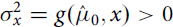 $\sigma _x^2 = g({\hat \mu _0},x) \gt 0$
. Higher values of
$\sigma _x^2 = g({\hat \mu _0},x) \gt 0$
. Higher values of
 $\sigma _x^2$
means that the prediction is less credible. I denote the discounting function
$\sigma _x^2$
means that the prediction is less credible. I denote the discounting function
 $g( \cdot )$
. I follow the convention in the literature (e.g. Bartels Reference Bartels2002; Bullock Reference Bullock2009; Gerber and Green Reference Gerber and Green1999) and assume that the variance of the message is known and that both the prior and the prediction are normally distributed. We can then express the updated belief,
$g( \cdot )$
. I follow the convention in the literature (e.g. Bartels Reference Bartels2002; Bullock Reference Bullock2009; Gerber and Green Reference Gerber and Green1999) and assume that the variance of the message is known and that both the prior and the prediction are normally distributed. We can then express the updated belief,
 ${\hat \mu _1}$
, as
${\hat \mu _1}$
, as
 $${\hat \mu _1}(x) = {\hat \mu _0}\left( {{{g({{\hat \mu }_0},x)} \over {\sigma _0^2 + g({{\hat \mu }_0},x)}}} \right) + x\left( {{{\sigma _0^2} \over {\sigma _0^2 + g({{\hat \mu }_0},x)}}} \right),$$
where
 $\sigma _0^2$
is the strength of the prior belief. The updated belief is, thus, a weighted average of the prior belief and the new information.
$\sigma _0^2$
is the strength of the prior belief. The updated belief is, thus, a weighted average of the prior belief and the new information.
Suppose that a political actor wants to maximize the value of the posterior belief,
 ${\hat \mu _1}(x)$
. What is the optimal prediction, x? This crucially depends on the type of prior discounting that voters engage in. Similar to Mullainathan and Shleifer (Reference Mullainathan and Shleifer2005) and Rabin and Schrag (Reference Rabin and Schrag1999), I exogenously determine how voters perceive predictions conditional on the distance to their priors. I argue that voters can process predictions in principally three different ways. As an example, consider US President Trump’s statement that joining the Trans-Pacific Partnership (TPP) would “ship millions more of our jobs overseas.”
Footnote 5
First, voters may take this statement at face value and update toward the new information unconditional of the distance between their prior beliefs and the prediction (no discounting). The distance between the prior and the prediction does not affect the perceived credibility of the prediction. Second, voters may update toward the new information, but may update less as the distance between the prior and the prediction increases (linear discounting). Third, voters with priors close to the prediction may update, whereas voters with priors far from the prediction may increasingly rely on their prior belief as the distance grows (exponential discounting). After a certain distance, these voters may find the prediction non-credible to such a degree that the prediction backfires and induces them to update less as the prediction grows even more extreme.
Footnote 6
That is, the prediction becomes self-defeating.
${\hat \mu _1}(x)$
. What is the optimal prediction, x? This crucially depends on the type of prior discounting that voters engage in. Similar to Mullainathan and Shleifer (Reference Mullainathan and Shleifer2005) and Rabin and Schrag (Reference Rabin and Schrag1999), I exogenously determine how voters perceive predictions conditional on the distance to their priors. I argue that voters can process predictions in principally three different ways. As an example, consider US President Trump’s statement that joining the Trans-Pacific Partnership (TPP) would “ship millions more of our jobs overseas.”
Footnote 5
First, voters may take this statement at face value and update toward the new information unconditional of the distance between their prior beliefs and the prediction (no discounting). The distance between the prior and the prediction does not affect the perceived credibility of the prediction. Second, voters may update toward the new information, but may update less as the distance between the prior and the prediction increases (linear discounting). Third, voters with priors close to the prediction may update, whereas voters with priors far from the prediction may increasingly rely on their prior belief as the distance grows (exponential discounting). After a certain distance, these voters may find the prediction non-credible to such a degree that the prediction backfires and induces them to update less as the prediction grows even more extreme.
Footnote 6
That is, the prediction becomes self-defeating.
I illustrate this in Figure 1. I plot the effect of a prediction, x, on the updated belief,
 ${\hat \mu _1}$
, for three different discounting functions. The upper row of Figure 1 shows the effect of a prediction, x, on the posterior belief,
${\hat \mu _1}$
, for three different discounting functions. The upper row of Figure 1 shows the effect of a prediction, x, on the posterior belief,
 ${\hat \mu _1}$
, as a function of the distance between the prior belief and the prediction. The bottom row shows the perceived variance of the prediction,
${\hat \mu _1}$
, as a function of the distance between the prior belief and the prediction. The bottom row shows the perceived variance of the prediction,
 $\sigma _x^2$
, as a function of the same distance. In the left column, voters do not exhibit confirmation bias and the perceived variance of the prediction does not depend on the distance between the prior and the prediction. This is evident in the bottom row where the perceived variance is constant. Consequently, marginal persuasion, i.e. the change in persuasion
$\sigma _x^2$
, as a function of the same distance. In the left column, voters do not exhibit confirmation bias and the perceived variance of the prediction does not depend on the distance between the prior and the prediction. This is evident in the bottom row where the perceived variance is constant. Consequently, marginal persuasion, i.e. the change in persuasion
 $({\hat \mu _1} - {\hat \mu _0})$
due to the marginal change in prediction distance
$({\hat \mu _1} - {\hat \mu _0})$
due to the marginal change in prediction distance
 $(x - {\hat \mu _0})$
, is constant over the domain of x. In the center and right columns, voters exhibit two different types of confirmation bias. This can be seen in the bottom row where the perceived variance of the prediction increases with the distance between the prior and the prediction. In the center column, the variance of x grows linearly as the distance between the prediction and the prior belief increases. In the right column, the variance grows exponentially with the distance. In the top row, we see that under confirmation bias, marginal persuasion decreases as predictions grow extreme. However, while marginal persuasion approaches zero under linear discounting, marginal persuasion eventually becomes negative under exponential discounting. Thus, under strong forms of confirmation bias, extreme predictions are self-defeating. When predictions grow extreme, they are deemed very uncertain by voters, who instead rely on their prior beliefs and update little. Proposition 1 formalizes this.
$(x - {\hat \mu _0})$
, is constant over the domain of x. In the center and right columns, voters exhibit two different types of confirmation bias. This can be seen in the bottom row where the perceived variance of the prediction increases with the distance between the prior and the prediction. In the center column, the variance of x grows linearly as the distance between the prediction and the prior belief increases. In the right column, the variance grows exponentially with the distance. In the top row, we see that under confirmation bias, marginal persuasion decreases as predictions grow extreme. However, while marginal persuasion approaches zero under linear discounting, marginal persuasion eventually becomes negative under exponential discounting. Thus, under strong forms of confirmation bias, extreme predictions are self-defeating. When predictions grow extreme, they are deemed very uncertain by voters, who instead rely on their prior beliefs and update little. Proposition 1 formalizes this.
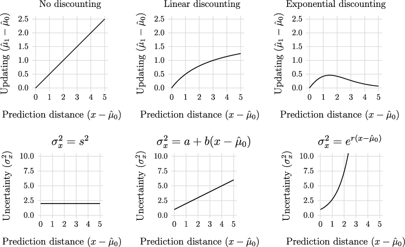
Figure 1 Confirmation Bias Affects the Persuasiveness of Extreme Messages.
Notes:
 $s,a,b,r \gt 0.$
For simplicity, I let
$s,a,b,r \gt 0.$
For simplicity, I let
 ${\hat \mu _0} = 0$
and
${\hat \mu _0} = 0$
and
 $x \ge 0$
. Updating is the difference between the posterior belief and the prior belief. Prediction distance is the difference between the prediction and the prior belief.
$x \ge 0$
. Updating is the difference between the posterior belief and the prior belief. Prediction distance is the difference between the prediction and the prior belief.
Proposition 1
Let the prior,
 ${\hat \mu _0}$
, and the prediction, x, be normally distributed and assume the variance of x to be known and discounting continuous. If discounting is constant, marginal persuasion is constant and persuasion is not bounded as
${\hat \mu _0}$
, and the prediction, x, be normally distributed and assume the variance of x to be known and discounting continuous. If discounting is constant, marginal persuasion is constant and persuasion is not bounded as
 $x \to \infty $
. If discounting is linear, marginal persuasion is positive but decreasing in x and persuasion is bounded as
$x \to \infty $
. If discounting is exponential, persuasion is unimodal and tends to 0 as
$x \to \infty $
.
$x \to \infty $
. If discounting is linear, marginal persuasion is positive but decreasing in x and persuasion is bounded as
$x \to \infty $
. If discounting is exponential, persuasion is unimodal and tends to 0 as
$x \to \infty $
.
Proof. See appendix.
The proposition informs us that there is a fundamental difference between different types of confirmation bias. This has important consequences for the strategy of political actors and implies three different empirical patterns. If voters do not discount the predictions, marginal persuasion will be constant. If voters discount linearly, marginal persuasion will be positive but decreasing. If voters discount exponentially, marginal persuasion will be unimodal. Consequently, under confirmation bias,
Hypothesis 1 extreme predictions are either bounded or self-defeating,
because
Hypothesis 2 the perceived credibility of the predictions decrease as the distance between the prior and the predictions increase.
These empirical patterns correspond to three different polynomial models and I use this to formalize the hypothesis tests. Table 1 shows the expected signs of the regression coefficients for different orders of distance, the magnitude of the difference between the prior belief,
${\hat \mu _0}$
, and the prediction, x. As in Figure 1, I assume that the predictions are greater than than the prior beliefs, meaning that positive updating implies following the prediction.
Footnote 7
The first three columns of the table shows the expectations for updating. Updating under no discounting is constant and corresponds to a linear model. Updating under linear discounting exhibits diminishing marginal effects, corresponding to a quadratic model. Exponential discounting implies a cubic model, since updating is unimodal.
Table 1 Formalization of Hypotheses for Updating and Credibility

Notes: Distance is the magnitude of the difference between the prior belief and the prediction. The expectations are derived assuming that the predictions are greater than the prior beliefs. The dots refer to nonsignificant coefficients, while + and − refer to significant positive and negative coefficients.
The last three columns show the expectations for credibility perceptions. If voters do not discount, there will be no effect of distance on perceived credibility, whereas under linear discounting perceived credibility decreases linearly and under exponential discounting it decreases nonlinearly.
Experimental design
I test the hypotheses with a survey experiment, examining how respondents update their beliefs when they are exposed to a prediction about the outcome of a political reform. I focus on the effect of an economic policy proposal from the US debate, i.e. to join a free trade agreement, the TPP, on manufacturing employment. Figure 2 illustrates the logic behind the treatment and key measurement. The figure shows a voter’s prior belief about a policy outcome,
${\hat \mu _0}$
, a prediction, x, the posterior belief,
${\hat \mu _1}$
, and the distances between the prior belief and these two variables, denoted
 $d( \cdot )$
, on some outcome space, Ω.
$d( \cdot )$
, on some outcome space, Ω.
Treatment and identification problem
The treatment consists of manipulating the distance between the respondent’s prior belief and the prediction,
 $d({\hat \mu _0},x)$
in Figure 2. I refer to this treatment as the prediction distance. This means that respondents are not assigned to predictions but to distances between their prior belief and the prediction. The prediction that respondents are exposed to is the sum of the prior belief and the prediction distance,
$d({\hat \mu _0},x)$
in Figure 2. I refer to this treatment as the prediction distance. This means that respondents are not assigned to predictions but to distances between their prior belief and the prediction. The prediction that respondents are exposed to is the sum of the prior belief and the prediction distance,
 ${\hat \mu _0} + d({\hat \mu _0},x)$
. For example, suppose that the respondent has a prior belief that joining the TPP will lead to a decrease of 0.5 million manufacturing jobs,
${\hat \mu _0} + d({\hat \mu _0},x)$
. For example, suppose that the respondent has a prior belief that joining the TPP will lead to a decrease of 0.5 million manufacturing jobs,
 ${\hat \mu _0} = 0.5$
, and is randomly assigned to a prediction distance of 0.8,
${\hat \mu _0} = 0.5$
, and is randomly assigned to a prediction distance of 0.8,
 $d({\hat \mu _0},x) = 0.8$
. The prediction presented to the respondent is then
$d({\hat \mu _0},x) = 0.8$
. The prediction presented to the respondent is then
 ${\hat \mu _0} + d({\hat \mu _0},x) = 0.5 + 0.8 = $
1.3 million jobs lost.
${\hat \mu _0} + d({\hat \mu _0},x) = 0.5 + 0.8 = $
1.3 million jobs lost.
By defining the treatment as the distance between the prior and the prediction, I ensure that the absolute distance between them is exogenous to the distribution of priors among the respondents. This would not be the case if respondents were randomly assigned to predictions. If, for example, only best guess predictions were used in the experiment, the prediction distance would risk being endogenous to the priors of the respondents. On average, less informed respondents may have prior beliefs further from the best guess. If these respondents also have weaker priors than well-informed respondents, they will be more susceptible to persuasion. This would lead us to erroneously infer that the persuasiveness of predictions increases with the distance between the prior and the prediction.
Outcomes
I examine how the distance between the prior and the prediction affects two outcomes. The first and principal outcome is updating, measured as the difference between the prior and posterior belief. This is shown as
 $d({\hat \mu _0},{\hat \mu _1})$
in Figure 2. I measure the respondents’ beliefs about the effects of the reform using a slider, ranging from −12.3 million to 12.3 million manufacturing jobs in increments of 0.1 million.
$d({\hat \mu _0},{\hat \mu _1})$
in Figure 2. I measure the respondents’ beliefs about the effects of the reform using a slider, ranging from −12.3 million to 12.3 million manufacturing jobs in increments of 0.1 million.
The second outcome is perceived credibility of the prediction, which drives the empirical implications from the theoretical model. I measure perceived credibility of the prediction on an 11-point scale ranging from “not at all credible” to “very credible.” The full question wordings are available in Section D.6 of the appendix.
Case and treatment domain
It is crucial for the validity of the experiment that the prediction distances used as treatments are of such magnitude that any discounting will reveal itself. For example, in Figure 1, if only prediction distances up to 1.5 distance units were used, the discounting in the center and right column would be hard to detect. The prediction distances used in the experiment ranges from 0 to 3 million jobs lost in increments of 0.1 million. The most extreme prediction distance corresponds to twice the job loss in the aftermath of the 2008 economic crisis. Thus, the set of prediction distances includes both extreme and non-extreme values.
I only use negative prediction distances in the experiment because negative and positive predictions, relative to the respondent’s beliefs, do not necessarily have symmetric effects. This complicates the modeling and identification of treatment effects. For example, if predictions in both directions were used, and the dependent and independent variables were operationalized as absolute distances, I would not be able to distinguish updating toward the new information from backfire effects.
Treatment administration
To examine how the predictions affect updating, I need measurements of both the prior and posterior beliefs. Similar to, e.g. Hill (Reference Hill2017), I measure prior beliefs, administer the treatment and measure posterior beliefs in the same survey. Some studies, e.g. Guess and Coppock (Reference Guess and Coppock2020), measure the prior and administer the treatment in separate surveys to avoid priming the prior. However, since the mechanism of interest in this study is the discounting of new information conditional on prior beliefs, priming the prior is not a threat to the validity of the study. Collecting information on priors and posteriors and administering the treatment in the same survey further circumvents the issues of panel attrition and respondents changing their priors between the waves, which would attenuate and possibly confound the estimated treatment effects.
Before the respondents are asked about their priors, they are presented with a vignette and a graph. The vignette informs the respondents that there is disagreement in the public debate about the effect of joining the TPP on manufacturing employment. Together with the graph, the vignette also contains information on the development of manufacturing employment over the last 13 years; namely, the lowest and highest levels under this period, plus the current level. The purpose of this is to help respondents make sense of the scale of the outcome variable (Ansolabehere, Meredith, and Snowberg Reference Ansolabehere, Meredith and Snowberg2013). After this, the respondents’ beliefs about the effects of the reform are measured using the same slider which I use to measure the respondents’ prior beliefs. Figure 3 shows the prior preamble.

Figure 2 Illustration of Treatment and Principal Outcome.
Notes:
${\hat \mu _0}$
is the prior belief,
${\hat \mu _1}$
is the posterior belief, and x is the prediction.

Figure 3 TPP Prior Preamble.
The treatment prediction, equal to the sum of the respondent’s prior and the prediction distance, is presented to respondents in a vignette. I randomize whether the senders are Democrats or Republicans in Congress. The identity of the sender is intentionally sparse on details since confirmation bias should be stronger when individuals have little information for assessing the credibility of the sender (Gentzkow and Shapiro Reference Gentzkow and Shapiro2006). In the main analysis, I average over the effects of Democrat and Republican senders. Randomizing the sender allows me to explore whether partisans discount predictions from their in-group differently as suggested by, e.g. Bartels (Reference Bartels2002) and Bullock (Reference Bullock2009). The TPP is ideal from this perspective since both parties have prominent representatives supporting and opposing the reform, increasing the credibility of the treatment. In Section D.5 of the appendix, I provide all treatment texts.
Sampling and respondent restrictions
Approximately 4,000 respondents were sampled using Lucid, an online exchange for survey responses. Coppock and McClellan (Reference Coppock and McClellan2019) find that both experimental findings and distributions of demographic variables on convenience samples from Lucid closely resemble nationally representative US benchmarks. With 4,000 respondents, the experiment has enough statistical power to identify treatment effects less than .1 standard deviation of the outcome depending on the type of discounting. To ensure that respondents are attentive to the survey content, I only include respondents that pass two pre-treatment attentiveness screeners in the analysis (Berinsky, Margolis, and Sances Reference Berinsky, Margolis and Sances2014). In Section E of the appendix, I present the full power analysis and in Section D.3 I provide the details on the screeners and how I handle missing values.
Analysis and results
I test the hypotheses in two ways. First, I plot how much the respondents’ update, defined as the difference between the posterior and the prior belief, against the prediction distance, defined as the difference between the prior belief and the prediction, and fit a Loess curve to the data. This is shown in Figure 4. Since the three forms of discounting (none, linear, and exponential) correspond to three distinct patterns in updating, the shape of the Loess curve will be informative of whether respondents exhibit confirmation bias and, if they do, what type. No discounting implies a linear relationship between the prediction distance and the distance updated. Linear discounting implies decreasing but positive marginal persuasion. Exponential discounting implies a non-monotonic relationship between prediction distance and the distance updated.

Figure 4 Loess Curves of Updating.
Notes: x is the prediction,
${\hat \mu _0}$
the prior belief, and
${\hat \mu _1}$
the posterior belief. Prediction distance is the distance in millions of jobs between the respondent’s prior and the treatment prediction. Updating is the difference between the posterior and prior belief in millions of jobs. Points show the average updating of all respondents for each value of the treatment variable.
The left panel of the figure shows the Loess curve estimated on the full sample. Footnote 8 The dots show average updating for each value of the treatment variable. The posterior beliefs are more pessimistic than prior beliefs, yet the relatively large confidence interval suggests that there is no obvious treatment effect. However, a closer analysis shows that this null finding is entirely driven by the surprisingly strong negative updating by the respondents who were assigned to the null prediction distance treatment. This group, whose average updating is shown by the left-most point in the graph, received predictions identical to their prior beliefs. Footnote 9 Excluding these respondents from Loess estimation (105 respondents or 2.5% of the sample), shown in the right panel, reveals a discounting pattern clearly consistent with linear discounting. Respondents follow the prediction at first, but when the prediction distance exceeds 1.5 million jobs, the respondents halt their updating.
The null prediction distance differs from all other treatment values since it is the only treatment value that implies no difference between the prior and the prediction. This may explain the surprising effect of this treatment, although it is unclear why this induces strong negative updating among respondents.
The Loess curves suggest that respondents discount extreme predictions, yet, interpreting its shape is a matter of some subjectivity. Therefore, I perform a set of formal hypothesis tests. I model the different discounting patterns with a linear, quadratic and cubic polynomial regression, respectively, and base the model selection on classical hypothesis tests and model fit as indicated by the AIC score. Footnote 10 No discounting is tested by the linear regression, while linear and exponential discounting are, respectively, tested by the quadratic and cubic regression. Table 1 shows the formal expectations, but note that the predictions in the experiment are pessimistic relative to the respondent’s priors and the expectations for updating are thus negated compared to the table. In the regression, distance ranges from 0 to 3, where a 0.1 unit increase corresponds to a prediction distance of 0.1 million jobs lost, and updating is simply the unscaled difference between the posterior and the prior belief in millions of manufacturing jobs. All models are estimated using ordinary least squares with robust standard errors. Due to the curious effect of the null prediction distance, I also estimate these models including a dummy for the null prediction distance. Footnote 11 I present the results in Table 2.
Table 2 Effect of Prediction Distance on Updating and Uncertainty

Notes: OLS estimates with robust standard errors are within parentheses. Prediction distance ranges from 0 to 3, in increments of 0.1 corresponding to a loss of 100,000 jobs. Updating is the difference between the posterior and prior beliefs expressed in millions of jobs. Credibility ranges from 0 to 10 and higher values mean more credible predictions.
*p < 0.05,** p < 0.01,***p < 0.001.
The first three columns of Table 2 show the regressions from the preregistered specifications. None of the individual coefficients are significant, suggesting little effect of the treatments on updating. In columns four–six, I add a dummy indicating the null prediction distance. This reveals an updating pattern clearly consistent with linear discounting. While the coefficient from the linear specification is not significant and only one of the coefficients from the cubic regression is significant, both coefficients from the quadratic regression are significant and have the expected signs. The quadratic regression also has the lowest AIC score and, thus, the best model fit, although the difference is quite small. When the prediction distance is small, respondents follow the prediction. However, as the prediction distance grows, the respondents update less for every increase in prediction distance. Persuasion is maximized when the prediction distance is 1.9, i.e. 1.9 million jobs, corresponding to a decrease of 0.54 million jobs of the posterior beliefs compared to the prior beliefs. If, instead, prediction distance is maximized, the expected updating is a decrease of 0.42 million jobs. Consistent with the first hypothesis, extreme predictions are clearly bounded.
The mechanism driving the patterns of updating is the voter assessment of the credibility of predictions based on the prediction distance. Under no confirmation bias, there should be no effect of prediction distance on perceived credibility of the predictions. Under weak confirmation bias, the effect should be linear and, under strong confirmation bias, the effect should be exponential. I test this by regressing perceived credibility of the predictions, ranging from 0 (not at all credible) to 10 (very credible), on a linear and quadratic specification. Table 1 shows the formal expectations. Again, I include a dummy for null prediction distance for one set of the models. The results are shown in the last four columns of Table 2.
The effect of prediction distance is highly significant, both in the linear and the quadratic specification. The results show that, as the prediction distance grows, respondents deem the predictions less credible. However, instead of credibility decreasing exponentially, the effect of prediction distance tapers off after a prediction distance of 2.1 million jobs. Based on the quadratic model, which also has the best fit according to the AIC score, credibility is minimized when the prediction distance is approximately 2, i.e. 2 million jobs, decreasing credibility by 0.65 scale steps or 0.25 standard deviations compared to the most credible prediction. This effect is robust to excluding the dummy for the null prediction distance. Respondents rely on their prior beliefs when assessing the credibility of information, consistent with the second hypothesis.
I summarize the findings in Figure 5. The figure shows the results of regressing updating, credibility, and support for TPP on the prediction distance variable partitioned into six dummies. Footnote 12 Across the three outcomes, it is evident that beliefs about the effect of the reform do not map one-to-one onto support for the reform. Predictions close to voters’ priors are perceived as credible but do not necessarily shift beliefs, or if they do, do not shift them enough to shift support for the reform. Predictions far from voter’s priors may actually shift beliefs, but are not perceived as credible enough to shift support. For a politician who wants to sway public opinion, the message is clear: predictions have to be spaced just right to effectively change public opinion. A partisan heterogeneity analysis, presented in Section C.5 of the appendix, suggests that this pattern holds regardless of the senders are from the respondents’ favored party or not, but that the discounting of out-group senders begins at smaller prediction distances.

Figure 5 Non-Continuous Effects on Updating, Perceived Credibility, and Support.
Notes: Results are from least squares regressions with robust standard errors. [0,5] is the reference category. Thin lines show 95% confidence intervals and thick lines 90% confidence intervals. Support was measured on a seven-point Likert scale. See the note in Table 2 for a description of updating, credibility and prediction distance.
Finally, the average treatment effects summarized here mask considerable heterogeneity. For example, approximately 20% of the sample do not respond to the treatment at all, while 8% follow the predictions almost perfectly. Footnote 13 In Section C.3 of the appendix, I provide the details of a bounding exercise, which gives further insights into these proportions. In sum, the analysis suggests that even for strong discounting effects, meaning that discounting respondents increasingly rely on their prior instead of the information in the prediction as the prediction distance grows, more than 50% of respondents discount. This exercise suggests that voter discounting is not a marginal phenomenon but may apply to a majority of voters.
Conclusion
Political actors who want to influence the beliefs and preferences of voters face a trade-off. If the predictions lie too close to the beliefs of voters, they may be credible but do little to shift beliefs. If predictions are too extreme, voters may dismiss them as hyperbole and, again, update little. To maximize persuasion, should politicians moderate or exaggerate their predictions? The findings from a preregistered experiment show that voters do not take the statements from politicians at face value, but assess the credibility of new information based on their prior beliefs. Extreme messages are self-defeating because voters assess them as non-credible. Voters, thus, exhibit confirmation bias. The findings imply that politicians are more constrained by the prior beliefs of voters than what existing research suggests (e.g. Bisgaard and Slothuus Reference Bisgaard and Slothuus2018; Broockman and Butler Reference Broockman and Butler2017; Lenz Reference Lenz2013) and must take the beliefs of the electorate into account when crafting their messages. This has two important implications.
First, knowing the electorate’s beliefs are key for crafting effective messages. This justifies the effort made by political actors to survey and map the preferences and beliefs of the electorate. Second, shifting the electorate’s beliefs is not only a powerful tool for shaping public opinion, but a way to indirectly affect the messaging of political competitors. There may be a significant first-mover advantage in shaping voter beliefs (Rabin and Schrag Reference Rabin and Schrag1999). By moving first and shaping the beliefs of voters, a political actor may be able to recenter the rhetoric of a debate or a campaign since all political actors must act strategically with respect to the beliefs of voters.
These findings raise an important question about persuasive strategy for future research. It is crucial for political actors to space their predictions just right to influence voter beliefs. Yet, in reality, the location of the optimal message is unknown. Should politicians take risks or err on the side of caution when issuing their predictions? This depends on whether adverse effects on the credibility of extreme messages spillover on the source itself. If it does, this would induce political actors to moderate their messages even further. However, if the credibility effects are isolated to the message itself, political actors are instead encouraged to take risks when crafting their messages.
Lastly, this study suggests that the adverse effects of confirmation bias on politics are exaggerated. First, confirmation bias does not imply that voters do not learn from new information. The findings show that voters do not refuse to learn, but may assimilate predictions and update their support if the predictions are not too extreme. Second, contrary to what some scholars claim (e.g. Kahan Reference Kahan, Scott and Kosslyn2016), confirmation bias does not imply that voters are irrational even if their goal is to form accurate beliefs. As argued by Gentzkow and Shapiro (Reference Gentzkow and Shapiro2006), when the credibility of the source is uncertain, it is rational for voters to rely on their prior beliefs to infer the credibility of the source. Despite its important implications for, for example, democratic accountability, we do not know whether confirmation bias reflects an unwillingness of voters to learn inconvenient truths or a sophisticated use of heuristic reasoning (Peterson and Iyengar Reference Peterson and Iyengar2020). This is an important endeavor for future research.
Supplementary Material
To view supplementary material for this article, please visit https://doi.org/10.1017/XPS.2021.21.
Data Availability
The data, code, and any additional materials required to replicate all analyses in this article are available at the Journal of Experimental Political Science Dataverse within the Harvard Dataverse Network, at: doi:10.7910/DVN/0WGIJ8. The pre-registration is available at the Open Science Foundation: https://osf.io/vk8am/?view_only=0c98320033f34ca9a2443042f620e273
Acknowledgements
I am grateful to Mattias Agerberg, Vin Arceneaux, John Bullock, Andrej Kokkonen, Peter Loewen, Vincent Pons, Mikael Persson, Martin Vinæs Larsen, Rune Slothuus, an anonymous reviewer, and participants at the Nordic Workshop for Political Behavior 2020 for their helpful comments.
Conflict of Interests
The author has no conflict of interest to declare. Support for this research was provided by the Lars Hierta Foundation and the Helge Ax:son Johnson Foundation.


 Open access