





Introduction
The use of drones in conventional measurement applications represents a potentially revolutionary step. Such applications include the investigation of mobile network electromagnetic (EM, Abbreviations: see Appendix B) exposure, performance, and compliance with public-health limits in the vicinity of high-voltage transmission systems [Reference Paniagua-Sánchez, Marabel-Calderón, García-Cobos, Gordillo-Guerrero, Rufo-Pérez and Jiménez-Barco1–Reference Boukabou and Kaabouch3]. The evaluation of network parameters – which previously had to be carried out on foot or using passenger vehicles – can gain a new dimension. Measurements are required for the planning, commissioning, and capacity verification of cellular networks, and these can be executed with the aid of drones [Reference Kandregula, Zaharis, Ahmed, Khan, Loh, Schreiber, Serres and Lazaridis4–Reference Colombi, Joshi, Xu, Ghasemifard, Narasaraju and Törnevik6]. With unmanned aerial vehicles (UAVs), the time required for measurement can, in many cases, be reduced, since overflying a given area with a drone is considerably simpler and faster than traversing it on foot or by other vehicles [Reference Paniagua-Sánchez, Marabel-Calderón, García-Cobos, Gordillo-Guerrero, Rufo-Pérez and Jiménez-Barco1]. In addition, many areas are difficult to access. This approach also enables the investigation of hazardous locations while reducing risks to personnel.
However, propagation of EM waves depends strongly on environmental conditions and obstacles [Reference Dudnik, Presnall, Tyshchenko and Trush7, Reference Soo, Lim, Chee, Lim and Yap8]. Consequently, measured field strength or received power may vary over time, even at a fixed spatial location [Reference Polak, Kufa, Sotner and Fryza9]. During measurements, such variations do not always pose a problem, since the field strength at a given position in space characterizes that specific location – even when the operation is not a radio frequency electromagnetic field (RF-EMF) measurement but a conventional mobile communication measurement. However, this study examines both the potential advantages and disadvantages of employing a UAV as a measurement platform, particularly for measurements conducted within mobile frequency bands [Reference García-Cobos, Paniagua-Sánchez, Gordillo-Guerrero, Marabel-Calderón, Rufo-Pérez and Jiménez-Barco2, Reference Kandregula, Zaharis, Ahmed, Khan, Loh, Schreiber, Serres and Lazaridis4, Reference Badi, Wensowitch, Rajan and Camp10]. In this frequency range, the UAV may act as a parasitic element due to its conductive carbon-fiber (CF) structure. This effect becomes significant when the UAV is located in the reactive near-field of the receiving antenna. This interaction can introduce impedance mismatch and detuning effects, which may distort the measured field strength and received power [Reference Patil and Arnold11]. As a result, the recorded values may deviate from those representing the typical EM environment of normal mobile network operation. Therefore, this study quantifies the impact of the UAV platform on measurement accuracy, particularly with respect to acceptable uncertainty limits [Reference Kandregula, Zaharis, Ahmed, Khan, Loh, Schreiber, Serres and Lazaridis4]. Furthermore, it must be emphasized that any observed effects are inherently dependent on the specific UAV platform, airframe geometry, antenna configuration, and measurement conditions, and therefore should not be generalized without further validation.
The research focuses on examining the conductive CF frame structure of the UAV intended for use during measurement operations. Fundamentally, even the physical mounting of the measuring instrument can significantly influence the accuracy of the recorded results [Reference Joseph, Aerts, Vandenbossche, Thielens and Martens12]. The proximity of the CF frame introduces capacitive and inductive parasitic coupling, which degrades the uniformity of the receive antenna’s field distribution, induces phase-front distortions, and generates cross-polarization components. This occurs because the frame may alter the local boundary conditions of the receiving antenna, thereby potentially compromising the assumptions associated with far-field measurement conditions. Consequently, the system behaves as though the effective electrical aperture of the combined antenna – environment configuration were enlarged, leading to the violation of far-field measurement conditions and the emergence of near-field-type fluctuations [Reference Núñez, Orgeira-Crespo, Ulloa and García-Tuñón5, Reference Badi, Wensowitch, Rajan and Camp10]. Moreover, reflection, absorption, and scattering effects caused by the UAV body may introduce additional interference phenomena that require investigation, as they may adversely affect measurement accuracy [Reference Boukabou and Kaabouch3]. This issue is explored in detail throughout the study. As an initial hypothesis, it can be stated that when the measurement antennas are properly positioned, these parasitic effects are expected to remain negligible.
The primary objective of the research is to evaluate the suitability of UAV platforms for RF-EMF and received power measurements in mobile communication bands under controlled laboratory conditions. The developed experimental methodology investigates how the placement of the receiving antenna relative to the UAV structure influences the measured EM quantities and whether appropriate antenna positioning can reduce the effects induced by the platform. The study also examines whether the investigated UAV configuration maintains stable far-field measurement conditions during operation. Based on the results obtained, the examined UAV platform [13], including the specific airframe, antenna type, and mounting arrangement, is considered suitable as an auxiliary tool for cellular network RF-EMF assessment and performance evaluation. Thus, the total measurement time can be reduced, and the characterization of otherwise difficult-to-access systems becomes considerably more efficient.
The main contribution of this work is the controlled experimental characterization of UAV-frame-induced perturbation effects on RF-EMF and received power measurements in mobile communication bands. Existing UAV-based RF-EMF studies primarily focus on exposure assessment, propagation mapping, or measurement deployment methodologies [Reference Joseph, Aerts, Vandenbossche, Thielens and Martens12, Reference Ivanov, Muhammad, Tonchev, Mihovska and Poulkov14, Reference Fernandez, Lopez and Andres15], while comparatively limited attention has been devoted to the metrological influence of the UAV platform itself on the measured EM quantities. Studies that address UAV-induced EM effects mainly examine the influence of the drone body on radiation patterns, fading behavior, and polarization response in UAV communication links [Reference Núñez, Orgeira-Crespo, Ulloa and García-Tuñón5, Reference Faul, Korthauer and Eibert16]. Recent UAV-based antenna and propagation measurement literature has further emphasized that measurement accuracy can be affected by platform- and deployment-related factors, including positioning errors, UAV vibrations, airframe shadowing, and potential EM coupling between the UAV body and the mounted antenna [Reference Kandregula, Zaharis, Ahmed, Khan, Loh, Schreiber, Serres and Lazaridis4, Reference Badi, Wensowitch, Rajan and Camp10, Reference Hehenberger, Elmarissi and Caizzone17]. In addition, recent studies on UAV airframe and composite materials indicate that CF or carbon-composite structures may affect antenna radiation characteristics, received signal levels, and polarization behavior [Reference Patil and Arnold11, Reference Wahyudi, Sakti, Prabowo, Hadiyanti, Rahayu, Muzayadah, Wahyudi, Guno, Praludi, Santosa and Sumantyo18]. The present work systematically investigates the influence of antenna-to-airframe spacing under fully anechoic and frequency-resolved laboratory conditions by directly comparing reference and UAV-mounted configurations over the 700–3500 MHz range. The study further quantifies how the conductive CF UAV structure modifies the measured power levels as a function of antenna placement while isolating platform-induced effects from environmental propagation phenomena. The results provide practical integration guidance for UAV-mounted RF-EMF measurement systems employing conductive multirotor platforms.
Naturally, to comprehensively assess the suitability of UAVs as measurement platforms for the aforementioned applications, several additional aspects need to be considered beyond the scope of the present study. These include the EM emission and immunity characteristics of the UAV, as well as dynamic flight-related effects such as rotor-induced scattering and time-varying channel behavior. Such phenomena may introduce additional measurement uncertainty, particularly under real operational conditions [Reference Faul, Korthauer and Eibert16, Reference Zhang, Zhou, Zhang and Qian19, Reference Hou, Wang and Lin20]. However, a full electromagnetic compatibility (EMC) assessment of the UAV is not the objective of this work. From a methodological standpoint, the present study is intentionally focused on experimental characterization. It does not include a full mathematical or numerical EM model of UAV–antenna interactions. Such modeling would require detailed full-wave EM simulations and high-fidelity representation of the complex airframe geometry and material properties. The development of such modeling and simulation-based analyses will be addressed in future phases of the research, alongside a more detailed investigation of emission, immunity, and rotor-induced channel effects.
The remainder of this article is organized as follows. The second section provides an overview of the integration of UAV technology into EM measurement frameworks. In the third section, we give the proposed measurement setup, including the equipment, configurations, and methods. Next, in the fourth section, the measurement results are presented, while the last fifth section draws the conclusions and future work.
State of integration of the UAV technology into EM measurement frameworks
In recent years, the technological evolution of UAVs has fundamentally transformed the methodology of EM measurements and communication system characterization. Early investigations showed that CF UAV structures can interact electromagnetically with communication systems due to their partial electrical conductivity. The so-called “whole-airframe” concepts confirmed that CF structural members are electromagnetically active – capable of providing useful aperture area and controlled coupling that can be exploited in adaptive relay systems [Reference Vidan, Avram, Grigorie, Cican and Nacu21]. However, such structural integration may increase measurement uncertainty, especially when antennas or field probes are placed close to conductive UAV components, where the EM behavior depends on geometry and platform orientation.
In parallel with structural and coupling investigations, significant progress has been achieved in UAV-mounted electromagnetic field (EMF) dosimetry and exposure assessment. Recent research has developed traceable UAV-mounted RF-EMF measurement methodologies that explicitly quantify platform-induced errors and apply standardized flight protocols. One notable study designed and validated a UAV-mounted personal exposimeter system, examining potential interference originating from the UAV’s 2.4 GHz control link and field distortion caused by the airframe. The results demonstrated that the UAV-mounted exposimeter is suitable for validating basestation emissions [Reference García-Cobos, Paniagua-Sánchez, Gordillo-Guerrero, Marabel-Calderón, Rufo-Pérez and Jiménez-Barco2]. At a larger scale, extensive measurement campaigns conducted in urban environments compared ground-based and aerial exposure data. Statistical analyses, including variogram fitting and kriging, showed that mean exposure values measured aloft were slightly higher than those recorded at ground level. However, all results remained well below the International Commission on Non-Ionizing Radiation Protection (ICNIRP, 2020) reference limits. The UAV control link was found to affect only the 2.4 GHz Wi-Fi band, while structural interference could be compensated through calibration, confirming the reliability of UAV-based dosimetry [Reference Paniagua-Sánchez, Marabel-Calderón, García-Cobos, Gordillo-Guerrero, Rufo-Pérez and Jiménez-Barco1]. In parallel, research employing a UAV-mounted software-defined radio (SDR) introduced the volumetric radio environment map (REM) concept. Measurements in the 2.4 GHz ISM band, combined with constellation-based signal processing, enabled the reconstruction of three-dimensional (3D) EMF maps. This approach reduced flight time and post-processing effort while maintaining accuracy [Reference Ivanov, Muhammad, Tonchev, Mihovska and Poulkov14]. Such data-driven REM or VREM (virtual radio environment map) systems substantially reduce computational load compared to classical ray-tracing methods, making them essential for future network planning, coverage optimization, and interference prediction [Reference Shawel, Woldegebreal and Pollin22]. UAV-mounted measurements performed around 5G New Radio (NR) small-cell base stations have been directly linked to compliance evaluation according to the IEC 62232 standard (International Electrotechnical Commission). Field experiments assessed exposure levels at various distances, with results compared to ICNIRP safety limits and mapped to IEC-defined basestation power classes (E2/E10/E100). The use of beamforming significantly reduced non-target, or “bystander,” exposure, providing a realistic assessment of safety margins and clarifying how antenna technology and site classification influence compliance zones [Reference Aerts23].
The application of UAVs in antenna diagnostics and propagation analysis has proven particularly valuable in evaluating complex 4G and 5G network infrastructures. Conventional diagnostic approaches are often costly, time-consuming, and limited by topographical constraints. Experimental results confirmed that UAV-mounted configurations can reconstruct actual antenna radiation patterns with sufficient accuracy, detect antenna misalignments, and support network optimization. Uncertainties arising from multipath reflections and structural scattering were shown to remain manageable when systematic calibration procedures are applied [Reference Fernandez, Lopez and Andres15]. In the domain of high-precision radar calibration, UAV applications present unique challenges, as polarimetric radar systems are extremely sensitive to phase, amplitude, and polarization distortions. Studies have shown that with appropriate probe and platform selection, along with carefully planned flight geometry, UAV-mounted configurations can meet the stringent calibration requirements of polarimetric weather radars [Reference Umeyama, Salazar-Cerreno and Fulton24, Reference Umeyama, Salazar-Cerreno and Fulton25]. Further refinement of UAV-based characterization has been achieved through investigations of the combined effective radiation pattern (CERP), which describes the composite radiation behavior of UAV-mounted antennas. Field experiments demonstrated that the application of CERP can reduce received power prediction errors by up to 10 dB compared to laboratory reference patterns, indicating that only a limited number of calibration flights are required for effective antenna–mount configuration optimization [Reference Rahman, Guvenc, Abrahamson, Mishra and Bhuyan26]. Comprehensive reviews [Reference Kandregula, Zaharis, Ahmed, Khan, Loh, Schreiber, Serres and Lazaridis4] further highlight that UAV-mounted near-field and far-field antenna measurements, when combined with precise positioning (differential global positioning system [DGPS]/real-time kinematic [RTK]) and stable attitude control, can achieve accuracy within the range of 0.5–1 dB.
Overall, these studies demonstrate that UAV-mounted EM measurements provide improved spatial coverage and efficiency, while introducing platform-dependent uncertainties that require careful modeling and compensation. Future research focuses on modeling measurement uncertainty and mitigating EM coupling between the airframe and antennas. It also addresses the development of real-time error compensation techniques. These aspects are essential for ensuring metrological traceability in complex radio environments [Reference Paniagua-Sánchez, Marabel-Calderón, García-Cobos, Gordillo-Guerrero, Rufo-Pérez and Jiménez-Barco1, Reference García-Cobos, Paniagua-Sánchez, Gordillo-Guerrero, Marabel-Calderón, Rufo-Pérez and Jiménez-Barco2, Reference Kandregula, Zaharis, Ahmed, Khan, Loh, Schreiber, Serres and Lazaridis4, Reference Ivanov, Muhammad, Tonchev, Mihovska and Poulkov14, Reference Fernandez, Lopez and Andres15, Reference Vidan, Avram, Grigorie, Cican and Nacu21–Reference Rahman, Guvenc, Abrahamson, Mishra and Bhuyan26].
Proposed measurement method for the effect of the placement of the measuring antenna
Measurement equipment
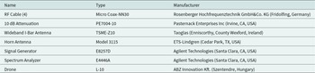
The measuring instruments and auxiliary equipment listed in Table 1 were used to perform the effect of the placement of the measuring antenna tests.

Table 1 Long description
The table inventories measurement equipment, giving each item’s name, its model or type, and the manufacturer with location. It includes four RF cables (Micro Coax-NN30) from Rosenberger in Germany and a ten decibel attenuator (PE7004-10) from Pasternack in the United States. Two antennas are listed: a wideband I-bar antenna (TSME-Z10) from Taoglas in Ireland and a horn antenna (Model 3115) from ETS-Lindgren in the United States. The RF test instruments are a signal generator (E8257D) and a spectrum analyzer (E4446A), both from Agilent Technologies in Santa Clara, California. A drone platform is also included: L-10 from ABZ Innovation in Hungary. The table is descriptive only and does not provide performance specifications, calibration status, or measurement settings for these items.
Measurement setup
The primary consideration in defining the measurement arrangement for EM power level measurements was to minimize disturbing influences during the experiment and thereby ensure the lowest possible measurement uncertainty. Measurements were conducted in an FAC-3 (fully anechoic chamber) shielded test room in order to isolate UAV-platform-induced effects from environmental propagation phenomena. This prevented external signals, such as commercial mobile network transmissions, from interfering with the experiment and increasing uncertainty. It also ensured that the signals radiated during testing did not disturb the live public network. Owing to the properties of the FAC chamber, the absorbers, and the directional characteristics of the horn antenna used for transmission, the interference fading produced by signals arriving from outside the quiet zone can be regarded as negligible [Reference Petzold, Magdowski and Vick31, 32]. Furthermore, any attenuation or reflections in the test-bench signal chain were mitigated using the substitution method: first, a reference was measured with the wideband receiving I-Bar antenna (TSME-Z10) alone, then the measurement was repeated with the drone frame mounted on the same I-Bar antenna [Reference Culotta-Lopez, Skeidsvoll, Costin, Buchi and Espeland33, Reference Badi, Wensowitch, Rajan and Camp34].
The investigated UAV platform is a multirotor CF system with a maximum height of 61 cm, a width of 146 cm, and a depth of 102 cm, representing a typical medium-size industrial UAV platform [13]. The airframe is constructed from carbon-fiber reinforced polymer (CFRP) structural elements. Although a detailed frequency-dependent EM characterization of the composite material was not available, the CFRP structure exhibits partially conductive behavior; effective in-plane conductivities reported for CFRP laminates are commonly on the order of  $10$–
$10$–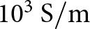 $10^3~\mathrm{S/m}$, while transverse and through-thickness conductivities may be several orders of magnitude lower due to the anisotropic fiber-resin architecture [13, Reference Vidan, Avram, Grigorie, Cican and Nacu21]. Therefore, in the present study, the airframe was treated as an electrically conductive CFRP structure, and its influence on the measured EMF was evaluated experimentally rather than through full material-parameter-based EM modeling. When investigating the interaction between the measurement antenna (I-Bar) position and the drone airframe, it is essential that the entire UAV frame is located within the main beam of the transmitting antenna. This ensures that the measured EMF reflects the influence of the complete airframe. This must be considered especially when a strongly directional transmitting antenna is used during the measurement [Reference Badi, Wensowitch, Rajan and Camp10, Reference Pastorcici, Constantin, Heiman and Tamas35]. In the present arrangement, this condition was satisfied by selecting a sufficient separation distance. The horn antenna beam fully encompassed the UAV structure, taking into account the antenna beamwidth and the overall geometry of the setup. This also reflects realistic operational scenarios, where mobile communication antennas typically exhibit wider beamwidths and, in most cases, illuminate the entire UAV. In determining this distance, the horn antenna beamwidth in the E- and H-planes was considered. This beamwidth varies with frequency but is generally narrow, typically between 40 $^\circ$ and 60 $^\circ$ [30]. For the 700–3500 MHz band, the minimum characteristic beamwidth (40 $^\circ$) and the system geometry were taken into account. The drone maximum lateral dimension is 146 cm (height 61 cm), the length of the receiving I-Bar antenna is 17.6 cm, and the planned maximum antenna–frame separation is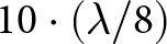 $10\cdot(\lambda/8)$, which corresponds to 53.5 cm at 700 MHz [13, 27, Reference Rappaport36]. Including the 50 cm support stage used in the measurement, the largest overall dimension of the assembled system is therefore 182.1 cm, for which the corresponding minimum required distance is rounded to 250 cm. In addition, the separation between the transmitting horn and the equipment under test (EUT) was chosen so that all measurements are carried out in the far field, as is typically the case in real-world applications. Using the Rayleigh-distance relation
 \begin{equation}
R_d = \frac{2\,(D_T + D_R)^2}{\lambda},
\end{equation}
\begin{equation}
R_d = \frac{2\,(D_T + D_R)^2}{\lambda},
\end{equation}where  $D_T$ (24.4 cm) and $D_R$ (17.6 cm) denote the effective apertures of the transmitting and receiving antennas, respectively, and $\lambda$ is the wavelength, the resulting distance at the band edges is 415 cm [27, 30, Reference Sun, Li, Han, Liu, Xue and Tao37]. Based on these considerations, the transmitter–EUT spacing was set to 450 cm.
Given the present arrangement – within a shielded chamber free of external noise and using a directional transmitting antenna – it is not necessary, over the 700–3500 MHz range, to vary the antenna–EUT distances during the measurement sequence. To avoid any influence on the recorded results, the radio frequency (RF) generator and spectrum analyzer used for received power measurements were placed outside the anechoic chamber.
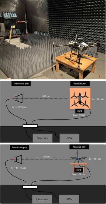
The I-Bar antenna mounted on the UAV is a device typically employed in the parameter and performance testing of cellular base stations. For the UAV-mounted configuration, the receiving antenna was placed at multiple positions and heights in order to emulate how the antenna position and its spacing to the CF airframe affect the measurement outcome. The initial position of the receiving antenna was established on the top of the frame, directly above the largest structural element (the drone body). The initial height of the antenna feed point above the floor was 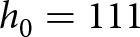 $h_0 = {111}$ cm. In subsequent measurements, the receiving antenna was displaced by predetermined increments away from the drone body, thereby simulating how the antenna–frame separation influences the measured received power. During the investigation, the height of the transmitting horn antenna was fixed at the midpoint between the minimum and maximum heights of the receiving I-Bar antenna (111 and 164.5 cm), i.e., $h_1 = {137.75}$ cm, and remained constant throughout the tests. With the configurations described previously, the examined UAV is placed in the test position shown in Figure 1. The receiving antenna was mounted on the UAV using an electrically non-conductive plastic mast, which was fixed to the frame using two plastic clamps in order to avoid unintended EM interaction with the CF structure. The mast had an outer diameter of 2.5 cm and an unsupported length of 60 cm. This mounting arrangement ensures stable antenna positioning during the measurements and minimizes mechanical perturbations of the measurement geometry.
The test setup: photo, top view, and side view. The transmitting section, including the horn antenna at height  $h_1 = {137.75}$ cm, is located on the left-hand side of the images. The receiver section, including the EUT – which contains UAV and I-Bar antenna – with initial height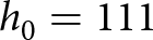 $h_0={111}$ cm from the ground, is located on the right-hand side on a support stage of height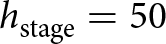 $h_\text{stage} = {50}$ cm. The signal generator (Generator) and the spectrum analyzer (SPA) are located outside the fully-anechoic chamber.

Figure 1 Long description
The image consists of three parts. The first part is a photo showing a test setup in an anechoic chamber. On the left, there is a horn antenna mounted on a stand, surrounded by foam pyramids. On the right, a table holds a drone with an I-Bar antenna mounted on it. The second part is a schematic diagram illustrating the test setup. On the left, labeled ′Emission part,′ is a horn antenna at a height of 137.75 centimeters. A dashed line extends 450 centimeters to the right, connecting to the ′Receiver part,′ which includes the equipment under test (EUT) with a height of 111 centimeters and a stage height of 50 centimeters. Below, a generator and a spectrum analyzer (SPA) are connected to both parts. The third part is another schematic similar to the second, but the UAV is shown with a dashed outline, indicating a different configuration or position. The connections and labels remain consistent across the diagrams, emphasizing the relationship between the emission and receiver sections.
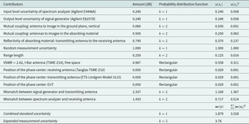
In evaluating measurement uncertainty, not only the directly measured quantities but also all factors that may influence the reliability of the results must be considered. These include calibration certificates, manufacturer specifications, instrument stability and drift, environmental influences, and applicable correction factors. The total measurement uncertainty for the given setup was determined in accordance with the requirements of the relevant standards [38, 39]. Following established procedures in the literature, the Type-B components (non-statistical or evaluated by analytical means) were identified and quantified. The contributing sources and their corresponding uncertainty values are summarized in Table 2. It should be noted that a comprehensive uncertainty evaluation would also require a Type-A (statistical) assessment, involving repeated measurements at identical spatial configurations, repeatability evaluation, and subsequent statistical analysis. As this aspect extends beyond the scope of the present work, the current study focuses primarily on Type-B uncertainty estimation under controlled and quasi-static laboratory conditions. Mechanical positioning effects, including antenna placement and mounting repeatability, were considered within the corresponding uncertainty contributors listed in Table 2. In addition, the manuscript provides a descriptive statistical evaluation of the measured UAV-induced deviations in the section “Processing and evaluation of power measurement data,” based on the complete frequency – spacing – orientation measurement matrix.
Measurement uncertainty budget with the contributors calculated according to [27–30, 38, 39]

Table 2 Long description
The table lists contributors to a measurement uncertainty budget in decibels, giving each contributor’s amount, assumed probability distribution, standard uncertainty, and squared standard uncertainty. The biggest contributor is mismatch between the signal generator and the transmitting antenna: amount 2.337 dB and standard uncertainty 1.169 dB, with the largest squared contribution at 1.367. The next largest is mismatch between the spectrum analyzer and the receiving antenna: amount 1.433 dB and standard uncertainty 0.717 dB, squared contribution 0.514. Random measurement uncertainty is also substantial, with amount and standard uncertainty both 1.000 dB and a squared contribution of 1.000. Other notable contributors include VSWR in free space (amount 0.967 dB, standard uncertainty 0.558 dB) and reflectivity of absorbing material between antennas (amount 0.740 dB, standard uncertainty 0.370 dB). Several smaller terms, such as phase-centre positions and mutual coupling to the ground-plane image, each contribute standard uncertainties around 0.029 to 0.030 dB. The combined standard uncertainty is 1.879 dB, and the expanded measurement uncertainty is 3.76 dB using a coverage factor of 2. Values depend on the stated distribution assumptions and coverage factors, so comparisons should be made within those assumptions.
Instrument configuration signal generator
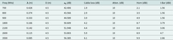
On the signal generator (E8257D), we configured the parameters required for the EM power level investigations. First, the frequency was set to 700 MHz, and the output power was adjusted to compensate for the total path attenuation. Care was taken to keep the output signal sufficiently above the noise floor while not reaching the saturation input at the spectrum analyzer, which is about  $-$10 dBm [Reference Foroughimehr, Wood, McKenzie, Karipidis and Yavari40, 41]. An adequate input attenuator on the receiver side can ensure proper signal levels. However, excessively high generator output levels are not recommended, because the generator’s output impedance can become unstable, which would increase the measurement uncertainty [38, 39, Reference Kim, Yun and Park42]. Therefore, for each test frequency, we determined the total path attenuation, which in this case is the sum of free-space loss
 \begin{equation}
a_0 = 20\log_{10}\!\left(\frac{4\pi D}{\lambda}\right),
\end{equation}
\begin{equation}
a_0 = 20\log_{10}\!\left(\frac{4\pi D}{\lambda}\right),
\end{equation}the cable losses, and the inserted fixed attenuator, together with the antenna gains [Reference Rappaport36]. The numerical values are summarized in Table 3.
Parameters used to determine path loss calculated from [27, 30, Reference Rappaport36]

Table 3 Long description
The table lists frequency-dependent parameters used for path-loss calculations, including wavelength, a fixed distance D, an a0 term in dB, cable loss, a fixed attenuation value, and antenna gains for a horn and an I-Bar. Frequency ranges from 700 to 3500 MHz, and wavelength decreases steadily from 0.428 m at 700 MHz to 0.085 m at 3500 MHz. The distance D is constant at 4.5 m for all rows. The a0 value increases with frequency, from 42.406 dB at 700 MHz to 56.385 dB at 3500 MHz. Cable loss generally increases with frequency, from 1.9 dB at 700 MHz to 6.1 dB at 3500 MHz, with intermediate values such as 3.9 dB at 900 MHz and 5.9 dB at 2600 MHz. The attenuation column is constant at 10 dB across all frequencies. Horn gain increases from 2.1 dBi at 700 MHz to 9.9 dBi at 3500 MHz, while I-Bar gain varies non-monotonically, ranging from 1.56 dBi at 700 to 900 MHz up to 4.7 dBi at 2600 MHz. Interpret values as input parameters rather than measured outcomes, since several columns are fixed or equipment-specific and may not generalize beyond the stated setup.
Instrument configuration spectrum analyzer
During the received power measurements, we employed a frequency-selective measurement method using an Agilent E4446A spectrum analyzer. The instrument was configured as follows. In each case, the center frequency was set to the frequency under test, and the resolution bandwidth (RBW) was 100 kHz, which yields a spectral representation of sufficient detail for the measurements. The video bandwidth (VBW) was set to 300 kHz to obtain an optimal envelope. The input attenuation was 10.0 dB, and the reference level was  $-$10.0 dBm. The RMS detector was used. The sweep time was set to 100 ms to ensure sufficient sampling for averaging. The sweep-averaging count was set to 20. These averaging settings and the use of the RMS detector reduce measurement uncertainty [38, 39, Reference Kim, Yun and Park42–44]. At every spatial position, the recording window was 2 s, ensuring adequate time and sampling depth for averaging.
Measurement method
The measurement campaign was designed to quantify the effect of antenna–airframe separation on the received power measured with the UAV-mounted configuration. For each test frequency, two datasets were acquired under identical instrument conditions: (i) a reference dataset without the UAV in the test volume and (ii) a UAV-mounted dataset with the receiving antenna installed above the airframe.
Reference measurements were performed first. The initial position of the wideband receiving antenna was established on the top of the frame, directly above the largest structural element (the drone body). This configuration represents the most critical case in terms of airframe-induced EM interaction. It maximizes the coupling between the antenna and the UAV structure [Reference Badi, Wensowitch, Rajan and Camp10, 13, Reference Badi, Wensowitch, Rajan and Camp34, Reference Reis, Silva, Albuquerque and Pinho45, 46]. In addition, for the performance and EM exposure studies planned later, mounting the receiving antenna on this flat top surface is also mechanically preferable, simpler to implement, and more robust. Accordingly, in the reference measurements, the wideband receiving antenna was oriented vertically and placed at the starting height 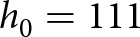 $h_0 = {111}$ cm. The transmitting horn antenna remained vertically polarized at the previously defined height $h_1 = {137.75}$ cm. For each frequency, the receiving side was rotated from $0^\circ$ to $180^\circ$ in $45^\circ$ increments. At each angular position, the received power was recorded over 2 s, and the reported value was taken as the mean over that interval. After completing the measurements at the initial position, the antenna height was increased in discrete steps according to
 \begin{equation}
h_2 = h_0 + h_\text{wb}, \quad \mbox{with }h_\text{wb} = n\cdot \frac{\lambda}{8},
\end{equation}
\begin{equation}
h_2 = h_0 + h_\text{wb}, \quad \mbox{with }h_\text{wb} = n\cdot \frac{\lambda}{8},
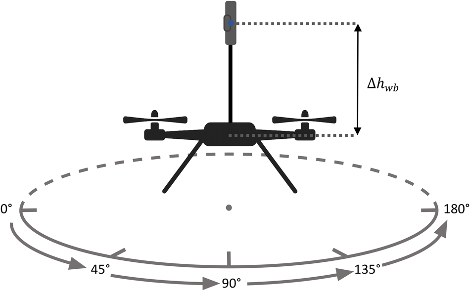
\end{equation}where  $h_\text{wb}$ denotes the spacing between the I-Bar antenna and the drone body, $\lambda$ is the actual wavelength, $n$ is the step index, and $h_2$ is the height of the I-Bar antenna measured from the ground.
In order to avoid undersampling of the standing-wave pattern associated with VSWR, a spatial step of  $\lambda/8$ was adopted as a deliberate oversampling choice. The standing-wave voltage varies sinusoidally in space with a period of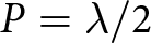 $P=\lambda/2$. According to the Nyquist criterion, preventing spatial aliasing requires a sampling step exceeding $\le P/2=\lambda/4$. By selecting $\lambda/8$, the sampling density is doubled relative to this limit, allowing the characteristic maxima and minima of the field distribution to be resolved reliably across all investigated frequencies. This approach ensures that the spatial variation of the field is accurately captured, including rapid changes and reactive near-field effects in the vicinity of the UAV structure. As a result, peak values can be determined with confidence, and standing-wave-induced measurement uncertainty is effectively reduced [Reference Pelland, Hindman and Newell47, Reference Qureshi, Schmidt and Eibert48]. The configuration of other devices remains unchanged in this case.
The UAV-mounted configurations were then carried out using the same frequencies, antenna polarizations, angular positions, acquisition time, and analyzer settings as in the reference case. The UAV was placed at the test position shown in Figure 1, and the receiving antenna was mounted above the airframe at the same set of heights used for the reference measurements, as shown in Figure 2. This one-to-one correspondence ensures that the difference between the reference and UAV-mounted datasets isolates the effect of the airframe for each frequency, orientation, and antenna–frame separation.
The complete measurement matrix therefore consisted of the following parameters:
- sequence of receive antenna heights ( $h_2$), n: 0; 1; 2; 3; 4; 5; 6; 7; 8; 9; 10
- set of test frequencies [MHz]: 700; 800; 900; 1800; 2100; 2600; 3500
- set of EUT Directions [Degree]: 0; 45; 90; 135; 180
- type of measurements: Reference/UAV.

Measurement procedure of the UAV-mounted configuration method. The separation between the drone frame and the receive antenna (Wideband I-Bar) is varied according to the parameter  $h_\text{wb}$ (3). At each antenna–frame distance position, the orientation of the EUT relative to the transmitting horn antenna is adjusted in five discrete steps, where 0 $^{\circ}$ corresponds to a face-to-face alignment.

Results of EM power level measurements
Processing and evaluation of power measurement data
The evaluation focuses on quantifying the deviation between the reference and UAV-mounted configurations as a function of antenna–frame separation. The generator and spectrum analyzer were configured according to the methodology described in the section “Proposed measurement method for the effect of the placement of the measuring antenna.” After completion of the measurements, the recorded data were processed using a Python (Version 3.12) program. For each measurement condition, the received power was first time-averaged over the recorded interval. The UAV-induced perturbation was then quantified as the absolute received-power difference between the UAV-mounted and reference configurations:
 \begin{equation}
|\Delta P(f,n,\theta)| =
\left|P_{\mathrm{UAV}}(f,n,\theta)-P_{\mathrm{ref}}(f,n,\theta)\right|,
\end{equation}
\begin{equation}
|\Delta P(f,n,\theta)| =
\left|P_{\mathrm{UAV}}(f,n,\theta)-P_{\mathrm{ref}}(f,n,\theta)\right|,
\end{equation}where  $f$ denotes the test frequency, $n$ is the antenna-spacing index defined in section “Proposed measurement method for the effect of the placement of the measuring antenna,” and $\theta$ is the orientation of the EUT relative to the transmitting antenna. Furthermore,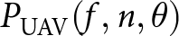 $P_{\mathrm{UAV}}(f,n,\theta)$ and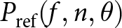 $P_{\mathrm{ref}}(f,n,\theta)$ denote the time-averaged received power levels measured for the UAV-mounted and reference configurations, respectively. Since both datasets were acquired using identical frequencies, antenna-spacing indices, EUT orientations, acquisition times, and instrument settings, Equation (4) provides an estimate of the airframe-induced deviation for each measurement condition.
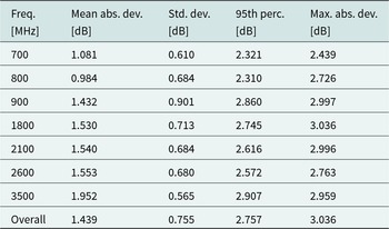
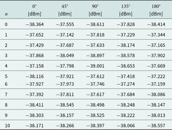
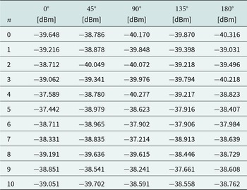
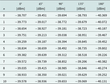
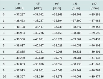
To better quantify the reliability of the measured deviations, a descriptive statistical analysis was performed using the complete set of averaged values reported in Appendix A, in Tables A1–A14. The absolute deviation defined in Equation (4) was evaluated in terms of mean absolute deviation, standard deviation, 95th percentile, and maximum value, as summarized in Table 4. This descriptive analysis characterizes the variability of the measured deviations over the investigated measurement matrix and is distinct from a full Type-A repeatability uncertainty assessment.
Descriptive statistical summary of the absolute received-power deviations between the reference and UAV-mounted configurations

Table 4 Long description
The table summarizes absolute received-power deviations, in decibels, between a reference setup and a UAV-mounted setup across several frequencies. For each frequency it reports the mean absolute deviation, standard deviation, 95th percentile, and maximum absolute deviation. Mean absolute deviation is smallest at 800 MHz (0.984 dB) and 700 MHz (1.081 dB), and increases at higher bands, peaking at 3500 MHz (1.952 dB). The 95th percentile ranges from 2.310 dB at 800 MHz to 2.907 dB at 3500 MHz, indicating that most deviations stay below about 3 dB across bands. Maximum absolute deviation is highest at 1800 MHz (3.036 dB), matching the overall maximum, while other maxima are slightly lower, such as 2.439 dB at 700 MHz and 2.763 dB at 2600 MHz. Variability by standard deviation is greatest at 900 MHz (0.901 dB) and lowest at 3500 MHz (0.565 dB). Overall, the mean absolute deviation is 1.439 dB with a 95th percentile of 2.757 dB, but these summaries do not indicate the direction of the power difference because deviations are absolute.
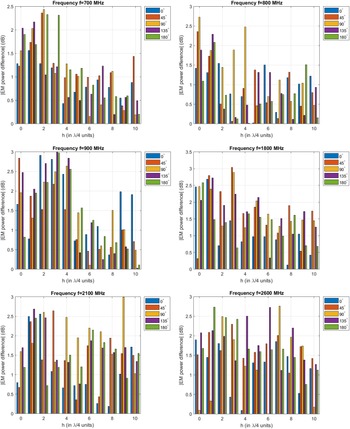
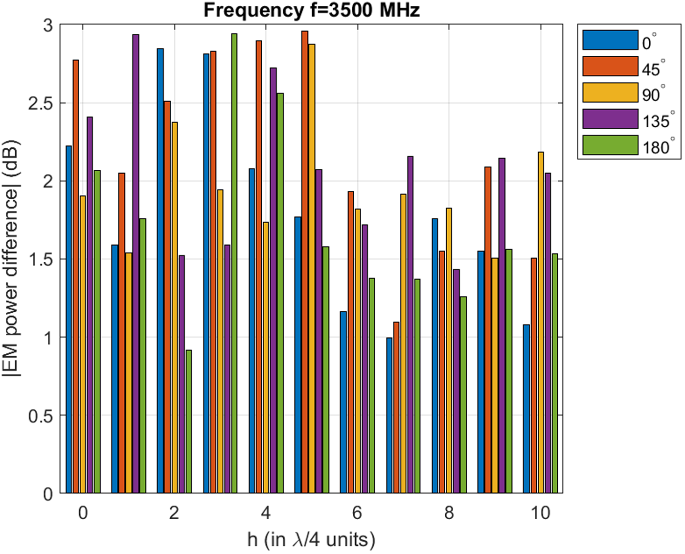
Following this statistical evaluation, the most representative absolute received-power differences are illustrated in Figures 3 and 4 for the investigated 700–3500 MHz low-band and mid-band mobile spectrum. These figures show the differences between the averaged results of the reference and UAV-mounted configurations as a function of antenna–airframe separation and EUT orientation.
Absolute difference in received power between the reference and UAV-mounted configurations for frequencies between 700 and 2600 MHz. The horizontal axis shows the antenna–airframe separation defined by Equation (3), while the vertical axis represents the absolute power difference. The bar colors indicate the orientation of the EUT relative to the transmitting antenna. Blue corresponds to  $0^\circ$ (face-to-face alignment), red to $45^\circ$, yellow to $90^\circ$, purple to $135^\circ$, and green to $180^\circ$. Each subplot represents a different frequency. The results show that the deviations generally decrease as the antenna–airframe separation increases. This trend is more pronounced at lower frequencies, where the physical spacing between measurement points is larger. Most deviations remain within approximately 3 dB.

Figure 3 Long description
The image contains six bar graphs comparing EUT power differences across frequencies from 700 to 2600 megahertz. Each graph shares the same axes: the horizontal axis labeled h (in lambda over 4 units) from 0 to 10 and the vertical axis labeled EUT power difference (decibel) with varying ranges. The legend indicates angles: 0 degree, 45 degree, 90 degree, 135 degree and 180 degree. Graph A (700 megahertz): Power differences generally decrease as h increases, with notable peaks at h equals 2 and 6 for 0 degree and 90 degree. Graph B (800 megahertz): Shows variability with peaks at h equals 3 and 7 for 45 degree and 135 degree. Graph C (900 megahertz): Displays a consistent decrease in power difference, with a peak at h equals 4 for 180 degree. Graph D (1800 megahertz): Exhibits fluctuations, with the highest peak at h equals 5 for 90 degree. Graph E (2100 megahertz): Shows a steady trend with a peak at h equals 8 for 0 degree. Graph F (2600 megahertz): Displays minimal variation, with a peak at h equals 9 for 135 degree. Overall, power differences tend to decrease with increasing h, with more pronounced deviations at lower frequencies. Each graph highlights how different angles affect power differences at specific h values.
Absolute difference in received power between the reference and UAV-mounted configurations at 3500 MHz. The horizontal axis shows the antenna–airframe separation defined by Equation (3), while the vertical axis represents the absolute power difference. The bar colors indicate the orientation of the EUT relative to the transmitting antenna. Blue corresponds to  $0^\circ$ (face-to-face alignment), red to $45^\circ$, yellow to $90^\circ$, purple to $135^\circ$, and green to $180^\circ$. Compared with the low-band cases, the deviation at 3500 MHz exhibits a weaker dependence on spacing, indicating that the airframe influence decays within a shorter absolute distance. The observed deviations remain within approximately 3 dB.

Summary of power measurements results
The results show that the measured power levels in the reference and UAV-mounted configurations are in close agreement (Figures 3 and 4). This observation is also supported by the descriptive statistical summary in Table 4. Across the complete set of evaluated frequency–spacing–orientation combinations, the overall mean absolute deviation was 1.439 dB, with a standard deviation of 0.755 dB. The 95th percentile of the absolute deviation was 2.757 dB, while the maximum observed deviation was 3.036 dB. The absolute differences therefore indicate that the use of the examined UAV does not introduce significant deviations beyond the expected measurement uncertainty bounds. It should be emphasized that this observation is valid for the investigated configuration and cannot be directly generalized to other UAV platforms or antenna arrangements. In other words, the capacitive and inductive parasitic coupling associated with the nearby CF frame does not materially modify the local boundary conditions of the receive antenna, nor does it invalidate the far-field approximation. Accordingly, it does not markedly degrade field uniformity. Under the present conditions, the deviations typically remain within 3 dB relative to the reference measurements. This threshold is consistent with established in-situ RF-EMF measurement practices, where expanded uncertainties of up to 4–6 dB are commonly accepted [Reference Kim, Yun and Park42, 43, 49]. Therefore, the investigated UAV platform can be considered suitable for EM exposure and performance assessment in cellular networks.
From an EM perspective, the conductive CF frame primarily interacts with the incident field through reflection and scattering mechanisms. Owing to the high electrical conductivity of CF composites, a large portion of the incident EM energy is reflected at the surface due to impedance mismatch, while a smaller portion is absorbed or transmitted. The convex and non-planar geometry of the UAV frame redistributes the reflected field into multiple directions, resulting in a spatially dispersed scattered field. Consequently, the contribution of these scattered components at the receiving antenna is significantly lower than that of the direct wave, and their influence decreases with increasing antenna–frame separation.
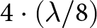
As the spacing between the receive antenna and the UAV frame increases, the absolute deviations relative to the reference measurements decrease. According to the results, this tendency is most prominent at low-band mobile frequencies (700, 800, 900 MHz). A similar tendency is also observable in the mid-band results (1800, 2100, 2600, 3500 MHz), most clearly at 1800 MHz. This frequency-dependent behavior is consistent with the spacing definition  $h_{\mathrm{wb}} = n\cdot(\lambda/8)$. For a given step index $n$, the absolute antenna–frame separation is larger at lower frequencies because the wavelength is longer. The stronger spacing dependence observed in the low-band results therefore reflects the larger physical distance change per step, whereas at mid-band frequencies the same index progression samples a more compact physical region. As the separation increases, both the reactive near-field contribution and the scattered field from the CF structure decay. As a result, the measurement system remains in a stable far-field regime and does not transition into a fluctuating near-field state during the tests. Based on the measurement results, at receive antenna positions located farther than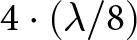 $4\cdot(\lambda/8)$ from the frame, the differences between the reference and UAV-mounted configurations are lower by approximately 1–1.5 dB than at the closer positions. This tendency is also consistent with the observed results in Figures 3 and 4, where the variation of the measured deviations with spacing is more significant at lower frequencies.
However, it is important to note that achieving larger antenna–frame separations requires a mechanically stable mounting structure, particularly under real-world wind conditions. Therefore, aerodynamic design and structural mass must be carefully considered [Reference Ghirardelli, Kral, Cheynet and Reuder50]. Furthermore, the reported deviations were obtained under controlled laboratory conditions. In real environments, additional factors such as interference, intermodulation, and noise may increase the observed differences.
Conclusions and future work
The laboratory measurements confirm the objectives defined at the beginning of this study. The proposed measurement procedure provides a consistent and sufficiently detailed characterization of the differences in EM power level between the reference and UAV-mounted configurations over the investigated frequency range.
The results show that, for the investigated UAV platform, antenna type, mounting arrangement, and FAC conditions, the UAV-mounted configuration does not introduce a practically significant deviation in the received power over 700–3500 MHz. The descriptive statistical evaluation of the complete measurement matrix yielded an overall mean absolute deviation of 1.439 dB, a standard deviation of 0.755 dB, a 95th percentile of 2.757 dB, and a maximum absolute deviation of 3.036 dB. Most deviations remained within 3 dB of the reference case, which is within the conservative uncertainty band defined in the section “Results of EM power level measurements,” particularly in the section “Summary of power measurements results.” The deviations decrease as the antenna–airframe separation increases. For positions farther than 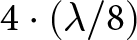 $4\cdot(\lambda/8)$, the difference between the reference and UAV-mounted configurations is typically 1–1.5 dB lower than at the closer positions. These results indicate that parasitic coupling and airframe-induced scattering remain limited under the investigated conditions. Consequently, field uniformity is not significantly degraded.
Based on these findings, the examined UAV can be considered suitable as an auxiliary platform for cellular-network EM exposure and performance measurements. This conclusion is supported by the fact that acceptable uncertainty levels in real-world measurements are typically higher than those observed under controlled laboratory conditions.
We emphasize that the results presented are specific to the investigated UAV platform, antenna type, mounting configuration, and controlled laboratory environment. Therefore, the findings cannot be directly generalized to other systems. The present study does not define a strict minimum separation of the antenna–airframe. Nevertheless, it is expected that the observed trends in the separation of the antenna-to-frame and the reduction of the perturbations induced by partially conductive CFRP structural elements with increasing spacing remain relevant for similar multirotor UAV configurations employing CF composite airframes. The results indicate that maintaining a separation greater than approximately half of the wavelength corresponding to the lowest frequency of interest is advisable, as this reduces the influence of the airframe on the measurement results.
In the next phase of the research, the investigations will be extended to address aspects not covered in the present work. In particular, the current study does not include Type-A (statistical) uncertainty evaluation or dynamic flight measurements. These factors may introduce additional variability under real operating conditions and will therefore require modified measurement procedures and dedicated data-processing approaches.
In addition, further investigation is required to assess the EM behavior of the UAV system more comprehensively. The onboard electronic subsystems, including brushless direct current (BLDC) motors, electronic speed controllers (ESCs), DC–DC converters, radio modules, and navigation units, may contribute to EM emissions that influence the measurements. The EM immunity of the UAV must also be evaluated, since external measurement equipment may interfere with flight-control and navigation systems. Moreover, during operation, the periodic occultation and scattering caused by the rotors (propellers) on the receive channel produce amplitude and phase modulation, which manifests as micro-Doppler sidebands and RPM-dependent (revolutions per minute) signal-level fluctuations, increasing Type-A uncertainty and potentially distorting the measurement results. Future work will address additional EM and operational aspects not covered in the present study, including the development of mathematical modeling and simulation-based analysis of UAV–antenna interactions. The present study focuses on the most widely used sub-6 GHz mobile communication bands. Future investigations will extend the analysis to higher frequency ranges, including millimeter-wave (mmWave) bands and other emerging frequency regimes, where additional validation will be required before extrapolating the present conclusions. At these frequency ranges, the reduced wavelength may further increase the sensitivity of the measurements to UAV airframe-induced perturbations. Therefore, subsequent research will focus on the following directions:
• Extension of the investigation to additional frequency bands (including mmWave and other emerging spectrum regimes)
• Cross-polarization measurements and airframe-induced cross-polarization discrimination (XPD) analysis
• EMC characterization, including emission and immunity
• Dynamic flight measurements, including rotor-induced scattering and time-varying channel effects
• Development of mathematical and simulation-based models for UAV–antenna interactions
• Evaluation of alternative UAV platforms, antenna types, and mounting configurations.
Competing interests
The authors declare no conflict of interest.
Appendix A. Averaged results
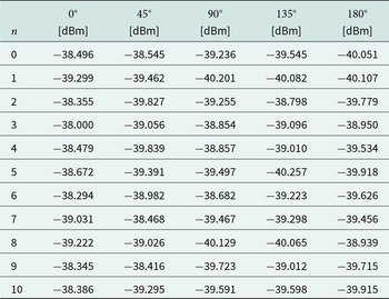
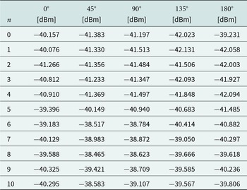
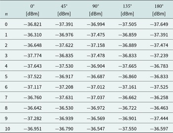
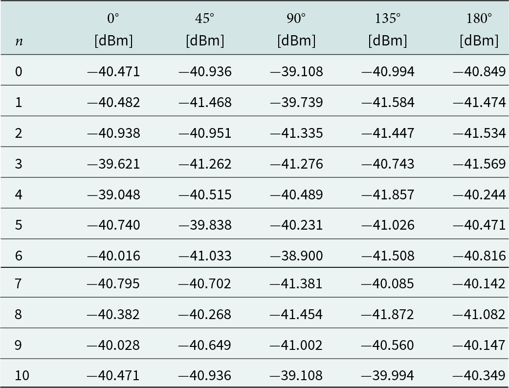
The data processing is based on time-averaged results obtained from both the reference and UAV-mounted configurations for each frequency, receive antenna height, and orientation. Tables A1–A14 present the averaged electromagnetic power level measurement results over the frequency range 700–3500 MHz.
700 MHz – averaged electromagnetic power levels – reference configuration

700 MHz – averaged electromagnetic power levels – UAV-mounted configuration

800 MHz – averaged electromagnetic power levels – reference configuration

800 MHz – averaged electromagnetic power levels – UAV-mounted configuration

900 MHz – averaged electromagnetic power levels – reference configuration

900 MHz – averaged electromagnetic power levels – UAV-mounted configuration

1800 MHz – averaged electromagnetic power levels – reference configuration

1800 MHz – averaged electromagnetic power levels – UAV-mounted configuration

2100 MHz – averaged electromagnetic power levels – reference configuration

2100 MHz – averaged electromagnetic power levels – UAV-mounted configuration

2600 MHz – averaged electromagnetic power levels – reference configuration

2600 MHz – averaged electromagnetic power levels – UAV-mounted configuration

3500 MHz – averaged electromagnetic power levels – reference configuration

3500 MHz – averaged electromagnetic power levels – UAV-mounted configuration

Appendix B. Abbreviations in alphabetical order
- BLDC
Brushless direct current
- CERP
Combined effective radiation pattern
- CF
Carbon-fiber
- CFRP
Carbon-fiber reinforced polymer
- DC
Direct current
- DGPS
Differential global positioning system
- EM
Electromagnetic
- EMC
Electromagnetic compatibility
- EMF
Electromagnetic field
- ESC
Electronic speed controller
- EUT
Equipment under test
- FAC
Fully anechoic chamber
- ICNIRP
International Commission on Non-Ionizing
Radiation Protection
- IEC
International Electrotechnical Commission
- ISM
Industrial, Scientific, and Medical
- mmWave
Millimeter-wave
- NR
New Radio – 5G
- RBW
Resolution bandwidth
- REM
Radio environment map
- RF
Radio frequency
- RF-EMF
Radio frequency electromagnetic field
- RMS
Root mean square
- RPM
Revolutions per minute
- RTK
Real-time kinematic
- SDR
Software defined radio
- SPA
Spectrum analyzer
- UAV
Unmanned aerial vehicle (drone)
- VBW
Video bandwidth
- VREM
Virtual radio environment map
- VSWR
Voltage standing wave ratio
- XPD
Cross-polarization discrimination














 Open access

