


1. Introduction
Many engineering and environmental systems involve the transport of heat or mass to finite active wall segments from flowing fluids. Examples include localised monolayer adsorption (Centres et al. Reference Centres, Bulnes, Riccardo, Ramirez-Pastor and Perarnau2011), reactive patches (Barzykin & Shushin Reference Barzykin and Shushin2001), porous systems (Bazaikin et al. Reference Bazaikin, Malkovich, Prokhorov and Derevschikov2021) and measurement of wall shear stress using electrochemical sensors (Havlica, Kramolis & Huchet Reference Havlica, Kramolis and Huchet2021). In these applications, the active segment of finite length is followed by an inactive surface, creating a wake region where the scalar field gradually recovers to ambient conditions. Despite the practical importance of understanding this wake behaviour for predicting interference between adjacent segments and optimising system performance, no analytical solution has been available for the scalar field in the wake region.
The theoretical foundation for convective heat and mass transfer near walls was established by Graetz (Reference Graetz1885), who derived the solution for heat transfer in tubes with fully developed laminar flow. This work was significantly extended by Lévêque (Reference Lévêque1928), who obtained a more practical solution by considering the thin boundary layer limit with a linear velocity profile near the wall. The Lévêque solution, expressing the local transfer rate in terms of the wall shear rate and distance from the leading edge, has become fundamental to understanding transport in laminar boundary layers. However, both the Graetz and Lévêque solutions provide no information about the wake region behind a finite active segment.
Subsequent research has extended these classical solutions in various directions. Apelblat (Reference Apelblat1982) analysed different velocity profiles beyond the linear approximation. Wang & Chang (Reference Wang and Chang2019) focused on non-Newtonian fluids with complex rheology. The effects of chemical reactions at active surfaces were considered by Pallares & Grau (Reference Pallares and Grau2014), whilst Haase et al. (Reference Haase, Chapman, Tsai, Lohse and Lammertink2015) extended the theory to flows with variable slip length at the wall. Bertsche et al. (Reference Bertsche, Meinicke, Knipper, Dubil and Wetzel2021) employed a generalised Lévêque equation relating heat transfer to pressure drop. However, all these extensions focussed exclusively on the zone above the segment.
Mass transport occurring in the region further downstream of the segment has received limited analytical treatment. Attempts to address finite active surfaces included numerical studies (Haase & Lammertink Reference Haase and Lammertink2016; Shah, Lin & Shaqfeh Reference Shah, Lin and Shaqfeh2017), but these do not provide closed-form analytical expressions for the wake region. The wake behind a finite sink represents a fundamental transport problem where the boundary condition changes from Dirichlet (fixed scalar value) to Neumann (zero flux), creating a mixed boundary value problem that has resisted analytical solution.
Beyond theoretical interest, understanding wake behaviour has practical implications across multiple fields. In electrochemical systems, the wake from upstream electrodes can interfere with downstream measurements, affecting sensor accuracy (Harrandt et al. Reference Harrandt, Kramolis, Huchet, Tihon and Havlica2023). In biological applications, the transport of nutrients or drugs from finite patches influences tissue growth and treatment efficacy (Caccavale et al. Reference Caccavale, De Bonis, Marino and Ruocco2020). Environmental applications include heat transfer in particle-laden gas flows (Kuruneru et al. Reference Kuruneru, Saha, Sauret and Gu2019), thermal erosion by lava flows (Kerr Reference Kerr2001) and heat transfer during bubble bursting (Poulain, Villermaux & Bourouiba Reference Poulain, Villermaux and Bourouiba2018). In all these cases, quantifying the wake extent and recovery rate is essential for system design and prediction.
This work presents the complete analytical solution for the laminar wake behind a finite wall-mounted sink. The approach employs Laplace transform methods to couple the classical Dirichlet problem over the active surface with the Neumann problem in the wake region. Through convolution-based integral relations, these two problems are unified into a single analytical framework. The resulting closed-form expression reduces to the Lévêque solution above the sink and provides a new analytical characterisation of the wake involving incomplete beta functions. The solution is validated through comparison with numerical simulations and analysed to extract characteristic wake lengths. This analytical framework fills a long-standing gap in boundary layer theory and provides a practical tool for designing systems with segmented active surfaces.
2. Problem formulation
We consider the steady convective–diffusive transport of a passive scalar $\phi$
(temperature or concentration) in a laminar boundary layer flow over a flat wall. The wall contains a finite segment of length
$\phi$
(temperature or concentration) in a laminar boundary layer flow over a flat wall. The wall contains a finite segment of length $L_{\!X}$
that acts as a sink for the scalar quantity, while the remaining wall surface is impermeable and inert. This configuration occurs in segmented heat exchangers, electrochemical sensors and environmental transport processes.
$L_{\!X}$
that acts as a sink for the scalar quantity, while the remaining wall surface is impermeable and inert. This configuration occurs in segmented heat exchangers, electrochemical sensors and environmental transport processes.
A Cartesian coordinate system $(X,Y,Z)$
is adopted with the wall located at
$(X,Y,Z)$
is adopted with the wall located at $Z = 0$
. The active sink segment spans
$Z = 0$
. The active sink segment spans $0 \lt X \leq L_{\!X}$
in the streamwise direction, the
$0 \lt X \leq L_{\!X}$
in the streamwise direction, the $Y$
axis extends in the spanwise direction and the
$Y$
axis extends in the spanwise direction and the $Z$
axis points into the fluid. The flow is unidirectional with velocity
$Z$
axis points into the fluid. The flow is unidirectional with velocity $\boldsymbol{u}(X,Z) = u(X,Z)\,\hat {\boldsymbol{e}}_{\!X}$
, where
$\boldsymbol{u}(X,Z) = u(X,Z)\,\hat {\boldsymbol{e}}_{\!X}$
, where $\hat {\boldsymbol{e}}_{\!X}$
denotes the unit vector in the streamwise direction. Figure 1 illustrates the problem geometry and the characteristic boundary layer thicknesses.
$\hat {\boldsymbol{e}}_{\!X}$
denotes the unit vector in the streamwise direction. Figure 1 illustrates the problem geometry and the characteristic boundary layer thicknesses.
Schematic of the flow configuration, showing the sink region, coordinate system and boundary-layer thicknesses: $\delta _{\!{H}}$
(hydrodynamic) and
$\delta _{\!{H}}$
(hydrodynamic) and $\delta _{\!{D}}$
(diffusive).
$\delta _{\!{D}}$
(diffusive).

The transport of the passive scalar is governed by the convection–diffusion equation
 \begin{align} \frac {\partial \phi }{\partial t} + \boldsymbol{u} \boldsymbol{\cdot }\boldsymbol{\nabla \!}\phi = D\kern-1pt \boldsymbol{\nabla} ^2 \phi , \end{align}
where $D$
denotes the molecular diffusivity (thermal diffusivity for heat transfer or mass diffusivity for species transport). The scalar is considered passive, implying it does not influence the velocity field.
$D$
denotes the molecular diffusivity (thermal diffusivity for heat transfer or mass diffusivity for species transport). The scalar is considered passive, implying it does not influence the velocity field.
To obtain an analytically tractable problem while retaining the essential physics, we adopt the following boundary-layer assumptions (Harrandt et al. Reference Harrandt, Bazaikin, Huchet, Tihon and Havlica2024).
-
(i) Steady state: $\partial \phi /\partial t = 0$
, as all boundary conditions and flow parameters are time-invariant.
$\partial \phi /\partial t = 0$
, as all boundary conditions and flow parameters are time-invariant. -
(ii) Linear velocity profile: within the viscous sublayer, the velocity profile is approximated by
(2.2)where
\begin{align} \boldsymbol{u}(Z) = S_{\!X}\! Z \hat {\boldsymbol{e}}_{\!X}, \end{align}
$S_{\!X}$
represents the constant wall shear rate. This approximation is valid when the scalar diffusion layer remains entirely within the viscous sublayer or laminar boundary layer, i.e.
$\delta _{\!{D}} \ll \delta _{\!{H}}$
.
-
(iii) Negligible streamwise diffusion: the streamwise diffusion term
$D\partial ^2\phi /\partial\! X^2$
is negligible compared with streamwise convection
$u \partial \phi /\partial\! X$
when the Péclet number based on sink length satisfies
$\textit{Pe}_{L_{\!X}} = S_{\!X} L_{\!X}^2 / D \gg 1$
. This condition ensures convection-dominated transport in the streamwise direction. -
(iv) Two-dimensional transport: variations in the spanwise direction (
$Y$
) are negligible. This assumption holds when the sink width in the
$Y$
-direction greatly exceeds the diffusion layer thickness, yielding
$\partial \phi / \partial Y \ll \partial \phi / \partial\! Z$
.


The validity of the linear velocity approximation can be assessed by examining characteristic length scales in the laminar boundary layer. For flow over a flat plate with kinematic viscosity $\nu$
and free stream velocity
$\nu$
and free stream velocity $U_\infty$
, the hydrodynamic boundary layer thickness and wall shear rate follow the Blasius scaling (Schlichting & Gersten Reference Schlichting and Gersten2017)
$U_\infty$
, the hydrodynamic boundary layer thickness and wall shear rate follow the Blasius scaling (Schlichting & Gersten Reference Schlichting and Gersten2017)
 \begin{align} \delta _{\!{H}} \sim \left ( \frac {\nu\! X}{U_\infty } \right )^{1/2}\!, \quad S_{\!X} \sim \frac {U_\infty }{\delta _{\!{H}}}, \end{align}
while the scalar diffusion layer thickness obeys the following scaling
 \begin{align} \delta _{\!{D}} \sim \left ( \frac {D\! X}{S_{\!X}} \right )^{1/3}\!. \end{align}
Combining these relations yields
 \begin{align} \frac {\delta _{\!{D}}}{\delta _{\!{H}}} \sim \textit{Sc}^{-1/3} \textit{Re}_X^{-1/6}, \end{align}
where $\textit{Sc} = \nu /\!D$
is the Schmidt number (or Prandtl number for heat transfer) and
$\textit{Sc} = \nu /\!D$
is the Schmidt number (or Prandtl number for heat transfer) and $\textit{Re}_X = U_\infty X / \nu$
is the local Reynolds number. For typical liquids with
$\textit{Re}_X = U_\infty X / \nu$
is the local Reynolds number. For typical liquids with $\textit{Sc} \gg 1$
and moderate to high Reynolds numbers, this ratio remains small, justifying the linear velocity approximation.
$\textit{Sc} \gg 1$
and moderate to high Reynolds numbers, this ratio remains small, justifying the linear velocity approximation.
At the sink trailing edge ( $X = L_{\!X}$
), assumption (iii) requires
$X = L_{\!X}$
), assumption (iii) requires
 \begin{align} \frac {\delta _{\!{D}}(L_{\!X})}{L_{\!X}} \sim \left ( \frac {D}{S_{\!X} L_{\!X}^2} \right )^{1/3} = \textit{Pe}_{L_{\!X}}^{-1/3}, \end{align}
which confirms that streamwise diffusion is negligible when $\textit{Pe}_{L_{\!X}} \gg 1$
.
$\textit{Pe}_{L_{\!X}} \gg 1$
.
Under these assumptions, (2.1) reduces to the boundary-layer form
 \begin{align} Z\! S_{\!X} \frac {\partial \phi }{\partial\! X} = D \frac {\partial ^2 \phi }{\partial\! Z^2}. \end{align}
Introducing the dimensionless variables,
 \begin{align} x = \sqrt {\frac {S_{\!X}}{D}}X, \quad z = \sqrt {\frac {S_{\!X}}{D}}Z, \end{align}
transforms the governing equation to the canonical form
 \begin{align} z \frac {\partial \phi }{\partial x} = \frac {\partial ^2 \phi }{\partial z^2}. \end{align}
The boundary conditions for this problem are
 \begin{align} \phi (0, z) &= \phi _\infty && \text{(inlet)}, \\[-12pt] \nonumber \end{align}
 \begin{align} \lim _{x^2 + z^2 \to \infty } \phi (x, z) &= \phi _\infty && \text{(far field)}, \\[-12pt] \nonumber \end{align}
 \begin{align} \phi (x, 0) &= \phi _{{w}} && 0 \lt x \leq L_{\kern-1pt x} \quad \text{(sink)}, \\[-12pt] \nonumber \end{align}
 \begin{align} \left . \frac {\partial \phi }{\partial z} \right |_{z=0} &= 0 && x \gt L_{\kern-1pt x} \quad \text{(inert wall)}, \\[9pt] \nonumber \end{align}
where $\phi _\infty$
represents the far-field scalar value,
$\phi _\infty$
represents the far-field scalar value, $\phi _{{w}}$
is the prescribed value at the sink surface and
$\phi _{{w}}$
is the prescribed value at the sink surface and $L_{\kern-1pt x} = \sqrt {S_{\!X} / D} L_{\!X}$
is the dimensionless sink length.
$L_{\kern-1pt x} = \sqrt {S_{\!X} / D} L_{\!X}$
is the dimensionless sink length.
The boundary condition exhibits a discontinuity at $x = L_{\kern-1pt x}$
, where the Dirichlet condition transitions to a Neumann condition. Despite this discontinuity, the problem remains mathematically well-posed due to the parabolic nature of (2.9) and the uniform inlet condition. The solution strategy, presented in the following section, addresses this transition by solving coupled subproblems for the regions above and downstream of the sink.
$x = L_{\kern-1pt x}$
, where the Dirichlet condition transitions to a Neumann condition. Despite this discontinuity, the problem remains mathematically well-posed due to the parabolic nature of (2.9) and the uniform inlet condition. The solution strategy, presented in the following section, addresses this transition by solving coupled subproblems for the regions above and downstream of the sink.
3. Analytical solution
This section presents the analytical solution for the scalar field $\phi$
in the region above and beyond the finite sink. The solution strategy employs Laplace transform methods to solve the governing equation (2.9) subject to the boundary conditions (2.10). The key innovation lies in coupling the Dirichlet problem (above the sink) with the Neumann problem (in the wake) through a system of integral relations.
$\phi$
in the region above and beyond the finite sink. The solution strategy employs Laplace transform methods to solve the governing equation (2.9) subject to the boundary conditions (2.10). The key innovation lies in coupling the Dirichlet problem (above the sink) with the Neumann problem (in the wake) through a system of integral relations.
3.1. General solution via Laplace transform
To facilitate the analysis, we first introduce a shifted scalar field that satisfies homogeneous far-field conditions,
 \begin{align} \phi ^* = \phi - \phi _\infty , \end{align}
which transforms the governing equation (2.9) to
 \begin{align} z \frac {\partial \phi ^*}{\partial x} = \frac {\partial ^2 \phi ^*}{\partial z^2} . \end{align}
The boundary conditions become
 \begin{align} \phi ^*(0, z) &= 0 && \text{(inlet)}, \\[-12pt] \nonumber \end{align}
 \begin{align} \lim _{x^2 + z^2 \to \infty } \phi ^*(x, z) &= 0 && \text{(far field)}, \\[-12pt] \nonumber \end{align}
 \begin{align} \phi ^*(x, 0) &= \phi _{{w}} - \phi _\infty, && 0 \lt x \leq L_{\kern-1pt x} \quad \text{(sink)}, \\[-12pt] \nonumber \end{align}
 \begin{align} \left . \frac {\partial \phi ^*}{\partial z} \right |_{z=0} &= 0, && x \gt L_{\kern-1pt x} \quad \text{(inert wall)}. \\[9pt] \nonumber \end{align}
We define two auxiliary functions that characterise the wall behaviour
 \begin{align} \varPi (x) &= \phi ^*(x, 0) , \\[-12pt] \nonumber\end{align}
 \begin{align} \varPsi (x) &= \left . \frac {\partial \phi ^*(x, z)}{\partial z} \right |_{z=0}\! . \\[9pt] \nonumber \end{align}
These represent the scalar value and its wall-normal gradient along the wall, respectively.
The Laplace transform with respect to the streamwise coordinate $x$
is defined as
$x$
is defined as
 \begin{align} \varPhi ^*(s, z) = \mathcal{L} \{ \phi ^*(x, z) \}(s) = \int _0^\infty {e}^{-s x} \phi ^*(x, z) \, {\rm d}x , \end{align}
where $s$
is a complex variable with
$s$
is a complex variable with $\mathrm{Re}(s) \gt 0$
. Applying the Laplace transform to (3.2) and using the derivative property (Lipschutz, Spiegel & Liu Reference Lipschutz, Spiegel and Liu2009)
$\mathrm{Re}(s) \gt 0$
. Applying the Laplace transform to (3.2) and using the derivative property (Lipschutz, Spiegel & Liu Reference Lipschutz, Spiegel and Liu2009)
 \begin{align} \mathcal{L} \left\{ \frac {\partial \phi ^*}{\partial x} \right\}(s) = s \mathcal{L} \{ \phi ^* \}(s) - \phi ^*(0^{-}, z) , \end{align}
together with the inlet condition $\phi ^*(0^{-}, z) = 0$
, yields the transformed equation
$\phi ^*(0^{-}, z) = 0$
, yields the transformed equation
 \begin{align} \textit{sz} \varPhi ^*(s, z) = \frac {\partial ^2 \varPhi ^*(s, z)}{\partial z^2} . \end{align}
This is the Airy differential equation, whose general solution is (Vallée & Soares Reference Vallée and Soares2010)
 \begin{align} \varPhi ^*(s, z) = \frac {\alpha (s)}{{\mathrm{Ai}}(0) s} {\mathrm{Ai}}\big(s^{1/3} z \big) + \beta (s) {\mathrm{Bi}}\big(s^{1/3} z \big) , \end{align}
where $\mathrm{Ai}$
and
$\mathrm{Ai}$
and $\mathrm{Bi}$
are the Airy functions of the first and second kind, respectively. The prefactor
$\mathrm{Bi}$
are the Airy functions of the first and second kind, respectively. The prefactor $1/({\mathrm{Ai}}(0)s)$
is introduced for clarity in later algebraic manipulation. We define
$1/({\mathrm{Ai}}(0)s)$
is introduced for clarity in later algebraic manipulation. We define $s^{1/3}$
as the principal value of the complex cube root, taken on the branch containing the positive real semi-axis (
$s^{1/3}$
as the principal value of the complex cube root, taken on the branch containing the positive real semi-axis ( $s \gt 0$
).
$s \gt 0$
).
Since $\mathrm{Bi}(z) \to \infty$
as
$\mathrm{Bi}(z) \to \infty$
as $z \to \infty$
(Vallée & Soares Reference Vallée and Soares2010), the far-field condition (3.3b
) requires
$z \to \infty$
(Vallée & Soares Reference Vallée and Soares2010), the far-field condition (3.3b
) requires $\beta (s) = 0$
. Thus,
$\beta (s) = 0$
. Thus,
 \begin{align} \varPhi ^*(s, z) = \frac {\alpha (s)}{{\mathrm{Ai}}(0) s} \mathrm{Ai}\big(s^{1/3} z \big) . \end{align}
Here, $\alpha (s)$
is an undetermined function that will be fixed by the boundary conditions; it is unique for the mixed boundary-value problem and depends on the wall traces of the solution.
$\alpha (s)$
is an undetermined function that will be fixed by the boundary conditions; it is unique for the mixed boundary-value problem and depends on the wall traces of the solution.
For $s \gt 0$
, the Airy function admits the integral representation (Reid Reference Reid1995)
$s \gt 0$
, the Airy function admits the integral representation (Reid Reference Reid1995)
 \begin{align} \frac {1}{s} \mathrm{Ai}\big(s^{1/3} z \big) = \frac {\sqrt {3}}{2 \pi s} \int _0^\infty \exp\! \left ( - \frac {s z^3 t^3}{3} - \frac {1}{3 t^3} \right ) \frac {1}{t^2} \, {\rm d}t . \end{align}
Changing variables using $u = 1/(3^{1/3} t)$
gives
$u = 1/(3^{1/3} t)$
gives
 \begin{align} \frac {1}{s} \mathrm{Ai}\big(s^{1/3} z \big) = \frac {3^{5/6}}{2 \pi s} \int _0^\infty \exp\! \left ( - \frac {s z^3}{9 u^3} - u^3 \right ) \, {\rm d}u . \end{align}
We can rewrite the integrand in the following way
 \begin{align} \frac {1}{s} \mathrm{Ai}\big(s^{1/3} z \big) = \frac {3^{5/6}}{2 \pi } \int _0^\infty {\mathrm{e}}^{-u^3} \left ( \frac {1}{s} {\mathrm{e}}^{- \frac {s z^3}{9 u^3}} \right ) \, {\rm d}u . \end{align}
Recognising the inner exponential as a Laplace kernel, we write
 \begin{align} \frac {1}{s} {\mathrm{e}}^{- \frac {s z^3}{9 u^3}} = \int _{z^3/(9 u^3)}^\infty {\mathrm{e}}^{-s x} \, {\rm d}x . \end{align}
Reversing the order of integration leads to the double integral
 \begin{align} \frac {1}{s} {\mathrm{Ai}}\big(s^{1/3} z \big) = \frac {3^{5/6}}{2 \pi } \int _0^\infty {\mathrm{e}}^{-s x} \left ( \int _{z (9x)^{-1/3}}^\infty {\mathrm{e}}^{-u^3} \, {\rm d}u \right ) {\rm d}x . \end{align}
Thus, we express the Airy function as a Laplace transform,
 \begin{align} \frac {1}{s} \mathrm{Ai}\big(s^{1/3} z \big) = \frac {3^{5/6}}{2 \pi } \mathcal{L}\! \left \{ \int _{z (9x)^{-1/3}}^\infty {\mathrm{e}}^{-u^3} \, {\rm d}u \right \}(s) . \end{align}
Substituting into (3.9), we find
 \begin{align} \varPhi ^*(s, z) = \frac {\alpha (s)}{{\mathrm{Ai}}(0)} \frac {3^{5/6}}{2 \pi } \mathcal{L}\! \left \{ \int _{z (9x)^{-1/3}}^\infty {\mathrm{e}}^{-u^3} \, {\rm d}u \right \}(s) . \end{align}
Using the identity (Abramowitz Reference Abramowitz1974)
 \begin{align} \mathrm{Ai}(0) = \frac {1}{3^{2/3} \varGamma (2/3)} \, \end{align}
and the gamma function identity $\varGamma (2/3) \varGamma (4/3) = 2 \pi / (3\sqrt {3})$
, the prefactor simplifies to
$\varGamma (2/3) \varGamma (4/3) = 2 \pi / (3\sqrt {3})$
, the prefactor simplifies to
 \begin{align} \frac {3 \sqrt {3} \varGamma (2/3)}{2 \pi } = \frac {1}{\varGamma (4/3)} . \end{align}
Hence, we obtain the final general form of the Laplace-transformed scalar field
 \begin{align} \varPhi ^*(s, z) = \frac {\alpha (s)}{\varGamma (4/3)} \mathcal{L}\! \left \{ \int _{z (9x)^{-1/3}}^\infty {\mathrm{e}}^{-u^3} \, {\rm d}u \right \}(s) . \end{align}
In the following derivations, the product of two Laplace transforms will appear. To evaluate the inverse transform of such expressions, we apply the Laplace convolution theorem. For this purpose, we recall the standard definition of convolution, which will be used in the subsequent subsections. The convolution of two functions $f(x)$
and
$f(x)$
and $g(x)$
is defined as
$g(x)$
is defined as
 \begin{align} (f * g)(x) = \int _0^x\! f(\xi )\, g(x - \xi )\, {\rm d}\xi , \end{align}
where $*$
denotes the convolution operator. This identity is particularly useful when expressing inverse Laplace transforms of products of individual transforms.
$*$
denotes the convolution operator. This identity is particularly useful when expressing inverse Laplace transforms of products of individual transforms.
3.2. Solution of the Dirichlet problem
For the region above the sink $(0 \lt x \leq L_{\kern-1pt x})$
, the Dirichlet boundary condition (3.3c
) applies. From the general solution (3.9), we evaluate the scalar field at the wall, where
$(0 \lt x \leq L_{\kern-1pt x})$
, the Dirichlet boundary condition (3.3c
) applies. From the general solution (3.9), we evaluate the scalar field at the wall, where $z = 0$
, to obtain
$z = 0$
, to obtain
 \begin{align} \varPhi ^*(s, 0) = \frac {\alpha (s)}{s} . \end{align}
Using the definition of the auxiliary function $\varPi (x)$
from (3.4a
), and the Laplace transform (3.5), we write
$\varPi (x)$
from (3.4a
), and the Laplace transform (3.5), we write
 \begin{align} \frac {\alpha (s)}{s} = \mathcal{L}\! \left \{ \varPi (x) \right \}(s) . \end{align}
Solving for $\alpha (s)$
and applying the Laplace identity for derivatives (Lipschutz et al. Reference Lipschutz, Spiegel and Liu2009)
$\alpha (s)$
and applying the Laplace identity for derivatives (Lipschutz et al. Reference Lipschutz, Spiegel and Liu2009)
 \begin{align} \mathcal{L} \{ \varPi '(x) \}(s) = s \mathcal{L}\! \left \{ \varPi (x) \right \}(s) - \varPi (0^-) , \end{align}
we obtain
 \begin{align} \alpha (s) = \mathcal{L} \{ \varPi '(x) \}(s) , \end{align}
where we have used the fact that $\varPi (0^-) = 0$
.
$\varPi (0^-) = 0$
.
Substituting this result into (3.19) yields the Laplace image of the scalar field,
 \begin{align} \varPhi ^*(s, z) = \frac {1}{\varGamma (4/3)} \mathcal{L} \{ \varPi '(x) \}(s) \mathcal{L}\! \left \{ \int _{z (9x)^{-1/3}}^\infty {\mathrm{e}}^{-u^3} \, {\rm d}u \right \}(s) . \end{align}
Using the convolution theorem for Laplace transforms (Doetsch Reference Doetsch1974) and the definition of convolution given in (3.20), this becomes
 \begin{align} \varPhi ^*(s, z) = \frac {1}{\varGamma (4/3)} \mathcal{L}\! \left \{ \varPi '(x) * \int _{z (9x)^{-1/3}}^\infty {\mathrm{e}}^{-u^3} \, {\rm d}u \right \}(s) . \end{align}
Applying the inverse Laplace transform, we obtain the scalar field in the physical domain,
 \begin{align} \phi ^*(x, z) = \frac {1}{\varGamma (4/3)} \int _0^x \varPi '(\xi )\! \left ( \int _{z (9(x - \xi ))^{-1/3}}^\infty {\mathrm{e}}^{-u^3} \, {\rm d}u \right ) {\rm d}\xi . \end{align}
Using Fubini’s theorem, the order of integration in (3.27) can be reversed. Further expressing the upper limit of the current inner integral from the relation $u = z (9(x - \xi ))^{-1/3}$
, the expression becomes
$u = z (9(x - \xi ))^{-1/3}$
, the expression becomes
 \begin{align} \int _{z (9x)^{-1/3}}^\infty\! \left ( \int _0^{x - \frac {z^3}{9u^3}} \varPi '(\xi ) \, {\rm d}\xi \right ) {\mathrm{e}}^{-u^3} \, {\rm d}u . \end{align}
Evaluating the inner integral gives
 \begin{align} \int _{z (9x)^{-1/3}}^\infty \left [ \varPi\! \left ( x - \frac {z^3}{9u^3} \right ) - \varPi (0) \right ] {\mathrm{e}}^{-u^3} \, {\rm d}u . \end{align}
Since $\varPi (0) = 0$
, we obtain the final result for the Dirichlet case
$\varPi (0) = 0$
, we obtain the final result for the Dirichlet case
 \begin{align} \phi ^*(x, z) = \frac {1}{\varGamma (4/3)} \int _{z (9x)^{-1/3}}^\infty \varPi\! \left ( x - \frac {z^3}{9u^3} \right ) {\mathrm{e}}^{-u^3} \, {\rm d}u . \end{align}
3.3. Solution of the Neumann problem
We now consider the general solution (3.9) in the case where the Neumann boundary condition (3.3d
) is imposed. Evaluating the derivative of (3.9) with respect to the variable $z$
, we obtain
$z$
, we obtain
 \begin{align} \frac {\partial \varPhi ^{*}(s, 0)}{\partial z} = \frac {\alpha (s)}{{\mathrm{Ai}}(0) s^{2/3}} {\mathrm{Ai}}'(0) . \end{align}
Using (3.4b ) together with the Laplace transform (3.5), this relation can be written as
 \begin{align} \frac {\alpha (s)}{{\mathrm{Ai}}(0) s^{2/3}} \mathrm{Ai}'(0) = \mathcal{L}\! \left \{ \varPsi (x) \right \}(s) . \end{align}
Isolating the function $\alpha (s)$
from (3.32) yields
$\alpha (s)$
from (3.32) yields
 \begin{align} \alpha (s)=\frac {{\mathrm{Ai}}(0)\,s^{2/3}}{\mathrm{Ai}'(0)}\,\mathcal{L}\{\varPsi (x)\}(s). \end{align}
To express this in terms of $\mathcal{L}\{\varPsi '(x)\}(s)$
, we use the Laplace transform identity for derivatives with respect to
$\mathcal{L}\{\varPsi '(x)\}(s)$
, we use the Laplace transform identity for derivatives with respect to $x$
,
$x$
,
 \begin{align} s\,\mathcal{L}\{\varPsi (x)\}(s)=\mathcal{L}\{\varPsi '(x)\}(s)+\varPsi (0^-). \end{align}
Since the inlet condition $\phi ^*(0,z)=0$
implies
$\phi ^*(0,z)=0$
implies $\partial _z\phi ^*(0,z)=0$
, we have
$\partial _z\phi ^*(0,z)=0$
, we have $\varPsi (0^-)=0$
and hence
$\varPsi (0^-)=0$
and hence $\mathcal{L}\{\varPsi (x)\}(s)=s^{-1}\mathcal{L}\{\varPsi '(x)\}(s)$
. Substituting this relation into the expression for
$\mathcal{L}\{\varPsi (x)\}(s)=s^{-1}\mathcal{L}\{\varPsi '(x)\}(s)$
. Substituting this relation into the expression for $\alpha (s)$
and simplifying yields
$\alpha (s)$
and simplifying yields
 \begin{align} \alpha (s) = \frac {{\mathrm{Ai}}(0)}{{\mathrm{Ai}}'(0) s^{1/3}} \mathcal{L} \{ \varPsi '(x) \}(s) . \end{align}
To evaluate the Laplace transform of the power functions appearing in the subsequent derivations, we recall the general identity (Abramowitz Reference Abramowitz1974)
 \begin{align} \mathcal{L}\!\left \{H(x)x^{k-1}\right \}(s)=\frac {\varGamma (k)}{s^k}, \qquad \mathrm{Re}(k)\gt 0, \end{align}
where $H(x)$
denotes the Heaviside function,
$H(x)$
denotes the Heaviside function,
 \begin{align} H(x)= \begin{cases} 0, & x\lt 0,\\ 1, & x\ge 0, \end{cases} \end{align}
which will be used later for specific values of $k$
to express the Laplace images of power functions. Equation (3.35) can now be written as
$k$
to express the Laplace images of power functions. Equation (3.35) can now be written as
 \begin{align} \alpha (s) = \frac {{\mathrm{Ai}}(0)}{{\mathrm{Ai}}'(0)} \frac {1}{\varGamma (1/3)} \mathcal{L} \{ x^{-2/3} \}(s) \mathcal{L} \{ \varPsi '(x) \}(s) . \end{align}
The general identity (3.36) is here applied with $k=1/3$
to evaluate the Laplace transform
$k=1/3$
to evaluate the Laplace transform $\mathcal{L}\{x^{-2/3}\}(s)$
appearing in (3.38).
$\mathcal{L}\{x^{-2/3}\}(s)$
appearing in (3.38).
The derivative of the Airy function of the first kind at the origin is given by (Vallée & Soares Reference Vallée and Soares2010)
 \begin{align} \mathrm{Ai}'(0) = -\frac {1}{3^{1/3} \varGamma (1/3)} . \end{align}
Substituting into the previous expression and recognising that the product of Laplace images corresponds to the Laplace transform of a convolution, we obtain
 \begin{align} \alpha (s) = -3^{1/3} \mathrm{Ai}(0) \, \mathcal{L} \big \{ x^{-2/3} * \varPsi '(x) \big \}(s) , \end{align}
where $*$
denotes convolution as defined in (3.20).
$*$
denotes convolution as defined in (3.20).
Substituting this form of $\alpha (s)$
into the general solution (3.19) yields
$\alpha (s)$
into the general solution (3.19) yields
 \begin{align} \varPhi ^{*}(s, z) = -\frac {3^{1/3} \mathrm{Ai}(0)}{\varGamma (4/3)} \mathcal{L} \big \{ x^{-2/3} * \varPsi '(x) \big \}(s) \mathcal{L}\! \left \{ \int _{z (9x)^{-1/3}}^\infty {\mathrm{e}}^{-u^3} \, {\rm d}u \right \}(s) . \end{align}
Applying the identities (3.17) and (3.18), the prefactor simplifies to
 \begin{align} \varPhi ^{*}(s, z) = -\frac {3^{7/6}}{2 \pi } \mathcal{L} \big \{ x^{-2/3} * \varPsi '(x) \big \}(s) \mathcal{L}\! \left \{ \int _{z (9x)^{-1/3}}^\infty {\mathrm{e}}^{-u^3} \, {\rm d}u \right \}(s) . \end{align}
Using the convolution identity in reverse, we now return to the physical domain. The product of Laplace images corresponds to a convolution in physical space, giving
 \begin{align} \phi ^{*}(x, z) = -\frac {3^{7/6}}{2 \pi }\! \int _0^x \big ( x^{-2/3} * \varPsi '(x) \big )\Big |_{x = \xi } \left ( \int _{z (9(x - \xi ))^{-1/3}}^\infty {\mathrm{e}}^{-u^3} \, {\rm d}u \right ) {\rm d}\xi . \end{align}
Substituting the definition of the convolution (3.20), we obtain the final expression for the scalar field in the Neumann case,
 \begin{align} \phi ^{*}(x, z) = -\frac {3^{7/6}}{2 \pi }\! \int _0^x \left ( \int _0^\xi \frac {\varPsi '(\chi )}{(\xi - \chi )^{2/3}} \, {\rm d}\chi \right ) \left ( \int _{z (9(x - \xi ))^{-1/3}}^\infty {\mathrm{e}}^{-u^3} \, {\rm d}u \right ) {\rm d}\xi .\\[-12pt]\nonumber \end{align}
3.4. Coupling relations between the two regions
In the domain of $\varPhi ^{*}(s, z)$
, the function
$\varPhi ^{*}(s, z)$
, the function $\alpha (s)$
appearing in the general solution can be expressed in two equivalent ways depending on which boundary condition is applied. From the Dirichlet boundary condition (3.24), we have
$\alpha (s)$
appearing in the general solution can be expressed in two equivalent ways depending on which boundary condition is applied. From the Dirichlet boundary condition (3.24), we have $\alpha (s) = \mathcal{L}\{\varPi '(x)\}$
, while from the Neumann boundary condition (3.32),
$\alpha (s) = \mathcal{L}\{\varPi '(x)\}$
, while from the Neumann boundary condition (3.32), $\alpha (s)$
can be expressed in terms of
$\alpha (s)$
can be expressed in terms of $\mathcal{L}\{\varPsi (x)\}$
. Since both expressions describe the same function
$\mathcal{L}\{\varPsi (x)\}$
. Since both expressions describe the same function $\alpha (s)$
in the same general solution, equating them yields the coupling relation between
$\alpha (s)$
in the same general solution, equating them yields the coupling relation between $\varPi '$
and
$\varPi '$
and $\varPsi$
,
$\varPsi$
,
 \begin{align} \mathcal{L} \{ \varPi '(x) \}(s) = \frac {{\mathrm{Ai}}(0)}{{\mathrm{Ai}}'(0)} s^{2/3} \mathcal{L}\! \left \{ \varPsi (x) \right \}(s) . \end{align}
By substituting from (3.17) and (3.39), this becomes
 \begin{align} \mathcal{L} \{ \varPi '(x) \}(s) = -\frac {\varGamma (1/3)}{3^{1/3} \varGamma (2/3)} s^{2/3} \mathcal{L}\! \left \{ \varPsi (x) \right \}(s) . \end{align}
Based on (3.46), we now derive mutual relations between the functions $\varPi$
and
$\varPi$
and $\varPsi$
in the domain of the transformed variable
$\varPsi$
in the domain of the transformed variable $\varPhi ^*(s, z)$
. The Laplace image of
$\varPhi ^*(s, z)$
. The Laplace image of $\varPsi$
can be written explicitly as
$\varPsi$
can be written explicitly as
 \begin{align} \mathcal{L}\! \left \{ \varPsi (x) \right \}(s) = -\frac {3^{1/3} \varGamma (2/3)}{\varGamma (1/3) s^{2/3}} \mathcal{L} \{ \varPi '(x) \}(s) . \end{align}
The term $\varGamma (2/3) s^{-2/3}$
corresponds to the Laplace transform of a power function for
$\varGamma (2/3) s^{-2/3}$
corresponds to the Laplace transform of a power function for $k=2/3$
according to (3.36),
$k=2/3$
according to (3.36),
 \begin{align} \frac {\varGamma (2/3)}{s^{2/3}} = \mathcal{L}\! \left \{ \frac {H(x)}{x^{1/3}} \right \}(s) . \end{align}
Substituting (3.48) into (3.47), we obtain
 \begin{align} \mathcal{L}\! \left \{ \varPsi (x) \right \}(s) = -\frac {3^{1/3}}{\varGamma (1/3)} \mathcal{L}\! \left \{ \frac {H(x)}{x^{1/3}} \right \}(s) \mathcal{L} \{ \varPi '(x) \}(s) . \end{align}
The Laplace image of the derivative $\varPi '$
can be expressed using the identity (3.6) as
$\varPi '$
can be expressed using the identity (3.6) as
 \begin{align} \mathcal{L} \{ \varPi '(x) \}(s) = s \mathcal{L}\! \left \{ \varPi (x) \right \}(s) - \varPi (0^-) = s \mathcal{L}\! \left \{ \varPi (x) \right \}(s) , \end{align}
where we again used the fact that $\varPi (0^-) = 0$
.
$\varPi (0^-) = 0$
.
Substituting (3.50) into (3.46), we find
 \begin{align} \mathcal{L}\! \left \{ \varPi (x) \right \}(s) = -\frac {\varGamma (1/3)}{3^{1/3} \varGamma (2/3) s^{1/3}} \mathcal{L}\! \left \{ \varPsi (x) \right \}(s) , \end{align}
which can be rearranged, again using (3.36) for $k=1/3$
, as
$k=1/3$
, as
 \begin{align} \mathcal{L}\! \left \{ \varPi (x) \right \}(s) = -\frac {1}{3^{1/3} \varGamma (2/3)} \mathcal{L}\! \left \{ \frac {H(x)}{x^{2/3}} \right \}(s) \mathcal{L}\! \left \{ \varPsi (x) \right \}(s) . \end{align}
Returning to the physical domain, we use (3.52) and (3.49) to write the final mutual relations between $\varPi$
and
$\varPi$
and $\varPsi$
. These are given by the following integral expressions
$\varPsi$
. These are given by the following integral expressions
 \begin{align} \varPi (x) = -\frac {1}{3^{1/3} \varGamma (2/3)} \int _0^x \frac {\varPsi (\chi )}{(x - \chi )^{2/3}} \, {\rm d}\chi , \end{align}
 \begin{align} \varPsi (x) = -\frac {3^{1/3}}{\varGamma (1/3)} \int _0^x \frac {\varPi '(\xi )}{(x - \xi )^{1/3}} \, {\rm d}\xi . \end{align}
These two integral expressions form a consistent mathematical coupling between the Dirichlet and Neumann wall functions and confirm the analytical compatibility of the respective subproblem solutions.
3.5. Complete solution for the scalar field
In this section, we derive the scalar field $\phi (x,z)$
both above the active sink and in the downstream wake region. The analysis begins with the Dirichlet solution over the sink, followed by an analytical continuation into the wake using the relation between
$\phi (x,z)$
both above the active sink and in the downstream wake region. The analysis begins with the Dirichlet solution over the sink, followed by an analytical continuation into the wake using the relation between $\varPi (x)$
and
$\varPi (x)$
and $\varPsi (x)$
established in § 3.4.
$\varPsi (x)$
established in § 3.4.
The scalar field above the sink is obtained by substituting the Dirichlet condition (3.3c
) into the integral solution (3.30), with $\varPi (x) = \phi _{{w}} - \phi _{\infty }$
. This yields
$\varPi (x) = \phi _{{w}} - \phi _{\infty }$
. This yields
 \begin{align} \phi ^*(x,z) = \frac {\phi _{{w}} - \phi _{\infty }}{\varGamma\! \left (\frac {4}{3}\right )} \int _{z(9x)^{-1/3}}^\infty {\mathrm{e}}^{-u^3} \, {\rm d}u \quad {\rm for} \quad x\in ( 0;L_{x}\rangle , \end{align}
and using (3.1), the original scalar field becomes
 \begin{align} \phi (x,z) = \phi _{\infty } + \frac {\phi _{{w}} - \phi _{\infty }}{\varGamma\! \left (\frac {4}{3}\right )} \int _{z(9x)^{-1/3}}^\infty {\mathrm{e}}^{-u^3} \, {\rm d}u \quad {\rm for} \quad x\in ( 0;L_{x}\rangle . \end{align}
This result is consistent with the classical Lévêque solution for forced convection from an isothermal flat plate (Lévêque Reference Lévêque1928). The previous expression can be rewritten in terms of the incomplete gamma function, which gives it a particularly simple form,
 \begin{align} \phi (x,z) = \phi _{\infty } + (\phi _{{w}} - \phi _{\infty }) \frac {\varGamma\! \left (\frac {1}{3}, \frac {z^3}{9x}\right )}{\varGamma\! \left (\frac {1}{3}\right )} \quad {\rm for} \quad x\in ( 0;L_{x}\rangle . \end{align}
To obtain the wake behaviour, we express the wall-normal derivative of $\phi ^*$
,
$\phi ^*$
,
 \begin{align} \varPsi (x) = \left . \frac {\partial \phi ^*(x,z)}{\partial z} \right |_{z=0} = \frac {\partial }{\partial z}\! \left ( \frac {\phi _{{w}} - \phi _{\infty }}{\varGamma\! \left(\frac {4}{3}\right)} \int _{z(9x)^{-1/3}}^\infty {\mathrm{e}}^{-u^3} \, {\rm d}u \right ) \bigg |_{z=0}, \end{align}
and applying Leibniz’s rule for the derivative of an integral with a lower limit containing $z$
, we find
$z$
, we find
 \begin{align} \varPsi (x) = \frac {\phi _{\infty } - \phi _{{w}}}{\varGamma\! \left (\frac {4}{3}\right )(9x)^{1/3}} \quad {\rm for} \quad x\in ( 0;L_{x}\rangle . \end{align}
Using the identity $\varGamma ({4}/{3}) = {1}/{3} \varGamma ( {1}/{3})$
, (3.59) takes the form
$\varGamma ({4}/{3}) = {1}/{3} \varGamma ( {1}/{3})$
, (3.59) takes the form
 \begin{align} \varPsi (x) = (\phi _{\infty } - \phi _{{w}}) \frac {3^{1/3}}{\varGamma\! \left(\frac {1}{3}\right)} \frac {1}{x^{1/3}} \quad \mathrm{for} \quad x\in ( 0;L_{x}\rangle . \end{align}
To generalise this expression for all $x \gt 0$
, including the inert wall region, we introduce the Heaviside function
$x \gt 0$
, including the inert wall region, we introduce the Heaviside function $H(L_{\kern-1pt x} - x)$
to enforce the Neumann boundary condition (3.3d
),
$H(L_{\kern-1pt x} - x)$
to enforce the Neumann boundary condition (3.3d
),
 \begin{align} \varPsi (x) = (\phi _{\infty } - \phi _{{w}}) \frac {3^{1/3}}{\varGamma\! \left(\frac {1}{3}\right)} \frac {1}{x^{1/3}} H(L_{\kern-1pt x} - x) \quad {\rm for} \quad x\gt 0 . \end{align}
Substituting (3.61) into the convolution relation (3.53), we obtain for $x \gt L_{\kern-1pt x}$
,
$x \gt L_{\kern-1pt x}$
,
 \begin{align} \varPi (x) = -\frac {\phi _{\infty } - \phi _{{w}}}{\varGamma\! \left(\frac {2}{3}\right) \varGamma\! \left(\frac {1}{3}\right)} \int _0^x \frac {H(L_{\kern-1pt x} - \chi )}{\chi ^{1/3}(x - \chi )^{2/3}} \, {\rm d}\chi . \end{align}
Replacing the gamma functions with the complete beta function $B({1}/{3}, {2}/{3})$
and removing the Heaviside function by changing the upper limit to
$B({1}/{3}, {2}/{3})$
and removing the Heaviside function by changing the upper limit to $L_{\kern-1pt x}$
, we write
$L_{\kern-1pt x}$
, we write
 \begin{align} \varPi (x) = -\frac {\phi _{\infty } - \phi _{{w}}}{B\!\left(\frac {1}{3}, \frac {2}{3}\right)} \int _0^{L_{\kern-1pt x}} \frac {1}{\chi ^{1/3}(x - \chi )^{2/3}} \, {\rm d}\chi . \end{align}
Using the change of variables $\zeta = \chi /x$
, we find
$\zeta = \chi /x$
, we find
 \begin{align} \varPi (x) = -\frac {\phi _{\infty } - \phi _{{w}}}{B\! \left(\frac {1}{3}, \frac {2}{3}\right)} \int _0^{L_{\kern-1pt x}/x} \frac {1}{\zeta ^{1/3}(1 - \zeta )^{2/3}} \, {\rm d}\zeta , \end{align}
and by further change of variables $\psi = 1 - \zeta$
, this becomes
$\psi = 1 - \zeta$
, this becomes
 \begin{align} \varPi (x) = \frac {\phi _{\infty } - \phi _{{w}}}{B\! \left(\frac {1}{3}, \frac {2}{3}\right)} \int _{1}^{1- L_{\kern-1pt x}/x} \frac {1}{(1 - \psi )^{1/3} \psi ^{2/3}} \, {\rm d}\psi . \end{align}
Then,
 \begin{align} \varPi (x) =\frac {\phi _{\infty }-\phi _{{w}}}{B\! \left(\frac {1}{3},\frac {2}{3}\right)}\! \left ( \int _{0}^{1-L_{x}/x} \frac {1}{(1 - \psi )^{1/3} \psi ^{2/3}}{\rm d}\psi - \int _{0}^{1} \frac {1}{(1 - \psi )^{1/3} \psi ^{2/3}}{\rm d}\psi \right )\! . \end{align}
To express this in terms of the complete and incomplete beta functions, we introduce its standard definition (Abramowitz Reference Abramowitz1974),
 \begin{align} B(x;\! \alpha ,\! \beta ) = \int _0^x \psi ^{\alpha - 1} (1 - \psi )^{\beta - 1} \, {\rm d}\psi , \end{align}
and note that the complete beta function satisfies $B(\alpha ,\beta )=B(1;\alpha ,\beta )$
. This allows us to write
$B(\alpha ,\beta )=B(1;\alpha ,\beta )$
. This allows us to write
 \begin{align} \varPi (x) = (\phi _{\infty } - \phi _{{w}})\! \left ( \frac {B\!\left (1 - \frac {L_{\kern-1pt x}}{x}; \frac {1}{3}, \frac {2}{3}\right ) - B\!\left ( \frac {1}{3}, \frac {2}{3} \right )}{B\!\left ( \frac {1}{3}, \frac {2}{3} \right )} \right ) \quad {\rm for} \quad x\gt L_{x} . \end{align}
Equation (3.68) is valid only for $x\gt L_{\kern-1pt x}$
(in the wake region). To generalise this expression for all
$x\gt L_{\kern-1pt x}$
(in the wake region). To generalise this expression for all $x\gt 0$
, we introduce the Heaviside function
$x\gt 0$
, we introduce the Heaviside function $H(x-L_{\kern-1pt x})$
(defined in (3.37)). For
$H(x-L_{\kern-1pt x})$
(defined in (3.37)). For $x\gt L_{\kern-1pt x}$
, it equals one, recovering (3.68), while for
$x\gt L_{\kern-1pt x}$
, it equals one, recovering (3.68), while for $0\lt x\leq L_{\kern-1pt x}$
, it vanishes, giving
$0\lt x\leq L_{\kern-1pt x}$
, it vanishes, giving $\varPi (x)=\phi _{{w}}-\phi _{\infty }$
in accordance with the Dirichlet boundary condition (3.3c
). Thus, the Heaviside function enables both regions to be described in a single continuous formula,
$\varPi (x)=\phi _{{w}}-\phi _{\infty }$
in accordance with the Dirichlet boundary condition (3.3c
). Thus, the Heaviside function enables both regions to be described in a single continuous formula,
 \begin{align} \varPi (x) = (\phi _{\infty } - \phi _{{w}})\! \left ( H(x - L_{\kern-1pt x}) \frac {B\!\left (1 - \frac {L_{\kern-1pt x}}{x}; \frac {1}{3}, \frac {2}{3} \right )}{B\! \left ( \frac {1}{3}, \frac {2}{3} \right )} - 1 \right ) \quad {\rm for} \quad x\gt 0 . \end{align}
Finally, substituting (3.69) into (3.30), while considering $\phi =\phi ^{*}+\phi _{\infty }$
, we obtain the full scalar field (a step-by-step derivation, including the treatment of the Heaviside function and the resulting shift of the lower integration limit, is given in the Appendix A),
$\phi =\phi ^{*}+\phi _{\infty }$
, we obtain the full scalar field (a step-by-step derivation, including the treatment of the Heaviside function and the resulting shift of the lower integration limit, is given in the Appendix A),
 \begin{align} \begin{aligned} \phi (x,z) &= \frac {\phi _{\infty } - \phi _{{w}}}{\varGamma\! \left(\frac {4}{3}\right)} \left [ \frac {\varGamma\! \left(\frac {4}{3}\right) \phi _{\infty }}{\phi _{\infty } - \phi _{{w}}} - \int _{z(9x)^{-1/3}}^\infty {\mathrm{e}}^{-u^3} \, {\rm d}u \right. \\ &\quad \left. + \frac {H(x - L_{\kern-1pt x})}{B\! \left(\frac {1}{3}, \frac {2}{3}\right)} \int _{z(9(x - L_{\kern-1pt x}))^{-1/3}}^\infty B\!\left (1 - \frac {L_{\kern-1pt x}}{x - \frac {z^3}{9u^3}}; \frac {1}{3}, \frac {2}{3} \right ) {\mathrm{e}}^{-u^3} \, {\rm d}u \right ]\! , \end{aligned} \end{align}
valid for all $x \gt 0$
.
$x \gt 0$
.
We define the normalised scalar field as
 \begin{align} \phi ^+(x, z) = \frac {\phi (x, z) - \phi _{{w}}}{\phi _{\infty } - \phi _{{w}}} = \frac {\phi (x, z) - \phi _{\infty }}{\phi _{\infty } - \phi _{{w}}} + 1 , \end{align}
yielding the final result,

while $\phi ^{+}\in \langle 0,1\rangle$
holds. This unified expression describes the scalar field throughout the entire domain: it reduces to the Lévêque solution above the sink and provides the new analytical characterisation of the wake region for
$\phi ^{+}\in \langle 0,1\rangle$
holds. This unified expression describes the scalar field throughout the entire domain: it reduces to the Lévêque solution above the sink and provides the new analytical characterisation of the wake region for $x \gt L_{\kern-1pt x}$
.
$x \gt L_{\kern-1pt x}$
.
4. Numerical validation
The analytical solution derived in § 3 requires validation to confirm its correctness and assess its accuracy. This section presents a numerical study where the governing scalar transport equation is solved using computational methods and the results are compared with the analytical expressions.
The validation is performed by solving the non-dimensional form of the governing equation,
 \begin{align} z^{+} \frac {\partial \phi ^{+}}{\partial x^{+}} = \frac {\partial ^2 \phi ^{+}}{\partial (z^{+})^2} , \end{align}
where the dimensionless coordinates $x^+$
and
$x^+$
and $z^+$
are normalised with respect to the sink length
$z^+$
are normalised with respect to the sink length $L_{\!X}$
according to
$L_{\!X}$
according to
 \begin{align} x^{+} = \frac {X}{L_{\!X}}, \quad z^{+} = \textit{Pe}^{\frac {1}{3}}\frac {Z}{L_{\!X}}. \end{align}
The numerical simulations were performed using the open-source software OpenFOAM v2306. The computational domain was discretised as a rectangular cuboid with a structured hexahedral mesh. The domain height was set to ten times the sink length, whilst the downstream extent also spanned ten sink lengths to ensure complete capture of the wake behaviour.
Convergence behaviour of the numerical solution: average relative error $\overline {\varDelta }$
as a function of the number of computational cells
$\overline {\varDelta }$
as a function of the number of computational cells $N_{\textit{cells}}$
on logarithmic scales. Each refinement level approximately halves the error, demonstrating systematic convergence.
$N_{\textit{cells}}$
on logarithmic scales. Each refinement level approximately halves the error, demonstrating systematic convergence.

The boundary conditions for the normalised scalar field $\phi ^+$
were implemented as follows.
$\phi ^+$
were implemented as follows.
-
(i) Sink surface
$(0 \lt x^+ \leq 1, z^+ = 0)$
:
$\phi ^+ = 0$
(Dirichlet condition). -
(ii) Downstream wall
$(x^+ \gt 1, z^+ = 0)$
:
$\partial \phi ^+ / \partial z^+ = 0$
(Neumann condition). -
(iii) Inlet boundary
$(x^+ = 0)$
:
$\phi ^+ = 1$
. -
(iv) Top boundary:
$\phi ^+ = 1$
. -
(v) Lateral boundaries:
$\partial \phi ^+ / \partial n = 0$
(zero normal gradient).


The numerical discretisation employed a first-order upwind scheme for the convective term to ensure stability, whilst the diffusion term was discretised using central differencing to maintain second-order accuracy. The resulting linear system was solved iteratively using the smoothSolver algorithm with diagonal incomplete LU (DILU) preconditioning. Convergence was deemed achieved when the normalised residuals fell below $10^{-12}$
, ensuring high numerical precision.
$10^{-12}$
, ensuring high numerical precision.
To quantify the agreement between the numerical and analytical solutions, the average relative error across the computational domain was calculated using
 \begin{align} \overline {\varDelta } = \frac {1}{N_{\textit{cells}}} \sum _{i=1}^{N_{\textit{cells}}} \frac {\phi _{\textit{sim},i}^+ - \phi _{\textit{an},i}^+}{\phi _{\textit{an},i}^+} , \end{align}
where $N_{\textit{cells}}$
denotes the total number of computational cells,
$N_{\textit{cells}}$
denotes the total number of computational cells, $\phi _{\textit{sim},i}^+$
is the numerically computed value in cell
$\phi _{\textit{sim},i}^+$
is the numerically computed value in cell $i$
and
$i$
and $\phi _{\textit{an},i}^+$
is the corresponding analytical value evaluated at the cell centre.
$\phi _{\textit{an},i}^+$
is the corresponding analytical value evaluated at the cell centre.
A mesh refinement study was conducted to examine the convergence behaviour and establish mesh independence. Five progressively refined grids were tested, with the coarsest mesh containing $11\,000$
cells. Each subsequent refinement level was obtained by halving the cell edge length in two coordinate directions, resulting in an four-fold increase in the total cell count.
$11\,000$
cells. Each subsequent refinement level was obtained by halving the cell edge length in two coordinate directions, resulting in an four-fold increase in the total cell count.
Figure 2 presents the dependence of the average relative error $\overline {\varDelta }$
on the number of computational cells
$\overline {\varDelta }$
on the number of computational cells $N_{\textit{cells}}$
using logarithmic scales. The results demonstrate systematic convergence, with each mesh refinement approximately halving the error. This behaviour is consistent with the expected first-order convergence of the upwind scheme used for the convective term, confirming the accuracy of the analytical solution.
$N_{\textit{cells}}$
using logarithmic scales. The results demonstrate systematic convergence, with each mesh refinement approximately halving the error. This behaviour is consistent with the expected first-order convergence of the upwind scheme used for the convective term, confirming the accuracy of the analytical solution.
The close agreement between the numerical and analytical results validates the mathematical derivation presented in § 3. Moreover, the systematic reduction in error with mesh refinement confirms that the remaining discrepancies are primarily due to numerical discretisation rather than any fundamental issue with the analytical solution. These results establish the derived expressions as reliable benchmarks for scalar transport in laminar wakes.
5. Problem analysis for one heat
$ \boldsymbol{/} $
mass sink and its wake

This section analyses the analytical solution derived in § 3 to provide physical insights into the scalar transport behaviour. The analysis focuses on two aspects: (i) the spatial distribution of the scalar field above the wall and (ii) the evolution of the scalar concentration along the wall surface. All results are presented using the dimensionless coordinates $x^+$
and
$x^+$
and $z^+$
, where lengths are normalised with respect to the sink length.
$z^+$
, where lengths are normalised with respect to the sink length.
5.1. Transport of the scalar quantity above the wall
The spatial distribution of the normalised scalar field $\phi ^+$
is illustrated in figure 3, computed from the analytical expression (3.72). The scalar field ranges from
$\phi ^+$
is illustrated in figure 3, computed from the analytical expression (3.72). The scalar field ranges from $\phi ^+ = 0$
at the sink surface to
$\phi ^+ = 0$
at the sink surface to $\phi ^+ = 1$
in the free stream. The contour plot reveals that the steepest gradients occur in the near-sink region, with a gradual relaxation towards the ambient value as one moves downstream and away from the wall.
$\phi ^+ = 1$
in the free stream. The contour plot reveals that the steepest gradients occur in the near-sink region, with a gradual relaxation towards the ambient value as one moves downstream and away from the wall.
Distribution of the normalised scalar field $\phi ^+$
as a function of the dimensionless coordinates
$\phi ^+$
as a function of the dimensionless coordinates $x^+$
and
$x^+$
and $z^+$
. The sink extends from
$z^+$
. The sink extends from $x^+ = 0$
to
$x^+ = 0$
to $x^+ = 1$
.
$x^+ = 1$
.

To quantify the intensity of scalar transport, figure 4 presents the wall-normal derivative $\partial \phi ^+ / \partial z^+$
, which is proportional to the local scalar flux. This quantity exhibits three distinct behavioural regions.
$\partial \phi ^+ / \partial z^+$
, which is proportional to the local scalar flux. This quantity exhibits three distinct behavioural regions.
-
(i) Near-wall region downstream of the sink (
$x^+ \gt 1$
,
$z^+ \rightarrow 0$
): the wall-normal derivative vanishes at the wall surface, consistent with the imposed Neumann boundary condition (2.10d
). A region of diminished scalar gradients develops immediately above the wall, indicating reduced transport in the wake. -
(ii) Wake-dominated region: the most intense scalar gradients occur near the leading edge of the sink at
$x^+ = 0$
. These high-gradient regions extend into the fluid and gradually decay with increasing downstream distance. As
$x^+ \to \infty$
, the derivative
$\partial \phi ^+ / \partial z^+ \to 0$
, indicating complete wake recovery. -
(iii) Free stream region: at large distances from the wall (
$z^+\gg 1$
), the scalar field asymptotically approaches its uniform far-field value
$\phi ^+ = 1$
and, consequently, the wall-normal derivative becomes negligible throughout.


Wall-normal derivative $\partial \phi ^+ / \partial z^+$
showing the spatial distribution of scalar flux. A logarithmic colour scale is used to capture the wide range of values. The highest fluxes occur near the sink leading edge.
$\partial \phi ^+ / \partial z^+$
showing the spatial distribution of scalar flux. A logarithmic colour scale is used to capture the wide range of values. The highest fluxes occur near the sink leading edge.

The extent of the scalar boundary layer can be characterised by defining the dimensionless diffusion boundary layer thickness $\delta ^+_{{D}}(x^+)$
as the wall-normal location where
$\delta ^+_{{D}}(x^+)$
as the wall-normal location where $\phi ^+ = 0.99$
.
$\phi ^+ = 0.99$
.
5.2. Scalar field behaviour on the wall
For many engineering applications, the wall distribution of the scalar field is of primary interest. Figure 5 presents the profile $\phi ^+(x^+, 0)$
as a function of the streamwise coordinate. Over the sink region (
$\phi ^+(x^+, 0)$
as a function of the streamwise coordinate. Over the sink region ( $0 \lt x^+ \leq 1$
), the Dirichlet boundary condition maintains
$0 \lt x^+ \leq 1$
), the Dirichlet boundary condition maintains $\phi ^+ = 0$
. Beyond the trailing edge (
$\phi ^+ = 0$
. Beyond the trailing edge ( $x^+ \gt 1$
), the scalar concentration gradually recovers towards the ambient value
$x^+ \gt 1$
), the scalar concentration gradually recovers towards the ambient value $\phi ^+ = 1$
following the analytical solution for the wake region.
$\phi ^+ = 1$
following the analytical solution for the wake region.
Streamwise profile of the normalised scalar field $\phi ^+$
along the wall surface (
$\phi ^+$
along the wall surface ( $z^+ = 0$
). The sink region (
$z^+ = 0$
). The sink region ( $0 \lt x^+ \leq 1$
) maintains
$0 \lt x^+ \leq 1$
) maintains $\phi ^+ = 0$
, whilst the wake region (
$\phi ^+ = 0$
, whilst the wake region ( $x^+ \gt 1$
) shows gradual recovery.
$x^+ \gt 1$
) shows gradual recovery.

To characterise the wake recovery process, we define two characteristic lengths based on the wall scalar values. The critical wake length $L^+_{{c}}$
is defined as the streamwise location where the wall scalar reaches 90 % of its far-field value,
$L^+_{{c}}$
is defined as the streamwise location where the wall scalar reaches 90 % of its far-field value,
 \begin{align} \phi ^+ \left(L_{{c}}^+, 0 \right) = 0.9 \quad \Rightarrow \quad L_{{c}}^+ \approx 8.82 . \end{align}
Similarly, the total wake length $L^+_{w\textit{ake}}$
corresponds to 99 % recovery,
$L^+_{w\textit{ake}}$
corresponds to 99 % recovery,
 \begin{align} \phi ^+ \left(L_{w\textit{ake}}^+, 0 \right) = 0.99 \quad \Rightarrow \quad L_{w\textit{ake}}^+ \approx 266.3 . \end{align}
The dimensionless recovery lengths $L_{{c}}^+$
and
$L_{{c}}^+$
and $L_{w\textit{ake}}^+$
are constants determined by the boundary-value problem itself and are therefore independent of the Péclet number.
$L_{w\textit{ake}}^+$
are constants determined by the boundary-value problem itself and are therefore independent of the Péclet number.
These characteristic lengths, together with the sink length itself, provide a natural partitioning of the transport domain.
-
(i)
$0 \lt x^+ \leq 1$
(i.e.
$L_{\kern-1pt x}^+ = 1$
): region of active scalar uptake at the sink. -
(ii)
$1 \lt x^+ \lt L_{{c}}^+$
: primary wake region with significant scalar redistribution. -
(iii)
$L_{{c}}^+ \lt x^+ \lt L_{w\textit{ake}}^+$
: extended wake region with gradual recovery. -
(iv)
$x^+ \gt L_{w\textit{ake}}^+$
: far-wake region with essentially complete recovery.


The large value of $L_{w\textit{ake}}^+$
relative to the sink length demonstrates that wake effects persist far downstream, a finding with important implications for the design of segmented systems where multiple sinks may be present. The ratio
$L_{w\textit{ake}}^+$
relative to the sink length demonstrates that wake effects persist far downstream, a finding with important implications for the design of segmented systems where multiple sinks may be present. The ratio $L_{w\textit{ake}}^+/L_{{c}}^+ \approx 30$
indicates that whilst the majority of scalar adjustment occurs within approximately nine sink lengths, complete recovery requires a much longer distance.
$L_{w\textit{ake}}^+/L_{{c}}^+ \approx 30$
indicates that whilst the majority of scalar adjustment occurs within approximately nine sink lengths, complete recovery requires a much longer distance.
6. Conclusions
This study has derived the complete analytical solution for the scalar field in the laminar wake behind a finite wall-mounted sink. By coupling the Dirichlet and Neumann boundary value problems through convolution-based integral relations, the classical Lévêque solution has been extended beyond the active surface to characterise the entire downstream region. The resulting closed-form expression provides a unified description of the scalar field both above the sink and throughout its wake.
The mathematical framework developed here establishes coupling relations between wall scalar values and wall-normal gradients through integral expressions involving incomplete beta functions. This approach not only solves the specific problem at hand, but also provides a methodology that could be extended to more complex boundary configurations. The use of Laplace transforms combined with convolution identities proved particularly effective in handling the transition between different boundary condition types.
Numerical validation using OpenFOAM confirms the correctness of the analytical derivation. The systematic decrease in error with mesh refinement, following the expected convergence rate of the numerical scheme, demonstrates that the analytical solution accurately captures the physics of the convective–diffusive transport process. This validation establishes confidence in both the mathematical approach and the resulting expressions.
The analysis reveals that wake recovery extends far downstream of the sink, with the analytical solution enabling calculation of recovery distances for any specified tolerance level, providing essential information for applications where wake effects must be considered.
The derived analytical solution serves as a benchmark for validating computational methods in mixed Dirichlet–Neumann convection–diffusion problems and provides a foundation for several extensions. The present formulation addresses a transport-limited sink through a Dirichlet wall condition (large Damköhler numbers, $Da$
). Incorporating finite-rate surface reactions via a Robin boundary condition would broaden applicability to mixed kinetic–transport regimes. Moreover, extending the framework to multiple interacting sinks – including multi-segment arrays – would quantify wake-overlap and interference. These extensions are the subject of future work.
$Da$
). Incorporating finite-rate surface reactions via a Robin boundary condition would broaden applicability to mixed kinetic–transport regimes. Moreover, extending the framework to multiple interacting sinks – including multi-segment arrays – would quantify wake-overlap and interference. These extensions are the subject of future work.
Acknowledgements
We would like to thank the reviewers for their helpful suggestions, which have contributed to improving the quality and clarity of the paper.
Funding
This work was supported by the ERDF/ESF project ‘UniQSurf – Centre of Biointerfaces and Hybrid Functional Materials’ (Project No. $\text{CZ}.02.1.01/0.0/0.0/17\_048/0007411$
), and by the Internal Grant Agency of Jan Evangelista Purkyně University in Ústí nad Labem (project no. UJEP-SGS-2023-53-005-3, project no. UJEP-IGA-2024-53-003-2).
$\text{CZ}.02.1.01/0.0/0.0/17\_048/0007411$
), and by the Internal Grant Agency of Jan Evangelista Purkyně University in Ústí nad Labem (project no. UJEP-SGS-2023-53-005-3, project no. UJEP-IGA-2024-53-003-2).
Declaration of interests
The authors report no conflict of interest.
Appendix A. Procedure for obtaining the final formula for total field of the scalar quantity
$\boldsymbol{\phi}$

From (3.30), we have the integral representation of $\phi ^{*}$
,
$\phi ^{*}$
,
 \begin{align} \phi ^{*}(x,z)=\frac {1}{\varGamma\! \left(\frac {4}{3}\right)}\int _{z(9x)^{-1/3}}^{\infty } \varPi \!\left (x-\frac {z^{3}}{9u^{3}}\right )\,{\mathrm{e}}^{-u^{3}}\,{\rm d}u,\end{align}
which will serve as the starting point for the substitution of the wall trace $\varPi$
. Substituting (3.69) evaluated at
$\varPi$
. Substituting (3.69) evaluated at $x- ({z^{3}}/{9u^{3}})$
directly into (A1) gives
$x- ({z^{3}}/{9u^{3}})$
directly into (A1) gives
 \begin{align} \phi ^{*}(x,z) =\frac {\phi _{\infty }-\phi _{{w}}}{\varGamma\! \left(\frac {4}{3}\right)}\int _{z(9x)^{-1/3}}^{\infty } \left [ H\!\left (x-\frac {z^{3}}{9u^{3}}-L_{\kern-1pt x}\right ) \frac {B\!\left (1-\frac {L_{\kern-1pt x}}{\,x-\frac {z^{3}}{9u^{3}}\,};\,\frac {1}{3},\frac {2}{3}\right )} {B\!\left (\frac {1}{3},\frac {2}{3}\right )} -1 \right ]{\mathrm{e}}^{-u^{3}}\,{\rm d}u, \end{align}
so the integrand splits into a Heaviside-weighted contribution and a homogeneous subtraction. Carrying out this splitting yields
 \begin{align} \phi ^{*}(x,z) &=\frac {\phi _{\infty }-\phi _{{w}}}{\varGamma\! \left(\frac {4}{3}\right)}\left [ \int _{z(9x)^{-1/3}}^{\infty } H\!\left (x-\frac {z^{3}}{9u^{3}}-L_{\kern-1pt x}\right ) \frac {B\!\left (1-\frac {L_{\kern-1pt x}}{\,x-\frac {z^{3}}{9u^{3}}\,};\,\frac {1}{3},\frac {2}{3}\right )} {B\!\left (\frac {1}{3},\frac {2}{3}\right )} {\mathrm{e}}^{-u^{3}}\,{\rm d}u \right. \notag\\&\quad \left. \vphantom{\frac {B\!\left (1-\frac {L_{\kern-1pt x}}{\,x-\frac {z^{3}}{9u^{3}}\,};\,\frac {1}{3},\frac {2}{3}\right )} {B\!\left (\frac {1}{3},\frac {2}{3}\right )}} - \int _{z(9x)^{-1/3}}^{\infty }{\mathrm{e}}^{-u^{3}}\,{\rm d}u\right ]. \end{align}
The two terms in (A3) correspond respectively to the wake (Heaviside-weighted) and sink (homogeneous) contributions. For $0\lt x\lt L_{\kern-1pt x}$
, the argument of the Heaviside function satisfies
$0\lt x\lt L_{\kern-1pt x}$
, the argument of the Heaviside function satisfies
 \begin{align} x-\frac {z^{3}}{9u^{3}}-L_{\kern-1pt x}\lt 0,\end{align}
and
 \begin{align} H\!\left (x-\frac {z^{3}}{9u^{3}}-L_{\kern-1pt x}\right )=0,\end{align}
and the first integral in (A3) vanishes over the sink. For $x\ge L_{\kern-1pt x}$
, the first integral vanishes if
$x\ge L_{\kern-1pt x}$
, the first integral vanishes if
 \begin{align} x-\frac {z^{3}}{9u^{3}}-L_{\kern-1pt x}\lt 0. \end{align}
The last inequality is equivalent to
 \begin{align} u\lt \frac {z}{(9(x-L_{x}))^{\frac {1}{3}}}. \end{align}
Therefore, we can replace the lower limit in the first integral by the new one $z(9(x - L_{\kern-1pt x}))^{-1/3}$
without changing the value of the integral. Moreover, for such integration limits, we have that the Heaviside function in the integral equals one. Then,
$z(9(x - L_{\kern-1pt x}))^{-1/3}$
without changing the value of the integral. Moreover, for such integration limits, we have that the Heaviside function in the integral equals one. Then,
 \begin{align} \phi ^{*}(x,z) &= \frac {\phi _{\infty }-\phi _{{w}}}{\varGamma\! \left(\frac {4}{3}\right)}\left [ \int _{z(9(x-L_{x}))^{-1/3}}^{\infty } \frac {B\!\left (1-\frac {L_{\kern-1pt x}}{\,x-\frac {z^{3}}{9u^{3}}\,};\,\frac {1}{3},\frac {2}{3}\right )} {B\!\left (\frac {1}{3},\frac {2}{3}\right )} {\mathrm{e}}^{-u^{3}}\,{\rm d}u \right. \notag\\&\quad \left. \vphantom{\frac {B\!\left (1-\frac {L_{\kern-1pt x}}{\,x-\frac {z^{3}}{9u^{3}}\,};\,\frac {1}{3},\frac {2}{3}\right )} {B\!\left (\frac {1}{3},\frac {2}{3}\right )}} -\int _{z(9x)^{-1/3}}^{\infty }{\mathrm{e}}^{-u^{3}}\,{\rm d}u\right ]. \end{align}
If we combine the last formula with the fact of vanishing the integral for $0\lt x\lt L_{\kern-1pt x}$
, and remember that
$0\lt x\lt L_{\kern-1pt x}$
, and remember that $\phi = \phi ^* + \phi _\infty$
, we obtain
$\phi = \phi ^* + \phi _\infty$
, we obtain
 \begin{align} \phi (x,z) &=\phi _\infty + \frac {\phi _{\infty } - \phi _{{w}}}{\varGamma\! \left(\frac {4}{3}\right)} \left [ \frac {H(x - L_{\kern-1pt x})}{B\! \left(\frac {1}{3}, \frac {2}{3}\right)} \int _{z(9(x - L_{\kern-1pt x}))^{-1/3}}^\infty B\!\left (1 - \frac {L_{\kern-1pt x}}{x - \frac {z^3}{9u^3}}; \frac {1}{3}, \frac {2}{3} \right ) {\mathrm{e}}^{-u^3} \, {\rm d}u \right. \notag \\& \quad \left. \vphantom{\left (1 - \frac {L_{\kern-1pt x}}{x - \frac {z^3}{9u^3}}; \frac {1}{3}, \frac {2}{3} \right )} - \int _{z(9x)^{-1/3}}^\infty {\mathrm{e}}^{-u^3} \, {\rm d}u \right ] \! . \end{align}
A minor rearrangement yields
 \begin{align} \phi (x,z) &= \frac {\phi _{\infty } - \phi _{{w}}}{\varGamma\! \left(\frac {4}{3}\right)} \left [ \frac {\varGamma\! \left(\frac {4}{3}\right) \phi _{\infty }}{\phi _{\infty } - \phi _{{w}}} - \int _{z(9x)^{-1/3}}^\infty {\mathrm{e}}^{-u^3} \, {\rm d}u \right. \notag \\ &\quad \left. + \frac {H(x - L_{\kern-1pt x})}{B \left(\frac {1}{3}, \frac {2}{3}\right)} \int _{z(9(x - L_{\kern-1pt x}))^{-1/3}}^\infty B\! \left (1 - \frac {L_{\kern-1pt x}}{x - \frac {z^3}{9u^3}}; \frac {1}{3}, \frac {2}{3} \right ) {\mathrm{e}}^{-u^3} \, {\rm d}u \right ] \! . \end{align}
The last formula coincides with (3.70). Thus, the Heaviside function effectively splits the solution into two regions: above the sink, where it vanishes, and in the wake, where it allows the integral contribution.
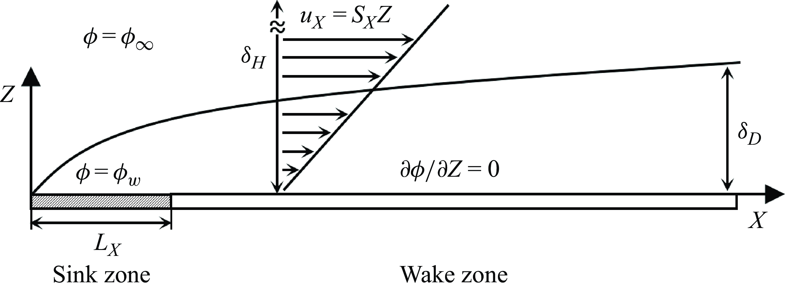


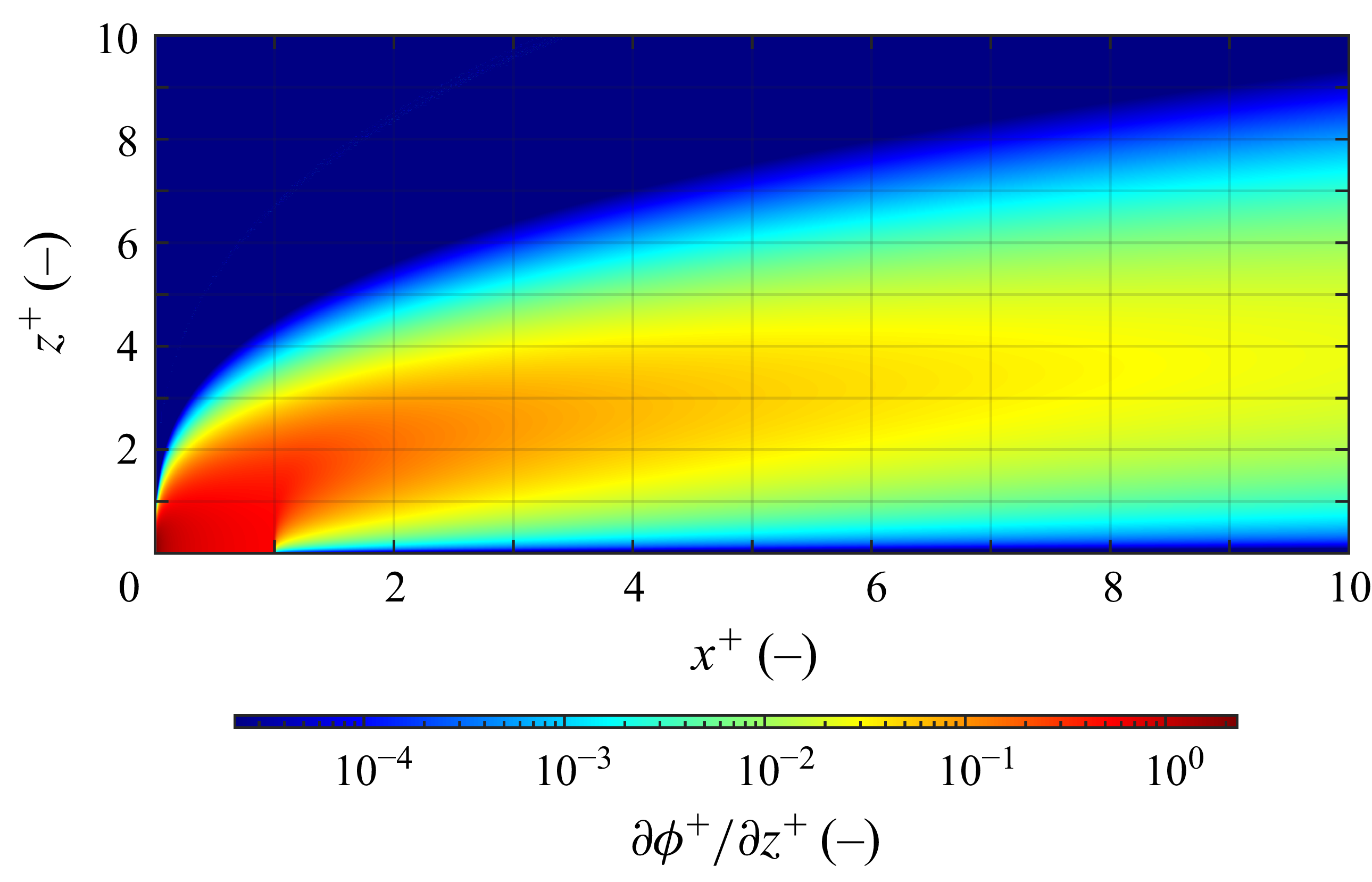

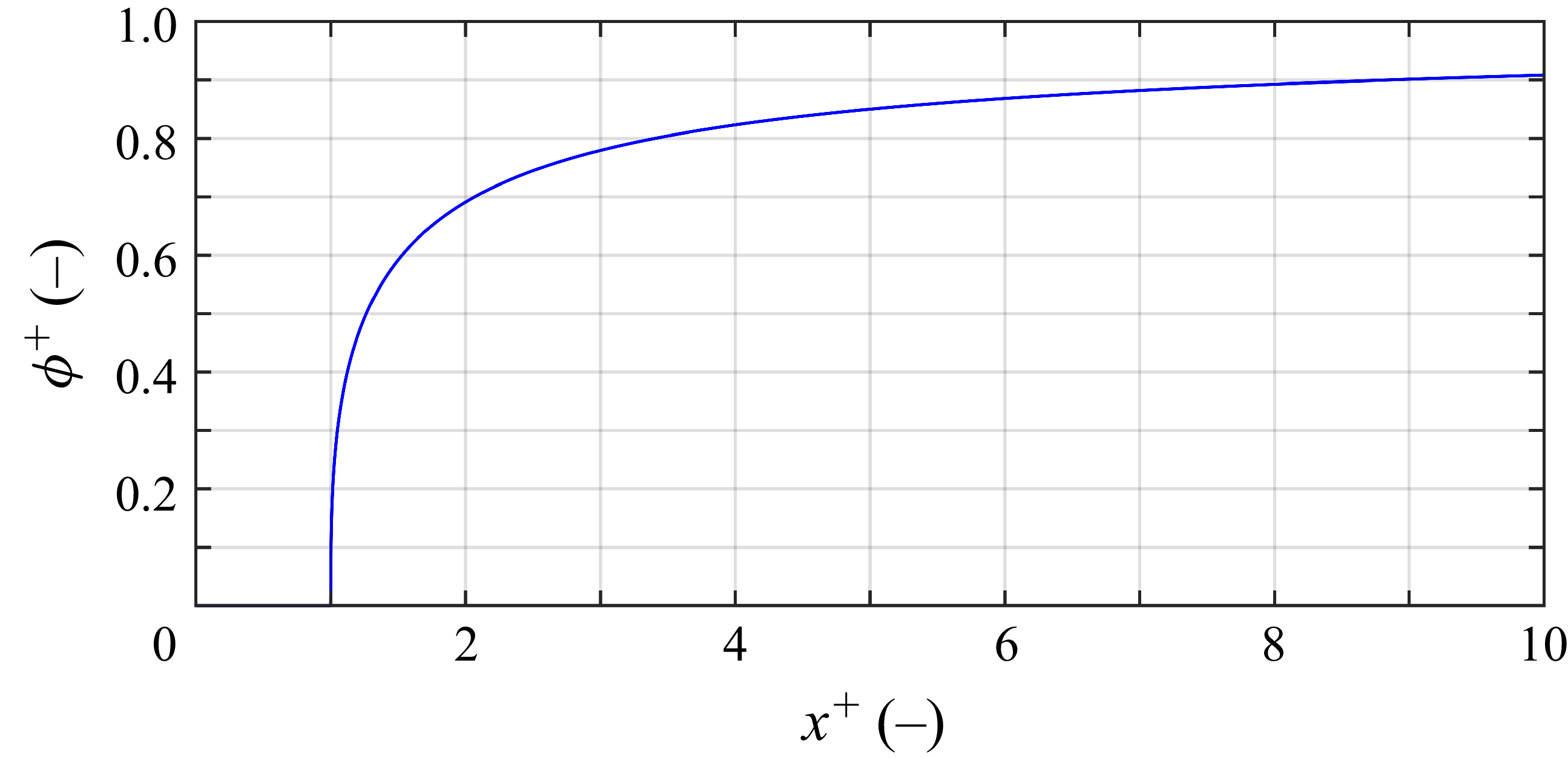


 Open access