


Introduction
As the performance requested to microwave devices develops to meet the demanding targets of the wireless industry, the need for fast and reliable design tools is ever increasing. In this framework, empirical High-Electron-Mobility Transistor (HEMT) modeling faces a number of challenges as Gallium Nitride (GaN) HEMT devices, which feature an unprecedented performance both in terms of power density as well as wideband operation [Reference Schuh, Sledzik, Reber, Widmer, Oppermann, Mußer, Seelmann-Eggebert and Kiefer1], are introduced at an industrial level [Reference Blanck, Thorpe, Behtash, Splettstößer, Brückner, Heckmann, Jung, Riepe, Bourgeois, Hosch, Köhn, Stieglauer, Floriot, Lambert, Favede, Ouarch and Camiade2]. Indeed, GaN devices show inherent low-frequency (LF) dispersive effects [Reference Santarelli, Cignani, Gibiino, Niessen, Traverso, Florian, Lanzieri, Nanni, Schreurs and Filicori3] that considerably impact their radio-frequency (RF) behavior in power amplifiers [Reference King and Brazil4] and RF switches [Reference Florian, Gibiino and Santarelli5] applications.
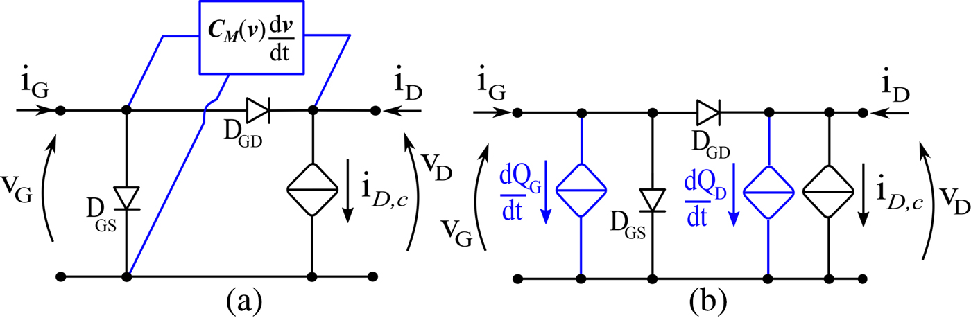
During the last years, modeling developments were mainly focused on the impact of LF dispersive phenomena on the conduction current [Reference King and Brazil4,Reference Avolio, Schreurs, Raffo, Crupi, Angelov, Vannini and Nauwelaers6–Reference Xu, Jones, Harris, Nielsen and Root11]. Lately, attention has been drawn to the influence that charge trapping may have on the displacement current modeling flow [Reference Wilson and King12], and the consequent impact on linearity performance prediction under modulated excitation, namely the prediction of intermodulation distortion (IMD) products. The description of the displacement current component involves choosing a suitable model representation, either in terms of nonlinear capacitances, as in Fig. 1(a), or by means of nonlinear charge functions, as in Fig. 1(b). Capacitive models, commonly implemented as equivalent-circuit models based on nonlinear capacitance lumped elements, are widespread for their immediate implementation and intuitive behavior. They can be described in a general way by considering a two-port capacitance matrix, whose elements can be directly extracted from small-signal measurements. Notably, implementing a model in terms of bivariate capacitances does not automatically guarantee terminal charge conservation, causing potential issues in circuit simulation [Reference Rudolph, Fager and Root13]. In time-domain circuit analysis, non-charge-conservative models may cause time-increasing integration errors in long transient simulations. In harmonic-balance (HB) simulation, a non-physical dc current is generated. Especially at the gate port, such a spurious dc component in the presence of the large impedance usually adopted in the gate bias network, might cause large spurious dc voltage errors that will, in turn, change the device operating point, affecting simulation accuracy. Therefore, despite not being a general requirement, terminal charge conservation is a highly desirable model feature. Given a general two-port capacitance matrix representation:
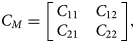 $${C_M} = \left[ {\matrix{{{C_{11}}} & {{C_{12}}}\cr {{C_{21}}} & {{C_{22}}}\cr } } \right],$$
where all elements depend on the controlling voltages v 1 and v 2, the two following additional constraints must be verified for terminal charge conservation [Reference Rudolph, Fager and Root13]:
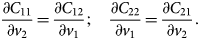 $${{\partial {C_{11}}} \over {\partial {v_2}}} = {{\partial {C_{12}}} \over {\partial {v_1}}};\quad {{\partial {C_{22}}} \over {\partial {v_1}}} = {{\partial {C_{21}}} \over {\partial {v_2}}}.$$
Conversely, a two-port charge model implementation involves identifying two charge functions. The displacement currents are obtained as time-derivatives of charge functions, so charge conservation is structural in this case.
(a) Intrinsic model based on the capacitance matrix. (b) Intrinsic model based on charge functions.
Either choosing a capacitive or a charge representation, a fundamental aspect concerns the empirical dataset for the identification. If such a dataset consists of small-signal S-parameters and the conditions in (2) are not verified, extracting a capacitive model will involve the aforementioned simulations issues, whereas the charge functions obtained by integration will not be unique, as they will depend on the voltage-domain integration path. In fact, since multi-bias small-signal S-parameters measurements are not isodynamic, the capacitance matrix does not satisfy the condition in (2) owing to the presence of dispersive phenomena [Reference Zucchelli, Santarelli, Raffo, Vannini and Filicori14]. On the other hand, also an extraction from large-signal (LS) excitation typically leads to a local model approximation, unless the excitation design follows specific constraints, as will be shown in the following. Thus, maximum care should be exercised when designing the identification experiments such that (i) the operating area is properly covered; (ii) the dataset is isodynamic, i.e., all empirical values used for model extraction belong to a specific and well-defined dynamic state. With respect to the latter, LF dispersion should be particularly taken care of.
This work, by extending the contribution in [Reference Gibiino, Santarelli and Filicori15], depicts a systematic procedure to obtain the most suitable charge-conservative GaN model that could be derived from non-isodynamic data. Such a method aims at providing fair performance prediction and the robust charge functions implementation for the many cases where special-purpose expensive setups capable to perform isodynamic experiments [Reference Niessen, Gibiino, Cignani, Santarelli, Schreurs and Filicori16,Reference Goncalves, Nunes, Cabral and Pedro17] are not available. The paper is organized as follows. The section “Large-signal identification for GaN” reviews the specific aspects related to GaN state dynamics and depicts an experiment for obtaining isodynamic datasets from steady-state LS measurements. In the section “Approximate modeling from non-isodynamic measurements”, the approach is exploited to extract approximate charge-conservative models, whose performance is evaluated in the section “Results and discussion”. Conclusions are drawn in the section “Conclusion”.
Large-signal identification for GaN
GaN HEMT state dynamics
GaN dispersive effects due to thermal and charge trapping phenomena involve complex electronic mechanisms within the device, showing (i) a combination of fast charge trapping mechanisms (some in the order of less than ns) and slow de-trapping transients (up to hundreds of ms); (ii) a nonlinear dependency of such dynamic behavior on the dynamically applied voltages, resulting in a composite nonlinear dynamic global response. This causes that, for example, when measuring a static current-voltage (IV) device characteristic, each bias point belongs to different thermal and charge trapping states. Therefore, classic multi-bias S-parameters cannot constitute an isodynamic dataset for charge functions extraction [Reference Zucchelli, Santarelli, Raffo, Vannini and Filicori14]. Although exploiting pulsed excitation for obtaining IV characteristics at fixed thermal state is straightforward, guaranteeing isodynamic conditions for GaN devices is less simple due to charge trapping [Reference Santarelli, Cignani, Niessen, Traverso and Filicori18]. To overcome the issue, different approaches can be followed.
The work in [Reference Santarelli, Cignani, Gibiino, Niessen, Traverso, Florian, Schreurs and Filicori19] exploits the peculiar trap dynamics to modify the pulsed excitations with a double-pulse pattern, where a pre-pulse is used to stabilize the regime to a pre-conditioned trapping state. Then, multi-bias double-pulsed S-parameters obtained with such a strategy can actually constitute an isodynamic dataset for charge and capacitance extraction [Reference Goncalves, Nunes, Cabral and Pedro20]. Alternatively, a direct way to guarantee the isodynamic property to the identification dataset consists in obtaining such a dataset from a unique LS steady-state regime [Reference Niessen, Gibiino, Cignani, Santarelli, Schreurs and Filicori16].
Optimal tone frequency selection
A number of published works has dealt with designing efficient LS excitation for capacitance or charge functions extraction [Reference Jansen, Schreurs, De Raedt, Nauwelaers and Van Rossum21–Reference Perez-Parras, Martin-Guerrero, Baños-Polglase and Camacho-Peñalosa25]. Exploiting the simultaneous excitation of the two ports of the device, they all aim at a dense and complete coverage of the operating v 1-v 2 voltage plane. In addition, multiple derivatives of the current with respect to the applied voltages should be sampled for each point of the v 1-v 2 voltage plane in order to identify the capacitance elements. These elements, along with the limitations of the measurement setup, help in drafting a list of desired features for the excitation. Let us consider a generic voltage-controlled N-port. Let  $f_1\ldots f_N$ be N independent tone frequencies, each of which is applied to the n-th port of the device. The generated IMD products will fall at the generic frequency $\sum\nolimits_{n=1}^{N} k_nf_n$, where 0 ≤ |k n| ≤ K n and $\sum\nolimits_{n=1}^{N} \vert k_n \vert\le K_{max}$, K n being the maximum harmonic order at the n-th port and K max the maximum mixing order. Thus, one should consider the following signal characteristics [Reference Niessen, Gibiino, Cignani, Santarelli, Schreurs and Filicori26]:
(i) All non-negligible (i.e., of lower mixing order, or equivalently, up to the maximum nonlinear order required) IMD products must be measurable.
(ii) Two (or more) IMD products should never fall on the same frequency bin. From a measurement perspective, they should not fall too close, so to minimize measurement inaccuracies.
(iii) The excitation should be applied in a frequency range where the displacement current component is non-negligible with respect to the conduction current.
(iv) Since the displacement current is obtained as a time-derivative of charge, $\min \{\sum\nolimits_{n=1}^{N} k_nf_n\}$ must be sufficiently high, in order to reduce current integration errors.
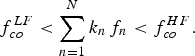
(v) The frequency response has to be frequency-confined between the upper cut-off of the LF dispersive phenomena
$f_{co}^{LF}$ and the lower cut-off of the high-frequency (HF) non-quasi-static effects $f_{co}^{HF}$:
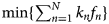


 $$f_{co}^{LF} < \sum\limits_{n = 1}^N {{k_n}} {\,f_n} < f_{co}^{HF}.$$
While (i) and (ii) concern the general feasibility of the measurement and (iv) relates to the extraction procedure, (v) can constitute a stringent condition for the specific case of GaN. From these specifications one realizes that, on one hand, it would be preferable to adopt a large frequency spacing between the tones, so that (ii) and (iv) would be easily satisfied. On the other hand, this is in contrast with (i) and (v) for which confining the spectral response is a must. By considering the case of a common-source transistor (N = 2), finding proper f 1 and f 2 will depend on a suitable value for K max which, in turn, depends on the nonlinearity involved. Nevertheless, it has been shown in [Reference Niessen, Gibiino, Cignani, Santarelli, Schreurs and Filicori26] that acceptable compromises can be found if using instrumentation with several-GHz-wide acquisition bandwidth (BW). In Fig. 2, we show the trace in the voltage plane and the drain current locus, as well as the excitation spectrum for the case of f 1 = 2 GHz, f 2 = 2.74 GHz, K 1,2 = 10, and K max = 20, determining a lower IMD at 220 MHz, well above the cut-off of the LF dispersive effects. Such an experiment can be performed by means of a Keysight PNA-X network analyzer, as shown in [Reference Niessen, Gibiino, Cignani, Santarelli, Schreurs and Filicori16].
Two-tone (one per port) excitation of a 0.25-μm GaN HEMT with f 1 = 2 GHz, f 2 = 2.74 GHz, K 1,2 = 10, and K max=20. (a) Voltage plane. (b) Drain current locus. (c) Excitation spectrum. (d) Zoom of (c) for frequencies up to 1 GHz.

An interesting aspect concerns the fact that such multiple sinusoidal excitations give origin to a complex trace in the voltage domain, also known as Lissajous curves.Footnote 1 In this way, the voltage domain can be widely covered, and each voltage region is passed through multiple times at different speeds, depending on the ratio between the applied frequencies. This, in turn, results in different time-derivatives of the output current, ultimately leading to charge functions identification. More in detail, the resulting regime is periodic with period  $T={1}/({GCD(f_{1},\ldots ,f_{N})}$, where GCD( · ) calculates the greatest common divisor among the applied frequencies. Therefore, T is a time interval in which the traced path will return to the initial point, and it is also the minimum acquisition time for the measurement. If no greatest common divisor can be calculated, then the signal is an almost periodic multi-tone, and it will produce a trajectory that never repeats itself.
Frequency-domain integration
The experiment depicted in the previous section results in L ≤ N current waveforms (L being the number of considered output ports), each of which can be depicted by an N-dimensional Fourier series:
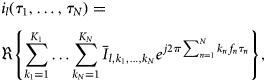 $$\eqalign{ & {i_l}({\tau _1}, \ldots ,{\tau _N}) = \cr & \Re \left\{ \sum\limits_{{k_1} = 1}^{{K_1}} \ldots \sum\limits_{{k_N} = 1}^{{K_N}} {{{\bar{I}}_{l,{k_1}, \ldots ,{k_N}}}} {e^{\,j2\pi \sum\nolimits_{n = 1}^N {{k_n}} {\,f_n}{\tau _n}}}\right \} , \cr} $$
where  $l=1\ldots\; L$, and $\bar {I}_{l,k_1,\ldots ,k_N}$ are the Fourier coefficients relative to the current at the l-port. Given that current is the time-derivative of the charge, charge values must be obtained by integration of the displacement current, whereas the global current response in (4), in general, contains both conductive and displacement current components. This is indeed the case for the drain port of the transistor, whereas the gate port typically contains only a displacement part if the gate diodes are not turned on. The displacement current can be separated from the conduction current at the drain port by following different strategies, e.g., the one in [Reference Niessen, Gibiino, Cignani, Santarelli, Schreurs and Filicori16].
Once any conductive part has been removed, the pure displacement currents can be integrated in the frequency domain, directly obtaining the spectral components of the charges:
 $${\bar{Q}_{l,{k_1}, \ldots ,{k_K}}} = {{{{\bar{I}}_{l,{k_1}, \ldots ,{k_N}}}} \over {\,j2\pi \sum\limits_{n = 1}^N {{k_n}} {\,f_n}}},$$
which can be transformed to time domain by means of the N-dimensional Fourier Series:
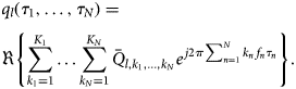 $$\eqalign{& {q_l}({\tau _1}, \ldots ,{\tau _N}) = \cr & \Re \left \{ \sum\limits_{{k_1} = 1}^{{K_1}} \ldots \sum\limits_{{k_N} = 1}^{{K_N}} {{{\bar{Q}}_{l,{k_1}, \ldots ,{k_N}}}} {e^{\,j2\pi \sum_{n = 1}^N {{k_n}} {\,f_n}{\tau _n}}}\right \} . \cr} $$
Obtaining the charge functions
Each of the time-domain charge loci in (6) depends on the time-domain voltage loci at all ports:
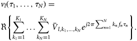 $$\eqalign{& {v_l}({\tau _1}, \ldots ,{\tau _N}) = \cr & \Re \left \{ \sum\limits_{{k_1} = 1}^{{K_1}} \ldots \sum\limits_{{k_N} = 1}^{{K_N}} {{{\bar{V}}_{l,{k_1}, \ldots ,{k_N}}}} {e^{\,j2\pi \sum\nolimits_{n = 1}^N {{k_n}} {\,f_n}{\tau _n}}}\right \} . \cr} $$
If the charges constitute an exact differential in the voltage domain, the  $q_l(\tau _1,\ldots ,\tau _N)$ must give origin to N quasi-static functions of the $v_1,\ldots ,v_n$ controlling voltages, i.e., the charge functions. Such functions, indicated with $Q_l[v_1,\ldots ,v_n]$, are therefore defined by establishing an explicit correspondence between each point in the voltage domain and the respective value of waveforms q l. If the excitation frequencies are properly defined, a sufficiently dense distribution of the traced paths in the voltage domain is obtained. In addition, the Fourier series expressions in (6) and (7) allow for any arbitrarily dense discretization of such time-domain paths. This discretization corresponds by all means to an interpolation, as the time domain signals are completely known from their frequency-domain components. In this sense, it is worth bearing in mind that the choice for the maximum harmonic order for each output (K n) and the maximum IM order (K max) sets a limit to the nonlinearity order of the identified charge functions. In practice, the data points of q l and v l obtained from the discretization of (6) and (7), respectively, can be used in conjunction with suitable functions approximator algorithms, e.g., [Reference D'Errico27], to fully characterize the $Q_l[v_1,\ldots ,v_n]$ functions.Let us now consider the case of a transistor in common-source configuration, which is represented as a two-port (N = L = 2). Figure 3 shows q 1 and q 2 loci for the gate and the drain ports, along with the identified 2-dimensional charge functions (renamed Q G for the gate port and Q D for the drain port). Whereas the described identification technique has been applied in [Reference Niessen, Gibiino, Cignani, Santarelli, Schreurs and Filicori16] from LS measurements, the next section deals with the use of the same model extraction principles in conjunction with experimental datasets acquired in small-signal regime.
Time-domain locus of the charges and relative charge functions obtained from the excitation in Fig. 2. (a) Gate charge. (b) Drain charge.

Approximate modeling from non-isodynamic measurements
Description of the approach
As already mentioned in the Introduction, different integration paths applied to capacitances identified from non-isodynamic measurements will generally lead to different charge functions, whereas a unique charge function per port must be implemented. On the other hand, non-isodynamic datasets such as multi-bias S-parameters contain a great amount of information on the dynamics involved, as the IMD prediction of models based on capacitance matrix shows [Reference Santarelli, Niessen, Cignani, Gibiino, Traverso, Florian, Schreurs and Filicori7]. Therefore, it is worth investigating the extraction of such valuable information to obtain optimal charge functions from a suboptimal dataset, maintaining the prediction capabilities. In this sense, selecting the most appropriate integration path becomes a critical step.
The strategy proposed in this work consists in exciting, by simulation, a non-charge-conservative transistor model obtained from a non-isodynamic dataset in a suitable way. This allows to condition the extraction to be coherent with respect to the intended application, employing all the principles described in the section “Large-signal identification for GaN” for limiting the BW of the excitation to the range where displacement currents give the most important contribution. Finally, this also indirectly sets a suitable integration path that efficiently sweeps the operating area within the experimental dataset. The proposed procedure consists of the following steps:
(i) Perform conventional multi-bias S-parameter measurements on a dense grid of bias voltages and over a suitable frequency range where displacement currents arise. These measurements require exciting only a small-signal regime and they are normally obtained by means of a Vector Network Analyzer (VNA), typically present in any microwave laboratory.
(ii) De-embed parasitics [Reference Dambrine, Cappy, Heliodore and Playez28], extract the capacitance matrix of the model in Fig. 1(a) from the Y-parameters, and implement the network in the schematic circuit of an HB simulator. The capacitive matrix can be simply implemented by means of a Look-Up Table (LUT), as in [Reference Santarelli, Niessen, Cignani, Gibiino, Traverso, Florian, Schreurs and Filicori7]. The conduction current can be extracted in an independent way. In this work, we have used the conduction current model in [Reference Gibiino, Santarelli and Filicori29], while the thermal model consists of a thermal resistance (
$R_\theta \simeq 13^{\circ }{\rm C/W}$) obtained with the method in [Reference Florian, Santarelli, Cignani and Filicori30].(iii) Setup an HB simulation of the implemented circuit to perform a two-tone simulation experiment (Fig. 4), where the excitation frequencies should be selected by following the indications of the section “Optimal tone frequency selection”. This simulation provides, as an output, wideband spectra of the voltages and currents at the device ports, which can be transformed in time domain to evaluate the actual paths traced on the device characteristics. It should be noted that, despite such a non-charge-conservative model will generate a non-physical dc component of the current, this component is automatically discarded in the analysis.
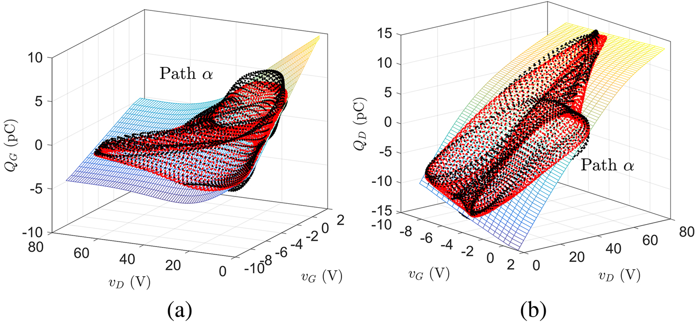
(iv) Extract the charge functions by means of the procedure in the section “Obtaining the charge functions”. Since the extraction relies, in general, on non-isodynamic data, the time-domain charge loci may not represent a sampling of a quasi-static function of the voltages, showing hysteresis. Moreover, spurious memory effects may arise due to the restricted BW deriving from the practically-limited mixing order. In this sense, a function approximator [Reference D'Errico27] that best fits the available data is necessary. In Fig. 5, the differences are shown between the actual loci of the charges (black) and the points on the approximated surface (red) for the case of a simulation experiment (excitations as from Fig. 2).

Harmonic-balance simulation setup (Keysight ADS) for the implementation of the two-tone experiment.

Charge function fitting from the time domain charge locus (black) traced by path α. In red, the projection of the locus on the actual approximated charge surface. (a) Gate charge. (b) Drain charge.
Description of the simulation experiments
To test the approach, various simulation experiments have been configured. By selecting different excitations at the two ports, different shapes and temporization of the paths traced in the controlling voltage domain are synthesized, so that different probings of the device response can be evaluated. Given that the capacitance-based model obtained from S-parameters measurements is not charge conservative, such different excitations lead, in general, to the identification of different charge functions. Therefore, these tests allow to quantify such differences and estimate how much this suboptimal extraction dataset will affect the accuracy of the model.
As a preliminary step, the S-parameters of a 8× 125, 0.25-μm GaN-on-SiC HEMT were measured from 100 MHz up to 30 GHz by means of an 8510 Keysight VNA. A standard RLC π-network of extrinsic parasitic elements was extracted by means of the method in [Reference Dambrine, Cappy, Heliodore and Playez28] (R G = 0.9 Ω, R D = 1.6 Ω, R S = 0 Ω; L G = 140 pH, L D = 104 pH, L S = 8 pH, C GS = 28 fF, C DS = 65 fF, C GD = 0 fF). The capacitance elements extracted from the de-embedded measurements have been implemented in the auxiliary capacitive model of Fig. 1(a) and the schematic of Fig. 4. Then, different sinusoidal excitationsFootnote 2 were applied in the simulations for obtaining:
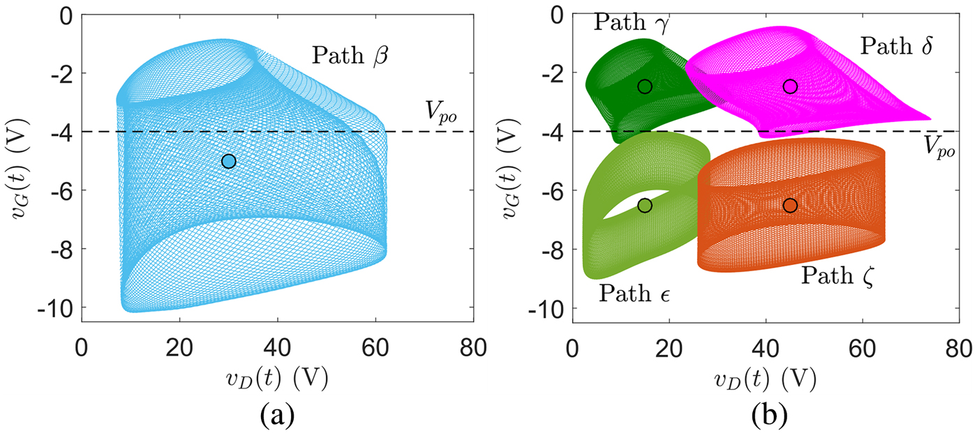
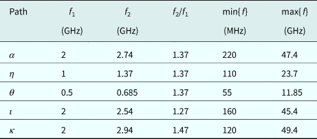
(i) Different operating areas. These can be configured by selecting different bias points and different amplitudes for the excitations signals. In this work, we have configured six different excitations α to ζ, whose parameters are reported in Table 1. While the shape of the α path was already provided in Fig. 2, the others are reported in Fig. 6, showing the different coverages of voltage domain, both above and below the pinch-off voltage V po of the device.
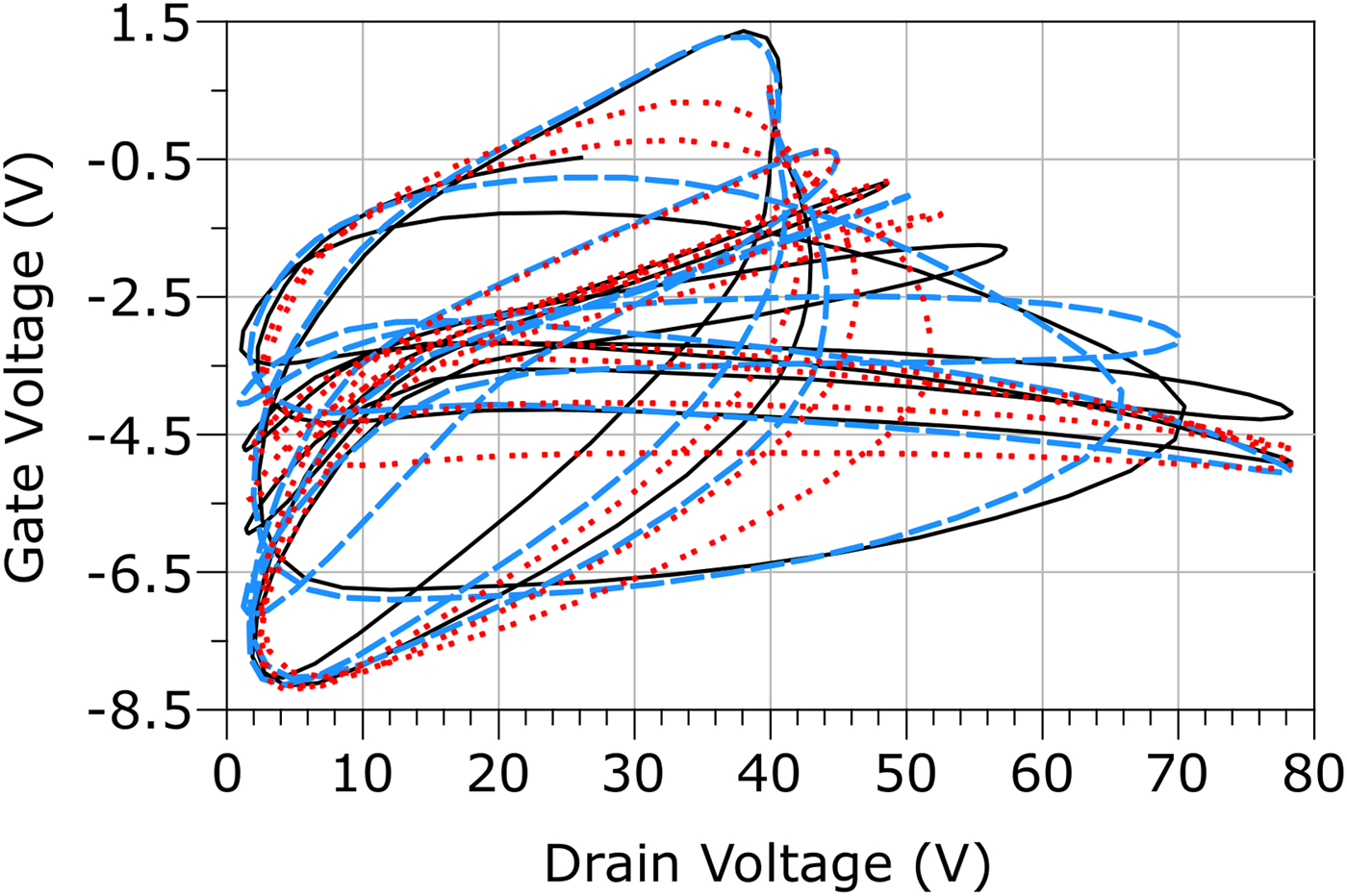
(ii) Different excitation frequencies. These can influence both the shape of the synthesized path, as well as the speed rate at which the path is passed through. In particular, the shape of the path depends on the ratio between the two excitation frequencies. The applied excitations and the resulting paths (η to κ) are reported in Table 2, while the amplitude levels of the excitations are kept the same as the ones for α. The paths η and θ maintain the same frequency ratio as α, so the shape of the path remains the same, while the speed at which this is passed through is 2 × slower for η (T = 100 ns) and 4 × slower for θ (T = 200 ns). Such temporization differences can be clearly seen in the frequency domain, as shown in Figs 7(a) and 7(b). For ι and κ, the frequency ratio is changed, so that the traced paths change, as shown in Fig. 8.
Paths generated in the voltage plane. (a) Excitation β. (b) Excitations γ, δ, ε, and ζ.
Spectrum response for the paths η, θ, ι, and κ.

Paths α (black solid line), ι ( blue long dash), and κ (red dot) in the voltage plane for an observation time of 2.5 ns.
Integration paths for different excitation amplitudes

Integration paths for different frequencies
Results and discussion
Charge functions approximation
After the dynamic voltage and currents are saved for the α to κ configurations depicted in the previous section, two time-domain charge waveforms q G and q D (for gate and drain) are extracted for each case by integrating the displacement currents in frequency domain. Then, these are fitted to two 2-dimensional surfaces in the v G-v D variables. Given that some of the synthesized loci do not cover the full operating area in the voltage plane, the resulting charge functions will only be evaluated within the respective limited domain. An interesting metric to consider is the fitting relative error to the surface E F:
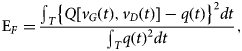 $${{\rm{E}}_F} = {{{\int _T}{{\left\{ {Q[{v_G}(t),{v_D}(t)] - q(t)} \right\}}^2}dt} \over {{\int _T}q{{(t)}^2}dt}},$$
where Q[v G(t), v D(t)] is the approximated charge surface, q(t) is the time-domain charge locus, and T is the period of the excitation. If all the values of q G(t) and q D(t) were perfectly laying on a surface, such fitting error would be zero. Conversely, the presence of a fitting error means that the sampled charge data points do not perfectly belong to a quasi-static function of the applied voltages. Therefore, this indicates that such sampled charges depend on the traced path, due to the different dynamic states at which the S-parameter dataset was acquired.
The fitting error for the different excitations used in this work is shown in Fig. 9. It can be seen that, for all paths, a certain fitting relative error up to 12% is present, and that such an error is generally larger for Q G with respect to Q D. Notably, the error is lower for the β, γ, ε, and ζ paths, which are obtained either by biasing the device below pinch-off, or at relatively low drain voltage for γ (i.e., in zero or low-power dissipation conditions). This aspect seems in agreement with the general principle for which operating temperature and trap state differences, particularly evident for high quiescent voltages and currents, will change the state of the device, thus making the multi-bias S-parameters non-isodynamic.
(a) Gate charge surface fitting error (%). (b) Drain charge surface fitting error (%).

It is worth noting that a small surface fitting error does not directly mean that a unique charge function has been obtained from different excitation conditions. In fact, the different paths could generate charge signals laying on different surfaces. To clarify this aspect, the following relative error between the approximated charges has been calculated:
 $${{\rm{E}}_Q} = {{\int {\int _{{D_v}}}{{\left\{ {Q[{v_G},{v_D}] - \hat{Q}[{v_G},{v_D}]} \right\}}^2}d{v_G}d{v_D}} \over {\int {\int _{{D_v}}}\hat{Q}{{[{v_G},{v_D}]}^2}d{v_G}d{v_D}}},{\rm{ }}$$
where  $\hat {Q}[v_G,v_D]$ is a reference charge function and D v is the voltage domain corresponding to each path. The resulting values of EQ are shown in Fig. 10. For the charge functions obtained by biasing the HEMT in the ON-state, i.e., γ, δ, η, θ, ι, and κ, the chosen reference charge functions are the ones extracted by the configuration α. For the charge functions obtained by biasing below pinch-off, i.e., ε and ζ, the reference charge functions are the ones obtained with the configuration β.
(a) Relative errors of the charge functions obtained for paths γ, δ (referred to the ones obtained from path α), ε, ζ (referred to the ones obtained from path β). (b) Relative errors of the charge functions obtained for paths η, θ, ι, κ (referred to the ones obtained from path α).
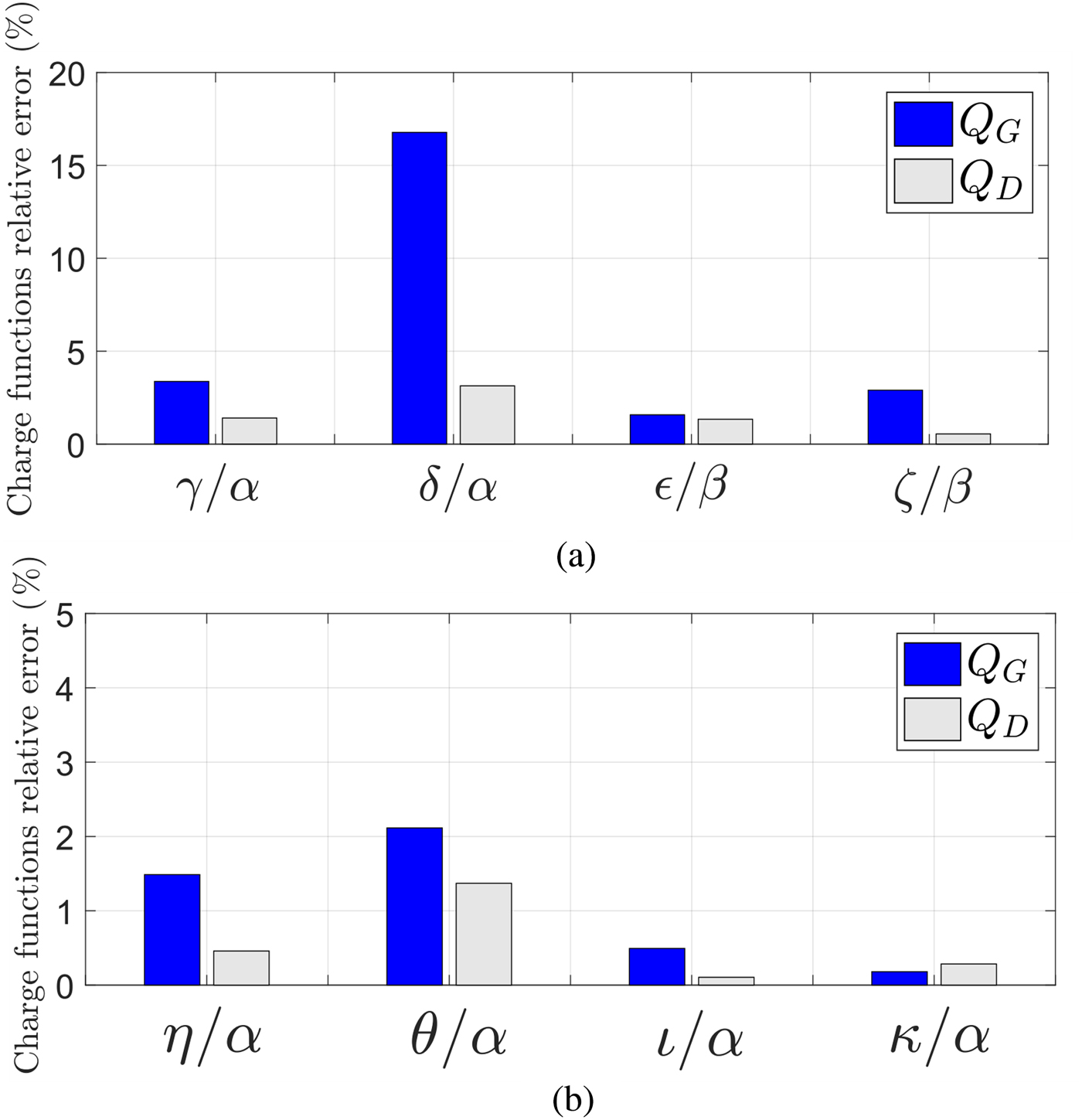
It can be noted that the gate charge function obtained from δ reports more than 15% in relative error with respect to α. This means that the fitting error shown in Fig. 9 has caused the synthesis of two different charge models. On the other hand, despite the gate charges from paths η to κ (as well as α) were showing substantial fitting error, the approximated charge models they provide are quite similar to each other, originating only up to ~ 2% of relative error. Apart from the gate charge from δ, the different charge models only show a few percent of relative error. This means that, despite having been obtained from different excitations of a non-isodynamic dataset, they are relatively similar to each other.
Small-signal behavior
In order to evaluate their prediction capabilities, the charge functions have been implemented in CAD (Keysight ADS), giving origin to ten different charge models. Such implementations take advantage of the Symbolically-Defined Device (SDD) component, which allows to calculate the derivatives of the quantities applied to its terminals. Considering HB simulations, this corresponds to a multiplication by frequency at each frequency. Then, once the derivatives are obtained in the frequency domain, they can be transformed to time domain. In the specific case, the charge functions covering a suitable operating area are read from LUTs. Then, the output of the LUTs is directly applied to the SDD for obtaining the corresponding displacement currents. Alternatively, it would be possible to synthesize conventional equivalent-circuit model topologies from the same identified charge functions.
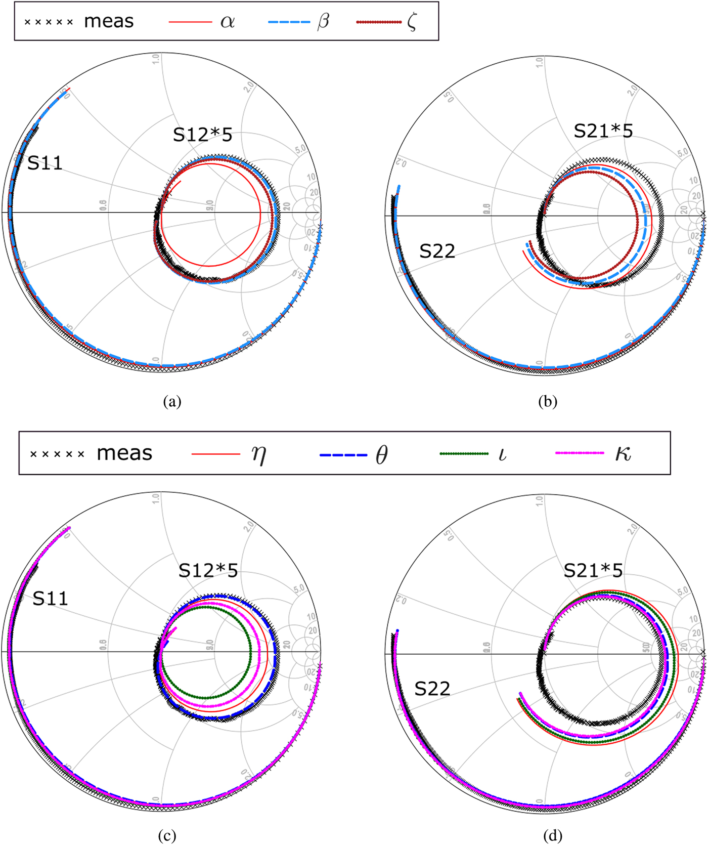
As a first test, such newly obtained models have been simulated to extract the S-parameters at different bias points. These simulations, performed in the [0.1,30] GHz range, have been compared to the actual S-parameters measurements, and are shown in Figs. 11–13. In particular, three bias points have been considered: (V GQ, V DQ) = (− 3, 15) V (Fig. 11), (V GQ, V DQ) = (− 3, 30) V (Fig. 12), both in the ON-state, and (V GQ, V DQ) = (− 6, 30) V (Fig. 13) in pinch-off. Despite the relative differences between the charge functions obtained, the S-parameters predicted by the models are fairly similar to the measurements. In particular, it can be noted that the S 11 is well predicted in all conditions. In the ON-state conditions, the S 21 is fairly aligned for the V DQ = 15 V, whereas it shows larger errors for V DQ = 30 V. In fact, despite the model extraction derives from the very same S-parameter measurements, and although charge should not be affected by LF dispersion [Reference Niessen, Gibiino, Cignani, Santarelli, Schreurs and Filicori16], it should be noted that the model identification is based on the LS evaluation of the measured non-isodynamic dataset, introducing spurious deviations. Therefore, as it was already mentioned concerning the fitting error of the δ gate charge, the prediction errors are likely to be larger in those areas where LF dispersion particularly manifests itself, i.e., at higher drain voltages. Thus, the most pronounced differences can be seen at V DQ = 30 V for S 22, being S 22 the most susceptible parameter with respect to thermal and trapping effects. Conversely, all the S-parameters are adequately reproduced when biasing in pinch-off, despite some minor disagreements in S 12 and S 21 among the various models.
Comparison between simulated and measured S-parameters at ON-state bias point V GQ = −3 V, V DQ = 15 V for f = [0.1 30] GHz. (a)–(b) S-parameters obtained with models derived from paths α, β, γ. (c)–(d) S-parameters obtained with models derived from paths η, θ, ι, κ.

Comparison between simulated and measured S-parameters at ON-state bias point V GQ = −3 V, V DQ = 30 V for f = [0.1, 30] GHz. (a)–(b) S-parameters obtained with models derived from paths α, β, δ. (c)–(d) S-parameters obtained with models derived from paths η, θ, ι, κ.

Comparison between simulated and measured S-parameters at OFF-state bias point V GQ = −6 V, V DQ = 30 V for f = [0.1, 30] GHz. (a)–(b) S-parameters obtained with models derived from paths α, β, ζ. (c)–(d) S-parameters obtained with models derived from paths η, θ, ι, κ.
Large-signal behavior
Figure 14 shows the prediction of the dc current by the capacitance-based model in comparison with the charge-based model (obtained from path α) for a continuous wave (CW) excitation at 5.5 GHz. It can be seen that the newly implemented charge-based model do not produce any non-physical dc current, whereas the capacitance model is likely to suffer from the simulation issues discussed in the Introduction.
Comparison between the α charge-based (charge-conservative) and the capacitance-based (non-charge-conservative) dc current model response (diodes bypassed) for a single-tone excitation at 5.5 GHz up to 4-dB gain compression, with (V GQ, V DQ) = (− 3.4, 30) V, corresponding to I DQ ≃ 60 mA. (a) Gate current. (b) Displacement part of the drain current.

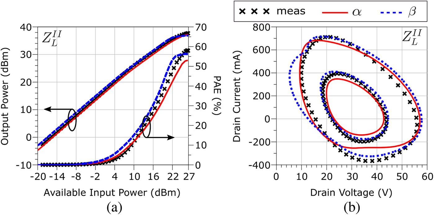
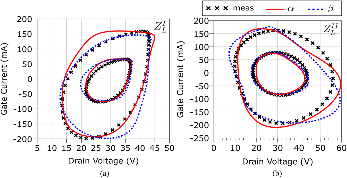
Two loading conditions are considered for the LS validation:  $Z_{L}^{I}\simeq $ 50 Ω, with harmonics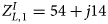 $Z_{L,1}^{I}=54+j14$, $Z_{L,2}^{I}=53+j19$,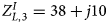 $Z_{L,3}^{I}=38+j10$, and $Z_{L}^{II}$ (maximum RF output power), with harmonics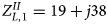 $Z_{L,1}^{II}=19+j38$,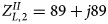 $Z_{L,2}^{II}=89+j89$,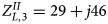 $Z_{L,3}^{II}=29+j46$. Figures 15–17 show the α and β model performance in the presence of an RF CW excitation at 5.5 GHz. For all tests, the chosen quiescent point is (V GQ, V DQ) = ( − 3.4, 30) V, corresponding to I DQ ≃ 60 mA. The obtained results confirm good prediction capabilities for both loads, in terms of RF output power, power-added efficiency (PAE), as well as for the IV waveforms. The CW performance for the models extracted from $\eta ,\theta ,\iota $ and κ (not shown) is basically the same as for the α model.
(a) Prediction of RF output power and power-added efficiency (PAE) for the models extracted from the α and β paths in the presence of an RF CW at 5.5 GHz and load  $Z_{L}^{I}\simeq $ 50 Ω (harmonics: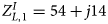 $Z_{L,1}^{I}=54+j14$,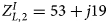 $Z_{L,2}^{I}=53+j19$, $Z_{L,3}^{I}=38+j10$). (b) Loadline prediction for two RF input levels: 16 and 24 dBm.

(a) Prediction of RF output power and power-added efficiency (PAE) for the models extracted from the α and β paths in the presence of an RF CW at 5.5 GHz and load  $Z_{L}^{II}$ for maximum output power (harmonics: $Z_{L,1}^{II}=19+j38$,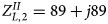 $Z_{L,2}^{II}=89+j89$, $Z_{L,3}^{II}=29+j46$). (b) Loadline prediction for two RF input levels: 16 and 24 dBm.
Gate current prediction for the α and β models in the presence of a CW excitation at 5.5 GHz and RF input levels 16 and 24 dBm. (a)  $Z_{L}^{I}\simeq 50\,\Omega $. (b) $Z_{L}^{II}$ for maximum RF output power.
As a last test, the charge-based models have been excited by a standard two-tone excitation (both applied at the same port) in order to characterize the in-band 3rd order IMD products (IM3) for the  $Z_{L}^{II}$ load. As can be seen from Fig. 18, all results provide reasonable predictions, despite some slight variations among the different model implementations.
Prediction of the third-order intermodulation distortion products by using the different charge functions models (Δf = 20 MHz around 5.5 GHz.) with  $Z_{L}^{II}$ load for maximum RF output power. (a) Prediction with models from paths α and β. (b) Predictions with models from paths η, θ, ι, and κ.

Conclusion
In this work, we have described a method to obtain a GaN HEMT charge-conservative model from classic S-parameters measurements, thus avoiding the use of custom setups for isodynamic acquisitions. The proposed procedure involves simulating an auxiliary capacitive model with suitable two-tone excitations, resulting in a charge functions formulation that is charge-conservative by definition. Such obtained model could then be possibly mapped into equivalent-circuit topologies that still maintain terminal charge conservation. The small- and large-signal validations show that, despite some differences in the performance with respect to measurements, the obtained models provide good prediction consistency and a robust CAD implementation.
Author ORCIDs
Gian Piero Gibiino, 0000-0002-1261-9527.
 Gian Piero Gibiino received the dual Ph.D. degree from the University of Bologna, Bologna, Italy, and KU Leuven, Leuven, Belgium, in 2016. Since 2012, he has been with the Department of Electrical, Electronic, and Information Engineering “Guglielmo Marconi” (DEI), University of Bologna, where he is currently a Post-Doctoral Research Fellow. In 2016, he was a Visiting Researcher with Keysight Technologies, Aalborg, Denmark. His current research interests include the characterization and empirical modeling of microwave devices and systems, microwave measurements, and RF instrumentation.
 Alberto Santarelli received the Laurea degree (cum laude) in electronic engineering in 1991 and the Ph.D. in Electronics and Computer Science from the University of Bologna, Italy in 1996. He was a Research Assistant from 1996 to 2001 with the Research Centre for Computer Science and Communication Systems of the Italian National Research Council (IEIIT-CNR) in Bologna. In 2001, he joined the Department of Electrical, Electronic and Information Engineering “Guglielmo Marconi” (DEI), University of Bologna, where he is currently an Associate Professor. During his academic career he has been a Lecturer of Applied Electronics, High-frequency Electronics and Power Electronics. His main research interests are related to the nonlinear characterization and modeling of electron devices and to the nonlinear microwave circuit design.
 Fabio Filicori received the M.S. degree in electronic engineering from the University of Bologna, Bologna, Italy, in 1974. In the same year he joined the Department of Electronics, Computer Science and Systems, University of Bologna, initially as Research Assistant, and then as an Associate Professor. In 1990 he became Full Professor with the University of Perugia, Perugia, Italy. In 1991 he joined the University of Ferrara, Ferrara, Italy. In 1993, he joined again the University of Bologna. He has been a member of the Space Technology Committee of the Italian Space Agency and responsible for several research projects for the Italian National Research Council. He was TPC chair of the EuMIC conference in 2009. During his academic career, he has held courses on CAD, electron devices and circuits, and power electronics. His main research activities are in the areas of CAD techniques for nonlinear microwave circuits, electron device nonlinear modeling, sampling digital instrumentation and power electronics. After retiring in 2016, he is still involved in teaching and research activities at the University of Bologna as an adjunct professor.



