





1. Introduction
At the interface of a moving fluid and a solid surface, there exists a thin region referred to as a boundary layer. For high flow speeds, the boundary layer may become turbulent and becomes responsible for imparting fluctuating pressures on the solid surface beneath it. Quantifying the statistical nature of these pressure fluctuations is of great importance for the design, modelling, and understanding of how large structures and vehicles interact with fluid flow. There are two primary ways to describe the statistical nature of the pressure fluctuations in a boundary layer: (i) the single-point wall-pressure spectrum and (ii) the wall-pressure wavenumber–frequency spectrum. The single-point pressure spectrum gives a measure of the power of the pressure fluctuations across a range of frequencies. However, this does not provide any information about spatial scales, which are relevant for practical flows. For this reason, the wavenumber–frequency spectrum is a more useful tool for understanding the pressure fluctuations in a turbulent boundary layer. The wavenumber–frequency spectrum can be subdivided into four primary regions: (i) the convective region, wherein for a given frequency, the wavenumber is approximately equal to the convective wavenumber, $k_{c} = 2\pi f/U_{c}$
; (ii) the acoustic region, resulting from sound waves and pressure fluctuations whose trace speed is supersonic; (iii) the sub-convective region, which exists between the convective region and the acoustic cone; and (iv) the super-convective regime between the convective line and the abscissa, which is where the wavenumber is larger than the convective wavenumber,
$k_{c} = 2\pi f/U_{c}$
; (ii) the acoustic region, resulting from sound waves and pressure fluctuations whose trace speed is supersonic; (iii) the sub-convective region, which exists between the convective region and the acoustic cone; and (iv) the super-convective regime between the convective line and the abscissa, which is where the wavenumber is larger than the convective wavenumber, $k_{c}$
. The streamwise wavenumber–frequency spectrum of a smooth-wall boundary layer, as measured by Damani et al. (Reference Damani, Butt, Totten, Devenport and Lowe2025a
), is given in figure 1(b). The black dashed line represents the large-scale convective line (
$k_{c}$
. The streamwise wavenumber–frequency spectrum of a smooth-wall boundary layer, as measured by Damani et al. (Reference Damani, Butt, Totten, Devenport and Lowe2025a
), is given in figure 1(b). The black dashed line represents the large-scale convective line ( $k_{c} = 2\pi f/U_{c}$
,
$k_{c} = 2\pi f/U_{c}$
, $\omega _{c} = k_{1}U_{c}$
), the black dotted line represents the true convective line and the red dashed line represents the sound line (
$\omega _{c} = k_{1}U_{c}$
), the black dotted line represents the true convective line and the red dashed line represents the sound line ( $k_{a} = 2\pi f /c_{0}$
). The sub-convective region is the region between these acoustic and convective lines. It has been shown that sub-convective pressure fluctuations couple most strongly with the fundamental structural modes of many vehicles of interest, such as large-scale aircraft and marine vehicles (Chang, Piomelli & Blake Reference Chang, Piomelli and Blake1999; Lauchie & Park Reference Lauchie and Park2000). This coupling induces vibrations in the structure beneath the boundary layer, which leads to cabin noise and far-field sound radiation.
$k_{a} = 2\pi f /c_{0}$
). The sub-convective region is the region between these acoustic and convective lines. It has been shown that sub-convective pressure fluctuations couple most strongly with the fundamental structural modes of many vehicles of interest, such as large-scale aircraft and marine vehicles (Chang, Piomelli & Blake Reference Chang, Piomelli and Blake1999; Lauchie & Park Reference Lauchie and Park2000). This coupling induces vibrations in the structure beneath the boundary layer, which leads to cabin noise and far-field sound radiation.
(a) Magnitude of the cross-spectral density of wall-pressure fluctuations and (b) streamwise wavenumber–frequency spectrum of wall-pressure fluctuations measured in a smooth-wall boundary layer (adapted from Damani et al. Reference Damani, Butt, Totten, Devenport and Lowe2025a ).

Models of both the pointwise spectrum and the wavenumber–frequency spectrum have attempted to quantify these pressure fluctuations; however, there have continued to be significant discrepancies between these models and measured data (Graham Reference Graham1997; Blake Reference Blake2017). These discrepancies are particularly apparent for sub-convective pressure fluctuations, which drive the need for low uncertainty measurements targeted at this regime. Additionally, in real-world flows, roughness is ubiquitous due to many different effects such as icing, surface debris and corrosion. This surface roughness impacts the boundary layer by increasing the frictional resistance experienced near the wall, in turn increasing the boundary layer thickness, reducing the convection speed and increasing the amount of noise generated by the boundary layer pressure fluctuations. Measurements of the single-point wall-pressure spectrum in rough-wall turbulent boundary layers have been completed in the past; however, there continues to be disagreement about how to most accurately model this phenomenon (Blake Reference Blake2017; Catlett et al. Reference Catlett, Bryan, Chang, Hemingway and Anderson2021; Fritsch et al. Reference Fritsch, Vishwanathan, Roy, Todd Lowe and Devenport2023). Furthermore, experimental data pertaining to the continuous streamwise wavenumber–frequency spectrum have never been collected for rough-wall boundary layers, with only some measurements for specific wavenumber–frequency combinations available (Farabee & Geib Reference Farabee and Geib1991). For these reasons, new measurements of the continuous streamwise wavenumber–frequency spectrum are required to build robust models for the prediction of pressure fluctuations in rough-wall turbulent boundary layers.
Measurements of the wall-pressure spectrum in rough-wall turbulent boundary layers are difficult due to the presence of the roughness, especially when the goal is to measure sub-convective pressures whose amplitude is many orders of magnitude lower than the dominant convective pressure fluctuations. Single-point measurements can be achieved with relative ease through the use of surface-mounted microphones. However, Joseph (Reference Joseph2017) has shown that the single-point spectrum measured at the top of the roughness varies drastically from a measurement made flush with the underlying surface, so this must be considered. Two-point measurements become significantly more challenging in the presence of roughness because sensor spacing is dictated by the specific roughness configuration of the surface. For smooth walls, there have been many attempts to measure the wavenumber–frequency spectrum with various methods; however, many of these methods are not feasible in the presence of roughness. One approach is to use a linear array of pressure transducers, such as those used by Maidanik & Jorgensen (Reference Maidanik and Jorgensen1967). However, this cannot be easily replicated for rough-wall flows because sensor spacing will be impacted by roughness too greatly, thus leading to poor resolution in the wavenumber domain, or producing data only at specific wavenumber–frequency pairs. Farabee & Geib (Reference Farabee and Geib1991) used this technique for rough-wall flows by placing a microphone array downstream of a roughness fetch. While this has provided some insight into the effects of roughness, it lacks the in situ measurement required to more accurately define the spectrum because the internal boundary layer adjusts to the smooth-wall conditions very quickly (Hanson & Ganapathisubramani Reference Hanson and Ganapathisubramani2016). Another method is to use rotating arrays of remote microphones, such as those done by Arguillat et al. (Reference Arguillat, Ricot, Robert and Bailly2005). However, this is automatically disqualified for rough-wall flows, because the roughness distribution will change as the array is rotated. Martin & Leehey (Reference Martin and Leehey1977) investigated the low-wavenumber pressure fluctuations generated by a smooth-wall turbulent boundary layer indirectly by measuring the motions associated with a thin membrane immersed in the flow. This method may be suitable for rough-wall flows, but has yet to be investigated.
Recently, Damani et al. (Reference Damani, Butt, Totten, Devenport and Lowe2025a ) have used a sensing methodology that leverages a sub-resonant cavity covered with a rigid interface and pores, which connect the cavity to the overlying flow. At the base of the cavity, there is a high-fidelity microphone that measures the pressure field communicated via the pores. This method can be adapted for certain rough walls; however, the sensor dimensions will always be dictated by the roughness distribution. In this study, because the roughness is homogeneously distributed, this approach can be used directly. The sub-resonant cavities can be modelled as multi-pore Helmholtz resonators, which do not affect the flow field or the roughness distribution. When arranged linearly in the streamwise direction, these sensors have been shown to measure the streamwise wavenumber–frequency spectrum with a low degree of uncertainty (Damani et al. Reference Damani, Butt, Totten, Devenport and Lowe2025a ). This is due to the large sampling area of the sensors effectively averaging the pressure fluctuations over their surface, which eliminates aliasing in the sub-convective regime due to convective pressure fluctuations. This allows for a high-fidelity measurement of the sub-convective pressure fluctuations, which are orders of magnitude smaller than the convective pressure fluctuations. Using this methodology in smooth-wall boundary layer flows, Damani et al. (Reference Damani, Butt, Totten, Devenport and Lowe2025a ) have provided evidence of the wavenumber–frequency spectrum most closely resembling the Chase spectrum (Chase Reference Chase1980). With this technique, it is now possible to perform an in situ measurement of the continuous wavenumber–frequency spectrum of pressure fluctuations in a rough-wall turbulent boundary layer for the first time, which may be used to improve wavenumber–frequency spectrum models and provide insight into the differences between rough- and smooth-wall turbulent boundary layers.
Section 2 discusses the experimental set-up used for this experimental campaign, with special attention paid towards the array of sensors used in this study. Section 3 presents a discussion of current modelling efforts for pressure fluctuations in rough-wall turbulent boundary layers. Section 4 presents and discusses the results obtained from this experimental campaign and compares them with current models. Data are presented for three different pressure gradient conditions: favourable ( $\beta = -0.60$
), adverse (
$\beta = -0.60$
), adverse ( $\beta = 0.87$
) and near-zero (
$\beta = 0.87$
) and near-zero ( $\beta = -0.08$
). Data are also presented for three different Reynolds number conditions:
$\beta = -0.08$
). Data are also presented for three different Reynolds number conditions: $ \textit{Re}_{\tau } = 4006$
,
$ \textit{Re}_{\tau } = 4006$
, $ \textit{Re}_{\tau } = 6129$
and
$ \textit{Re}_{\tau } = 6129$
and $ \textit{Re}_{\tau } = 10\,247$
. All modelling efforts focus on the baseline case of a near-zero pressure gradient condition and a Reynolds number of
$ \textit{Re}_{\tau } = 10\,247$
. All modelling efforts focus on the baseline case of a near-zero pressure gradient condition and a Reynolds number of $ \textit{Re}_{\tau } = 10\,247$
. Overall, we find there are radical differences between the wall-pressure wavenumber–frequency spectrum of rough- and smooth-wall turbulent boundary layers that cannot be explained by near-field scattering alone.
$ \textit{Re}_{\tau } = 10\,247$
. Overall, we find there are radical differences between the wall-pressure wavenumber–frequency spectrum of rough- and smooth-wall turbulent boundary layers that cannot be explained by near-field scattering alone.
2. Experimental set-up
This section describes the flow facility used for the pressure measurements, the dimensions of the rough wall used in this study, and the methodology and implementation of the sub-convective pressure sensing array.
2.1. Flow facility and rough wall
The Virginia Tech Stability Wind Tunnel (VTSWT) was used as the flow facility for all measurements conducted in this study. The VTSWT is a closed-loop, low-speed wind tunnel with a square test section of dimensions 1.85 $\times$
1.85
$\times$
1.85 $\times$
7.32 m. A diagram of the VTSWT test section for this particular study is given in figure 2. A trip strip was placed upstream of the test section within the contraction to induce the formation of a research-quality turbulent boundary layer along all walls of the test section. A 0.914 m chord length NACA 0012 aerofoil is positioned in the centre of the test section and extends from the floor to the ceiling to generate different pressure gradient conditions along the port-side wall. The aerofoil quarter chord was located 3.45 m from the origin at the beginning of the test section, such that the measurement area has a near-constant pressure gradient. The most upstream sensor in the sub-convective pressure sensing array is positioned 2.46 m from the origin and extends for 443 mm in the streamwise direction. Measurements of the boundary layer parameters were made with a Pitot-static boundary layer rake positioned 2.64 m from the origin, wherein the base of the boundary layer rake was flush with the base of the roughness.
$\times$
7.32 m. A diagram of the VTSWT test section for this particular study is given in figure 2. A trip strip was placed upstream of the test section within the contraction to induce the formation of a research-quality turbulent boundary layer along all walls of the test section. A 0.914 m chord length NACA 0012 aerofoil is positioned in the centre of the test section and extends from the floor to the ceiling to generate different pressure gradient conditions along the port-side wall. The aerofoil quarter chord was located 3.45 m from the origin at the beginning of the test section, such that the measurement area has a near-constant pressure gradient. The most upstream sensor in the sub-convective pressure sensing array is positioned 2.46 m from the origin and extends for 443 mm in the streamwise direction. Measurements of the boundary layer parameters were made with a Pitot-static boundary layer rake positioned 2.64 m from the origin, wherein the base of the boundary layer rake was flush with the base of the roughness.
Schematic of the experimental set-up within the test section of the Virginia Tech Stability Wind Tunnel. The port wall is fully configured as a rough wall and the starboard wall is configured as a smooth wall.

The port-side wall of the VTSWT test section was fully outfitted with 0.61 $\times$
0.61 m panels covered in staggered cylindrical roughness elements beginning at the origin marked by the
$\times$
0.61 m panels covered in staggered cylindrical roughness elements beginning at the origin marked by the $x_{1}$
and
$x_{1}$
and $x_{2}$
axes downstream of the trip strip. The roughness was homogeneous and
$x_{2}$
axes downstream of the trip strip. The roughness was homogeneous and $k$
-type, and for the baseline flow case, this corresponded to a roughness Reynolds number of
$k$
-type, and for the baseline flow case, this corresponded to a roughness Reynolds number of $k_{s}^{+}\approx 352$
, indicating a fully rough flow regime. Each roughness element had a diameter of 3.14 mm and was 2 mm in height (figure 3). Using a least squares regression of mean velocity profiles, the effective sand grain roughness was found to be
$k_{s}^{+}\approx 352$
, indicating a fully rough flow regime. Each roughness element had a diameter of 3.14 mm and was 2 mm in height (figure 3). Using a least squares regression of mean velocity profiles, the effective sand grain roughness was found to be $k_{s} \approx 1.6k_{g} = 3.2$
mm. This value for the sand grain roughness is in agreement with independent measurements made by Vishwanathan et al. (Reference Vishwanathan, Fritsch, Lowe and Devenport2023). The roughness elements were staggered, the pitch between elements was approximately 6.93 mm and was chosen such that the roughness panels tile exactly across the entire port wall of the test section, forming a fetch 1.85 m wide and 5.5 m in length. Figure 3 displays a schematic of the specific dimensions of this rough surface as well as a view of the rough wall as it was installed in the VTSWT. This rough-wall geometry was also selected because it has been studied extensively in the past, both experimentally and computationally (Mulchandani et al. Reference Mulchandani, Adams, Garcia-Mayoral, Vishwanathan, Fritsch, Lowe and Devenport2021; Fritsch et al. Reference Fritsch, Vishwanathan, Todd Lowe and Devenport2022; Fritsch et al. Reference Fritsch, Vishwanathan, Roy, Todd Lowe and Devenport2023; Vishwanathan et al. Reference Vishwanathan, Fritsch, Lowe and Devenport2023). This allows for the direct comparison between the data measured in this study and data measured previously. Outside of the array itself, the roughness along the port wall was moulded to aluminium panels using epoxy resin and CNC-machined moulds.
$k_{s} \approx 1.6k_{g} = 3.2$
mm. This value for the sand grain roughness is in agreement with independent measurements made by Vishwanathan et al. (Reference Vishwanathan, Fritsch, Lowe and Devenport2023). The roughness elements were staggered, the pitch between elements was approximately 6.93 mm and was chosen such that the roughness panels tile exactly across the entire port wall of the test section, forming a fetch 1.85 m wide and 5.5 m in length. Figure 3 displays a schematic of the specific dimensions of this rough surface as well as a view of the rough wall as it was installed in the VTSWT. This rough-wall geometry was also selected because it has been studied extensively in the past, both experimentally and computationally (Mulchandani et al. Reference Mulchandani, Adams, Garcia-Mayoral, Vishwanathan, Fritsch, Lowe and Devenport2021; Fritsch et al. Reference Fritsch, Vishwanathan, Todd Lowe and Devenport2022; Fritsch et al. Reference Fritsch, Vishwanathan, Roy, Todd Lowe and Devenport2023; Vishwanathan et al. Reference Vishwanathan, Fritsch, Lowe and Devenport2023). This allows for the direct comparison between the data measured in this study and data measured previously. Outside of the array itself, the roughness along the port wall was moulded to aluminium panels using epoxy resin and CNC-machined moulds.
(a) Zoom-in view of the rough wall showing arrangement of the staggered cylinder rough wall ( $s=6.93$
mm,
$s=6.93$
mm, $k_{g}=2$
mm,
$k_{g}=2$
mm, $d=3.14$
mm) and (b) view of the rough wall installed in the Virginia Tech Stability Wind Tunnel looking upstream.
$d=3.14$
mm) and (b) view of the rough wall installed in the Virginia Tech Stability Wind Tunnel looking upstream.

The primary test condition for this study is a near-zero pressure gradient flow of $ \textit{Re}_{\tau }=10\,247$
and is nominally similar to that boundary layer studied by Fritsch et al. (Reference Fritsch, Vishwanathan, Todd Lowe and Devenport2022), Fritsch et al. (Reference Fritsch, Vishwanathan, Roy, Todd Lowe and Devenport2023) and Vishwanathan et al. (Reference Vishwanathan, Fritsch, Lowe and Devenport2023). Both these previous studies and this current study investigated a Reynolds number based on an aerofoil chord of
$ \textit{Re}_{\tau }=10\,247$
and is nominally similar to that boundary layer studied by Fritsch et al. (Reference Fritsch, Vishwanathan, Todd Lowe and Devenport2022), Fritsch et al. (Reference Fritsch, Vishwanathan, Roy, Todd Lowe and Devenport2023) and Vishwanathan et al. (Reference Vishwanathan, Fritsch, Lowe and Devenport2023). Both these previous studies and this current study investigated a Reynolds number based on an aerofoil chord of $ \textit{Re}_{c} = 2.0\times 10^{6}$
. These previous studies used an identical set-up in the VTSWT test section, but made velocity, turbulence and point-wise pressure fluctuation measurements aimed at assessing boundary layer similarity for smooth- and rough-wall flows. They found that indirect methods for determining skin friction, as is done in this study, are highly sensitive to the selection of the logarithmic region. This has implications for comparisons based on wall-similarity, and for this study, is relevant for comparisons across Reynolds numbers and pressure gradients due to normalisation of the spectrum based on wall shear stress. They have also shown that when compared with similar smooth-wall flows, rough-wall flows under a pressure gradient show a better degree of wall similarity when using Reynolds number scaling, which bodes well for unifying wavenumber–frequency spectrum results across pressure gradients at constant Reynolds number. Additionally, they have shown that for single-point pressure spectra, scaling on outer variables is successful in unifying results across conditions. This approach is done throughout this study for both the single-point and wavenumber–frequency spectra with similar success, as is further discussed in §§ 4.2 and 4.5. Direct comparisons between the present study and the data collected by Fritsch et al. (Reference Fritsch, Vishwanathan, Roy, Todd Lowe and Devenport2023) are made to demonstrate the similarity between these boundary layer flows, with § 4.1 discussing the mean boundary layer properties and § 4.2 discussing the single-point wall-pressure spectra. Comparisons across studies are limited to boundary layer profiles and single-point pressure spectra, because the sub-convective pressure sensing array described in § 2.2 had not yet been developed.
$ \textit{Re}_{c} = 2.0\times 10^{6}$
. These previous studies used an identical set-up in the VTSWT test section, but made velocity, turbulence and point-wise pressure fluctuation measurements aimed at assessing boundary layer similarity for smooth- and rough-wall flows. They found that indirect methods for determining skin friction, as is done in this study, are highly sensitive to the selection of the logarithmic region. This has implications for comparisons based on wall-similarity, and for this study, is relevant for comparisons across Reynolds numbers and pressure gradients due to normalisation of the spectrum based on wall shear stress. They have also shown that when compared with similar smooth-wall flows, rough-wall flows under a pressure gradient show a better degree of wall similarity when using Reynolds number scaling, which bodes well for unifying wavenumber–frequency spectrum results across pressure gradients at constant Reynolds number. Additionally, they have shown that for single-point pressure spectra, scaling on outer variables is successful in unifying results across conditions. This approach is done throughout this study for both the single-point and wavenumber–frequency spectra with similar success, as is further discussed in §§ 4.2 and 4.5. Direct comparisons between the present study and the data collected by Fritsch et al. (Reference Fritsch, Vishwanathan, Roy, Todd Lowe and Devenport2023) are made to demonstrate the similarity between these boundary layer flows, with § 4.1 discussing the mean boundary layer properties and § 4.2 discussing the single-point wall-pressure spectra. Comparisons across studies are limited to boundary layer profiles and single-point pressure spectra, because the sub-convective pressure sensing array described in § 2.2 had not yet been developed.
2.2. Sub-convective pressure sensing array
Measurements of the fluctuating wall pressure were made using a linear array of sub-resonant sensors. This array of sensors was designed, manufactured and implemented with the aim of eliminating spatial aliasing in the sub-convective regime of the streamwise wavenumber–frequency spectrum. Each sub-resonant sensor was designed to communicate the pressures at the wall through a cavity to a microphone in the base of the sensor through the use of many small-diameter pores, thus allowing for the system to be modelled as a Helmholtz resonator with multiple necks. The sensor is operated at frequencies below that at which sound waves can form inside the cavity, since then the pressure at the base of the cavity is a coherent sum of the pressure at each of the pinholes. Figures 4(a) and 4(c) display schematics of the individual sensor profile, which features a tapered internal cavity to space sensors more tightly than the diameter of the microphones located within their base. Each sensor used a rectangular cross-section at the flow interface with dimensions of 50 mm in the spanwise direction and 6.43 mm in the streamwise direction. Each sensor was outfitted with 116 0.4 mm diameter pores evenly distributed in a $29\times 4$
grid over the rectangular cross-section through which the wall pressures were communicated to the sub-resonant sensor below. Sensor response is sensitive to three primary variables: the number of pores, the depth of each pore and the volume of the cavity. In the construction of these sensors, the goal was to maximise the resonant frequency of each sensor, which is done by increasing the number of pores, decreasing the depth of each pore and decreasing the volume of the cavity, resulting in a resonant frequency of approximately 2.8 kHz. Sensing areas were spaced every 6.93 mm in the streamwise direction (allowing for a 0.5 mm gap between adjacent areas), which equated to a maximum separation distance of 436.4 mm, or approximately
$29\times 4$
grid over the rectangular cross-section through which the wall pressures were communicated to the sub-resonant sensor below. Sensor response is sensitive to three primary variables: the number of pores, the depth of each pore and the volume of the cavity. In the construction of these sensors, the goal was to maximise the resonant frequency of each sensor, which is done by increasing the number of pores, decreasing the depth of each pore and decreasing the volume of the cavity, resulting in a resonant frequency of approximately 2.8 kHz. Sensing areas were spaced every 6.93 mm in the streamwise direction (allowing for a 0.5 mm gap between adjacent areas), which equated to a maximum separation distance of 436.4 mm, or approximately $4.6\delta$
for the baseline flow condition. The roughness elements along the top of each sensor were hollowed such that the depth of each pore was the same for pores appearing in the roughness elements and on the substrate. This ensured the local geometry of, and around, each of the pores was identical. Each sensor cross-section was tapered such that a G.R.A.S Type 40PH-S5 1/4ʹʹ microphone could be inserted into the bottom of each cavity despite the separation between cavities being smaller than the microphone diameter. This had the added benefit of reducing the volume of each sensor; therefore, increasing the resonant frequency and expanding the frequency range of this sensing system. Adjacent sensors have mirrored sensor contours to allow for the system to be as compact as possible; therefore, reducing the separation distance between measurement locations. Due to the small size of each of the pores and an open area ratio of 4.4 %, this sensing strategy is effectively non-intrusive, as supported by previous analysis done by Damani et al. (Reference Damani, Devenport, Alexander, Szőke, Balantrapu and Starkey2025b
) and Szoke, Glegg & Devenport (Reference Szoke, Glegg and Devenport2021), and as displayed in the unperturbed velocity contours over the top of the sensing array displayed by Butt et al. (Reference Butt, Sharma, Damani, Totten, Devenport and Lowe2024).
$4.6\delta$
for the baseline flow condition. The roughness elements along the top of each sensor were hollowed such that the depth of each pore was the same for pores appearing in the roughness elements and on the substrate. This ensured the local geometry of, and around, each of the pores was identical. Each sensor cross-section was tapered such that a G.R.A.S Type 40PH-S5 1/4ʹʹ microphone could be inserted into the bottom of each cavity despite the separation between cavities being smaller than the microphone diameter. This had the added benefit of reducing the volume of each sensor; therefore, increasing the resonant frequency and expanding the frequency range of this sensing system. Adjacent sensors have mirrored sensor contours to allow for the system to be as compact as possible; therefore, reducing the separation distance between measurement locations. Due to the small size of each of the pores and an open area ratio of 4.4 %, this sensing strategy is effectively non-intrusive, as supported by previous analysis done by Damani et al. (Reference Damani, Devenport, Alexander, Szőke, Balantrapu and Starkey2025b
) and Szoke, Glegg & Devenport (Reference Szoke, Glegg and Devenport2021), and as displayed in the unperturbed velocity contours over the top of the sensing array displayed by Butt et al. (Reference Butt, Sharma, Damani, Totten, Devenport and Lowe2024).
(a) Design and dimensions of a single-sensor profile. (b) View of manufactured array from the flow side highlighting the presence of the pores both through the roughness elements and the surrounding surface. (c) Side view of a single sensor highlighting hollow roughness elements. (d) View of the manufactured array from behind the port wall highlighting the alternating orientation of the sensor profile.

The advantage of this design is that the large sampling area above each sub-resonant cavity effectively area-averages the pressure. The effect of this spatial averaging is to filter much of the convective pressure fluctuations, which allows for an improved signal-to-noise ratio in the measurement of the sub-convective pressure fluctuations. Damani et al. (Reference Damani, Butt, Totten, Devenport and Lowe2025a
) used a similarly designed sensor array to measure the sub-convective pressure fluctuations beneath smooth-wall boundary layers. Sections 3.1 and 3.2 of Damani et al. (Reference Damani, Butt, Totten, Devenport and Lowe2025a
) derive the approach for modelling the wavenumber–frequency spectrum measured by an array of sensors of this type. They begin by modelling a single sensor, for which the spatial sensitivity can be determined according to (2.1). Here, $\boldsymbol{x}$
refers to the sensor coordinate space,
$\boldsymbol{x}$
refers to the sensor coordinate space, $\boldsymbol{y}$
is the location of the centre of the sensor,
$\boldsymbol{y}$
is the location of the centre of the sensor, $\boldsymbol{z}_{j}$
is the location of each pore and
$\boldsymbol{z}_{j}$
is the location of each pore and $s_{\kern-1pt j}$
is the relative sensitivity of the sensor to that pore. It should be noted that
$s_{\kern-1pt j}$
is the relative sensitivity of the sensor to that pore. It should be noted that $s_{\kern-1pt j}$
is a complex value, but is subject to the restriction given in (2.2).
$s_{\kern-1pt j}$
is a complex value, but is subject to the restriction given in (2.2).
 \begin{align} \mathbb{A}\left (\boldsymbol{x}-\boldsymbol{y}\right )=\sum _{j} s_j\delta (\boldsymbol{x}-\boldsymbol{y}-\boldsymbol{z}_j), \\[-28pt] \nonumber \end{align}
 \begin{align} \sum _{j} s_j=1. \\[0pt] \nonumber \end{align}
Damani et al. (Reference Damani, Butt, Totten, Devenport and Lowe2025a
) use this relationship to determine what an array of sensors of this nature will measure. By first finding the wavenumber transform of the sensitivity function according to (2.3), one can derive an estimate of the cross-spectral density function that will be measured by the array according to (2.4), which can be evaluated directly to get the relation given in (2.5). This allows for the estimation of what an array of sensors of this type will measure the cross-spectral density function to be, $S_{qq}$
, given some model of the cross-spectral density function,
$S_{qq}$
, given some model of the cross-spectral density function, $S_{pp}$
. Here,
$S_{pp}$
. Here, $n$
and
$n$
and $m$
refer to different sensors, and
$m$
refer to different sensors, and $N$
and
$N$
and $M$
are the number of pores on each of those sensors, respectively. For the array in this study, the number of pores per sensor is 116.
$M$
are the number of pores on each of those sensors, respectively. For the array in this study, the number of pores per sensor is 116.
 \begin{align} \mathbb{A}\left (\boldsymbol{k}\right )=\frac {1}{\left (2\pi \right )^2}\ \sum _{j} s_je^{-i\boldsymbol{k}.\boldsymbol{z}_j}, \\[-28pt] \nonumber \end{align}
 \begin{align} S_{qq}(\Delta \boldsymbol{y}, \omega ) = 16\pi ^4 \iint _{-\infty }^{\infty } \varPhi _{pp}(\boldsymbol{k},\omega )|\mathbb{A}(\boldsymbol{k})|^2 e^{i \boldsymbol{k}.\Delta \boldsymbol{y}}\, \text{d}k_1 \,\text{d}k_3, \\[-28pt] \nonumber \end{align}
 \begin{align} S_{qq}\big (\Delta \boldsymbol{y}^{(m,n)},\omega \big )=\sum _{N}\sum _{M}{{s_N^{(n)}}^\ast s_M^{(m)}}S_{pp}\big (\boldsymbol{y}^{(n)}+\boldsymbol{z}_N^{(n)}-\boldsymbol{y}^{(m)}-\textbf {z}_M^{(m)},\omega \big ). \\[-12pt] \nonumber \end{align}
An estimate of the measured wavenumber–frequency spectrum can then be determined according to (2.6) by taking the Fourier transform of the cross-spectral density function in space, where $\overline {w^{2}}$
is the windowing energy,
$\overline {w^{2}}$
is the windowing energy,
 \begin{align} \varPhi _{qq}(k_1,\omega ) = \frac {\Delta y_1}{2\pi \sqrt {\overline {w^2}}} \textit{DFT}\left (S_{qq}^{(w)}(\Delta y_1^{(m,n)},\omega )\right ). \end{align}
To assess the error associated with a measurement of such an array, an estimate of its measurement of the wavenumber–frequency spectrum, $\varPhi _{qq}$
, must be compared with the true spanwise averaged wavenumber–frequency spectrum,
$\varPhi _{qq}$
, must be compared with the true spanwise averaged wavenumber–frequency spectrum, $\varPhi _{AA}$
. Damani et al. (Reference Damani, Butt, Totten, Devenport and Lowe2025a
) shows that
$\varPhi _{AA}$
. Damani et al. (Reference Damani, Butt, Totten, Devenport and Lowe2025a
) shows that $\varPhi _{AA}$
can be found through the numerical integration of (2.7), where
$\varPhi _{AA}$
can be found through the numerical integration of (2.7), where $N$
is a discrete number of subdivisions of the spanwise length of each sensor,
$N$
is a discrete number of subdivisions of the spanwise length of each sensor, $L_{3}$
, and these are related through
$L_{3}$
, and these are related through $N \Delta x_{3} = L_{3}$
,
$N \Delta x_{3} = L_{3}$
,
 \begin{align} \varPhi _{AA} (k_1,\omega )=\frac {1}{N^2} \sum _{q=1-N}^{N-1}(N-|q|)\varPhi _{pp} (k_1,q\Delta x_3,\omega ) .\end{align}
To find both $\varPhi _{qq}$
and
$\varPhi _{qq}$
and $\varPhi _{AA}$
, an input spectrum must be selected. For this analysis, the Hwang, Bonness & Hambric (Reference Hwang, Bonness and Hambric2003) modified Corcos model, as given in (2.8), is a good selection because its constants may be tailored to more closely approximate the true pressure spectrum. Note that there must be a selection for an input pressure spectrum
$\varPhi _{AA}$
, an input spectrum must be selected. For this analysis, the Hwang, Bonness & Hambric (Reference Hwang, Bonness and Hambric2003) modified Corcos model, as given in (2.8), is a good selection because its constants may be tailored to more closely approximate the true pressure spectrum. Note that there must be a selection for an input pressure spectrum $S_{pp}(\omega )$
, as well as the constants
$S_{pp}(\omega )$
, as well as the constants $\alpha _{1}$
and
$\alpha _{1}$
and $\alpha _{3}$
, which control the decay rate of the spectrum in the streamwise and spanwise directions, respectively. A modified version of the Goody model was employed, and the two constants were selected as
$\alpha _{3}$
, which control the decay rate of the spectrum in the streamwise and spanwise directions, respectively. A modified version of the Goody model was employed, and the two constants were selected as $\alpha _{1}=0.3275$
and
$\alpha _{1}=0.3275$
and $\alpha _{3}=0.77$
. This model construction was identical to that of Damani et al. (Reference Damani, Butt, Totten, Devenport and Lowe2025a
). As will be further discussed in §§ 3.2 and 4.5.1, there currently do not exist models that can approximate the wavenumber–frequency spectrum beneath a rough wall boundary layer flow accurately, so using the modified Corcos model was simply a best approximation.
$\alpha _{3}=0.77$
. This model construction was identical to that of Damani et al. (Reference Damani, Butt, Totten, Devenport and Lowe2025a
). As will be further discussed in §§ 3.2 and 4.5.1, there currently do not exist models that can approximate the wavenumber–frequency spectrum beneath a rough wall boundary layer flow accurately, so using the modified Corcos model was simply a best approximation.
 \begin{align} \varPhi _{pp} (k_1,\Delta x_3,\omega ) = \frac {S_{pp} (\omega ) U_c}{\pi \omega } \frac {2\alpha _1^3 e^{-|{\Delta x_3 \omega \alpha _3}/{U_c}|}}{ \big[\alpha _1^2+(U_c k_1/\omega -1)^2 \big]^2}. \end{align}
The final, and perhaps most important, input for modelling the error are the sensitivities associated with each pore $s_{\kern-1pt j}$
. A simple approach is to assume the sensitivity is uniform across the measurement area of the sensor, but both experiment and simulation have confirmed this to not be the case. By treating the sensor as an invertible system, the sensitivity at each pore can be estimated by exciting the cavity at its base and measuring the response at each of the pore locations. Figure 5 displays the relative sound pressure level measured 1 mm above the surface of a single sensor at a frequency of 1000 Hz. The locations of the roughness elements (large diameter circles) and each of the pores (small circles) have been indicated above the contour. It is clear that assuming a uniform spatial sensitivity is not sufficient, so further modelling was performed using COMSOL to determine the appropriate sensitivity for each pore. Figure 6 displays the corresponding contour of the relative sound pressure level throughout the domain as modelled using COMSOL. We observe decent agreement between the measured sensitivity profile in figure 5 and the computed sensitivity profile in figure 6, with the measured results displaying a slightly more uniform sensitivity distribution. This may be due to contamination from background noise, which the model eliminates completely.
$s_{\kern-1pt j}$
. A simple approach is to assume the sensitivity is uniform across the measurement area of the sensor, but both experiment and simulation have confirmed this to not be the case. By treating the sensor as an invertible system, the sensitivity at each pore can be estimated by exciting the cavity at its base and measuring the response at each of the pore locations. Figure 5 displays the relative sound pressure level measured 1 mm above the surface of a single sensor at a frequency of 1000 Hz. The locations of the roughness elements (large diameter circles) and each of the pores (small circles) have been indicated above the contour. It is clear that assuming a uniform spatial sensitivity is not sufficient, so further modelling was performed using COMSOL to determine the appropriate sensitivity for each pore. Figure 6 displays the corresponding contour of the relative sound pressure level throughout the domain as modelled using COMSOL. We observe decent agreement between the measured sensitivity profile in figure 5 and the computed sensitivity profile in figure 6, with the measured results displaying a slightly more uniform sensitivity distribution. This may be due to contamination from background noise, which the model eliminates completely.
Experimental measurements of relative sound pressure level at 1000 Hz and 1 mm above a single sensor for an excitation signal provided through its base.

COMSOL model of the relative sound pressure level at 1000 Hz and 1 mm above a single sensor for an excitation signal provided through its base.

Using the COMSOL simulation, a spatial sensitivity distribution was generated for every 50 Hz from 100 Hz to 2000 Hz. Figure 7 displays the estimated error between the measured wavenumber–frequency spectrum of the sensor array and the true spanwise-averaged wavenumber–frequency spectrum for both uniform sensitivities and the sensitivities generated using COMSOL. Assuming a uniform sensitivity distribution yields precisely what the array was designed to accomplish, which is close to zero error ( $\lt$
1 dB) in the sub-convective regime, with larger errors (
$\lt$
1 dB) in the sub-convective regime, with larger errors ( ${\sim}4$
dB) at higher wavenumbers. When modelling the error using a non-uniform sensitivity distribution, the estimated error map remains relatively unchanged, except for the presence of a region of increased error (
${\sim}4$
dB) at higher wavenumbers. When modelling the error using a non-uniform sensitivity distribution, the estimated error map remains relatively unchanged, except for the presence of a region of increased error ( $\sim$
5–7 dB) in the acoustic cone at high frequencies. It should be noted that investigations into the spatial sensitivity were not performed until after data collection in the VTSWT had occurred. Future measurements using this array concept should improve upon this sensitivity distribution to ensure the minimum amount of error is present in the measurement. As previously mentioned, the sensors in this study aimed to minimise volume, which was done through a tapering of the internal geometry. Tapering can cause non-uniform sensitivity at frequencies below the cross-mode of the sensors, so future sensors should be designed with minimal tapering to ensure more uniform sensitivity and subsequently less error in the wavenumber–frequency spectrum.
$\sim$
5–7 dB) in the acoustic cone at high frequencies. It should be noted that investigations into the spatial sensitivity were not performed until after data collection in the VTSWT had occurred. Future measurements using this array concept should improve upon this sensitivity distribution to ensure the minimum amount of error is present in the measurement. As previously mentioned, the sensors in this study aimed to minimise volume, which was done through a tapering of the internal geometry. Tapering can cause non-uniform sensitivity at frequencies below the cross-mode of the sensors, so future sensors should be designed with minimal tapering to ensure more uniform sensitivity and subsequently less error in the wavenumber–frequency spectrum.
Estimated error between model estimate of the wavenumber–frequency spectrum measured by the sub-convective pressure sensing array and the modified Corcos model for (a) uniform sensitivities and (b) non-uniform sensitivities. The dashed lines represent the mean convective line, $k_{c}=2\pi f/U_{c}$
.
$k_{c}=2\pi f/U_{c}$
.

The final, manufactured array was built in two parts using stereolithography, which allowed for proper inspection and cleaning of the interior of each cavity. The two sections of the array were adhered together and sealed using grease. Each sub-resonant cavity was checked individually to ensure it was sealed from each other cavity. With this array design, the wavenumber resolution was 7.09 rad m−1, and the Nyquist wavenumber limit was 453.5 rad m−1. This sensor array was calibrated using typical microphone calibration procedures in an anechoic chamber to determine the dynamic response of each sensor individually. A B&K Type 4929-L OmniPower Sound Source was used to produce an omnidirectional sound source that was first measured with a B&K Type 4138 1/8ʹʹ microphone covered with a pinhole cap. This measurement acted as a reference with which to calculate the transfer function associated with each individual sensor. With appropriate time delay corrections to account for the variations in the sensor locations, both amplitude and phase corrections were determined for each sub-resonant sensor in the array. These corrections were smoothed using a polynomial fitting algorithm to account for uncertainties present in the measurements and experimental set-up. These corrections were applied to all data measured in the VTSWT to more accurately capture the wall-pressure field measured by the sensor array. Above 2 kHz, the calibration for each sensor began to diverge, which introduced uncertainty into the measurements, necessitating a rstriction to data below 2 kHz for all final data products. Notably, a cutoff frequency of 2 kHz is sufficient for capturing the range of influence of the pressures generated by the large-scale motions (LSMs) and very-large-scale motions (VLSMs) within the boundary layer for the flow conditions examined in this study.
Once the sensor array was installed in the VTSWT, measurements were made using a 16-bit data acquisition system and simultaneous sampling of all 64 channels. Data were acquired using a sampling rate of 25.6 kHz over a total sampling time of 256 s. To determine the auto-spectral density and cross-spectral density associated with each sensor and each sensor pair, Welch’s method was implemented for a record length of 4096 samples, a 50 % overlap and windowed using a Hanning window. This corresponded to a total of 3199 records per measurement, or 521 349 $\delta ^{*}/U_{\infty }$
for the baseline flow case. Additionally, each measurement was repeated six times to further improve averaging and aid in data convergence. Combining these six measurements yielded a total of 19 199 records per flow condition, or 3 128 091
$\delta ^{*}/U_{\infty }$
for the baseline flow case. Additionally, each measurement was repeated six times to further improve averaging and aid in data convergence. Combining these six measurements yielded a total of 19 199 records per flow condition, or 3 128 091 $\delta ^{*}/U_{\infty }$
for the baseline flow case. Further discussion of the advantages of combining datasets during post-processing is given in § 4.3. In addition to the sub-convective pressure sensing array, measurements of the single-point wall-pressure spectrum were made using B&K Type 4138 1/8ʹʹ microphones with 0.5 mm diameter pinhole caps. Data were acquired using a sampling rate of 65.536 kHz for a sampling duration of 600 s. The auto-spectral density was calculated using Welch’s method for a record length of 4096 samples, a 50 % overlap and windowed using a Hanning window. This corresponded to a total of 19 199 records per measurement, just as with the measurements made with the sub-convective pressure sensing array.
$\delta ^{*}/U_{\infty }$
for the baseline flow case. Further discussion of the advantages of combining datasets during post-processing is given in § 4.3. In addition to the sub-convective pressure sensing array, measurements of the single-point wall-pressure spectrum were made using B&K Type 4138 1/8ʹʹ microphones with 0.5 mm diameter pinhole caps. Data were acquired using a sampling rate of 65.536 kHz for a sampling duration of 600 s. The auto-spectral density was calculated using Welch’s method for a record length of 4096 samples, a 50 % overlap and windowed using a Hanning window. This corresponded to a total of 19 199 records per measurement, just as with the measurements made with the sub-convective pressure sensing array.
3. Wall-pressure modelling
Much effort has been dedicated to the development of wall-pressure models for turbulent boundary layer flows, both for single-point pressure spectra in the frequency domain and for wavenumber–frequency spectra. Many of these models are restricted to hydrodynamically smooth surfaces where roughness is not a consideration, especially wavenumber–frequency spectrum models. However, for many practical flows over structures and vehicles, roughness is ubiquitous and can have a significant impact on the pressure fluctuations generated at the surface. As such, it is important to understand and include the effects of roughness when constructing such models.
3.1. Single-point wall-pressure spectrum models
This study will examine four models of the single-point pressure spectrum, of which three incorporate the effects of roughness. For a more in-depth comparison and discussion of these models, refer to Fritsch et al. (Reference Fritsch, Vishwanathan, Roy, Todd Lowe and Devenport2023).
3.1.1. Goody model
The Goody (Reference Goody2004) model is a widely used empirical model and forms the basis for the development of single-point models incorporating the effects of roughness. The original form documented for smooth-wall boundary layers is given in (3.1), where $R_{T}$
is the ratio between the outer layer and inner layer time scales defined as
$R_{T}$
is the ratio between the outer layer and inner layer time scales defined as $ (u_{\tau }\delta /\nu )\sqrt {C_{f}/2}$
. This parameter is generally responsible for the roll off in the spectrum at high frequencies, where a larger value for
$ (u_{\tau }\delta /\nu )\sqrt {C_{f}/2}$
. This parameter is generally responsible for the roll off in the spectrum at high frequencies, where a larger value for $R_{T}$
corresponds to a slower roll off because of the larger range of spatial and temporal scales present in the boundary layer.
$R_{T}$
corresponds to a slower roll off because of the larger range of spatial and temporal scales present in the boundary layer.
 \begin{align} \frac {G_{pp}(\omega )U_{e}}{\tau _{w}^{2}\delta } = \frac {3.0\left ( \omega \delta /U_{e}\right )^{2}}{\left [\left (\omega \delta /U_{e}\right )^{0.75}+0.5\right ]^{3.7} + \left [\left (1.1R_{T}^{-0.57}\right )\left (\omega \delta /U_{e}\right )\right ]^{7}} .\end{align}
Equation (3.1) can be generalised according to (3.2), where the constants $a{-}h$
are free to be altered, and the parameters
$a{-}h$
are free to be altered, and the parameters $SS$
and
$SS$
and $FS$
correspond to the spectral and frequency scaling, respectively.
$FS$
correspond to the spectral and frequency scaling, respectively.
 \begin{align} G_{pp}(\omega )\textit{SS} = \frac {a\left ( \omega \textit{FS}\right )^{b}}{\left [\left (\omega \textit{FS}\right )^{c}+d\right ]^{e} + \left [\left (fR_{T}^{g}\right )\left (\omega \textit{FS}\right )\right ]^{h}}. \end{align}
This form has been adapted in the models that follow to more accurately account for the effects of roughness in the boundary layer by controlling the magnitude and the roll-off at higher frequencies.
3.1.2. Rough-wall models
The general form of the Goody (Reference Goody2004) model has been adapted by Catlett et al. (Reference Catlett, Bryan, Chang, Hemingway and Anderson2021), Joseph, Devenport & Glegg (Reference Joseph, Devenport and Glegg2022) and Fritsch et al. (Reference Fritsch, Vishwanathan, Roy, Todd Lowe and Devenport2023) to incorporate the effects of roughness into its construction. Table 1 lists the values of the parameters for each of these models. Here, $k_{s}^{+}$
is the roughness Reynolds number,
$k_{s}^{+}$
is the roughness Reynolds number, $U_{e}^{+}$
is the viscous-scaled edge velocity,
$U_{e}^{+}$
is the viscous-scaled edge velocity, $u_{\tau }$
is the friction velocity,
$u_{\tau }$
is the friction velocity, $u_{\nu }$
is the shear friction velocity and
$u_{\nu }$
is the shear friction velocity and $\overline {U}$
is the mean velocity in the boundary layer as described by Zagarola & Smits (Reference Zagarola and Smits1998). The Catlett et al. (Reference Catlett, Bryan, Chang, Hemingway and Anderson2021) model improves upon the general form of the Goody (Reference Goody2004) model by increasing the magnitude of the spectrum at its peak and steepening the roll-off at higher frequencies, which is more representative of the single-point spectrum in rough-wall boundary layers. However, as will be documented more thoroughly in § 4.2, the magnitude increase accounted for in this model is not sufficiently large for the surface in this study. The Joseph et al. (Reference Joseph, Devenport and Glegg2022) model further increases the peak magnitude and steepens the roll-off in the mid-frequency and high-frequency ranges, and the Fritsch et al. (Reference Fritsch, Vishwanathan, Roy, Todd Lowe and Devenport2023) model has the largest increase in the peak magnitude, with a similar roll-off in the mid-frequency and high-frequency ranges to that of the Joseph et al. (Reference Joseph, Devenport and Glegg2022) model. All three of these roughness focused models yield significantly different forms, indicating the continued need for additional high-quality measurements of the pointwise wall-pressure spectrum to be adequately verified. Section 4.5.1 will compare these models with the data collected in this study as well as to the data collected by Fritsch et al. (Reference Fritsch, Vishwanathan, Roy, Todd Lowe and Devenport2023).
$\overline {U}$
is the mean velocity in the boundary layer as described by Zagarola & Smits (Reference Zagarola and Smits1998). The Catlett et al. (Reference Catlett, Bryan, Chang, Hemingway and Anderson2021) model improves upon the general form of the Goody (Reference Goody2004) model by increasing the magnitude of the spectrum at its peak and steepening the roll-off at higher frequencies, which is more representative of the single-point spectrum in rough-wall boundary layers. However, as will be documented more thoroughly in § 4.2, the magnitude increase accounted for in this model is not sufficiently large for the surface in this study. The Joseph et al. (Reference Joseph, Devenport and Glegg2022) model further increases the peak magnitude and steepens the roll-off in the mid-frequency and high-frequency ranges, and the Fritsch et al. (Reference Fritsch, Vishwanathan, Roy, Todd Lowe and Devenport2023) model has the largest increase in the peak magnitude, with a similar roll-off in the mid-frequency and high-frequency ranges to that of the Joseph et al. (Reference Joseph, Devenport and Glegg2022) model. All three of these roughness focused models yield significantly different forms, indicating the continued need for additional high-quality measurements of the pointwise wall-pressure spectrum to be adequately verified. Section 4.5.1 will compare these models with the data collected in this study as well as to the data collected by Fritsch et al. (Reference Fritsch, Vishwanathan, Roy, Todd Lowe and Devenport2023).
Comparison between parameter values in the generalised Goody model for rough-wall boundary layer flows. Adapted from Fritsch et al. (Reference Fritsch, Vishwanathan, Roy, Todd Lowe and Devenport2023).

3.2. Wavenumber–frequency spectrum modelling
Currently, there does not exist an empirical model of the three-dimensional wavenumber–frequency spectrum of pressure fluctuations in rough-wall turbulent boundary layers. Certain models such as the Corcos (Reference Corcos1967), Chase (Reference Chase1980), Chase (Reference Chase1987), Hwang et al. (Reference Hwang, Bonness and Hambric2003) modified Corcos and Smol’yakov (Reference Smol’yakov2006) models have been developed for smooth wall turbulent boundary layers. However, as documented by Damani et al. (Reference Damani, Butt, Totten, Devenport and Lowe2025a ), most of these models do not accurately capture the magnitude of the spectrum at the convective peak, in the sub-convective range, or the frequency dependence of the convective ridge, although the Chase model has shown promise. It is therefore necessary to improve upon these models to more accurately capture the nature of the wavenumber–frequency spectrum. Additionally, these models do not account for the acoustic pressure fluctuations generated via the scattering of the hydrodynamic pressure fluctuations from the rough surface or the effects due to the roughness sublayer. However, this does not mean these models do not have any utility when beginning to build models of the wavenumber–frequency spectrum beneath rough-wall boundary layers.
Glegg (Reference Glegg2023) proposed a method of determining the wavenumber–frequency transform of the pressure sources resulting from roughness-induced scattering from any rigid rough surface, as given by (3.3). This equation holds true for rough surfaces of any arbitrary geometry and material, assuming the height of the roughness is much smaller than the acoustic wavelength. The terms $\tilde {\tilde {p}}_{h}(k_{1},k_{3},\omega )$
and
$\tilde {\tilde {p}}_{h}(k_{1},k_{3},\omega )$
and $\tilde {\tilde {p}}_{s}(k_{1},k_{3},\omega )$
represent the wavenumber transform of the hydrodynamic pressure fluctuations at the surface and the wavenumber transform of the pressure fluctuations generated due to scattering, respectively. The term
$\tilde {\tilde {p}}_{s}(k_{1},k_{3},\omega )$
represent the wavenumber transform of the hydrodynamic pressure fluctuations at the surface and the wavenumber transform of the pressure fluctuations generated due to scattering, respectively. The term $H(\kappa _{1},\kappa _{3},k_{1},k_{3},\omega )$
controls how the pressure fluctuations generated at the surface defined in terms of wavenumbers
$H(\kappa _{1},\kappa _{3},k_{1},k_{3},\omega )$
controls how the pressure fluctuations generated at the surface defined in terms of wavenumbers $\kappa _{1}$
and
$\kappa _{1}$
and $\kappa _{3}$
are scattered into acoustic and evanescent pressure waves at wavenumbers
$\kappa _{3}$
are scattered into acoustic and evanescent pressure waves at wavenumbers $k_{1}$
and
$k_{1}$
and $k_{3}$
. This function depends on the specifics of the roughness distribution responsible for inducing the scattering and takes the form given in (3.4). The term
$k_{3}$
. This function depends on the specifics of the roughness distribution responsible for inducing the scattering and takes the form given in (3.4). The term $\mu$
is given in (3.5) and the term
$\mu$
is given in (3.5) and the term $\tilde {\tilde {\xi }}(\kappa _{1}-k_{1},\kappa _{3}-k_{3})$
represents the wavenumber-shifted wavenumber transform of the surface, where
$\tilde {\tilde {\xi }}(\kappa _{1}-k_{1},\kappa _{3}-k_{3})$
represents the wavenumber-shifted wavenumber transform of the surface, where $\xi (x_{1},x_{3})$
represents the local height of the surface.
$\xi (x_{1},x_{3})$
represents the local height of the surface.
 \begin{align} \tilde {\tilde {p}}_{s}(k_{1},k_{3},\omega ) = \int _{-\infty }^{\infty }\int _{-\infty }^{\infty }\tilde {\tilde {p}}_{h}(k_{1},k_{3},\omega )H(\kappa _{1},\kappa _{3},k_{1},k_{3},\omega )\,\text{d}\kappa _{1}\,\text{d}\kappa _{3}, \\[-28pt] \nonumber \end{align}
 \begin{align} H(\kappa _{1},\kappa _{3},k_{1},k_{3},\omega )=\left (\frac {i}{\mu }\right )\left (k_{1}\left (\kappa _{1}-k_{1}\right )+k_{3}\left (\kappa _{3}-k_{3}\right )\right )\tilde {\tilde {\xi }}(\kappa _{1}-k_{1},\kappa _{3}-k_{3}) , \\[-28pt] \nonumber \end{align}
 \begin{align} \mu = \sqrt {k_{1}^{2} + k_{3}^{2}-\left (\frac {\omega }{c_{\infty }}\right )^{2}}. \\[-12pt] \nonumber \end{align}
For a specific surface description, it is then possible to determine the wavenumber–frequency spectrum of the pressure fluctuations due to scattering. For this study, the rough surface that has been tested is constructed from a staggered pattern of cylindrical elements, as seen in figure 3. To begin, we can define a method for analytically describing the surface height from a single element, $\xi _{0}(x_{1},x_{3})$
, which can be done through the use of a cylinder function,
$\xi _{0}(x_{1},x_{3})$
, which can be done through the use of a cylinder function, $C(x_{1},x_{3})$
. Here,
$C(x_{1},x_{3})$
. Here, $k_{g}$
represents the height of the element,
$k_{g}$
represents the height of the element, $r$
is the radius of the element and
$r$
is the radius of the element and $(a_{0},b_{0})$
is the location of the centre of the element in the
$(a_{0},b_{0})$
is the location of the centre of the element in the $x_{1}{-}x_{3}$
plane.
$x_{1}{-}x_{3}$
plane.
 \begin{align} \xi _{0}(x_{1},x_{3}) = k_{g}C(x_{1},x_{3},r,a_{0},b_{0}) = \begin{cases} k_{g} & \text{for} \def\lumina\hspace {0.5cm} \sqrt {(x_{1} - a_{0})^{2} + (x_{3} - b_{0})^{2}} \leqslant r, \\[5pt] 0 & \text{for} \def\lumina\hspace {0.5cm} \sqrt {(x_{1} - a_{0})^{2} + (x_{3} - b_{0})^{2}} \gt r .\\ \end{cases} \end{align}
By setting $(a_{0},b_{0})$
= (0, 0), we may find the shifted wavenumber transform of this function analytically, using the approach outlined by Weisstein (Reference Weisstein2024), where
$(a_{0},b_{0})$
= (0, 0), we may find the shifted wavenumber transform of this function analytically, using the approach outlined by Weisstein (Reference Weisstein2024), where $J_{1}(\kappa _{1} - k_{1},\kappa _{3} - k_{3})$
is a Bessel function of the first kind.
$J_{1}(\kappa _{1} - k_{1},\kappa _{3} - k_{3})$
is a Bessel function of the first kind.
 \begin{align} \tilde {\tilde {\xi }}_{0}(\kappa _{1} - k_{1},\kappa _{3} - k_{3}) = \frac {k_{g}}{4 \pi ^{2}}\int _{-\infty }^{\infty }\int _{-\infty }^{\infty } C \left (x_{1}, x_{3} \right )e^{i \left ( \kappa _{1} - k_{1} \right )x_{1} + i \left ( \kappa _{3} - k_{3} \right )x_{3}}\, \text{d}x_{1}\, \text{d}x_{3}, \\[-28pt] \nonumber \end{align}
 \begin{align} \tilde {\tilde {\xi }}_{0}(\kappa _{1} - k_{1},\kappa _{3} - k_{3}) = \frac {k_{g}rJ_{1}(r\sqrt {(\kappa _{1}-k_{1})^{2}+(\kappa _{3}-k_{3})^{2}})}{2 \pi \sqrt {(\kappa _{1}-k_{1})^{2}+(\kappa _{3}-k_{3})^{2}}}. \\[0pt] \nonumber \end{align}
The form given in (3.8) only describes the wavenumber transform of an element positioned at the origin. However, we may use this to obtain the result for an infinite collection of elements. By recognising that each element will have a transform that is shifted by the position of its centre, we may construct the wavenumber transform for the entire surface according to (3.9), where $(a_{j},b_{j})$
refers to the centre of each element in the rough surface.
$(a_{j},b_{j})$
refers to the centre of each element in the rough surface.
 \begin{align} \tilde {\tilde {\xi }}(\kappa _{1} - k_{1},\kappa _{3} - k_{3}) = \left ( \frac {k_{g}rJ_{1} \left ( r \sqrt {(\kappa _{1}-k_{1})^{2}+(\kappa _{3}-k_{3})^{2}} \right )}{2 \pi \sqrt {(\kappa _{1}-k_{1})^{2}+(\kappa _{3}-k_{3})^{2}}} \right ) \sum _{j=0}^{\infty }e^{i \left ( \kappa _{1} - k_{1} \right )a_{j} + i \left ( \kappa _{3} - k_{3} \right )b_{j}}. \end{align}
For this surface, we may rewrite the infinite sum of complex exponential terms by using the relationship given in (3.10) and further simplifying it to the form given in (3.11). Here, $s$
refers to the pitch between elements, as shown in figure 3. Note that the expression given in (3.11) holds regardless of where the element corresponding to
$s$
refers to the pitch between elements, as shown in figure 3. Note that the expression given in (3.11) holds regardless of where the element corresponding to $(l,m)=(0,0)$
is in relation to the origin in the
$(l,m)=(0,0)$
is in relation to the origin in the $x_{1}{-}x_{3}$
plane.
$x_{1}{-}x_{3}$
plane.
 \begin{align} & \sum _{j=0}^{\infty }e^{i \left ( \kappa _{1} - k_{1} \right )a_{j} + i \left ( \kappa _{3} - k_{3} \right )b_{j}} =\left ( \sum _{l=-\infty }^{\infty } e^{i\left ( \kappa _{1} - k_{1} \right )2ls} \right ) \left ( \sum _{m=-\infty }^{\infty } e^{i\left ( \kappa _{3} - k_{3} \right )ms} \right ) \nonumber \\&\quad + \left ( \sum _{n=-\infty }^{\infty } e^{i\left ( \kappa _{1} - k_{1} \right )\left (2ns + s\right )} \right ) \left ( \sum _{q=-\infty }^{\infty } e^{i\left ( \kappa _{3} - k_{3} \right )\left (qs + \tfrac {s}{2}\right )} \right ), \\[-12pt] \nonumber \end{align}
 \begin{align} &\sum _{j=0}^{\infty }e^{i \left ( \kappa _{1} - k_{1} \right )a_{j} + i \left ( \kappa _{3} - k_{3} \right )b_{j}} \nonumber\\&\quad =\left ( 1 + e^{i\left ( \kappa _{1} - k_{1} \right )s + i\left ( \kappa _{3} - k_{3} \right )\left (\tfrac {s}{2}\right )}\right )\left ( \sum _{l=-\infty }^{\infty } e^{i\left ( \kappa _{1} - k_{1} \right )2ls} \right ) \left ( \sum _{m=-\infty }^{\infty } e^{i\left ( \kappa _{3} - k_{3} \right )ms} \right ). \\[10pt] \nonumber \end{align}
Using the relation given in (3.12), we may recast this infinite sum of exponential terms as an infinite sum of delta functions, also referred to as a Dirac comb, to yield the relationship given in (3.13).
 \begin{align} \sum _{n=-\infty }^{\infty } e^{i\omega n \Delta t } = \frac {2 \pi }{\Delta t} \sum _{n = -\infty }^{\infty }\delta \left ( \omega -\frac {2\pi n}{\Delta t}\right ), \\[-35pt] \nonumber \end{align}
 \begin{align} &\sum _{j=0}^{\infty }e^{i \left ( \kappa _{1} - k_{1} \right )a_{j} + i \left ( \kappa _{3} - k_{3} \right )b_{j}} =\left ( 1 + e^{i\left ( \kappa _{1} - k_{1} \right )s + i\left ( \kappa _{3} - k_{3} \right ) \left (\tfrac {s}{2}\right )}\right ) \nonumber \\&\quad \left (\frac {4\pi ^{2}}{s^2}\right )\left ( \sum _{l=-\infty }^{\infty } \delta \left (\left ( \kappa _{1} - k_{1} \right )-\frac {\pi l}{s}\right ) \right ) \left ( \sum _{m=-\infty }^{\infty } \delta \left (\left ( \kappa _{3} - k_{3} \right )-\frac {2\pi m}{s}\right ) \right ). \\[-12pt] \nonumber \end{align}
We may now substitute the form given in (3.13) into (3.9) to obtain the final functional form of the wavenumber transform of the rough surface being studied.
 \begin{align} \tilde {\tilde {\xi }}(\kappa _{1} - k_{1},\kappa _{3} - k_{3}) & = \left ( \frac {2 \pi k_{g}rJ_{1} \left ( r \sqrt {(\kappa _{1}-k_{1})^{2}+(\kappa _{3}-k_{3})^{2}} \right )}{s^{2} \sqrt {(\kappa _{1}-k_{1})^{2}+(\kappa _{3}-k_{3})^{2}}} \right ) \nonumber \\[5pt] &\quad \left ( 1 + e^{i\left ( \kappa _{1} - k_{1} \right )s + i\left ( \kappa _{3} - k_{3} \right )\left (\tfrac {s}{2}\right )}\right ) \left ( \sum _{l=-\infty }^{\infty } \delta \left (\left ( \kappa _{1} - k_{1} \right )-\frac {\pi l}{s}\right ) \right ) \nonumber \\[5pt]& \quad \left ( \sum _{m=-\infty }^{\infty } \delta \left (\left ( \kappa _{3} - k_{3} \right )-\frac {2\pi m}{s}\right ) \right ). \end{align}
We may now use the result for the wavenumber transform of the rough surface to determine the relationship between $\tilde {\tilde {p}}_{s}(k_{1},k_{3},\omega )$
and
$\tilde {\tilde {p}}_{s}(k_{1},k_{3},\omega )$
and $\tilde {\tilde {p}}_{h}(\kappa _{1},\kappa _{3},\omega )$
. First, we construct
$\tilde {\tilde {p}}_{h}(\kappa _{1},\kappa _{3},\omega )$
. First, we construct $H(\kappa _{1},\kappa _{3},k_{1},k_{3})$
.
$H(\kappa _{1},\kappa _{3},k_{1},k_{3})$
.
 \begin{align} & H(\kappa _{1},\kappa _{3},k_{1},k_{3}) \nonumber \\& = \left ( \frac {2 i \pi k_{g}r \left ( k_{1} \left ( \kappa _{1} - k_{1} \right ) + k_{3} \left ( \kappa _{3} - k_{3} \right )\right ) J_{1} \left ( r \sqrt {(\kappa _{1}-k_{1})^{2}+(\kappa _{3}-k_{3})^{2}} \right )}{s^{2} \sqrt {(\kappa _{1}-k_{1})^{2}+(\kappa _{3}-k_{3})^{2}}\left ( \sqrt {k_{1}^{2} + k_{3}^{2} - \left ( {\omega }/{c_{\infty }} \right )^{2}} \right )} \right )\nonumber \\ & \quad \big ( 1 + e^{i\left ( \kappa _{1} - k_{1} \right )s + i\left ( \kappa _{3} - k_{3} \right )\left ({s}/{2}\right )}\big ) \left ( \sum _{l=-\infty }^{\infty } \delta \left (\left ( \kappa _{1} - k_{1} \right )-\frac {\pi l}{s}\right ) \right ) \nonumber \\& \quad \left ( \sum _{m=-\infty }^{\infty } \delta \left (\left ( \kappa _{3} - k_{3} \right )-\frac {2\pi m}{s}\right ) \right ). \end{align}
We may now find the relationship between the hydrodynamic pressure fluctuations and the pressure fluctuations due to scattering according to (3.16).
 \begin{align} &\tilde {\tilde {p}}_{s}(k_{1},k_{3},\omega ) =\int _{-\infty }^{\infty } \int _{-\infty }^{\infty }\tilde {\tilde {p}}_{h}(\kappa _{1},\kappa _{3},\omega ) \nonumber\\ &\quad \left ( \frac {2 i \pi k_{g}r \left ( k_{1} \left ( \kappa _{1} - k_{1} \right ) + k_{3} \left ( \kappa _{3} - k_{3} \right )\right ) J_{1} \left ( r \sqrt {(\kappa _{1}-k_{1})^{2}+(\kappa _{3}-k_{3})^{2}} \right )}{s^{2} \sqrt {(\kappa _{1}-k_{1})^{2}+(\kappa _{3}-k_{3})^{2}}\left ( \sqrt {k_{1}^{2} + k_{3}^{2} - \left ({\omega }/{c_{\infty }} \right )^{2}} \right )} \right ) \nonumber\\&\qquad\left ( 1 + e^{i\left ( \kappa _{1} - k_{1} \right )s + i\left ( \kappa _{3} - k_{3} \right )\left ({s}/{2}\right )}\right ) \left ( \sum _{l=-\infty }^{\infty } \delta \left (\left ( \kappa _{1} - k_{1} \right )-\frac {\pi l}{s}\right ) \right ) \nonumber\\&\quad \left ( \sum _{m=-\infty }^{\infty } \delta \left (\left ( \kappa _{3} - k_{3} \right )-\frac {2\pi m}{s}\right ) \right )\,\text{d}\kappa _{1} \,\text{d}\kappa _{3}. \end{align}
Evaluating this integral analytically allows for the determination of the wavenumber–frequency transform of the scattered pressures, $\tilde {\tilde {p}}_{s}(k_{1},k_{3},\omega )$
, to be determined exactly.
$\tilde {\tilde {p}}_{s}(k_{1},k_{3},\omega )$
, to be determined exactly.
 \begin{align} &\tilde {\tilde {p}}_{s}(k_{1},k_{3},\omega ) =\sum _{l=-\infty }^{\infty }\sum _{m=-\infty }^{\infty }\tilde {\tilde {p}}_{h} \left(k_{1}+\frac {\pi l}{s},k_{3}+\frac {2 \pi m}{s},\omega \right) \nonumber \\ & \quad \left ( \frac {2 i \pi k_{g}r \left ( k_{1}l + 2k_{3}m\right ) J_{1}\left (\frac {r\pi }{s}\sqrt {l^{2}+4m^{2}}\right )}{s^{2} \sqrt {l^{2}+4m^{2}}\left ( \sqrt {k_{1}^{2} + k_{3}^{2} - \left ( {\omega }/{c_{\infty }} \right )^{2}} \right )} \right ) \big ( 1 + e^{i\pi \left (l+m \right )}\big ). \end{align}
The wavenumber–frequency spectrum is related to the wavenumber–frequency transform of any arbitrary variable according to (3.18), where $R_{\infty }$
and
$R_{\infty }$
and $T$
refer to the limits of integration in the integral definition of the spectrum. This allows for the direct determination of the wavenumber–frequency spectrum of the scattered surface pressure generated by the surface given in figure 3, as given in (3.19).
$T$
refer to the limits of integration in the integral definition of the spectrum. This allows for the direct determination of the wavenumber–frequency spectrum of the scattered surface pressure generated by the surface given in figure 3, as given in (3.19).
 \begin{align} \varPhi _{aa}\left ( k_{1},k_{3},\omega \right ) = \frac {\pi ^{3}}{R_{\infty }^{2}T} E \big [ \tilde {\tilde {a}}^{*} ( k_{1},k_{3},\omega )\tilde {\tilde {a}} ( k_{1},k_{3},\omega )\big ] , \\[-28pt] \nonumber \end{align}
 \begin{align} \varPhi _{ss}\left ( k_{1},k_{3},\omega \right ) = \left (\frac {8\pi ^{2}k_{g}^{2}r^{2}}{s^{4}}\right )\sum _{l = -\infty }^{\infty }\sum _{m = -\infty }^{\infty }\varPhi _{hh}\left (k_{1}+\frac {\pi l}{s},k_{3}+\frac {2\pi m}{s},\omega \right ) \\ \nonumber \left (\frac { \left (k_{1}l+2k_{3}m\right )J_{1}\left (\frac {r\pi }{s}\sqrt {l^{2}+4m^{2}}\right )}{\left (\sqrt {l^{2}+4m^{2}}\right )\left |\sqrt {k_{1}^{2} + k_{3}^{2} - \left ( {\omega }/{c_{\infty }} \right )^{2}}\right |}\right )^{2}\left (1+\cos {\left (\pi \left (l+m\right )\right )}\right ). \\[10pt] \nonumber \end{align}
It should be noted that the form given in (3.19) is undefined for $ (l,m ) = (0,0 )$
. However, the limit exists and can be shown to equal zero. Therefore, for the implementation of this model, all instances of
$ (l,m ) = (0,0 )$
. However, the limit exists and can be shown to equal zero. Therefore, for the implementation of this model, all instances of $(l,m)=(0,0)$
can be ignored. While (3.19) is a closed, analytical form of the spectrum due to scattering from the surface given in figure 3, it does not come without drawbacks. Namely, calculating an infinite sum is infeasible, so this must be reduced to a more reasonable approximation. Further discussion of this is given in § 4.5.1.
$(l,m)=(0,0)$
can be ignored. While (3.19) is a closed, analytical form of the spectrum due to scattering from the surface given in figure 3, it does not come without drawbacks. Namely, calculating an infinite sum is infeasible, so this must be reduced to a more reasonable approximation. Further discussion of this is given in § 4.5.1.
4. Results and discussion
This section discusses the measurements made of the single-point wall-pressure spectrum using flush-mounted microphones, and measurements of the cross-spectrum, phase and streamwise wavenumber–frequency spectrum using the sub-convective pressure sensing array. It begins with a discussion of the baseline case of a near-zero pressure gradient and a Reynolds number of $ \textit{Re}_{\tau }=10\,247$
. The specifics of the boundary layer, measured using the Pitot rake system described in § 2.1, is discussed and compared with the previous measurements made by Fritsch et al. (Reference Fritsch, Vishwanathan, Roy, Todd Lowe and Devenport2023). The baseline case is then examined in terms of the point pressure spectrum, and the measurements made by the sub-convective pressure sensing array of the cross-spectral density, phase and streamwise wavenumber–frequency spectrum. These data are compared with previous measurements and models where appropriate. Next, the effects of an adverse and favourable pressure gradient in the turbulent boundary layer over the array sensing area are investigated, and the section ends with a discussion of Reynolds number effects. Additionally, a discussion of data convergence is given to contextualise the noise floor and to describe some limitations of this sensing system.
$ \textit{Re}_{\tau }=10\,247$
. The specifics of the boundary layer, measured using the Pitot rake system described in § 2.1, is discussed and compared with the previous measurements made by Fritsch et al. (Reference Fritsch, Vishwanathan, Roy, Todd Lowe and Devenport2023). The baseline case is then examined in terms of the point pressure spectrum, and the measurements made by the sub-convective pressure sensing array of the cross-spectral density, phase and streamwise wavenumber–frequency spectrum. These data are compared with previous measurements and models where appropriate. Next, the effects of an adverse and favourable pressure gradient in the turbulent boundary layer over the array sensing area are investigated, and the section ends with a discussion of Reynolds number effects. Additionally, a discussion of data convergence is given to contextualise the noise floor and to describe some limitations of this sensing system.
4.1. Boundary layer properties
The baseline case for this study was a near-zero pressure gradient condition ( $\beta = -0.08$
) at a Reynolds number of
$\beta = -0.08$
) at a Reynolds number of $ \textit{Re}_{\tau }=10\,247$
. The Reynolds number based on an aerofoil chord (
$ \textit{Re}_{\tau }=10\,247$
. The Reynolds number based on an aerofoil chord ( $2.0 \times 10^{6}$
) was identical to that tested by Fritsch et al. (Reference Fritsch, Vishwanathan, Todd Lowe and Devenport2022) such that comparisons could be made. Figure 8(a) displays the mean wall-pressure coefficient distribution throughout the VTSWT test section, with the black dotted line indicating the location of the sub-convective pressure sensing array and the black dashed line indicating the location of the NACA 0012 aerofoil within the test section. Figure 8(b) shows a comparison between the boundary layer profile measured in this study and that measured by Fritsch et al. (Reference Fritsch, Vishwanathan, Todd Lowe and Devenport2022). Table 2 details the mean boundary layer parameters as measured in this study and as measured previously. Note that the boundary layer measurements in this study were measured 0.17 m downstream (approximately 2 boundary layer thicknesses) downstream of those of Fritsch et al. (Reference Fritsch, Vishwanathan, Todd Lowe and Devenport2022). We observe a highly similar boundary layer flow. Note that the differences in edge velocity and free stream velocity reflect the fact that the VTSWT is an atmospheric tunnel, and that flow temperatures and thus flow speeds were different for the two tests. The estimated coefficient of friction in this study is approximately 7.5 % lower than that of Fritsch et al. (Reference Fritsch, Vishwanathan, Roy, Todd Lowe and Devenport2023), but when taken as a friction Reynolds number, this difference drops to less than 2 %.
$2.0 \times 10^{6}$
) was identical to that tested by Fritsch et al. (Reference Fritsch, Vishwanathan, Todd Lowe and Devenport2022) such that comparisons could be made. Figure 8(a) displays the mean wall-pressure coefficient distribution throughout the VTSWT test section, with the black dotted line indicating the location of the sub-convective pressure sensing array and the black dashed line indicating the location of the NACA 0012 aerofoil within the test section. Figure 8(b) shows a comparison between the boundary layer profile measured in this study and that measured by Fritsch et al. (Reference Fritsch, Vishwanathan, Todd Lowe and Devenport2022). Table 2 details the mean boundary layer parameters as measured in this study and as measured previously. Note that the boundary layer measurements in this study were measured 0.17 m downstream (approximately 2 boundary layer thicknesses) downstream of those of Fritsch et al. (Reference Fritsch, Vishwanathan, Todd Lowe and Devenport2022). We observe a highly similar boundary layer flow. Note that the differences in edge velocity and free stream velocity reflect the fact that the VTSWT is an atmospheric tunnel, and that flow temperatures and thus flow speeds were different for the two tests. The estimated coefficient of friction in this study is approximately 7.5 % lower than that of Fritsch et al. (Reference Fritsch, Vishwanathan, Roy, Todd Lowe and Devenport2023), but when taken as a friction Reynolds number, this difference drops to less than 2 %.
Boundary layer parameters for a nominally similar rough-wall turbulent boundary layer as measured by Fritsch et al. (Reference Fritsch, Vishwanathan, Todd Lowe and Devenport2022) and measured in this study.

(a) Mean wall-pressure distribution for the present study baseline case, and (b) measured boundary layer profile for the baseline case of the present study and the same condition measured by Fritsch et al. (Reference Fritsch, Vishwanathan, Todd Lowe and Devenport2022). The vertical black dotted lines indicate the location of the sub-convective pressure sensing array and the vertical black dashed lines indicate location of the NACA 0012 aerofoil.

Comparison among data measured in this study, data measured by Fritsch et al. (Reference Fritsch, Vishwanathan, Roy, Todd Lowe and Devenport2023) and various models of the single-point pressure spectrum. All models are generated using the rough-wall boundary layer parameters measured in the present study.

4.2. Single-point wall-pressure spectrum
Measurements of the single-point wall-pressure spectrum were made at the same streamwise location of the sub-convective pressure sensing array to establish a basis from which to compare further data. Figure 9 displays the spectrum measured in this study, the data measured by Fritsch et al. (Reference Fritsch, Vishwanathan, Roy, Todd Lowe and Devenport2023) and a comparison with the wall-pressure models described in § 3.1. It should be noted that all of the models given in figure 9 are generated using the boundary layer parameters measured in the present study, as given in table 2. This explains the discrepancy between the data from Fritsch et al. (Reference Fritsch, Vishwanathan, Roy, Todd Lowe and Devenport2023) and its associated model.
The Goody (Reference Goody2004) model both underpredicts the peak magnitude of the spectrum and the roll off at higher frequencies. The Catlett et al. (Reference Catlett, Bryan, Chang, Hemingway and Anderson2021) model improves upon this, but still does not capture the correct magnitude at the peak. This model also does not accurately capture the mid-frequency and high-frequency roll-off. The Joseph et al. (Reference Joseph, Devenport and Glegg2022) model most accurately captures the peak magnitude in the spectrum, but the slope in the mid-frequency regime is too large, such that the model underpredicts the magnitude here. The Fritsch et al. (Reference Fritsch, Vishwanathan, Roy, Todd Lowe and Devenport2023) model overpredicts the magnitude at the peak, but the form of the spectrum in the mid-frequency and high-frequency regimes is the most accurate of all of the models. This model has an effective offset between the data measured in this study, and adjusting the parameter $a$
in the Fritsch et al. (Reference Fritsch, Vishwanathan, Roy, Todd Lowe and Devenport2023) model to
$a$
in the Fritsch et al. (Reference Fritsch, Vishwanathan, Roy, Todd Lowe and Devenport2023) model to $0.0004$
shows much better agreement with the data from this study. In using a normalisation based on wall shear stress, this result indicates that the single-point spectrum is sensitive to this quantity; however, further studies are required to quantify this relationship more completely. Historically, it has been quite difficult to directly measure the wall shear stress in rough-wall turbulent boundary layers, which has necessitated the use of empirical correlations such as described in (4.1), where the value of
$0.0004$
shows much better agreement with the data from this study. In using a normalisation based on wall shear stress, this result indicates that the single-point spectrum is sensitive to this quantity; however, further studies are required to quantify this relationship more completely. Historically, it has been quite difficult to directly measure the wall shear stress in rough-wall turbulent boundary layers, which has necessitated the use of empirical correlations such as described in (4.1), where the value of $C$
is commonly taken as
$C$
is commonly taken as $5.0$
,
$5.0$
, $\kappa$
is taken as
$\kappa$
is taken as $0.41$
and
$0.41$
and $k_{s}$
is the equivalent sand grain roughness height (Perry & Joubert Reference Perry and Joubert1963). This is the formulation used in this study and, as previously mentioned, the equivalent sand grain roughness for this surface was found to be
$k_{s}$
is the equivalent sand grain roughness height (Perry & Joubert Reference Perry and Joubert1963). This is the formulation used in this study and, as previously mentioned, the equivalent sand grain roughness for this surface was found to be $k_{s} = 1.6 k_{g}=3.2$
mm.
$k_{s} = 1.6 k_{g}=3.2$
mm.
 \begin{align} u_{\tau } = \kappa u_{1} \log {\left(\frac {x_{2}}{k_{s}} + C + 3.5\right)}. \\[12pt] \nonumber \end{align}
4.3. Data convergence
Multiple independent measurements made by the sub-convective pressure sensing array have been combined to increase the number of averages in the calculation of the auto-spectral and cross-spectral density from 3199 to 19 199. When normalising this using flow variables, this represents an increase from approximately $5.2\times 10^{5}\delta ^{*}/U_{\infty }$
(256 s) to approximately
$5.2\times 10^{5}\delta ^{*}/U_{\infty }$
(256 s) to approximately $3.1\times 10^{6}\delta ^{*}/U_{\infty }$
(1536 s). Figure 10 displays the average 1/8th-octave binned coherence as a function of frequency for sensor pairs separated by
$3.1\times 10^{6}\delta ^{*}/U_{\infty }$
(1536 s). Figure 10 displays the average 1/8th-octave binned coherence as a function of frequency for sensor pairs separated by $\Delta x_{1}/\delta ^{*}=13.3$
. The average is taken for all sensor pairs in the array of this separation distance under the assumption of statistically homogeneous flow in the streamwise direction. Increasing the sampling time and the number of averages continuously decreases the minimum coherence across all frequencies above approximately
$\Delta x_{1}/\delta ^{*}=13.3$
. The average is taken for all sensor pairs in the array of this separation distance under the assumption of statistically homogeneous flow in the streamwise direction. Increasing the sampling time and the number of averages continuously decreases the minimum coherence across all frequencies above approximately $\omega \delta ^{*}/U_{\infty }=1$
(
$\omega \delta ^{*}/U_{\infty }=1$
( $300$
Hz). For a single measurement, the minimum coherence reaches −35 dB, but by combining six datasets, this can be reduced to as low as −45 dB. The very gradual convergence is postulated to be the result of the LSMs and VLSMs present in the boundary layer, which have been shown to exist in the logarithmic region of rough-wall turbulent boundary layers by Butt et al. (Reference Butt, Sharma, Damani, Totten, Devenport and Lowe2024). The pressure fluctuations generated by these motions are therefore associated with large spatial and temporal scales, and require a large number of flow realisations for statistical convergence. Notably, the minimum coherence is continuing to decrease even for a sampling time of
$300$
Hz). For a single measurement, the minimum coherence reaches −35 dB, but by combining six datasets, this can be reduced to as low as −45 dB. The very gradual convergence is postulated to be the result of the LSMs and VLSMs present in the boundary layer, which have been shown to exist in the logarithmic region of rough-wall turbulent boundary layers by Butt et al. (Reference Butt, Sharma, Damani, Totten, Devenport and Lowe2024). The pressure fluctuations generated by these motions are therefore associated with large spatial and temporal scales, and require a large number of flow realisations for statistical convergence. Notably, the minimum coherence is continuing to decrease even for a sampling time of $3.1\times 10^{6}\delta ^{*}/U_{\infty }$
, implying that a measurement on this time scale is still insufficient for complete statistical convergence. All data presented for the sub-convective pressure sensing array have been generated using 19 199 records to yield the most statistically converged data possible.
$3.1\times 10^{6}\delta ^{*}/U_{\infty }$
, implying that a measurement on this time scale is still insufficient for complete statistical convergence. All data presented for the sub-convective pressure sensing array have been generated using 19 199 records to yield the most statistically converged data possible.
Average 1/8th octave binned coherence for sensors ( $\Delta x_{1} = 214.7$
mm) in the sub-convective pressure sensing array as a function of frequency for various sampling times.
$\Delta x_{1} = 214.7$
mm) in the sub-convective pressure sensing array as a function of frequency for various sampling times.

4.4. Cross-spectrum and unwrapped phase
Figure 11 displays both the magnitude of the cross-spectral density and the average unwrapped phase as a function of frequency and separation distance for the baseline case described in table 2. The magnitude of the cross-spectral density was evaluated by considering each combination of sensor pairs and averaging the result for each sensor pair of the same streamwise separation distance. The cross-spectral magnitude is given in dB relative to a reference pressure of $p_{\textit{ref}} = 20\,\unicode{x03BC}$
Pa. The unwrapped phase has only been calculated with respect to the first sensor in the array and its values are given in radians. The cross-spectral density magnitude displays a rapidly decaying behaviour at fixed frequencies and a general decay in the cross-spectral magnitude as frequency is increased for all separation distances. We observe a single main lobe in the cross-spectral magnitude, with surrounding side lobes visible only at very low levels. This is in contrast to the cross-spectral magnitude for the smooth-wall flow measured by Damani et al. (Reference Damani, Butt, Totten, Devenport and Lowe2025a
) and given in figure 1(a). For the smooth-wall case, the region of highest cross-spectral levels itself is divided into lobes as a result of a very compact convective ridge in the wavenumber–frequency domain. As will be further demonstrated in § 4.5, the convective ridge of the rough-wall flow is very broad in comparison, which is due to the energy in the boundary layer being spread across a larger range of spatial and temporal scales. Examining the contour map of figure 11(a) closely will reveal a stair-stepping pattern at regular intervals of approximately
$p_{\textit{ref}} = 20\,\unicode{x03BC}$
Pa. The unwrapped phase has only been calculated with respect to the first sensor in the array and its values are given in radians. The cross-spectral density magnitude displays a rapidly decaying behaviour at fixed frequencies and a general decay in the cross-spectral magnitude as frequency is increased for all separation distances. We observe a single main lobe in the cross-spectral magnitude, with surrounding side lobes visible only at very low levels. This is in contrast to the cross-spectral magnitude for the smooth-wall flow measured by Damani et al. (Reference Damani, Butt, Totten, Devenport and Lowe2025a
) and given in figure 1(a). For the smooth-wall case, the region of highest cross-spectral levels itself is divided into lobes as a result of a very compact convective ridge in the wavenumber–frequency domain. As will be further demonstrated in § 4.5, the convective ridge of the rough-wall flow is very broad in comparison, which is due to the energy in the boundary layer being spread across a larger range of spatial and temporal scales. Examining the contour map of figure 11(a) closely will reveal a stair-stepping pattern at regular intervals of approximately $\Delta x_{1}/\delta ^{*}=0.87$
, which corresponds to twice the centre-to-centre distance between sensors. This is due to each sensor sensitivity being biased slightly towards one side, as previously demonstrated in figures 5 and 6. Similar behaviour can be seen in the unwrapped phase, with a single main lobe where phase increases linearly as either frequency or streamwise separation distance is increased. This indicates that the pressure disturbances in the boundary layer were not restricted to only a small range of wavenumbers near the mean convective wavenumber. This is thought to be due to the evolution of structures in the streamwise direction, the frequency-dependent convective velocity and flow structures moving in the spanwise direction whose trace speeds are measured to be faster than the mean convective velocity.
$\Delta x_{1}/\delta ^{*}=0.87$
, which corresponds to twice the centre-to-centre distance between sensors. This is due to each sensor sensitivity being biased slightly towards one side, as previously demonstrated in figures 5 and 6. Similar behaviour can be seen in the unwrapped phase, with a single main lobe where phase increases linearly as either frequency or streamwise separation distance is increased. This indicates that the pressure disturbances in the boundary layer were not restricted to only a small range of wavenumbers near the mean convective wavenumber. This is thought to be due to the evolution of structures in the streamwise direction, the frequency-dependent convective velocity and flow structures moving in the spanwise direction whose trace speeds are measured to be faster than the mean convective velocity.
(a) Averaged cross-spectral magnitude and (b) averaged phase for the near-zero pressure gradient condition at $ \textit{Re}_{\tau }=10\,247$
.
$ \textit{Re}_{\tau }=10\,247$
.

4.5. Wavenumber–frequency spectrum
The wavenumber–frequency spectrum of the wall-pressure fluctuations has been generated by taking the Fourier transform of the cross-spectral density in the streamwise direction and windowing using a Hanning window. Figure 12 displays the wavenumber–frequency spectrum of the pressure fluctuations for the baseline boundary layer, as described in table 2. The black dashed line represents the large-scale convective ridge, where $k_{c}=2\pi f/U_{c}$
and
$k_{c}=2\pi f/U_{c}$
and $U_{c} = 0.49U_{e}$
for this flow condition. The large-scale convective velocity has been calculated using a best-fit approximation in the low-frequency region of the convective ridge. Smooth-wall turbulent boundary layer flows typically have a convective speed between 60 % and 80 % of the edge velocity. For instance, Damani et al. (Reference Damani, Butt, Totten, Devenport and Lowe2025a
) found the convection velocity to be 70 % of the edge velocity for a smooth-wall boundary layer flow, so this indicates a significant reduction in the convection speed due to the increased drag imparted on the flow from surface roughness. The black dotted line represents the true convective ridge in the spectrum, which is determined by finding the peak value at each wavenumber. This can be seen to diverge from the line of constant convective velocity at higher frequencies/wavenumbers, indicating a frequency-dependent convection velocity. The red dashed line represents the sound line, where
$U_{c} = 0.49U_{e}$
for this flow condition. The large-scale convective velocity has been calculated using a best-fit approximation in the low-frequency region of the convective ridge. Smooth-wall turbulent boundary layer flows typically have a convective speed between 60 % and 80 % of the edge velocity. For instance, Damani et al. (Reference Damani, Butt, Totten, Devenport and Lowe2025a
) found the convection velocity to be 70 % of the edge velocity for a smooth-wall boundary layer flow, so this indicates a significant reduction in the convection speed due to the increased drag imparted on the flow from surface roughness. The black dotted line represents the true convective ridge in the spectrum, which is determined by finding the peak value at each wavenumber. This can be seen to diverge from the line of constant convective velocity at higher frequencies/wavenumbers, indicating a frequency-dependent convection velocity. The red dashed line represents the sound line, where $k_{a} = 2\pi f/c_{0}$
, and the region to the left of this line represents the acoustic cone. This region contains the pressure fluctuations arising from sound waves grazing the surface, facility noise and, presumably most prominently, roughness noise. Measurements of the background noise within the facility were found to have peak levels below 20 dB with respect to a reference pressure of
$k_{a} = 2\pi f/c_{0}$
, and the region to the left of this line represents the acoustic cone. This region contains the pressure fluctuations arising from sound waves grazing the surface, facility noise and, presumably most prominently, roughness noise. Measurements of the background noise within the facility were found to have peak levels below 20 dB with respect to a reference pressure of $p_{\textit{ref}}=20\,\unicode{x03BC}$
Pa and are limited to frequencies below 500 Hz (
$p_{\textit{ref}}=20\,\unicode{x03BC}$
Pa and are limited to frequencies below 500 Hz ( $\omega \delta ^{*}/U_{c} = 2.40$
). Therefore, the levels within the acoustic cone are purely the result of the overlying flow for this condition. Figure 12(a) displays the absolute magnitude of the pressure as a function of frequency and wavenumber relative to a reference pressure of
$\omega \delta ^{*}/U_{c} = 2.40$
). Therefore, the levels within the acoustic cone are purely the result of the overlying flow for this condition. Figure 12(a) displays the absolute magnitude of the pressure as a function of frequency and wavenumber relative to a reference pressure of $p_{\textit{ref}} = 20\,\unicode{x03BC}$
Pa. Figure 12(b) displays the same spectrum but with a mixed scaling for the spectral levels, and both the frequency and wavenumber axes have been normalised as
$p_{\textit{ref}} = 20\,\unicode{x03BC}$
Pa. Figure 12(b) displays the same spectrum but with a mixed scaling for the spectral levels, and both the frequency and wavenumber axes have been normalised as $\omega \delta ^{*}/U_{c}$
and
$\omega \delta ^{*}/U_{c}$
and $k_{1} \delta ^{*}$
, respectively. This normalisation will be important for further comparisons across different pressure gradient and Reynolds number conditions in §§ 4.5.2 and 4.5.3.
$k_{1} \delta ^{*}$
, respectively. This normalisation will be important for further comparisons across different pressure gradient and Reynolds number conditions in §§ 4.5.2 and 4.5.3.
(a) Absolute levels and (b) normalised levels of the measured wavenumber–frequency spectrum of wall-pressure fluctuations in a rough-wall turbulent boundary layer for a near-zero pressure gradient and Reynolds number of $ \textit{Re}_{\tau }=10\,247$
.
$ \textit{Re}_{\tau }=10\,247$
.

By first observing the form of the spectrum, it is immediately apparent that the convective ridge slopes away from the convective line as the frequency is increased, indicating a strong dependence of the convection velocity on frequency. At high wavenumbers, we observe a significant broadening of the convective ridge. This may be caused by the roughness introducing disorganisation into the near-wall flow structure, such as through the generation of hairpin vortices and their impact on larger scale structures. The broadening of the convective ridge has the additional effect of greatly reducing the absolute magnitude in the spectrum at these higher wavenumbers, since the energy in the boundary layer is distributed across a larger range of both spatial and temporal scales. If we compare this to the measurements made by Damani et al. (Reference Damani, Butt, Totten, Devenport and Lowe2025a ) given in figure 1, we observe that the convective ridge in the rough-wall boundary layer is much broader, extending further into both the sub-convective and super-convective regimes. We observe that the convective ridge for the rough wall is highly asymmetric, but, like the smooth wall, there is a markedly sharper cutoff in the sub-convective regime than in the super-convective regime. The roll-off from the convective ridge in the rough-wall boundary layer at high wavenumbers is therefore much shallower than is typically predicted by models of the wavenumber–frequency spectrum because they do not account for this asymmetry and broadening. A main difference between the smooth- and rough-wall convective ridges is the frequency dependence of their slope, which is much more marked for the rough-wall case. As the wavenumber is increased, the slope of the true rough-wall convective ridge decreases, perhaps because much of the pressure producing small-scale turbulence is generated within the low-speed roughness sublayer.
Looking at the sub-convective regime for the rough-wall boundary layer (figure 12), the spectral levels are approximately 25 dB lower than seen in the convective ridge. Compared with the smooth wall boundary layer of figure 1(b), this is a very high contribution from the sub-convective regime. Across all frequencies, there is a noticeable increase in the spectrum near the sound line, which is likely due to the near-field scattering of the hydrodynamic pressure fluctuations in the boundary layer, i.e. roughness noise. At high frequencies away from the influence of the convective ridge, the spectrum becomes wavenumber-white. This effect is even more prominent for measurements at lower Reynolds numbers, as discussed in § 4.5.3. Compare this with the smooth-wall spectrum given in figure 1(b), wherein the behaviour away from the convective ridge follows diagonal features that have a similar slope to the convective ridge. This behaviour in the smooth-wall spectrum is similar to what is predicted by the Chase model.
4.5.1. Comparisons with models
This section will compare the streamwise wavenumber–frequency spectrum measured by the sub-convective pressure sensing array to model predictions. Using the approach given by Glegg (Reference Glegg2023), detailed in § 3.2, and using (3.19), we may find the spectrum of the pressure fluctuations due to scattering using an input spectrum of our choosing, $\varPhi _{hh}(k_{1},k_{3},\omega )$
. This was then spanwise averaged for comparisons with measurements by integrating the spectrum along the
$\varPhi _{hh}(k_{1},k_{3},\omega )$
. This was then spanwise averaged for comparisons with measurements by integrating the spectrum along the $k_{3}$
-direction. For this analysis, the modified Corcos model has been selected because we found it to best match the peak levels of the convective ridge of the rough wall spectrum. Because the relationship given in (3.19) requires infinite sums over the variables
$k_{3}$
-direction. For this analysis, the modified Corcos model has been selected because we found it to best match the peak levels of the convective ridge of the rough wall spectrum. Because the relationship given in (3.19) requires infinite sums over the variables $l$
and
$l$
and $m$
, we must approximate these sums using a smaller subset of terms. In practice, including the first 100 positive and negative terms in the summation was found to produce a well-converged result.
$m$
, we must approximate these sums using a smaller subset of terms. In practice, including the first 100 positive and negative terms in the summation was found to produce a well-converged result.
Figure 13 shows the modified Corcos spectrum in panel (a), the predicted pressure spectrum due to scattering from roughness in panel (b) and the combined spectrum in panel (c). First, we can observe that the modified Corcos spectrum has no variation in the convective velocity with frequency and that the convective ridge is symmetric about the convective line, which manifests in the spectrum due to scattering as well. Most notably, the extent of the convective ridge predicted by the modified Corcos model is much larger in both frequency and wavenumber than is seen in the measured data in figure 12. This is predominantly due to the model predicting a symmetric convective ridge and a much shallower roll-off for high frequencies. Away from the convective ridge, the model predicts a gradual decay moving away from the convective ridge, as displayed by its diagonal features parallel to the convective line, but measured data indicate that the spectrum has a wavenumber-white character in the high-frequency region and a much steeper decay from the convective ridge. The predicted pressure spectrum due to scattering is shown to be orders of magnitude lower than the incident hydrodynamic pressure fluctuations and has little effect on the combined spectrum. Given that the present rough-wall boundary layer and the smooth-wall boundary layer of Damani et al. (Reference Damani, Butt, Totten, Devenport and Lowe2025a ) have similar normalised structure, this implies that much of the difference between the rough-wall spectrum of figure 12 and the smooth-wall spectrum of figure 1(b) must be the result of the turbulent pressure sources within the roughness sublayer.
This scattering model estimates only the contributions of the irrotational part of the interstitial flow to the surface pressure. Since the interstitial flow speed is very small, this is modelled as a potential flow without separated flow regions. This would satisfy Laplace’s equation for incompressible flow, but since the overlap with the acoustic region is of interest, it has been modelled using the acoustic wave equation. Uniform potential flow about a fixed object causes no net drag or lift, but an unsteady gust with a scale that is similar to the size of the object in the flow direction can cause a fluctuating force on the object. This is driven by the turbulent pressure field of the over-riding portions of the boundary layer. It follows then that this scattering theory is only relevant when the size of the roughness elements is of the same order or smaller than the gust wavelength. The excitation of adjacent elements at these frequencies then can combine to give a pressure fluctuation with a large wavelength. Further measurement should be done for a variety of k-type, d-type and intermediate rough surfaces to confirm this hypothesis.
(a) Modified Corcos model of the wavenumber–frequency spectrum, (b) the model of the associated spectrum due to scattering from roughness and (c) the combined wavenumber–frequency spectrum.

Figure 14 displays the measured data compared with the modified Corcos model and the modified Corcos model with roughness induced scattering contributions for a range of different frequencies and wavenumbers. In each case, the frequencies or wavenumbers are normalised by the local convective frequency, $\omega _{c}$
, or local convective wavenumber,
$\omega _{c}$
, or local convective wavenumber, $k_{c}$
, respectively. This ensures that the peaks will always align regardless of how the convective ridge behaves as a function of frequency and wavenumber. Starting with the frequency slices in figure 14(a), we can first see that there is no significant difference in the standard modified Corcos model and the model with scattering contributions included, as indicated by the curves laying atop each other. Only at very low wavenumbers do the models begin to very slightly diverge. When comparing these with the measured data, we can see that for low frequencies, the models are able to accurately capture the peak magnitude. However, as the frequency is increased, the model does a poor job of estimating the peak magnitude. Additionally, the behaviour as a function of wavenumber is not captured. At wavenumbers above the convective wavenumber, the roll-off in the data is much shallower, which is an effect of the frequency-dependent convection speed. At wavenumbers below the convective wavenumber, the roll-off in the measured data is much steeper, which is also poorly captured by the models and leads to an over-prediction of the magnitude of the sub-convective pressure fluctuations. Of course, the spectral levels within the acoustic cone do not appear to be captured by the models whatsoever. This is seen in the measured data in figure 14(a), where the spectrum spikes at low wavenumber.
$k_{c}$
, respectively. This ensures that the peaks will always align regardless of how the convective ridge behaves as a function of frequency and wavenumber. Starting with the frequency slices in figure 14(a), we can first see that there is no significant difference in the standard modified Corcos model and the model with scattering contributions included, as indicated by the curves laying atop each other. Only at very low wavenumbers do the models begin to very slightly diverge. When comparing these with the measured data, we can see that for low frequencies, the models are able to accurately capture the peak magnitude. However, as the frequency is increased, the model does a poor job of estimating the peak magnitude. Additionally, the behaviour as a function of wavenumber is not captured. At wavenumbers above the convective wavenumber, the roll-off in the data is much shallower, which is an effect of the frequency-dependent convection speed. At wavenumbers below the convective wavenumber, the roll-off in the measured data is much steeper, which is also poorly captured by the models and leads to an over-prediction of the magnitude of the sub-convective pressure fluctuations. Of course, the spectral levels within the acoustic cone do not appear to be captured by the models whatsoever. This is seen in the measured data in figure 14(a), where the spectrum spikes at low wavenumber.
Comparisons among the modified Corcos model, the modified Corcos model with modelled scattering due to roughness included and measured data for (a) constant frequency slices and (b) constant wavenumber slices.

Figure 14(b) displays constant wavenumber slices from the measured data and the models. We can observe a similar trend that at low wavenumbers, the peak magnitude is well estimated, but as the wavenumber is increased and the convective ridge broadens, the models tend to overpredict the peak magnitude. Additionally, the roll-off at frequencies greater than the convective frequency is much steeper in the measured data than in the models, primarily due to the frequency dependency of the convective ridge. There is also disagreement in the roll-off at frequencies below the convective frequency, wherein the data now display a shallower slope than that of the model. Generally speaking, there is poor agreement between the modified Corcos model and the measured data, even when modelling the spectrum due to scattering. It is postulated that the differences observed between current models and rough-wall wavenumber–frequency pressure spectra are due to the effects of the roughness sublayer; therefore, necessitating future models to incorporate this into their construction.
4.5.2. Pressure gradient effects
In addition to measurements made for a near-zero/small pressure gradient (SPG), measurements have been made for both a favourable pressure gradient (FPG) and an adverse pressure gradient (APG) condition. This was done by changing the angle of attack of the aerofoil positioned within the test section to −10 $^{\circ }$
and 12
$^{\circ }$
and 12 $^{\circ }$
for the favourable and adverse pressure gradient conditions, respectively. The Reynolds number based on aerofoil chord length was constant across each pressure gradient case at
$^{\circ }$
for the favourable and adverse pressure gradient conditions, respectively. The Reynolds number based on aerofoil chord length was constant across each pressure gradient case at $ \textit{Re}_{c}=2.0 \times 10^{6}$
. Figure 15(a) displays the mean wall-pressure distributions, figure 15(b) displays the boundary layer profiles and table 3 provides the boundary layer parameters for each of the three different pressure gradient conditions studied. The differences between pressure gradient conditions are as expected, with more favourable pressure gradients displaying decreased boundary layer, displacement and momentum thicknesses. A point to note is the change in the large-scale convection velocity between conditions. The favourable pressure gradient condition displays a convection velocity of
$ \textit{Re}_{c}=2.0 \times 10^{6}$
. Figure 15(a) displays the mean wall-pressure distributions, figure 15(b) displays the boundary layer profiles and table 3 provides the boundary layer parameters for each of the three different pressure gradient conditions studied. The differences between pressure gradient conditions are as expected, with more favourable pressure gradients displaying decreased boundary layer, displacement and momentum thicknesses. A point to note is the change in the large-scale convection velocity between conditions. The favourable pressure gradient condition displays a convection velocity of $U_{c} = 0.49U_{e}$
, the small pressure gradient condition displays
$U_{c} = 0.49U_{e}$
, the small pressure gradient condition displays $U_{c} = 0.49U_{e}$
and the adverse pressure gradient condition displays
$U_{c} = 0.49U_{e}$
and the adverse pressure gradient condition displays $U_{c} = 0.46U_{e}$
. For each of these conditions, the data collection process was identical to that described in § 2.2. Again, six datasets were collected for each condition using the sub-convective pressure sensing array, and combined during the calculations of the cross-spectral density to increase the number of averages and approach statistical convergence. Because only the Reynolds number based on chord was held constant across the three pressure gradient conditions, the friction Reynolds number varies between conditions, with approximately a 14.5 % increase in
$U_{c} = 0.46U_{e}$
. For each of these conditions, the data collection process was identical to that described in § 2.2. Again, six datasets were collected for each condition using the sub-convective pressure sensing array, and combined during the calculations of the cross-spectral density to increase the number of averages and approach statistical convergence. Because only the Reynolds number based on chord was held constant across the three pressure gradient conditions, the friction Reynolds number varies between conditions, with approximately a 14.5 % increase in $ \textit{Re}_{\tau }$
from the adverse pressure gradient condition to the favourable pressure gradient condition. This is corrected for by using a mixed scaling to better compare the results.
$ \textit{Re}_{\tau }$
from the adverse pressure gradient condition to the favourable pressure gradient condition. This is corrected for by using a mixed scaling to better compare the results.
Measured boundary layer parameters for the favourable pressure gradient (FPG), small pressure gradient (SPG) and adverse pressure gradient (APG) conditions.

(a) Mean wall-pressure distribution and (b) measured boundary layer profile for a favourable pressure gradient (FPG), a small pressure gradient (SPG) and an adverse pressure gradient (APG).

Comparisons of the measured wavenumber-frequency spectra of the (a) favourable pressure gradient (FPG), (b) small pressure gradient (SPG) and (c) adverse pressure gradient (APG) conditions.

Figure 16 displays the wavenumber–frequency spectrum for the favourable (panel a), small (panel b) and adverse (panel c) pressure gradient conditions. The wavenumber has been normalised as $k_{1} \delta ^{*}$
, the frequency has been normalised as
$k_{1} \delta ^{*}$
, the frequency has been normalised as $\omega \delta ^{*}/U_{c}$
and the spectral levels have been normalised as
$\omega \delta ^{*}/U_{c}$
and the spectral levels have been normalised as $\varPhi _{pp}U_{c}/(\tau _{w}^{2}(\delta ^{*})^{2})$
to most appropriately compare the three conditions. Due to these normalisations, the effective wavenumber and frequency range are different for each condition, and hence, the white regions in the wavenumber–frequency spectrum contours for the adverse and favourable pressure gradient conditions. The general form of the spectrum is very similar across pressure gradient conditions, with the peak values in the convective ridge within 2 dB of each other. The difference between the spectral levels in the convective ridge and the sub-convective regime is also quite consistent between 23 and 25 dB, increasing as the pressure gradient becomes more favourable. The greatest differences are seen in the extent of the convective ridge and the behaviour at high frequency. As the pressure gradient becomes more adverse, the extent of the convective ridge in the normalised wavenumber direction is increased, but the frequency dependence of the convective velocity remains constant. As a result, the width of the convective ridge is also much greater for more adverse pressure gradients. At high frequencies, the levels are generally higher for more favourable pressure gradient conditions, which is likely due to the increased edge velocity for these conditions. All conditions display wavenumber-white behaviour at high frequencies when away from the convective ridge. Examining the sub-convective regime, the behaviour is very similar, with the largest differences occurring at the lowest frequencies. Some of these differences at low frequencies may be attributed to the differences in the effective frequency range across conditions.
$\varPhi _{pp}U_{c}/(\tau _{w}^{2}(\delta ^{*})^{2})$
to most appropriately compare the three conditions. Due to these normalisations, the effective wavenumber and frequency range are different for each condition, and hence, the white regions in the wavenumber–frequency spectrum contours for the adverse and favourable pressure gradient conditions. The general form of the spectrum is very similar across pressure gradient conditions, with the peak values in the convective ridge within 2 dB of each other. The difference between the spectral levels in the convective ridge and the sub-convective regime is also quite consistent between 23 and 25 dB, increasing as the pressure gradient becomes more favourable. The greatest differences are seen in the extent of the convective ridge and the behaviour at high frequency. As the pressure gradient becomes more adverse, the extent of the convective ridge in the normalised wavenumber direction is increased, but the frequency dependence of the convective velocity remains constant. As a result, the width of the convective ridge is also much greater for more adverse pressure gradients. At high frequencies, the levels are generally higher for more favourable pressure gradient conditions, which is likely due to the increased edge velocity for these conditions. All conditions display wavenumber-white behaviour at high frequencies when away from the convective ridge. Examining the sub-convective regime, the behaviour is very similar, with the largest differences occurring at the lowest frequencies. Some of these differences at low frequencies may be attributed to the differences in the effective frequency range across conditions.
4.5.3. Reynolds number effects
Figure 17(a) displays the mean wall-pressure distributions, figure 17(b) displays the boundary layer profiles and table 4 details the boundary layer parameters for each of the Reynolds number conditions. Across Reynolds numbers, we see consistency in the mean wall-pressure distributions, the boundary layer, displacement and momentum thicknesses. Notably, the large-scale convection velocity as a fraction of the edge velocity is nearly identical across flow speeds and is found to be approximately $U_{c}/U_{e}=0.49$
. The boundary layer profiles for the three flow conditions are quite similar when normalised on outer variables, providing strong evidence of wall-similarity across the three conditions. For all three flow speeds, we find the roughness Reynolds number to be sufficiently large to constitute a fully rough boundary layer (Devenport & Lowe Reference Devenport and Lowe2022). Figure 18 displays the wavenumber–frequency spectra for the
$U_{c}/U_{e}=0.49$
. The boundary layer profiles for the three flow conditions are quite similar when normalised on outer variables, providing strong evidence of wall-similarity across the three conditions. For all three flow speeds, we find the roughness Reynolds number to be sufficiently large to constitute a fully rough boundary layer (Devenport & Lowe Reference Devenport and Lowe2022). Figure 18 displays the wavenumber–frequency spectra for the $ \textit{Re}_{\tau }=4006$
,
$ \textit{Re}_{\tau }=4006$
, $ \textit{Re}_{\tau }=6129$
and
$ \textit{Re}_{\tau }=6129$
and $ \textit{Re}_{\tau }=10\,247$
conditions. As with the variations in pressure gradient, the data collection process was identical to that described in § 2.2. Identical scaling to that presented in § 4.5.2 has been employed for the frequency, wavenumber and spectral levels to more appropriately compare the different conditions. Again, due to the normalisation of the frequency, there is a reduction of the effective range at low frequency, which has the effect of truncating the convective ridge at lower Reynolds numbers. This truncation of the convective ridge makes it difficult to compare the peak values in the convective ridge, but the general form and extent can still be compared without issue.
$ \textit{Re}_{\tau }=10\,247$
conditions. As with the variations in pressure gradient, the data collection process was identical to that described in § 2.2. Identical scaling to that presented in § 4.5.2 has been employed for the frequency, wavenumber and spectral levels to more appropriately compare the different conditions. Again, due to the normalisation of the frequency, there is a reduction of the effective range at low frequency, which has the effect of truncating the convective ridge at lower Reynolds numbers. This truncation of the convective ridge makes it difficult to compare the peak values in the convective ridge, but the general form and extent can still be compared without issue.
Measured boundary layer parameters for the $ \textit{Re}_{\tau }=4006$
,
$ \textit{Re}_{\tau }=4006$
, $ \textit{Re}_{\tau }=6129$
and
$ \textit{Re}_{\tau }=6129$
and $ \textit{Re}_{\tau }=10\,247$
conditions.
$ \textit{Re}_{\tau }=10\,247$
conditions.

(a) Mean wall-pressure distributions and (b) measured boundary layer profiles for Reynolds numbers of $ \textit{Re}_{\tau }=4006$
,
$ \textit{Re}_{\tau }=4006$
, $ \textit{Re}_{\tau }=6129$
and
$ \textit{Re}_{\tau }=6129$
and $ \textit{Re}_{\tau }=10\,247$
.
$ \textit{Re}_{\tau }=10\,247$
.

Comparisons of the measured wavenumber-frequency spectra for the (a) $ \textit{Re}_{\tau }=4006$
, (b)
$ \textit{Re}_{\tau }=4006$
, (b) $ \textit{Re}_{\tau }=6129$
and (c)
$ \textit{Re}_{\tau }=6129$
and (c) $ \textit{Re}_{\tau }=10\,247$
conditions.
$ \textit{Re}_{\tau }=10\,247$
conditions.

As with the pressure gradient variations, we observe a nearly identical frequency dependence of the convective velocity when normalised in this fashion. The primary differences occur in the extent of the convective ridge, as well as in the high-frequency behaviour. Perhaps counterintuitively, the convective ridge appears broader and has a longer extent in the wavenumber direction for lower flow speeds, despite there being a smaller range of temporal and spatial scales present in the boundary layer. It should be emphasised that this is only true in the relative sense and when examined in terms of absolute levels, higher Reynolds numbers lead to a much broader convective ridge. When using this mixed scaling, it is reasonable to expect the wavenumber–frequency spectrum to be invariant with Reynolds number, but notably, the frequencies and wavenumbers displayed in figure 18 are still well below the dissipation range. The spectra very nearly collapse as a function of Reynolds number, with the slight narrowing of the convective ridge as Reynolds number is increased implies a broadening of the time-delay space–time correlation. At high frequencies, the non-dimensional levels are notably higher for the $ \textit{Re}_{\tau }=4006$
condition, but there does not appear to be a consistent trend, because the
$ \textit{Re}_{\tau }=4006$
condition, but there does not appear to be a consistent trend, because the $ \textit{Re}_{\tau }=6129$
condition displays lower levels in this region than the
$ \textit{Re}_{\tau }=6129$
condition displays lower levels in this region than the $ \textit{Re}_{\tau }=10\,247$
condition. It should be noted that this result may be due to inaccuracies in the calculation of the wall shear stress,
$ \textit{Re}_{\tau }=10\,247$
condition. It should be noted that this result may be due to inaccuracies in the calculation of the wall shear stress, $\tau _{w}$
, which is used in the normalisation of the spectral levels, further emphasising the need for direct measurement of this quantity in subsequent studies. Regardless of flow speed, we observe wavenumber-white behaviour at these higher frequencies, consistent with the variations in pressure gradient. The lower flow speeds display significantly higher levels along the acoustic line, but this is due to facility noise that appears much more prominently for these conditions due to their lower absolute levels. For low-mid frequencies in the sub-convective regime, the levels are nearly identical across flow speeds, with slightly decreased levels for higher flow speeds in the mid-frequency range. This is an important result because it indicates that the sub-convective pressure fluctuations may be independent of Reynolds number when scaled appropriately.
$\tau _{w}$
, which is used in the normalisation of the spectral levels, further emphasising the need for direct measurement of this quantity in subsequent studies. Regardless of flow speed, we observe wavenumber-white behaviour at these higher frequencies, consistent with the variations in pressure gradient. The lower flow speeds display significantly higher levels along the acoustic line, but this is due to facility noise that appears much more prominently for these conditions due to their lower absolute levels. For low-mid frequencies in the sub-convective regime, the levels are nearly identical across flow speeds, with slightly decreased levels for higher flow speeds in the mid-frequency range. This is an important result because it indicates that the sub-convective pressure fluctuations may be independent of Reynolds number when scaled appropriately.
5. Conclusions
This study presents measured data for the continuous wavenumber–frequency spectrum of pressure fluctuations generated by a turbulent boundary layer over a rough wall. Measurements were made using an array of 64 sub-resonant sensors oriented perpendicular to the flow direction and arranged linearly in the flow direction. This configuration of sub-resonant sensors is effective in reducing the undesirable effects of spatial aliasing, with estimated errors in the sub-convective regime no larger than 1 dB. Measurements of the wall-pressure spectrum were made for adverse, near-zero and favourable pressure gradient conditions as well as Reynolds numbers of $ \textit{Re}_{\tau }=4006$
,
$ \textit{Re}_{\tau }=4006$
, $ \textit{Re}_{\tau }=6129$
and
$ \textit{Re}_{\tau }=6129$
and $ \textit{Re}_{\tau }=10\,247$
. These measurements were made for large sampling times, and multiple measurements were combined to reduce the minimum coherence from −35 to −45 dB; therefore, improving the statistical convergence of the pressures presumably induced by the LSMs and VLSMs present in the boundary layer. The cross-spectral magnitude and phase were examined for a single condition and displayed a rapid decay as a function of separation distance for fixed frequencies. A single main lobe was observed for both the cross-spectral magnitude and phase, with surrounding side lobes visible only at very low levels, in contrast to what is seen for similar smooth wall flow conditions. The wavenumber–frequency spectrum was investigated as a function of pressure gradient and Reynolds number. In all cases, the convective ridge was shown to be much broader than standard models predict. The convective ridge is shown to be highly asymmetric, with the slope of the convective ridge having a strong dependency on frequency and a much steeper roll-off in the sub-convective regime than in the super-convective regime. When the wavenumber–frequency spectrum is normalised using a mixed scaling, spectral levels for different pressure gradient and Reynolds number conditions are shown to collapse, with small differences being observed in the form and extent of the convective ridge. A slightly broader convective ridge with a longer extent in wavenumber is observed for lower Reynolds numbers and adverse pressure gradients when using this mixed scaling. Further validation of this should be investigated using measured values of the wall shear stress.
$ \textit{Re}_{\tau }=10\,247$
. These measurements were made for large sampling times, and multiple measurements were combined to reduce the minimum coherence from −35 to −45 dB; therefore, improving the statistical convergence of the pressures presumably induced by the LSMs and VLSMs present in the boundary layer. The cross-spectral magnitude and phase were examined for a single condition and displayed a rapid decay as a function of separation distance for fixed frequencies. A single main lobe was observed for both the cross-spectral magnitude and phase, with surrounding side lobes visible only at very low levels, in contrast to what is seen for similar smooth wall flow conditions. The wavenumber–frequency spectrum was investigated as a function of pressure gradient and Reynolds number. In all cases, the convective ridge was shown to be much broader than standard models predict. The convective ridge is shown to be highly asymmetric, with the slope of the convective ridge having a strong dependency on frequency and a much steeper roll-off in the sub-convective regime than in the super-convective regime. When the wavenumber–frequency spectrum is normalised using a mixed scaling, spectral levels for different pressure gradient and Reynolds number conditions are shown to collapse, with small differences being observed in the form and extent of the convective ridge. A slightly broader convective ridge with a longer extent in wavenumber is observed for lower Reynolds numbers and adverse pressure gradients when using this mixed scaling. Further validation of this should be investigated using measured values of the wall shear stress.
Detailed comparisons between the measured wavenumber–frequency spectra and the modified Corcos model were made and showed poor agreement, particularly in the roll-off from the convective ridge due to its asymmetric nature. Attempts to extend these models by including scattering due to roughness are unsuccessful, indicating that the effect of the roughness sublayer must be included in further modelling considerations. Model predictions assume a symmetric convective ridge and gradual decay away from it, which is not seen in the measured data. The measured wavenumber–frequency spectra display wavenumber-white behaviour at high frequencies away from the convective ridge for all conditions and a highly asymmetric convective ridge. The difference between the peak value measured in the convective ridge and the levels in the sub-convective regime is shown to be consistently between 23 and 25 dB across different pressure gradient conditions. The nature and levels in the sub-convective regime are shown to be independent of Reynolds number when using a mixed scaling. Measurements of the single-point wall-pressure spectrum were also made using surface-mounted microphones and compared with previous data and various wall-pressure models. Some discrepancies between the measured data are found when using a mixed scaling based on wall shear stress, indicating the necessity of high-fidelity measurements of this quantity in further investigations. Results have indicated that the pointwise pressure models developed for rough walls by Joseph et al. (Reference Joseph, Devenport and Glegg2022) and Fritsch et al. (Reference Fritsch, Vishwanathan, Roy, Todd Lowe and Devenport2023) give the best agreement with measured data when compared with other models. For both the single-point pressure spectrum and the wavenumber–frequency spectrum, there is still much work to do in the development of robust, accurate models for rough-wall turbulent boundary layers. Particular attention should be paid to the asymmetric nature of the convective ridge, the wavenumber-white behaviour at high frequencies and the levels in the sub-convective regime.
Acknowledgements
The authors would like to acknowledge Dr Yin Lu Young and the Office of Naval Research for their support of this ongoing project. The authors would also like to acknowledge the staff of the Virginia Tech Stability Wind Tunnel for their support during the data collection process, particularly Dr Aurelien Borgoltz and Mr Bill Oetjens. The authors would like to acknowledge the Virginia Tech Aerospace and Ocean Engineering Machine Shop and the Virginia Tech Advanced Propulsion Laboratory Machine Shop, led by Mr James Lambert and Mr Randall Monk, respectively. The authors would also like to recognise Dr Alistair Hales, Professor David Gonzales and some 320 students of the Fall 2023 Virginia Tech mechanical engineering fluid mechanics lab course for their assistance in the data collection process.
Funding
This research was sponsored by the Office of Naval Research under grants N00014-20-1-2821, N00014-22-1-2789 and N00014-24-1-2344.
Declaration of interests
The authors report no conflict of interest.

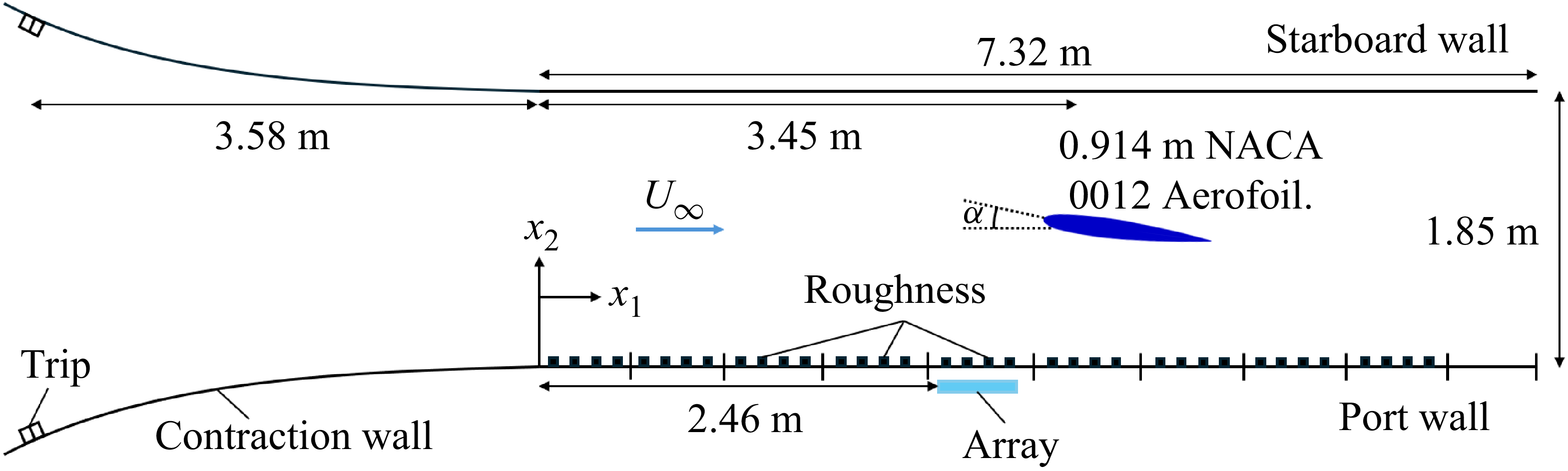


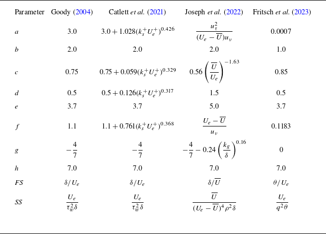
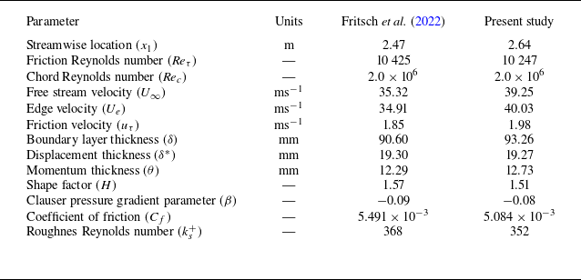


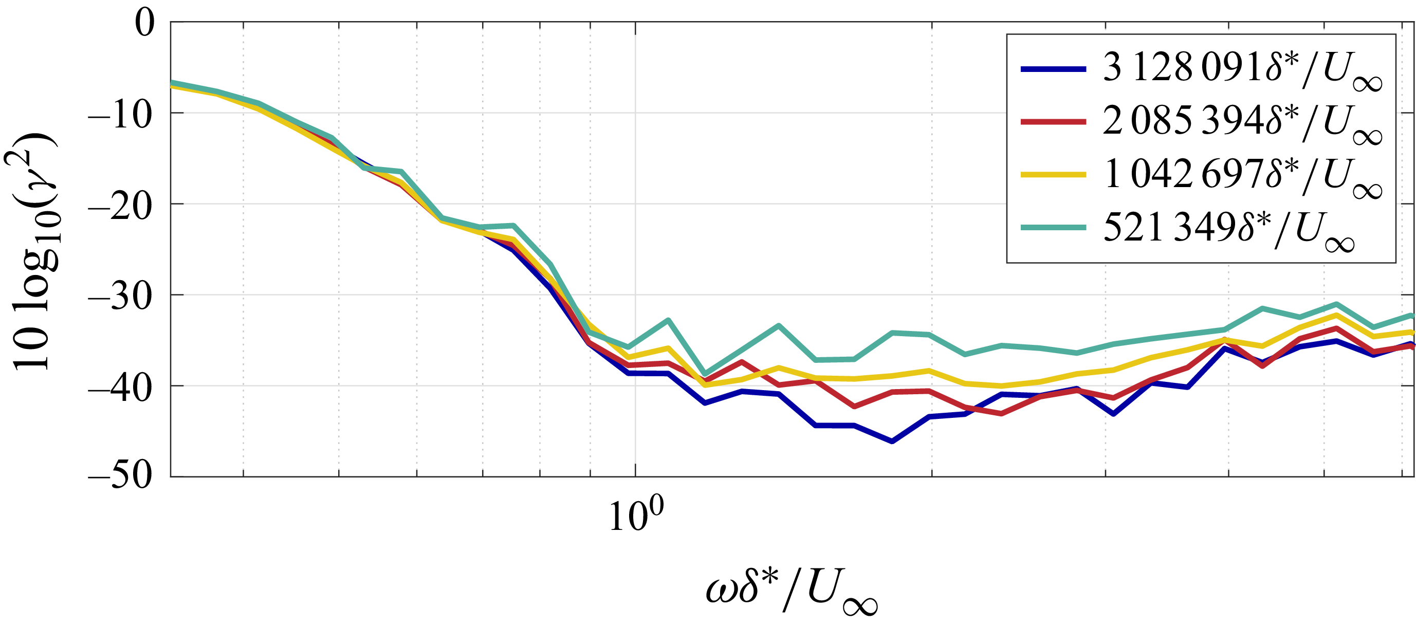


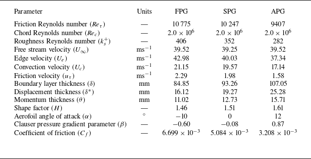


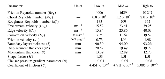


 Open access

