


1. Introduction
In a variety of applications, a deformable porous medium can be placed inside a confining container made of rigid and impermeable material. For example, this set-up is common in filtration experiments where filter cakes are housed in compression-permeability cells (Ruth Reference Ruth1935). This scenario is also encountered in geoengineering, where soil samples are consolidated in consolidation cells, and in medicine, particularly when a tumour develops within a confined environment (Delarue et al. Reference Delarue, Montel, Vignjevic, Prost, Joanny and Cappello2014). These porous media are then generally in contact with the confining structure, permitting the exertion of both normal and tangential forces between the two bodies.
The interaction between a porous medium and a confining structure has been widely studied, beginning with dry granular media where the permeating fluid (air) can be neglected. A key classical result is the Janssen effect (Janssen Reference Janssen1895; Sperl Reference Sperl2006), which arises in tall granular columns: due to interparticle interactions, vertical stresses are redirected laterally toward the container walls, where they are partially supported by friction. As a result, the vertical stress saturates exponentially with depth over a characteristic length $\lambda _{\mathcal{F}} = R/(2\mu K)$
, where
$\lambda _{\mathcal{F}} = R/(2\mu K)$
, where $R$
is the column radius,
$R$
is the column radius, $\mu$
is the coefficient of wall-grain friction and
$\mu$
is the coefficient of wall-grain friction and $K$
is the stress redirection coefficient, a dimensionless constant of order one analogous to the Poisson ratio for elastic solids. This modelling has been extended to liquid-saturated porous media, omitting the viscous pressure gradient induced by fluid flow (Taylor Reference Taylor1948; Aguilar-González et al. Reference Aguilar-González, Maza and Pacheco-Vázquez2025). Following this methodology, geotechnical investigations revealed that measured soil properties depend on the sample’s height
$K$
is the stress redirection coefficient, a dimensionless constant of order one analogous to the Poisson ratio for elastic solids. This modelling has been extended to liquid-saturated porous media, omitting the viscous pressure gradient induced by fluid flow (Taylor Reference Taylor1948; Aguilar-González et al. Reference Aguilar-González, Maza and Pacheco-Vázquez2025). Following this methodology, geotechnical investigations revealed that measured soil properties depend on the sample’s height $L$
relative to its radius
$L$
relative to its radius $R$
(Taylor Reference Taylor1948; Lovisa & Sivakugan Reference Lovisa and Sivakugan2015), leading to the standard practice in soil mechanics of limiting the ratio
$R$
(Taylor Reference Taylor1948; Lovisa & Sivakugan Reference Lovisa and Sivakugan2015), leading to the standard practice in soil mechanics of limiting the ratio $L/R$
to 0.8 (ASTM International 2004). In filtration applications, Lu, Huang & Hwang (Reference Lu, Huang and Hwang1998) incorporated wall friction through continuum modelling to refine predictions from compression-permeability cells, demonstrating that incorporating friction in the continuum model reduced the deviation between predictions and experiment by a factor of two. However, these studies typically simplify the interactions between frictional effects and fluid–solid interactions, either by ignoring the impact of viscous pressure gradients on the solid stresses (e.g. Lu et al. Reference Lu, Huang and Hwang1998) or by neglecting the impact of friction on the consolidation process (e.g. Lovisa & Sivakugan Reference Lovisa and Sivakugan2015). Moreover, they remain limited to monotonic loading and provide no insights into unloading or cyclic behaviour.
$L/R$
to 0.8 (ASTM International 2004). In filtration applications, Lu, Huang & Hwang (Reference Lu, Huang and Hwang1998) incorporated wall friction through continuum modelling to refine predictions from compression-permeability cells, demonstrating that incorporating friction in the continuum model reduced the deviation between predictions and experiment by a factor of two. However, these studies typically simplify the interactions between frictional effects and fluid–solid interactions, either by ignoring the impact of viscous pressure gradients on the solid stresses (e.g. Lu et al. Reference Lu, Huang and Hwang1998) or by neglecting the impact of friction on the consolidation process (e.g. Lovisa & Sivakugan Reference Lovisa and Sivakugan2015). Moreover, they remain limited to monotonic loading and provide no insights into unloading or cyclic behaviour.
A second approach has prioritised fluid–solid coupling while neglecting wall friction. For example, Beavers, Wilson & Masha (Reference Beavers, Wilson and Masha1975) documents an experiment where a polyurethane sponge is confined in a square channel and compressed by either a fluid flow or an external mechanical load, acting in the same way as a permeable piston. These authors observed poor agreement between experiment and modelling, which they attributed in part to the absence of friction in their model. Later, Parker, Mehta & Caro (Reference Parker, Mehta and Caro1987) and Lanir, Sauob & Maretsky (Reference Lanir, Sauob and Maretsky1990) conducted experiments using a sponge sample with a slightly reduced width compared with the dimensions of their experimental channel, thereby strategically mitigating the influence of wall friction. However, the resulting gap between the sponge and the walls allowed the flow to partially bypass the sponge, such that they could not simultaneously fit the volume flux and the deformation using a uniaxial theoretical model. More recently, Hewitt et al. (Reference Hewitt, Nijjer, Worster and Neufeld2016) conducted similar experiments on the packing of hydrogel beads. The authors derived a model to explain their experimental results, neglecting wall friction. The predictions agree with the compressive phase of their experiments, during which the applied pressure head is monotonically increased. However, the authors report unexpected hysteresis during decompression, both in the flow rate and macroscopic strain observed in their fluid-driven experiments and in mechanical stress–strain tests conducted separately. The authors associated this hysteresis with granular rearrangements rather than wall friction, in part because hydrogel beads are known to be particularly slippery (Cuccia et al. Reference Cuccia, Pothineni, Wu, Méndez Harper and Burton2020). This interpretation is consistent with previous studies on granular media, which reported extensive rearrangements in hydrogel packings (MacMinn, Dufresne & Wettlaufer Reference MacMinn, Dufresne and Wettlaufer2015). However, as explored in more detail below, wall friction can cause qualitatively similar hysteretic behaviour.
Two notable exceptions that bridge these two approaches are the work of Lutz (Lutz Reference Lutz2021; Lutz, Wilen & Wettlaufer Reference Lutz, Wilen and Wettlaufer2021) and Li (Li & Juanes Reference Li and Juanes2022). Lutz conducted experiments with a stack of latex foam discs in a cylindrical pipe. The foam discs were cut to match the cylinder’s inner diameter and the fluid pressure was measured at multiple locations within the porous medium. They conducted piston- and fluid-driven compression–decompression cycles and observed hysteresis in the displacement–pressure curves, which they attributed to wall friction. This wall friction was observed in both loading scenarios, and its relative importance was found to depend on the system’s aspect ratio. Importantly, they identified striking differences between piston-driven and fluid-driven scenarios: during fluid-driven cycles, the foam remained stuck throughout much of the decompression phase, whereas it slipped readily during piston-driven decompression. They developed a discrete model incorporating friction, which qualitatively reproduced their experimental observations. However, the absence of a continuum framework, combined with uncertainty in the size of their disks, limited the comparison between loading scenarios and their understanding of the fundamental poroelastic behaviour. Along similar lines, Li & Juanes (Reference Li and Juanes2022) used a novel photoporomechanical technique to visualise the effective stress field during classical poroelastic consolidation, highlighting the qualitative impact of wall friction and proposing a continuum model with a simplified friction term.
In summary, existing studies address two canonical scenarios, piston-driven and fluid-driven compression of a confined porous medium (figure 1), but fail to capture the full three-way coupling between solid deformation, interstitial fluid flow and wall friction. In piston-driven scenarios, cyclic loading remains undocumented and the mechanisms governing hysteresis and energy dissipation are poorly understood. In fluid-driven scenarios, no continuum framework exists to represent the frictional poroelastic response. Here, we study this three-way coupling theoretically. To do so, we develop a uniaxial poroelastic continuum model that accounts for Coulomb-like wall friction driven by stress redirection. We then focus our analysis on the quasistatic case, where the movements of the solid matrix are so slow that poroelastic transients can be neglected. This allows us to derive analytical expressions for the effective stress, the solid displacement and the energy dissipation during compression and decompression of a medium during loading by either a piston or a fluid flow. In the following, we present the general modelling framework in § 2 and the derivation of analytical solutions for quasistatic loading under a few simplifying assumptions in § 3.
A confined cylindrical porous medium is initially at rest (a) and is then compressed either by a permeable piston (b) or a fluid flow (c). The shading illustrates the level of stress experienced by the solid matrix in the absence of friction, in the steady state: the stress level is uniform in piston-driven compression and increases linearly from top to bottom in the fluid-driven compression (see § 3.1).

2. Modelling
2.1. Mechanical behaviour
2.1.1. Governing equations
In this paper we examine the interaction between friction and linear poroelasticity, leaving certain complexities of large deformation poromechanics for future work. In this section the key governing equations are briefly presented to describe the coupling of solid matrix deformation and fluid flow. The interested reader can find additional details in Coussy (Reference Coussy2004) and MacMinn, Dufresne & Wettlaufer (Reference MacMinn, Dufresne and Wettlaufer2016).
We assume that fluid flows through the medium according to Darcy’s law with an isotropic permeability $k$
, i.e.
$k$
, i.e.
 \begin{equation} \phi (\boldsymbol{v_{\!f}} - \boldsymbol{v_s}) = -\dfrac {k}{\eta } {\boldsymbol{\nabla }}\! P , \end{equation}
where $\phi$
is the porosity,
$\phi$
is the porosity, $\boldsymbol{v_{\!f}}$
is the velocity of the fluid (averaged over the fluid phase),
$\boldsymbol{v_{\!f}}$
is the velocity of the fluid (averaged over the fluid phase), $\boldsymbol{v_s}$
the solid velocity,
$\boldsymbol{v_s}$
the solid velocity, $\eta$
the fluid dynamic viscosity and
$\eta$
the fluid dynamic viscosity and $P$
the fluid pressure.
$P$
the fluid pressure.
Taking the fluid phase to be incompressible, mass conservation gives
 \begin{equation} \partial _t \phi + {\boldsymbol{\nabla }} \boldsymbol{\cdot }(\phi \boldsymbol{v_{\!f}})=0, \end{equation}
where $\partial _t$
is the partial derivative with respect to time.
$\partial _t$
is the partial derivative with respect to time.
Similarly, the solid phase is also assumed to be incompressible and mass conservation for the solid phase gives
 \begin{equation} -\partial _t \phi + {\boldsymbol{\nabla }} \boldsymbol{\cdot }\left ( (1-\phi ) \boldsymbol{v_s} \right )=0. \end{equation}
One can then define the total flux $\boldsymbol{q}$
as
$\boldsymbol{q}$
as
 \begin{equation} \boldsymbol{q} = \phi \boldsymbol{v_{\!f}} + (1-\phi ) \boldsymbol{v_s}, \end{equation}
and, from (2.2) and (2.3), it follows that
 \begin{equation} {\boldsymbol{\nabla }} \boldsymbol{\cdot }\boldsymbol{q} = 0. \end{equation}
The Terzaghi decomposition of stress is adopted (Terzaghi Reference Terzaghi1943), in which the total stress $\boldsymbol{\sigma }$
is equal to
$\boldsymbol{\sigma }$
is equal to
 \begin{equation} \boldsymbol{\sigma } = \boldsymbol{\sigma '} - P\! \unicode{x1D644}, \end{equation}
with $\boldsymbol{\sigma '}$
the Terzaghi effective stress (i.e. the component of the stress that deforms the solid) and
$\boldsymbol{\sigma '}$
the Terzaghi effective stress (i.e. the component of the stress that deforms the solid) and $\unicode{x1D644}$
the identity tensor, where the tension-positive sign convention from solid mechanics is adopted (François et al. Reference François, Pineau and Zaoui2012).
$\unicode{x1D644}$
the identity tensor, where the tension-positive sign convention from solid mechanics is adopted (François et al. Reference François, Pineau and Zaoui2012).
In the absence of inertia and gravity, mechanical equilibrium is given by
 \begin{equation} {\boldsymbol{\nabla }} \boldsymbol{\cdot }\boldsymbol{\sigma } = \boldsymbol{0}, \end{equation}
which, together with (2.6), implies that
 \begin{equation} {\boldsymbol{\nabla }} \boldsymbol{\cdot }\boldsymbol{\sigma ^\prime } = {\boldsymbol{\nabla }}\! P . \end{equation}
For simplicity, we now assume that the deformations of the solid matrix are small. However, we expect the physical reasoning and qualitative observations below to generalise readily to large deformations. In detail, if the solid matrix experiences a typical displacement of $u_s$
then the characteristic scale of the strain is
$u_s$
then the characteristic scale of the strain is $u_s/L_0$
, with
$u_s/L_0$
, with $L_0$
the typical relaxed length of the porous medium, and we assume that
$L_0$
the typical relaxed length of the porous medium, and we assume that $\left | u_s/L_0 \right | \ll 1$
. This assumption has four important consequences. First, the permeability is assumed to be constant and uniform. Second, the strain tensor
$\left | u_s/L_0 \right | \ll 1$
. This assumption has four important consequences. First, the permeability is assumed to be constant and uniform. Second, the strain tensor $\boldsymbol{\varepsilon }$
is related to the solid displacement
$\boldsymbol{\varepsilon }$
is related to the solid displacement $\boldsymbol{u_s}$
via
$\boldsymbol{u_s}$
via
 \begin{equation} \boldsymbol{\varepsilon } = \dfrac {1}{2} \left ( \boldsymbol{\nabla } \boldsymbol{u_s} + (\boldsymbol{\nabla } \boldsymbol{u_s} )^T \right )\!, \end{equation}
and the stress–strain relationship follows linear isotropic elasticity (e.g. François et al. Reference François, Pineau and Zaoui2012),
 \begin{equation} \boldsymbol{\sigma ^\prime } = (\mathcal{M}-\lambda ) \boldsymbol{\varepsilon } + \lambda \text{Tr} (\boldsymbol{\varepsilon }) \unicode{x1D644}, \end{equation}
where $\mathcal{M}$
and
$\mathcal{M}$
and $\lambda$
are the oedometric modulus and the first Lamé coefficient, respectively. Third, the porosity is related to the solid displacement via (e.g. MacMinn et al. Reference MacMinn, Dufresne and Wettlaufer2016)
$\lambda$
are the oedometric modulus and the first Lamé coefficient, respectively. Third, the porosity is related to the solid displacement via (e.g. MacMinn et al. Reference MacMinn, Dufresne and Wettlaufer2016)
 \begin{equation} \boldsymbol{{\nabla }}\boldsymbol{\cdot }\boldsymbol{u_s} = \dfrac {\phi -\phi _0}{1-\phi _0}, \end{equation}
with $\phi _0$
the uniform relaxed porosity. Fourth, the solid velocity is related to the solid displacement via
$\phi _0$
the uniform relaxed porosity. Fourth, the solid velocity is related to the solid displacement via $v_s = \partial {u_s}/\partial {t}$
, such that
$v_s = \partial {u_s}/\partial {t}$
, such that
 \begin{equation} {\boldsymbol{\nabla }} \boldsymbol{\cdot }\boldsymbol{v_s} = {\boldsymbol{\nabla }} \boldsymbol{\cdot }(\partial _t\boldsymbol{u_s}) = \partial _t \big( {\boldsymbol{\nabla }} \boldsymbol{\cdot }\boldsymbol{u_s} \big ). \end{equation}
Combining (2.1) and (2.4) with (2.5) gives
 \begin{equation} {\boldsymbol{\nabla }}\boldsymbol{\cdot }\boldsymbol{v_s} - {\boldsymbol{\nabla }}\boldsymbol{\cdot }\left (\frac {k}{\eta } {\boldsymbol{\nabla }}\! P\right ) = 0. \end{equation}
Using (2.11) and (2.12), (2.13) becomes
 \begin{equation} \frac {\partial _t \phi }{1-\phi _0} - \frac {k}{\eta } {\boldsymbol{\nabla }} \boldsymbol{\cdot } \big({\boldsymbol{\nabla }}\! P \big) = 0, \end{equation}
which is one form of the classical linear poroelastic flow equation. Neglecting frictional effects, (2.14) can be written in the form of a linear diffusion equation for the porosity field: the fluid pressure is coupled to the effective stress via (2.8) and the porosity is coupled to the solid mechanics via (2.9) and (2.10). This is the classical poroelasticity theory for incompressible constituents (Coussy Reference Coussy2004).
2.1.2. Boundary conditions, initial values
We consider a porous medium of relaxed length $L_0$
confined within a cylindrical structure of radius
$L_0$
confined within a cylindrical structure of radius $R$
(figure 1
a), which undergoes uniaxial compression. In the following, we adopt cylindrical coordinates (
$R$
(figure 1
a), which undergoes uniaxial compression. In the following, we adopt cylindrical coordinates ( $\boldsymbol{e_r},\boldsymbol{e_\theta },\boldsymbol{e_z}$
), as illustrated in figure 1. As the confining structure is impermeable to both fluid and solid,
$\boldsymbol{e_r},\boldsymbol{e_\theta },\boldsymbol{e_z}$
), as illustrated in figure 1. As the confining structure is impermeable to both fluid and solid,
 \begin{equation} \left . \boldsymbol{v_s}\boldsymbol{\cdot }\boldsymbol{e_r} \right |_R =\left . \boldsymbol{v_{\!f}}\boldsymbol{\cdot }\boldsymbol{e_r}\right |_R = 0, \end{equation}
where $ \boldsymbol{v_s}\boldsymbol{\cdot }\boldsymbol{e_r} |_R$
and
$ \boldsymbol{v_s}\boldsymbol{\cdot }\boldsymbol{e_r} |_R$
and $\boldsymbol{v_{\!f}}\boldsymbol{\cdot }\boldsymbol{e_r} |_R$
are, respectively, the solid and fluid velocity normal to the walls.
$\boldsymbol{v_{\!f}}\boldsymbol{\cdot }\boldsymbol{e_r} |_R$
are, respectively, the solid and fluid velocity normal to the walls.
For downward piston-driven compression, we take the top boundary to be permeable such that the effective stress is equal to the stress applied by the piston and the fluid pressure is null. We take the piston to be controlled in loading and, for simplicity, we take the imposed stress to be uniform over the top boundary (as in Hewitt et al. Reference Hewitt, Nijjer, Worster and Neufeld2016; MacMinn et al. Reference MacMinn, Dufresne and Wettlaufer2016). Finally, we take the bottom boundary to be permeable and fixed in place, such that the solid displacement and the fluid pressure are null. Thus, we have
 \begin{equation} \left \{ \begin{array}{lll}\!\! \sigma _{zz}^{\prime } = -\sigma ^{\prime \star } & \text{and } P = 0 \ \mathrm{at} \ z=L, \\[9pt] \!\! \boldsymbol{u_s}= \boldsymbol{0} & \text{and } P = 0 \ \mathrm{at} \ z=0, \end{array}\right . \end{equation}
where the location $z=L\approx L_0$
represents the top of the medium and
$z=L\approx L_0$
represents the top of the medium and $z=0$
the bottom of the medium, and where
$z=0$
the bottom of the medium, and where $-\sigma ^{\prime \star }$
is the stress applied by the piston, with
$-\sigma ^{\prime \star }$
is the stress applied by the piston, with $\sigma ^{\prime \star }\gt 0$
.
$\sigma ^{\prime \star }\gt 0$
.
For downward fluid-driven compression, we take the top boundary to be unconstrained, so that the associated mechanical stress is null and the fluid pressure is equal to the imposed operating pressure $\Delta P^\star$
. We take the bottom boundary to be again permeable and fixed in place, such that the solid displacement and the fluid pressure are again null. Thus, we have
$\Delta P^\star$
. We take the bottom boundary to be again permeable and fixed in place, such that the solid displacement and the fluid pressure are again null. Thus, we have
 \begin{equation} \left \{ \begin{array}{lll}\!\! \sigma _{zz}^{\prime } = 0 & \text{and } P = \Delta P^\star \ \text{at } \ z=L ,\\[9pt] \!\! \boldsymbol{u_s} = \boldsymbol{0} & \text{and } P = 0 \ \text{at } \ z=0 .\end{array}\right . \end{equation}
2.2. Impact of friction
2.2.1. Modelling tangential forces and confinement
In this problem, friction manifests as a non-zero shear stress between the material and the confining walls, $\sigma '_{rz}(r=R) \neq 0$
. We next consider the impact of friction on the two problems above.
$\sigma '_{rz}(r=R) \neq 0$
. We next consider the impact of friction on the two problems above.
Because of the axisymmetry, all quantities remain constant along with varying $\theta$
. Furthermore, the uniaxial nature of the problem suggests that
$\theta$
. Furthermore, the uniaxial nature of the problem suggests that $u_s$
,
$u_s$
, $v_s$
and
$v_s$
and $v_{\!f}$
will be primarily directed along
$v_{\!f}$
will be primarily directed along $\boldsymbol{e_z}$
, such that
$\boldsymbol{e_z}$
, such that $\boldsymbol{v_{\!f}} \approx {} v_{\!f}(r,z) \boldsymbol{e_z},\, \boldsymbol{v_s} \approx {} v_s(r,z) \boldsymbol{e_z}$
and
$\boldsymbol{v_{\!f}} \approx {} v_{\!f}(r,z) \boldsymbol{e_z},\, \boldsymbol{v_s} \approx {} v_s(r,z) \boldsymbol{e_z}$
and $\boldsymbol{u_s} \approx u_s(r,z) \boldsymbol{e_z}$
. From (2.9), the strain is then
$\boldsymbol{u_s} \approx u_s(r,z) \boldsymbol{e_z}$
. From (2.9), the strain is then
 \begin{equation} \boldsymbol{\varepsilon } = \begin{pmatrix} 0 & 0 & \dfrac {1}{2} \partial _r u_s \\[9pt] 0 & 0 & 0 \\[9pt] \dfrac {1}{2} \partial _r u_s & 0 & \partial _z u_s \end{pmatrix}\! , \end{equation}
so that (2.11) implies that
 \begin{equation} \varepsilon _{zz} = \dfrac {\phi -\phi _0}{1-\phi _0}. \end{equation}
From (2.10) and (2.18), the effective stress is then
 \begin{equation} \boldsymbol{\sigma ^\prime } = \begin{pmatrix} \lambda \varepsilon _{zz} & 0 & (\mathcal{M}-\lambda ) \varepsilon _{rz} \\[5pt] 0 & \lambda \varepsilon _{zz} & 0 \\[5pt] (\mathcal{M}-\lambda ) \varepsilon _{rz} & 0 & \mathcal{M} \varepsilon _{zz} \end{pmatrix}\! . \end{equation}
Therefore, the $z$
component of (2.8) becomes
$z$
component of (2.8) becomes
 \begin{equation} \partial _z \sigma ^\prime _{zz} + \frac {\partial _r \left (r\sigma ^\prime _{rz}\right )}{r} = \partial _z P. \end{equation}
Equation (2.21) can be integrated along $r$
and
$r$
and $\theta$
:
$\theta$
:
 \begin{equation} \int _0^R \int _0^{2\pi } \left (r \partial _z \sigma ^\prime _{zz} + \partial _r (r \sigma ^\prime _{rz}) \right ) {\rm d}r{\rm d}\theta = \int _0^R \int _0^{2\pi } \partial _z P r{\rm d}r{\rm d}\theta . \end{equation}
This result is then simplified as follows. First, as mentioned in § 2.1.2, we aim to capture mechanical tests and other scenarios that are restricted to compression of the medium, rather than shear mechanics. Therefore, we assume that $\sigma ^\prime _{zz}$
is constant over horizontal cross-sections, as is usually done in the classical Janssen modelling:
$\sigma ^\prime _{zz}$
is constant over horizontal cross-sections, as is usually done in the classical Janssen modelling:
 \begin{equation} \int _0^R \int _0^{2\pi } r\partial _z \sigma ^\prime _{zz} {\rm d}r{\rm d}\theta = \pi R^2 \partial _z \sigma _{zz}^\prime . \end{equation}
Second, the $r$
component of Darcy’s law (2.1) implies that
$r$
component of Darcy’s law (2.1) implies that $\partial _r P = 0$
and, as a result, that
$\partial _r P = 0$
and, as a result, that
 \begin{equation} \int _0^R \int _0^{2\pi } \partial _z P r{\rm d}r{\rm d}\theta = \pi R^2 \partial _z P. \end{equation}
Third, one may note that
 \begin{equation} \int _0^{2\pi } \int _0^R \partial _r (r \sigma ^\prime _{rz}){\rm d}r{\rm d}\theta = 2 \pi [r \sigma ^\prime _{rz}]_0^R = 2\pi R \left . \sigma ^\prime _{rz} \right |_R, \end{equation}
where the term $\sigma ^\prime _{rz} \rvert _R$
is the frictional stress applied by the wall on the solid matrix, which, going forward, we denote as
$\sigma ^\prime _{rz} \rvert _R$
is the frictional stress applied by the wall on the solid matrix, which, going forward, we denote as $\sigma ^\prime _{\mathcal{F}}$
. Using (2.23)–(2.25), (2.22) reduces to
$\sigma ^\prime _{\mathcal{F}}$
. Using (2.23)–(2.25), (2.22) reduces to
 \begin{equation} \partial _z \sigma ^\prime _{zz} + \dfrac {2 {\sigma }^\prime _{\mathcal{F}}}{R} = \partial _zP . \end{equation}
Note that this result was derived assuming uniform $\sigma ^\prime _{zz}$
across horizontal sections. More generally, the term
$\sigma ^\prime _{zz}$
across horizontal sections. More generally, the term $\partial _z \sigma ^\prime _{zz}$
can be interpreted as the cross-sectional average defined in (2.23), allowing this formulation to be extended beyond the uniform stress assumption.
$\partial _z \sigma ^\prime _{zz}$
can be interpreted as the cross-sectional average defined in (2.23), allowing this formulation to be extended beyond the uniform stress assumption.
In the following, we explore how a non-zero frictional stress $\sigma ^\prime _{\mathcal{F}}$
modifies the coupling between the solid stress and the fluid pressure.
$\sigma ^\prime _{\mathcal{F}}$
modifies the coupling between the solid stress and the fluid pressure.
2.2.2. Modelling of friction and stress redirection
The simplest way to model wall friction is via Coulomb’s law (Ludema Reference Ludema1996). Coulomb’s law states that the friction force between two solid bodies in contact opposes the relative motion of the bodies, up to a maximum value proportional to the normal load. The associated constant of proportionality is called the coefficient of friction. Coulomb’s law further postulates that this coefficient does not depend on the area of contact or the speed of relative motion. However, it may depend on the existence of relative motion – a distinction being made between the static coefficient, when the relative speed is null, and the dynamic coefficient, when the relative velocity is non-zero. We take the static and dynamic values to be equal for simplicity, and thus, write Coulomb’s law as
 \begin{equation} \begin{cases} \sigma _F^\prime = \mathrm{sgn}(v_s) \mu \, \sigma ^\prime _{rr} & \iff \left | v_s \right | \gt 0, \\[5pt] \left | \sigma _F^\prime \right | \leqslant \mu \left | \sigma ^\prime _{rr} \right | & \iff v_s = 0 , \end{cases} \end{equation}
with $\mu$
the (dimensionless) coefficient of friction and
$\mu$
the (dimensionless) coefficient of friction and $\mathrm{sgn}(v_s)$
the sign of
$\mathrm{sgn}(v_s)$
the sign of $v_s$
. This law is restricted to situations where the normal load is null or pushing on the wall (
$v_s$
. This law is restricted to situations where the normal load is null or pushing on the wall ( $\sigma '_{rr}(R) \leqslant 0$
). The case where a tangential force is not null in the presence of pulling forces (
$\sigma '_{rr}(R) \leqslant 0$
). The case where a tangential force is not null in the presence of pulling forces ( $\sigma '_{rr} (R) \gt 0$
) corresponds to an adhesive surface and will not be discussed in this study.
$\sigma '_{rr} (R) \gt 0$
) corresponds to an adhesive surface and will not be discussed in this study.
The link between $\sigma _{rr}^\prime$
and
$\sigma _{rr}^\prime$
and $\sigma _{zz}^\prime$
can be made in two ways. The first way is through linear elasticity, where (2.20) states that
$\sigma _{zz}^\prime$
can be made in two ways. The first way is through linear elasticity, where (2.20) states that $\sigma ^\prime _{rr}\,=\,[\nu /(1-\nu )]\sigma _{zz}^{\prime }$
, with
$\sigma ^\prime _{rr}\,=\,[\nu /(1-\nu )]\sigma _{zz}^{\prime }$
, with $\nu$
the Poisson ratio of the solid skeleton. The second way is via the mechanics of granular media, where materials are not simple elastic solids and do not obey linear elasticity. Nonetheless, a classical assumption in granular media is that the vertical stress is redirected in the horizontal direction in a fixed proportion:
$\nu$
the Poisson ratio of the solid skeleton. The second way is via the mechanics of granular media, where materials are not simple elastic solids and do not obey linear elasticity. Nonetheless, a classical assumption in granular media is that the vertical stress is redirected in the horizontal direction in a fixed proportion: $\sigma ^\prime _{rr} = K \sigma ^\prime _{zz}$
, with
$\sigma ^\prime _{rr} = K \sigma ^\prime _{zz}$
, with $K$
a dimensionless constant, sometimes referred to as the Janssen parameter (e.g. Ovarlez & Clément Reference Ovarlez and Clément2005). Although not derived from linear elasticity, this relation qualitatively resembles the stress redistribution observed in elastic solids, with
$K$
a dimensionless constant, sometimes referred to as the Janssen parameter (e.g. Ovarlez & Clément Reference Ovarlez and Clément2005). Although not derived from linear elasticity, this relation qualitatively resembles the stress redistribution observed in elastic solids, with $K$
playing the same role as
$K$
playing the same role as ${\nu }/({1-\nu })$
, and thus,
${\nu }/({1-\nu })$
, and thus, $K\approx 1$
for incompressible materials. Applying the convention from granular materials, (2.27) becomes
$K\approx 1$
for incompressible materials. Applying the convention from granular materials, (2.27) becomes
 \begin{equation} \begin{cases} \sigma _F^\prime = \mathrm{sgn}(v_s) \mu K \sigma ^\prime _{zz} & \iff \left | v_s \right | \gt 0, \\[5pt] \left | \sigma _F^\prime \right | \leqslant \mu K \left | \sigma ^\prime _{zz} \right | & \iff v_s = 0 . \end{cases} \end{equation}
With (2.28), the model is fully specified (i.e. this system of equations is closed). Note that (2.28) does not determine the value of $\sigma ^\prime _{\mathcal{F}}$
in the case
$\sigma ^\prime _{\mathcal{F}}$
in the case $v_s=0$
, but the fact that
$v_s=0$
, but the fact that $v_s=0$
provides sufficient information to determine
$v_s=0$
provides sufficient information to determine $\sigma ^\prime _{\mathcal{F}}$
from the other parts of the model – for example, see (A2) in Appendix A. Because many intermediate equations were detailed here, we summarise the equations to be solved in table 1, comprising a system of eight independent equations with eight unknown variables.
$\sigma ^\prime _{\mathcal{F}}$
from the other parts of the model – for example, see (A2) in Appendix A. Because many intermediate equations were detailed here, we summarise the equations to be solved in table 1, comprising a system of eight independent equations with eight unknown variables.
Summary of the model. Each independent equation is displayed (middle column) with its number for easier reference in text (right column) and a short name (left column). The system comprises eight independent equations with eight unknown variables: $\phi , v_f, v_s, q, P, \varepsilon _{zz}, \sigma _{zz}^\prime$
and
$\phi , v_f, v_s, q, P, \varepsilon _{zz}, \sigma _{zz}^\prime$
and $ \sigma _F^\prime$
. The other quantities,
$ \sigma _F^\prime$
. The other quantities, $k$
,
$k$
, $\eta$
,
$\eta$
, $\mathcal{M}$
,
$\mathcal{M}$
, $\phi _0$
,
$\phi _0$
, $R$
,
$R$
, $\mu$
and
$\mu$
and $K$
, are constant parameters, assumed to be known.
$K$
, are constant parameters, assumed to be known.

2.3. Sliding regime
The model presented in table 1 is generally intractable to solve analytically. Indeed, $\sigma '_F (z)$
may exhibit discontinuities due to the distinction between stick and slip (
$\sigma '_F (z)$
may exhibit discontinuities due to the distinction between stick and slip ( $v_s=0$
versus
$v_s=0$
versus $|v_s|\gt 0$
) and its sign depends on the sign of
$|v_s|\gt 0$
) and its sign depends on the sign of $v_s$
. These complications can be substantially simplified by considering, for example, an initially uncompressed medium subjected to a monotonically increasing fluid pressure
$v_s$
. These complications can be substantially simplified by considering, for example, an initially uncompressed medium subjected to a monotonically increasing fluid pressure $\Delta \tilde P^{\star }$
or mechanical load
$\Delta \tilde P^{\star }$
or mechanical load $\tilde \sigma ^{\prime \star }$
. In this scenario, the entire medium undergoes compression (
$\tilde \sigma ^{\prime \star }$
. In this scenario, the entire medium undergoes compression ( $v_s\lt 0$
for
$v_s\lt 0$
for $z\in [0,L]$
), and the magnitude of the friction stress everywhere equals its maximum value:
$z\in [0,L]$
), and the magnitude of the friction stress everywhere equals its maximum value:
 \begin{equation} \left | \sigma _F^\prime \right | = \mu K \left | \sigma _{zz}^{\prime } \right | . \end{equation}
This framework extends to arbitrary loading scenarios by analysing individual sliding regions, defined as domains where $|v_s| \gt 0$
. Within such a region, the continuity of
$|v_s| \gt 0$
. Within such a region, the continuity of $v_s$
ensures that it remains uniformly positive or negative. In that case, (2.29) remains valid throughout the entire sliding region and (2.26) reduces to
$v_s$
ensures that it remains uniformly positive or negative. In that case, (2.29) remains valid throughout the entire sliding region and (2.26) reduces to
 \begin{equation} \partial _z P = \partial _z \sigma _{zz}^{\prime } +\mathrm{sgn}(v_s) 2 \dfrac {\mu K}{R} \sigma _{zz}^{\prime }, \end{equation}
where $\mathrm{sgn}(v_s)=-1$
when the solid moves downward (e.g. during compression) and
$\mathrm{sgn}(v_s)=-1$
when the solid moves downward (e.g. during compression) and $\mathrm{sgn}(v_s)=1$
when it moves upward (e.g. during decompression).
$\mathrm{sgn}(v_s)=1$
when it moves upward (e.g. during decompression).
Applying the porosity–strain relationship (2.19), and linear elasticity (2.20), to (2.14) leads to
 \begin{equation} \partial ^2_{z} P = \frac {\eta }{k \mathcal{M}}\partial _t \sigma _{zz}^{\prime }. \end{equation}
Differentiating (2.30) with respect to $z$
and substituting into (2.31) leads to
$z$
and substituting into (2.31) leads to
 \begin{equation} \partial _t \sigma _{zz}^{\prime } = \frac {k\mathcal{M}}{\eta } \partial ^2_z \sigma _{zz}^{\prime } + \mathrm{sgn}(v_s) \frac {k\mathcal{M}}{\eta }\frac {2 \mu K}{R} \partial _z \sigma _{zz}^{\prime }. \end{equation}
This linear parabolic partial differential equation describes the evolution of the effective stress during the sliding of a confined porous medium. Equation (2.32) has the structure of a diffusion–advection equation, with the diffusion term being poroelastic (first term on the right-hand side) and the advection term being frictional (second term on the right-hand side).
2.4. Scaling
In the following, (2.32) and the set of equations presented in table 1 are scaled as
 \begin{equation} \begin{aligned} \tilde {z} = \dfrac {z}{L}, & \quad \tilde {u}_s = \dfrac {u_s}{L}, & \tilde {t} = \frac {t}{T_{\textit{pe}}}, \\ \quad \tilde {\sigma }^\prime = \dfrac {\sigma _{zz}^{\prime }}{\mathcal{M}}, & \quad \tilde {P} = \dfrac {P}{\mathcal{M}}, \end{aligned} \end{equation}
where we used tildes to indicate non-dimensional variables, simplified the notation, writing $\tilde {\sigma }^\prime := \tilde {\sigma }^\prime _{zz}$
, as this is the only component of the stress tensor that appears in the remainder of the paper, and where
$\tilde {\sigma }^\prime := \tilde {\sigma }^\prime _{zz}$
, as this is the only component of the stress tensor that appears in the remainder of the paper, and where
 \begin{equation} T_{\textit{pe}}=\frac {\eta L^2}{k\mathcal{M}} \end{equation}
is the classical poroelastic time scale (Cheng Reference Cheng2016). With these scalings, (2.32) can be written in non-dimensional form as
 \begin{equation} \partial _{\tilde {t}} \tilde {\sigma }^\prime = \partial ^2_{\tilde {z}} \tilde {\sigma }^\prime + \mathrm{sgn}(v_s) \frac {2 \mu \textit{KL}}{R} \partial _{\tilde {z}} \tilde {\sigma }^\prime . \end{equation}
This equation shows that during the sliding of a frictional porous medium, the analogue of the Péclet number is the dimensionless number
 \begin{equation} {\mathcal{F}} = \dfrac {2\mu \textit{KL}}{R}, \end{equation}
which we name the ‘friction number’ (see also Li & Juanes Reference Li and Juanes2022). Equation (2.30) can then be written in non-dimensional form as
 \begin{equation} \partial _{\tilde {z}} \tilde {P} = \partial _{\tilde {z}} \tilde {\sigma }^\prime + \mathrm{sgn}(v_s) {\mathcal{F}} \tilde {\sigma }^\prime . \end{equation}
This equation shows that $\mathcal{F}$
represents the importance of friction in mechanical equilibrium relative to the other terms of (2.37). For
$\mathcal{F}$
represents the importance of friction in mechanical equilibrium relative to the other terms of (2.37). For ${\mathcal{F}} \ll 1$
, friction is negligible and the gradients in fluid pressure and effective stress are fully coupled (
${\mathcal{F}} \ll 1$
, friction is negligible and the gradients in fluid pressure and effective stress are fully coupled ( $\partial _{\tilde {z}} \tilde {P} \approx \partial _{\tilde {z}} \tilde {\sigma }^\prime$
), such that any variation of fluid pressure is transmitted to the solid. However, for
$\partial _{\tilde {z}} \tilde {P} \approx \partial _{\tilde {z}} \tilde {\sigma }^\prime$
), such that any variation of fluid pressure is transmitted to the solid. However, for ${\mathcal{F}} \gtrsim 1$
, fluid pressure gradients are balanced by a combination of solid stress gradients and the frictional contribution due to
${\mathcal{F}} \gtrsim 1$
, fluid pressure gradients are balanced by a combination of solid stress gradients and the frictional contribution due to $\sigma _F^\prime$
. Note that
$\sigma _F^\prime$
. Note that $\mathcal{F}$
is proportional to the coefficient of friction (
$\mathcal{F}$
is proportional to the coefficient of friction ( $\mu$
), the coefficient of stress redirection (
$\mu$
), the coefficient of stress redirection ( $K$
) and the aspect ratio of the porous medium (
$K$
) and the aspect ratio of the porous medium ( $L/R$
). Therefore, friction may have significant effects even with a low coefficient of friction, as long as the medium is strongly confined (i.e. if the aspect ratio is high).
$L/R$
). Therefore, friction may have significant effects even with a low coefficient of friction, as long as the medium is strongly confined (i.e. if the aspect ratio is high).
For quasistatic loading (i.e. loading that is slow relative to the poroelastic time scale), our problem reduces to a steady advection–diffusion problem. Indeed, in (2.35) the time can be non-dimensionalised by the loading time scale $T_{\textit{load}}$
instead of the poroelastic time scale, which leads to
$T_{\textit{load}}$
instead of the poroelastic time scale, which leads to
 \begin{equation} \frac {T_{\textit{pe}}}{T_{\textit{load}}}\partial _{\tilde {t}} \tilde {\sigma }^\prime = \partial ^2_{\tilde {z}} \tilde {\sigma }^\prime + \mathrm{sgn}(v_s) {\mathcal{F}} \partial _{\tilde {z}} \tilde {\sigma }^\prime , \end{equation}
so that, for sufficiently high $T_{\textit{load}}$
,
$T_{\textit{load}}$
, $({T_{\textit{pe}}}/{T_{\textit{load}}})\partial _{\tilde {t}} \tilde {\sigma }^\prime \ll 1$
and the left-hand term can be neglected. In this case, integrating (2.38) with respect to
$({T_{\textit{pe}}}/{T_{\textit{load}}})\partial _{\tilde {t}} \tilde {\sigma }^\prime \ll 1$
and the left-hand term can be neglected. In this case, integrating (2.38) with respect to $\tilde {z}$
leads to
$\tilde {z}$
leads to
 \begin{equation} C= \partial _{\tilde {z}} \tilde {\sigma }^\prime + \mathrm{sgn}(v_s) {\mathcal{F}} \tilde {\sigma }^\prime , \end{equation}
where $C$
is a constant that we identify as
$C$
is a constant that we identify as $\partial _z \tilde {P}$
, using (2.37). Therefore, for quasistatic loadings, (2.37) can be solved as a differential equation in
$\partial _z \tilde {P}$
, using (2.37). Therefore, for quasistatic loadings, (2.37) can be solved as a differential equation in $\tilde {\sigma }^\prime$
and its spatial derivatives along the
$\tilde {\sigma }^\prime$
and its spatial derivatives along the $\tilde {z}$
coordinate.
$\tilde {z}$
coordinate.
Finally, note that the modelling and results presented here are readily generalised to any geometry with a uniform horizontal cross-section (along the $z$
direction), i.e.
$z$
direction), i.e.
 \begin{equation} {\mathcal{F}} = \mu \textit{KL} \frac {\mathcal{P}}{\mathcal{A}}, \end{equation}
where $\mathcal{P}$
represents the perimeter of a cross-section and
$\mathcal{P}$
represents the perimeter of a cross-section and $\mathcal{A}$
its area. This ratio reduces to
$\mathcal{A}$
its area. This ratio reduces to $2/R$
for a cylindrical structure, to
$2/R$
for a cylindrical structure, to $2(H+W)/(HW)$
for a rectangular cross-section of width
$2(H+W)/(HW)$
for a rectangular cross-section of width $W$
and height
$W$
and height $H$
and to
$H$
and to $2/W$
for slender structures (
$2/W$
for slender structures ( $H \gg W$
).
$H \gg W$
).
3. Results
3.1. Results in the absence of friction
In the following, we focus on the quasistatic regime and work in terms of dimensionless quantities. In the absence of friction ${\mathcal{F}}=0$
and (2.37) reduces to
${\mathcal{F}}=0$
and (2.37) reduces to
 \begin{equation} \partial _{{\tilde {z}}} \tilde {P} = \partial _{{\tilde {z}}} \tilde {\sigma }^\prime . \end{equation}
The quasistatic compression driven by a piston (i.e. so-called ‘drained’ compression) is conceptually the simplest case. Our assumptions imply that the fluid has time to exit the porous medium so that viscous pressure gradients are negligible ( $\partial _{{\tilde {z}}}\tilde {P}=0$
), in which case the problem is simply elastic rather than poroelastic. In this case, the effective stress is uniform and equal to the imposed stress (figure 1
b), i.e.
$\partial _{{\tilde {z}}}\tilde {P}=0$
), in which case the problem is simply elastic rather than poroelastic. In this case, the effective stress is uniform and equal to the imposed stress (figure 1
b), i.e.
 \begin{equation} \tilde {\sigma }^\prime = -\tilde \sigma ^{\prime \star }, \end{equation}
and the displacement field is linear in $\tilde {z}$
:
$\tilde {z}$
:
 \begin{equation} \tilde {u_s}= -{\tilde \sigma ^{\prime \star }}{\tilde {z}}. \end{equation}
For quasistatic compression by a fluid flow, in contrast, the effective stress increases linearly from the top to the bottom, due to the uniform gradient of fluid pressure (figure 1 c), i.e.
 \begin{equation} \tilde {\sigma }^\prime = - \Delta \tilde P^{\star }\left (1 -{\tilde {z}} \right ), \end{equation}
so that the displacement field is quadratic in $\tilde {z}$
:
$\tilde {z}$
:
 \begin{equation} \tilde {u_s}= -\Delta \tilde P^{\star } \, {\tilde {z}}\left ( 1- \frac {{\tilde {z}}}{2} \right )\!. \end{equation}
3.2. Solutions during compression
We now consider the frictional case under compression. An initially uncompressed medium is subjected to compression by steadily increasing the mechanical forcing. Under these conditions, sliding occurs throughout the entire medium, meaning (2.37) is valid everywhere within the domain.
When compression is driven by a piston, (2.37) simplifies to
 \begin{equation} 0 = \partial _{{\tilde {z}}} {\tilde {\sigma }^\prime } - {{\mathcal{F}}} {\tilde {\sigma }^\prime }. \end{equation}
In this case, the solution of (3.6) is
 \begin{equation} {\tilde \sigma ^{\prime }} = -{\tilde \sigma ^{\prime \star }} \exp \left [{ -{\mathcal{F}} \left (1-{\tilde {z}} \right )} \right ]\!. \end{equation}
The displacement field $\tilde {u}_s$
is then obtained by integrating the strain, directly computed from the stress–strain relationship (2.20), over the
$\tilde {u}_s$
is then obtained by integrating the strain, directly computed from the stress–strain relationship (2.20), over the $\tilde {z}$
coordinate, and imposing
$\tilde {z}$
coordinate, and imposing ${\tilde {u}_s} |_{{\tilde {z}}=0}=0$
:
${\tilde {u}_s} |_{{\tilde {z}}=0}=0$
:
 \begin{equation} {\tilde {u}_s} = -\dfrac {\tilde \sigma ^{\prime \star }}{ {\mathcal{F}}} \left \{ \exp \left [{- {\mathcal{F}} \left (1-{\tilde {z}} \right )}\right ]-\exp ({-{\mathcal{F}}}) \right \}\! . \end{equation}
In the case of a fluid-driven compression, the pressure difference across the medium $\Delta \tilde {P}^{\star }$
is imposed, while the effective stress at the top is zero. Therefore, (2.30) may be rewritten by replacing
$\Delta \tilde {P}^{\star }$
is imposed, while the effective stress at the top is zero. Therefore, (2.30) may be rewritten by replacing $\partial _{{\tilde {z}}} \tilde {P} = \Delta \tilde {P}^{\star }$
:
$\partial _{{\tilde {z}}} \tilde {P} = \Delta \tilde {P}^{\star }$
:
 \begin{equation} \Delta \tilde {P}^\star = \partial _{{\tilde {z}}} \tilde \sigma ^{\prime } - {\mathcal{F}} \tilde \sigma ^{\prime } . \end{equation}
With the boundary condition $\sigma ^{\prime } |_{{\tilde {z}}=1} = 0$
, the solution is
$\sigma ^{\prime } |_{{\tilde {z}}=1} = 0$
, the solution is
 \begin{equation} \tilde \sigma ^{\prime } = -\dfrac {\Delta \tilde {P}^\star }{{\mathcal{F}}} \left \{1- \exp \left [-{\mathcal{F}}\left (1-{\tilde {z}} \right )\right ] \right \}\!. \end{equation}
The displacement field is obtained as before:
 \begin{equation} \tilde {u}_s = -\dfrac {\Delta \tilde {P}^\star }{ {\mathcal{F}}^2} \left \{ {\mathcal{F}}{\tilde {z}}+\exp ({ -{\mathcal{F}}}) -\exp \left [ -{\mathcal{F}} \left (1- {\tilde {z}} \right ) \right ] \right \}\!. \end{equation}
Magnitude of the effective stress (top row) and of the relative displacements (bottom row), as a function of relative position ( $\tilde {z}$
), due to forcing by a piston (a and d, (3.7) and (3.8)) or by a fluid flow (b and e, (3.10) and (3.11)), with
$\tilde {z}$
), due to forcing by a piston (a and d, (3.7) and (3.8)) or by a fluid flow (b and e, (3.10) and (3.11)), with ${\mathcal{F}} \in \{0,1, 2, 3, 4\}.$
The dotted curve corresponds to the frictionless case (
${\mathcal{F}} \in \{0,1, 2, 3, 4\}.$
The dotted curve corresponds to the frictionless case ( ${\mathcal{F}}=0$
; § 3.1), and the coloured arrow points toward increasing friction number. The imposed stress and fluid pressure are fixed at
${\mathcal{F}}=0$
; § 3.1), and the coloured arrow points toward increasing friction number. The imposed stress and fluid pressure are fixed at $|\tilde \sigma ^{\prime \star }| = \Delta \tilde P^{\star } = 0.05$
. (c) Magnitude of the stress at the bottom of the medium (
$|\tilde \sigma ^{\prime \star }| = \Delta \tilde P^{\star } = 0.05$
. (c) Magnitude of the stress at the bottom of the medium ( ${\tilde {z}}=0$
) as a function of the friction number ((3.13) and (3.12)). (f) Magnitude of displacement of the top of the medium as a function of the friction number ((3.14) and (3.15)).
${\tilde {z}}=0$
) as a function of the friction number ((3.13) and (3.12)). (f) Magnitude of displacement of the top of the medium as a function of the friction number ((3.14) and (3.15)).

Equations (3.7), (3.8), (3.10) and (3.11) show that $\mathcal{F}$
and either
$\mathcal{F}$
and either $\tilde \sigma ^{\prime \star }$
(for piston-driven loading) and
$\tilde \sigma ^{\prime \star }$
(for piston-driven loading) and $\Delta \tilde P^{\star }$
(for fluid-driven loading) are essential quantities to describe the mechanical response of a confined porous medium subject to wall friction. The applied stress magnitudes (
$\Delta \tilde P^{\star }$
(for fluid-driven loading) are essential quantities to describe the mechanical response of a confined porous medium subject to wall friction. The applied stress magnitudes ( $\tilde \sigma ^{\prime \star }$
,
$\tilde \sigma ^{\prime \star }$
, $\Delta \tilde P^{\star }$
) are just scaling factors, whereas the friction number appears in multiple, distinct terms, and thus, has a qualitative impact on the solutions. In figure 2 the results of (3.7)–(3.11) are plotted for
$\Delta \tilde P^{\star }$
) are just scaling factors, whereas the friction number appears in multiple, distinct terms, and thus, has a qualitative impact on the solutions. In figure 2 the results of (3.7)–(3.11) are plotted for ${\mathcal{F}}\in \{ 0, 1, 2, 3, 4 \}$
. In the limit of a small friction number (
${\mathcal{F}}\in \{ 0, 1, 2, 3, 4 \}$
. In the limit of a small friction number ( $ {\mathcal{F}}\rightarrow 0$
), both the stress field and the displacement field become equivalent to those given by (3.2) and (3.3) in the piston-driven case and to those given by (3.4) and (3.5) in the flow-driven case. For piston-driven compression, the frictionless stress field is uniform in the medium, so that the stress at the bottom (
$ {\mathcal{F}}\rightarrow 0$
), both the stress field and the displacement field become equivalent to those given by (3.2) and (3.3) in the piston-driven case and to those given by (3.4) and (3.5) in the flow-driven case. For piston-driven compression, the frictionless stress field is uniform in the medium, so that the stress at the bottom ( ${\tilde {z}}=0$
) is equal to the imposed stress at the top (
${\tilde {z}}=0$
) is equal to the imposed stress at the top ( ${\tilde {z}}=1$
). In the presence of friction, as
${\tilde {z}}=1$
). In the presence of friction, as $\tilde {z}$
decreases, the effective stress decays exponentially over a characteristic dimensionless distance
$\tilde {z}$
decreases, the effective stress decays exponentially over a characteristic dimensionless distance $\mathcal{F}^{-1}$
: the friction has dissipated the mechanical energy that was provided on the top of the medium. As a consequence, at high friction (
$\mathcal{F}^{-1}$
: the friction has dissipated the mechanical energy that was provided on the top of the medium. As a consequence, at high friction ( ${\mathcal{F}} =5$
), the bottom of the medium is almost uncompressed, since the stress at the bottom is given by
${\mathcal{F}} =5$
), the bottom of the medium is almost uncompressed, since the stress at the bottom is given by
 \begin{equation} \sigma ^{\prime }|_{{\tilde {z}}=0} = -\tilde \sigma ^{\prime \star } \exp (-{\mathcal{F}}), \end{equation}
which is illustrated in figure 2(c). Thus, friction cumulatively shields the material from the applied load. This exponential decay of stress and deformation with distance from the loading point is a hallmark of the classical Janssen effect.
For fluid-driven compression, the frictionless stress field varies linearly in the medium, from zero at the top to the imposed hydrostatic pressure difference ( $\Delta \tilde P^{\star }$
) at the bottom. With friction, the stress field deviates exponentially from the frictionless case toward a uniform value over a characteristic dimensionless distance
$\Delta \tilde P^{\star }$
) at the bottom. With friction, the stress field deviates exponentially from the frictionless case toward a uniform value over a characteristic dimensionless distance ${\mathcal{F}}^{-1}$
. This uniform value is given by the stress at the bottom, i.e.
${\mathcal{F}}^{-1}$
. This uniform value is given by the stress at the bottom, i.e.
 \begin{equation} \tilde \sigma ^{\prime }|_{{\tilde {z}}=0} = -\Delta \tilde P^{\star } \frac {1-\exp (-{\mathcal{F}})}{{\mathcal{F}}}, \end{equation}
which represents the maximum of the stress field magnitude. Indeed, in the fluid-driven case, this stress magnitude remains below $\Delta \tilde P^{\star }$
(see figure 2
b).
$\Delta \tilde P^{\star }$
(see figure 2
b).
At high friction ( ${\mathcal{F}} \gg 1$
), the stress at the bottom is equivalent to
${\mathcal{F}} \gg 1$
), the stress at the bottom is equivalent to $\Delta \tilde P^{\star }/{\mathcal{F}} \propto {\mathcal{F}}^{-1}$
. Therefore, as observed in figure 2(c), when friction is high, the stress at the bottom is much higher in the fluid-driven compression than in the piston-driven compression. Friction cannot shield the material far below the top surface from fluid-driven loading because the viscous pressure gradient acts throughout the entire material, not just at the top.
$\Delta \tilde P^{\star }/{\mathcal{F}} \propto {\mathcal{F}}^{-1}$
. Therefore, as observed in figure 2(c), when friction is high, the stress at the bottom is much higher in the fluid-driven compression than in the piston-driven compression. Friction cannot shield the material far below the top surface from fluid-driven loading because the viscous pressure gradient acts throughout the entire material, not just at the top.
The displacement profiles for both loading scenarios are shown in figure 2(d,e). For piston-driven loading, the frictionless displacement field increases linearly with $\tilde {z}$
. With friction, the displacement field instead becomes an exponential function of
$\tilde {z}$
. With friction, the displacement field instead becomes an exponential function of $\tilde {z}$
, with almost no displacement over an increasingly large part of the medium as friction increases. The displacement of the top of the medium is given by
$\tilde {z}$
, with almost no displacement over an increasingly large part of the medium as friction increases. The displacement of the top of the medium is given by
 \begin{equation} \left . {\tilde {u}_s} \right |_{{\tilde {z}}=1} = -\tilde \sigma ^{\prime \star } \frac {1-\exp (-{\mathcal{F}})}{{\mathcal{F}}}, \end{equation}
which is presented in figure 2(f). For small friction numbers ( ${\mathcal{F}}\ll 1$
), these displacements are equivalent to
${\mathcal{F}}\ll 1$
), these displacements are equivalent to $-\tilde \sigma ^{\prime \star }(1-{\mathcal{F}}/2)$
, while at high friction numbers (
$-\tilde \sigma ^{\prime \star }(1-{\mathcal{F}}/2)$
, while at high friction numbers ( ${\mathcal{F}}\gg 1$
), they become equivalent to
${\mathcal{F}}\gg 1$
), they become equivalent to $-\tilde \sigma ^{\prime \star }/{\mathcal{F}}$
.
$-\tilde \sigma ^{\prime \star }/{\mathcal{F}}$
.
For fluid-driven compression, the frictionless displacement field increases quadratically with $\tilde {z}$
. With friction, the solution retains its key qualitative features, having
$\tilde {z}$
. With friction, the solution retains its key qualitative features, having $\tilde {u}_s$
linear in
$\tilde {u}_s$
linear in $\tilde {z}$
at
$\tilde {z}$
at ${\tilde {z}}=0$
and
${\tilde {z}}=0$
and $\partial _{{\tilde {z}}} \tilde {u}_s=0$
at
$\partial _{{\tilde {z}}} \tilde {u}_s=0$
at ${\tilde {z}}=1$
. A quasilinear region emerges in the lower portion of the medium and expands as
${\tilde {z}}=1$
. A quasilinear region emerges in the lower portion of the medium and expands as $\mathcal{F}$
increases. The displacement of the top of the medium is given by
$\mathcal{F}$
increases. The displacement of the top of the medium is given by
 \begin{equation} \left . {\tilde {u}_s} \right |_{{\tilde {z}}=1} = -\Delta \tilde P^{\star } \frac {{\mathcal{F}}+\exp (-{\mathcal{F}})-1}{{\mathcal{F}}^2}, \end{equation}
which is equivalent, for small friction numbers, to
 \begin{equation} \left . {\tilde {u}_s} \right |_{{\tilde {z}}=1} \sim -\Delta \tilde P^{\star } \left (\frac {1}{2}-\frac {{\mathcal{F}}}{6} \right )\!, \end{equation}
and, for high friction numbers, to
 \begin{equation} \left . {\tilde {u}_s} \right |_{{\tilde {z}}=1} \sim - \frac {\Delta \tilde P^{\star }}{{\mathcal{F}}}. \end{equation}
The result of (3.15) is presented in figure 2(f). This highlights that, for both loading scenarios, the displacement at the top of the medium decreases with increasing $\mathcal{F}$
and that at large
$\mathcal{F}$
and that at large $\mathcal{F}$
, the two scenarios converge to the same behaviour. At small
$\mathcal{F}$
, the two scenarios converge to the same behaviour. At small $\mathcal{F}$
, the influence of friction is more pronounced in the piston-driven scenario than in the fluid-driven case, as
$\mathcal{F}$
, the influence of friction is more pronounced in the piston-driven scenario than in the fluid-driven case, as $\left .{\tilde {u}_s}\right |_{{\tilde {z}}=1}$
decreases more rapidly with
$\left .{\tilde {u}_s}\right |_{{\tilde {z}}=1}$
decreases more rapidly with $\mathcal{F}$
in the former case.
$\mathcal{F}$
in the former case.
3.3. Relaxation of the forcing
If the load on a compressed medium is slowly reduced, it will undergo quasistatic decompression. The initial condition for this decompression is described by (3.7) and (3.10). We denote this initial stress field as $\tilde {\sigma }^\prime _c$
and the corresponding initial imposed effective stress or pressure difference as
$\tilde {\sigma }^\prime _c$
and the corresponding initial imposed effective stress or pressure difference as ${\tilde \sigma ^{\prime \star }}_c$
or
${\tilde \sigma ^{\prime \star }}_c$
or $\Delta \tilde P^{\star }_c$
, respectively. During the decompression phase, the loading varies slowly from
$\Delta \tilde P^{\star }_c$
, respectively. During the decompression phase, the loading varies slowly from ${\tilde \sigma ^{\prime \star }}_c$
or
${\tilde \sigma ^{\prime \star }}_c$
or $\Delta \tilde P^{\star }_c$
towards 0. As the magnitude of the loading decreases, the tangential frictional forces exerted by the surrounding geometry may retain the material in place (i.e. portions of the material may ‘stick’ rather than ‘slip’) until those tangential forces reach the sliding threshold.
$\Delta \tilde P^{\star }_c$
towards 0. As the magnitude of the loading decreases, the tangential frictional forces exerted by the surrounding geometry may retain the material in place (i.e. portions of the material may ‘stick’ rather than ‘slip’) until those tangential forces reach the sliding threshold.
We first examine decompression for the piston-driven configuration. When decompression is initiated, a slipping region immediately nucleates at ${\tilde {z}}=1$
because the material at the top boundary must decompress in order to meet the new (lower) imposed effective stress. This slipping zone grows downward from
${\tilde {z}}=1$
because the material at the top boundary must decompress in order to meet the new (lower) imposed effective stress. This slipping zone grows downward from ${\tilde {z}}=1$
as the applied stress magnitude decreases. Within this slipping zone, the frictional stress attains its maximum value,
${\tilde {z}}=1$
as the applied stress magnitude decreases. Within this slipping zone, the frictional stress attains its maximum value, $\tilde \sigma ^\prime _{\mathcal{F}} = \mu K \tilde \sigma ^{\prime }$
, corresponding to upward motion (
$\tilde \sigma ^\prime _{\mathcal{F}} = \mu K \tilde \sigma ^{\prime }$
, corresponding to upward motion ( $v_s\gt 0$
), and (2.26) becomes
$v_s\gt 0$
), and (2.26) becomes
 \begin{equation} 0 = \partial _{\tilde {z}} \tilde {\sigma }^\prime + {\mathcal{F}} \tilde {\sigma }^\prime . \end{equation}
Integrating this differential equation with the boundary condition $\tilde \sigma ^{\prime }|_{{\tilde {z}}=1}=-\tilde \sigma ^{\prime \star }$
gives the effective stress distribution within the sliding region:
$\tilde \sigma ^{\prime }|_{{\tilde {z}}=1}=-\tilde \sigma ^{\prime \star }$
gives the effective stress distribution within the sliding region:
 \begin{equation} \tilde {\sigma ^{\prime }} = -{\tilde \sigma ^{\prime \star }} \exp \left [{ {\mathcal{F}} \left ( 1-{\tilde {z}} \right )} \right ]\!. \end{equation}
Below this slipping zone, the remainder of the material remains stuck due to friction. In this sticking zone, the effective stress remains equal to ${\tilde \sigma ^{\prime }}_c$
, as established during the compression phase. Denoting the position of the interface between the slipping and sticking regions as
${\tilde \sigma ^{\prime }}_c$
, as established during the compression phase. Denoting the position of the interface between the slipping and sticking regions as ${\tilde {z}}_{\textit{slip}}$
, the complete effective stress field is then
${\tilde {z}}_{\textit{slip}}$
, the complete effective stress field is then
 \begin{equation} \tilde \sigma ^{\prime }({\tilde {z}}) = \begin{cases} -\tilde \sigma ^{\prime \star }\exp \left [{ {\mathcal{F}} \left ( 1-{\tilde {z}} \right )}\right ], & {\tilde {z}} \in [{\tilde {z}}_{\textit{slip}},1] \ \text{ (slipping region),}\\[5pt] -{\tilde \sigma ^{\prime \star }}_c\exp \left [{ -{\mathcal{F}} \left ( 1-{\tilde {z}} \right )}\right ], & {\tilde {z}} \in [0,{\tilde {z}}_{\textit{slip}}] \ \text{ (sticking region),} \end{cases} \end{equation}
where the value of ${\tilde {z}}_{\textit{slip}}$
is determined by the requirement that the effective stress profile must be continuous, and is given by
${\tilde {z}}_{\textit{slip}}$
is determined by the requirement that the effective stress profile must be continuous, and is given by
 \begin{equation} {\tilde {z}}_{\textit{slip}} = 1 + \dfrac {1}{2{\mathcal{F}}} \ln \left ( \dfrac {\tilde \sigma ^{\prime \star }}{\tilde \sigma ^{\prime \star }_c} \right )\!. \end{equation}
Note that ${\tilde {z}}_{\textit{slip}}\gt 0$
if
${\tilde {z}}_{\textit{slip}}\gt 0$
if $|\tilde \sigma ^{\prime \star }|\gt |\tilde \sigma ^{\prime \star }_c| \text{e}^{-2{\mathcal{F}}}$
. Thus, once the applied stress is reduced beyond a threshold value (i.e. once
$|\tilde \sigma ^{\prime \star }|\gt |\tilde \sigma ^{\prime \star }_c| \text{e}^{-2{\mathcal{F}}}$
. Thus, once the applied stress is reduced beyond a threshold value (i.e. once $|\tilde \sigma ^{\prime \star }|\leqslant |\tilde \sigma ^{\prime \star }_c| \text{e}^{-2{\mathcal{F}}}$
), the entire medium slips.
$|\tilde \sigma ^{\prime \star }|\leqslant |\tilde \sigma ^{\prime \star }_c| \text{e}^{-2{\mathcal{F}}}$
), the entire medium slips.
In the fluid-driven scenario, the effective stress is null at the free boundary ( ${\tilde {z}}=1$
). Thus, any pressure reduction immediately causes motion and a slipping region nucleates at
${\tilde {z}}=1$
). Thus, any pressure reduction immediately causes motion and a slipping region nucleates at ${\tilde {z}}=1$
as soon as
${\tilde {z}}=1$
as soon as $\Delta \tilde P^{\star }$
begins to drop. In this slipping region, the mechanical equilibrium (2.26) becomes
$\Delta \tilde P^{\star }$
begins to drop. In this slipping region, the mechanical equilibrium (2.26) becomes
 \begin{equation} \Delta \tilde P^{\star } = \partial _{\tilde {z}} \tilde {\sigma }^\prime + {\mathcal{F}} \tilde {\sigma }^\prime , \end{equation}
and, as $\tilde \sigma ^{\prime }|_{{\tilde {z}}=1}=0$
, the effective stress in this region is equal to
$\tilde \sigma ^{\prime }|_{{\tilde {z}}=1}=0$
, the effective stress in this region is equal to
 \begin{equation} \tilde \sigma _{zz}^{\prime } = - \dfrac {\Delta P^\star }{{\mathcal{F}}} \left \{ \exp \left [{\mathcal{F}}\left ( 1-{\tilde {z}} \right )\right ] -1 \right \}\!. \end{equation}
Outside of this sliding area, the solid is stuck and the effective stress remains equal to ${\sigma ^{\prime }}_c$
. Therefore, the complete effective stress field is
${\sigma ^{\prime }}_c$
. Therefore, the complete effective stress field is
 \begin{equation} \tilde \sigma ^{\prime }({\tilde {z}}) = \begin{cases} - \dfrac {\Delta P^\star }{{\mathcal{F}}} \left \{ \exp \left [{\mathcal{F}}\left ( 1-{\tilde {z}} \right )\right ] - 1 \right \}, & {\tilde {z}} \in [{\tilde {z}}_{\textit{slip}},1] \text{ (slipping region)},\\[9pt] - \dfrac {\Delta P^\star }{{\mathcal{F}}} \left \{ 1-\exp \left [-{\mathcal{F}}\left ( 1-{\tilde {z}} \right )\right ] \right \}, & {\tilde {z}} \in [0,{\tilde {z}}_{\textit{slip}}] \text{ (stuck region)}. \end{cases} \end{equation}
The position of the slip front can be obtained as before, by enforcing continuity of the effective stress:
 \begin{equation} {\tilde {z}}_{\textit{slip}} = 1 + \frac {1}{{\mathcal{F}}} \ln \left (\frac {\Delta \tilde P^{\star }}{\Delta \tilde P^{\star }_c} \right )\!. \end{equation}
Similarly to what we described in the piston-driven scenario, the whole medium will slide when $|\Delta \tilde P^{\star }|\leqslant |\Delta \tilde P^{\star }_c| {\rm e}^{-{\mathcal{F}}}$
.
$|\Delta \tilde P^{\star }|\leqslant |\Delta \tilde P^{\star }_c| {\rm e}^{-{\mathcal{F}}}$
.
Effective stress as a function of relative position ( $\tilde {z}$
) for a porous medium relaxing from a compressed state (with an applied forcing
$\tilde {z}$
) for a porous medium relaxing from a compressed state (with an applied forcing $|\tilde \sigma ^{\prime \star }_c|=|\Delta \tilde P^{\star }_c|=0.05$
) toward a fully decompressed state (
$|\tilde \sigma ^{\prime \star }_c|=|\Delta \tilde P^{\star }_c|=0.05$
) toward a fully decompressed state ( $\tilde \sigma ^{\prime \star }=\Delta \tilde P^{\star }=0$
) in 11 steps. The loading is imposed by a piston (left half, blue curves) or by a fluid flow (right half, red curves), and the stress field is evaluated from the analytical solutions (continuous coloured curves) and from a full numerical resolution (dotted black). For each forcing, two typical cases are presented: one with relatively low friction (
$\tilde \sigma ^{\prime \star }=\Delta \tilde P^{\star }=0$
) in 11 steps. The loading is imposed by a piston (left half, blue curves) or by a fluid flow (right half, red curves), and the stress field is evaluated from the analytical solutions (continuous coloured curves) and from a full numerical resolution (dotted black). For each forcing, two typical cases are presented: one with relatively low friction ( ${\mathcal{F}} = 0.5$
) and one with relatively high friction (
${\mathcal{F}} = 0.5$
) and one with relatively high friction ( ${\mathcal{F}} = 5$
). Arrows show the evolution with decreasing load.
${\mathcal{F}} = 5$
). Arrows show the evolution with decreasing load.

We illustrate the above analytical results for piston-driven and flow-driven decompression in figures 3 and 4. For each forcing, two typical situations are evaluated: low friction ( ${\mathcal{F}} = 0.5$
) and high friction (
${\mathcal{F}} = 0.5$
) and high friction ( ${\mathcal{F}} = 5$
). In every situation, the medium has previously been compressed by an imposed stress magnitude of
${\mathcal{F}} = 5$
). In every situation, the medium has previously been compressed by an imposed stress magnitude of $0.05$
. In the piston-driven case, this value corresponds to the stress magnitude imposed at the top of the medium; in the fluid-driven case, it represents the stress magnitude that would prevail at the bottom in the absence of friction, with the actual stress at the bottom given by (3.13). The medium is then decompressed gradually, with the imposed stress decreasing from
$0.05$
. In the piston-driven case, this value corresponds to the stress magnitude imposed at the top of the medium; in the fluid-driven case, it represents the stress magnitude that would prevail at the bottom in the absence of friction, with the actual stress at the bottom given by (3.13). The medium is then decompressed gradually, with the imposed stress decreasing from $0.05$
to
$0.05$
to $0$
in steps of
$0$
in steps of $5 \times 10^{-3}$
.
$5 \times 10^{-3}$
.
Recall that these analytical solutions were enabled by several simplifying assumptions. Specifically, we assumed quasistatic decompression – meaning that the effective stress relaxes gradually without rapid jumps, which may happen during stick-slip motion – and that slipping zones nucleate at ${\tilde {z}}=1$
. To assess the validity of these assumptions, we also solve the more general model presented in table 1 numerically (see Appendix A). These numerical results are compared with the analytical results in figures 3 and 4, and closely match our analytical predictions in all scenarios, validating the theoretical approach.
${\tilde {z}}=1$
. To assess the validity of these assumptions, we also solve the more general model presented in table 1 numerically (see Appendix A). These numerical results are compared with the analytical results in figures 3 and 4, and closely match our analytical predictions in all scenarios, validating the theoretical approach.
Position of the slip front ( $\tilde {z}_{\textit{slip}}$
) as a function of the loading intensity, scaled by the intensity of the initial compression (
$\tilde {z}_{\textit{slip}}$
) as a function of the loading intensity, scaled by the intensity of the initial compression ( $\tilde \sigma ^{\prime \star }_c$
,
$\tilde \sigma ^{\prime \star }_c$
, $\Delta \tilde P^{\star }_c$
), for piston-driven decompression and fluid-driven decompression. In both cases,
$\Delta \tilde P^{\star }_c$
), for piston-driven decompression and fluid-driven decompression. In both cases, $\mathcal{F}$
takes the following values:
$\mathcal{F}$
takes the following values: $0.25, 0.5, 1, 2, 3, 4, 5$
. Theoretical predictions from the analytical model are displayed as solid coloured lines, while numerical results appear as green lines.
$0.25, 0.5, 1, 2, 3, 4, 5$
. Theoretical predictions from the analytical model are displayed as solid coloured lines, while numerical results appear as green lines.

In all cases, and even for relatively small $\mathcal{F}$
, a portion of the material remains stuck until the loading is reduced below the corresponding threshold value (see (3.21) and (3.25)), a signature of the slip front. During this initial phase of the decompression, the stress field is continuous, but its derivative exhibits a jump at the location of the slip front due to the sudden change in material behaviour at this interface. The position of the slip front is presented in figure 4, where
$\mathcal{F}$
, a portion of the material remains stuck until the loading is reduced below the corresponding threshold value (see (3.21) and (3.25)), a signature of the slip front. During this initial phase of the decompression, the stress field is continuous, but its derivative exhibits a jump at the location of the slip front due to the sudden change in material behaviour at this interface. The position of the slip front is presented in figure 4, where $\mathcal{F}$
gradually increases. For
$\mathcal{F}$
gradually increases. For ${\mathcal{F}}=5$
, a large portion of the medium remains stuck during almost all the decompression phase. Indeed, in this case, some portion of the medium remains stuck until
${\mathcal{F}}=5$
, a large portion of the medium remains stuck during almost all the decompression phase. Indeed, in this case, some portion of the medium remains stuck until $\tilde \sigma ^{\prime \star } / \tilde \sigma ^{\prime \star }_c$
falls below
$\tilde \sigma ^{\prime \star } / \tilde \sigma ^{\prime \star }_c$
falls below $\text{e}^{-2{\mathcal{F}}} = 4.5\times 10^{-5}$
in the piston-driven case and until
$\text{e}^{-2{\mathcal{F}}} = 4.5\times 10^{-5}$
in the piston-driven case and until $\Delta \tilde P^{\star }/\Delta \tilde P^{\star }_c$
falls below
$\Delta \tilde P^{\star }/\Delta \tilde P^{\star }_c$
falls below $\text{e}^{-{\mathcal{F}}}=6.7 \times 10^{-3}$
in the fluid-driven case. In any case, the entire material always relaxes to its initial position as long as the stress is reduced below a threshold value. In other words, there is no residual stress or deformation.
$\text{e}^{-{\mathcal{F}}}=6.7 \times 10^{-3}$
in the fluid-driven case. In any case, the entire material always relaxes to its initial position as long as the stress is reduced below a threshold value. In other words, there is no residual stress or deformation.
3.4. Apparent behaviour during a compression–decompression cycle
We now use the results of the previous section to derive the nominal macroscopic strain ( $\tilde {u}_s|_{{\tilde {z}}=1}:=\bar {\epsilon }$
) during a complete compression–decompression cycle. The results are presented in figure 5, showing both hysteresis and apparent stiffening due to friction: a signature of energy dissipated by friction.
$\tilde {u}_s|_{{\tilde {z}}=1}:=\bar {\epsilon }$
) during a complete compression–decompression cycle. The results are presented in figure 5, showing both hysteresis and apparent stiffening due to friction: a signature of energy dissipated by friction.
Nominal macroscopic strain of the porous medium ( $\bar {\epsilon }$
) as a function of the intensity of the applied loading during a compression–decompression cycle conducted with a piston (a) and with a fluid flow (b), with arrows following the direction of the curves. Results are plotted for the frictionless reference case (
$\bar {\epsilon }$
) as a function of the intensity of the applied loading during a compression–decompression cycle conducted with a piston (a) and with a fluid flow (b), with arrows following the direction of the curves. Results are plotted for the frictionless reference case ( ${\mathcal{F}}=0$
, dashed curve) and for
${\mathcal{F}}=0$
, dashed curve) and for ${\mathcal{F}} \in \{0.25, 1, 4, 16\}$
. Note that in the frictionless case, the dashed curve is followed during both compression and decompression.
${\mathcal{F}} \in \{0.25, 1, 4, 16\}$
. Note that in the frictionless case, the dashed curve is followed during both compression and decompression.

Friction leads to an apparent stiffening (i.e. increase in modulus) of the material during compression by a factor $\mathcal{M}_{\textit{eff}}/\mathcal{M}$
, as plotted here against the friction number
$\mathcal{M}_{\textit{eff}}/\mathcal{M}$
, as plotted here against the friction number $\mathcal{F}$
.
$\mathcal{F}$
.

During compression, the nominal strain increases linearly with the applied load, but less steeply and to a lower maximum value as friction increases. Therefore, in compression, friction stiffens the apparent response of the material. In the piston-driven case, evaluating (3.8) at ${\tilde {z}}=1$
shows that the apparent stiffness is equal to
${\tilde {z}}=1$
shows that the apparent stiffness is equal to
 \begin{equation} \mathcal{M}_{\textit{eff}}{} = \mathcal{M}\frac {{\mathcal{F}}}{1-\text{e}^{-{\mathcal{F}}}} \end{equation}
so that, when ${\mathcal{F}} \ll 1, \,\mathcal{M}_{\textit{eff}}\sim \mathcal{M}(1+{\mathcal{F}}/2)$
, and when
${\mathcal{F}} \ll 1, \,\mathcal{M}_{\textit{eff}}\sim \mathcal{M}(1+{\mathcal{F}}/2)$
, and when ${\mathcal{F}} \gg 1$
,
${\mathcal{F}} \gg 1$
, $\mathcal{M}_{\textit{eff}} \sim \mathcal{M} {\mathcal{F}}$
. In the fluid-driven case, (3.11) shows that this apparent stiffness is equal to
$\mathcal{M}_{\textit{eff}} \sim \mathcal{M} {\mathcal{F}}$
. In the fluid-driven case, (3.11) shows that this apparent stiffness is equal to
 \begin{equation} \mathcal{M}_{\textit{eff}} = \frac {\mathcal{M}}{2}\frac {{\mathcal{F}}^2}{\text{e}^{-{\mathcal{F}}}+{\mathcal{F}}-1} \end{equation}
so that, when ${\mathcal{F}} \ll 1, \,\mathcal{M}_{\textit{eff}} \sim \mathcal{M}(1+{\mathcal{F}}/3)$
, and when
${\mathcal{F}} \ll 1, \,\mathcal{M}_{\textit{eff}} \sim \mathcal{M}(1+{\mathcal{F}}/3)$
, and when ${\mathcal{F}} \gg 1$
,
${\mathcal{F}} \gg 1$
, $\mathcal{M}_{\textit{eff}} \sim \mathcal{M}{\mathcal{F}}/2$
. The results of (3.26) and (3.27) are presented in figure 6, together with the two asymptotes
$\mathcal{M}_{\textit{eff}} \sim \mathcal{M}{\mathcal{F}}/2$
. The results of (3.26) and (3.27) are presented in figure 6, together with the two asymptotes $\mathcal{M}_{eff} = \mathcal{M}{\mathcal{F}}$
and
$\mathcal{M}_{eff} = \mathcal{M}{\mathcal{F}}$
and $\mathcal{M}_{eff} = \mathcal{M}{\mathcal{F}}/2$
. This highlights the fact that
$\mathcal{M}_{eff} = \mathcal{M}{\mathcal{F}}/2$
. This highlights the fact that $\mathcal{M}_{eff}({\mathcal{F}})$
is only weakly nonlinear for both types of forcing.
$\mathcal{M}_{eff}({\mathcal{F}})$
is only weakly nonlinear for both types of forcing.
Figure 5 also reveals that the piston-driven and fluid-driven cases exhibit fundamentally different behaviours during decompression. This difference can be shown more clearly by scaling the nominal strain by its maximum value (i.e. the nominal strain at the end of compression), as presented in figure 7. During piston-driven decompression, the rescaled displacements rapidly collapse to a large- $\mathcal{F}$
asymptotic behaviour: from
$\mathcal{F}$
asymptotic behaviour: from ${\mathcal{F}}=4$
to
${\mathcal{F}}=4$
to ${\mathcal{F}}=16$
, the curves are almost identical. By contrast, the fluid-driven medium reaches an asymptotic limit at much higher
${\mathcal{F}}=16$
, the curves are almost identical. By contrast, the fluid-driven medium reaches an asymptotic limit at much higher $\mathcal{F}$
. To better understand these differences, we next analyse the energy stored, dissipated and recovered during these hysteresis loops.
$\mathcal{F}$
. To better understand these differences, we next analyse the energy stored, dissipated and recovered during these hysteresis loops.
Nominal strain scaled by the value at the end of compression, as a function of the intensity of the applied load during a compression–decompression cycle conducted with a piston (a) and with a fluid flow (b), with arrows following the direction of the curves. All the curves follow the diagonal line during compression. The reference frictionless solution ( ${\mathcal{F}}=0$
) follows the dashed diagonal, for which compression and decompression paths overlap completely. Results are plotted for
${\mathcal{F}}=0$
) follows the dashed diagonal, for which compression and decompression paths overlap completely. Results are plotted for ${\mathcal{F}} \in \{0, 0.25, 0.5, 1, 2,3, \ldots , 16\}$
(with the colour depending on
${\mathcal{F}} \in \{0, 0.25, 0.5, 1, 2,3, \ldots , 16\}$
(with the colour depending on $\mathcal{F}$
).
$\mathcal{F}$
).

3.5. Energy dissipation
The enclosed area of a compression–decompression cycle is a measure of the amount of energy dissipated by friction during the cycle. We next examine the energetics of this problem in more detail by developing an energy budget that incorporates four key components: elastic energy storage in the solid matrix, work done on the solid matrix by fluid pressure variations, or by the piston, and energy dissipated by friction. To enhance readability, all equations in this section are expressed in their dimensional form (continuing to write $\sigma _{zz}^\prime =\sigma ^\prime$
for simplicity).
$\sigma _{zz}^\prime =\sigma ^\prime$
for simplicity).
During compression, the medium moves from a relaxed state ( $u_s = 0, \tilde \sigma ^{\prime \star }=0$
or
$u_s = 0, \tilde \sigma ^{\prime \star }=0$
or $\Delta P^{\star }=0$
) to a compressed state (
$\Delta P^{\star }=0$
) to a compressed state ( $u_s = u_{s,c}$
with
$u_s = u_{s,c}$
with $\sigma ^{\prime \star }={\sigma ^{\prime \star }}_c$
or
$\sigma ^{\prime \star }={\sigma ^{\prime \star }}_c$
or $\Delta P = \Delta P^{\star }_c$
). We denote the stress field inside the medium at this compressed state as
$\Delta P = \Delta P^{\star }_c$
). We denote the stress field inside the medium at this compressed state as ${\sigma ^{\prime }}_c$
. The elastic potential energy stored in the solid matrix at the end of the compression is then
${\sigma ^{\prime }}_c$
. The elastic potential energy stored in the solid matrix at the end of the compression is then
 \begin{equation} E_{\textit{pot}} = \frac {\pi R^2}{2\mathcal{M}}\int _0^L ({\sigma ^{\prime }}_c)^2 {\rm d}z. \end{equation}
For piston-driven compression, the work done for an infinitesimal displacement $\delta u_s |_{z=L}$
is
$\delta u_s |_{z=L}$
is $\tilde \sigma ^{\prime \star } \pi R^2 \delta u_s |_{z=L}$
. Therefore, the work done on the porous medium by the piston during the full compression is
$\tilde \sigma ^{\prime \star } \pi R^2 \delta u_s |_{z=L}$
. Therefore, the work done on the porous medium by the piston during the full compression is
 \begin{equation} E_{\textit{pist}} = \pi R^2 \int _0^{u_{s,c}|_{z=L}} \sigma ^{\prime \star } {\rm d}u_s|_{z=L}. \end{equation}
For fluid-driven compression, the fluid pressure must continuously inject power into the system to move the fluid through the porous medium. During an infinitesimal increment of time $\delta t$
, during which the pressure is equal to
$\delta t$
, during which the pressure is equal to $\Delta P^{\star }$
, the total flux through the porous medium is equal to
$\Delta P^{\star }$
, the total flux through the porous medium is equal to $q$
, the fluid velocity to
$q$
, the fluid velocity to $v_{\!f}$
and the solid velocity to
$v_{\!f}$
and the solid velocity to $v_s$
. In this case, the total work done on the porous medium by the fluid pressure is equal to
$v_s$
. In this case, the total work done on the porous medium by the fluid pressure is equal to
 \begin{equation} W^+_{\textit{fluid}} = \delta t\Delta P^{\star } q \pi R^2, \end{equation}
and the portion of this work that is lost to viscous dissipation inside the porous medium is
 \begin{equation} W^-_{\textit{fluid}} = \delta t \pi R^2 \int _0^L \frac {\eta }{k} \left [ \phi (v_{\!f}-v_s)\right ]^2 {\rm d}z. \end{equation}
Equation (3.31) can be rewritten using (2.1) and (2.4):
 \begin{equation} W^-_{\textit{fluid}} = \delta t \pi R^2 \int _0^L \partial _zP (q -v_s) {\rm d}z. \end{equation}
From (2.5), $q$
is independent of
$q$
is independent of $z$
and (3.32) becomes
$z$
and (3.32) becomes
 \begin{equation} W^-_{\textit{fluid}} = \delta t \pi R^2 \Delta P^{\star } q - \pi R^2 \int _0^L \partial _zP v_s \delta t {\rm d}z. \end{equation}
The net work exerted by the fluid flow to deform the solid matrix is therefore
 \begin{equation} W^{\textit{net}}_{\textit{fluid}} =W^+_{\textit{fluid}} -W^-_{\textit{fluid}} = \pi R^2 \int _0^L \partial _zP v_s \delta t {\rm d}z. \end{equation}
Thus, the net energy imparted to the solid matrix during compression due to fluid pressure is
 \begin{equation} E^{\textit{net}}_{\textit{fluid}} = \pi R^2 \int _0^{u_{s,c}} \int _0^L \partial _zP {\rm d}u_s {\rm d}z. \end{equation}
Separately, the work done by friction on a unit surface ${\rm d}S$
, when the solid matrix moves by an amount
${\rm d}S$
, when the solid matrix moves by an amount $\delta u_s$
, is equal to
$\delta u_s$
, is equal to $\sigma ^\prime _{\mathcal{F}} {\rm d}S\delta u_s$
. Therefore, the energy dissipated by friction during the compression is equal to
$\sigma ^\prime _{\mathcal{F}} {\rm d}S\delta u_s$
. Therefore, the energy dissipated by friction during the compression is equal to
 \begin{equation} E_{{\mathcal{F}}} = -\int _0^{u_{s,c}} \int _0^{2\pi } \int _0^L \sigma ^\prime _{\mathcal{F}} {\rm d} u_sR{\rm d}\theta {\rm d}z = \pi R^2 \frac {{\mathcal{F}}}{L} \int _0^{u_s,c} \int _0^L \sigma ^{\prime } {\rm d} u_s {\rm d}z, \end{equation}
since $\sigma ^\prime _{\mathcal{F}}= -{\mathcal{F}}({ R}/{L}) \sigma ^{\prime }$
during compression.
$\sigma ^\prime _{\mathcal{F}}= -{\mathcal{F}}({ R}/{L}) \sigma ^{\prime }$
during compression.
Finally, energy conservation during the compression of the porous medium states that
 \begin{equation} E_{\textit{pot}} = E_{\textit{pist}} + E^{\textit{net}}_{\textit{fluid}} - E_{{\mathcal{F}}}, \end{equation}
which we rewrite as
 \begin{align} \underset {\gamma ^\star }{\underbrace { \int _0^{u_s^C} \sigma ^{\prime \star } \delta u_s(L) - \int _0^{u_s^C} \int _0^L \frac {\Delta P^{\star }}{L} \delta u_s {\rm d}y }} = \underset {\gamma _{\textit{pot}}}{\underbrace { \frac {1}{2\mathcal{M}}\int _0^L (\sigma ^{\prime }_c)^2 {\rm d}y }} + \underset {\gamma _{{\mathcal{F}}}}{\underbrace { \frac {{\mathcal{F}}}{L} \int _0^{u_s^C} \int _0^L \sigma ^{\prime } \delta u_s {\rm d}y }} . \end{align}
Elastic potential energy stored in the solid matrix and energy dissipated due to friction as a function of $\mathcal{F}$
, both quantities having been rescaled by the total energy provided to the system, for compression by a piston (blue) and by a fluid flow (red).
$\mathcal{F}$
, both quantities having been rescaled by the total energy provided to the system, for compression by a piston (blue) and by a fluid flow (red).

The left-hand term ( $\gamma ^\star$
) represents the total work done on the solid matrix, either by a piston (where
$\gamma ^\star$
) represents the total work done on the solid matrix, either by a piston (where $\sigma ^{\prime \star }\gt 0$
and
$\sigma ^{\prime \star }\gt 0$
and $\Delta P^{\star }=0$
) or by a fluid flow (where
$\Delta P^{\star }=0$
) or by a fluid flow (where $\Delta P^{\star }\gt 0$
and
$\Delta P^{\star }\gt 0$
and $\sigma ^{\prime \star }=0$
). On the right-hand side, the terms
$\sigma ^{\prime \star }=0$
). On the right-hand side, the terms $\gamma _{\textit{pot}}$
and
$\gamma _{\textit{pot}}$
and $\gamma _{\mathcal{F}}$
are the elastic potential energy and the energy dissipated by friction, respectively. Note that we have normalised all three energies by the cross-sectional area,
$\gamma _{\mathcal{F}}$
are the elastic potential energy and the energy dissipated by friction, respectively. Note that we have normalised all three energies by the cross-sectional area, $\pi R^2$
.
$\pi R^2$
.
We evaluate each of these terms numerically for each forcing, and at different levels of $\mathcal{F}$
, and then normalise
$\mathcal{F}$
, and then normalise $\gamma _{\textit{pot}}$
and
$\gamma _{\textit{pot}}$
and $\gamma _{\mathcal{F}}$
by the total work
$\gamma _{\mathcal{F}}$
by the total work $\gamma ^\star$
. The results, as presented in figure 8, confirm that the amount of energy dissipated by friction increases with
$\gamma ^\star$
. The results, as presented in figure 8, confirm that the amount of energy dissipated by friction increases with $\mathcal{F}$
, and the sum of the stored energy and the dissipated energy is always equal to the total work done on the solid (i.e.
$\mathcal{F}$
, and the sum of the stored energy and the dissipated energy is always equal to the total work done on the solid (i.e. $\gamma ^\star = \gamma _{\textit{pot}} + \gamma _{\mathcal{F}}$
). At low
$\gamma ^\star = \gamma _{\textit{pot}} + \gamma _{\mathcal{F}}$
). At low $\mathcal{F}$
, both scenarios show similar levels of energy dissipated by friction, so that at
$\mathcal{F}$
, both scenarios show similar levels of energy dissipated by friction, so that at ${\mathcal{F}}=1$
, around
${\mathcal{F}}=1$
, around $30\,\%$
of the input energy is dissipated by friction for both kinds of loading.
$30\,\%$
of the input energy is dissipated by friction for both kinds of loading.
For piston-driven compression, the stored elastic potential energy is always larger than the energy dissipated by friction, and both quantities converge to $1/2$
for large
$1/2$
for large $\mathcal{F}$
. This relationship is a marker of the coupling between these two energies, which is a consequence of (3.6). Indeed, because of the relationship between the displacement and the strain (2.18), and between the strain and the stress (2.20), we can rewrite the energy dissipated by friction as
$\mathcal{F}$
. This relationship is a marker of the coupling between these two energies, which is a consequence of (3.6). Indeed, because of the relationship between the displacement and the strain (2.18), and between the strain and the stress (2.20), we can rewrite the energy dissipated by friction as
 \begin{equation} \gamma _{\mathcal{F}} = \frac {{\mathcal{F}}}{L\mathcal{M}} \int _0^{{\sigma ^{\prime }}_c} \int _0^L \sigma ^{\prime } (z) \left ( \int _0^z {\rm d}\sigma ^{\prime } (\xi ) {\rm d}\xi \right ){\rm d}z, \end{equation}
where we made a change of variable, writing $u_{s,c}(z) = \int _0^z \sigma ^{\prime }(\xi ) / \mathcal{M} {\rm d}\xi$
, and therefore,
$u_{s,c}(z) = \int _0^z \sigma ^{\prime }(\xi ) / \mathcal{M} {\rm d}\xi$
, and therefore, ${\rm d} u_{s,c}(z)=\int _0^z{\rm d}\sigma ^{\prime }(\xi )/\mathcal{M}{\rm d}\xi$
, with
${\rm d} u_{s,c}(z)=\int _0^z{\rm d}\sigma ^{\prime }(\xi )/\mathcal{M}{\rm d}\xi$
, with $d \sigma ^{\prime }$
an infinitesimal increment in effective stress. Using (3.6), the inner integral in (3.44) can be evaluated:
$d \sigma ^{\prime }$
an infinitesimal increment in effective stress. Using (3.6), the inner integral in (3.44) can be evaluated:
 \begin{align} \begin{split} \gamma _{\mathcal{F}} & = \frac {1}{\mathcal{M}} \int _0^{\sigma ^{\prime }_c}\int _0^L \left (\sigma ^{\prime }(z) \int _0^z\partial _\xi ({\rm d}\sigma ^{\prime }) {\rm d}\xi \right ) {\rm d}z \\ & = \frac {1}{\mathcal{M}}\int _0^L \int _0^{\sigma ^{\prime }_{c}} \sigma ^{\prime }(z) \left [ {\rm d}\sigma ^{\prime }(z) - {\rm d} \sigma ^{\prime }(0) \right ] {\rm d}z. \end{split} \end{align}
When $\mathcal{F}$
is large, the effective stress at the bottom of the porous medium is negligible relative to the effective stress at the top (see (3.12) and (3.13)), in which case
$\mathcal{F}$
is large, the effective stress at the bottom of the porous medium is negligible relative to the effective stress at the top (see (3.12) and (3.13)), in which case
 \begin{equation} \gamma _{\mathcal{F}} \approx \frac {1}{\mathcal{M}} \int _0^L \frac {(\sigma ^{\prime }_c)^2}{2} {\rm d}y = \gamma _{\textit{pot}}. \end{equation}
Therefore, there exists a direct coupling between elastic energy storage and frictional energy dissipation, which explains why for high $\mathcal{F}$
only one-half of the energy given to the system is dissipated by friction.
$\mathcal{F}$
only one-half of the energy given to the system is dissipated by friction.
Local energy density during compression as a function of the position for piston-driven and fluid-driven compression.

For fluid-driven compression, (3.9) reveals a more complex scenario, where the frictional stress is not directly linked to the local level of stress because the gradient of fluid pressure adds energy locally (while the piston only adds the energy at the top of the medium).
To illustrate these results, we compute the density of energy that is stored/dissipated at each position $z$
. The density of elastic potential energy stored locally is
$z$
. The density of elastic potential energy stored locally is
 \begin{equation} e_{\textit{pot}} = \frac {1}{2\mathcal{M}} (\sigma ^{\prime }_{c})^2, \end{equation}
while the local energy dissipated by friction is
 \begin{equation} e_{{\mathcal{F}}} = \frac {{\mathcal{F}}}{L}\int _0^{u_{s,c}}\sigma ^{\prime } \delta u_s. \end{equation}
We compute each of these energy densities numerically and normalise the results by the corresponding total energy (i.e. we compute $e_{\textit{pot}}/\gamma _{\textit{pot}}$
and
$e_{\textit{pot}}/\gamma _{\textit{pot}}$
and $e_{\mathcal{F}} / \gamma _{\mathcal{F}}$
). The results are presented in figure 9 for a relatively high level of friction (
$e_{\mathcal{F}} / \gamma _{\mathcal{F}}$
). The results are presented in figure 9 for a relatively high level of friction ( ${\mathcal{F}}=4$
), showing a fundamental difference in energy dissipation and storage inside the porous medium. For piston-driven compression, the energy dissipation and storage are both concentrated at the top of the medium. For fluid-driven compression, the dissipation and the storage of energy are uncoupled: the storage of energy occurs mainly at the bottom of the medium while the dissipation of energy is maximum around the middle (in this case, at
${\mathcal{F}}=4$
), showing a fundamental difference in energy dissipation and storage inside the porous medium. For piston-driven compression, the energy dissipation and storage are both concentrated at the top of the medium. For fluid-driven compression, the dissipation and the storage of energy are uncoupled: the storage of energy occurs mainly at the bottom of the medium while the dissipation of energy is maximum around the middle (in this case, at ${\tilde {z}} \approx 0.6$
). Because of this decoupling, more energy can be dissipated by friction during fluid-driven compression than during piston-driven compression.
${\tilde {z}} \approx 0.6$
). Because of this decoupling, more energy can be dissipated by friction during fluid-driven compression than during piston-driven compression.
Amount of energy dissipated due to friction and released during decompression as a function of $\mathcal{F}$
, and rescaled by the total energy stored before the decompression, for a piston (blue) and for a fluid flow (red).
$\mathcal{F}$
, and rescaled by the total energy stored before the decompression, for a piston (blue) and for a fluid flow (red).

The same exercise can be conducted during the decompression of the medium. As in § 3.3, the decompression is carried out from an initially compressed medium, where the effective stress is equal to $\sigma ^{\prime }={\sigma ^{\prime }}_c$
, and pursued until the medium is fully relaxed (
$\sigma ^{\prime }={\sigma ^{\prime }}_c$
, and pursued until the medium is fully relaxed ( $\sigma ^{\prime }=0$
everywhere). Friction does work only where the material is sliding, in which case
$\sigma ^{\prime }=0$
everywhere). Friction does work only where the material is sliding, in which case $\sigma ^\prime _{\mathcal{F}} = + ({{\mathcal{F}} R}/{L}) \sigma ^{\prime }$
. Equation (3.38) then becomes
$\sigma ^\prime _{\mathcal{F}} = + ({{\mathcal{F}} R}/{L}) \sigma ^{\prime }$
. Equation (3.38) then becomes
 \begin{align} \underset {\gamma _{\textit{pot}}}{\underbrace { \frac {1}{2\mathcal{M}}\int _0^L (\sigma ^{\prime }_{c})^2 {\rm d}z }} = \underset {\gamma _{{\mathcal{F}}}}{\underbrace { \frac {{\mathcal{F}}}{L} \int _{u_{s,c}}^0 \int _{z_{\textit{slip}}}^L \sigma ^{\prime } {\rm d} u_s {\rm d}z }} + \underset {\gamma ^\star }{\underbrace { \int ^{0}_{u_{s,c}} \sigma ^{\prime \star } {\rm d} u_s(L) - \int ^{0}_{u_{s,c}} \int _0^L \frac {\Delta P^{\star }}{L} {\rm d}u_s {\rm d}z }}. \end{align}
This energy budget reveals how the medium mobilises its previously stored elastic energy. The stored potential energy ( $\gamma _{\textit{pot}}$
) acts as an energy reservoir that is converted into two competing pathways: it is either dissipated through friction or transferred out of the system as useful work (manifested as forces exerted on the boundary or modifications to the fluid flow). This energy partitioning determines the overall efficiency of the energy recovery process.
$\gamma _{\textit{pot}}$
) acts as an energy reservoir that is converted into two competing pathways: it is either dissipated through friction or transferred out of the system as useful work (manifested as forces exerted on the boundary or modifications to the fluid flow). This energy partitioning determines the overall efficiency of the energy recovery process.
Following the same computational approach as in compression, we calculate the energy components $\gamma ^\star$
and
$\gamma ^\star$
and $\gamma _{\mathcal{F}}$
for different values of
$\gamma _{\mathcal{F}}$
for different values of $\mathcal{F}$
. However, to assess the energy recovery efficiency, we normalise these quantities by the elastic potential energy
$\mathcal{F}$
. However, to assess the energy recovery efficiency, we normalise these quantities by the elastic potential energy $\gamma _{\textit{pot}}$
at the onset of decompression, as presented in figure 10. This normalisation directly quantifies what fraction of the stored energy is recovered versus irreversibly lost by friction.
$\gamma _{\textit{pot}}$
at the onset of decompression, as presented in figure 10. This normalisation directly quantifies what fraction of the stored energy is recovered versus irreversibly lost by friction.
The results show again a fundamental change of behaviour between the piston-driven decompression and the fluid-driven decompression for ${\mathcal{F}} \gg 1$
. In the piston-driven case, the energy that is given back to the piston rapidly tends to a value of around
${\mathcal{F}} \gg 1$
. In the piston-driven case, the energy that is given back to the piston rapidly tends to a value of around $66 \,\%$
of the stored energy. In the same way, the energy dissipated by friction remains lower than
$66 \,\%$
of the stored energy. In the same way, the energy dissipated by friction remains lower than $1/3$
of the initially stored energy, even for high values of
$1/3$
of the initially stored energy, even for high values of $\mathcal{F}$
. By contrast, in the fluid-flow case, energy dissipated by friction increases asymptotically toward
$\mathcal{F}$
. By contrast, in the fluid-flow case, energy dissipated by friction increases asymptotically toward $100\,\%$
as
$100\,\%$
as $\mathcal{F}$
increases: for
$\mathcal{F}$
increases: for ${\mathcal{F}}=5$
, for example,
${\mathcal{F}}=5$
, for example, $80\,\%$
of the initially stored energy has been dissipated by friction, and thus, only
$80\,\%$
of the initially stored energy has been dissipated by friction, and thus, only $20\,\%$
is returned to the fluid. As before, these contrasting behaviours result from the direct coupling between friction and elastic stress in the piston-driven case. Using the same reasoning as in the compression phase, one can show that, for
$20\,\%$
is returned to the fluid. As before, these contrasting behaviours result from the direct coupling between friction and elastic stress in the piston-driven case. Using the same reasoning as in the compression phase, one can show that, for ${\mathcal{F}} \gg 1$
,
${\mathcal{F}} \gg 1$
, $\gamma ^\star \approx 2 \gamma _{\mathcal{F}}$
.
$\gamma ^\star \approx 2 \gamma _{\mathcal{F}}$
.
Note that our results have been rescaled by the input energy ( $\gamma ^\star$
during compression,
$\gamma ^\star$
during compression, $\gamma _{\textit{pot}}$
during decompression). But, depending on the practical conditions of the test,
$\gamma _{\textit{pot}}$
during decompression). But, depending on the practical conditions of the test, $\gamma ^\star$
can also be sensitive to the friction magnitude. For example, the test may be conducted in a stress-imposed condition, so that the final level of stress at the top of the medium is fixed (say, for example, at
$\gamma ^\star$
can also be sensitive to the friction magnitude. For example, the test may be conducted in a stress-imposed condition, so that the final level of stress at the top of the medium is fixed (say, for example, at $0.05 \mathcal{M}$
, as in figure 5). In the presence of friction, the medium will be less easy to move than in the frictionless case (see figure 5). Therefore, in the end, less energy will be given to the system, so that the total amount of stored elastic energy is lower than in the frictionless case. Suppose that the test is conducted such that the energy supplied to the system is fixed, as might be the case if the goal were to store a given amount of excess energy for later use. In that case, our results can be directly applied: for high friction coefficients, half of the given energy is stored as potential energy during compression, and during decompression, two-thirds of this stored potential energy can be recovered.
$0.05 \mathcal{M}$
, as in figure 5). In the presence of friction, the medium will be less easy to move than in the frictionless case (see figure 5). Therefore, in the end, less energy will be given to the system, so that the total amount of stored elastic energy is lower than in the frictionless case. Suppose that the test is conducted such that the energy supplied to the system is fixed, as might be the case if the goal were to store a given amount of excess energy for later use. In that case, our results can be directly applied: for high friction coefficients, half of the given energy is stored as potential energy during compression, and during decompression, two-thirds of this stored potential energy can be recovered.
4. Discussion and conclusions
This study presents a first theoretical framework for understanding the impact of wall friction on confined poroelastic media. Our analysis establishes three principal contributions: (i) the emergence of the friction number $\mathcal{F}$
, which depends on both the friction coefficient and the aspect ratio of the system (
$\mathcal{F}$
, which depends on both the friction coefficient and the aspect ratio of the system ( $L/R$
), as the sole governing parameter for frictional effects; (ii) the fundamental distinction between frictional elasticity (piston-driven) and frictional poroelasticity (fluid-driven) regimes; and (iii) the characterisation of how friction modifies the apparent mechanical response during quasistatic compression and decompression, including the discovery of slip fronts: spatially heterogeneous decompression patterns that serve as unique signatures of wall friction, distinguishing it from other dissipative mechanisms such as internal rearrangements or plasticity.
$L/R$
), as the sole governing parameter for frictional effects; (ii) the fundamental distinction between frictional elasticity (piston-driven) and frictional poroelasticity (fluid-driven) regimes; and (iii) the characterisation of how friction modifies the apparent mechanical response during quasistatic compression and decompression, including the discovery of slip fronts: spatially heterogeneous decompression patterns that serve as unique signatures of wall friction, distinguishing it from other dissipative mechanisms such as internal rearrangements or plasticity.
For any kind of loading, our framework unifies two classical models: (i) the Janssen model, where the friction exponentially damps both stress and displacement fields toward zero over a (dimensional) characteristic length scale $\lambda _F=L/{\mathcal{F}}$
(Boutreux, Raphaël & De Gennes Reference Boutreux, Raphaël and De Gennes1997; Lovisa & Sivakugan Reference Lovisa and Sivakugan2015); and (ii) the linear poroelasticity, in which stress obeys a pure diffusion equation in one-dimensional configurations with incompressible constituents (Cheng Reference Cheng2016, part 7.3). In the presence of friction, that diffusion equation is modified, with the frictional contribution appearing as an advective term scaled by
$\lambda _F=L/{\mathcal{F}}$
(Boutreux, Raphaël & De Gennes Reference Boutreux, Raphaël and De Gennes1997; Lovisa & Sivakugan Reference Lovisa and Sivakugan2015); and (ii) the linear poroelasticity, in which stress obeys a pure diffusion equation in one-dimensional configurations with incompressible constituents (Cheng Reference Cheng2016, part 7.3). In the presence of friction, that diffusion equation is modified, with the frictional contribution appearing as an advective term scaled by $\mathcal{F}$
(see (2.35)), which determines whether the system exhibits frictionless behaviour (
$\mathcal{F}$
(see (2.35)), which determines whether the system exhibits frictionless behaviour ( ${\mathcal{F}} \ll 1$
) or friction-dominated mechanics (
${\mathcal{F}} \ll 1$
) or friction-dominated mechanics ( ${\mathcal{F}} \sim 1$
or larger). While a systematic quantitative comparison with experimental data is left for future work, our results agree qualitatively with previous studies. In particular, the scaling of
${\mathcal{F}} \sim 1$
or larger). While a systematic quantitative comparison with experimental data is left for future work, our results agree qualitatively with previous studies. In particular, the scaling of $\mathcal{F}$
with the aspect ratio clarifies why the aspect ratio has repeatedly been identified as a key control parameter for frictional effects, in both piston-driven and fluid-driven systems (e.g. Lovisa, Read & Sivakugan Reference Lovisa, Read and Sivakugan2012; Lutz Reference Lutz2021).
$\mathcal{F}$
with the aspect ratio clarifies why the aspect ratio has repeatedly been identified as a key control parameter for frictional effects, in both piston-driven and fluid-driven systems (e.g. Lovisa, Read & Sivakugan Reference Lovisa, Read and Sivakugan2012; Lutz Reference Lutz2021).
In the piston-driven case, quasistatic loading implies that the fluid has time to drain completely, so there is no pressure gradient and no poroelastic coupling. This scenario reduces to purely elastic mechanics with friction. Our results reproduce the classical Janssen behaviour during compression and further document the response upon decompression, a regime in which granular materials typically display irreversible deformations due to particle rearrangements (He et al. Reference He, Evans, Yu and Yang2017). Our solid matrix exhibits fully reversible deformation, owing to its elastic characteristics. Moreover, we demonstrate that at high friction, the dissipation of energy by friction is inherently coupled to the elastic potential energy, so that the energy supplied to the system cannot be entirely dissipated through friction alone.
The fluid-driven case, in contrast, exhibits full poroelastic coupling, where internal pressure gradients create a local forcing that has profound consequences for both energy dissipation and the mechanical response of the solid matrix. Unlike the piston-driven case, the presence of the fluid flow disrupts the direct coupling between elastic energy storage and frictional energy dissipation. Therefore, during compression, the energy dissipated by friction can substantially exceed the stored elastic potential energy (figure 8), which may explain why Lutz (Reference Lutz2021) observed different hysteresis shapes when comparing fluid-driven and solid-driven deformations. Wall friction also alters the poroelastic response: the stress field deviates from its classical linear profile, exponentially approaching a uniform value while displacements transition from quadratic to predominantly linear. This crossover occurs over the same characteristic length $\lambda _{\mathcal{F}}$
observed in the piston-driven scenario.
$\lambda _{\mathcal{F}}$
observed in the piston-driven scenario.
For both kinds of forcing, unacknowledged friction introduces systematic measurement errors that could be misattributed to material properties, as already shown by Lu et al. (Reference Lu, Huang and Hwang1998) in the piston-driven case and observed by Lutz (Reference Lutz2021) in the fluid-driven case. During compression, the apparent elastic modulus increases linearly with $\mathcal{F}$
(figure 6), such that the classical flow-displacement relationship
$\mathcal{F}$
(figure 6), such that the classical flow-displacement relationship $u_s|_{z = L} = q\eta L^2/(2k\mathcal{M})$
would lead to permeability being overestimated by similar factors. The dynamic response also reflects these frictional effects. Numerical simulations demonstrate that response times scale as
$u_s|_{z = L} = q\eta L^2/(2k\mathcal{M})$
would lead to permeability being overestimated by similar factors. The dynamic response also reflects these frictional effects. Numerical simulations demonstrate that response times scale as $T_{\mathrm{pe, eff}} = \eta L^2/(k\mathcal{M}_{\textit{eff}})$
, where the friction-enhanced modulus
$T_{\mathrm{pe, eff}} = \eta L^2/(k\mathcal{M}_{\textit{eff}})$
, where the friction-enhanced modulus $\mathcal{M}_{\textit{eff}}$
causes faster equilibration during loading, but slower equilibration during unloading (see figure 11). Collectively, these errors are particularly insidious because they mimic legitimate material behaviours. Increased apparent stiffness could be misattributed to nonlinear elasticity, while altered permeability might suggest complex microstructural effects. The problem is especially acute in high-aspect-ratio configurations typical of microfluidic devices and filtration columns, where even slippery particles – such as hydrogels, with friction coefficient
$\mathcal{M}_{\textit{eff}}$
causes faster equilibration during loading, but slower equilibration during unloading (see figure 11). Collectively, these errors are particularly insidious because they mimic legitimate material behaviours. Increased apparent stiffness could be misattributed to nonlinear elasticity, while altered permeability might suggest complex microstructural effects. The problem is especially acute in high-aspect-ratio configurations typical of microfluidic devices and filtration columns, where even slippery particles – such as hydrogels, with friction coefficient $\mu \sim 0.01$
or smaller (Cuccia et al. Reference Cuccia, Pothineni, Wu, Méndez Harper and Burton2020) – can yield large
$\mu \sim 0.01$
or smaller (Cuccia et al. Reference Cuccia, Pothineni, Wu, Méndez Harper and Burton2020) – can yield large $\mathcal{F}$
values due to the
$\mathcal{F}$
values due to the $L/R$
scaling.
$L/R$
scaling.
Time evolution of the displacement of the top of the medium, normalised by the maximum displacement, observed at the end of the compression, forcing the medium with a piston (a) and fluid flow (b). The time evolution of the applied forcing is represented in orange (right axis). The inset is a zoom in of the early times.

The subtle impacts of friction on the poromechanical behaviour may explain discrepancies reported in previous studies (Beavers et al. Reference Beavers, Wilson and Masha1975; Parker et al. Reference Parker, Mehta and Caro1987). The literature on fluid-driven compression of soft granular media has so far attributed discrepancies between experimental observations and theoretical predictions to rearrangements occurring between the beads (MacMinn et al. Reference MacMinn, Dufresne and Wettlaufer2015; Hewitt et al. Reference Hewitt, Nijjer, Worster and Neufeld2016). Besides, it is well known that the mechanical behaviour of granular assemblies is very different from the behaviour of individual particles (Walton Reference Walton1987; Andreotti, Forterre & Pouliquen Reference Andreotti, Forterre and Pouliquen2013), and this mechanical behaviour may depend on subtle properties of the granular packing, such as the number of contacts per particle (Luding et al. Reference Luding, Lätzel, Volk, Diebels and Herrmann2001). Therefore, a key question arises: What distinguishes discrepancies caused by the granular nature of the assemblies from those due to friction with the sidewalls, and how can one assess the significance of friction in such experimental studies?
In this context, the emergence of slip fronts during decompression provides a unique fingerprint of wall friction, distinguishing it from other dissipative mechanisms, such as granular rearrangements or plasticity. These fronts, which separate actively deforming regions from zones immobilised by static friction, appear even at low friction numbers and should persist regardless of the material’s constitutive behaviour (as this behaviour was not involved in the equations derived in § 3.3). In both piston-driven and fluid-driven cycles, the position of such slip fronts evolves logarithmically with the applied force ratio ((3.21) and (3.25)), providing a quantitative diagnostic tool. Experimentalists should therefore be able to distinguish between friction and rearrangement effects by examining residual deformations and monitoring the spatial uniformity of decompression. The presence of stuck regions during partial unloading unambiguously indicates wall friction rather than internal dissipation mechanisms. Apart from these slip fronts, experimental systems could be set up to simultaneously probe fluid pressure, flow rate and solid deformation, as done by Lutz et al. (Reference Lutz, Wilen and Wettlaufer2021). In addition, recently developed photoporomechanical techniques provide a means to observe the local effective stress directly (Li et al. Reference Li, Meng, Primkulov and Juanes2021; Li & Juanes Reference Li and Juanes2022). If the solid constitutive law is well characterised (for example, using an independent unconfined piston-driven experiment), an energy budget can be computed, following the methodology we presented in § 3.5, which could highlight energy dissipation due to friction, a feature discussed by Lutz (Reference Lutz2021).
Our analytical solutions rely on several simplifying assumptions. We assumed uniform stress across horizontal sections, following classical Janssen-type models, yet it has been well documented that friction introduces radial stress variations in granular silos, and that the three-dimensional stress field follows parabolic profiles across the cross-section (Nedderman Reference Nedderman1992; Ovarlez & Clément Reference Ovarlez and Clément2005). As a consequence, using a rigid piston to compress the medium actually imposes a uniform displacement over the top of the medium, which could produce a stress overshoot near the top for finite-sized columns (Ovarlez & Clément Reference Ovarlez and Clément2005). Similarly, the zero-displacement condition at the bottom leads to an abrupt variation of the vertical stress near the lower boundary. These effects are inherently local and do not affect the bulk behaviour captured by our framework, but motivated our choice of a stress-controlled boundary condition at the top. In practice, imposing such a condition requires using a very soft overweight instead of a piston, as mentioned by (Ovarlez & Clément Reference Ovarlez and Clément2005). Besides, because of three-dimensional effects, the stress redirection coefficient $K$
may differ between compression and decompression (Nedderman Reference Nedderman1992), which our assumption of a constant
$K$
may differ between compression and decompression (Nedderman Reference Nedderman1992), which our assumption of a constant $K$
does not capture. Addressing this shortcoming would require distinct friction numbers for compression and decompression, which is analytically tractable, but would require characterising the change in
$K$
does not capture. Addressing this shortcoming would require distinct friction numbers for compression and decompression, which is analytically tractable, but would require characterising the change in $K$
across different scenarios, which lies beyond the scope of this paper. Finally, our one-dimensional treatment assumes the slip front to occur at a well-defined altitude. In a three-dimensional framework, the transition between sliding and stuck regions would occur along a three-dimensional portion of the domain. The propagation of the slip front region may then be analogous to the propagation of a crack tip in porous media, which produce singularities in the stress field. A full characterisation of these effects would require a dedicated two-dimensional asymptotic analysis and is left for future work.
$K$
across different scenarios, which lies beyond the scope of this paper. Finally, our one-dimensional treatment assumes the slip front to occur at a well-defined altitude. In a three-dimensional framework, the transition between sliding and stuck regions would occur along a three-dimensional portion of the domain. The propagation of the slip front region may then be analogous to the propagation of a crack tip in porous media, which produce singularities in the stress field. A full characterisation of these effects would require a dedicated two-dimensional asymptotic analysis and is left for future work.
Also, we adopted Coulomb friction with equal static and dynamic coefficients, neglecting rate dependence and stick-slip dynamics that are known to occur for soft materials (Cuccia et al. Reference Cuccia, Pothineni, Wu, Méndez Harper and Burton2020). Similarly, we assumed linear elasticity and small strains; finite deformations would require substantially more complex frameworks that couple geometric and material nonlinearities with friction. We also assumed homogeneous, isotropic properties, while real porous materials exhibit spatial variations in permeability and stiffness that could interact with friction in ways that our model cannot capture. Finally, the validity of our analytical solutions is limited to the quasistatic regime. Future work could therefore aim to represent the mechanical behaviour of the frictional medium under cyclic loading at a range of speeds, which is not analytically tractable. To study these complex situations, the numerical solution presented in the supplementary material should be used. A key question remains whether slip fronts can emerge in these complex situations. In particular, in fast-motion scenarios, we expect the fluid flow to play a role that has not been explored in this study. Future work could also incorporate the elasto-plastic mechanical behaviour of the solid matrix to account for rearrangements, as both rearrangements and friction may be present in some experimental situations.
Acknowledgements
We thank M. Delarue, P. Joseph and P. Duru for several fruitful discussions. We thank L. Morrow for useful discussions on frictional poroelasticity and numerical simulations.
Funding
This work was supported by MEGEP doctoral school and CNRS PEPS BiBou project. It was also supported by the European Research Council (ERC) under the European Union’s Horizon 2020 Programme (Grant No. 805469) and by the UK Engineering and Physical Sciences Research Council (EPSRC) (Grant No. EP/S034587/1).
Declaration of interests
The authors report no conflict of interest.
Data availability statement
The simulation datasets used in this paper are available from the corresponding author upon request.
Appendix A. Numerical solution
The system of equations presented in table 1 is mathematically closed but not analytically solvable in the general case. Therefore, the numerical solution of these equations was conducted to check the validity of the analytical solutions presented in § 3. In particular, the numerical solution is designed to solve the complete model (2.28), allowing our analytical solutions, corresponding to idealised cases, to be evaluated against such realistic scenarios.
A.1. Solving the friction term
Coulomb’s law was written in (2.28). In the case where $v_s = 0$
, this equation does not directly give the value of
$v_s = 0$
, this equation does not directly give the value of $\sigma ^\prime _{\mathcal{F}}$
: it only bounds its magnitude. But, it does tell us that
$\sigma ^\prime _{\mathcal{F}}$
: it only bounds its magnitude. But, it does tell us that $v_s = 0$
.
$v_s = 0$
.
Besides, the definition of $q$
(2.4) and the Darcy law (2.1), lead to
$q$
(2.4) and the Darcy law (2.1), lead to
 \begin{equation} v_s = q + \dfrac {k}{\eta } \partial _z P. \end{equation}
Hence, ‘ $v_s = 0$
’ using the mechanical equilibrium (2.26), as
$v_s = 0$
’ using the mechanical equilibrium (2.26), as
 \begin{equation} \sigma _F^\prime = -\dfrac {R\eta }{2k} q - \dfrac {R}{2} \partial _z \sigma ^{\prime }. \end{equation}
such that (A2) is valid if and only if $| \sigma _F^\prime | \leqslant \mu K | \sigma ^{\prime } |$
. This inequality is itself equivalent to
$| \sigma _F^\prime | \leqslant \mu K | \sigma ^{\prime } |$
. This inequality is itself equivalent to $| ({R\eta }/{2k}) q + ( {R}/{2}) \partial _z \sigma ^{\prime } |\,\leqslant \,\mu \,K | \sigma ^{\prime } |$
.
$| ({R\eta }/{2k}) q + ( {R}/{2}) \partial _z \sigma ^{\prime } |\,\leqslant \,\mu \,K | \sigma ^{\prime } |$
.
In the end, Coulomb’s law can be written as
 \begin{equation} \begin{cases} \sigma _F^\prime = \mathrm{sgn}(v_s) \mu K \sigma ^{\prime } & \iff \left | v_s \right | \gt 0, \\[7pt] \sigma _F^\prime = -\dfrac {R\eta }{2k} q - \dfrac {R}{2} \partial _z \sigma ^{\prime } & \iff \left | \dfrac {R\eta }{2k} q + \dfrac {R}{2} \partial _z \sigma ^{\prime } \right | \leqslant \mu K \left | \sigma ^{\prime } \right |\! . \end{cases} \end{equation}
Therefore, in the numerical code, the proper expression of $\sigma '_F$
is derived by testing – everywhere in the medium and at every time step – if the following inequality is verified:
$\sigma '_F$
is derived by testing – everywhere in the medium and at every time step – if the following inequality is verified:
 \begin{equation} \left | q + \dfrac {k}{\eta } \partial _z \sigma ^{\prime } \right | \leqslant \dfrac {2 k \mu K}{R \eta } \left | \sigma ^{\prime } \right |\!. \end{equation}
If this condition is true then
 \begin{equation} \sigma _F^\prime = -\dfrac {R\eta }{2k} q - \dfrac {R}{2} \partial _z \sigma ^{\prime } \quad \mathrm{and}\quad v_s = 0, \end{equation}
else, (A3) implies that
 \begin{equation} \left | \sigma _F^\prime \right | = \mu K \left | \sigma ^{\prime } \right |\!, \end{equation}
and therefore, (A1) and (2.26) state that
 \begin{equation} \mathrm{sgn}(v_s) = \mathrm{sgn} \left (q + \dfrac {k}{\eta } \partial _z \sigma ^{\prime } + \dfrac {2 k \mu K}{R \eta } \sigma ^{\prime } \right ) = \mathrm{sgn} \left (q + \dfrac {k}{\eta } \partial _z \sigma ^{\prime } \right )\!, \end{equation}
and because the negation of (A4) is verified
 \begin{equation} \mathrm{sgn}(v_s) = \mathrm{sgn} \left (q + \dfrac {k}{\eta } \partial _z \sigma ^{\prime } \right )\!. \end{equation}
In the end,
 \begin{equation} \sigma _F^\prime = \mathrm{sgn} \left (q + \dfrac {k}{\eta } \partial _z \sigma ^{\prime } \right ) \mu K \sigma ^{\prime } \end{equation}
and
 \begin{equation} v_s = q + \dfrac {k}{\eta } \partial _z \sigma ^{\prime } + \mathrm{sgn}(q + \dfrac {k}{\eta } \partial _z \sigma ^{\prime } ) \dfrac {2k}{\eta R} \mu K \sigma ^{\prime }. \end{equation}
A.2. Practical implementation of the code
The code employs an iterative scheme to handle the nonlinear nature of Coulomb friction, which introduces a stick-slip discontinuity in the governing equations. At each time step, an inner iterative loop determines the mechanical equilibrium by identifying which regions of the medium are sliding (where the frictional stress reaches $\mu K \sigma '$
) versus stuck (where
$\mu K \sigma '$
) versus stuck (where $v_s = 0$
). This iteration is essential because the friction force depends on the stress field, which itself depends on whether regions are sliding or stuck – creating an implicit problem that cannot be solved directly. The algorithm tests each spatial location to determine if the driving force exceeds the maximum static friction, updating the velocity field and stress distribution until convergence is achieved (typically when stress changes fall below
$v_s = 0$
). This iteration is essential because the friction force depends on the stress field, which itself depends on whether regions are sliding or stuck – creating an implicit problem that cannot be solved directly. The algorithm tests each spatial location to determine if the driving force exceeds the maximum static friction, updating the velocity field and stress distribution until convergence is achieved (typically when stress changes fall below $10^{-6}$
and boundary conditions are satisfied). Once mechanical equilibrium is established, the code advances the porosity field using the continuity equation, with boundary conditions enforced to maintain zero displacement at the fixed base.
$10^{-6}$
and boundary conditions are satisfied). Once mechanical equilibrium is established, the code advances the porosity field using the continuity equation, with boundary conditions enforced to maintain zero displacement at the fixed base.
A.3. Discretisation
We transform the system of equations from the Eulerian frame ( $z,t$
) to a normalised moving frame
$z,t$
) to a normalised moving frame $(\xi , \tau )$
where
$(\xi , \tau )$
where $\xi = z/L$
and
$\xi = z/L$
and $\tau = t$
, which tracks the solid matrix boundaries (as
$\tau = t$
, which tracks the solid matrix boundaries (as $L$
evolves in time) and maps the deforming domain to the fixed interval
$L$
evolves in time) and maps the deforming domain to the fixed interval $[0,1]$
. This change of variables simplifies boundary condition handling and enables future extension to more general nonlinear poroelastic formulations beyond the linear theory presented here.
$[0,1]$
. This change of variables simplifies boundary condition handling and enables future extension to more general nonlinear poroelastic formulations beyond the linear theory presented here.
The problem is discretised, following the finite differences method. First, the $\xi$
coordinate is discretised on
$\xi$
coordinate is discretised on $N$
points (
$N$
points ( $\xi _i$
with
$\xi _i$
with $i \in [1, N]$
), with a constant space step (
$i \in [1, N]$
), with a constant space step ( $\xi _{i+1}-\xi _{i} = 1/N, \forall i \in [1,N]$
). Away from the boundaries, the spatial derivatives are approximated by a central-difference scheme. This spatial derivative is precise at the second order, but it cannot be computed at the top (and bottom) boundaries. At these points, the spatial derivatives are computed by a backwards difference scheme (at
$\xi _{i+1}-\xi _{i} = 1/N, \forall i \in [1,N]$
). Away from the boundaries, the spatial derivatives are approximated by a central-difference scheme. This spatial derivative is precise at the second order, but it cannot be computed at the top (and bottom) boundaries. At these points, the spatial derivatives are computed by a backwards difference scheme (at $\xi =1$
) and a forward difference scheme (at
$\xi =1$
) and a forward difference scheme (at $\xi =0$
). These schemes are precise at the first order, but are practically easy to implement. The time is also discredited explicitely by the forward Euler method.
$\xi =0$
). These schemes are precise at the first order, but are practically easy to implement. The time is also discredited explicitely by the forward Euler method.
A.4. Discussion of the discretisation method
For large time steps, the time integration method is not stable (the numerical solution may diverge from the theoretical solution) or accurate (significant errors may be produced) (Ferziger & Perić Reference Ferziger and Perić2002). In the same way, the spatial discretisation method is only accurate at the first order in $\xi _{i+1}-\xi _{i}$
. Preliminary convergence tests (not shown) required a small temporal resolution (
$\xi _{i+1}-\xi _{i}$
. Preliminary convergence tests (not shown) required a small temporal resolution ( $\Delta t = 2.5 \times 10^{-6} \,T_{pe}$
) and spatial discretisation (
$\Delta t = 2.5 \times 10^{-6} \,T_{pe}$
) and spatial discretisation ( $N = 300$
) to achieve convergent solutions. Even with such a small resolution, solving a compression–decompression cycle requires
$N = 300$
) to achieve convergent solutions. Even with such a small resolution, solving a compression–decompression cycle requires $\approx 1$
hour on a desktop computer. This implementation provides reliable and accurate results that effectively validate our analytical framework, the primary goal of the numerical simulations.
$\approx 1$
hour on a desktop computer. This implementation provides reliable and accurate results that effectively validate our analytical framework, the primary goal of the numerical simulations.
A.5. How slow is quasistatic forcing?
The analytical solutions presented in § 3 assume quasistatic conditions, but the validity of this assumption requires clarification: How slowly must the loading be applied to achieve this regime? To address this question, we examined the step response of the porous medium through numerical simulations. The applied forcing ( $\tilde {\sigma }^{\prime \star }$
or
$\tilde {\sigma }^{\prime \star }$
or $\Delta \tilde {P}^\star$
) was ramped from 0 to
$\Delta \tilde {P}^\star$
) was ramped from 0 to $0.05$
over a time equal to the poroelastic time scale
$0.05$
over a time equal to the poroelastic time scale $T_{\textit{pe}}$
(defined (2.34)). The forcing was then held constant for
$T_{\textit{pe}}$
(defined (2.34)). The forcing was then held constant for $100\,T_{\textit{pe}}$
, then decreased back to zero over a time
$100\,T_{\textit{pe}}$
, then decreased back to zero over a time $T_{\textit{pe}}$
and maintained at zero for an additional
$T_{\textit{pe}}$
and maintained at zero for an additional $100\,T_{\textit{pe}}$
. This loading protocol was applied for both the reference frictionless case and for
$100\,T_{\textit{pe}}$
. This loading protocol was applied for both the reference frictionless case and for ${\mathcal{F}} \in \{0, 0.25, 0.5, 1, 2,3,4,5\}$
.
${\mathcal{F}} \in \{0, 0.25, 0.5, 1, 2,3,4,5\}$
.
Figure 11 shows the temporal evolution of the top boundary displacement ( $|\tilde {u}_s|_{z=L}$
). The results show that during the compression phase, the response time of the porous medium decreases as friction increases, while during decompression, it increases as friction increases. In any case, the porous medium reaches steady state within
$|\tilde {u}_s|_{z=L}$
). The results show that during the compression phase, the response time of the porous medium decreases as friction increases, while during decompression, it increases as friction increases. In any case, the porous medium reaches steady state within $25\,T_{\textit{pe}}$
, following each loading change.
$25\,T_{\textit{pe}}$
, following each loading change.
Therefore, for comparison with the quasistatic solutions, it was decided that the medium would be compressed following a ramp from 0 to $0.05$
over
$0.05$
over $100\,T_{\textit{pe}}$
, then remain constant for
$100\,T_{\textit{pe}}$
, then remain constant for $100\,T_{\textit{pe}}$
, then decrease back to
$100\,T_{\textit{pe}}$
, then decrease back to $0$
in
$0$
in $100\,T_{\textit{pe}}$
, before remaining zero during
$100\,T_{\textit{pe}}$
, before remaining zero during $100\,T_{\textit{pe}}$
.
$100\,T_{\textit{pe}}$
.
A.6. Comparison with the analytical results
Both piston-driven and fluid-driven configurations were examined, with the applied stress varying as explained in the previous section (see figure 12). For each forcing intensity presented in figure 3, the stress field is extracted from simulation results. Also, the position of slip fronts is tracked: sliding regions are identified as those where the porosity field differs from that obtained at the end of the compression by more than $5\times 10^{-5}$
. This threshold effectively distinguishes actively deforming regions from those immobilised by static friction.
$5\times 10^{-5}$
. This threshold effectively distinguishes actively deforming regions from those immobilised by static friction.
Time evolution of the intensity of the forcing in the ‘quasistatic’ numerical simulation.

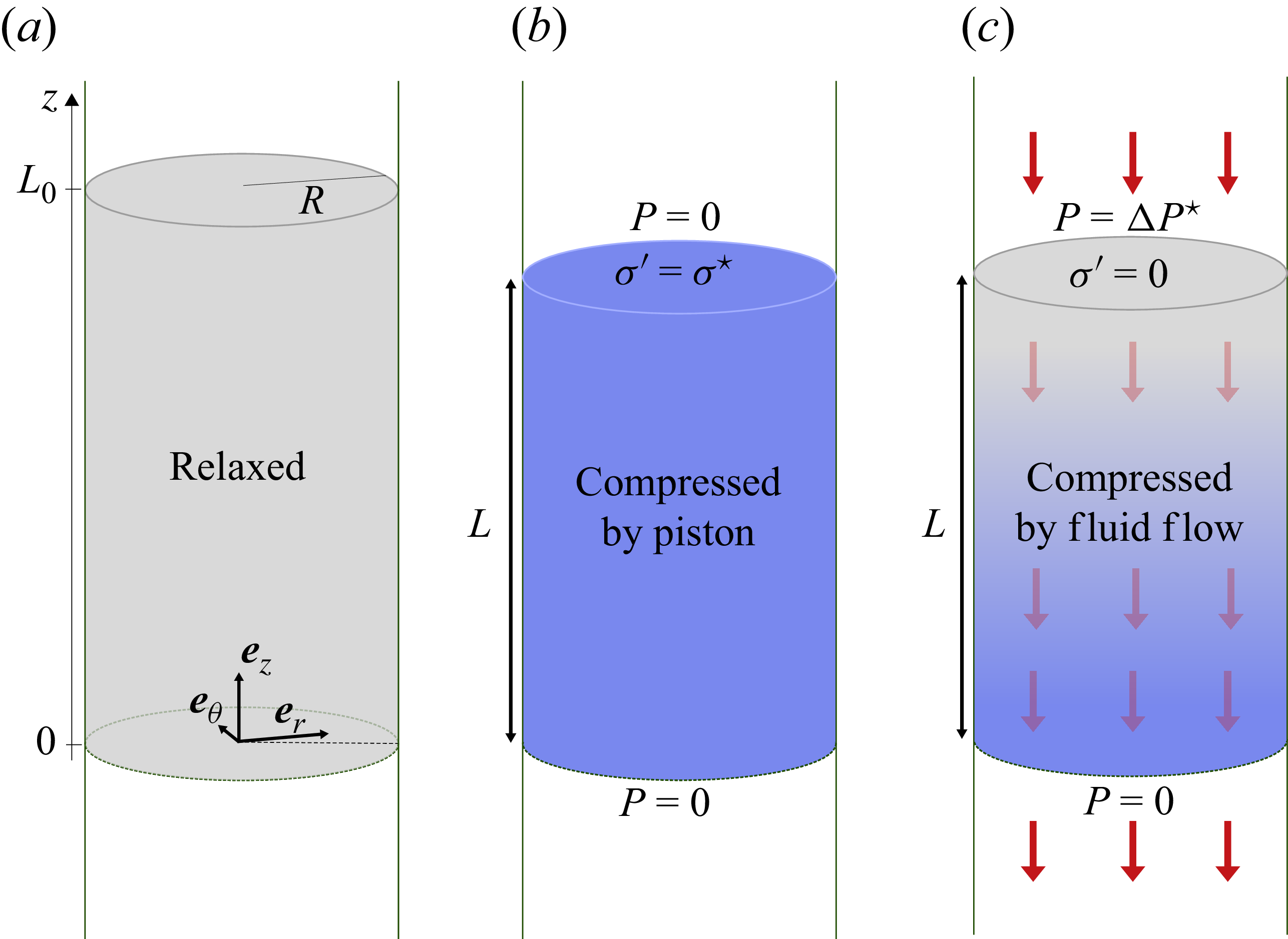
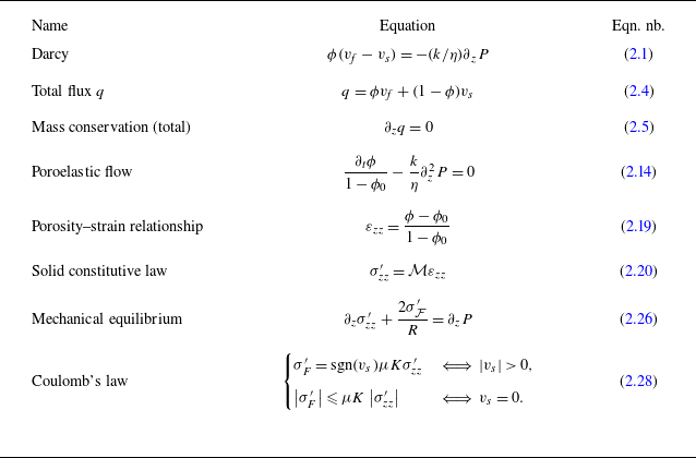


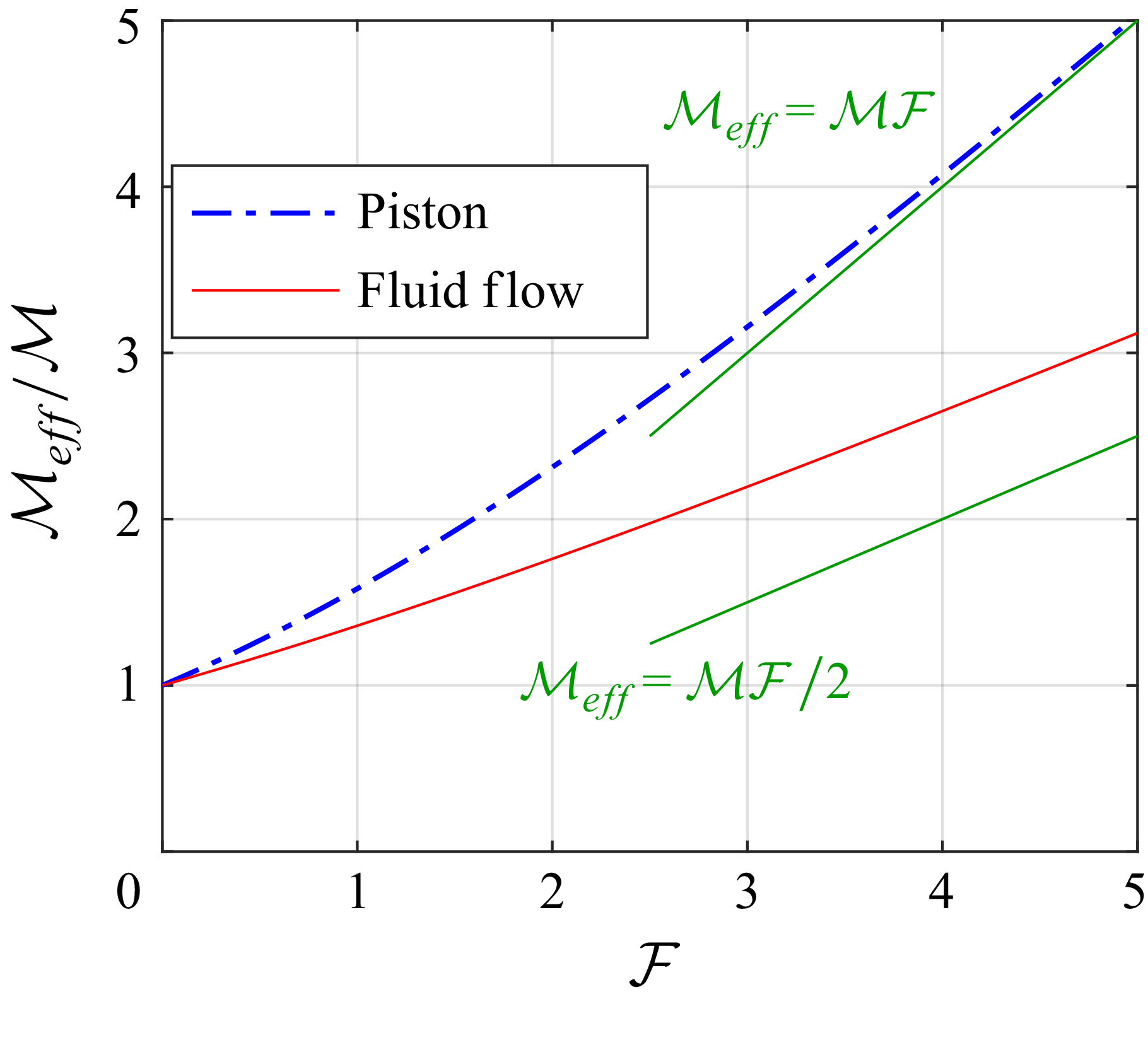


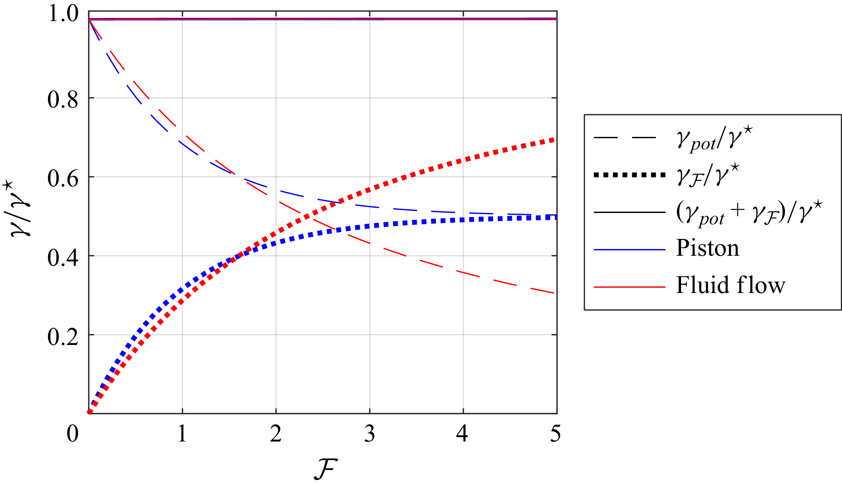

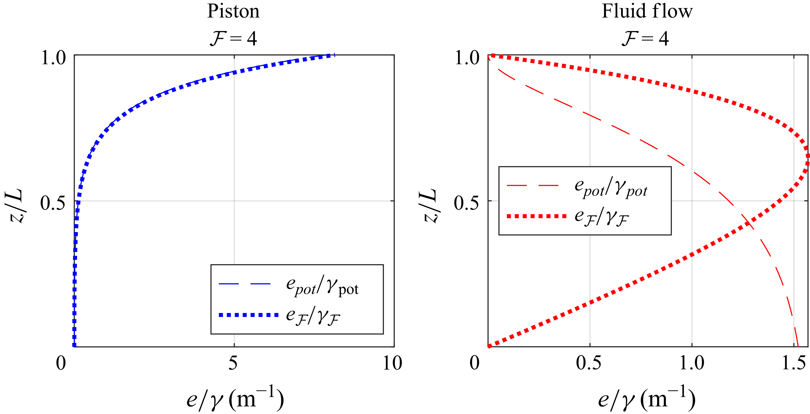
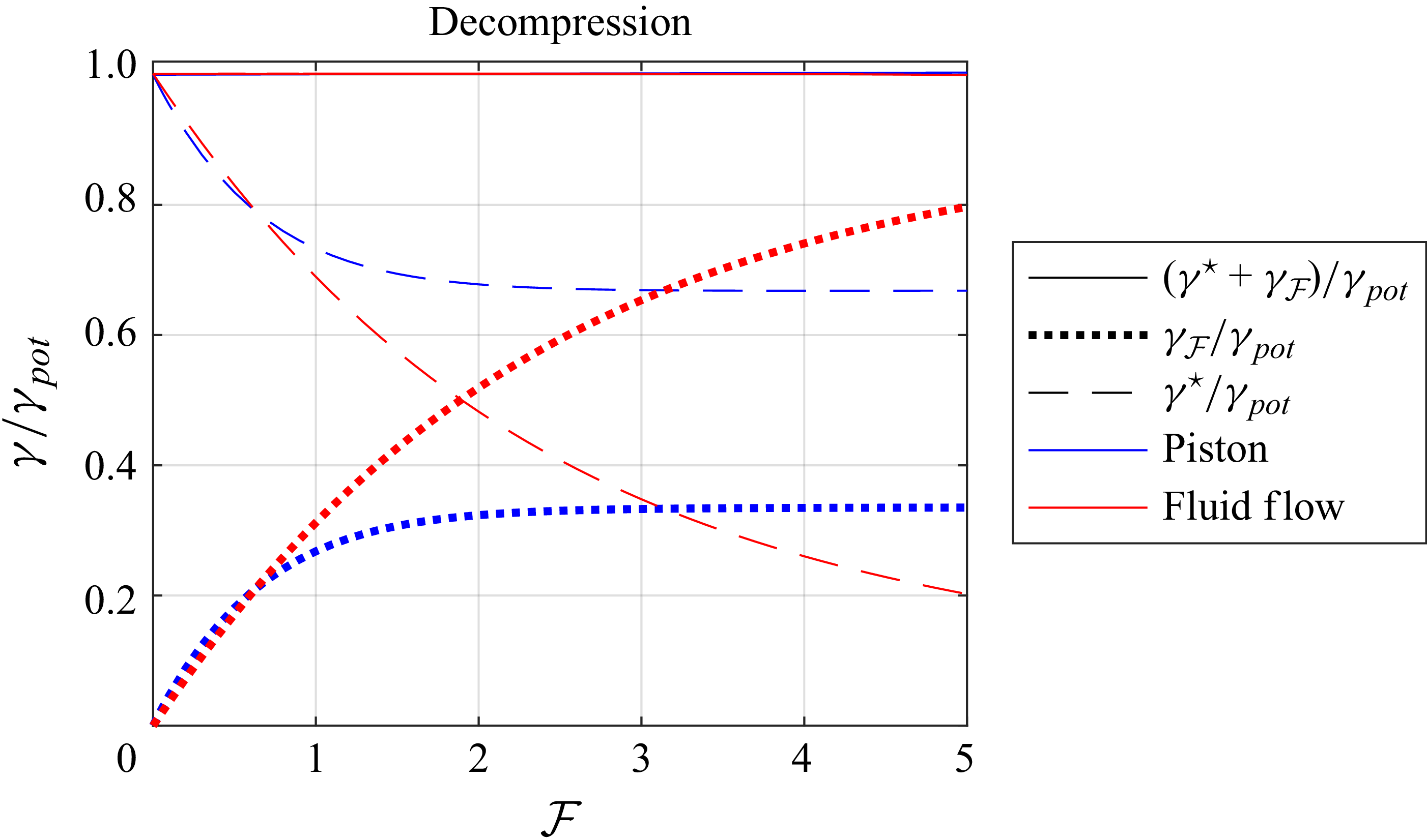


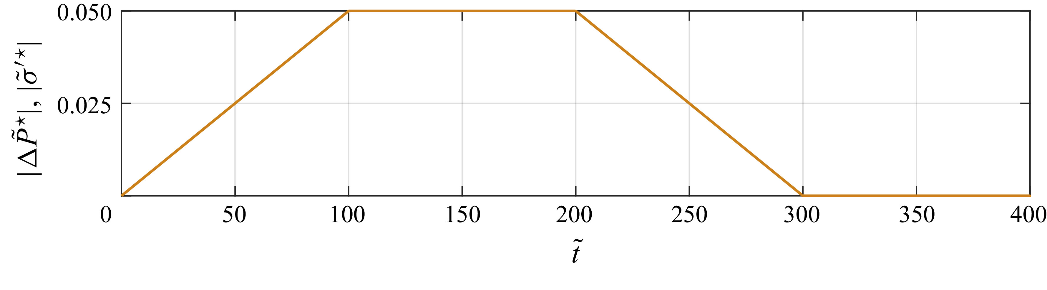

 Open access