


1. Introduction
Mixing refers to the dynamic process by which the scalar gradients are redistributed and homogenised through the combined action of stirring and molecular diffusion (Zhou Reference Zhou2024; Jossy & Gupta Reference Jossy and Gupta2025). Various dynamics can generate kinematics which result in stirring, such as shock-waves driven stirring (Jossy & Gupta Reference Jossy and Gupta2023) and turbulent stirring (Yeung & Sreenivasan Reference Yeung and Sreenivasan2013, Reference Yeung and Sreenivasan2014; Jossy, Awasthi & Gupta Reference Jossy, Awasthi and Gupta2025). The action of stirring by turbulence can be studied in statistically stationary systems with imposed concentration gradients (Yeung & Sreenivasan Reference Yeung and Sreenivasan2014), as well as decaying systems, in which an initially inhomogeneous field of concentration homogenises (Yeung & Sreenivasan Reference Yeung and Sreenivasan2013). In steady mixing setups, the balance between stirring and diffusion signifies mixing. In contrast, unsteady mixing setups are characterised by stirring dominated mixing followed by diffusion dominated smoothening. In this study, we elucidate the effect of temporal correlations on the mixing dynamics of both steady and unsteady mixing set-ups.
Advection of small-scale eddies in a turbulent flow by large, energy-containing eddies is called the random sweeping effect (Tennekes Reference Tennekes1975). Using DNS, Gorbunova et al. (Reference Gorbunova, Balarac, Canet, Eyink and Rossetto2021) showed that the decorrelation time decays as $k^{-1}$
at large wavenumbers, rather than the classical
$k^{-1}$
at large wavenumbers, rather than the classical $k^{-2/3}$
, indicating that the large-scale eddies determine the temporal decorrelation. For homogeneous isotropic turbulence (HIT), Tennekes (Reference Tennekes1975) demonstrated that the Eulerian time spectrum exceeds its Lagrangian counterpart at high frequencies. Building on this idea, Yeung & Sawford (Reference Yeung and Sawford2002) used the random-sweeping framework to elucidate the Lagrangian statistics relevant to mixing and dispersion, and showed that the concept extends to passive scalars. A Lagrangian measure of enhanced stirring is the exponential stretching captured by local finite-time Lyapunov exponents (FTLEs) (Toussaint et al. Reference Toussaint, Carriere, Scott and Gence2000; Aref Reference Aref2020). Götzfried et al. (Reference Götzfried, Emran, Villermaux and Schumacher2019) compared passive-scalar mixing in both Eulerian and Lagrangian descriptions, and showed that the mean mixing time – defined as the duration over which stirring dominates in unsteady mixing setups – is governed by the compressive local FTLE. Additionally, single particle and pair particle dispersion (Sawford Reference Sawford2012) quantify the dynamics of particle displacements and separation in time. At small times, the displacement and separation dynamics are termed to be in the ballistic regime. As the displacements increase, the single particle displacement magnitude transitions to the diffusive regime. The particle pair dispersion transitions to the diffusive regime via the inertial regime where the inertial subrange eddies transport the particles. In this work, we also use these dynamics to quantify the transport of Lagrangian particles by synthetic fields to assess the mixing ability of the fields.
$k^{-2/3}$
, indicating that the large-scale eddies determine the temporal decorrelation. For homogeneous isotropic turbulence (HIT), Tennekes (Reference Tennekes1975) demonstrated that the Eulerian time spectrum exceeds its Lagrangian counterpart at high frequencies. Building on this idea, Yeung & Sawford (Reference Yeung and Sawford2002) used the random-sweeping framework to elucidate the Lagrangian statistics relevant to mixing and dispersion, and showed that the concept extends to passive scalars. A Lagrangian measure of enhanced stirring is the exponential stretching captured by local finite-time Lyapunov exponents (FTLEs) (Toussaint et al. Reference Toussaint, Carriere, Scott and Gence2000; Aref Reference Aref2020). Götzfried et al. (Reference Götzfried, Emran, Villermaux and Schumacher2019) compared passive-scalar mixing in both Eulerian and Lagrangian descriptions, and showed that the mean mixing time – defined as the duration over which stirring dominates in unsteady mixing setups – is governed by the compressive local FTLE. Additionally, single particle and pair particle dispersion (Sawford Reference Sawford2012) quantify the dynamics of particle displacements and separation in time. At small times, the displacement and separation dynamics are termed to be in the ballistic regime. As the displacements increase, the single particle displacement magnitude transitions to the diffusive regime. The particle pair dispersion transitions to the diffusive regime via the inertial regime where the inertial subrange eddies transport the particles. In this work, we also use these dynamics to quantify the transport of Lagrangian particles by synthetic fields to assess the mixing ability of the fields.
In addition to the kinematics of the flow fields, the relative diffusivity of the mixing substance (passive scalars here) to the kinematic viscosity of the fluid, characterised by the inverse of Schmidt number $1/\textit{Sc}$
, governs the spatial distribution features. For
$1/\textit{Sc}$
, governs the spatial distribution features. For $\textit{Sc}=\mathcal{O}(1)$
, the scalar diffusion happens at the same time and length scales as viscous diffusion. Hence, the length scales of the scalar field, which correspond to the inertial subrange of the turbulent field, exhibit similar spatial distribution, resulting in a –5/3 scalar spectrum for sufficiently high Reynolds numbers (Corrsin Reference Corrsin1951; Mydlarski & Warhaft Reference Mydlarski and Warhaft1998; Yeung & Sreenivasan Reference Yeung and Sreenivasan2013). In numerical simulations with limited resources, where very large Reynolds numbers are not generally accessible, the ratio of scalar spectrum to the kinetic energy spectrum will mostly have a flat behaviour. For
$\textit{Sc}=\mathcal{O}(1)$
, the scalar diffusion happens at the same time and length scales as viscous diffusion. Hence, the length scales of the scalar field, which correspond to the inertial subrange of the turbulent field, exhibit similar spatial distribution, resulting in a –5/3 scalar spectrum for sufficiently high Reynolds numbers (Corrsin Reference Corrsin1951; Mydlarski & Warhaft Reference Mydlarski and Warhaft1998; Yeung & Sreenivasan Reference Yeung and Sreenivasan2013). In numerical simulations with limited resources, where very large Reynolds numbers are not generally accessible, the ratio of scalar spectrum to the kinetic energy spectrum will mostly have a flat behaviour. For $\textit{Sc}\gg 1$
, the scalar diffusion is extremely small compared with the kinematic viscosity of the fluid. Hence, the scalar spectrum extends further from the smallest length scales of the fluid motion exhibiting a –1 slope in the spectral space (Batchelor Reference Batchelor1959; Miller & Dimotakis Reference Miller and Dimotakis1996). Yeung & Sreenivasan (Reference Yeung and Sreenivasan2013) showed that for
$\textit{Sc}\gg 1$
, the scalar diffusion is extremely small compared with the kinematic viscosity of the fluid. Hence, the scalar spectrum extends further from the smallest length scales of the fluid motion exhibiting a –1 slope in the spectral space (Batchelor Reference Batchelor1959; Miller & Dimotakis Reference Miller and Dimotakis1996). Yeung & Sreenivasan (Reference Yeung and Sreenivasan2013) showed that for $\textit{Sc}\ll 1$
, the predictions of the so-called BHT theory (Batchelor, Howells & Townsend Reference Batchelor, Howells and Townsend1959) hold and the scalar spectrum exhibits a –17/3 slope in the range where turbulent kinetic energy scales as –5/3 in the spectral space. Derivation of this result relies on the assumption that the turbulent kinetic energy spectrum falls slowly as –5/3 (inertial subrange) and diffusion of the scalar is active in this range (see Batchelor et al. Reference Batchelor, Howells and Townsend1959 for details). It is important to note that the constant kinetic energy spectrum in time in the inertial subrange and the –5/3 variation in spectral space are the only two requirements of this result. The spatio-temporal dynamics, which could help in differentiating a general chaotic fluid motion from turbulence, play no role in this derivation. As we show in this work, a synthetically generated velocity field with a –5/3 range of kinetic energy spectrum, which does not exhibit spatio-temporal correlations as exhibited by turbulence, yields a –17/3 range of scalar spectrum. This highlights that for generally
$\textit{Sc}\ll 1$
, the predictions of the so-called BHT theory (Batchelor, Howells & Townsend Reference Batchelor, Howells and Townsend1959) hold and the scalar spectrum exhibits a –17/3 slope in the range where turbulent kinetic energy scales as –5/3 in the spectral space. Derivation of this result relies on the assumption that the turbulent kinetic energy spectrum falls slowly as –5/3 (inertial subrange) and diffusion of the scalar is active in this range (see Batchelor et al. Reference Batchelor, Howells and Townsend1959 for details). It is important to note that the constant kinetic energy spectrum in time in the inertial subrange and the –5/3 variation in spectral space are the only two requirements of this result. The spatio-temporal dynamics, which could help in differentiating a general chaotic fluid motion from turbulence, play no role in this derivation. As we show in this work, a synthetically generated velocity field with a –5/3 range of kinetic energy spectrum, which does not exhibit spatio-temporal correlations as exhibited by turbulence, yields a –17/3 range of scalar spectrum. This highlights that for generally $\textit{Sc}\lt 1$
scalar mixing, quantification requires more inquiry than the –17/3 variation of the scalar spectrum. For numerical simulations with limited Reynolds number, the ratio of scalar spectrum to the kinetic energy spectrum is expected to show
$\textit{Sc}\lt 1$
scalar mixing, quantification requires more inquiry than the –17/3 variation of the scalar spectrum. For numerical simulations with limited Reynolds number, the ratio of scalar spectrum to the kinetic energy spectrum is expected to show $-4$
scaling in the wavenumber space.
$-4$
scaling in the wavenumber space.
Synthetic turbulent fields aim to reproduce the essential dynamical features of turbulence while avoiding the computational cost associated with solving the full Navier–Stokes equations. Beyond practical utility, such models provide valuable insights into the intrinsic mechanisms of turbulence (Juneja et al. Reference Juneja, Lathrop, Sreenivasan and Stolovitzky1994). Synthetic fields may be generated using a Navier–Stokes implementation while skipping wavenumbers (Sajeev & Donzis Reference Sajeev and Donzis2025) or using stochastic partial differential equations (PDEs; Careta, Sagués & Sancho Reference Careta, Sagués and Sancho1994). The main advantage of working with stochastic PDEs to generate velocity fields that replicate turbulent transport is that building blocks of turbulent motion are revealed. Recently, Jossy et al. (Reference Jossy, Awasthi and Gupta2025) extended Careta et al. (Reference Careta, Sagués and Sancho1994)’s synthetic field framework to three dimensions and showed that such synthetic fields do not replicate the mixing dynamics of Navier–Stokes generated turbulence. In two dimensions, Holzer & Siggia (Reference Holzer and Siggia1994) demonstrated that a stochastically generated two-dimensional (2-D) Gaussian velocity field with a decorrelation time scale $\sim k^{-2/3}$
reproduces the
$\sim k^{-2/3}$
reproduces the $-17/3$
scaling of scalar spectrum when used to mix passive scalars for small
$-17/3$
scaling of scalar spectrum when used to mix passive scalars for small $\textit{Sc}$
and the
$\textit{Sc}$
and the $-1$
scaling in large
$-1$
scaling in large $\textit{Sc}$
cases. While the scalar probability distribution functions (p.d.f.s) were compared to further study the scalar distribution, no direct comparisons with DNS were provided. In this work, we formulate the synthetic generation of homogeneous isotropic turbulent fields capable of replicating the mixing efficiency of turbulent fields. We show that non-Markovian three-dimensional (3-D) homogeneous synthetic velocity fields are closer to turbulence in mixing passive scalars than earlier developed Markovian fields. In the next section, we outline the theoretical basis for constructing non-Markovian synthetic fields and describe the numerical implementation. We then discuss the results in § 3 followed by a summary of findings in § 4.
$\textit{Sc}$
cases. While the scalar probability distribution functions (p.d.f.s) were compared to further study the scalar distribution, no direct comparisons with DNS were provided. In this work, we formulate the synthetic generation of homogeneous isotropic turbulent fields capable of replicating the mixing efficiency of turbulent fields. We show that non-Markovian three-dimensional (3-D) homogeneous synthetic velocity fields are closer to turbulence in mixing passive scalars than earlier developed Markovian fields. In the next section, we outline the theoretical basis for constructing non-Markovian synthetic fields and describe the numerical implementation. We then discuss the results in § 3 followed by a summary of findings in § 4.
2. Theory and numerical simulations
In this section, we outline the details of our DNS and the construction of a synthetic field using the Ornstein–Uhlenbeck equation. We begin by a detailed discussion of the parameters of our homogeneous isotropic DNS in a box and the premise of spatio-temporal correlations in turbulence. Then, we discuss the theoretical development of non-Markovian Gaussian synthetic fields, followed by a discussion of numerical implementation of the synthetic fields, Lagrangian particle tracking simulations and Eulerian passive scalar mixing simulations.
2.1. 3-D DNS of homogeneous isotropic turbulence
The dimensionless form of the incompressible Navier–Stokes equations is given by
 \begin{align} \boldsymbol{\nabla }\boldsymbol{\cdot }\boldsymbol{u} &= 0, \\[-12pt]\nonumber \end{align}
 \begin{align} \frac {\partial \boldsymbol{u}}{\partial t} + (\boldsymbol{u}\boldsymbol{\cdot }\boldsymbol{\nabla })\boldsymbol{u} &= -\boldsymbol{\nabla }\!p + \frac {1}{{\textit{Re}}}\,{\nabla} ^2 \boldsymbol{u} + \boldsymbol{F}, \end{align}
where $\boldsymbol{F}$
represents vortical forcing and
$\boldsymbol{F}$
represents vortical forcing and ${\textit{Re}}$
is the characteristic Reynolds number given as
${\textit{Re}}$
is the characteristic Reynolds number given as ${\textit{Re}} =U_0 L_0/\nu _0$
. The quantities with the subscript
${\textit{Re}} =U_0 L_0/\nu _0$
. The quantities with the subscript $()_0$
are the reference scales used for non-dimensionalisation. The pressure
$()_0$
are the reference scales used for non-dimensionalisation. The pressure $p$
is obtained from the velocity field using the pressure Poisson equation. We use a message passing interface (MPI) parallelised Fourier pseudo-spectral solver using the P3DFFT library (Pekurovsky Reference Pekurovsky2012) to carry out the DNS and obtain the statistically stationary homogeneous isotropic turbulent fields. Time integration is performed using a fourth-order Runge–Kutta scheme. Aliasing errors are eliminated using the
$p$
is obtained from the velocity field using the pressure Poisson equation. We use a message passing interface (MPI) parallelised Fourier pseudo-spectral solver using the P3DFFT library (Pekurovsky Reference Pekurovsky2012) to carry out the DNS and obtain the statistically stationary homogeneous isotropic turbulent fields. Time integration is performed using a fourth-order Runge–Kutta scheme. Aliasing errors are eliminated using the $2/3$
de-aliasing rule, such that the maximum resolvable wavenumber is
$2/3$
de-aliasing rule, such that the maximum resolvable wavenumber is $k_{\textit{max}} = N/3$
, where
$k_{\textit{max}} = N/3$
, where $N$
is the number of Fourier modes in each direction. The computational domain is a triply periodic cube of side
$N$
is the number of Fourier modes in each direction. The computational domain is a triply periodic cube of side $2\pi$
. We follow Eswaran & Pope (Reference Eswaran and Pope1988), and use the Ornstein–Uhlenbeck process to force and maintain a statistically stationary homogeneous isotropic turbulent field. We refer the reader to Jossy et al. (Reference Jossy, Awasthi and Gupta2025) for the details of the forcing method. We control the energy injection rate (
$2\pi$
. We follow Eswaran & Pope (Reference Eswaran and Pope1988), and use the Ornstein–Uhlenbeck process to force and maintain a statistically stationary homogeneous isotropic turbulent field. We refer the reader to Jossy et al. (Reference Jossy, Awasthi and Gupta2025) for the details of the forcing method. We control the energy injection rate ( $\sigma$
) and restrict the energy injection to only the large scales (
$\sigma$
) and restrict the energy injection to only the large scales ( $k_{\!f}$
) such that the small scales are not directly affected by the forcing. To obtain statistically stationary turbulence, the simulations are run until the mean rate of energy injection equals the mean dissipation rate,
$k_{\!f}$
) such that the small scales are not directly affected by the forcing. To obtain statistically stationary turbulence, the simulations are run until the mean rate of energy injection equals the mean dissipation rate, $ \ \overline {\varepsilon }$
, where
$ \ \overline {\varepsilon }$
, where $\overline {()}$
denotes the time average. We consider two turbulent fields with differing turbulence intensities, characterised by their Taylor Reynolds numbers, i.e.
$\overline {()}$
denotes the time average. We consider two turbulent fields with differing turbulence intensities, characterised by their Taylor Reynolds numbers, i.e. $\textit{Re}_\lambda = 53$
and
$\textit{Re}_\lambda = 53$
and $115$
. To ensure adequate numerical resolution, we ensure that the Kolmogorov length scale (
$115$
. To ensure adequate numerical resolution, we ensure that the Kolmogorov length scale ( $\eta = {\textit{Re}}^{-3/4} \overline {\varepsilon }^{1/4}$
) is resolved by the maximum resolvable wavenumber of the simulation,
$\eta = {\textit{Re}}^{-3/4} \overline {\varepsilon }^{1/4}$
) is resolved by the maximum resolvable wavenumber of the simulation, $k_{\textit{max}}$
, and we therefore follow the criterion
$k_{\textit{max}}$
, and we therefore follow the criterion $k_{\textit{max}}\eta \approx 1.5$
. The forcing parameters, resolution details and the indicators for the two simulations are summarised in table 1. The integral length scale
$k_{\textit{max}}\eta \approx 1.5$
. The forcing parameters, resolution details and the indicators for the two simulations are summarised in table 1. The integral length scale $L$
is calculated as (Meldi & Sagaut Reference Meldi and Sagaut2017)
$L$
is calculated as (Meldi & Sagaut Reference Meldi and Sagaut2017)
 \begin{equation} L = \frac {3\pi }{4}\frac {\sum {E(k)}/{k}}{\sum E(k)}, \end{equation}
where $E(k)$
is the binned energy spectra (hereafter, just referred as energy spectra) averaged over spherical shells and summation is over the bins.
$E(k)$
is the binned energy spectra (hereafter, just referred as energy spectra) averaged over spherical shells and summation is over the bins.
Simulation parameters for DNS of forced homogeneous isotropic turbulence.

For fully developed homogeneous isotropic turbulence, the kinetic energy spectra $E(k)$
in the inertial range is given by
$E(k)$
in the inertial range is given by
 \begin{equation} E(k) = C_{\!K} \overline { \varepsilon }^{2/3} k^{-5/3}, \end{equation}
where $C_{\!K}$
is the Kolmogorov constant (Yeung & Zhou Reference Yeung and Zhou1997). Figure 1
$C_{\!K}$
is the Kolmogorov constant (Yeung & Zhou Reference Yeung and Zhou1997). Figure 1 $(a)$
shows the compensated spherically averaged kinetic energy spectra for both the simulations. We see that the inertial range follows a scaling of
$(a)$
shows the compensated spherically averaged kinetic energy spectra for both the simulations. We see that the inertial range follows a scaling of $-5/3$
with the higher Taylor Reynolds number exhibiting a wider range of inertial scales spanning approximately two decades. The horizontal line in figure 1
$-5/3$
with the higher Taylor Reynolds number exhibiting a wider range of inertial scales spanning approximately two decades. The horizontal line in figure 1 $(a)$
shows that the universal constant is
$(a)$
shows that the universal constant is $C_{\!K}=1.8$
, which is in accordance with the value reported by Ishihara et al. (Reference Ishihara, Morishita, Yokokawa, Uno and Kaneda2016). The digitised compensated energy spectra from Gorbunova et al. (Reference Gorbunova, Balarac, Canet, Eyink and Rossetto2021) are also shown in figure 1 for comparison. The de-correlation time associated with the scale at wavenumber
$C_{\!K}=1.8$
, which is in accordance with the value reported by Ishihara et al. (Reference Ishihara, Morishita, Yokokawa, Uno and Kaneda2016). The digitised compensated energy spectra from Gorbunova et al. (Reference Gorbunova, Balarac, Canet, Eyink and Rossetto2021) are also shown in figure 1 for comparison. The de-correlation time associated with the scale at wavenumber $k$
is given by
$k$
is given by
 \begin{equation} \tau _c(k) = \int \limits _0^\infty \frac {\langle \hat {\boldsymbol{u}}(\boldsymbol{k},t)\boldsymbol{\cdot }\hat {\boldsymbol{u}^*} (\boldsymbol{k},t+s)\rangle }{\langle |\hat {\boldsymbol{u}}(\boldsymbol{k},t)|^2 \rangle }\, {\rm d}s, \end{equation}
where $\hat {u}(\boldsymbol{k},t)$
denotes the Fourier transformed velocity field,
$\hat {u}(\boldsymbol{k},t)$
denotes the Fourier transformed velocity field, $s$
is the time lag and
$s$
is the time lag and $\langle \rangle$
denotes ensemble average over modes with the same wavenumber magnitude
$\langle \rangle$
denotes ensemble average over modes with the same wavenumber magnitude $k$
. The time-averaged mean turbulent kinetic energies
$k$
. The time-averaged mean turbulent kinetic energies $\overline {\langle {\textit{TKE}} \rangle _x}$
and the time averaged root-mean-square (r.m.s.) velocity
$\overline {\langle {\textit{TKE}} \rangle _x}$
and the time averaged root-mean-square (r.m.s.) velocity $\overline {u'}=\sqrt {2{\overline {\langle {\textit{TKE}} \rangle _x}}/3}$
(where
$\overline {u'}=\sqrt {2{\overline {\langle {\textit{TKE}} \rangle _x}}/3}$
(where $\langle \rangle _x$
denotes spatial average) for both cases are listed in table 1. These values are used in the generation of the synthetic fields, where we require the synthetic velocity fields to have identical energy input.
$\langle \rangle _x$
denotes spatial average) for both cases are listed in table 1. These values are used in the generation of the synthetic fields, where we require the synthetic velocity fields to have identical energy input.
(a) Compensated kinetic energy spectrum for different ${\textit{Re}}_\lambda$
versus wavenumber normalised by the integral length scale.
${\textit{Re}}_\lambda$
versus wavenumber normalised by the integral length scale. $\overline {\varepsilon }$
is the time averaged dissipation rate,
$\overline {\varepsilon }$
is the time averaged dissipation rate, $L$
is the integral length scale. (b) De-correlation time
$L$
is the integral length scale. (b) De-correlation time $\tau _c$
dependence on wavenumber in log–log space with an arbitrary black dashed line of slope -1.
$\tau _c$
dependence on wavenumber in log–log space with an arbitrary black dashed line of slope -1.

Figure 1 $(b)$
shows the dependence of the de-correlation time scale
$(b)$
shows the dependence of the de-correlation time scale $\tau _c$
with wavenumber for the two simulations. For both simulations, we see that
$\tau _c$
with wavenumber for the two simulations. For both simulations, we see that $\tau _c \sim k^{-1}$
over most scales, with deviations only at small
$\tau _c \sim k^{-1}$
over most scales, with deviations only at small $k$
, indicating Reynolds-number independence. The results obtained from the simulations are in agreement with those reported by Gorbunova et al. (Reference Gorbunova, Balarac, Canet, Eyink and Rossetto2021) for the JHTDB, which is also generated using random forcing at large scales. This scaling is a result of the random sweeping effect, where the velocity scale of large length scales advects the velocity perturbations at smaller length scale (Yeung & Sawford Reference Yeung and Sawford2002).
$k$
, indicating Reynolds-number independence. The results obtained from the simulations are in agreement with those reported by Gorbunova et al. (Reference Gorbunova, Balarac, Canet, Eyink and Rossetto2021) for the JHTDB, which is also generated using random forcing at large scales. This scaling is a result of the random sweeping effect, where the velocity scale of large length scales advects the velocity perturbations at smaller length scale (Yeung & Sawford Reference Yeung and Sawford2002).
2.2. 3-D time correlated non-Markovian synthetic field
Careta et al. (Reference Careta, Sagués and Sancho1994) proposed a 2-D homogeneous isotropic velocity field using the Ornstein–Uhlenbeck process. Jossy et al. (Reference Jossy, Awasthi and Gupta2025) extended the methodology to generate 3-D homogeneous isotropic velocity field. In this work, we extend the 3-D synthetic velocity field proposed by Jossy et al. (Reference Jossy, Awasthi and Gupta2025) to generate a 3-D non-Markovian homogeneous isotropic velocity field. We assume all fields in the spatial domain are real and vanish outside the box of size $(2\pi )^3$
. We define a vector potential
$(2\pi )^3$
. We define a vector potential $\hat {\boldsymbol{{\eta }}}(\boldsymbol{k},t)$
in the spectral space which is an Ornstein–Uhlenbeck process with different decaying time scales given as
$\hat {\boldsymbol{{\eta }}}(\boldsymbol{k},t)$
in the spectral space which is an Ornstein–Uhlenbeck process with different decaying time scales given as
 \begin{equation} \frac {{\rm d}\hat {\boldsymbol{\eta }}(\boldsymbol{k},t)}{{\rm d}t} = - \frac {\hat {\boldsymbol{\eta }}(\boldsymbol{k},t)}{\tau (\boldsymbol{k})} + \frac {\hat {Q}(\boldsymbol{k})}{\tau (\boldsymbol{k})}\hat {\boldsymbol{\chi }}(\boldsymbol{k},t), \end{equation}
where $\tau (\boldsymbol{k})$
is the spectrally varying relaxation time scale,
$\tau (\boldsymbol{k})$
is the spectrally varying relaxation time scale, $\hat {Q}(\boldsymbol{k})$
is the filtering kernel used to achieve a desired energy spectrum and
$\hat {Q}(\boldsymbol{k})$
is the filtering kernel used to achieve a desired energy spectrum and $\hat {\boldsymbol{\chi }}(\boldsymbol{k},t)$
is the Fourier transform of
$\hat {\boldsymbol{\chi }}(\boldsymbol{k},t)$
is the Fourier transform of $\boldsymbol{\chi }(\boldsymbol{r},t)$
, which is a delta correlated white noise vector with zero mean and its correlation tensor is defined as
$\boldsymbol{\chi }(\boldsymbol{r},t)$
, which is a delta correlated white noise vector with zero mean and its correlation tensor is defined as
 \begin{equation} \langle \chi _i(\boldsymbol{x},t) \chi _{\!j}(\boldsymbol{x}+\boldsymbol{r},t+s) \rangle = 2\epsilon \delta _{\textit{ij}} \delta (\boldsymbol{r})\delta (s), \end{equation}
where $\epsilon$
is the intensity of the white noise,
$\epsilon$
is the intensity of the white noise, $\delta _{\textit{ij}}$
is the Kronecker delta, and
$\delta _{\textit{ij}}$
is the Kronecker delta, and $\delta (\boldsymbol{r})$
and
$\delta (\boldsymbol{r})$
and $\delta (s)$
are 3-D and one-dimensional Dirac delta functions, respectively. The solution of the vector potential in the Fourier space is given as
$\delta (s)$
are 3-D and one-dimensional Dirac delta functions, respectively. The solution of the vector potential in the Fourier space is given as
 \begin{equation} \hat {\boldsymbol{\eta }}(\boldsymbol{k},t) = \hat {\boldsymbol{\eta }}(\boldsymbol{k},0)e^{-\frac {t}{\tau (\boldsymbol{k})}} + \int \limits _0^t \frac {{\hat {Q}}(\boldsymbol{k})}{\tau (\boldsymbol{k})}\hat {\boldsymbol{\chi }}(\boldsymbol{k},t') e^{\frac {t'-t}{\tau (\boldsymbol{k})}}\, {\rm d}t', \end{equation}
with the time correlation tensor defined as
 \begin{align} \langle \hat {\eta }^*_p(\boldsymbol{k},t)\hat {\eta }_q(\boldsymbol{k},t+s) \rangle &= |\hat {Q}|^2 \frac {2\epsilon \delta _{pq} e^{-s/\tau (\boldsymbol{k})}}{(2\pi )^3 \tau (\boldsymbol{k})^2} \int \limits _0^t \int \limits _0^{t+s} \delta (t'-t'') e^{\frac {t'+t'' - 2t}{\tau (\boldsymbol{k})}} \, {\rm d}t' \, {\rm d}t''. \end{align}
When, $t\to \infty$
, (2.8) yields
$t\to \infty$
, (2.8) yields
 \begin{equation} \lim _{t\to \infty }\langle {\hat {\eta }^*_p(\boldsymbol{k},t)\hat {\eta }_q(\boldsymbol{k},t+s)}\rangle = \frac {\epsilon \delta _{pq}|\hat {Q}|^2}{(2\pi )^3\tau (\boldsymbol{k})}e^{-s/\tau (\boldsymbol{k})} = \hat {C}^\eta (\boldsymbol{k}, s)\delta _{pq}. \end{equation}
To estimate the velocity auto-correlation time scale (decorrelation time for a particular scale) for synthetic fields, we substitute (2.9) in
 \begin{equation} \phi _{ii}(\boldsymbol{k},s) = \left \langle \hat {\boldsymbol{u}}^*(\boldsymbol{k},t)\boldsymbol{\cdot }\hat {\boldsymbol{u}}(\boldsymbol{k},t+s)\right \rangle = k^2\big \langle \hat {\eta }^*_p\hat {\eta }_p\big \rangle - k_mk_l\left \langle \hat {\eta }^*_m\hat {\eta }_l\right \rangle \!, \end{equation}
to obtain
 \begin{equation} \tau _c(\boldsymbol{k}) = \frac {\int ^\infty _0 \phi _{ii}(\boldsymbol{k},s)\,{\rm d}s}{\phi _{ii}(\boldsymbol{k},0)} = \tau (\boldsymbol{k}). \end{equation}
Equation (2.11) confirms that the decorrelation time scale of the velocity field at length scale $1/|\boldsymbol{k}|$
is
$1/|\boldsymbol{k}|$
is $\tau (\boldsymbol{k})$
, which may be averaged over modes with same wavenumber magnitude. The auto-correlation of the Fourier transform of velocity
$\tau (\boldsymbol{k})$
, which may be averaged over modes with same wavenumber magnitude. The auto-correlation of the Fourier transform of velocity $\phi _{ii}(\boldsymbol{k},s)$
is related to the energy spectra
$\phi _{ii}(\boldsymbol{k},s)$
is related to the energy spectra $E(k)$
as (Batchelor Reference Batchelor1953)
$E(k)$
as (Batchelor Reference Batchelor1953)
 \begin{equation} E(k) = 2\pi k^2 \phi _{ii} = \frac {k^4 \epsilon |\hat {Q}|^2}{2\pi ^2\tau }, \end{equation}
where $k=|\boldsymbol{k}|$
. A desired spectral variation in the kinetic energy is obtained using the filtering kernel
$k=|\boldsymbol{k}|$
. A desired spectral variation in the kinetic energy is obtained using the filtering kernel $\hat {Q}(\boldsymbol{k})$
defined as
$\hat {Q}(\boldsymbol{k})$
defined as
 \begin{equation} \hat {Q}_I(\boldsymbol{k}) = (1+\ell ^2 k^2)^{-n}, \end{equation}
where $\ell$
denotes a length scale and
$\ell$
denotes a length scale and $n$
is a parameter that governs the sharpness of the filter in spectral space. The subscript
$n$
is a parameter that governs the sharpness of the filter in spectral space. The subscript $()_I$
denotes that this form of
$()_I$
denotes that this form of $\hat {Q}$
is used for achieving the so-called ideal spectra in our synthetic fields, i.e.
$\hat {Q}$
is used for achieving the so-called ideal spectra in our synthetic fields, i.e. $E(k)\sim k^{-5/3}$
for
$E(k)\sim k^{-5/3}$
for $\ell k \gg 1$
by varying
$\ell k \gg 1$
by varying $n$
. In this work, we use
$n$
. In this work, we use $\ell =1$
. For spectrally varying
$\ell =1$
. For spectrally varying $\tau (\boldsymbol{k})$
, the process
$\tau (\boldsymbol{k})$
, the process $\boldsymbol{\eta }(\boldsymbol{x},t)$
is non-Markovian. In the spatial domain, the time correlation is given by
$\boldsymbol{\eta }(\boldsymbol{x},t)$
is non-Markovian. In the spatial domain, the time correlation is given by
 \begin{equation} \left \langle \eta _p(\boldsymbol{x},t)\eta _q(\boldsymbol{x}+\boldsymbol{r},t+s)\right \rangle = \int \limits _{\mathbb{R}^3}\big \langle \hat {\eta }^*_p(\boldsymbol{k},t)\hat {\eta }_q(\boldsymbol{k},t+s)\big \rangle e^{i\boldsymbol{k}\boldsymbol{\cdot }\boldsymbol{r}}\,{\rm d}\boldsymbol{k}, \end{equation}
which yields for $\hat {Q}_I(\boldsymbol{k})$
from (2.13),
$\hat {Q}_I(\boldsymbol{k})$
from (2.13),
 \begin{equation} C^\eta _{pq}(\boldsymbol{r}, s) = \left \langle \eta _p(\boldsymbol{x},t)\eta _q(\boldsymbol{x}+\boldsymbol{r},t+s)\right \rangle = {\epsilon \delta _{pq}}\int \limits _{\mathbb{R}^3}\frac {(1+\ell ^2 k^2)^{-2n}}{\tau (\boldsymbol{k})}e^{-s/\tau (\boldsymbol{k})}e^{i\boldsymbol{k}\boldsymbol{\cdot }\boldsymbol{r}}\,{\rm d}\boldsymbol{k}, \end{equation}
which resembles the correlation field studied by Chaves et al. (Reference Chaves, Gawedzki, Horvai, Kupiainen and Vergassola2003) and studied recently by Chatelain et al. (Reference Chatelain, Domingues Lemos, Ruffenach, Bourgoin, Bréhier, Chevillard, Sibgatullin and Volk2026). Using (2.10), we obtain
 \begin{equation} \big \langle \hat {u}^*_p(\boldsymbol{k},t)\hat {u}_q(\boldsymbol{k}, t+s) \big \rangle = \hat {C}^{\eta }(\boldsymbol{k},s)\big (\delta _{pq}k^2 - k_pk_q\big ), \end{equation}
and we can compute correlation tensors of $\boldsymbol{A}\kern-0.5pt\boldsymbol{A}$
and
$\boldsymbol{A}\kern-0.5pt\boldsymbol{A}$
and $\boldsymbol{A}\kern-0.5pt\boldsymbol{A}^T$
, where
$\boldsymbol{A}\kern-0.5pt\boldsymbol{A}^T$
, where $\boldsymbol{A} = \boldsymbol{\nabla }\boldsymbol{u}$
. In the spectral domain,
$\boldsymbol{A} = \boldsymbol{\nabla }\boldsymbol{u}$
. In the spectral domain,
 \begin{equation} \big \langle \hat {\boldsymbol{A}}^*\hat {\boldsymbol{A}} \big \rangle = \big \langle \hat {A}^*_{lm}\hat {A}_{mn} \big \rangle = k_lk_m\left \langle \hat {u}^*_m\hat {u}_n \right \rangle = 0 \end{equation}
and
 \begin{equation} \big \langle \hat {\boldsymbol{A}}^*\hat {\boldsymbol{A}}^T \big \rangle = \big \langle \hat {A}^*_{lm}\hat {A}_{nm} \big \rangle = k_lk_n\left \langle \hat {u}^*_m\hat {u}_m \right \rangle = 2k^2\hat {C}^{\eta }(\boldsymbol{k},s)k_lk_n.\, \end{equation}
We will use $\hat {\boldsymbol{C}}^A(\boldsymbol{k}, s) = \langle \hat {\boldsymbol{A}}^*\hat {\boldsymbol{A}}^T \rangle$
(see § 2.3). In the spatial domain, the correlation tensor
$\hat {\boldsymbol{C}}^A(\boldsymbol{k}, s) = \langle \hat {\boldsymbol{A}}^*\hat {\boldsymbol{A}}^T \rangle$
(see § 2.3). In the spatial domain, the correlation tensor $\boldsymbol{C}^A(\boldsymbol{r}, s) = \boldsymbol{A}\kern-0.5pt\boldsymbol{A}^T$
is given by
$\boldsymbol{C}^A(\boldsymbol{r}, s) = \boldsymbol{A}\kern-0.5pt\boldsymbol{A}^T$
is given by
 \begin{equation} C^A_{nl}(\boldsymbol{r},s) = 2\int \limits _{\mathbb{R}^3}k^2\hat {C}^{\eta }(\boldsymbol{k},s)k_nk_l e^{i\boldsymbol{k}\boldsymbol{\cdot }\boldsymbol{r}}\,{\rm d}\boldsymbol{k}.\, \end{equation}
In § 2.3, we use $\boldsymbol{C}^A$
to simplify the average strain tensor of deformation to compute the small time deformation characteristics in random unsteady fields.
$\boldsymbol{C}^A$
to simplify the average strain tensor of deformation to compute the small time deformation characteristics in random unsteady fields.
Equation (2.15) highlights that for spectrally varying $\tau (\boldsymbol{k})$
, at a spatial point,
$\tau (\boldsymbol{k})$
, at a spatial point, $\boldsymbol{\eta }$
is a non-Markovian field since the integral cannot be simplified to an exponentially decaying time correlation, unless
$\boldsymbol{\eta }$
is a non-Markovian field since the integral cannot be simplified to an exponentially decaying time correlation, unless $\tau (\boldsymbol{k})=\mathrm{constant}$
with respect to
$\tau (\boldsymbol{k})=\mathrm{constant}$
with respect to $\boldsymbol{k}$
(the Markovian case). As we show in § 3, the velocity field generated due to Markovian
$\boldsymbol{k}$
(the Markovian case). As we show in § 3, the velocity field generated due to Markovian $\boldsymbol{\eta }$
leads to weak scalar mixing, while the non-Markovian velocity field exhibits mixing dynamics very similar to turbulence. As shown in (2.11),
$\boldsymbol{\eta }$
leads to weak scalar mixing, while the non-Markovian velocity field exhibits mixing dynamics very similar to turbulence. As shown in (2.11), $\tau (\boldsymbol{k})$
is the time after which velocity at length scale
$\tau (\boldsymbol{k})$
is the time after which velocity at length scale $\sim 1/|\boldsymbol{k}|$
gets de-correlated with its history. In the context of hydrodynamic turbulence,
$\sim 1/|\boldsymbol{k}|$
gets de-correlated with its history. In the context of hydrodynamic turbulence, $\tau (\boldsymbol{k})$
can be compared with the residence time of velocity perturbations at a particular length scale, before they get completely renewed. While the time scale for eddies at wavenumber
$\tau (\boldsymbol{k})$
can be compared with the residence time of velocity perturbations at a particular length scale, before they get completely renewed. While the time scale for eddies at wavenumber $k$
can be shown to be
$k$
can be shown to be ${\sim} k^{-({2}/{3})}$
(Pope Reference Pope2001), the so-called random sweeping effect (Yeung & Sawford Reference Yeung and Sawford2002; Wilczek & Narita Reference Wilczek and Narita2012; Gorbunova et al. Reference Gorbunova, Balarac, Canet, Eyink and Rossetto2021) results in
${\sim} k^{-({2}/{3})}$
(Pope Reference Pope2001), the so-called random sweeping effect (Yeung & Sawford Reference Yeung and Sawford2002; Wilczek & Narita Reference Wilczek and Narita2012; Gorbunova et al. Reference Gorbunova, Balarac, Canet, Eyink and Rossetto2021) results in $\tau \sim (u_0 k )^{-1}$
, where
$\tau \sim (u_0 k )^{-1}$
, where $u_0$
is the large eddy velocity scale. Using a radial function for
$u_0$
is the large eddy velocity scale. Using a radial function for $\tau (\boldsymbol{k}) = 1/k$
and substituting
$\tau (\boldsymbol{k}) = 1/k$
and substituting $n=5/3$
in (2.13), we obtain the integral in time correlations of
$n=5/3$
in (2.13), we obtain the integral in time correlations of $\boldsymbol{\eta }, \boldsymbol{u}$
and
$\boldsymbol{\eta }, \boldsymbol{u}$
and $\boldsymbol{\nabla }\boldsymbol{u}$
as
$\boldsymbol{\nabla }\boldsymbol{u}$
as
 \begin{equation} I_{\textit{NM}}(s) = \int \limits ^\infty _0k^{\beta +3}\big (1 + \ell ^2k^2\big )^{-10/3}e^{-ks}\,{\rm d}k, \end{equation}
where $\beta = 0, 2, 4$
for
$\beta = 0, 2, 4$
for $\boldsymbol{\eta }, \boldsymbol{u}$
(cf. (2.16)) and
$\boldsymbol{\eta }, \boldsymbol{u}$
(cf. (2.16)) and $\boldsymbol{\nabla }\boldsymbol{u}$
(cf. (2.18)), respectively. For small times
$\boldsymbol{\nabla }\boldsymbol{u}$
(cf. (2.18)), respectively. For small times $ks\ll 1$
, the integral can be approximated as
$ks\ll 1$
, the integral can be approximated as
 \begin{equation} I_{\textit{NM}}\approx \int \limits ^\infty _0 \frac {k^{\beta +3}}{(1+\ell ^2k^2)^{10/3}}\left (1 - ks + \frac {k^2s^2}{2} + {\cdots} \right )\,{\rm d}k. \end{equation}
For $\beta =0, 2, 4$
, the first term in the previous expansion can be evaluated exactly along with the odd powers of
$\beta =0, 2, 4$
, the first term in the previous expansion can be evaluated exactly along with the odd powers of $k$
in the numerator. Even powers of
$k$
in the numerator. Even powers of $k$
in the numerator need to be computed numerically. To obtain approximate long time behaviour, we separate the limits of integration based on different scales. For
$k$
in the numerator need to be computed numerically. To obtain approximate long time behaviour, we separate the limits of integration based on different scales. For $\ell K_0 \ll 1$
, we can expand the filter function
$\ell K_0 \ll 1$
, we can expand the filter function $Q$
using the binomial. For large
$Q$
using the binomial. For large $k$
, the filter function decays rapidly. Ignoring the large
$k$
, the filter function decays rapidly. Ignoring the large $k$
contributions, we obtain
$k$
contributions, we obtain
 \begin{align} I_{\textit{NM}} &\approx \int \limits ^{K_0}_0 k^{\beta + 3}\left (1-\frac {10}{3}\ell ^2k^2 + \frac {65}{9}\ell ^4k^4+{\cdots} \right )e^{-ks}\,{\rm d}k \nonumber \\ &= \left (\int \limits ^{K_0}_0k^{\beta +3}e^{-ks}\,{\rm d}k - \frac {10}{3}\ell ^2\int \limits ^{K_0}_0k^{\beta +5}e^{-ks}\,{\rm d}k + {\cdots} \right )\! .\end{align}
The leading order term highlights that the large scales make the non-Markovian contribution to the correlations,
 \begin{equation} I_{\textit{NM}}\sim \frac {1}{s^{4+\beta }}. \end{equation}
Figure 2 shows the variation of $I_{\textit{NM}}$
with
$I_{\textit{NM}}$
with $s$
obtained using numerical integration of (2.20) for
$s$
obtained using numerical integration of (2.20) for $\beta =0$
and
$\beta =0$
and $\beta =2$
. For small times, the behaviour is identical to a Markovian field which is depicted by the straight line in the semi-log plot. For large times, the time correlation clearly decays as in (2.23) (
$\beta =2$
. For small times, the behaviour is identical to a Markovian field which is depicted by the straight line in the semi-log plot. For large times, the time correlation clearly decays as in (2.23) ( $ s^{-4}$
for
$ s^{-4}$
for $\beta =0$
and
$\beta =0$
and $ s^{-6}$
for
$ s^{-6}$
for $\beta =2$
), slower than
$\beta =2$
), slower than $e^{-s}$
, thus confirming the non-Markovian nature of the
$e^{-s}$
, thus confirming the non-Markovian nature of the $\boldsymbol{\eta }(\boldsymbol{x}, t)$
field and, consequently, that of
$\boldsymbol{\eta }(\boldsymbol{x}, t)$
field and, consequently, that of $\boldsymbol{u}(\boldsymbol{x}, t)$
and
$\boldsymbol{u}(\boldsymbol{x}, t)$
and $\boldsymbol{\nabla }\boldsymbol{u}(\boldsymbol{x}, t)$
. It is important to note that for each Fourier mode, the evolution is Markovian, yet the spatio-temporal correlations show that in physical space, the fields are essentially non-Markovian. Furthermore, the long time variation of
$\boldsymbol{\nabla }\boldsymbol{u}(\boldsymbol{x}, t)$
. It is important to note that for each Fourier mode, the evolution is Markovian, yet the spatio-temporal correlations show that in physical space, the fields are essentially non-Markovian. Furthermore, the long time variation of $I_{\textit{NM}}$
is captured by considering only the large length scales (small wavenumbers) since
$I_{\textit{NM}}$
is captured by considering only the large length scales (small wavenumbers) since $|\hat {Q}|^2$
decays rapidly for large
$|\hat {Q}|^2$
decays rapidly for large $k$
. For numerical implementation of the synthetic fields, we note that (2.7) can be integrated analytically from
$k$
. For numerical implementation of the synthetic fields, we note that (2.7) can be integrated analytically from $t$
to
$t$
to $t+\Delta t$
to obtain
$t+\Delta t$
to obtain
 \begin{equation} \hat {\boldsymbol{\eta }}(\boldsymbol{k},t+\Delta t) = \hat {\boldsymbol{\eta }}(\boldsymbol{k},t)e^{-\frac {\Delta t}{\tau (\boldsymbol{k})}} + \frac {\hat {Q}}{\tau (\boldsymbol{k})}\int \limits ^{t+\Delta t}_t\hat {\boldsymbol{\chi }}(\boldsymbol{k},s)e^{\frac {s - (t+\Delta t)}{\tau (\boldsymbol{k})}}\,{\rm d}s. \end{equation}
Following Careta et al. (Reference Careta, Sagués and Sancho1994), we define
 \begin{equation} \hat {\boldsymbol{\beta }}(\boldsymbol{k}, t) = \int \limits ^{t+\Delta t}_t\hat {\boldsymbol{\chi }}(\boldsymbol{k},s)e^{\frac {s - (t+\Delta t)}{\tau (\boldsymbol{k})}}\,{\rm d}s. \end{equation}
The same time correlation of $\boldsymbol{\beta }(\boldsymbol{k})$
field is
$\boldsymbol{\beta }(\boldsymbol{k})$
field is
 \begin{equation} \big \langle \hat {\beta }_i(\boldsymbol{k}_1,t)\hat {\beta }_{\!j}(\boldsymbol{k}_2,t) \big \rangle = \iint \limits ^{t+\Delta t}_{t}\left \langle \hat {\chi }_i(\boldsymbol{k}_1, s_1)\hat {\chi }_{\!j}(\boldsymbol{k}_2, s_2) \right \rangle e^{\frac {s_1 + s_2 - 2(t+\Delta t)}{\tau (\boldsymbol{k})}}\,{\rm d}s_1 \,{\rm d}s_2. \end{equation}
Using (2.6), we obtain
 \begin{equation} \left \langle \hat {\chi }_i(\boldsymbol{k}_1, s_1)\hat {\chi }_{\!j}(\boldsymbol{k}_2, s_2) \right \rangle = \frac {2\epsilon }{(2\pi )^3}\delta _{\textit{ij}}\delta (s_1-s_2)\delta (\boldsymbol{k}_1 + \boldsymbol{k}_2), \end{equation}
which yields
 \begin{equation} \big \langle \hat {\beta }_i(\boldsymbol{k}_1,t)\hat {\beta }_{\!j}(\boldsymbol{k}_2,t) \big \rangle = \frac {\epsilon \tau (\boldsymbol{k})}{(2\pi )^3}\left (1 - e^{-\frac {2\Delta t}{\tau (\boldsymbol{k})}}\right )\delta _{\textit{ij}}\delta (\boldsymbol{k}_1 + \boldsymbol{k}_2). \end{equation}
Consequently, $\hat {\boldsymbol{\beta }}$
field can be defined as
$\hat {\boldsymbol{\beta }}$
field can be defined as
 \begin{equation} \hat {\boldsymbol{\beta }}(\boldsymbol{k}, t) = \hat {\boldsymbol{\alpha }}(\boldsymbol{k},t)\sqrt {\frac {\epsilon \tau (\boldsymbol{k})}{(2\pi )^3}\left (1 - e^{-\frac {2\Delta t}{\tau (\boldsymbol{k})}}\right )}, \end{equation}
where $\hat {\boldsymbol{\alpha }}(\boldsymbol{k}, t)$
is a delta-correlated random Gaussian vector with unit intensity. Hence, the
$\hat {\boldsymbol{\alpha }}(\boldsymbol{k}, t)$
is a delta-correlated random Gaussian vector with unit intensity. Hence, the $\hat {\boldsymbol{\eta }}(\boldsymbol{k}, t+\Delta t)$
can be evaluated as
$\hat {\boldsymbol{\eta }}(\boldsymbol{k}, t+\Delta t)$
can be evaluated as
 \begin{equation} \hat {\boldsymbol{\eta }}(\boldsymbol{k},t+\Delta t) = \hat {\boldsymbol{\eta }}(\boldsymbol{k},t)e^{-\frac {\Delta t}{\tau (\boldsymbol{k})}} + \hat {Q}(\boldsymbol{k})\boldsymbol{\alpha }(\boldsymbol{k},t)\sqrt {\frac {\epsilon }{\tau (\boldsymbol{k})(2\pi )^3}\left (1 - e^{-\frac {2\Delta t}{\tau (\boldsymbol{k})}}\right )}, \end{equation}
where $\hat {\boldsymbol{\eta }}(\boldsymbol{k},0) = \sqrt {\epsilon /\tau }\hat {Q}\hat {\chi }$
. The velocity field is constructed as the curl of the vector potential,
$\hat {\boldsymbol{\eta }}(\boldsymbol{k},0) = \sqrt {\epsilon /\tau }\hat {Q}\hat {\chi }$
. The velocity field is constructed as the curl of the vector potential, $\boldsymbol{u}=\boldsymbol{\nabla }\times \boldsymbol{\eta }$
, which enforces incompressibility. We generate two sets of synthetic velocity fields: Markovian synthetic velocity field (
$\boldsymbol{u}=\boldsymbol{\nabla }\times \boldsymbol{\eta }$
, which enforces incompressibility. We generate two sets of synthetic velocity fields: Markovian synthetic velocity field ( $\tau (\boldsymbol{k})=0.1\,(\mathrm{const.})$
) and non-Markovian synthetic velocity field (
$\tau (\boldsymbol{k})=0.1\,(\mathrm{const.})$
) and non-Markovian synthetic velocity field ( $\tau (\boldsymbol{k}) = 1/k$
).
$\tau (\boldsymbol{k}) = 1/k$
).
Comparison of the time correlation integral in (2.20) with $e^{-s}$
and
$e^{-s}$
and $(a)$
$(a)$ $1/s^3$
, and
$1/s^3$
, and $1/s^4$
for
$1/s^4$
for $\boldsymbol{\eta }$
field (
$\boldsymbol{\eta }$
field ( $\beta =0$
) and
$\beta =0$
) and $(b)$
$(b)$ $1/s^5$
and
$1/s^5$
and $1/s^6$
for
$1/s^6$
for $\boldsymbol{u}$
field
$\boldsymbol{u}$
field $(\beta = 2)$
. Exponentially decaying time correlation corresponds to a Markovian field. At small times, the time correlation integral behaves similar to the Markovian correlation. At
$(\beta = 2)$
. Exponentially decaying time correlation corresponds to a Markovian field. At small times, the time correlation integral behaves similar to the Markovian correlation. At $s\approx 10$
, the correlation deviates significantly from the exponential, tracing the
$s\approx 10$
, the correlation deviates significantly from the exponential, tracing the $s^{-(\beta + 4)}$
curves (cf. (2.23)).
$s^{-(\beta + 4)}$
curves (cf. (2.23)).

In the limit $\tau \to \infty$
, we obtain a steady field. It is noteworthy that the random sweeping approximation eliminates the arbitrariness related to the value of
$\tau \to \infty$
, we obtain a steady field. It is noteworthy that the random sweeping approximation eliminates the arbitrariness related to the value of $\tau$
. The parameter
$\tau$
. The parameter $\tau = 0.1$
for the Markovian field is chosen such that
$\tau = 0.1$
for the Markovian field is chosen such that $E(k=1)$
matches the corresponding DNS value (cf. (2.12)). The filter function
$E(k=1)$
matches the corresponding DNS value (cf. (2.12)). The filter function $\hat {Q}$
is used to tune the energy spectrum
$\hat {Q}$
is used to tune the energy spectrum $E(k)$
, keeping the mean kinetic energy in the synthetic cases the same as in DNS. Figure 3(a) shows that the r.m.s. velocity
$E(k)$
, keeping the mean kinetic energy in the synthetic cases the same as in DNS. Figure 3(a) shows that the r.m.s. velocity $u'$
is comparable for the DNS, Markovian, and non-Markovian synthetic fields, ensuring that all subsequent comparisons are with similar turbulent intensities. We perform the mixing studies using two types of energy spectra for both the Markovian and non-Markovian synthetic fields. The first follows the Kármán–Obukhov spectrum (see Jossy et al. Reference Jossy, Awasthi and Gupta2025 for details), while the second is constructed to closely match the energy spectrum obtained from the DNS. The matching of the spectra is done using the function
$u'$
is comparable for the DNS, Markovian, and non-Markovian synthetic fields, ensuring that all subsequent comparisons are with similar turbulent intensities. We perform the mixing studies using two types of energy spectra for both the Markovian and non-Markovian synthetic fields. The first follows the Kármán–Obukhov spectrum (see Jossy et al. Reference Jossy, Awasthi and Gupta2025 for details), while the second is constructed to closely match the energy spectrum obtained from the DNS. The matching of the spectra is done using the function
 \begin{equation} \hat {Q}_M = \hat {Q}_I\mathrm{e}^{-\alpha \left (\frac {k-k_t}{k_d - k_t}\right )^{p}}, \end{equation}
where $k_t=10$
,
$k_t=10$
, $k_d= 64\sqrt {3}$
,
$k_d= 64\sqrt {3}$
, $\alpha =6.2$
,
$\alpha =6.2$
, $p=1.05$
and
$p=1.05$
and $k_t=11$
,
$k_t=11$
, $k_d = 171\sqrt {3}$
,
$k_d = 171\sqrt {3}$
, $\alpha =5.5$
,
$\alpha =5.5$
, $p=1.5$
for
$p=1.5$
for ${\textit{Re}}_{\lambda }=53$
and
${\textit{Re}}_{\lambda }=53$
and $115$
, respectively. Figure 3
$115$
, respectively. Figure 3 $(b)$
shows the compensated spectra for all the cases. We see that the Kármán–Obukhov spectrum has a perfect scaling in the inertial range. We use the dissipation of the corresponding DNS for synthetic fields (both ideal and matched).
$(b)$
shows the compensated spectra for all the cases. We see that the Kármán–Obukhov spectrum has a perfect scaling in the inertial range. We use the dissipation of the corresponding DNS for synthetic fields (both ideal and matched).
(a) Root mean square velocity $u'$
evolution for DNS, Markovian, and non-Markovian synthetic fields. The dashed vertical line indicates that the simulation was run without mixing to obtain a statistical stationary state. From
$u'$
evolution for DNS, Markovian, and non-Markovian synthetic fields. The dashed vertical line indicates that the simulation was run without mixing to obtain a statistical stationary state. From $t=0$
, mixing simulations were started. (b) Time-averaged compensated kinetic energy spectra for DNS, matched spectra and ideal synthetic fields for
$t=0$
, mixing simulations were started. (b) Time-averaged compensated kinetic energy spectra for DNS, matched spectra and ideal synthetic fields for ${\textit{Re}}_{\lambda }$
= 53 and 115. Throughout this work, we maintain the colour coding as in this figure: black, DNS; blue, non-Markovian fields; and red, Markovian fields.
${\textit{Re}}_{\lambda }$
= 53 and 115. Throughout this work, we maintain the colour coding as in this figure: black, DNS; blue, non-Markovian fields; and red, Markovian fields.

2.3. Lagrangian tracking
To understand the mixing properties of the synthetic fields and examine the impact of temporal correlations of synthetic fields on mixing, we characterise the Lagrangian statistics of the fields and compare against the DNS. To this end, we perform Lagrangian particle tracking (LPT), where we solve for the Lagrangian coordinate of a particle $\boldsymbol{x}^+(t)$
using
$\boldsymbol{x}^+(t)$
using
 \begin{equation} \boldsymbol{x}^+(t) = \boldsymbol{X} + \int \limits ^t_0\boldsymbol{u}(\boldsymbol{x}^+(s),s)\,{\rm d}s, \end{equation}
where $\boldsymbol{X}$
is the initial location of the particle. We use RK4 time integration for the particle coordinates
$\boldsymbol{X}$
is the initial location of the particle. We use RK4 time integration for the particle coordinates $\boldsymbol{x}^+$
and PETSc library (Balay et al. Reference Balay2025) to implement LPT in parallel. Additionally, we also store the local deformation at the particle positions. Based on the Lagrangian coordinates, we can define the deformation gradient at each particle (Ottino Reference Ottino1989) as
$\boldsymbol{x}^+$
and PETSc library (Balay et al. Reference Balay2025) to implement LPT in parallel. Additionally, we also store the local deformation at the particle positions. Based on the Lagrangian coordinates, we can define the deformation gradient at each particle (Ottino Reference Ottino1989) as
 \begin{equation} \boldsymbol{F}\!\left (\boldsymbol{X}, t\right ) = \boldsymbol{\nabla} _X\boldsymbol{x}^+, \end{equation}
which is related to the velocity gradient as
 \begin{equation} \frac {{\rm d}\boldsymbol{F}}{{\rm d}t} = \boldsymbol{\nabla }\boldsymbol{u}^+ \boldsymbol{\cdot }\boldsymbol{F}, \end{equation}
where the Lagrangian velocity gradient is evaluated as $\boldsymbol{\nabla }\boldsymbol{u}^+(t) = \boldsymbol{\nabla }\boldsymbol{u}(\boldsymbol{x}^+(t),t)$
. To evaluate
$\boldsymbol{\nabla }\boldsymbol{u}^+(t) = \boldsymbol{\nabla }\boldsymbol{u}(\boldsymbol{x}^+(t),t)$
. To evaluate $\boldsymbol{u}(\boldsymbol{x}^+(t),t)$
and
$\boldsymbol{u}(\boldsymbol{x}^+(t),t)$
and $\boldsymbol{\nabla }\boldsymbol{u}(\boldsymbol{x}^+(t),t)$
, we use a trilinear interpolation (Götzfried et al. Reference Götzfried, Emran, Villermaux and Schumacher2019). For fine scale statistics, high-order interpolations such as cubic spline interpolations are often used (Yeung & Pope Reference Yeung and Pope1988). We defer those evaluations to future work, and focus on only single particle, particle pair dispersions and finite time deformations. To this end, we store
$\boldsymbol{\nabla }\boldsymbol{u}(\boldsymbol{x}^+(t),t)$
, we use a trilinear interpolation (Götzfried et al. Reference Götzfried, Emran, Villermaux and Schumacher2019). For fine scale statistics, high-order interpolations such as cubic spline interpolations are often used (Yeung & Pope Reference Yeung and Pope1988). We defer those evaluations to future work, and focus on only single particle, particle pair dispersions and finite time deformations. To this end, we store $\boldsymbol{F}(t)$
and its QR decomposition using RK4 time stepping and compute the finite time Lyapunov exponents (FTLE) of the fields (Götzfried et al. Reference Götzfried, Emran, Villermaux and Schumacher2019). The separation dynamics of Lagrangian particles change based on the initial separation of the particles (Sawford Reference Sawford2012) compared with the Kolmogorov length scale of the velocity field. For different velocity fields, we initialise uniform particle swarms with nearest neighbour spacing as
$\boldsymbol{F}(t)$
and its QR decomposition using RK4 time stepping and compute the finite time Lyapunov exponents (FTLE) of the fields (Götzfried et al. Reference Götzfried, Emran, Villermaux and Schumacher2019). The separation dynamics of Lagrangian particles change based on the initial separation of the particles (Sawford Reference Sawford2012) compared with the Kolmogorov length scale of the velocity field. For different velocity fields, we initialise uniform particle swarms with nearest neighbour spacing as $r_0$
in each MPI rank. Due to limited compute resources, we consider only a few
$r_0$
in each MPI rank. Due to limited compute resources, we consider only a few $r_0/\eta$
cases as summarised in table 2.
$r_0/\eta$
cases as summarised in table 2. $r_0/\eta$
values considered for Lagrangian particle tracking (LPT) simulations for each of the simulation indicators. Superscript
$r_0/\eta$
values considered for Lagrangian particle tracking (LPT) simulations for each of the simulation indicators. Superscript $^\dagger$
implies
$^\dagger$
implies $N=512$
simulations and superscript
$N=512$
simulations and superscript $^*$
implies synthetic field simulations with spectra matched with corresponding DNS. M, Markovian synthetic fields; N, non-Markovian synthetic fields. Note that both M and M
$^*$
implies synthetic field simulations with spectra matched with corresponding DNS. M, Markovian synthetic fields; N, non-Markovian synthetic fields. Note that both M and M $^*$
(and similarly N and N
$^*$
(and similarly N and N $^*$
) simulations were run for both
$^*$
) simulations were run for both $r_0/\eta = 1$
and
$r_0/\eta = 1$
and $8$
.
$8$
.

2.4. Passive scalar mixing
We also study the evolution of a passive scalar in two configurations: (i) mixing in a statistically stationary scalar field in which the gradients are also statistically stationary and (ii) mixing in a homogenising scalar field, in which scalar gradients decay in time asymptotically. We further compare these cases across a range of Schmidt number to study the scalar mixing dynamics of synthetic fields for varying molecular diffusivity and to examine the influence of temporal correlations of the synthetic fields. For $\textit{Sc}= 1$
, the passive scalar spectrum follows the kinetic energy spectrum and the smallest length scale over which concentration perturbations exist correspond to the Kolmogorov length scale
$\textit{Sc}= 1$
, the passive scalar spectrum follows the kinetic energy spectrum and the smallest length scale over which concentration perturbations exist correspond to the Kolmogorov length scale $\eta$
. For
$\eta$
. For $\textit{Sc}\lt 1$
, the passive scalar diffusion starts at length scales larger than the Kolmogorov length scale, often at the Obukhov–Corrsin length scale
$\textit{Sc}\lt 1$
, the passive scalar diffusion starts at length scales larger than the Kolmogorov length scale, often at the Obukhov–Corrsin length scale $\eta _{\mathrm{OC}} = \eta \textit{Sc}^{-3/4}$
(Yeung & Sreenivasan Reference Yeung and Sreenivasan2013). The diffusion of the scalar continues to further smaller length scales down to the Batchelor scale
$\eta _{\mathrm{OC}} = \eta \textit{Sc}^{-3/4}$
(Yeung & Sreenivasan Reference Yeung and Sreenivasan2013). The diffusion of the scalar continues to further smaller length scales down to the Batchelor scale $\eta _b = \eta \textit{Sc}^{-1/2}$
. For all DNS cases, we compute
$\eta _b = \eta \textit{Sc}^{-1/2}$
. For all DNS cases, we compute $\eta _b$
and ensure that the resolution criterion
$\eta _b$
and ensure that the resolution criterion $k_{\textit{max}}\eta _b \gt 1.0$
is satisfied. Since
$k_{\textit{max}}\eta _b \gt 1.0$
is satisfied. Since $\textit{Sc} \leqslant 1$
in our study, the smallest resolved scales correspond to the hydrodynamic (Kolmogorov) scales rather than the scalar diffusion scales. Consequently, all synthetic cases automatically satisfy this resolution requirement. The details of each of the mixing set-up are summarised in table 3. To save computational cost, we run only the highest and the lowest
$\textit{Sc} \leqslant 1$
in our study, the smallest resolved scales correspond to the hydrodynamic (Kolmogorov) scales rather than the scalar diffusion scales. Consequently, all synthetic cases automatically satisfy this resolution requirement. The details of each of the mixing set-up are summarised in table 3. To save computational cost, we run only the highest and the lowest $\textit{Sc}$
for DNS (both DS and DS
$\textit{Sc}$
for DNS (both DS and DS $^{\dagger }$
) and the synthetic simulations with matched spectra. For ideal spectra, we consider five Schmidt number values.
$^{\dagger }$
) and the synthetic simulations with matched spectra. For ideal spectra, we consider five Schmidt number values.
Simulation cases for DNS and synthetic turbulent fields. Superscript $\dagger$
denotes DNS cases at
$\dagger$
denotes DNS cases at $N=512$
. Superscripts
$N=512$
. Superscripts $*$
and
$*$
and $*\dagger$
denote matched-spectrum synthetic simulations at
$*\dagger$
denote matched-spectrum synthetic simulations at $N=192$
and
$N=192$
and $N=512$
, respectively. The numbers in the case names correspond to
$N=512$
, respectively. The numbers in the case names correspond to $1/\textit{Sc}$
. Note that all
$1/\textit{Sc}$
. Note that all $N=192$
cases correspond to
$N=192$
cases correspond to ${\textit{Re}}_\lambda =53$
and all
${\textit{Re}}_\lambda =53$
and all $N=512$
cases correspond to
$N=512$
cases correspond to ${\textit{Re}}_\lambda =115$
.
${\textit{Re}}_\lambda =115$
.

2.4.1. Statistically stationary scalar field
The evolution of a passive scalar fluctuation $\phi$
in the presence of a uniform mean scalar gradient
$\phi$
in the presence of a uniform mean scalar gradient $\boldsymbol{\nabla }\varPhi$
is governed by
$\boldsymbol{\nabla }\varPhi$
is governed by
 \begin{equation} \frac {\partial \phi }{\partial t} + \boldsymbol{u}\!\boldsymbol{\cdot }\!\boldsymbol{\nabla }\phi = -\,\boldsymbol{u}\!\boldsymbol{\cdot }\!\boldsymbol{\nabla }\varPhi + \frac {1}{{\textit{Re}}\,\textit{Sc}}\,{\nabla} ^2 \phi . \end{equation}
Here, $\boldsymbol{\nabla }{\varPhi }$
is the imposed mean scalar gradient responsible for sustaining the scalar fluctuations. In all mean-gradient mixing cases considered in this study, we prescribe a constant gradient
$\boldsymbol{\nabla }{\varPhi }$
is the imposed mean scalar gradient responsible for sustaining the scalar fluctuations. In all mean-gradient mixing cases considered in this study, we prescribe a constant gradient $\boldsymbol{\nabla }{\varPhi } = (G,0,0 )$
, corresponding to sustained gradients in a single direction. We use
$\boldsymbol{\nabla }{\varPhi } = (G,0,0 )$
, corresponding to sustained gradients in a single direction. We use $G=0.5$
in our simulations. In the DNS cases, we consider two Schmidt numbers,
$G=0.5$
in our simulations. In the DNS cases, we consider two Schmidt numbers, $\textit{Sc} = 1$
and
$\textit{Sc} = 1$
and $\textit{Sc} = 1/16$
, for each Taylor Reynolds number. To investigate the effects of Markovian and non-Markovian synthetic fields, we perform simulations for five Schmidt numbers in each case and examine both DNS-matched (using
$\textit{Sc} = 1/16$
, for each Taylor Reynolds number. To investigate the effects of Markovian and non-Markovian synthetic fields, we perform simulations for five Schmidt numbers in each case and examine both DNS-matched (using $\hat {Q}_M$
from (2.31)) and ideal energy spectra (using
$\hat {Q}_M$
from (2.31)) and ideal energy spectra (using $\hat {Q}_I$
). The details of the stationary scalar field mixing cases are given in table 3. In all the mixing simulations, the velocity field is initialised using a statistically stationary velocity field obtained from DNS and synthetic generation. Figure 3(a) shows the evolution of the root-mean-square velocity
$\hat {Q}_I$
). The details of the stationary scalar field mixing cases are given in table 3. In all the mixing simulations, the velocity field is initialised using a statistically stationary velocity field obtained from DNS and synthetic generation. Figure 3(a) shows the evolution of the root-mean-square velocity $u'$
after initialisation from the statistically stationary state. We see that there is negligible variation in
$u'$
after initialisation from the statistically stationary state. We see that there is negligible variation in $u'$
after the start of passive scalar mixing. The mixing of passive scalars in this set-up is governed by the balance between the production of scalar fluctuations due to the imposed mean gradient and the dissipation of scalar gradients. The stirring action of the velocity field reduces the time required to reach this balance.
$u'$
after the start of passive scalar mixing. The mixing of passive scalars in this set-up is governed by the balance between the production of scalar fluctuations due to the imposed mean gradient and the dissipation of scalar gradients. The stirring action of the velocity field reduces the time required to reach this balance.
2.4.2. Decaying mixing
To study mixing characteristics of a decaying case, we set the imposed mean scalar gradient in (2.35) to zero and then initialise the passive scalar concentration in a spherical blob defined as
 \begin{equation} 2\phi (\boldsymbol{x}, 0) =\tanh \left (5\left (S - \pi /2\right )\right )\!, \end{equation}
where $S = \sqrt {(x-\pi )^2 + (y-\pi )^2 + (z-\pi )^2}$
. The mixing simulations performed using the decaying scalar set-up with velocity fields obtained from Navier–Stokes simulations, as well as from Markovian and non-Markovian synthetic velocity fields, are summarised in table 3, along with their indicators. In a decaying mixing set-up, homogenisation is characterised by the disappearance of scalar concentration gradients. The role of the velocity field is to stretch and fold the scalar field, thereby increasing the interfacial area across which molecular diffusion acts, and consequently reducing the time required to homogenise the gradients. Note that even in this mixing set-up, the velocity field is initialised from a statistically stationary turbulent field for both the DNS and the synthetic simulations.
$S = \sqrt {(x-\pi )^2 + (y-\pi )^2 + (z-\pi )^2}$
. The mixing simulations performed using the decaying scalar set-up with velocity fields obtained from Navier–Stokes simulations, as well as from Markovian and non-Markovian synthetic velocity fields, are summarised in table 3, along with their indicators. In a decaying mixing set-up, homogenisation is characterised by the disappearance of scalar concentration gradients. The role of the velocity field is to stretch and fold the scalar field, thereby increasing the interfacial area across which molecular diffusion acts, and consequently reducing the time required to homogenise the gradients. Note that even in this mixing set-up, the velocity field is initialised from a statistically stationary turbulent field for both the DNS and the synthetic simulations.
3. Results
3.1. Lagrangian deformation
In this section, we examine the Lagrangian deformation caused by the velocity fields, which provide insight into particle transport, temporal correlation and stretching properties of the flow. We first characterise the Lagrangian dynamics of the incompressible DNS velocity field through single-particle statistics, including Lagrangian velocity autocorrelation and particle dispersion, followed by pair dispersion (two-particle statistics). These DNS results serve as reference against which the performance of synthetic velocity field is compared. We then analyse the Lagrangian statistics as obtained from Markovian and non-Markovian synthetic velocity field. Further, we quantify the long-time stretching properties of the DNS and the synthetic field through estimate of Lyapunov exponents.
The mean-square displacement of fluid particles is determined by the Lagrangian velocity correlation function given by (Sawford Reference Sawford2012)
 \begin{align} \left \langle \boldsymbol{u}^+(t)\boldsymbol{\cdot }\boldsymbol{u}^+(t+\tau ) \right \rangle &= 2\overline{u'}{^2}R_L(\tau ), \\[-12pt]\nonumber \end{align}
 \begin{align} \left \langle \boldsymbol{x}^+(t)\boldsymbol{\cdot }\boldsymbol{x}^+(t) \right \rangle - \left \langle \boldsymbol{x}^+(0)\boldsymbol{\cdot }\boldsymbol{x}^+(0) \right \rangle &= 6\overline{u'}^2\int \limits ^t_0\int \limits ^{t'}_0 R_L(\tau ) \,{\rm d}\tau \,{\rm d}t' = \big \langle x^2(t) \big \rangle , \end{align}
using which, the Lagrangian integral time scale is defined as
 \begin{equation} T_L = \int \limits ^\infty _0 R_L(\tau )\,{\rm d}\tau . \end{equation}
Figure 4 $(a)$
shows the normalised Lagrangian velocity correlation function
$(a)$
shows the normalised Lagrangian velocity correlation function $R_L(\tau )$
. The DNS correlation are comparatively long-tailed, while Markovian decays the fastest. The non-Markovian field retains significantly more temporal memory and clearly exhibits Lagrangian integral time scales closer to the DNS compared with the Markovian fields for both ideal and matched spectra. The mean-square displacement of fluid particles is shown in figure 4
$R_L(\tau )$
. The DNS correlation are comparatively long-tailed, while Markovian decays the fastest. The non-Markovian field retains significantly more temporal memory and clearly exhibits Lagrangian integral time scales closer to the DNS compared with the Markovian fields for both ideal and matched spectra. The mean-square displacement of fluid particles is shown in figure 4 $(b)$
. For
$(b)$
. For $t\ll T_L$
, the dispersion exhibits a ballistic growth, characterised by
$t\ll T_L$
, the dispersion exhibits a ballistic growth, characterised by $\langle |\boldsymbol{x}^+(t)-\boldsymbol{x}^+(0)|^2 \rangle \sim t^2$
(Sawford Reference Sawford2012), as highlighted in the inset of figure 4
$\langle |\boldsymbol{x}^+(t)-\boldsymbol{x}^+(0)|^2 \rangle \sim t^2$
(Sawford Reference Sawford2012), as highlighted in the inset of figure 4 $(b)$
. In this regime, particle motion is dominated by the initial velocity, and the dispersion is insensitive to the long-time de-correlated properties of the flow. From the inset in figure 4
$(b)$
. In this regime, particle motion is dominated by the initial velocity, and the dispersion is insensitive to the long-time de-correlated properties of the flow. From the inset in figure 4 $(b)$
, the DNS exhibit this scaling, followed closely by non-Markovian field. The Markovian field, however, does not show a strong ballistic regime scaling of
$(b)$
, the DNS exhibit this scaling, followed closely by non-Markovian field. The Markovian field, however, does not show a strong ballistic regime scaling of $t^2$
and deviates from it very quickly. For
$t^2$
and deviates from it very quickly. For $t \gg T_L$
, velocity correlations decay and particle motion gradually departs from the ballistic regime. The loss of temporal memory leads to diffusive behaviour. In this diffusive regime, the single particle dispersion tends to
$t \gg T_L$
, velocity correlations decay and particle motion gradually departs from the ballistic regime. The loss of temporal memory leads to diffusive behaviour. In this diffusive regime, the single particle dispersion tends to $6\overline{u'}^2T_Lt$
. In this regime as well, the non-Markovian field is able to reproduce a substantial fraction of the DNS dispersion compared with the Markovian field, which significantly under-predicts the dispersion. The slope as indicated in figure 4
$6\overline{u'}^2T_Lt$
. In this regime as well, the non-Markovian field is able to reproduce a substantial fraction of the DNS dispersion compared with the Markovian field, which significantly under-predicts the dispersion. The slope as indicated in figure 4 $(b)$
shows that the turbulent diffusivity defined as
$(b)$
shows that the turbulent diffusivity defined as $\overline{u'}^2T_L$
is highest for DNS, followed by non-Markovian and the Markovian field.
$\overline{u'}^2T_L$
is highest for DNS, followed by non-Markovian and the Markovian field. $(a)$
Lagrangian velocity correlations. Inset presents the velocity correlation in a semi-log
$(a)$
Lagrangian velocity correlations. Inset presents the velocity correlation in a semi-log $y$
plot.
$y$
plot. $(b)$
Normalised mean-square displacement (normalised dispersion) for the Markovian, the non-Markovian, and the incompressible forced HIT simulations.
$(b)$
Normalised mean-square displacement (normalised dispersion) for the Markovian, the non-Markovian, and the incompressible forced HIT simulations. $T_L$
for
$T_L$
for $\mathrm{DNS},\, 0.58$
;
$\mathrm{DNS},\, 0.58$
; $\mathrm{N},\, 0.22$
;
$\mathrm{N},\, 0.22$
; $\mathrm{M}, \,0.08$
;
$\mathrm{M}, \,0.08$
; $\mathrm{N}^*, \,0.27$
;
$\mathrm{N}^*, \,0.27$
; $\mathrm{M}^*,\, 0.08$
. Arbitrary dotted line in panel
$\mathrm{M}^*,\, 0.08$
. Arbitrary dotted line in panel $(b)$
represents respective slopes in ballistic and diffusive regimes. Colour coding as in figure 3.
$(b)$
represents respective slopes in ballistic and diffusive regimes. Colour coding as in figure 3.

To track the pair dispersion, we compute the separation between two particles $\boldsymbol{x}^+$
and
$\boldsymbol{x}^+$
and $\boldsymbol{y}^+$
,
$\boldsymbol{y}^+$
,
 \begin{equation} \boldsymbol{r}^+(t) = \boldsymbol{x}^+(t) - \boldsymbol{y}^+(t), \end{equation}
and note that $r_0 = |\boldsymbol{r}^+(t=0)|$
. For different
$r_0 = |\boldsymbol{r}^+(t=0)|$
. For different $r_0$
values, the pair dispersion
$r_0$
values, the pair dispersion $\langle |\boldsymbol{r}^+(t) - \boldsymbol{r}^+(0)|^2 \rangle = \langle r^2(t) \rangle$
shows different qualitative behaviour. Figure 5
$\langle |\boldsymbol{r}^+(t) - \boldsymbol{r}^+(0)|^2 \rangle = \langle r^2(t) \rangle$
shows different qualitative behaviour. Figure 5 $(a)$
shows the evolution of
$(a)$
shows the evolution of $ \langle r^2(t) \rangle$
versus
$ \langle r^2(t) \rangle$
versus $t/t_0$
, where
$t/t_0$
, where $t_0 = r^{2/3}_0\overline {\varepsilon }^{-1/3}$
(Sawford Reference Sawford2012) for DS and DS
$t_0 = r^{2/3}_0\overline {\varepsilon }^{-1/3}$
(Sawford Reference Sawford2012) for DS and DS $^\dagger$
cases. The results are in agreement with previously computed results (Sawford Reference Sawford2012; Pinton & Sawford Reference Pinton and Sawford2012). In the inertial sub-range (
$^\dagger$
cases. The results are in agreement with previously computed results (Sawford Reference Sawford2012; Pinton & Sawford Reference Pinton and Sawford2012). In the inertial sub-range ( $\eta \ll r_0\ll \sqrt {\langle r^2(t)\rangle }\ll L$
and
$\eta \ll r_0\ll \sqrt {\langle r^2(t)\rangle }\ll L$
and $t_\eta \ll t \ll T_L$
, where
$t_\eta \ll t \ll T_L$
, where $t_\eta = \sqrt {\nu /\overline {\varepsilon }}$
), Kolmogorov’s similarity theory predicts that relative dispersion follows Richardson’s
$t_\eta = \sqrt {\nu /\overline {\varepsilon }}$
), Kolmogorov’s similarity theory predicts that relative dispersion follows Richardson’s $t^3$
law such that
$t^3$
law such that $\langle r^2(t)\rangle \sim g \overline {\varepsilon } t^3$
(Sawford Reference Sawford2012). Hence, compensated pair dispersion is shown. The dependence on the initial separation is clearly reproduced. For
$\langle r^2(t)\rangle \sim g \overline {\varepsilon } t^3$
(Sawford Reference Sawford2012). Hence, compensated pair dispersion is shown. The dependence on the initial separation is clearly reproduced. For $r_0/\eta = 1$
and
$r_0/\eta = 1$
and $2$
, particle pairs are initialised within or close to the dissipation range. In these cases, the compensated relative dispersion initially lies below the Richardson constant (
$2$
, particle pairs are initialised within or close to the dissipation range. In these cases, the compensated relative dispersion initially lies below the Richardson constant ( $g = 0.6$
) and decays approximately as
$g = 0.6$
) and decays approximately as $t^{-1}$
, indicating a strong influence of viscous effects at early times. As time progresses, the relative dispersion increases and approach the plateau from below, signalling a gradual transition towards inertial-range dynamics. In contrast, for
$t^{-1}$
, indicating a strong influence of viscous effects at early times. As time progresses, the relative dispersion increases and approach the plateau from below, signalling a gradual transition towards inertial-range dynamics. In contrast, for $r_0/\eta = 4$
and
$r_0/\eta = 4$
and $8$
, particle pairs are initialised well within the inertial sub range. The compensated relative dispersion is therefore much closer to the Richardson plateau at early times and approaches it from above, reflecting the reduced influence of viscous scales and the immediate dominance of inertial-range eddies in governing the pair-separation process. For
$8$
, particle pairs are initialised well within the inertial sub range. The compensated relative dispersion is therefore much closer to the Richardson plateau at early times and approaches it from above, reflecting the reduced influence of viscous scales and the immediate dominance of inertial-range eddies in governing the pair-separation process. For $t\gg T_L$
, there is a transition to diffusive regime in which the pair dispersion exhibit a scaling as
$t\gg T_L$
, there is a transition to diffusive regime in which the pair dispersion exhibit a scaling as $12\overline{u'}^2 T_L t$
. We observe in figure 5
$12\overline{u'}^2 T_L t$
. We observe in figure 5 $(a)$
that at larger times, the compensated pair dispersion shows a scaling of
$(a)$
that at larger times, the compensated pair dispersion shows a scaling of $t^{-2}$
consistent with the diffusive regime. In figure 5
$t^{-2}$
consistent with the diffusive regime. In figure 5 $(b)$
,
$(b)$
, $\langle r^2(t) \rangle$
is shown for the DS, DS
$\langle r^2(t) \rangle$
is shown for the DS, DS $^\dagger$
, M
$^\dagger$
, M $^*$
(Markovian synthetic fields with matched spectra) and N
$^*$
(Markovian synthetic fields with matched spectra) and N $^*$
(non-Markovian synthetic fields with matched spectra) cases. The qualitative scaling of the pair dispersion in the ballistic regime, the inertial regime and the diffusive regime is captured well by both the fields. However, the Markovian fields underpredict the pair dispersion at large times
$^*$
(non-Markovian synthetic fields with matched spectra) cases. The qualitative scaling of the pair dispersion in the ballistic regime, the inertial regime and the diffusive regime is captured well by both the fields. However, the Markovian fields underpredict the pair dispersion at large times $t\gg T_L$
compared with the non-Markovian fields significantly. This highlights the inability of the Markovian fields to transport the particles at far away separation at larger times. This deviation is also independent of the initial separation of the pairs. Figure 5
$t\gg T_L$
compared with the non-Markovian fields significantly. This highlights the inability of the Markovian fields to transport the particles at far away separation at larger times. This deviation is also independent of the initial separation of the pairs. Figure 5 $(c)$
shows the same quantities for
$(c)$
shows the same quantities for $M$
(Markovian synthetic fields with ideal spectra) and
$M$
(Markovian synthetic fields with ideal spectra) and $N$
(non-Markovian synthetic fields with ideal spectra). Similar to the matched spectra results, the Markovian synthetic fields are not able to transport the particle pairs to large separation at large times. Furthermore, both the synthetic fields are not able to sustain the initial ballistic regime scaling of
$N$
(non-Markovian synthetic fields with ideal spectra). Similar to the matched spectra results, the Markovian synthetic fields are not able to transport the particle pairs to large separation at large times. Furthermore, both the synthetic fields are not able to sustain the initial ballistic regime scaling of $t^2$
for long indicating that the particles are trapped inside local flow structures.
$t^2$
for long indicating that the particles are trapped inside local flow structures.
Comparison of compensated pair dispersion for $(a)$
DNS,
$(a)$
DNS, $(b)$
DNS and synthetic matched fields and
$(b)$
DNS and synthetic matched fields and $(c)$
synthetic ideal field. Arbitrary dotted lines in panels
$(c)$
synthetic ideal field. Arbitrary dotted lines in panels $(a)$
,
$(a)$
, $(b)$
and
$(b)$
and $(c)$
represents respective slopes in ballistic and diffusive regime. The legend differentiates between
$(c)$
represents respective slopes in ballistic and diffusive regime. The legend differentiates between $r_0/\eta$
values. Colour coding as in figure 3.
$r_0/\eta$
values. Colour coding as in figure 3.

Figure 6 shows the distribution of the three Lyapunov exponents for the DNS and the synthetic fields. For DNS, the Lyapunov exponents approach the ratios $\langle \lambda _1 \rangle : \langle \lambda _2 \rangle : \langle \lambda _3 \rangle \approx 4.3:1:-5.3$
using
$\langle \lambda _1 \rangle : \langle \lambda _2 \rangle : \langle \lambda _3 \rangle \approx 4.3:1:-5.3$
using $64^3$
(for
$64^3$
(for $N=192$
) and
$N=192$
) and $96^3$
(for
$96^3$
(for $N=512$
) particles for averaging. As discussed by Götzfried et al. (Reference Götzfried, Emran, Villermaux and Schumacher2019), a homogeneous isotropic turbulent field tends to compress a scalar inhomongeneity in one direction, pulling it in the other direction. The largest and smallest exponents correspond to these deformations. The middle exponent, which is proportional to the triple velocity correlations (Balkovsky & Fouxon Reference Balkovsky and Fouxon1999), is non-zero due to the intermittency. The overall kinematics result in a sheet-like structure forming from an otherwise concentrated inhomogeneity. Even though the dispersion characteristics of the non-Markovian synthetic fields are closer to the DNS than the Markovian fields, due to their inherent Gaussian nature, the Lyapunov exponents for both the synthetic fields approach the ratios
$N=512$
) particles for averaging. As discussed by Götzfried et al. (Reference Götzfried, Emran, Villermaux and Schumacher2019), a homogeneous isotropic turbulent field tends to compress a scalar inhomongeneity in one direction, pulling it in the other direction. The largest and smallest exponents correspond to these deformations. The middle exponent, which is proportional to the triple velocity correlations (Balkovsky & Fouxon Reference Balkovsky and Fouxon1999), is non-zero due to the intermittency. The overall kinematics result in a sheet-like structure forming from an otherwise concentrated inhomogeneity. Even though the dispersion characteristics of the non-Markovian synthetic fields are closer to the DNS than the Markovian fields, due to their inherent Gaussian nature, the Lyapunov exponents for both the synthetic fields approach the ratios $\langle \lambda _1 \rangle : \langle \lambda _2 \rangle : \langle \lambda _3 \rangle \approx 1:0:-1$
, irrespective of the spectra. However, the pair dispersion of the particles shows that there is stronger separation between the particles for the Markovian fields. To highlight the difference between Lagrangian particle transport from the Markovian and non-Markovian fields, we conducted three additional simulations using the statistically stationary velocity fields obtained for DS, M
$\langle \lambda _1 \rangle : \langle \lambda _2 \rangle : \langle \lambda _3 \rangle \approx 1:0:-1$
, irrespective of the spectra. However, the pair dispersion of the particles shows that there is stronger separation between the particles for the Markovian fields. To highlight the difference between Lagrangian particle transport from the Markovian and non-Markovian fields, we conducted three additional simulations using the statistically stationary velocity fields obtained for DS, M $^*$
and N
$^*$
and N $^*$
cases. In these simulations, we truncated a uniformly spaced
$^*$
cases. In these simulations, we truncated a uniformly spaced $128^3$
particle swarm to a swarm in sphere of radius
$128^3$
particle swarm to a swarm in sphere of radius $\pi /2$
. Figure 7 shows the evolution of the spherical swarm of Lagrangian particles, illustrating the comparative performance of the stochastic velocity fields in Lagrangian transport. At initial stages, the spherical scalar volume undergoes characteristic deformation driven by the local velocity gradients. As the simulation progresses, the DNS (left column) exhibits significant interfacial stretching and dispersion, eventually occupying the majority of the computational domain at
$\pi /2$
. Figure 7 shows the evolution of the spherical swarm of Lagrangian particles, illustrating the comparative performance of the stochastic velocity fields in Lagrangian transport. At initial stages, the spherical scalar volume undergoes characteristic deformation driven by the local velocity gradients. As the simulation progresses, the DNS (left column) exhibits significant interfacial stretching and dispersion, eventually occupying the majority of the computational domain at $t\approx 4$
time units. The non-Markovian synthetic velocity field (centre column) captures these structural features more than the Markovian synthetic velocity field (right column). By
$t\approx 4$
time units. The non-Markovian synthetic velocity field (centre column) captures these structural features more than the Markovian synthetic velocity field (right column). By $t\approx 8$
, the particles in the turbulent velocity field are fully dispersed in the periodic domain. The non-Markovian synthetic fields also achieve almost complete dispersion; however, the Markovian synthetic fields achieve less dispersion. This highlights longer entrapment of the particles in local velocity structures in the Markovian fields. We also note the arbitrary
$t\approx 8$
, the particles in the turbulent velocity field are fully dispersed in the periodic domain. The non-Markovian synthetic fields also achieve almost complete dispersion; however, the Markovian synthetic fields achieve less dispersion. This highlights longer entrapment of the particles in local velocity structures in the Markovian fields. We also note the arbitrary $\tau$
value selected in the Markovian fields. In this work, we have used
$\tau$
value selected in the Markovian fields. In this work, we have used $\tau =0.1$
. In earlier work (Jossy et al. Reference Jossy, Awasthi and Gupta2025), we showed that with
$\tau =0.1$
. In earlier work (Jossy et al. Reference Jossy, Awasthi and Gupta2025), we showed that with $\tau =0.01$
, the Markovian synthetic field performs even worse. Another measure of deformation can be obtained as the right Cauchy–Green strain tensor
$\tau =0.01$
, the Markovian synthetic field performs even worse. Another measure of deformation can be obtained as the right Cauchy–Green strain tensor $\boldsymbol{C} = \boldsymbol{F}^T\boldsymbol{F}$
(Ottino Reference Ottino1989). While long time estimation is difficult, at short times, average
$\boldsymbol{C} = \boldsymbol{F}^T\boldsymbol{F}$
(Ottino Reference Ottino1989). While long time estimation is difficult, at short times, average $\langle \boldsymbol{C} \rangle$
can be estimated using short time approximation of
$\langle \boldsymbol{C} \rangle$
can be estimated using short time approximation of $\boldsymbol{F}$
from (2.34) as
$\boldsymbol{F}$
from (2.34) as
 \begin{equation} \boldsymbol{F}(t) = \boldsymbol{I} + \int \limits ^t_0\boldsymbol{\nabla }\boldsymbol{u}^+(s) \,{\rm d}s + \int \limits ^t_0\boldsymbol{\nabla }\boldsymbol{u}^+(s)\int \limits ^s_0\boldsymbol{\nabla }\boldsymbol{u}^+(\tau )\,{\rm d}\tau {\rm d}s + \mathcal{O}(t^3). \end{equation}
Writing $\boldsymbol{\nabla }\boldsymbol{u}^+(s) = \boldsymbol{A}^+(s)$
, we obtain
$\boldsymbol{\nabla }\boldsymbol{u}^+(s) = \boldsymbol{A}^+(s)$
, we obtain
 \begin{align} \boldsymbol{C} = \boldsymbol{I} + &\int \limits ^t_0\big (\boldsymbol{A}^+(s) + \boldsymbol{A}^{+T}(s)\big )\,{\rm d}s + \int \limits ^t_0\int \limits ^s_0 \big (\boldsymbol{A}^+(\tau )\boldsymbol{A}^+(s) + \boldsymbol{A}^{+T}(\tau )\boldsymbol{A}^{+T}(s)\big )\,{\rm d}\tau\, {\rm d}s\nonumber \\ &+ \int \limits ^t_0\int \limits ^t_0 \boldsymbol{A}^+(s_1)\boldsymbol{A}^{+T}(s_2)\, {\rm d}s_1\, {\rm d}s_2 + \mathcal{O}(t^3). \end{align}
Distribution of the Lyapunov exponents for the $(a)$
DNS,
$(a)$
DNS, $(b)$
non-Markovian and
$(b)$
non-Markovian and $(c)$
Markovian synthetic fields for Taylors Reynolds number
$(c)$
Markovian synthetic fields for Taylors Reynolds number ${\textit{Re}}_{\lambda }=53$
and
${\textit{Re}}_{\lambda }=53$
and ${\textit{Re}}_{\lambda }=115$
. Colour coding as in figure 3.
${\textit{Re}}_{\lambda }=115$
. Colour coding as in figure 3.

Comparison of Lagrangian particle mixing in DNS (left), non-Markovian (centre) and Markovian (right) velocity field at time $(a)$
$(a)$ $t = 0$
,
$t = 0$
, $(b)$
$(b)$ $t = 0.5$
,
$t = 0.5$
, $(c)$
$(c)$ $t=1.0$
,
$t=1.0$
, $(d)$
$(d)$ $t = 2.0$
,
$t = 2.0$
, $(e)$
$(e)$ $t = 4.0$
and
$t = 4.0$
and $(f)$
$(f)$ $t = 8.0$
time units.
$t = 8.0$
time units.

For velocity fields with zero mean, the stochastic average of the first term after $\boldsymbol{I}$
vanishes. From (2.17), the average of the second term after
$\boldsymbol{I}$
vanishes. From (2.17), the average of the second term after $\boldsymbol{I}$
also vanishes. This yields
$\boldsymbol{I}$
also vanishes. This yields
 \begin{equation} \left \langle \boldsymbol{C} \right \rangle = \boldsymbol{I} + \int \limits ^t_0\int \limits ^t_0\big \langle \boldsymbol{A}^{+}(s_1)\boldsymbol{A}^{+T}(s_2) \big \rangle \,{\rm d}s_1\, {\rm d}s_2 + \mathcal{O}(t^3). \end{equation}
Since $\boldsymbol{A}^+(s) = \boldsymbol{A}(\boldsymbol{x}^+(s),s)$
, using (2.19), we obtain the simplified expression for small time,
$\boldsymbol{A}^+(s) = \boldsymbol{A}(\boldsymbol{x}^+(s),s)$
, using (2.19), we obtain the simplified expression for small time,
 \begin{equation} \left \langle \boldsymbol{C} \right \rangle = \boldsymbol{I} + 2\int \limits ^t_0 (t-s)\boldsymbol{C}^A\left (\boldsymbol{u}(\boldsymbol{X},0)s, s\right )\,\mathrm{d}s, \end{equation}
where
 \begin{equation} C^A_{\textit{ij}}(\boldsymbol{u}(\boldsymbol{X},0)s, s) = 2\int \limits _{\mathbb{R}^3}k^2\hat {C}^\eta (\boldsymbol{k}, s) k_n k_l e^{i\boldsymbol{k}\boldsymbol{\cdot }\boldsymbol{u}(\boldsymbol{X},0)s}\, {\rm d}\boldsymbol{k}. \end{equation}
In (3.8) and (3.9), we have assumed that for small times, the path integral $\int ^t_0\boldsymbol{u}(\boldsymbol{x}^+(s),s)\,\mathrm{d}s\approx \boldsymbol{u}(\boldsymbol{X},0) t$
. The term
$\int ^t_0\boldsymbol{u}(\boldsymbol{x}^+(s),s)\,\mathrm{d}s\approx \boldsymbol{u}(\boldsymbol{X},0) t$
. The term $e^{i\boldsymbol{k}\boldsymbol{\cdot }u(\boldsymbol{X},0)s}$
accounts for the local deformation due to differential translation in two times separated by
$e^{i\boldsymbol{k}\boldsymbol{\cdot }u(\boldsymbol{X},0)s}$
accounts for the local deformation due to differential translation in two times separated by $s$
. This contribution is the same in both Markovian and non-Markovian fields. The only difference between the two fields appears due to the
$s$
. This contribution is the same in both Markovian and non-Markovian fields. The only difference between the two fields appears due to the $\hat {C}^\eta (\boldsymbol{k},s)$
term which has the exponential
$\hat {C}^\eta (\boldsymbol{k},s)$
term which has the exponential $e^{-s/\tau (\boldsymbol{k})}$
. Since, for small
$e^{-s/\tau (\boldsymbol{k})}$
. Since, for small $s$
, the Markovian and the non-Markovian fields exhibit similar spatio-temporal correlations, the small time deformation behaviour is identical, which is also highlighted in figure 4. At long times, while the physical structure of a deformed localised inhomogeneity is different for the non-Markovian fields compared with the non-Markovian fields (see figure 7), the Lyapunov exponents are identical due to Gaussianity. The results presented so far using Lagrangian particles highlight that the non-Markovian synthetic fields are capable of transporting the particles at farther separation distances, mimicking the DNS mixing better than the Markovian synthetic fields. The random-sweeping based spatio-temporal correlation of the non-Markovian synthetic field results in a sustained transport of particles by large length scales. Lagrangian particles represent passive scalars with vanishing diffusivity. In the following section, we use passive scalars with increasing diffusivity to assess the mixing performance of the Markovian and the non-Markovian synthetic fields in diffusive scalars.
$s$
, the Markovian and the non-Markovian fields exhibit similar spatio-temporal correlations, the small time deformation behaviour is identical, which is also highlighted in figure 4. At long times, while the physical structure of a deformed localised inhomogeneity is different for the non-Markovian fields compared with the non-Markovian fields (see figure 7), the Lyapunov exponents are identical due to Gaussianity. The results presented so far using Lagrangian particles highlight that the non-Markovian synthetic fields are capable of transporting the particles at farther separation distances, mimicking the DNS mixing better than the Markovian synthetic fields. The random-sweeping based spatio-temporal correlation of the non-Markovian synthetic field results in a sustained transport of particles by large length scales. Lagrangian particles represent passive scalars with vanishing diffusivity. In the following section, we use passive scalars with increasing diffusivity to assess the mixing performance of the Markovian and the non-Markovian synthetic fields in diffusive scalars.
3.2. Mixing in statistically stationary scalar field
We use the DNS and the synthetic fields to study mixing characteristics in a statistically stationary set-up by solving for the concentration fluctuations using (2.35). The corresponding scalar fluctuation variance equation is (Yeung & Sreenivasan Reference Yeung and Sreenivasan2014)
 \begin{equation} \frac {\rm d }{\mathrm{d }t}\frac {\big \langle \phi ^2 \big \rangle _x}{2} = -\big \langle \boldsymbol{u}\phi \big \rangle _x\boldsymbol{\cdot }\boldsymbol{\nabla }\varPhi - \frac {\left \langle |\boldsymbol{\nabla }\phi |^2 \right \rangle _x}{{ReSc}}, \end{equation}
where $-\langle \boldsymbol{u}\phi \rangle _x\boldsymbol{\cdot }\boldsymbol{\nabla }\varPhi$
is the production and
$-\langle \boldsymbol{u}\phi \rangle _x\boldsymbol{\cdot }\boldsymbol{\nabla }\varPhi$
is the production and ${\langle |\boldsymbol{\nabla }\phi |^2 \rangle _x}/{(\textit{ReSc})}$
is the dissipation. Figures 8
${\langle |\boldsymbol{\nabla }\phi |^2 \rangle _x}/{(\textit{ReSc})}$
is the dissipation. Figures 8 $(a)$
and 8
$(a)$
and 8 $(b)$
show the production and dissipation for DS and DS
$(b)$
show the production and dissipation for DS and DS $^\dagger$
cases with both
$^\dagger$
cases with both $\textit{Sc}=1$
and
$\textit{Sc}=1$
and $=1/16$
(see table 3). The time-averaged values of production and dissipation are listed in table 4. As expected, for higher
$=1/16$
(see table 3). The time-averaged values of production and dissipation are listed in table 4. As expected, for higher ${\textit{Re}}_\lambda$
with keeping
${\textit{Re}}_\lambda$
with keeping $\textit{Sc}$
constant, the production and the dissipation increase. The time averaged production and dissipation values are essentially independent of the Schmidt number. Figures 9
$\textit{Sc}$
constant, the production and the dissipation increase. The time averaged production and dissipation values are essentially independent of the Schmidt number. Figures 9 $(c)$
and 9
$(c)$
and 9 $(d)$
compare the matched spectra Markovian and non-Markovian synthetic field results against DNS for
$(d)$
compare the matched spectra Markovian and non-Markovian synthetic field results against DNS for $\textit{Sc}=1, 1/16$
. As observed in the previous section, the production and dissipation are significantly smaller for the Markovian synthetic fields compared with the non-Markovian synthetic fields. The influence of the velocity field through turbulent stirring is captured in the production term. Higher values of production and dissipation in this set-up indicate more intense stretching and folding of the scalar field, since the velocity field intensity is maintained nearly the same across all cases. While the DNS cases exhibit highest production and dissipation, the same from the non-Markovian field are closer to the DNS than the Markovian field. This again highlights the importance of non-Markovianity in modelling turbulent transport through Gaussian fields. The mixing characteristics can also be quantified by the evolution of
$\textit{Sc}=1, 1/16$
. As observed in the previous section, the production and dissipation are significantly smaller for the Markovian synthetic fields compared with the non-Markovian synthetic fields. The influence of the velocity field through turbulent stirring is captured in the production term. Higher values of production and dissipation in this set-up indicate more intense stretching and folding of the scalar field, since the velocity field intensity is maintained nearly the same across all cases. While the DNS cases exhibit highest production and dissipation, the same from the non-Markovian field are closer to the DNS than the Markovian field. This again highlights the importance of non-Markovianity in modelling turbulent transport through Gaussian fields. The mixing characteristics can also be quantified by the evolution of $\langle | \boldsymbol{\nabla }\phi |\rangle _x$
. Increased stirring results in a larger maximum value of
$\langle | \boldsymbol{\nabla }\phi |\rangle _x$
. Increased stirring results in a larger maximum value of $\langle | \boldsymbol{\nabla }\phi |\rangle _x$
by increasing the surface area across which
$\langle | \boldsymbol{\nabla }\phi |\rangle _x$
by increasing the surface area across which $\langle | \boldsymbol{\nabla }\phi |\rangle$
exists over time. Figure 9
$\langle | \boldsymbol{\nabla }\phi |\rangle$
exists over time. Figure 9 $(a)$
shows the evolution of
$(a)$
shows the evolution of $\langle | \boldsymbol{\nabla }\phi |\rangle _x$
for the DNS cases. The scaling with
$\langle | \boldsymbol{\nabla }\phi |\rangle _x$
for the DNS cases. The scaling with $\textit{Sc}$
indicates that the role of stirring decreases with a decrease in
$\textit{Sc}$
indicates that the role of stirring decreases with a decrease in $\textit{Sc}$
. This also indicates that the smallest length scales over which
$\textit{Sc}$
. This also indicates that the smallest length scales over which $\boldsymbol{\nabla }\phi$
exists correspond to the viscous length scale proportional to
$\boldsymbol{\nabla }\phi$
exists correspond to the viscous length scale proportional to $\textit{Sc}^{-1/2}$
. Figures 9
$\textit{Sc}^{-1/2}$
. Figures 9 $(c)$
and 9
$(c)$
and 9 $(e)$
indicate that the non-Markovian synthetic velocity fields exhibit better mixing characteristics than the Markovian synthetic velocity fields, and that this result holds across the range of
$(e)$
indicate that the non-Markovian synthetic velocity fields exhibit better mixing characteristics than the Markovian synthetic velocity fields, and that this result holds across the range of $\textit{Sc}$
values considered in the study.
$\textit{Sc}$
values considered in the study.
Stationary mixing cases: Time series of spatial average of scalar production and scalar dissipation for (a,b) DNS; (c,d) DNS and matched synthetic fields, and (e, f) ideal synthetic velocity field. Colour coding as in figure 3.

Time-averaged value of scalar production and scalar dissipation for statistically stationary passive scalar mixing.

Stationary mixing cases: evolution of $\langle |\boldsymbol{\nabla }\phi | \rangle _x$
scaled by
$\langle |\boldsymbol{\nabla }\phi | \rangle _x$
scaled by $\sqrt {\textit{Sc}}$
in time for
$\sqrt {\textit{Sc}}$
in time for $(a)$
DNS cases with
$(a)$
DNS cases with $\textit{Sc}=1$
and
$\textit{Sc}=1$
and $1/16$
for both the resolutions,
$1/16$
for both the resolutions, $(c)$
DNS cases with comparison against non-Markovian and Markovian velocity fields with matched spectra, and
$(c)$
DNS cases with comparison against non-Markovian and Markovian velocity fields with matched spectra, and $(e)$
Markovan and non-Markovian velocity fields with ideal spectra. Time-averaged scalar spectra
$(e)$
Markovan and non-Markovian velocity fields with ideal spectra. Time-averaged scalar spectra $C(k)$
scaled by time-averaged kinetic energy spectra
$C(k)$
scaled by time-averaged kinetic energy spectra $E(k)$
against
$E(k)$
against $k\eta _b$
for
$k\eta _b$
for $(b)$
DNS,
$(b)$
DNS, $(d)$
DNS and synthetic fields with matched spectra, and
$(d)$
DNS and synthetic fields with matched spectra, and $(f)$
synthetic fields with ideal spectra. The range of wavenumbers where
$(f)$
synthetic fields with ideal spectra. The range of wavenumbers where $C(k)/E(k)$
remains flat is called the convective regime. Wavenumbers over which
$C(k)/E(k)$
remains flat is called the convective regime. Wavenumbers over which $C(k)/E(k)$
decays as
$C(k)/E(k)$
decays as $k^{-4}$
corresponds to the diffusive regime of passive scalar. Colour coding as in figure 3.
$k^{-4}$
corresponds to the diffusive regime of passive scalar. Colour coding as in figure 3.

Figures 9 $(b),9(d)\, \mathrm{ and }\,9(f)$
show the spectra of the scalar field, defined as
$(b),9(d)\, \mathrm{ and }\,9(f)$
show the spectra of the scalar field, defined as ${C}(k) = |\hat {\phi }|^2/2$
scaled by the kinetic energy spectra for the DNS cases, the DNS and synthetic field cases with matched energy spectra, and the synthetic field with the ideal energy spectra, respectively, against scaled wavenumber
${C}(k) = |\hat {\phi }|^2/2$
scaled by the kinetic energy spectra for the DNS cases, the DNS and synthetic field cases with matched energy spectra, and the synthetic field with the ideal energy spectra, respectively, against scaled wavenumber $k\eta _b$
. The wavenumber range where
$k\eta _b$
. The wavenumber range where $C(k)/E(k)$
remains flat is the convective range. For
$C(k)/E(k)$
remains flat is the convective range. For $\textit{Sc}=1$
, the passive scalar spectrum behaves almost identically as the kinetic energy spectrum. For
$\textit{Sc}=1$
, the passive scalar spectrum behaves almost identically as the kinetic energy spectrum. For $\textit{Sc}\lt 1$
, the
$\textit{Sc}\lt 1$
, the $C(k)/E(k)$
quantity remains flat in the so-called convective regime and then starts decaying, approaching
$C(k)/E(k)$
quantity remains flat in the so-called convective regime and then starts decaying, approaching $k^{-4}$
decay. In this regime, scalar diffusion is more than the velocity diffusion. In our discussion, we avoid the usual terms given to these regimes – inertial-convective and inertial-diffusive – since the inertial ranges in our simulations are smaller than those shown in literature. Nonetheless, we are able to capture the differences in behaviour for equally diffusive (
$k^{-4}$
decay. In this regime, scalar diffusion is more than the velocity diffusion. In our discussion, we avoid the usual terms given to these regimes – inertial-convective and inertial-diffusive – since the inertial ranges in our simulations are smaller than those shown in literature. Nonetheless, we are able to capture the differences in behaviour for equally diffusive ( $\textit{Sc}=1$
) and highly diffusive passive scalars (
$\textit{Sc}=1$
) and highly diffusive passive scalars ( $\textit{Sc}=1/16$
). The synthetic fields with matched spectra follow the same trend. Also, the non-Markovian synthetic fields consist of higher scalar variance across scales compared with the Markovian synthetic fields, highlighting more fluctuations. It is interesting to note that both the Markovian and the non-Markovian fields cause the scalar spectra to approach
$\textit{Sc}=1/16$
). The synthetic fields with matched spectra follow the same trend. Also, the non-Markovian synthetic fields consist of higher scalar variance across scales compared with the Markovian synthetic fields, highlighting more fluctuations. It is interesting to note that both the Markovian and the non-Markovian fields cause the scalar spectra to approach $k^{-4}E(k)$
, as predicted by the so-called BHT theory (Batchelor et al. Reference Batchelor, Howells and Townsend1959). The ideal spectra highlight this even more. By the nature of ideal spectra of synthetic fields, they consist of a long inertial range (
$k^{-4}E(k)$
, as predicted by the so-called BHT theory (Batchelor et al. Reference Batchelor, Howells and Townsend1959). The ideal spectra highlight this even more. By the nature of ideal spectra of synthetic fields, they consist of a long inertial range ( $k^{-5/3}$
). Consequently, the
$k^{-5/3}$
). Consequently, the $C(k)/E(k)$
exhibits a more clear and longer
$C(k)/E(k)$
exhibits a more clear and longer $k^{-4}$
regime compared with the matched spectra cases. This highlights that even for Markovian synthetic fields, the scalar spectrum
$k^{-4}$
regime compared with the matched spectra cases. This highlights that even for Markovian synthetic fields, the scalar spectrum $C(k)$
approaches the scaling
$C(k)$
approaches the scaling $k^{-17/3}$
given that
$k^{-17/3}$
given that $E(k)\sim k^{-5/3}$
. Hence, it is important to study the mean scalar gradient
$E(k)\sim k^{-5/3}$
. Hence, it is important to study the mean scalar gradient $\langle |\boldsymbol{\nabla }\phi | \rangle _x$
, scalar variance, production and dissipation in these cases to assess the mixing caused by synthetic fields. Furthermore, even though the energy spectra
$\langle |\boldsymbol{\nabla }\phi | \rangle _x$
, scalar variance, production and dissipation in these cases to assess the mixing caused by synthetic fields. Furthermore, even though the energy spectra $E(k)$
for both Markovian and the non-Markovian fields are very similar, the scalar fluctuations generated by the non-Markovian fields are more, indicating more stirring.
$E(k)$
for both Markovian and the non-Markovian fields are very similar, the scalar fluctuations generated by the non-Markovian fields are more, indicating more stirring.
Figures 10 $(a)$
and 10
$(a)$
and 10 $(b)$
show the p.d.f.s of scalar gradient fluctuations in the directions parallel and perpendicular to the imposed mean scalar gradient, respectively, for DS and DS
$(b)$
show the p.d.f.s of scalar gradient fluctuations in the directions parallel and perpendicular to the imposed mean scalar gradient, respectively, for DS and DS $^\dagger$
cases with both
$^\dagger$
cases with both $\textit{Sc}=1$
and
$\textit{Sc}=1$
and $=1/16$
. In the presence of a unidirectional mean scalar gradient
$=1/16$
. In the presence of a unidirectional mean scalar gradient $G$
(see § 2.4.1), the fluctuation gradient parallel to the mean gradient is distributed by stirring such that the total scalar gradient vanishes at most places. Hence, the most probable value of the parallel scalar gradient fluctuations approaches
$G$
(see § 2.4.1), the fluctuation gradient parallel to the mean gradient is distributed by stirring such that the total scalar gradient vanishes at most places. Hence, the most probable value of the parallel scalar gradient fluctuations approaches $-G$
(Holzer & Siggia Reference Holzer and Siggia1994). This limit holds for
$-G$
(Holzer & Siggia Reference Holzer and Siggia1994). This limit holds for $\textit{Sc}\to 1$
. For small
$\textit{Sc}\to 1$
. For small $\textit{Sc}$
, the most probable value has a magnitude less than
$\textit{Sc}$
, the most probable value has a magnitude less than $G$
. As the scalar fluctuation field exhibits a most probable parallel gradient
$G$
. As the scalar fluctuation field exhibits a most probable parallel gradient $-G\leqslant \boldsymbol{\nabla} _{\parallel }\phi \leqslant 0$
, the field exhibits intermittent spikes of large positive gradients, since the average of fluctuation and the fluctuation gradient is 0. Consequently, the distribution function of the parallel gradients develops a skewness with large values occurring in the direction of the mean gradient. The skewness reduces with decreasing
$-G\leqslant \boldsymbol{\nabla} _{\parallel }\phi \leqslant 0$
, the field exhibits intermittent spikes of large positive gradients, since the average of fluctuation and the fluctuation gradient is 0. Consequently, the distribution function of the parallel gradients develops a skewness with large values occurring in the direction of the mean gradient. The skewness reduces with decreasing $\textit{Sc}$
indicating a reduction in the role of stirring. These results are in the line with those reported by Yeung & Sreenivasan (Reference Yeung and Sreenivasan2014). The normal gradient
$\textit{Sc}$
indicating a reduction in the role of stirring. These results are in the line with those reported by Yeung & Sreenivasan (Reference Yeung and Sreenivasan2014). The normal gradient $\boldsymbol{\nabla} _{\perp }\phi$
is distributed symmetrically. Longer tails of the normal gradients indicate stronger stirring. Figures 10
$\boldsymbol{\nabla} _{\perp }\phi$
is distributed symmetrically. Longer tails of the normal gradients indicate stronger stirring. Figures 10 $(c)$
and 10
$(c)$
and 10 $(d)$
demonstrate that, for cases with matched energy spectra, the non-Markovian synthetic fields more accurately reproduce the stirring characteristics of the DNS compared with the Markovian synthetic fields. The parallel gradients are more skewed for the non-Markovian fields compared with the Markovian fields. Also, the most probable values for non-Markovian fields are closer to the DNS values than the Markovian fields. Moreover, the normal gradient has longer tails in the non-Markovian cases compared with the Markovian cases, justifying stronger stirring. Figures 10
$(d)$
demonstrate that, for cases with matched energy spectra, the non-Markovian synthetic fields more accurately reproduce the stirring characteristics of the DNS compared with the Markovian synthetic fields. The parallel gradients are more skewed for the non-Markovian fields compared with the Markovian fields. Also, the most probable values for non-Markovian fields are closer to the DNS values than the Markovian fields. Moreover, the normal gradient has longer tails in the non-Markovian cases compared with the Markovian cases, justifying stronger stirring. Figures 10 $(e)$
and 10
$(e)$
and 10 $(f)$
show the parallel and normal gradients for ideal spectra synthetic fields. The non-Markovian fields distribute the fluctuation gradients better, resulting in higher skewness of the parallel gradient distribution. Furthermore, the normal gradient distribution has wider tails highlighting more stirring.
$(f)$
show the parallel and normal gradients for ideal spectra synthetic fields. The non-Markovian fields distribute the fluctuation gradients better, resulting in higher skewness of the parallel gradient distribution. Furthermore, the normal gradient distribution has wider tails highlighting more stirring.
Stationary mixing cases: p.d.f.s of scalar-gradient fluctuations scaled by the imposed uniform mean gradient in the direction parallel and perpendicular to the imposed mean gradient. Results are presented for (a,b) DNS for $\textit{Sc}=1$
and
$\textit{Sc}=1$
and $1/16$
for
$1/16$
for ${\textit{Re}}_{\lambda }$
= 53 and 115, (c,d) DNS with matched synthetic fields for
${\textit{Re}}_{\lambda }$
= 53 and 115, (c,d) DNS with matched synthetic fields for $\textit{Sc}=1$
and
$\textit{Sc}=1$
and $1/16$
for
$1/16$
for ${\textit{Re}}_{\lambda }$
= 53 and 115, and (e, f) synthetic fields with ideal spectra for
${\textit{Re}}_{\lambda }$
= 53 and 115, and (e, f) synthetic fields with ideal spectra for ${\textit{Re}}_{\lambda }$
= 53. The dotted line in panels (a,c,e) is at
${\textit{Re}}_{\lambda }$
= 53. The dotted line in panels (a,c,e) is at $\boldsymbol{\nabla} _{||}\phi /G=-1$
representing the peak of p.d.f.s approaching the imposed uniform mean gradient. The dotted line in panels (b,d, f) is at
$\boldsymbol{\nabla} _{||}\phi /G=-1$
representing the peak of p.d.f.s approaching the imposed uniform mean gradient. The dotted line in panels (b,d, f) is at $\boldsymbol{\nabla} _{\perp }\phi /G=0$
. Colour coding as in figure 3.
$\boldsymbol{\nabla} _{\perp }\phi /G=0$
. Colour coding as in figure 3.

3.3. Mixing in homogenising scalar field
Finally, we outline the results obtained for passive scalar mixing by turbulence and synthetic fields for an initialised blob (see § 2.4) of passive scalar concentration. In these cases, mixing is quantified by an increase of $\langle |\boldsymbol{\nabla }\phi | \rangle _x$
due to stirring followed by an asymptotic decay as the scalar field homogenises. Figure 11
$\langle |\boldsymbol{\nabla }\phi | \rangle _x$
due to stirring followed by an asymptotic decay as the scalar field homogenises. Figure 11 $(a)$
shows the evolution of
$(a)$
shows the evolution of $\langle |\boldsymbol{\nabla }\phi | \rangle _x$
for the DNS cases. Unlike the stationary mixing set-ups, the value of
$\langle |\boldsymbol{\nabla }\phi | \rangle _x$
for the DNS cases. Unlike the stationary mixing set-ups, the value of $\langle |\boldsymbol{\nabla }\phi | \rangle _x$
initially increases before decreasing asymptotically. This behaviour allows the mixing process to be distinguished into two regimes: one dominated by stirring and the other dominated by diffusion. As highlighted in the previous section, stirring increases the value
$\langle |\boldsymbol{\nabla }\phi | \rangle _x$
initially increases before decreasing asymptotically. This behaviour allows the mixing process to be distinguished into two regimes: one dominated by stirring and the other dominated by diffusion. As highlighted in the previous section, stirring increases the value $\langle |\boldsymbol{\nabla }\phi | \rangle _x$
by increasing the surface area across which
$\langle |\boldsymbol{\nabla }\phi | \rangle _x$
by increasing the surface area across which $\boldsymbol{\nabla }\phi$
exists. In the decaying mixing set-up, this increase occurs until all points inside the spherical blob are exposed to the action of diffusion (Jossy & Gupta Reference Jossy and Gupta2025). The regime after the peak of
$\boldsymbol{\nabla }\phi$
exists. In the decaying mixing set-up, this increase occurs until all points inside the spherical blob are exposed to the action of diffusion (Jossy & Gupta Reference Jossy and Gupta2025). The regime after the peak of $\langle |\boldsymbol{\nabla }\phi | \rangle _x$
is where diffusion is dominant. Figure 11
$\langle |\boldsymbol{\nabla }\phi | \rangle _x$
is where diffusion is dominant. Figure 11 $(c)$
shows the evolution of
$(c)$
shows the evolution of $\langle |\boldsymbol{\nabla }\phi | \rangle _x$
for the DNS cases and synthetic velocity fields with matched energy spectra. Following the results of the stationary mixing set-up, we see that the non-Markovian synthetic fields enhance the mixing characteristics better than the Markovian synthetic fields and the results hold across a range of
$\langle |\boldsymbol{\nabla }\phi | \rangle _x$
for the DNS cases and synthetic velocity fields with matched energy spectra. Following the results of the stationary mixing set-up, we see that the non-Markovian synthetic fields enhance the mixing characteristics better than the Markovian synthetic fields and the results hold across a range of $\textit{Sc}$
, as as shown in figure 11
$\textit{Sc}$
, as as shown in figure 11 $(e)$
. These results again show how non-Markovianity and the resulting spatiotemporal correlations of the synthetic velocity fields play a major role in the mixing process. Figures 11
$(e)$
. These results again show how non-Markovianity and the resulting spatiotemporal correlations of the synthetic velocity fields play a major role in the mixing process. Figures 11 $(b)$
, 11
$(b)$
, 11 $(d)$
and 11
$(d)$
and 11 $(f)$
show the ratio of scalar energy spectra to the kinetic energy spectra
$(f)$
show the ratio of scalar energy spectra to the kinetic energy spectra $C(k)/E(k)$
for all the cases at the time instants when the respective
$C(k)/E(k)$
for all the cases at the time instants when the respective $\langle |\boldsymbol{\nabla }\phi | \rangle _x$
peaks. We note that for all the decaying mixing cases,
$\langle |\boldsymbol{\nabla }\phi | \rangle _x$
peaks. We note that for all the decaying mixing cases, $C(k)/E(k)$
follows the
$C(k)/E(k)$
follows the $-4$
scaling law in the stirring regime for small Schmidt number. For
$-4$
scaling law in the stirring regime for small Schmidt number. For ${Sc=1}$
, the ratio remains flat without any decaying regime. This indicates that the scaling law derived by Batchelor (Reference Batchelor1959) holds irrespective of the mixing set-up and is insensitive to the mixing characteristics, remaining valid as long as the Schmidt number is significantly less than 1. Yeung & Sreenivasan (Reference Yeung and Sreenivasan2013) have shown the validity of Batchelor (Reference Batchelor1959)’s results for such decaying cases starting from random initial conditions as well. Furthermore, in our previous study, we have shown that the scalar spectrum exhibits a self similar decay in the diffusion regime (Jossy et al. Reference Jossy, Awasthi and Gupta2025); this behaviour is not shown here for brevity.
${Sc=1}$
, the ratio remains flat without any decaying regime. This indicates that the scaling law derived by Batchelor (Reference Batchelor1959) holds irrespective of the mixing set-up and is insensitive to the mixing characteristics, remaining valid as long as the Schmidt number is significantly less than 1. Yeung & Sreenivasan (Reference Yeung and Sreenivasan2013) have shown the validity of Batchelor (Reference Batchelor1959)’s results for such decaying cases starting from random initial conditions as well. Furthermore, in our previous study, we have shown that the scalar spectrum exhibits a self similar decay in the diffusion regime (Jossy et al. Reference Jossy, Awasthi and Gupta2025); this behaviour is not shown here for brevity.
Decaying mixing cases: evolution of $\langle |\boldsymbol{\nabla }\phi | \rangle _x$
scaled by
$\langle |\boldsymbol{\nabla }\phi | \rangle _x$
scaled by $\sqrt {\textit{Sc}}$
in time for
$\sqrt {\textit{Sc}}$
in time for $(a)$
DNS cases with
$(a)$
DNS cases with $\textit{Sc}=1$
and
$\textit{Sc}=1$
and $1/16$
for both the resolutions,
$1/16$
for both the resolutions, $(c)$
DNS cases with comparison against non-Markovian and Markovian velocity fields with matched spectra, and
$(c)$
DNS cases with comparison against non-Markovian and Markovian velocity fields with matched spectra, and $(e)$
Markovian and non-Markovian velocity fields with ideal spectra. Scalar spectra
$(e)$
Markovian and non-Markovian velocity fields with ideal spectra. Scalar spectra $C(k)$
scaled by time-averaged kinetic energy spectra
$C(k)$
scaled by time-averaged kinetic energy spectra $E(k)$
against
$E(k)$
against $k\eta _b$
for
$k\eta _b$
for $(b)$
DNS,
$(b)$
DNS, $(d)$
DNS and synthetic fields with matched spectra, and
$(d)$
DNS and synthetic fields with matched spectra, and $(f)$
synthetic fields with ideal spectra. The range of wavenumbers where
$(f)$
synthetic fields with ideal spectra. The range of wavenumbers where $C(k)/E(k)$
remains flat is called the convective regime. Wavenumbers over which
$C(k)/E(k)$
remains flat is called the convective regime. Wavenumbers over which $C(k)/E(k)$
decays as
$C(k)/E(k)$
decays as $k^{-4}$
corresponds to the diffusive regime of passive scalar. Colour coding as in figure 3.
$k^{-4}$
corresponds to the diffusive regime of passive scalar. Colour coding as in figure 3.

4. Conclusions
We have shown that spatio-temporal non-Markovianity improves the mixing properties of Gaussian random incompressible homogeneous isotropic velocity fields governed by an Ornstein–Uhlenbeck process in the Fourier space. Using a decorrelation time varying with the wavenumber (length scale), we demonstrate that a spatio-temporally non-Markovian Gaussian velocity field can be obtained. This velocity field has improved mixing properties compared with spatio-temporally Markovian velocity models. Using the random-sweeping approximation, we use a decorrelation time inversely proportional to the wavenumber magnitude. We have shown that the time correlations of the synthetic velocity field thus obtained decay as $\tau ^{-6}$
in a significant range of the time delay, thus confirming the spatio-temporal non-Markovian nature of the velocity field. The Lagrangian velocity correlations decay rapidly for the Markovian fields. For non-Markovian and DNS, the velocity correlations exhibit long exponential tails signifying long-time correlations of particle velocities. The single particle dispersion transitions from a ballistic
$\tau ^{-6}$
in a significant range of the time delay, thus confirming the spatio-temporal non-Markovian nature of the velocity field. The Lagrangian velocity correlations decay rapidly for the Markovian fields. For non-Markovian and DNS, the velocity correlations exhibit long exponential tails signifying long-time correlations of particle velocities. The single particle dispersion transitions from a ballistic $t^2$
regime to a diffusive
$t^2$
regime to a diffusive $t$
regime in DNS. The ballistic regime is sustained longer in the non-Markovian fields compared with the Markovian fields. For the Markovian velocity fields, the single particle dispersion deviates from the ballistic regime early and quickly becomes diffusive. Eventually, the average displacement of particles is significantly smaller in the Markovian fields compared with the non-Markovian fields. The pair dispersion of particles exhibits ballistic regime
$t$
regime in DNS. The ballistic regime is sustained longer in the non-Markovian fields compared with the Markovian fields. For the Markovian velocity fields, the single particle dispersion deviates from the ballistic regime early and quickly becomes diffusive. Eventually, the average displacement of particles is significantly smaller in the Markovian fields compared with the non-Markovian fields. The pair dispersion of particles exhibits ballistic regime $t^2$
, transitioning to the inertial regime and eventually the diffusive regime
$t^2$
, transitioning to the inertial regime and eventually the diffusive regime $t$
. The transition from inertial to diffusive regime is governed by the initial separation of the particles compared with the Kolmogorov length scale
$t$
. The transition from inertial to diffusive regime is governed by the initial separation of the particles compared with the Kolmogorov length scale $\eta$
. The behaviour is well captured by the non-Markovian velocity fields, while the Markovian velocity fields only exhibit a small ballistic regime. The difference between the Markovian and the non-Markovian fields becomes larger for longer times, with very similar small time deformation behaviour.
$\eta$
. The behaviour is well captured by the non-Markovian velocity fields, while the Markovian velocity fields only exhibit a small ballistic regime. The difference between the Markovian and the non-Markovian fields becomes larger for longer times, with very similar small time deformation behaviour.
In the Eulerian description, diffusive scalar fields (restricted to $\textit{Sc}\leqslant 1$
in this study) exhibit larger fluctuation production (when a constant mean gradient is maintained) for non-Markovian velocity fields compared with the Markovian velocity fields, indicating more stirring. The scalar spectra scaled by kinetic energy spectra
$\textit{Sc}\leqslant 1$
in this study) exhibit larger fluctuation production (when a constant mean gradient is maintained) for non-Markovian velocity fields compared with the Markovian velocity fields, indicating more stirring. The scalar spectra scaled by kinetic energy spectra $C(k)/E(k)$
exhibit higher energy for non-Markovian fields and also scale as
$C(k)/E(k)$
exhibit higher energy for non-Markovian fields and also scale as $k^{-4}$
for low Schmidt numbers. The parallel scalar gradient distributions also exhibit higher skewness for the non-Markovian fields. Analogously, for an initialised concentrated inhomogeneity,
$k^{-4}$
for low Schmidt numbers. The parallel scalar gradient distributions also exhibit higher skewness for the non-Markovian fields. Analogously, for an initialised concentrated inhomogeneity, $\langle |\boldsymbol{\nabla }\phi | \rangle _x$
reaches higher peaks for the non-Markovian fields compared with the Markovian fields highlighting better mixing.
$\langle |\boldsymbol{\nabla }\phi | \rangle _x$
reaches higher peaks for the non-Markovian fields compared with the Markovian fields highlighting better mixing.
Development of synthetic turbulent fields with better mixing properties is essential from various perspectives, from computationally efficient boundary conditions for turbulent shear flows to developing turbulent diffusivity models for passive scalars, active scalars or combustion. Very recently, Chatelain et al. (Reference Chatelain, Domingues Lemos, Ruffenach, Bourgoin, Bréhier, Chevillard, Sibgatullin and Volk2026) have studied multilayered synthetic fields in which forcing functions governed by (2.5) are recursively used to drive the velocity field Fourier modes. Quantifying mixing in such fields may be considered as an immediate extension of the present work.
Acknowledgements
We thank IIT Delhi HPC facility for computational resources.
Funding
P.G. acknowledges the financial support received from Science and Engineering Research Board (SERB), Government of India under grant no. SRG/2022/000728 and the financial support received from the Ministry of Ports, Shipping, and Waterways, Government of India under Grant No. ST-14011/52/2021-MT(349089).
Declaration of interests
The authors report no conflict of interest.
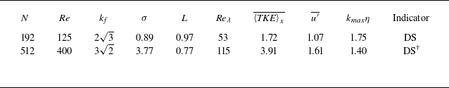
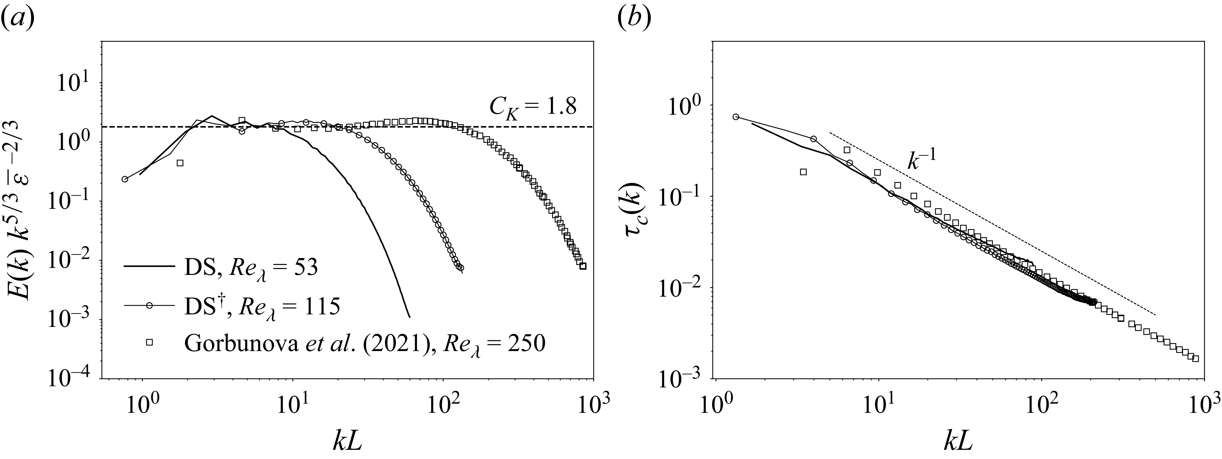


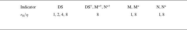


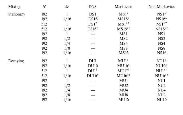


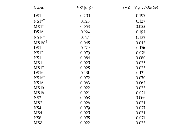


 Open access