


1. Introduction
A variety of interesting dynamic behaviours of a drop in partial contact with a solid wall, subjected to different mechanical excitations, may occur, e.g. drop atomization (James et al. Reference James, Vukasinovic, Smith and Glezer2003), formation of sub-harmonic interfacial wave patterns (Vukasinovic, Smith & Glezer Reference Vukasinovic, Smith and Glezer2007), triple modes in liquid puddles (Noblin, Buguin & Brochard-Wyart Reference Noblin, Buguin and Brochard-Wyart2005) and controllable motion of sessile drops (Noblin, Kofman & Celestini Reference Noblin, Kofman and Celestini2009b; Ding et al. Reference Ding, Zhu, Gao and Lu2018). When the forcing frequency matches one of the natural frequencies of the constrained drop, the resonance takes place. The system at resonance allows for the occurrence of the aforementioned behaviours with very little energy input. Therefore, the natural frequencies of drops are key features of the vibration phenomena, and their accurate prediction is important to our basic understanding of drop dynamics.
The earliest study of drop vibrations can date back to the pioneering work of Rayleigh (Reference Rayleigh1879). In the absence of external forces, a free drop held by surface tension assumes a spherical equilibrium shape. Owing to its simple geometry, the natural frequencies of a spherical drop can be analytically derived in the linear inviscid limit (Rayleigh Reference Rayleigh1879; Lamb Reference Lamb1932). The discrete spectrum of natural frequencies  $\omega _{[k,l]}$ is
 \begin{equation} \omega _{[k,l]}^2 = \frac{\sigma }{{\rho {R^3}}}k\left( {k - 1} \right)\left( {k + 2} \right),\quad k,l = 0,1, \ldots ,\quad l\leq k, \end{equation}
where the subscripts  $k$ and $l$ are the polar and azimuthal wavenumbers, respectively, $\sigma$ is the surface tension, $\rho$ is the drop density and $R$ is the drop radius. According to the spherical harmonic classification $[k,l]$, mode shapes are categorized as zonal ( $l=0$) for axisymmetric modes, sectoral for star-shaped modes ( $k=l>0$) and tesseral for all the other modes ( $k > l>0$). The Rayleigh–Lamb (RL) spectrum (1.1) is accurate for predicting the frequencies of small-amplitude free oscillations of spherical drops with low viscosity, which has been verified experimentally using immiscible drops by Trinh & Wang (Reference Trinh and Wang1982) and using free drops in microgravity by Wang, Anilkumar & Lee (Reference Wang, Anilkumar and Lee1996).
Further theoretical studies of the free drop problem have examined the effects of viscosity (Lamb Reference Lamb1932; Miller & Scriven Reference Miller and Scriven1968; Prosperetti Reference Prosperetti1980), finite-amplitude oscillations (Tsamopoulos & Brown Reference Tsamopoulos and Brown1983; Azuma & Yoshihara Reference Azuma and Yoshihara1999) and external forces (such as electrostatic Feng & Beard (Reference Feng and Beard1990) and isorotational fields Busse Reference Busse1984) on natural frequencies. It was found that viscous and nonlinear oscillations shift the frequency downwards from the RL spectrum (Becker, Hiller & Kowalewski Reference Becker, Hiller and Kowalewski1994). By contrast, the frequency shifts due to external forces are far more complex, as the base state of the drop is distorted by external forces. For example, the centrifugal force shifts the frequencies of axisymmetric modes either upwards or downwards, depending on whether the steady distortion leads to an oblate or prolate spheroid, respectively (Busse Reference Busse1984). The above results were experimentally verified by Annamalai, Trinh & Wang (Reference Annamalai, Trinh and Wang1985).
Unlike the free drop problem, there are generally no analytical expressions for the natural frequencies of sessile drops. For the small-amplitude oscillations, many theoretical models have been developed to predict the natural frequencies based on the normal-mode decomposition (Strani & Sabetta Reference Strani and Sabetta1984, Reference Strani and Sabetta1988; Gañán & Barrero Reference Gañán and Barrero1990; Gañán Reference Gañán1991; Lyubimov, Lyubimova & Shklyaev Reference Lyubimov, Lyubimova and Shklyaev2004, Reference Lyubimov, Lyubimova and Shklyaev2006; Bostwick & Steen Reference Bostwick and Steen2014; Sharma & Wilson Reference Sharma and Wilson2021; Ding & Bostwick Reference Ding and Bostwick2022b). These models are to solve a functional eigenvalue problem governing the linear dynamics of sessile drops (Myshkis et al. Reference Myshkis, Babskii, Kopachevskii, Slobozhanin and Tyuptsov1987, p. 281). The eigenvalues are the natural frequencies of vibration, and the eigenvectors are the shapes of these vibrational modes. The eigenvalue problem is generally difficult to solve because of the complexity of the drop configuration (including solid walls and contact lines). Strani & Sabetta (Reference Strani and Sabetta1984) used the Green's function method to solve the problem for the axisymmetric oscillations of drops supported by a spherical bowl-shaped substrate. It was found that the presence of the substrate raises the natural frequencies and induces an additional low-frequency vibration mode. Later, they extended their inviscid model to the viscous case (Strani & Sabetta Reference Strani and Sabetta1988). Gañán & Barrero (Reference Gañán and Barrero1990) used an analytical spectral method to predict the natural frequencies of the axisymmetric and non-axisymmetric modes for drops on a plane. This method was extended to drops of more general shape (Gañán Reference Gañán1991). In these studies, the contact line (CL) was considered to be pinned to model the effect of a static contact-angle hysteresis on the drops with a small oscillation amplitude.
Recent theoretical studies have focused on the role of the CL condition in modifying the frequency spectrum. There are three types of CLs: free, pinned and dynamic. The free and pinned CL conditions are to keep the contact angle and CL fixed, respectively. The dynamic CL condition (where the contact-angle deviation  $\Delta \alpha$ varies smoothly with the CL speed $u_{CL}$) yields $\Delta \alpha =\varLambda u_{CL}$ with a phenomenological constant $\varLambda$ (called the mobility parameter), referred to as the Hocking condition first introduced by Davis (Reference Davis1980). Apparently, the free and pinned CL conditions can be recovered from the Hocking condition as limiting cases for $\varLambda =0$ and $\varLambda \to \infty$, respectively. Lyubimov et al. (Reference Lyubimov, Lyubimova and Shklyaev2004, Reference Lyubimov, Lyubimova and Shklyaev2006) considered the Hocking condition for the oscillations of a hemispherical drop and examined the damping of CL dissipation. Then, Bostwick & Steen (Reference Bostwick and Steen2014) extended the results of hemispherical drops to spherical-cap base states by using a Green's function method. It was found that the free and pinned CL conditions lead to the lower and upper bounds on natural frequencies, respectively, and the Hocking condition always leads to a CL dissipation (except for the limiting cases $\varLambda =0$ and $\varLambda \to \infty$). Sharma & Wilson (Reference Sharma and Wilson2021) presented a fully analytical solution based on a toroidal analysis for the spherical-cap drop with a pinned CL. Recently, Ding & Bostwick (Reference Ding and Bostwick2022b) investigated the frequency spectrum of sessile drops under pressure constraints. The above theoretical results have compared favourably to experiments (Chang et al. Reference Chang, Bostwick, Steen and Daniel2013, Reference Chang, Bostwick, Daniel and Steen2015) and numerical simulations (Basaran & DePaoli Reference Basaran and DePaoli1994; Olgac, Izbassarov & Muradoglu Reference Olgac, Izbassarov and Muradoglu2013; Sakakeeny & Ling Reference Sakakeeny and Ling2020, Reference Sakakeeny and Ling2021; Sakakeeny et al. Reference Sakakeeny, Deshpande, Deb, Alvarado and Ling2021).
The theoretical models described above are generally restricted to spherical-cap drops. To overcome this limitation, several simple models for frequency prediction have been proposed based on modifications to the RL spectrum (1.1) (Yoshiyasu, Matsuda & Takaki Reference Yoshiyasu, Matsuda and Takaki1996; Perez et al. Reference Perez, Brechet, Salvo, Papoular and Suery1999), or on analogies to one-dimensional waves (Noblin, Buguin & Brochard-Wyart Reference Noblin, Buguin and Brochard-Wyart2004) as well as a harmonic oscillator (Celestini & Kofman Reference Celestini and Kofman2006; Sakakeeny & Ling Reference Sakakeeny and Ling2020, Reference Sakakeeny and Ling2021). However, the simple models cannot give mode shapes and are inaccurate for some drop experiments (Vukasinovic et al. Reference Vukasinovic, Smith and Glezer2007; Chang et al. Reference Chang, Bostwick, Steen and Daniel2013; Yao et al. Reference Yao, Lai, Alvarado, Zhou, Aung and Mejia2017). In view of this, we turn our attention to numerical methods to solve the eigenvalue problem governing the linear dynamics of drops, so that we can deal with small-amplitude oscillations of inviscid drops of arbitrary shape (e.g. liquid bridges and flattened sessile drops). Because the governing equation is linear, the boundary element method (BEM) is suitable for this problem, which has been widely used in the eigenvalue problem of liquid sloshing (Ebrahimian, Noorian & Haddadpour Reference Ebrahimian, Noorian and Haddadpour2013, Reference Ebrahimian, Noorian and Haddadpour2015). Indeed, the liquid sloshing in a container and the oscillations of sessile drops are mathematically the same problem, except for their different boundary shapes. So far, the BEM has only been applied to drop oscillations with pinned CLs in a microgravity environment (Siekmann & Schilling Reference Siekmann and Schilling1989). The BEM can be further exploited to investigate oscillations of drops with arbitrary shapes.
For the special case of hemispherical drops with free CLs ( $\alpha =90^{\circ }$, $\varLambda =0$, called the free semi-drop), the frequency spectrum satisfies the RL spectrum (1.1) with $k+l$ being even. The zonal, sectoral and tesseral classification of modes described earlier still holds for sessile drops. From (1.1), Lyubimov et al. (Reference Lyubimov, Lyubimova and Shklyaev2004) noted the spectral degeneracy of the free semi-drop: all modes with the same $k$ but different $l$ have the same frequency. This degeneracy can be broken by varying either the contact angle $\alpha$ (Bostwick & Steen Reference Bostwick and Steen2014) or the mobility parameter $\varLambda$ (Lyubimov et al. Reference Lyubimov, Lyubimova and Shklyaev2006). That is, the same frequencies of the degenerate modes will become different as either the contact angle changes from $\alpha =90^{\circ }$ or the mobility parameter changes from $\varLambda =0$. Another noteworthy feature of the free semi-drop is that the mode $[1,1]$ (referred to as the Noether mode by Bostwick & Steen Reference Bostwick and Steen2014) is a zero frequency mode corresponding to horizontal motion of the drop's centre of mass. However, the Noether mode tends to be ignored due to its zero frequency. Bostwick & Steen (Reference Bostwick and Steen2014) reported that the Noether mode can have a non-zero frequency by varying $\alpha$ or $\varLambda$. For instance, the CL pinning ( $\varLambda \to \infty$) increases the frequency squared $\lambda _{[1,1]}^{2}(= \omega ^2{\rho {R^3}}/\sigma )$ from zero to about $4.92$. When varying $\alpha$, Bostwick & Steen (Reference Bostwick and Steen2014) found that $\lambda _{[1,1]}^{2}>0$ for $\alpha <90^{\circ }$ and $\lambda _{[1,1]}^{2}<0$ for $\alpha >90^{\circ }$. The latter finding indicates that a super-hemispherical drop ( $\alpha >90^{\circ }$) with a free CL exhibits an instability ( $\lambda ^{2}<0$) that correlates with a horizontal centre-of-mass motion. This instability suggests a spontaneous horizontal walking of drops in practice and is therefore referred to as the ‘walking’ drop instability by Bostwick & Steen (Reference Bostwick and Steen2014). In addition, the lowest mode (with the smallest non-zero frequency) is also important in practice, as this mode is usually the first to be excited. According to the spectral ordering, the lowest mode of spherical-cap drops can be $[1,1]$, $[2,0]$ or $[2,2]$ depending on the CL condition and the contact angle (Bostwick & Steen Reference Bostwick and Steen2014). All of these results are closely related to the frequency spectrum.
Due to the limitations of the theoretical models on drop shape, the effects of gravity on the above results are not fully understood, particularly how the frequency spectrum is modified by gravity. Gravity not only flattens the sessile drop, but also introduces an additional restoring force to make the drop ‘stiffer’ in analogy to a harmonic oscillator (Perez et al. Reference Perez, Brechet, Salvo, Papoular and Suery1999). Recent numerical simulations showed that the frequencies of the first few axisymmetric modes increase with gravity in their parameter domain (Sakakeeny & Ling Reference Sakakeeny and Ling2020, Reference Sakakeeny and Ling2021). A similar downward frequency shift due to gravity was also observed for pendant drops (Basaran & DePaoli Reference Basaran and DePaoli1994). This implies that the dependence of the frequency of the axisymmetric mode on gravity seems to be monotonous. Our results, however, suggest otherwise in a wider parameter domain. With regard to non-axisymmetric oscillations, non-axisymmetric modes are usually excited sub-harmonically at half of the driving frequency as the forcing amplitude is above a threshold, while axisymmetric modes are excited harmonically at the frequency of forcing (Vukasinovic et al. Reference Vukasinovic, Smith and Glezer2007; Chang et al. Reference Chang, Bostwick, Daniel and Steen2015). Only some experiments on non-axisymmetric oscillations of sessile drops dominated by gravity have been conducted (e.g. Noblin et al. Reference Noblin, Buguin and Brochard-Wyart2005; Vukasinovic et al. Reference Vukasinovic, Smith and Glezer2007; Noblin, Buguin & Brochard-Wyart Reference Noblin, Buguin and Brochard-Wyart2009a). Their main concern is the critical forcing amplitude for the transition from axisymmetric to non-axisymmetric oscillations. The effects of gravity on high-order modes and non-axisymmetric modes have not been symmetrically studied in detail. Moreover, a lot of experiments of drop vibrations on Earth are dominated by gravity, so one needs a model that covers this aspect. The present work will develop a numerical model based on the BEM that solves the eigenvalue problem for the oscillations of sessile drops in the presence of gravity (figure 1a). After validating the results of spherical-cap drops with free and pinned CLs, we focus on the frequency shifts due to gravity for sessile drops, depending on the CL conditions (free or pinned) and its equilibrium contact angle.
(a) Schematic diagram of a sessile drop with contact angle  $\alpha$ sitting on a plane under gravity $g$. The drop is flattened by gravity, whereas its equilibrium shape without gravity is a spherical cap (dashed line). (b,c) The perturbed $\bar \varGamma$ and unperturbed $\varGamma$ surfaces (b) in cylindrical coordinates $( {r,\varphi,z} )$ with a curvilinear coordinate $s$ and (c) in three-dimensional Cartesian coordinates. Here $\eta$ is the perturbation of the liquid free surface. At the CL $\gamma$ (red point in b) there is a free or pinned CL condition to restrict the perturbation $\eta$.

As mentioned earlier, the walking instability of hydrophobic drops is inferred by Bostwick & Steen (Reference Bostwick and Steen2014) from the negative eigenvalue squared of the  $[1,1]$ mode. Physically, the walking drop instability, analogous to the Rayleigh–Plateau instability (Bostwick & Steen Reference Bostwick and Steen2018; Wang & Tao Reference Wang and Tao2022), should be a capillary instability driven by a surface energy gradient, leading to a surface reconfiguration according to the shape of the instability mode. Since the $[1,1]$ mode corresponds to a drop translation, the walking drop instability exhibits a horizontal drop movement. Note that this horizontal movement should be spontaneous and is different from the directional movement of the drop due to the parametric instability (see e.g. Ding et al. Reference Ding, Zhu, Gao and Lu2018; Costalonga & Brunet Reference Costalonga and Brunet2020). Recently, several relevant instabilities have been reported in some theoretical literature (Bostwick & Steen Reference Bostwick and Steen2018; Steen, Chang & Bostwick Reference Steen, Chang and Bostwick2019; Ding & Bostwick Reference Ding and Bostwick2022a,Reference Ding and Bostwickb). The walking drop instability is also illustrated by energy analysis by Bostwick & Steen (Reference Bostwick and Steen2014). However, a drop with a free CL on a plane does not possess any energy gradient leading to instability and should have horizontal translational invariance. This suggests that the walking drop instability cannot exist and the corresponding eigenvalue should be zero. In this work, the eigenvalue of the Noether mode $[1,1]$ is of particular concern from numerical and theoretical perspectives.
The paper is organized as follows. In § 2 we write the linearized governing equations and boundary conditions to generate a functional eigenvalue problem for natural oscillations of sessile drops with free or pinned CLs. In § 3 a model based on the BEM is developed to numerically solve the eigenvalue problem for determining the natural frequencies and corresponding mode shapes. In § 4 numerical results are compared with theoretical and experimental results to confirm the model, and then the frequency shifts due to gravity are examined. In § 5 we discuss some fascinating consequences of the frequency shifts. Finally, in § 6 the paper is summarized and the conclusions are presented.
2. Mathematical formulation
Consider a sessile drop of contact angle  $\alpha$ sitting on a plane under gravity $g$, as shown in figure 1(a). To establish the vibration model, we follow the theoretical framework set forth in Myshkis et al. (Reference Myshkis, Babskii, Kopachevskii, Slobozhanin and Tyuptsov1987) for oscillations of capillary surfaces in an external force field. Two assumptions are made: (i) the liquid is assumed to be incompressible and ideal so that the potential flow theory can be used; (ii) the small-amplitude oscillations are considered, i.e. the velocity, the deformation of the free surface and their derivatives are infinitesimal quantities. Therefore, only linear terms are retained and the higher-order terms are neglected. The linear assumption allows us to consider the fluid domain $D$ to remain unchanged for small perturbations (figure 1b).
2.1. Governing equations and boundary conditions
In the fluid domain  $D$, based on the potential flow theory, the velocity field $\boldsymbol {u}$ can be described by $\boldsymbol {u} = - \boldsymbol {\nabla } \psi$, where $\psi$ is the velocity potential function. As a result of continuity ( $\boldsymbol {\nabla } \boldsymbol{\cdot } \boldsymbol {u} = 0$), the potential function has to satisfy Laplace's equation,
 \begin{equation} {\nabla^2}\psi = 0\quad [D]. \end{equation}
 On the free surface  $\partial {D^f}$, there are two boundary conditions. The first is the free-surface kinematic condition, given by
 \begin{equation} \frac{{\partial \psi }}{{\partial n}} ={-} \frac{{\partial \eta }}{{\partial t}}\quad [\partial {D^f}], \end{equation}
where  $\boldsymbol {n}$ is the normal unit vector directed out of the fluid domain and $\eta$ is the perturbation of the free surface. The kinematic condition (2.2) means that the normal velocity ${u_n} = - {{\partial \psi } /{\partial n}}$ on the surface coincides with the perturbation velocity. In the linear potential theory, the pressure is only related to the potential, expressed by the linearized Bernoulli equation
 \begin{equation} \frac{{\partial \psi }}{{\partial t}} - \frac{p}{\rho } - \varPi = 0, \end{equation}
where  $\varPi = gz$ is the gravitational potential.
The second condition on the free surface is the Young–Laplace equation that relates the mean curvature and the pressure difference,
 \begin{equation} 2\sigma \bar H ={-} p\quad [\partial {D^f}], \end{equation}
where  $\bar H$ is the mean curvature of the perturbed surface $\bar \varGamma$. We consider the Bernoulli equation (2.3) on $\bar {\varGamma }$ and then substitute the linear form of (2.4) into (2.3) to obtain the dynamic pressure balance (Myshkis et al. Reference Myshkis, Babskii, Kopachevskii, Slobozhanin and Tyuptsov1987, p. 280)
 \begin{equation} \frac{{\partial \psi }}{{\partial t}} + \frac{\sigma }{\rho }[{\varDelta _\varGamma }\eta + ({k_1}^2 + {k_2}^2)\eta ] - \frac{{\partial \varPi }}{{\partial n}}\eta = 0\quad [\partial {D^f}], \end{equation}
where  ${\varDelta _\varGamma }$ is the Laplace–Beltrami operator depending on the equilibrium shape $\varGamma$, and ${k_1}$, ${k_2}$ are the two principle curvatures of $\varGamma$. It is worth noting that the sign of the two principal curvatures of the axisymmetric drop surface $\varGamma$ depends only on the direction of the normal vector of the liquid surface, and here $k_1$ and $k_2$ have negative signs (see Appendix A).
On the solid surface  $\partial {D^s}$, there is a no-penetration condition,
 \begin{equation} \frac{{\partial \psi }}{{\partial n}} = 0\quad [\partial {D^s}]. \end{equation}
 At the CL  $\gamma$, there is a CL condition,
 \begin{equation} \frac{{\partial \eta }}{{\partial e}} + \chi \eta = 0\quad [\gamma ]. \end{equation}
where  $\boldsymbol {e}$ is a unit vector normal to $\gamma$ in a plane tangential to $\varGamma$ (directed out of the free surface $\varGamma$) and $\chi$ is a boundary parameter depending on the geometry at the CL. For the axisymmetric case, the expression of $\chi$ will be given in § 2.4.
Additionally, the perturbation has to satisfy the condition of volume conservation
 \begin{equation} \int_{\varGamma} {\eta \,{\rm{d}}\varGamma } = 0\quad [\partial {D^f}]. \end{equation}
The system of equations and boundary conditions (2.1), (2.2), (2.5)–(2.8) governs the natural oscillations of sessile drops under gravity and can be further reduced to a functional eigenvalue problem (see § 2.3).
2.2. Dimensionless analysis in cylindrical coordinates
We scale all of the drop volumes by  $v_{*} = {3\tilde {v}}/{2{\rm \pi} }$ to compare with the hemispherical drop, where $\tilde {v}$ is the drop volume. As a consequence, the dimensionless volume, ${v} \equiv \tilde {v}/{v_{*}}$, of all the cases is kept constant at $2{\rm \pi} /3$, which is equal to the volume of a hemisphere of radius one, thereby excluding the volume effects. Therefore, the characteristic length is $l_{*} = {{v_*}^{1/3}}$. Accordingly, we introduce the following characteristic time and potentials:
 \begin{equation} {t_ * } = \sqrt {\rho {{l_ *}^3}/\sigma } , \quad {\psi _ * } = {{l_ *}^2}/{t_ * }, \quad {\varPi _ * } = {\left( {l_ */{t_ * }} \right)^2}. \end{equation}
Then, in dimensionless forms, the governing equations and boundary conditions (2.1), (2.2), (2.5)–(2.8) are rewritten as
 \begin{gather} {\nabla ^2}\psi = 0\quad [D], \end{gather}
 \begin{gather}\frac{{\partial \psi }}{{\partial n}} = 0\quad [\partial {D^s}], \end{gather}
 \begin{gather}\frac{{\partial \psi }}{{\partial n}} ={-} \frac{{\partial \eta }}{{\partial t}}\quad [\partial {D^f}], \end{gather}
 \begin{gather}\frac{{\partial \psi }}{{\partial t}} + {\varDelta _\varGamma }\eta + ({k_1}^2 + {k_2}^2)\eta - Bo \frac{{\partial z}}{{\partial n}}\eta = 0\quad [\partial {D^f}], \end{gather}
 \begin{gather}\int_{\varGamma} {\eta \,{\rm{d}}\varGamma } = 0\quad [\partial {D^f}], \end{gather}
 \begin{gather}\frac{{\partial \eta }}{{\partial e}} + \chi \eta = 0\quad [\gamma ], \end{gather}
where the Bond number is defined as
 \begin{equation} Bo \equiv \frac{\rho g {l_*}^{2}}{\sigma} =\frac{\rho g }{\sigma}\left(\frac{3\tilde{v}}{2{\rm \pi}}\right)^{2 / 3}. \end{equation}
 In the cylindrical coordinates  $({r,\varphi,z} )$ with a curvilinear coordinate $s$ (see figure 1b), the two principle curvatures ( ${k_1}, {k_2}$) and the operators ( ${\nabla ^2}$, ${\varDelta _\varGamma }$) for the system (2.10) are, respectively,
 \begin{gather} {k_1} = Bo \times z - \frac{{\sin \beta }}{r} + \mu, \end{gather}
 \begin{gather}{k_2} = \frac{{\sin \beta }}{r}, \end{gather}
 \begin{gather}{\nabla ^2}\psi = \frac{1}{r}\frac{\partial }{{\partial r}}\left( {r\frac{{\partial \psi }}{{\partial r}}} \right) + \frac{1}{{{r^2}}}\frac{{{\partial ^2}\psi }}{{\partial {\varphi ^2}}} + \frac{{{\partial ^2}\psi }}{{\partial {z^2}}}, \end{gather}
 \begin{gather}{\varDelta _\varGamma }\eta = \frac{{{\partial ^2}\eta }}{{\partial {s^2}}} + \frac{1}{r}\frac{{{\rm{d}}r}}{{{\rm{d}}s}}\frac{{\partial \eta }}{{\partial s}} + \frac{1}{{{r^2}}}\frac{{{\partial ^2}\eta }}{{\partial {\varphi ^2}}}, \end{gather}
where  $\beta$ is the inclination angle of the free surface, $\mu$ is a Lagrange multiplier whose value is equal to twice the mean curvature of the drop apex, and the drop equilibrium shape $\varGamma :=(r(s),z(s))$ is the base state of the vibration problem. The static equilibrium shape of sessile drops in the presence of gravity has been studied extensively (e.g. Padday Reference Padday1971; Del Rıo & Neumann Reference Del Rıo and Neumann1997). The numerical method for determining the drop shape is given in Appendix B.
There are only two independent parameters for the drop configuration, namely the contact angle  $\alpha$ and the Bond number $Bo$. Note that all variables considered here and in what follows are dimensionless and retain their original notations for convenience.
2.3. Reduction to eigenvalue problem
Normal modes of  $\psi$ and $\eta$ in cylindrical coordinates are written as (see e.g. Bostwick & Steen Reference Bostwick and Steen2014)
 \begin{equation} \psi (\boldsymbol{x},t) = \phi (r,z){\mathrm{e}^{{\rm i}\lambda t}}{\mathrm{e}^{{\rm i}l\varphi }} \quad {\rm{and}} \quad \eta (s,\varphi ,t) = y(s){\mathrm{e}^{{\rm i}\lambda t}}{\mathrm{e}^{{\rm i}l\varphi }}, \end{equation}
respectively, where  $\lambda \equiv \omega t^{*}$ is the scaled frequency and $l$ is the azimuthal wavenumber.
Applying (2.13) to (2.10) with (2.12), we obtain the functional eigenvalue problem governing the linear dynamics of drops,
 \begin{gather} \frac{1}{r}\frac{\partial }{{\partial r}}\left( {r\frac{{\partial \phi }}{{\partial r}}} \right) + \frac{{{\partial ^2}\phi }}{{\partial {z^2}}} - \frac{{{l^2}}}{{{r^2}}}\phi = 0\quad [D], \end{gather}
 \begin{gather}\frac{{\partial \phi }}{{\partial n}} = 0\quad [\partial {D^s}], \end{gather}
 \begin{gather}{\left( {\frac{{\partial \phi }}{{\partial n}}} \right)^{\prime \prime }} + \frac{{r'}}{r}{\left( {\frac{{\partial \phi }}{{\partial n}}} \right)^\prime } - \left[ {Bo \times r' - \left( {{k_1}^2 + {k_2}^2} \right) + \frac{{{l^2}}}{{{r^2}}}} \right]\frac{{\partial \phi }}{{\partial n}} ={-} {\lambda ^2}\phi \quad [\partial {D^f}], \end{gather}
 \begin{gather}\int_{\varGamma} {\frac{{\partial \phi }}{{\partial n}}{\rm{d}}\varGamma } = 0\quad [\partial {D^f}], \end{gather}
 \begin{gather}{\left. {{{\left( {\frac{{\partial \phi }}{{\partial n}}} \right)}^\prime } + \chi \frac{{\partial \phi }}{{\partial n}} = 0} \right|_{s = {s_c}}}\quad [\gamma ]. \end{gather}
 Equation (2.14a) is Laplace's equation written in cylindrical coordinates  $(r,z)$, (2.14b) is the no-penetration condition on the solid surface and (2.14d) is the condition of volume conservation. Equation (2.14c) is the free-surface governing equation derived from the kinematic condition (2.10c) and the dynamic pressure balance (2.10d), where the prime refers to the derivative with respect to $s$. Equation (2.14e) is the CL condition, where $s_c$ is the arc length at the CL.
2.4. Contact line conditions
In (2.14e) the boundary parameter is given by (Myshkis et al. Reference Myshkis, Babskii, Kopachevskii, Slobozhanin and Tyuptsov1987, p. 126)
 \begin{equation} \chi = {\frac{{{k_1}(s_c)\cos \alpha - \tilde k}}{{\sin \alpha }}}, \end{equation}
where  $\tilde k$ is the curvature of the solid surface at the CL $s = {s_c}$.
Two types of CL conditions are considered in this work: ‘free’ and ‘pinned’. The free CL condition is to preserve the contact angle during motion, and the solid surface is considered to be ideally smooth so that  $\tilde {k} = 0$ for the planar substrate. Therefore, for the free CL condition, the boundary parameter is
 \begin{equation} \chi = {{k_1}(s_c)\cot \alpha } . \end{equation}
 For a spherical cap with a contact radius of 1 (i.e. with a signed curvature  ${k_1} = - \sin \alpha$), the boundary parameter can further reduce to $\chi = - \cos \alpha$, which recovers the free CL condition in Bostwick & Steen (Reference Bostwick and Steen2014) except for having a minus sign for $\cos \alpha$. This minus sign will lead us to different results, in particular regarding whether the walking drop instability reported in Bostwick & Steen (Reference Bostwick and Steen2014) exists, as will be discussed in detail in § 5.1.
For the pinned CL condition, the boundary parameter is (Myshkis et al. Reference Myshkis, Babskii, Kopachevskii, Slobozhanin and Tyuptsov1987)
 \begin{equation} \chi \to { + \infty } . \end{equation}
Substituting (2.16) and (2.17) into (2.14e), we obtain the free CL condition,
 \begin{equation} {\left. {{{\left( {\frac{{\partial \phi }}{{\partial n}}} \right)}^\prime } + {k_1}\cot \alpha \frac{{\partial \phi }}{{\partial n}} = 0} \right|_{s = {s_c}}}, \end{equation}
and the pinned CL condition,
 \begin{equation} {\left. {\frac{{\partial \phi }}{{\partial n}} = 0} \right|_{s = {s_c}}}, \end{equation}
respectively.
3. Boundary element method model
In this section we introduce how to apply the BEM to solve the eigenvalue problem (2.14) for a given equilibrium shape  $\varGamma$ (figure 1b) to obtain the natural frequencies and corresponding mode shapes. As mentioned in § 1, the classical theoretical methods to this problem (e.g. Lyubimov et al. Reference Lyubimov, Lyubimova and Shklyaev2006; Bostwick & Steen Reference Bostwick and Steen2014; Sharma & Wilson Reference Sharma and Wilson2021) require the drop shape to be a hemisphere or a spherical cap, which are difficult to be extended to drops of flattened shape. Compared with the theoretical methods, the BEM can deal with arbitrary geometry and is therefore applicable to our problem. The key idea is to establish the relationship between the velocity potential $\phi$ and its normal derivative ${{\partial \phi }}/{{\partial n}}$ on the boundary through a boundary integral equation, so as to construct a generalized matrix eigenvalue problem.
The BEM is widely applied to potential flow problems governed by the Laplace equation (2.14a) (Pozrikidis Reference Pozrikidis2002). However, there are relatively few models based on the BEM for modal analysis of free interfaces. To our knowledge, two major axisymmetric BEM (hereafter referred to as axiBEM) models for axisymmetric problems have been developed by Siekmann & Schilling (Reference Siekmann and Schilling1989) and Ebrahimian et al. (Reference Ebrahimian, Noorian and Haddadpour2013, Reference Ebrahimian, Noorian and Haddadpour2015), respectively. The first model is based on the indirect formulation of axiBEM, whereas the latter uses the direct formulation. The direct formulation utilizes the velocity potential and its normal derivative as solutions, whereas the solution of the indirect formulation is a distribution of singularities that has no physical significance (Pozrikidis Reference Pozrikidis2002). Therefore, our model takes the more intuitive direct formulation of Ebrahimian et al. (Reference Ebrahimian, Noorian and Haddadpour2013, Reference Ebrahimian, Noorian and Haddadpour2015).
3.1. Discretization of boundary integral equation
The BEM has the advantage of reducing the overall dimension by one and, thus, we only need to deal with the problem on the boundary. Here we follow Ebrahimian et al. (Reference Ebrahimian, Noorian and Haddadpour2013, Reference Ebrahimian, Noorian and Haddadpour2015) and adopt the standard axiBEM formulation (Pozrikidis Reference Pozrikidis2002) to construct a system of linear equations.
3.1.1. Boundary integral equation
On the boundary  $\partial D$, the velocity potential $\phi$ and its normal derivative ${{\partial \phi }}/{{\partial n}}$ are related by the boundary integral equation (Pozrikidis Reference Pozrikidis2002)
 \begin{equation} \frac{1}{2}\phi ({\boldsymbol{x}_0}) = \int_{\partial {D}} {\left[ {{G^l}(\boldsymbol{x},{\boldsymbol{x}_0})\frac{{\partial \phi }}{{\partial n}}(\boldsymbol{x}) - \frac{{\partial {G^l}(\boldsymbol{x},\boldsymbol{x}_0)}}{{\partial n}}\phi (\boldsymbol{x})} \right]r\,\mathrm{d}s(\boldsymbol{x})}, \end{equation}
where  ${\boldsymbol {x}_0} = ({r_0},{z_0})$ and $\boldsymbol {x} = (r,z)$ are the coordinates of the source point and the field point on the boundary, respectively. In (3.1), ${G^l}(\boldsymbol {x},{\boldsymbol {x}_0})$ is the axisymmetric free-space Green's function of (2.14 $a$) for a given azimuthal wavenumber $l$, given as (for a detailed derivation, see Appendix C)
 \begin{equation} {G^l}(\boldsymbol{x},{\boldsymbol{x}_0}) = \frac{1}{{{\rm \pi} \sqrt {{{\left( {z - {z_0}} \right)}^2} + {{\left( {r + {r_0}} \right)}^2}} }}\int_0^{{\rm \pi} /2} {\frac{{\cos (2l\varsigma )\,\mathrm{d}\varsigma }}{{\sqrt {1 - {k^2}{{\cos }^2}\varsigma } }}} ,\quad l = 0,1,\ldots, \end{equation}
with
 \begin{equation} {k^2} = \frac{{4r{r_0}}}{{{{\left( {z - {z_0}} \right)}^2} + {{\left( {r + {r_0}} \right)}^2}}}. \end{equation}
When  $l = 0$, the Green's function (3.2) can be reduced to the Green's function of Laplace's equation in the axisymmetric problem (Pozrikidis Reference Pozrikidis2002, p. 108).
Equation (3.1) defined on the boundary  $\partial D$ is a reformulation of Laplace's equation (2.14a) and can be further discretized on the boundary $\partial D$.
3.1.2. Boundary discretization
The boundary  $\partial D = \partial {D^f} + \partial {D^s}$ is discretized by line elements with straight or curved shapes (figure 2). The free-surface elements $\partial {D_i}$, $i = 1,2,\ldots,N$ are defined by clamped-end cubic splines, while the wall elements $\partial {D_i}$, $i = N + 1,N + 2,\ldots,N + M$ are straight lines. Based on the cubic spline interpolation, we obtain the approximate analytical expression for each free-surface element,
 \begin{equation} \left. {\begin{array}{c@{}} {{r_i}(\xi ) = {d_i} + {a_i}\xi + {b_i}{\xi ^2} + {c_i}{\xi ^3}} \\ {{z_i}(\xi ) = {{\bar{d}}_i} + {{\bar{a}}_i}\xi + {{\bar{b}}_i}{\xi ^2} + {{\bar{c}}_i}{\xi ^3}} \end{array}} \right\}\quad {\rm{on}}\ \partial {D_i},\quad i = 1,2,\ldots,N, \end{equation}
with a change of variables  $s = {{\Delta s}}/{2}( {\xi + 2i - 1} )$ so $\xi \in [ - 1,1]$, where $( {{d_i},{{\bar {d}}_i}} )$ is the location of the midpoint ${P_i}$ and $\Delta s = {s_c}/N$ is the length of the free-surface element. The algorithm for computing clamped-end cubic splines is well known (see e.g. Pozrikidis Reference Pozrikidis2002, pp. 56–60). Here the eight coefficients ${a_i}$, ${b_i}$,…, ${\bar {d}_i}$ are calculated by using the MATLAB function ‘spline’, where the nodes ${Q_i}$, $i = 1,2,\ldots,N+1$ for the cubic spline interpolation are determined by numerically solving the Young–Laplace equation (Appendix B).
Discretization of the boundary  $\partial D = \partial {D^f} + \partial {D^s}$ into a collection of cubic spline elements $\partial {D_i}$, $i = 1,2,\ldots,N$ for $\partial {D^f}$ and straight line elements $\partial {D_i}$, $i = N + 1,N + 2,\ldots,N + M$ for $\partial {D^s}$. The midpoints of elements $\partial {D_i}$ denoted by ${P_i}$ serve as collocation points for the collocation method. Here, the boundaries $\partial {D^f}$ and $\partial {D^s}$ are uniformly divided, respectively. Thus, the length of each free-surface element is $\Delta s = {s_c}/N$.

In this model, we adopt the simplest approximation: the boundary distribution of  $\phi (\boldsymbol {x})$ and its normal derivative ${{\partial \phi }}/{{\partial n}}(\boldsymbol {x})$ are assumed to be constant functions on each element $\partial {D_j}$, $j = 1,2,\ldots,N + M$, denoted respectively by ${\phi _j}$ and $\phi _j^ *$. Approximating the boundary integral equation (3.1) with the sum of integrals over the boundary elements, we obtain the discretized boundary integral equation,
 \begin{equation} \frac{1}{2}\phi ({\boldsymbol{x}_0}) = \sum_{j=1}^{N + M} {a_j^l({\boldsymbol{x}_0})\phi _j^ * } - \sum_{j=1}^{N + M} {b_j^l({\boldsymbol{x}_0}){\phi _j}}, \end{equation}
with the influence coefficients
 \begin{equation} \left. \begin{gathered} {a_j^l({\boldsymbol{x}_0}) = \displaystyle\int_{\partial {D_j}} {{G^l}(\boldsymbol{x},{\boldsymbol{x}_0})r\,\mathrm{d}S(\boldsymbol{x}),} }\\ {b_j^l({\boldsymbol{x}_0}) = \displaystyle\int_{\partial {D_j}} {\dfrac{{\partial {G^l}(\boldsymbol{x},{\boldsymbol{x}_0})}}{{\partial n}}r\,\mathrm{d}S(\boldsymbol{x}).} } \end{gathered}\right\} \end{equation}
 Using the midpoints  ${P_i}$ of boundary elements (see figure 2) as collocation points (i.e. letting every point ${P_i}$ be the source point $\boldsymbol {x}_0$), denoted by $\boldsymbol {x}_i^P$, for (3.5), we obtain a set of algebraic equations,
 \begin{equation} K_{ij}^l\phi _j^ * = H_{ij}^l{\phi _j}, \end{equation}
with the influence matrixes
 \begin{equation} K_{ij}^l = a_j^l(\boldsymbol{x}_i^P) \quad {\rm{and}} \quad H_{ij}^l = b_j^l(\boldsymbol{x}_i^P) + \tfrac{1}{2}{\delta _{ij}},\end{equation}
where  ${\delta _{ij}}$ is Kronecker's delta. The corresponding vector form of (3.7) is
 \begin{equation} {\boldsymbol{{K}}^l} {\boldsymbol{\phi} ^ * } = {\boldsymbol{{H}}^l} \boldsymbol{\phi}. \end{equation}
 The non-diagonal matrix coefficients of  ${\boldsymbol {{K}}^l}$ and ${\boldsymbol {{H}}^l}$ can be calculated by the Gaussian quadrature. However, the computation of diagonal coefficients $K_{ii}^l$ and $H_{ii}^l$ involves the numerical evaluation of improper integrals with singular integrands ${G^l}(\boldsymbol {x},{\boldsymbol {x}_0})$ and ${{\partial {G^l}(\boldsymbol {x},{\boldsymbol {x}_0})}}/{{\partial n}}$ (when the field point $\boldsymbol {x}$ approaches $\boldsymbol {x}_0$), which need special numerical techniques to ensure accuracy, such as subtracting out the singularity and then approximating the integral term by a Gaussian quadrature (called the subtraction singularity technique) (Pozrikidis Reference Pozrikidis2002, p. 72).
An important feature of (3.9) arising from the BEM formulation is that the influence matrixes  ${\boldsymbol {{K}}^l}$ and ${\boldsymbol {{H}}^l}$ depend only on the geometry of $\partial D$. This means that we can determine the influence matrixes only according to the drop shape $\varGamma$ without knowing other conditions.
By distinguishing the flow boundaries into free-surface and wall elements, (3.9) can be recast as
 \begin{equation} \left[\begin{array}{cc} \boldsymbol{K}_{11}^{l} & \boldsymbol{K}_{12}^{l} \\ \boldsymbol{K}_{21}^{l} & \boldsymbol{K}_{22}^{l} \end{array}\right]\left\{\begin{array}{c} \boldsymbol{\phi}_{L}^{*} \\ \boldsymbol{\phi}_{S}^{*} \end{array}\right\}=\left[\begin{array}{cc} \boldsymbol{H}_{11}^{l} & \boldsymbol{H}_{12}^{l} \\ \boldsymbol{H}_{21}^{l} & \boldsymbol{H}_{22}^{l} \end{array}\right]\left\{\begin{array}{c} \boldsymbol{\phi}_{L} \\ \boldsymbol{\phi}_{S} \end{array}\right\}, \end{equation}
where the subscripts  $L$ and $S$ denote the liquid and solid surface, respectively, and $\boldsymbol {K}_{mn}^{l}$ and $\boldsymbol {H}_{mn}^{l}$ ( $m,n = 1,2$) are the associated blocks of the influence matrixes. Note that so far we have not used any conditions other than Laplace's equation (2.14a).
3.2. Discretization of free-surface governing equation
In the present study, the free-surface governing equation defined in curvilinear coordinates is discretized into a system of linear equations using the finite difference method (similar to Ebrahimian et al. Reference Ebrahimian, Noorian and Haddadpour2015). Then the CL condition is integrated into the above system of linear equations by the ghost point method (instead of via left/right finite difference formulas as in the Ebrahimian et al.'s model). The ghost point strategy enables the central differencing scheme to be used for all finite differences, thus ensuring higher accuracy.
Using the fourth-order central finite difference schemes for  ${( {{{\partial \phi }}/{{\partial n}}} )^{\prime \prime }}$ and ${( {{{\partial \phi }}/{{\partial n}}} )^\prime }$ on the free surface (see figure 2), the discretization of (2.14c) can be written in a matrix form
 \begin{equation} \tilde{\boldsymbol{K}}^{l} \boldsymbol{\phi}_{L}^{*}={-}\lambda^{2} \boldsymbol{I} \boldsymbol{\phi}_{L}, \end{equation}
where  $\boldsymbol {I}$ is the identity matrix. Here, $\tilde {\boldsymbol {K}}^{l}$ corresponds to the linear operator on the left-hand side of (2.14c), given by
 \begin{equation} \tilde K_{ij}^l = {A_{ij}} + \frac{{{n_r}({s_i})}}{{r({s_i})}}{B_{ij}} - \left[ {Bo \times {n_r}({s_i}) - ({k_1}{{({s_i})}^2} + {k_2}{{({s_i})}^2}) + \frac{{{l^2}}}{{r{{({s_i})}^2}}}} \right]{\delta _{ij}}. \end{equation}
In (3.12),  ${s_i}$ is the arc length at ${P_i}$, ${n_r}$ is the radial component of the normal unit vector $\boldsymbol {n}$ on $\partial {D}$, and the coefficients ${A_{ij}}$ and ${B_{ij}}$ are given respectively by (see Appendix D for derivation)
 \begin{gather} {\boldsymbol{A}}=\frac{1}{12 \Delta s^{2}}\left[\begin{array}{ccccccc} C_{1,1}^{A} & C_{1,2}^{A} & -1 & & & & \\ C_{2,1}^{A} & -30 & 16 & -1 & & & \\ -1 & 16 & -30 & 16 & -1 & & \\ & \ddots & \ddots & \ddots & \ddots & \ddots & \\ & & -1 & 16 & -30 & 16 & -1 \\ & & & -1 & 16 & -30 & C_{N-1, N}^{A} \\ & & & & -1 & C_{N, N-1}^{A} & C_{N, N}^{A} \end{array}\right], \end{gather}
 \begin{gather}{\boldsymbol{B}}=\frac{1}{12 \Delta s}\left[\begin{array}{ccccccc} C_{1,1}^{B} & C_{1,2}^{B} & -1 & & & & \\ C_{2,1}^{B} & 0 & 8 & -1 & & & \\ 1 & -8 & 0 & 8 & -1 & & \\ & \ddots & \ddots & \ddots & \ddots & \ddots & \\ & & 1 & -8 & 0 & 8 & -1 \\ & & & 1 & -8 & 0 & C_{N-1, N}^{B} \\ & & & & 1 & C_{N, N-1}^{B} & C_{N, N}^{B} \end{array}\right]. \end{gather}
 There are still twelve coefficients  ${C^A}$ and ${C^B}$ to be determined in (3.13), which are located at the top left and bottom right corners of the matrices $\boldsymbol {A}$ and $\boldsymbol {B}$. The values of the undetermined coefficients depend on the type of the CL condition and whether the azimuthal wavenumber $l$ is even or odd (table 1). In this way, the free (2.18) or pinned (2.19) CL condition is incorporated in (3.11) by taking the corresponding values of coefficients ${C^A}$ and ${C^B}$ presented in table 1.
Coefficients  ${C^A}$ and ${C^B}$ in the matrixes $\boldsymbol {A}$ and $\boldsymbol {B}$ depend on the type of the CL condition and whether the azimuthal wavenumber $l$ is even or odd. For the free CL condition, ${\varepsilon _1} = {{(2 - \Delta s\chi )}}/{{(2 + \Delta s\chi )}}$ and ${\varepsilon _2} = {{(2 - 3\Delta s\chi )}}/{{(2 + 3\Delta s\chi )}}$ with $\chi$ being given in (2.16). The subscript of coefficients indicates the position in the matrix. For example, the subscript ‘2,1’ in (3.13) denotes the position $(2,1)$, i.e. the row 2 and the column 1 of the matrix. The derivation is provided in Appendix D.

3.3. Generalized matrix eigenvalue problems for natural oscillations
Until now, we have obtained two sets of linear algebraic equations (3.10) and (3.11), corresponding, respectively, to Laplace's equation (2.14a) and the free-surface governing equation (2.14c) with the free (2.18) or pinned (2.19) CL condition being incorporated. In this section we utilize the discrete form of the yet-unused condition (2.14b) to assemble (3.10) and (3.11) into a generalized matrix eigenvalue problem in a similar way to Ebrahimian et al. (Reference Ebrahimian, Noorian and Haddadpour2015). To eliminate the non-physical volume mode  $\{1,0\}$, we additionally impose the volume conservation condition (2.14d) by projecting the problem to the null space of the constraint (Porcelli et al. Reference Porcelli, Binante, Girardi, Padovani and Pasquinelli2015). Its solution gives the natural frequencies and corresponding mode shapes for a given azimuthal wavenumber $l$.
$l$.
The discrete forms of the no penetration condition (2.14b) and the volume conservation condition (2.14d) can be written as, respectively,
 \begin{gather} \boldsymbol{\phi} _S^ * = \boldsymbol{0}, \end{gather}
 \begin{gather}{{\boldsymbol{r}}_L}\boldsymbol{\phi}_L^ * = 0\quad \mbox{for} \ l=0, \end{gather}
where  ${\boldsymbol {r}_L} = \{{r({s_1})}\ \dots \ {r({s_N})}\}$ with $N$ being the number of free-surface elements.
For non-axisymmetric modes ( $l \ne 0$), the volume conservation condition is naturally satisfied. Substituting (3.14a) into (3.10) yields
 \begin{equation} \left[\boldsymbol{H}_{12}^{l}\left(\boldsymbol{H}_{22}^{l}\right)^{{-}1} \boldsymbol{K}_{21}^{l}-\boldsymbol{K}_{11}^{l}\right] \boldsymbol{\phi}_{L}^{*}=\left[\boldsymbol{H}_{12}^{l}\left(\boldsymbol{H}_{22}^{l}\right)^{{-}1} \boldsymbol{H}_{21}^{l}-\boldsymbol{H}_{11}^{l}\right] \boldsymbol{\phi}_{L}. \end{equation}
Combining (3.11) and (3.15), we have the matrix eigenvalue problem for  $l \geq 1$,
 \begin{equation} \boldsymbol{X} \boldsymbol{\phi}_{L}^{*}=\lambda^{2} \boldsymbol{Y} \boldsymbol{\phi}_{L}^{*}, \end{equation}
with
 \begin{gather} {\boldsymbol{X}}=\left[{\boldsymbol{H}}_{11}^{l}-{\boldsymbol{H}}_{12}^{l}\left( {\boldsymbol{H}}_{22}^{l}\right)^{{-}1} {\boldsymbol{H}}_{21}^{l}\right] \tilde{{\boldsymbol{K}}}^{l}, \end{gather}
 \begin{gather}{\boldsymbol{Y}}=\left[{\boldsymbol{H}}_{12}^{l}\left({\boldsymbol{H}}_{22}^{l}\right)^{{-}1} {\boldsymbol{K}}_{21}^{l}-{\boldsymbol{K}}_{11}^{l}\right]. \end{gather}
For axisymmetric modes ( $l = 0$), the eigenvalue problem (3.16) is also subject to the volume conservation condition (3.14b). The linear constraint (3.14b) can be imposed by suitably transforming this constrained problem into a modified unconstrained eigenvalue problem (Porcelli et al. Reference Porcelli, Binante, Girardi, Padovani and Pasquinelli2015). The transformation consists of projecting the eigenvalue problem (3.16) into the constraint space by explicitly constructing a basis for the null space $N ({{\boldsymbol {r}_L }} )$ of $\boldsymbol {r}_L$. For $\boldsymbol {\phi }_{L}^{*}\in N({{\boldsymbol {r}_L }} )$, let $\boldsymbol {v}$ be such that
 \begin{equation} \boldsymbol{\phi}_{L}^{*}= \boldsymbol{Z} \boldsymbol{v}, \end{equation}
where  $\boldsymbol {Z}$ is the matrix whose columns span the null space $N({{\boldsymbol {r}_L }} )$. Then, we obtain the equivalent unconstrained formulation of problem (3.16) subject to (3.14b),
 \begin{equation} \boldsymbol{Z}^{{T}} \boldsymbol{X Z} \boldsymbol{v}=\lambda^{2} \boldsymbol{Z}^{{T}} \boldsymbol{Y Z} \boldsymbol{v}. \end{equation}
3.4. Mode classification
According to the spherical harmonic classification, the vibration modes of sessile drops can be categorized as zonal  $[k,l=0]$, sectoral $[k=l,l \geq 1]$ and tesseral $[k > l,l \geq 1]$ by polar $k$ and azimuthal $l$ wavenumbers, where $k+l= \textrm {{even}}$ (Bostwick & Steen Reference Bostwick and Steen2014). However, our model does not employ the spherical harmonic functions as basis functions, so an alternative classification is used to categorize the modes, as shown in figure 3. This classification uses the number pair $\{n,l\}$ to distinguish the modes, where
 \begin{equation} n = \frac{k-l}{2}+1 \end{equation}
denotes the number of vertical layers (Chang et al. Reference Chang, Bostwick, Steen and Daniel2013, Reference Chang, Bostwick, Daniel and Steen2015). Therefore, the zonal, sectoral and tesseral modes can also be labelled as  $\{n > 1,l = 0\}$, $\{n = 1,l \geq 1\}$ and $\{n > 1,l \geq 1\}$, respectively. The layer-sector classification $\{n,l\}$, which gives the layer number $n$, is more intuitive than the spherical harmonic classification $[k,l]$.
Mode shapes of a sessile drop with  $\alpha =90^\circ$ and $Bo=5$ (see also figure 5 in Bostwick & Steen (Reference Bostwick and Steen2014) for $Bo=0$) for the ( $a$) free and ( $b$) pinned CL conditions. The modes are defined by the number pair $\{n,l\}$. The insets show the cross-sectional shapes of mode $\{3,1\}$.
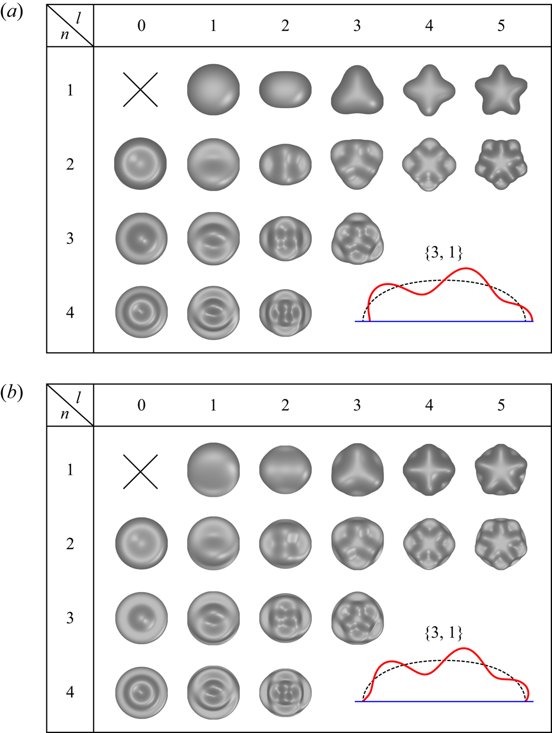
The generalized matrix eigenvalue problems (3.16) and (3.19) for axisymmetric ( $l=0$) and non-axisymmetric ( $l \geq 1$) modes can be solved numerically by using the MATLAB function ‘eig’. Since the sizes of (3.16) and (3.19) are $N$ and $N-1$, respectively, the numbers of corresponding eigenvalues computed are also $N$ and $N-1$, respectively. For a group of solutions with a fixed $l$, the eigenvalues are ordered from small to large, so that the corresponding mode numbers $n$ are sequentially in order from small to large as well. For $l=0$, the first eigenvalue is the dimensionless frequency squared, $\lambda _{2,0}^{2}$, of the mode $\{2,0\}$, while for $l \geq 1$, the first eigenvalue is $\lambda _{1,l}^{2}$ of the mode $\{1,l\}$. The mode number $n$ of the subsequent eigenvalue is the mode number of the present eigenvalue plus one. The vector $\boldsymbol {\phi }_{L}^{*}$ determines the mode shape $y(s)$ defined in (2.13b).
4. Numerical results
In this section the axiBEM model in § 3 is validated by comparing with theoretical and experimental results, and a grid-independence analysis is performed to guarantee the accuracy of the numerical results. Then we systematically investigate the effects of gravity on the axisymmetric and non-axisymmetric oscillations of sessile drops over a wide range of parameters  $\alpha$ and $Bo$, focusing on the frequency shifts of modes due to gravity.
4.1. Verification and convergence
The frequency spectrum of a hemispherical drop with a free CL satisfies the RL spectrum (1.1) with  $k+l$ being even (Lyubimov et al. Reference Lyubimov, Lyubimova and Shklyaev2006). Table 2 shows the comparison between the numerical results of the present model and the theoretical results obtained from (1.1), where the number of free-surface elements is fixed to $N=300$. It is found that numerical and theoretical results are in good agreement and the errors of high modes are larger than those of low modes. For the mode $\{50,5\}$, a relative error $E=| {\lambda /{\lambda _{RL}} - 1} |=0.43\,\%$ can be achieved when $N=300$. It suggests that our model is sufficiently accurate to predict natural frequencies, even for high modes.
Dimensionless frequencies of a hemispherical drop with a free CL calculated by our model ( ${\lambda }$) and by the RL spectrum (1.1) ( ${\lambda _{RL}^{2}}=\omega ^2{\rho {R^3}}/\sigma =(2n+l)(2n+l-2)(2n+l-3)$) and the relative difference $E=| {\lambda /{\lambda _{RL}} - 1} |$ for eight modes $\{n=2, 5, 10,50,l=0, 5\}$. In these cases, the number of free-surface elements is set to $N=300$.

To compare with experimental data, we present the expression of the actual frequency  $f \equiv {\lambda } /({2{\rm \pi} t_*})$ (in Hz) with the characteristic time $t_*$ being defined in (2.9a),
 \begin{equation} f^{2}=\left(\frac{\rho}{\sigma}\right)^{1 / 2}\left(\frac{g}{B o}\right)^{3 / 2}\left(\frac{\lambda}{2 {\rm \pi}}\right)^{2}=\frac{\sigma}{6 {\rm \pi}\rho \tilde{v}} \lambda^{2}. \end{equation}
Expression (4.1) indicates the power law  $f \propto \tilde {v}^{-0.5}$, which is consistent with the experimental observations of Noblin et al. (Reference Noblin, Buguin and Brochard-Wyart2004). This power law only reflects the effects of volume on frequency, ignoring those of gravity on frequency. To verify the cases where gravity plays a significant role ( $Bo \gtrsim 1$), we compare the inviscid prediction of our model with the experiment results of Noblin et al. (Reference Noblin, Buguin and Brochard-Wyart2004) for gravity-flattened drops, as shown in table 3. The excellent agreement of the inviscid predictions with experiments not only validates our model, but also reveals that the inviscid assumption is more appropriate for large drops. This is because the viscous effect of small drops is greater than that of large drops, leading to a larger discrepancy for smaller drops. Furthermore, this discrepancy appears as a systematic overprediction of inviscid results for the 0.1 ml drop, because its viscous effect slightly reduces the natural frequency (Lyubimov et al. Reference Lyubimov, Lyubimova and Shklyaev2006; Chang et al. Reference Chang, Bostwick, Daniel and Steen2015).
Comparison of the natural frequencies (in Hz) between the present model and the experiments of Noblin et al. (Reference Noblin, Buguin and Brochard-Wyart2004) for zonal modes  $\{n,0\}$ of sessile drops with $\alpha =85^{\circ }$ and pinned CLs, where the physical parameters used in (4.1) are $\rho = 998\ {\mathrm {kg}}\ {\textrm {{m}}^{-3}}$, $\sigma = 0.0728 \ {\mathrm { N}} {\mathrm {m}}^{-1}$, $g = 9.81 \ {\mathrm {m}}\ {\mathrm {s}}^{-2}$. Thus, the drop volumes $\tilde {v}=0.1$ ml and $2$ ml correspond to $Bo=1.77$ and 13.04, respectively. In these cases, we set $N=300$.
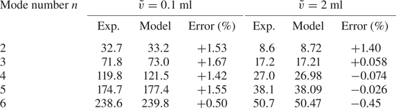
Figure 4(a) shows that the relative error  $E$ decreases with increasing the number of free-surface elements $N$ for three zonal modes of a hemispherical drop with a free CL. This plot is in log-log style for analysing the convergence. The changes of $E$ are well described by power laws (straight lines) with exponents $C\approx 1.8$. This implies that the degree of convergence of our model is roughly second order with respect to the grid density. It is also shown that setting $N$ to 300 can allow for both efficiency and accuracy of the calculation. Therefore, unless otherwise stated, we always set $N=300$ in the following. Figure 4(b) shows that the mode shape $y_{10,0}$ calculated by our model agrees well with that obtained by the RL theory. The inset shows that the model is highly accurate for calculating mode shapes, which can serve as a basis for relevant problems. For example, the problem considering the Hocking condition can be solved by using mode shapes with free CLs as basis functions (Bostwick & Steen Reference Bostwick and Steen2014).
(a) Log-log representation of relative errors  $E=| {\lambda /{\lambda _{RL}} - 1} |$ as a function of the inverse of the grid density, $1/N$, where the frequencies $\lambda$ and $\lambda _{RL}$ are calculated by the present model and the RL theory, respectively. The straight lines are determined by a least square fit, given as $\log (E) = C\log (1/N) + B$. For zonal modes $\{2,0\}$, $\{5,0\}$ and $\{10,0\}$, the slopes of the fitted lines are $C=1.73$, 1.82 and 1.85, respectively. The red solid symbols correspond to the cases of $N=300$. (b) Comparison of mode shape $y_{10,0}$ calculated by our model and by the RL theory. The absolute error is shown in the inset. The maximum of $y(s)$ is scaled to 1 for comparison purposes.

4.2. Frequency shifts due to gravity
Recently, the frequency shifts due to gravity for the axisymmetric modes of sessile drops have been investigated by a direct numerical simulation based on the Navier–Stokes equations (Sakakeeny & Ling Reference Sakakeeny and Ling2020, Reference Sakakeeny and Ling2021). It was found that the frequencies of the first few axisymmetric modes increase (decrease) with increasing the Bond number (contact angle). However, the question of how gravity affects the frequencies of other modes has not been answered, especially for non-axisymmetric modes. The simulation of non-axisymmetric oscillations requires a large amount of computing resources (three-dimensional numerical simulation). Since our model is based on the normal-mode framework (§ 2.3), the model can efficiently and accurately predict the frequencies of both the axisymmetric ( $l=0$) and non-axisymmetric ( $l\geq 1$) modes. We study the frequency shifts for contact angles $\alpha \in [30^{\circ },150^{\circ }]$ and Bond numbers $Bo \in [0,10]$. Note that the drop volume is kept constant at $v=2{\rm \pi} /3$ to exclude the volume effects on frequency (as reflected in the relation (4.1)).
To measure the frequency shifts due to gravity, we define a shift factor  $S_{n,l}$ for mode $\{n,l\}$,
 \begin{equation} S_{n,l}(\alpha,Bo)=\frac{\lambda_{n,l}(\alpha,Bo)}{\lambda _{n,l}^*(\alpha)}-1, \end{equation}
where  $S_{n,l}$ and $\lambda _{n,l}$ are functions of $\alpha$ and $Bo$, and $\lambda _{n,l}^*=\lambda _{n,l}(\alpha,0)$ is the frequency in the absence of gravity. The value of $S_{n,l}$ denotes the relative change of frequency and $S_{n,l}>0$ ( ${<}0$) represents an upward (downward) shift of frequency for given values of $\alpha$ and $Bo$.
$Bo$.
4.2.1. Zonal modes  $\{n>1,l=0\}$

For  $Bo=0$, we reproduce the plots of the frequency $\lambda _{n,0}^*$ versus the contact angle $\alpha$ by using the present model and the self-coded Bostwick and Steen (BS) model (which is self-programmed with an in-house MATLAB code by following Bostwick & Steen Reference Bostwick and Steen2014), as shown in figure 5. Note that in the code of the self-coded BS model, the boundary parameter $\chi$ for the free CL condition (2.14e) is $\chi =-\cos (\alpha )$ rather than $\chi =\cos (\alpha )$ as adopted by Bostwick & Steen (Reference Bostwick and Steen2014), where the reason can be found in § 5.1. The results show an excellent agreement between our model and the self-coded BS model, except for the high modes $\{5,0\}$ and $\{6,0\}$, where there are small discrepancies at large contact angles. These discrepancies can be reduced by increasing the number of basis functions for the self-coded BS model. However, the results of high modes with small contact angles reported in Bostwick & Steen (Reference Bostwick and Steen2014) differ significantly from those calculated by our model and the self-coded BS model. For example, for the mode $\{6,0\}$ with a pinned CL and $\alpha =42.4^{\circ }$, the self-coded BS model predicts the dimensionless frequency $\lambda _{6,0}^*=33.87$ while the data of Bostwick & Steen (Reference Bostwick and Steen2014) is 41.34 (see figure 5b). Obviously, the former agrees reasonably with the experimental result of 32.88 (Chang et al. Reference Chang, Bostwick, Daniel and Steen2015) and the prediction of 34.81 by the toroidal model (Sharma & Wilson Reference Sharma and Wilson2021). The comparison demonstrates that the self-coded BS model developed by Bostwick & Steen (Reference Bostwick and Steen2014) can accurately predict the frequencies of high modes with small contact angles. Our model recovers the results of zonal modes for the spherical-cap drop with free and pinned CLs.
Frequency spectrum of zonal ( $l=0$) modes in the absence of gravity ( $Bo=0$) for the (a) free and (b) pinned CL conditions. Frequencies of the first five modes ( $n=2, 3, 4, 5, 6$) are calculated by the present model and by the self-coded BS model. In (b) the frequency of the mode $\{6,0\}$ with $\alpha =42.4^{\circ }$ is compared with the experiment result of Chang et al. (Reference Chang, Bostwick, Daniel and Steen2015) and the theoretical results of Bostwick & Steen (Reference Bostwick and Steen2014) and Sharma & Wilson (Reference Sharma and Wilson2021).

Figure 6 shows how the frequencies of zonal modes are affected by gravity. There are three different trends for the shift factor  $S_{n,0}$ over $Bo$ with a fixed contact angle.
(i) For the mode
$\{2,0\}$ with $\alpha =45^{\circ }$, the shift factor $S_{2,0}$ increases initially and then decreases as $Bo$ increases (figure 6a). A similar trend is also observed for the mode $\{6,0\}$ with $\alpha =90^{\circ }$ (figure 6b). The difference is that, when $Bo\gtrsim 2$, the former has a shift factor $S_{2,0}(45^{\circ },Bo)$ that is less than zero, while the latter always has a shift factor greater than zero. This means that there is a critical value (${\approx }2$) of $Bo$ that keeps the frequency of the mode $\{2,0\}$ with $\alpha =45^{\circ }$ unchanged (i.e. $S_{2,0}=0$), and gravity shifts the frequency downwards when $Bo \gtrsim 2$.(ii) For the higher modes
$n>2$ with $\alpha =45^{\circ }$ (figure 6a), $S_{n,0}$ decreases monotonically with the increase of $Bo$.(iii) For other modes with larger contact angles (figure 6b,c), the frequency increases as
$Bo$ increases, which is consistent with the observations of Sakakeeny & Ling (Reference Sakakeeny and Ling2020, Reference Sakakeeny and Ling2021).


The first two trends show that the gravity can shift the frequency downwards for sessile drops with small contact angles. For example, for a water drop ( $\rho = 998\ {\mathrm {kg}}\ {{\mathrm {m}}^{-3}}$, $\sigma = 0.0728 \ {\mathrm {N}}\ {\mathrm {m}}^{-1}$) with volume $\tilde v=1.343\ \mathrm {ml}$, contact angle $\alpha =45^{\circ }$ and pinned CL, the frequencies of the first two modes $\{2,0\}$ and $\{3,0\}$ are reduced respectively by about $7\,\%$ and $15\,\%$ in the Earth's gravitational field $g= 9.81 \ {\mathrm {m}}\ {\mathrm {s}}^{-2}$ ( $Bo=10.0$) compared with in a microgravity environment ( $Bo \rightarrow 0$), as shown in supplementary movie 1 available at https://doi.org/10.1017/jfm.2023.252.
Effects of gravity on frequency for zonal modes: (a–c) the shift factor  $S_{n,0}$ versus the Bond number $Bo$ for fixed contact angles (a) $\alpha =45^{\circ }$, (b) $90^{\circ }$ and (c) $135^{\circ }$ and (d) $S_{n,0}$ vs $\alpha$ for fixed Bond number $Bo=1.389$. Results are shown for the first five modes ( $n=2,3,4,5,6$) with free (black solid) and pinned (blue dashed) CLs. In (d) results of direct numerical simulations by Sakakeeny & Ling (Reference Sakakeeny and Ling2021) for the mode $\{2,0\}$ with a pinned CL are denoted by $\bigcirc$ and a good agreement is observed, where the corresponding Bond number in Sakakeeny & Ling (Reference Sakakeeny and Ling2021) is 0.88 due to the use of different scalings.

To the best of our knowledge, for zonal modes, the downward frequency shift due to gravity has not been observed in previous literature. This may be because the frequency decrease with increasing gravity only occurs at small contact angles and the magnitude of the decrease is much smaller relative to the increase (figure 6d). For example, in the parameter domain ( $Bo \in [0,1.389]$ and $\alpha \in [50^{\circ },150^{\circ }]$) adopted by Sakakeeny & Ling (Reference Sakakeeny and Ling2020, Reference Sakakeeny and Ling2021) the frequency is always shifted upwards by gravity. Their simulation results agree well with our inviscid predictions, e.g. for zonal modes $\{2,0\}$ with pinned CLs and $Bo=1.389$ (see figure 6d).
From figure 6, we see that the modes with free CLs are more susceptible to gravity than those with pinned CLs, especially for the lower modes. That is, the mode with a free CL has a larger frequency shift than the mode with a pinned CL and their difference decreases with increasing the mode number  $n$. It is further observed from figure 6(d) that the zonal modes with a larger contact angle are more sensitive to the effects of gravity, consistent with the observations of Sakakeeny & Ling (Reference Sakakeeny and Ling2020, Reference Sakakeeny and Ling2021).
4.2.2. Sectoral modes $\{n=1,l\geq 1\}$

The sectoral modes  $\{1,l\}$ are star shaped, which have one layer with $l$ sectors (see figure 3). Figure 7 plots the frequencies of sectoral modes against contact angle $\alpha$ for $Bo=0$ and $Bo=5$. In the presence of gravity, most of the sectoral modes show a significant decrease in frequency at all contact angles. This differs from previous findings for the zonal modes. For example, for a drop with $\alpha =90^{\circ }$ and a free CL, the frequency of the zonal mode $\{2,0\}$ increases at $Bo=5$ by $S_{2,0}(90^{\circ },5)=43.31\,\%$, while the sectoral mode $\{1,10\}$ appears to decrease in frequency by $|23.44/32.87-1|\approx 28.69\,\%$ at the same Bond number (see supplementary movie 2). It follows that, for different modes, the frequency shifts due to gravity are different or even opposite.
Frequency spectrum of sectoral  $\{n=1,l\geq 1\}$ modes with $Bo=0$ and $Bo=5$, for the (a) free and (b) pinned CL conditions. From bottom to top the corresponding azimuthal wavenumbers of spectral lines are $l=1,2,3,4,5,10$.

It is noteworthy that the numerical results for the frequency of the Noether mode  $\{1,1\}$ with a free CL are all zero regardless of $\alpha$ with or without gravity (see the solid and dashed bottom lines in figure 7a). The observation of $\lambda _{1,1}=0$ is related to the walking drop instability. Details will be discussed in § 5.1.
Figure 8 shows the frequency shifts for sectoral modes with fixed contact angles ( $\alpha =45^{\circ },90^{\circ },135^{\circ }$). For free CLs, the frequencies decrease with increasing $Bo$ for all three contact angles, and the higher the azimuthal wavenumber $l$, the smaller the relative frequency decrease (figure 8a–c). The downward frequency shifts for pinned CLs are smaller than for free CLs, and upward frequency shifts even occur for the modes $\{1,1\}$ with pinned CLs and large contact angles (figure 8d–f). Moreover, the dependence of the relative frequency decrease on $l$ for pinned CLs is opposite to that for free CLs (see the directions of arrows). Similar to zonal modes, the sectoral modes with free CLs are also more susceptible to gravity than those with pinned CLs. However, the frequency shifts for sectoral modes are not sensitive to the change of contact angle (with the exception of the mode $\{1,1\}$ with a pinned CL whose frequency shift is strongly influenced by contact angle).
Effects of gravity on frequency for sectoral modes:  $S_{1,l}$ vs $Bo$ for fixed contact angles (a,d) $\alpha =45^{\circ }$, (b,e) $90^{\circ }$ and (c,f) $135^{\circ }$ with the (a–c) free and (d–f) pinned CL conditions.

4.2.3. Tesseral modes $\{n>1,l\geq 1\}$

Figure 9 compares the frequency spectra of three groups ( $l=1,5,10$) of tesseral modes with $Bo=0$ and $Bo=5$. For $Bo=0$, the spectrum of $l=1$ has a similar pattern to that of the zonal modes (see figure 5), in the sense that both have low frequencies at small and large contact angles and high frequencies at intermediate contact angles ( ${\approx }70^{\circ }$). For larger $l$, the frequencies of low modes at large contact angles becomes higher compared with small contact angles. Under gravity, the frequencies of most tesseral modes decrease at small contact angles and increase at large contact angles, similar to zonal modes. However, some modes with small $n$ and large $l$ (e.g. the modes $\{1,5\}$ and $\{3,10\}$ with free CLs) show a decrease in frequency at all contact angles, similar to sectoral modes.
Frequency spectrum of tesseral  $\{n>1,l\geq 1\}$ modes with $Bo=0$ and $Bo=5$, for the (a–c) free and (d–f) pinned CL conditions. The results are grouped according to the azimuthal wavenumber $l$ and are presented separately for $l=1,5,10$. In each group, the layer numbers of spectral lines from bottom to top are $n=2,3,4,5,6$.

We observe that the frequencies of tesseral modes are always shifted downward at small contact angles. The main difference among these modes is how gravity affects frequency at intermediate and large contact angles. Figure 10 plots the shift factor  $S_{n,l}$ vs $Bo$ for $\alpha =90^{\circ }$. For $l=1,2,3$, the frequencies of the first five tesseral modes are always shifted upwards. For $l=1$, the relative frequency change of the mode with smaller $n$ is larger. For $l=2,3$, however, the dependence of the relative frequency change on the mode number $n$ is progressively reversed as $l$ increases (see the directions of arrows in figure 10b,c). For $l>3$, the frequencies of modes with small $n$ are shifted downwards at $\alpha =90^{\circ }$. In general, the frequency shifts due to gravity for tesseral modes with large $n$ and small $l$ are similar to those for zonal modes, while modes with small $n$ and large $l$ are similar to sectoral modes.
Effects of gravity on frequency for tesseral modes with fixed contact angle  $\alpha =90^{\circ }$: $S_{n,l}$ vs $Bo$ for $l=1,2,3,4,5,10$. For each azimuthal wavenumber $l$, results are shown for the first five modes ( $n=2,3,4,5,6$) with free and pinned CLs.

4.2.4. Phase diagram
We study the frequency shifts for contact angles  $\alpha \in [30^{\circ },150^{\circ }]$ and Bond numbers $Bo \in [0,10]$. For zonal modes, we observe downward and upward frequency shifts at small and large contact angles, respectively. This feature can be illustrated by a typical contour (type I) of the shift factor $S_{n,l}$, as shown in figure 11(a). It is shown that, whether the frequency of mode $\{2,0\}$ with a free CL increases or decreases depends on the position of the phase point $(\alpha,Bo)$: when $(\alpha,Bo)$ is in the blue region to the left side of the contour $S_{2,0}=0$, the frequency is shifted downwards, whereas the opposite occurs when $(\alpha,Bo)$ is in the red region. However, most sectoral modes exhibit a downward frequency shift at all contact angles, as reflected by the second typical contour (type II) of $S_{n,l}$ (figure 11b). These shift factors $S_{n,l}$ are always less than zero regardless of $\alpha$ and $Bo$. For tesseral modes, both the typical contours of $S_{n,l}$ can occur, depending on the mode number pair $\{n,l\}$.
Two typical contours of the shift factor  $S_{n,l}$: (a) type I, a region of $S_{n,l}<0$ (blue) on the left and a region of $S_{n,l}>0$ (red) on the right, separated by a critical contour line of $S_{n,l}=0$ for mode $\{2,0\}$ with a free CL; and (b) type II, a complete region of $S_{n,l}<0$ for mode $\{1,2\}$ with a free CL. Here and in what follows, all contours are generated from $100\times 100$ uniformly distributed cases in the region $\alpha \in [30^{\circ }, 150^{\circ }]\times Bo\in [0, 10]$.

In addition to the two typical contours (types I and II), contours with other shapes are collectively referred to as transitional contours (type T), because these contours are transitions between types I and II. Figure 12 shows four common shapes of type T. We note that the classification of the contours depends on the ranges of  $\alpha$ and $Bo$. For example, reducing the upper limit of the range of $\alpha$ from $150^{\circ }$ to $130^{\circ }$, the contour of the mode $\{2,3\}$ with a free CL (figure 12b) will be classified as type I. This means that the ranges of parameters we have chosen still cannot capture all the features of contours for some modes. On the other hand, the ranges of parameters in this work are reasonable because they cover the vast majority of real physical situations.
Four common shapes of transitional contours of  $S_{n,l}$ (type T) for (a) mode $\{1,2\}$ with a pinned CL, (b) mode $\{2,3\}$ with a free CL, (c) mode $\{3,6\}$ with a free CL and (d) mode $\{4,10\}$ with a pinned CL, respectively. The transitional contours are transitions between types I and II.

We classify the contours of  $S_{n,l}$ for modes with $l=0$ to 10 and $n=1$ to 10 as types I, II and T, as shown in figure 13. Results are given for both the free and pinned CL conditions. For zonal modes, all contours are of type I. For sectoral modes, except for the modes $\{1,1\}$ and $\{1,2\}$ with a pinned CL and the mode $\{1,1\}$ with a free CL, the contours are of type II. For tesseral modes, all the three types (I, II and T) of contours are possible, where the mode with larger $n$ (
$n$ ( $l$) is more likely of type I (II) and the remaining modes in the middle are categorized as type T. It follows that the frequencies of sectoral modes tend to be shifted downwards at large contact angles, whereas the zonal modes ( $l=0$) exhibit upward frequency shifts under the same conditions. Note that the contour cannot be given and classified for the mode $\{1,1\}$ with a free CL because its frequency is constant at zero regardless of $\alpha$ and $Bo$.
$Bo$.
Types of contours of  $S_{n,l}$ for modes with (a) free and (b) pinned CLs, where $n=1,2,\ldots,10$ and $l=0,1,\ldots,10$.

The modes  $l=1$ are called ‘rocking modes’ because their one sector rocks side to side during the vibration. It is seen from figure 13 that the contours of $S_{n,l}$ for both zonal ( $l=0$) and rocking ( $l=1$) modes are of type I. Thus, there is a critical contour line $S_{n,l}=0$ for each mode: when the phase point $(\alpha,Bo)$ crosses the critical line, the shift factor $S_{n,l}$ changes its sign, and there is a downward frequency shift on the left side of the critical line and an upward shift on the right side (see figure 11a). Figure 14 shows the critical lines for the first five zonal modes and the first five rocking modes, respectively. Results for modes with free and pinned CLs are shown paired, and their differences are not significant. As $n$ increases, the critical line shifts to the right, but even for higher modes $\{6,0\}$ and $\{5,1\}$ the critical lines are still in the region of $\alpha <90^{\circ }$. Therefore, the frequencies of the low zonal and rocking modes for $\alpha \geq 90^{\circ }$ are always shifted upwards by gravity. Moreover, except for the mode $\{1,1\}$ with a free CL, gravity always shifts the frequency downwards as long as the contact angle is small enough ( $\alpha \lesssim 40^{\circ }$).
Phase diagram  $\alpha$– $Bo$ of the frequency shifts for (a) zonal ( $l=0$) modes and (b) rocking ( $l=1$) modes. For a given mode, when the point $(\alpha,Bo)$ lies to the left (right) of the critical line $S_{n,l}=0$, the frequency of that mode is shifted downwards (upwards) by gravity.

5. Discussion of results
Here we discuss some interesting consequences resulting from the frequency shifts under the influence of gravity, including whether the walking drop instability (Bostwick & Steen Reference Bostwick and Steen2014) exists, how gravity breaks the spectral degeneracy of the free semi-drop and the determination of the lowest mode.
5.1. Noether mode $\{1,1\}$: walking drop instability

Walking drop instability, similar to the Rayleigh–Plateau instability, is a capillary instability whose interface is reshaped according to its instability mode (Bostwick & Steen Reference Bostwick and Steen2014, Reference Bostwick and Steen2015). As the name suggests, this instability behaves as a spontaneous horizontal movement of spherical-cap drops with free CLs and contact angle  $\alpha >90^{\circ }$ on a plane, where the horizontal motion corresponds to the mode $\{1,1\}$. Because the mode $\{1,1\}$ of a spherical drop has zero frequency according to Noether's theorem, this mode is referred to as the Noether mode by Bostwick & Steen (Reference Bostwick and Steen2014). The walking drop instability is inferred from the finding of Bostwick & Steen (Reference Bostwick and Steen2014) that the frequency of the Noether mode $\{1,1\}$ with a free CL satisfies $\lambda _{1,1}^{2}<0$ for $\alpha >90^{\circ }$ and $Bo=0$. However, a wrong free CL condition has been used in the work of Bostwick & Steen (Reference Bostwick and Steen2014), which leads to an incorrect calculation of $\lambda _{1,1}^{2}$. More specifically, their omission of the minus sign for the curvature $k_{1}=-\sin \alpha$ of spherical-cap drops results in the missing of the minus sign in the boundary parameter $\chi =-\cos \alpha$. The discussion about the sign of the principal curvature $k_1$ can be found in Appendix A.
5.1.1. Reproducing the walking drop instability with the wrong condition
To demonstrate the above, we adopt the wrong CL condition (i.e.  $k_1=\sin \alpha$) to reproduce the results of Bostwick & Steen (Reference Bostwick and Steen2014) by using the axiBEM model and the self-coded BS model, as shown in figure 15. The results of the self-coded BS model are generated by using a self-programmed code following Bostwick & Steen (Reference Bostwick and Steen2014), while the results of Bostwick & Steen (Reference Bostwick and Steen2014) are those reported in their paper. It is shown that the results of the wrong CL condition qualitatively agree with those of Bostwick & Steen (Reference Bostwick and Steen2014), that is, $\lambda _{1,1}^{2}> 0$ for $\alpha < 90^\circ$ and $\lambda _{1,1}^{2}<0$ for $\alpha >90^\circ$, resulting in the walking instability of hydrophobic drops with free CLs. Furthermore, the results of the axiBEM and self-coded BS models agree very well when using the wrong CL condition. However, these results quantitatively differ significantly from those reported by Bostwick & Steen (Reference Bostwick and Steen2014). For instance, our result shows the maximum instability growth is $\lambda ^{2}=-0.6994$ at $\alpha =117.4^\circ$, while the result of Bostwick & Steen (Reference Bostwick and Steen2014) is the maximum $\lambda ^{2}=-0.0458$ at $\alpha =132.5^\circ$. In view of the above, we believe that the above discrepancies might be due to other obscure reasons.
Numerical results of  $-\lambda _{1,1}^{2}$ against $\alpha$ with $Bo=0$ for the wrong free CL condition. For comparison, the results for the correct CL condition (dash-dotted line) are drawn. In these cases, the scaling is the same as in Bostwick & Steen (Reference Bostwick and Steen2014), and the grid number of the axiBEM model is set to $N=300$.

When we adopt the correct form of the free CL condition (2.18), we find a power law
 \begin{equation} \lambda_{1,1}^{2} \propto N^{{-}1.90} \end{equation}
for the numerical results of  $\alpha =135^{\circ }$ and $Bo=5$ by using our model, as shown in figure 16. This implies that the numerical result of ${\lambda _{1,1}^{2}}$ decays to zero as the grid density $N \to \infty$. Since the numerical results cannot precisely reach zero frequency, we can infer from (5.1) that
 \begin{equation} {\lambda _{1,1}}(\alpha,Bo) = 0 \end{equation}
always holds regardless of  $\alpha$ and $Bo$ (see also figure 7a). Equation (5.2) implies that the translational invariance related to the Noether mode $\{1,1\}$ with a free CL is not broken by varying the contact angle $\alpha$ or the Bond number $Bo$, which is also consistent with the expectation from static stability theory (see § 5.1.3).
Numerical results for the frequency squared  $\lambda _{1,1}^{2}$ of the Noether mode $\{1,1\}$ with a free CL as a function of $1/N$, where $\alpha =135^{\circ }$ and $Bo=5$. The inset shows the base state (dashed line) and the mode shape (solid line).

5.1.2. Effect of the wrong free CL condition on other modes
Apparently, the principal curvature of the surface is not included in the pinned CL condition (2.19), so the pinned results are not affected by the wrong CL condition. However, even when the same CL conditions are adopted, there are still some discrepancies between our calculations and the results reported in Bostwick & Steen (Reference Bostwick and Steen2014), as shown in the previous section. To further analyse the discrepancies, we reproduce the pinned results of  $Bo=0$ to compare with the experimental and theoretical results reported in Chang et al. (Reference Chang, Bostwick, Daniel and Steen2015), as shown in figure 17. It is shown that, in general, our results are in better agreement with the experimental results, especially for high modes with small contact angles. Moreover, we have shown that the results of the self-coded BS model following Bostwick & Steen (Reference Bostwick and Steen2014) agree very well with those of the axiBEM model (figures 5). Thus, the discrepancies should be due to some other obscure reasons. Since the discrepancy is only significant for high modes with small $\alpha$, the validation of Bostwick & Steen (Reference Bostwick and Steen2014) still holds.
Frequency comparisons of our results with those of Chang et al. (Reference Chang, Bostwick, Daniel and Steen2015) for (a) zonal modes, (b) sectoral modes, (c)  $n=2$ tesseral modes and (d) $n=3$ tesseral mode. The solid and dashed lines indicate the results of the axiBEM model and those of the inviscid theory (Bostwick & Steen Reference Bostwick and Steen2014) reported in Chang et al. (Reference Chang, Bostwick, Daniel and Steen2015), respectively, and the symbols indicate their experimental results. Here the scaling is the same as in Bostwick & Steen (Reference Bostwick and Steen2014).

Figure 18 shows the effect of the wrong condition on the modes with free CLs. We observe the frequency ratio  $\lambda _w/\lambda >1$ for $\alpha <90^\circ$ and $\lambda _w/\lambda <1$ for $\alpha >90^\circ$, where $\lambda _w$ is obtained from the wrong condition. This implies that the wrong condition causes frequencies for small contact angles to be overestimated and frequencies for large contact angles to be underestimated, and therefore, is independent of modes with $\alpha =90^{\circ }$ (since the wrong condition becomes consistent with the correct one in this case). We also observe that the wrong condition is insensitive to high modes and only has a limited effect on a few low modes with contact angles away from $90^\circ$. Thus, even with the wrong condition, the verification and most of the conclusions of Bostwick & Steen (Reference Bostwick and Steen2014) are still valid.
Frequency ratios  $\lambda _w/\lambda$ due to the wrong CL condition for modes with (a) $l=0$, (b) $l=1$, (c) $l=5$ and (d) $l=10$, where the subscript $w$ indicates the wrong condition. The layer numbers of modes are (a,b) $n=2$, 3, 4, 5, 10 and (c,d) $n=1$, 2, 3, 4, 10 along the arrow.

5.1.3. Demonstration through static stability theory
To further justify (5.2), we relate this dynamic problem to the theory of static stability (Bostwick & Steen Reference Bostwick and Steen2015). For the considered configuration, the static stability problem is given by (Myshkis et al. Reference Myshkis, Babskii, Kopachevskii, Slobozhanin and Tyuptsov1987, p. 129)
 \begin{equation} -{\psi _1^{\prime \prime }} - \frac{{r'}}{r}{\psi _1^\prime } + \left[ {Bo\times r' - \left( {{k_1}^2 + {k_2}^2} \right) + \frac{{{1}}}{{{r^2}}}} \right]\psi _1 = \lambda_1^s\psi _1, \end{equation}
with the boundary condition
 \begin{equation} \psi _1^\prime(s_c)+\chi \psi _1(s_c)=0, \end{equation}
where  $\psi _1$ and $\lambda _1^s$ denote eigenfunctions and eigenvalues, respectively.
From a mathematical point of view, when  $\lambda _{1,1} = 0$, the dynamic problem (2.14) has the same form as the static stability problem (5.3) with a zero eigenvalue $\lambda _1^s=0$ corresponding to the mode $\{1,1\}$. In this case, the static and dynamic problems have the same solutions (i.e. eigenfunctions and eigenvalues). This means that when the eigenvalue of the static stability problem is zero, the eigenvalue of the dynamic problem of the corresponding mode is also zero. In other words, the static stability can be recovered from the dynamic stability, and the thresholds for the two instabilities are essentially the same. Only if the boundary parameter $\chi$ is equal to the critical boundary parameter $\chi _{1,1}^{*}$, the corresponding eigenvalue of the static stability problem is zero (Myshkis et al. Reference Myshkis, Babskii, Kopachevskii, Slobozhanin and Tyuptsov1987; Bostwick & Steen Reference Bostwick and Steen2015). The critical boundary parameter is (Myshkis et al. Reference Myshkis, Babskii, Kopachevskii, Slobozhanin and Tyuptsov1987, p. 141)
 \begin{equation} \chi_{1,1}^{*}={-}{{k_1(s_c)} \frac{r'(s_c)}{z'(s_c)} } ={{k_1(s_c)}\cot \alpha }. \end{equation}
Comparing (2.16) and (5.5), it is easy to see that  $\chi =\chi _{1,1}^{*}$ for the free CL condition. Hence, the dynamic and static stability problems both have zero eigenvalue (frequency) corresponding to the Noether mode with a free CL. It suggests that the frequency of the mode $\{1,1\}$ of sessile drops with free CLs on a plane is always zero regardless of $\alpha$ and $Bo$.
$Bo$.
In summary, we verify numerically and mathematically that  ${\lambda _{1,1}} = 0$ regardless of $\alpha$ and $Bo$, and therefore, demonstrate that there is no walking drop instability related to the Noether mode $\{1,1\}$ for sessile drops with free CLs and $\alpha >90^{\circ }$ regardless of the presence of gravity. This finding contradicts with the conclusions of Bostwick & Steen (Reference Bostwick and Steen2014), owing to the wrong form of the free CL condition used in the latter.
5.2. Breaking of spectral degeneracy
For a hemispherical drop ( $\alpha =90^{\circ }$ and $Bo=0$) with a free CL (i.e. the free semi-drop), all the modes with the same polar wavenumber $k=2n-2+l$ have the same frequency, which is known as the spectral degeneracy with respect to the azimuthal wavenumber $l$ (Bostwick & Steen Reference Bostwick and Steen2015). This degeneracy is inherited from the free drop problem (refer to (1.1)), and can be represented mathematically by
 \begin{equation} {\lambda _{n,l}}(90^{{\circ}},0) = {\lambda _{n - 1,l + 2}}(90^{{\circ}},0). \end{equation}
For a given  $k$, there are a total of $\lfloor k/2 \rfloor +1$ modes with the same frequency given by the RL spectrum (1.1) in dimensionless form ( $\lambda =\omega \sqrt {{\rho {R^3}}/\sigma }$), where $\lfloor\ \rfloor$ denotes the rounding down operation. Prior studies (e.g. Lyubimov et al. Reference Lyubimov, Lyubimova and Shklyaev2006; Bostwick & Steen Reference Bostwick and Steen2014) have found that the spectral degeneracy can be broken by the contact angle or the mobility parameter that characterizes the mobility of the CL (see § 1).
We find that this degeneracy can also be broken by gravity. Figure 19 shows the frequencies of modes with free CLs and  $\alpha =90^{\circ }$ as a function of $Bo$ for fixed polar wavenumbers ( $k=2, 3, 4, 5$). For $Bo=0$, the modes with the same $k$ have the same frequency, reflecting the spectral degeneracy just described. As $Bo$ increases, the splitting of frequencies occurs in a way that leads to lower frequencies for a higher azimuthal wavenumber $l$. Consequently, the spectral degeneracy described by (5.6) is broken by gravity.
Breaking of the spectral degeneracy for modes with free CLs and  $\alpha =90^{\circ }$: frequency $\lambda _{n,l}$ versus the Bond number $Bo$ for fixed polar wavenumber (a) $k=2$, (b) $k=3$, (c) $k=4$ and (d) $k=5$, where the layer number $n$ is determined by (3.20). The dots indicate the spectral degeneracy at $Bo=0$ (see also figure 2 in Bostwick & Steen Reference Bostwick and Steen2014), where the frequency is given by $\lambda ^2=k(k-1)(k+2)$.

5.3. Lowest mode
The lowest mode is that with the lowest non-zero frequency of all modes, which is generally the dominant mode and is more likely to be excited. For free CLs, the lowest mode of a sessile drop with  $\alpha >90^{\circ }$ in the absence of gravity (i.e. $Bo=0$) is the zonal mode $\{2,0\}$, while the lowest mode of a drop with $\alpha <90^{\circ }$ is the sectoral mode $\{1,2\}$, as shown in figure 20(a). As $Bo$ increases, the lowest mode of a drop with $\alpha >90^{\circ }$ gradually changes from mode $\{2,0\}$ to $\{1,2\}$ (figure 20b). This is because, for $\alpha >90^{\circ }$, the frequencies of sectoral modes decrease under gravity, while the frequencies of zonal modes increase. As a result, the lowest mode becomes the sectoral mode $\{1,2\}$ at $Bo=2$ (figure 20c). Note that the mode $\{1,1\}$ with a free CL cannot be the lowest mode due to its zero frequency (§ 5.1). However, for pinned CLs, the mode $\{1,1\}$ that has a non-zero frequency is always the lowest mode, even if its frequency increases significantly under gravity at large contact angles (see figure 8f).
The lowest mode with a free CL for  $Bo=0,1,2$. In (a) the lowest mode in the absence of gravity is $\{1,2\}$ for $\alpha <90^{\circ }$ and $\{2,0\}$ for $\alpha >90^{\circ }$. In (b,c) the lowest mode (red line) gradually changes from $\{2,0\}$ to $\{1,2\}$ for $\alpha >90^{\circ }$.

In experiments, the CL in the non-axisymmetric oscillations of large drops ( $Bo \gg 1$) is usually movable (see e.g. Noblin et al. Reference Noblin, Buguin and Brochard-Wyart2004). Therefore, from the above conclusions we can see that, for large drops, the lowest mode is usually the non-axisymmetric mode $\{1,2\}$, which means that large drops may be more prone to non-axisymmetric oscillations than small drops.
6. Summary and conclusions
We have investigated the natural oscillations of sessile drops on a plane under gravity. In the linear inviscid limit, the oscillation problem is reduced to the functional eigenvalue problem (2.14) by the normal-mode decomposition. Due to the limitations of theoretical models on the drop shape, we have developed an axiBEM model to numerically solve (2.14), in which both the free and pinned CL conditions are considered. It should be noted that even though our model uses the axiBEM formulation, non-axisymmetric oscillations can be considered through the normal-mode decomposition (2.13). The model is independent of the drop geometry and can be easily extended to drops of arbitrary shape. It has been validated against analytical results, and was shown to achieve the second-order convergence with mesh refinement. The excellent agreement of the inviscid predictions with the experiments of Noblin et al. (Reference Noblin, Buguin and Brochard-Wyart2004) in a terrestrial gravity environment further confirms the accuracy of our model.
There have been various axiBEM models developed to determine the vibrational characteristics of axisymmetric liquid surfaces (Siekmann & Schilling Reference Siekmann and Schilling1989; Ebrahimian et al. Reference Ebrahimian, Noorian and Haddadpour2013, Reference Ebrahimian, Noorian and Haddadpour2015, and references given therein). Most of these axiBEM models are designed for modal analysis of liquid sloshing inside a vessel and, therefore, usually consider flat liquid surfaces. Compared with Siekmann & Schilling (Reference Siekmann and Schilling1989) using the indirect formulation of axiBEM, our model uses the more intuitive direct formulation in Ebrahimian et al. (Reference Ebrahimian, Noorian and Haddadpour2013, Reference Ebrahimian, Noorian and Haddadpour2015) for the purpose of one-dimensional reduction. To extend to drops with curved surfaces, the free-surface governing equation together with the Young–Laplace equation in our model is solved in curvilinear coordinates and the free CL condition for non- $90^\circ$ contact angles is considered. Besides, the volume constraint is included in our model to eliminate the non-physical volume mode $\{1, 0\}$. Compared with the axiBEM models of liquid sloshing, our model allows for curved liquid surfaces.
In the presence of gravity, not only does the drop flatten, but an additional restoring force is introduced for the oscillations, resulting in the frequency shifts of modes. It was found that the effects of gravity on frequency are different or even opposite for different modes. Overall, there are three types of  $\alpha$– $Bo$ diagrams reflecting how gravity shifts the frequency. For the zonal modes, gravity shifts the frequency downwards at small contact angles, and upwards when the contact angle exceeds a certain critical value. That is, there is a longitudinally inclined critical line in the $\alpha$– $Bo$ diagram (type I, figure 11a). For most sectoral modes, gravity always shifts the frequency downwards regardless of $\alpha$ and $Bo$ (type II, figure 11b). For the tesseral modes, both types I and II can occur, depending on the mode number pair $\{n,l\}$. Generally, type I is more likely to occur for modes with small $l$ and large $n$ and type II is for large $l$ and small $n$, with more complex frequency shift diagrams (type T, figure 12) possible in between (see figure 13). Interestingly, except for the Noether mode $\{1,1\}$ with a free CL, gravity always shifts the frequency downwards as long as the contact angle is small enough. The counter-intuitive behaviour of the frequency spectrum suggests that the effects of gravity on the oscillations of drops with small contact angles differ dramatically from those with large contact angles.
The frequency shifts of the modes due to gravity can lead to some interesting results. For example, gravity can break the spectral degeneracy of the free semi-drop. This breaking follows that ‘the larger the  $l$, the lower the frequency’ (figure 19), in contrast to the spectral breaking by the CL pinning (Lyubimov et al. Reference Lyubimov, Lyubimova and Shklyaev2006). Similarly, gravity can change the lowest mode of a drop with a free CL and $\alpha >90^{\circ }$ gradually from mode $\{2,0\}$ to $\{1,2\}$ (see figure 20). The Noether mode $\{1,1\}$ with a free CL is the only mode whose frequency is not shifted by gravity and is always zero regardless of $\alpha$ and $Bo$. This finding is verified numerically by our model and mathematically by the static stability theory. In other words, our results suggest that the walking drop instability reported by Bostwick & Steen (Reference Bostwick and Steen2014) does not exist.
Supplementary movies
Supplementary movies are available at https://doi.org/10.1017/jfm.2023.252.
Funding
We are grateful for the support of the National Natural Science Foundation of China (grant numbers 12102426, 11425210, 11621202, 11672288, 11932019), the China Postdoctoral Science Foundation (grant number 2021M693080), the Strategic Priority Research Program of the Chinese Academy of Sciences (grant number XDB22040103) and the Fundamental Research Funds for the Central Universities.
Declaration of interests
The authors report no conflict of interest.
Appendix A. On the sign of the principal curvatures of $\varGamma$

For an axisymmetric drop surface (figure 21), the sign of its principal curvatures can be arbitrary and depends only on the direction of the unit normal vector  $\boldsymbol {N}$. The mean curvature is related to the unit normal by (see Weatherburn Reference Weatherburn1955, p. 225)
 \begin{equation} 2H={-}\boldsymbol{\nabla}\boldsymbol{\cdot}\boldsymbol{N}, \end{equation}
where  $H=(k_1+k_2)/2$ is the mean curvature. This definition is also in accordance with the definition of mean curvature in Do & Manfredo (Reference Do and Manfredo2016, p. 148). Such a definition gives a negative mean curvature for a convex surface with the unit normal $\boldsymbol {N}$ pointing outward, as shown in figure 21. Assuming a zero gas pressure, the Young–Laplace equation is written as $p=\boldsymbol {\nabla }\boldsymbol{\cdot }\boldsymbol {N}=-2H$, consistent with the physical nature of the liquid pressure $p>0$. We note that this does not violate the positive mean curvature of spherical drops in some literature (e.g. Finn Reference Finn1986; Rath Reference Rath2012), since the difference lies in the definition of mean curvature (which they define as $2H=\boldsymbol {\nabla }\boldsymbol{\cdot }\boldsymbol {N}$).
The generatrix  $(r(s),z(s))$ of the free surface parameterized by it arc length $s$ in the Frenet frame (denoted by the tangent $\boldsymbol {e}$ and normal $\boldsymbol {n}$ unit vectors). The surface of revolution is generated by $(r(s),z(s))$, where the unit normal $\boldsymbol {N}$ of the surface is directed outwards.

In fact, the signed curvature  $K$ of the generatrix may also differ in sign from the principal curvature $k_1$ of the surface. In the Frenet frame, the signed curvature $K$ of a plane curve parameterized by it arc length $s$ is given by the Frenet–Serret formulas (see Do & Manfredo Reference Do and Manfredo2016, p. 20)
 \begin{equation} \frac{{\rm d}{\boldsymbol{e}}}{{\rm d} s}=K\boldsymbol{n} \quad {\rm or} \quad \frac{{\rm d}{\boldsymbol{n}}}{{\rm d} s}={-}K \boldsymbol{e}. \end{equation}
When the curve is oriented as in figure 21, we have from (A2a,b) that
 \begin{equation} K= {\rm d} \beta/{\rm d} s< 0, \end{equation}
where  $\beta$ is the inclination angle measured counterclockwise (here $\beta \leq 0$). By the definition of normal curvature (see Do & Manfredo Reference Do and Manfredo2016, p. 143), the principal curvature $k_1$ is related to the signed curvature $K$ as
 \begin{equation} k_1= (\boldsymbol{N} \boldsymbol{\cdot } \boldsymbol{n}) K={\pm} K, \end{equation}
where the upper (lower) sign is taken if  $\boldsymbol {N}$ and $\boldsymbol {n}$ are in the same (opposite) direction. Equation (A4) ensures that the sign of the principal curvature $k_1$ does not depend on the orientation of $(r(s),z(s))$, even if the signed curvature $K$ changes sign with the change of variable $s \to -s$. In the derivation of the CL condition in Bostwick & Steen (Reference Bostwick and Steen2014), the unit normal vectors of the curve and surface are oriented in the same direction as in figure 21. Therefore, we have $k_1=\textrm {d}\beta /\textrm {d}s<0$ for the considered configuration (figure 1) where the surface is convex in the direction of its unit normal $\boldsymbol {N}$. Specifically, the CL condition in the appendix of Bostwick & Steen (Reference Bostwick and Steen2014) is correct, with the only exception that the principal curvature of the liquid surface should be expressed as $k_1=-\sin \alpha$ instead of $k_1=\sin \alpha$.
Appendix B. Equilibrium shapes of sessile drops
The determination of the equilibrium shape (see figure 21) of the drop requires the numerical integration of the (dimensionless) Young–Laplace equation, which can be expressed in parametric form (see e.g. Finn Reference Finn1986), i.e.
 \begin{equation} \left. \begin{gathered}
\displaystyle{\frac{{{\rm{d}}r}}{{{\rm{d}}s}} = \cos \beta
,}\\ \displaystyle{\frac{{{\rm{d}}z}}{{{\rm{d}}s}} = \sin
\beta ,}\\ \displaystyle{\frac{{{\rm{d}}\beta
}}{{{\rm{d}}s}} = Bo \times z - \frac{{\sin \beta }}{r} +
\mu ,}\\ \displaystyle{\frac{{{\rm{d}}v}}{{{\rm{d}}s}} ={-}
{\rm \pi} {r^2}\sin \beta ,} \end{gathered}\right\}
\end{equation}
\begin{equation} \left. \begin{gathered}
\displaystyle{\frac{{{\rm{d}}r}}{{{\rm{d}}s}} = \cos \beta
,}\\ \displaystyle{\frac{{{\rm{d}}z}}{{{\rm{d}}s}} = \sin
\beta ,}\\ \displaystyle{\frac{{{\rm{d}}\beta
}}{{{\rm{d}}s}} = Bo \times z - \frac{{\sin \beta }}{r} +
\mu ,}\\ \displaystyle{\frac{{{\rm{d}}v}}{{{\rm{d}}s}} ={-}
{\rm \pi} {r^2}\sin \beta ,} \end{gathered}\right\}
\end{equation}with initial conditions
 \begin{equation} r(0) = 0,\quad z(0) = 0,\quad \beta (0) = 0,\quad v(0) = 0, \end{equation}
where  $(r(s),z(s))$ is a parameterization of the generatrix of the free surface by its arc length $s$, the angle $\beta (s)$ is the inclination angle of the drop surface, which is measured counterclockwise (in this work, $\beta \leq 0$), $\mu$ is a Lagrange multiplier whose value is unknown a priori and $v$ is the dimensionless drop volume.
Our goal is to find the appropriate value of  $\mu$ such that both the conditions $v=2{\rm \pi} /3$ and $\beta = - \alpha$ (the equilibrium contact-angle condition) at the CL are satisfied. The numerical procedure is as follows. First, the system of differential equations (B1) is integrated with a given $Bo$, using (B2a–d) and a guessed value of $\mu$ as initial conditions, until $\beta = - \alpha$ is satisfied. Second, we obtain a volume ${v}$ corresponding to the guessed value of $\mu$. At this point, the volume constraint $v = 2{\rm \pi} /3$ is generally not satisfied. Third, the value of $\mu$ is adjusted by a secant method and this process will be repeated until $v = 2{\rm \pi} /3$ is satisfied to a desired accuracy. Finally, the equilibrium shape $\varGamma$ of the sessile drop is determined.
Appendix C. The derivation of Green's function ${G^l}$

By definition in Pozrikidis (Reference Pozrikidis2002), the Green's function of (2.14a) is the unit-impulse response of the Laplace operator in the  $r$–
$r$– $z$ plane. Unlike the two- or three-dimensional case, the unit impulse ${\delta _r}$ for the Green's function of (2.14a) is not centred at a point, but on a circular ring of radius ${r_0}$ positioned at $z = {z_0}$. Thus, ${\delta _r}$ is the integral of an annular impulse, given by
 \begin{align} {\delta _r} &= \frac{1}{r}\delta (r - {r_0})\delta (z - {z_0})\int_0^{2{\rm \pi} } {\cos \left( {l\varphi - l{\varphi _0}} \right)\delta (\varphi - {\varphi _0})\,{\rm{d}}\varphi } \nonumber\\ &= \frac{1}{r}\delta (r - {r_0})\delta (z - {z_0}), \end{align}
where  $\delta$ is Dirac delta function. Therefore, the Green's function ${G^l}$ of (2.14a) by definition satisfies
 \begin{equation} \frac{1}{r}\frac{\partial }{{\partial r}}\left( {r\frac{{\partial {G^l}}}{{\partial r}}} \right) + \frac{{{\partial ^2}{G^l}}}{{\partial {z^2}}} - \frac{{{l^2}}}{{{r^2}}}{G^l} + \frac{1}{r}\delta (r - {r_0})\delta (z - {z_0}) = 0. \end{equation}
We can construct the Green's function  ${G^l}$ from the three-dimensional ones ${G^{3D}}$ using rotational symmetry. The Green's function ${G^{3D}}$ of the three-dimensional Laplace's equation in cylindrical coordinates is already known, which satisfies
 \begin{equation} \frac{1}{r}\frac{\partial }{{\partial r}}\left( {r\frac{{\partial {G^{3D}}}}{{\partial r}}} \right) + \frac{{{\partial ^2}{G^{3D}}}}{{\partial {z^2}}} + \frac{1}{{{r^2}}}\frac{{{\partial ^2}{G^{3D}}}}{{\partial {\varphi ^2}}} + \frac{1}{r}\delta (\varphi - {\varphi _0})\delta (r - {r_0})\delta (z - {z_0}) = 0. \end{equation}
 Multiplying both sides of (C3) by  $\cos ( {l\varphi - l{\varphi _0}} )$, and then integrating with respect to $\varphi - {\varphi _0}$ from 0 to $2{\rm \pi}$, we find that
 \begin{align} {G^l} &= \int_0^{2{\rm \pi} } {{G^{3D}}\cos \left( {l\varphi - l{\varphi _0}} \right){\rm{d}}(\varphi - {\varphi _0})}\nonumber\\ &= \frac{1}{{4{\rm \pi} }}\int_0^{2{\rm \pi} } {\frac{{\cos \left( {l\varphi - l{\varphi _0}} \right)}}{{\sqrt {{{\left( {z - {z_0}} \right)}^2} + {{\left( {r\cos \varphi - {r_0}\cos {\varphi _0}} \right)}^2} + {{\left( {r\sin \varphi - {r_0}\sin {\varphi _0}} \right)}^2}} }}{\rm{d}}(\varphi - {\varphi _0})}, \end{align}
satisfying (C2). This implies that (C4) is the Green's function of (2.14a). After a simple but tedious reduction of (C4), we finally arrive at the expression (3.2).
Appendix D. Determination of the coefficients in ${A}$ and ${B}$


The matrices  $\boldsymbol {A}$ and $\boldsymbol {B}$ correspond to finite differences of the derivatives ${( {{{\partial \phi }}/{{\partial n}}} )^{\prime \prime }}$ and ${( {{{\partial \phi }}/{{\partial n}}} )^\prime }$, respectively. Using the fourth-order central differences, we can approximate ${( {{{\partial \phi }}/{{\partial n}}} )^{\prime \prime }}$ and ${( {{{\partial \phi }}/{{\partial n}}} )^\prime }$, respectively, as
 \begin{gather} \left\{ {\begin{array}{c} {\phi _{ss}^ * ({P_1})}\\ \vdots \\ {\phi _{ss}^ * ({P_N})} \end{array}} \right\} \approx \frac{1}{{12\Delta {s^2}}}\left[ {\begin{array}{ccccccc} { - 1} & {16} & { - 30} & {16} & { - 1} & {} & {}\\ {} & \ddots & \ddots & \ddots & \ddots & \ddots & {}\\ {} & {} & { - 1} & {16} & { - 30} & {16} & { - 1} \end{array}} \right]\left\{ {\begin{array}{c} {{\phi ^ * }({P_{ - 1}})}\\ {{\phi ^ * }({P_0})}\\ {{\phi ^ * }({P_1})}\\ \vdots \\ {{\phi ^ * }({P_N})}\\ {{\phi ^ * }({P_{N + 1}})}\\ {{\phi ^ * }({P_{N + 2}})} \end{array}} \right\}, \end{gather}
 \begin{gather}\left\{ {\begin{array}{c} {\phi _s^ * ({P_1})}\\ \vdots \\ {\phi _s^ * ({P_N})} \end{array}} \right\} \approx \frac{1}{{12\Delta s}}\left[ {\begin{array}{ccccccc} 1 & { - 8} & 0 & 8 & { - 1} & {} & {}\\ {} & \ddots & \ddots & \ddots & \ddots & \ddots & {}\\ {} & {} & 1 & { - 8} & 0 & 8 & { - 1} \end{array}} \right]\left\{ {\begin{array}{c} {{\phi ^ * }({P_{ - 1}})}\\ {{\phi ^ * }({P_0})}\\ {{\phi ^ * }({P_1})}\\ \vdots \\ {{\phi ^ * }({P_N})}\\ {{\phi ^ * }({P_{N + 1}})}\\ {{\phi ^ * }({P_{N + 2}})} \end{array}} \right\}, \end{gather}
where  $\phi _{ss}^ *$, $\phi _{s}^ *$ and $\phi ^ *$ denote the values of ${( {{{\partial \phi }}/{{\partial n}}} )^{\prime \prime }}$, ${( {{{\partial \phi }}/{{\partial n}}} )^\prime }$ and ${ {{{\partial \phi }}/{{\partial n}}} }$, respectively. It is noted that the points $P_{-1}$, $P_{0}$, $P_{N+1}$ and $P_{N+2}$ are not in our domain, which are referred to as ghost points (see figure 22). These points are artificially introduced to implement the finite difference approximation at the points $P_1$, $P_2$, $P_{N-1}$ and $P_{N}$.
Two sets of ghost points  $( {{{P}_{ - 1}},{{P}_0}} )$ and $( {{{ P}_{N + 1}},{{ P}_{N + 2}}} )$ on ghost elements (located on both sides of $\partial {D^f}$ and marked by dashed lines) are added for applying ( $a$) the axisymmetric axis condition and ( $b$) the CL condition, respectively.

At the point  $Q_1$, the axisymmetric axis condition needs to be imposed, as shown in figure 22(a). When $l$ is even, the perturbation ${{{\partial \phi }}/{{\partial n}}}$ is orthogonal to the axis $r=0$, while when $l$ is odd, the perturbation vanishes at $r=0$. Therefore, the axisymmetric axis condition can be written as
 \begin{gather} \phi _s^ * ({Q_1}) = 0,\quad l\ {\rm{even}}, \end{gather}
 \begin{gather}{\phi ^ * }({Q_1}) = 0,\quad l\ {\rm{odd}}. \end{gather}
 At the point  $Q_{N+1}$, there is a free (2.18) or pinned (2.19) CL condition, as shown in figure 22(b). The CL condition at $Q_{N+1}$ can be rewritten as
 \begin{gather} {\phi _s ^ * }({Q_{N+1}}) + \chi {\phi ^ * }({Q_{N+1}}) = 0,\quad {\rm{free,}} \end{gather}
 \begin{gather}{\phi ^ * }({Q_{N+1}}) = 0,\quad {\rm{pinned}}. \end{gather}
 Using linear interpolation for  ${\phi ^ * }({Q_{1}})$ and ${\phi ^ * }({Q_{N+1}})$, we have
 \begin{gather} {\phi ^ * }({Q_1}) = \frac{{{\phi ^ * }({P_0}) + {\phi ^ * }({P_1})}}{2} + O(\Delta {s^2}), \end{gather}
 \begin{gather}{\phi ^ * }({Q_1}) = \frac{{{\phi ^ * }({P_{{-}1}}) + {\phi ^ * }({P_2})}}{2} + O(\Delta {s^2}), \end{gather}
 \begin{gather}{\phi ^ * }({Q_{N + 1}}) = \frac{{{\phi ^ * }({P_{N}}) + {\phi ^ * }({P_{N+1}})}}{2} + O(\Delta {s^2}), \end{gather}
 \begin{gather}{\phi ^ * }({Q_{N + 1}}) = \frac{{{\phi ^ * }({P_{N-1}}) + {\phi ^ * }({P_{N+2}})}}{2} + O(\Delta {s^2}). \end{gather}
Similarly, using a second-order central difference for  ${\phi _s ^ * }({Q_{1}})$ and ${\phi _s ^ * }({Q_{N+1}})$, we have
 \begin{gather} \phi _s^ * ({Q_1}) = \frac{{{-\phi ^ * }({P_0}) + {\phi ^ * }({P_1})}}{{\Delta s}} + O(\Delta {s^2}), \end{gather}
 \begin{gather}\phi _s^ * ({Q_1}) = \frac{{{-\phi ^ * }({P_{ - 1}}) + {\phi ^ * }({P_2})}}{{3\Delta s}} + O(\Delta {s^2}), \end{gather}
 \begin{gather}\phi _s^ * ({Q_{N + 1}}) = \frac{{{-\phi ^ * }({P_N}) + {\phi ^ * }({P_{N + 1}})}}{{\Delta s}} + O(\Delta {s^2}), \end{gather}
 \begin{gather}\phi _s^ * ({Q_{N + 1}}) = \frac{{{-\phi ^ * }({P_{N - 1}}) + {\phi ^ * }({P_{N + 2}})}}{{3\Delta s}} + O(\Delta {s^2}). \end{gather}
Substituting (D4) and (D5) into (D2) and (D3) gives the values of  $\phi ^ *$ at the ghost points. Then, the axisymmetric axis condition (D2a) or (D2b) and the CL condition (D3a) or (D3b) can be applied by using the corresponding values of $\phi ^ *$ at the ghost points to rewrite (D1). Finally, the coefficients in $\boldsymbol {A}$ and $\boldsymbol {B}$ are determined.
For example, substituting (D4c) and (D5c) into the free CL condition (D3a) yields
 \begin{equation} {\phi ^ * }({P_{N + 1}}) = \frac{{2 - \Delta s\chi }}{{2 + \Delta s\chi }}{\phi ^ * }({P_N}). \end{equation}
Then substituting (D6) into (D1a), we can determine the undetermined coefficients (table 1) in  $\boldsymbol {A}$,
 \begin{equation} C^{A}_{N-1,N}=16-\varepsilon_1,\quad C^{A}_{N,N}={-}30+16\varepsilon_1, \end{equation}
with
 \begin{equation} \varepsilon_1=\frac{{2 - \Delta s\chi }}{{2 + \Delta s\chi }}. \end{equation}


