


Impact Statement
A spatio-temporal model for flood prediction combining a graph neural network and a gated recursive unit can generate accurate short-term predictions for a simulation of Hurricane Harvey in Houston, TX, while requiring significantly less computation time.
1. Introduction
Flooding is the most devastating type of natural disaster both socially and economically (Bates, Reference Bates2022). Climate change is driving changes in the intensity, frequency, and spatiotemporal structure of heavy precipitation, which is anticipated to increase urban flood hazards in many regions (Berkhahn et al., Reference Berkhahn, Fuchs and Neuweiler2019; Schreider et al., Reference Schreider, Smith and Jakeman2000). Predictive modeling can support adaptation in many ways, such as through early warning systems or by mapping hazards across space and time (Bates, Reference Bates2022).
The theoretical framework for flood modeling is based on fluid mechanics, such as the 3D Navier Stokes equations. Due to numerical constraints, insufficient knowledge of boundary conditions, and limited computational resources, most state-of-the-art models leverage sophisticated numerical methods to apply 1D and 2D equations to model flood propagation. Despite these simplifications, computational cost remains a critical bottleneck. For example, LISFLOOD-FP (Bates, Reference Bates2013)—a popular open-source flood simulation package—takes approximately 6 hours to simulate Hurricane Harvey with a 1-hour time resolution and 30 meters spatial resolution over 1 week for the Harris County region (approximately 5000 km2) in Texas using a desktop computer, even though LISFLOOD-FP uses a simplified physical scheme. This high computational cost limits our ability to run large flood ensembles (e.g., to evaluate different mitigation strategies over large samples of rainfall events), to deploy early warning systems, or to increase the spatio-temporal resolution and domain of simulations.
Recently, machine learning (ML) has been presented as an alternative to physics-based inundation models (Mosavi et al., Reference Mosavi, Ozturk and Chau2018). For instance, ML has been applied for real-time flood forecasting (Piadeh et al., Reference Piadeh, Behzadian and Alani2022), continental-scale flood risk assessment (Woznicki et al., Reference Woznicki, Baynes, Panlasigui, Mehaffey and Neale2019; Collins et al., Reference Collins, Sanchez, Terando, Stillwell, Mitasova, Sebastian and Meentemeyer2022), high-resolution flood extent prediction (Lin et al., Reference Lin, Leandro, Wu, Bhola and Disse2020), and resource-constrained prediction (Nevo et al., Reference Nevo, Morin, Rosenthal, Metzger, Barshai, Weitzner, Voloshin, Kratzert, Elidan and Dror2021). Many of these approaches apply deep learning due to its expressive power (Hornik et al., Reference Hornik, Stinchcombe and White1989) and scalability. However, these models either focus on the spatial or the temporal dimension (Berkhahn et al., Reference Berkhahn, Fuchs and Neuweiler2019; Zhao et al., Reference Zhao, Pang, Xu, Peng and Zuo2020; Bui et al., Reference Bui, Hoang, Martínez-Álvarez, Ngo, Hoa, Pham, Samui and Costache2020; Wang et al., Reference Wang, Fang, Hong and Peng2020; Guo et al., Reference Guo, Moosavi and Leitão2022; Löwe et al., Reference Löwe, Böhm, Jensen, Leandro and Rasmussen2021; Hofmann and floodGAN, Reference Hofmann and Holger2021; Kabir et al., Reference Kabir, Patidar, Xia, Liang, Neal and Pender2020; Guo et al., Reference Guo, Leitao, Simões and Moosavi2021), which limits out-of-sample predictive skill. More specifically, spatial models, which are based on Convolutional Neural Networks (CNNs) or feed-forward neural networks, predict only the maximum water depth at each location (a.k.a., an inundation map). On the other hand, temporal models apply Recurrent Neural Networks (RNNs) to capture the evolution of water depths over time without accounting for the spatial structure (Chang et al., Reference Chang, Yang, Hsieh, Wang and Yeh2020; Chang et al., Reference Chang, Chang and Chiang2004; Tan et al., Reference Tan, Lei, Wang, Wang, Wen, Ji and Kang2018; Kratzert et al., Reference Kratzert, Klotz, Herrnegger, Sampson, Hochreiter and Nearing2019; Kratzert et al., Reference Kratzert, Klotz, Shalev, Klambauer, Hochreiter and Nearing2019). These restrictions limit the applicability of ML-based flood prediction approaches compared to more traditional physics-based solutions. For instance, while capturing the dynamics of the flooding event is necessary to recommend evacuation routes, spatial information enables the prediction of physically consistent water depths based on conservation laws. ML models are often trained with either (sparse) gauge observations or with (dense) outputs of physics-based flood simulators. Their major advantage is fast test/deployment time compared to state-of-the-art physics-based simulators. On the other hand, different from physics-based models, fully data-driven approaches do not encode fluid mechanics equations, thus only being able to learn the physics of flooding directly from data.
This work investigates data-driven spatiotemporal models for flood prediction. We focus on graph-based models (allowing irregular mesh), where the raster map of a region is represented as nodes/cells as locations and edges as spatial proximity. Graph neural networks (GNNs), which can be viewed as a generalization of CNNs, have achieved promising results in predicting physics simulations (Pfaff et al., Reference Pfaff, Fortunato, Sanchez-Gonzalez and Battaglia2021). Graphs are more flexible than image-based representations, as they support irregularly-sampled cells and rotation-invariance, while still being able to capture relations between nearby locations. We leverage these advantages by proposing FloodGNN-GRU, a GNN architecture for flood prediction. At each time step, FloodGNN-GRU predicts the water depths and velocities—i.e., the state of the flood—based on previous depths and velocities as well as static features (e.g., elevation). Velocities are processed as vector features using geometric vector perceptrons (GVPs) (Jing et al., Reference Jing, Eismann, Suriana, Townshend and Dror2021). We validate our model in terms of accuracy and computation time using a LISFLOOD-FP simulation of Hurricane Harvey, in Houston, TX. Our experiments illustrate the potential of FloodGNN-GRU to be a faster alternative to traditional physics-based flooding simulation schemes. The main contributions of our work can be summarized as follows:
-
• We propose FloodGNN-GRU, a GNN designed for flood prediction;
-
• We propose the use of GVPs to represent velocity information in FloodGNN-GRU and show its improvement in performance;
-
• We evaluate FloodGNN-GRU using a representative dataset that simulates Hurricane Harvey in Houston, TX, using LISFLOOD-FP. Our experiments show that our approach outperforms the best baseline by 17% in terms of RMSE and 31% in terms of Pearson’s coefficient of correlation. Moreover, once trained, FloodGNN-GRU is faster than LISFLOOD-FP at testing/deployment (1000x faster).
2. Related work
There is a vast amount of literature on traditional inundation modeling (Bedient et al., Reference Bedient, Huber and Vieux2008; Bates, Reference Bates2022). The most physically accurate mathematical inundation model is the 3-D Navier Stokes equation at the resolution of millimeters. Multiple limitations make such a model impractical, including computation and unavailability of high-resolution data. Instead, existing flood simulation models apply more tractable alternatives, such as a combination of 1-D and 2-D Saint-Venant (or shallow water) equations at the resolution of meters (Bates and De Roo, Reference Bates and De Roo2000; Costabile et al., Reference Costabile, Costanzo and Macchione2017)—with some variation depending on whether the covered area is urban or rural. These simplified models are implemented using sophisticated, high-performance schemes to enable efficient computation using large-scale distributed systems and specialized hardware. Recent advances in each of these directions have enabled the application of inundation models at continental and global scales (Woznicki et al., Reference Woznicki, Baynes, Panlasigui, Mehaffey and Neale2019; Bates, Reference Bates2022; Collins et al., Reference Collins, Sanchez, Terando, Stillwell, Mitasova, Sebastian and Meentemeyer2022). However, this is still an area of active research towards the development of higher (spatial and temporal) resolution, larger scale, and more accessible inundation prediction.
Recently, machine learning, and especially deep learning, has gained popularity as an alternative to traditional inundation models. For instance, in Nevo et al. (Reference Nevo, Morin, Rosenthal, Metzger, Barshai, Weitzner, Voloshin, Kratzert, Elidan and Dror2021), the authors describe an operational data-driven system that integrates a long short-term memory (LSTM) architecture, thresholding, and a manifold model for flood forecasting. Kao et al. (Reference Kao, Liou, Lee and Chang2021) address the same problem using a combination of an LSTM and an autoencoder. A feed-forward neural network for high-resolution flood forecasting (4 m) is introduced by Lin et al. (Reference Lin, Leandro, Gerber and Disse2020). Random forests have been applied to predict flood hazards at the scale of the continental United States in Woznicki et al. (Reference Woznicki, Baynes, Panlasigui, Mehaffey and Neale2019) and Collins et al. (Reference Collins, Sanchez, Terando, Stillwell, Mitasova, Sebastian and Meentemeyer2022). The problem of maximum inundation prediction has been addressed using an ensemble of neural networks (Berkhahn et al., Reference Berkhahn, Fuchs and Neuweiler2019), CNNs (Guo et al., Reference Guo, Leitao, Simões and Moosavi2021; Kabir et al., Reference Kabir, Patidar, Xia, Liang, Neal and Pender2020), and a U-Net (Journal of Hydrology, Reference Löwe, Böhm, Jensen, Leandro and Rasmussen2021). In Hofmann and Holger (Reference Hofmann and Holger2021), inundation maps are generated using an adversarial network conditioned on the rainfall distribution. Mosavi et al. (Reference Mosavi, Ozturk and Chau2018) provide a comprehensive review of machine-learning approaches for flood prediction. Bentivoglio et al. (Reference Bentivoglio, Isufi, Jonkman and Taormina2021) review machine-learning applications for flood mapping (e.g., inundation maps, inundation hazard maps). Similar to Lin et al. (Reference Lin, Leandro, Gerber and Disse2020), our paper is focused on predicting water depths (and velocities) at multiple steps using machine learning. However, we investigate the use of GNNs with geometric feature representations as a more effective architecture for flood prediction.
One of the key challenges in applying data-driven models to scientific computing applications is the lack of physical knowledge encoded in the model. As a consequence, a machine learning model can generate predictions that violate well-known physical laws (e.g., conservation of mass). To address this challenge, recent papers have proposed incorporating physics into deep learning models via physics-inspired neural networks (PINNs) (Raissi and Karniadakis, Reference Raissi and Karniadakis2018; Raissi et al., Reference Raissi, Perdikaris and Karniadakis2019). The idea is to add a differential equation capturing the physics of the system to the loss function of the machine learning model. As a consequence, predictions that violate the known physical relationships between the variables are penalized.
As flooding is a spatio-temporal process, reproducing the physics of flooding requires a spatial model. Here, we apply GNNs to capture spatial information. GNNs enable the application of deep learning to irregular graph data (Hamilton et al., Reference Hamilton, Ying and Leskovec2017a, Reference Hamilton, Ying and Leskovec2017b; Kipf and Welling, Reference Kipf and Welling2017; Veličković et al., Reference Veličković, Cucurull, Casanova, Romero, Liò and Bengio2017; Gilmer et al., Reference Gilmer, Schoenholz, Riley, Vinyals and Dahl2020; Ma and Tang, Reference Ma and Tang2021). GNNs have been successfully applied to several problems, including node classification, link prediction and graph classification. The inference is often performed via message-passing among vertices in the graph (Gilmer et al., Reference Gilmer, Schoenholz, Riley, Vinyals and Dahl2020), which can be performed efficiently via sampling (Hamilton et al., Reference Hamilton, Ying and Leskovec2017b). More recently, there has been a growing interest in applying GNNs for physics-based simulations (Battaglia et al., Reference Battaglia, Pascanu, Lai and Rezende2016; Kipf et al., Reference Kipf, Fetaya, Wang, Welling and Zemel2018; Fortunato et al., Reference Fortunato, Pfaff, Wirnsberger, Pritzel and Battaglia2022; Sanchez-Gonzalez et al., Reference Sanchez-Gonzalez, Bapst, Cranmer and Battaglia2019; Cranmer et al., Reference Cranmer, Greydanus, Hoyer, Battaglia, Spergel and Ho2020; Allen et al., Reference Allen, Rubanova, Lopez-Guevara, Whitney, Sanchez-Gonzalez, Battaglia and Pfaff2022). For instance, in Sanchez-Gonzalez et al. (Reference Sanchez-Gonzalez, Godwin, Pfaff, Ying, Leskovec and Battaglia2020), the authors propose a GNN that can simulate the dynamics of fluids, rigid solids, and deformable materials via message-passing. A mesh-based GNN for physical simulations with adaptive re-meshing is introduced by Pfaff et al. (Reference Pfaff, Fortunato, Sanchez-Gonzalez and Battaglia2021). Two GNNs for weather forecasting were recently shown to achieve promising results in Lam et al. (Reference Lam, Sanchez-Gonzalez, Willson, Wirnsberger, Fortunato, Pritzel, Ravuri, Ewalds, Alet and Eaton-Rosen2022) and Keisler (Reference Keisler2022).
In this paper, we apply GNNs for flood prediction. Preliminary results for this paper were presented by Kazadi et al. (Reference Kazadi, Doss-Gollin, Sebastian and Silva2022), where we introduced FloodGNN. Here, we extend FloodGNN to account for spatially distributed rainfall data and provide additional experiments validating our approach. A GNN for flood prediction was also proposed by Bentivoglio et al. (Reference Bentivoglio, Isufi, Jonkman and Taormina2023). However, notice that the previous work does not account for rainfall data and is evaluated using completely synthetic datasets. Moreover, our method represents water velocity in its physical form as a vector feature, instead of scalars. Our experiments apply data from a more realistic simulation of Hurricane Harvey in Houston, Texas, generated using LISFLOOD-FP.
3. Flood prediction problem
We will first formalize the problem investigated in this work. Without loss of generality, we will assume that the locations are organized as graphs; for instance, a mesh grid where cells are considered as nodes and edges connect adjacent cells. The goal is to predict water depths $ {w}_i^{t+1} $
and in/out-velocity vectors
$ {w}_i^{t+1} $
and in/out-velocity vectors $ {\mathbf{a}}_i^{t+1} $ $ \left({\mathbf{b}}_i^{t+1}\right) $
(see Figure 1) on each node
$ \left({\mathbf{b}}_i^{t+1}\right) $
(see Figure 1) on each node $ i $
based on attributes capturing the topography of the locations, rainfall predictions, and past values of water depth
$ i $
based on attributes capturing the topography of the locations, rainfall predictions, and past values of water depth $ {w}_i^{t-k}\dots, {w}_i^{t-1},{w}_i^t $
and velocity
$ {w}_i^{t-k}\dots, {w}_i^{t-1},{w}_i^t $
and velocity $ \left({\mathbf{a}}_i^{t-k},{\mathbf{b}}_i^{t-k}\right),\dots, \left({\mathbf{a}}_i^{t-1},{\mathbf{b}}_i^{t-1}\right),\left({\mathbf{a}}_i^t,{\mathbf{b}}_i^t\right) $
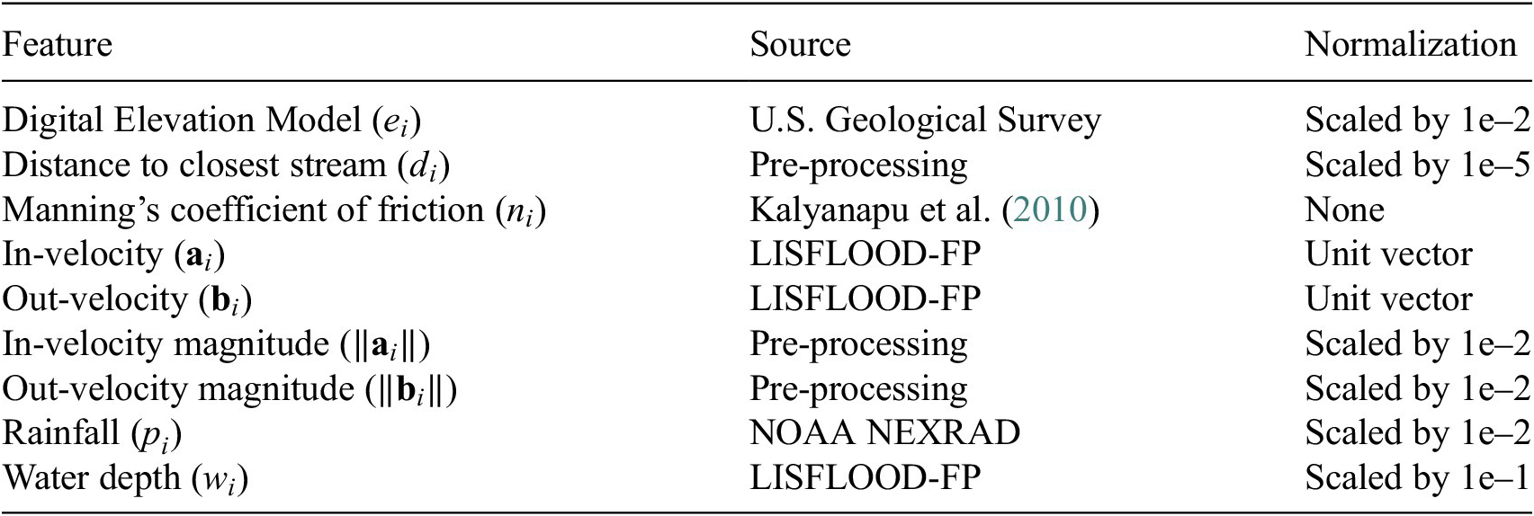
. We consider the ground elevation
$ \left({\mathbf{a}}_i^{t-k},{\mathbf{b}}_i^{t-k}\right),\dots, \left({\mathbf{a}}_i^{t-1},{\mathbf{b}}_i^{t-1}\right),\left({\mathbf{a}}_i^t,{\mathbf{b}}_i^t\right) $
. We consider the ground elevation $ {e}_i $
, the Manning friction coefficient
$ {e}_i $
, the Manning friction coefficient $ {n}_i $
, and the distance to the closest river
$ {n}_i $
, and the distance to the closest river $ {d}_i $
as static topographic attributes (see Figure 2). Moreover, rainfall predictions
$ {d}_i $
as static topographic attributes (see Figure 2). Moreover, rainfall predictions $ {p}_i^t $
, which will impact predicted depths and velocities, are given for each location. We note that our model is general enough to account for other static features, including those derived from the set we have considered (e.g., slope and aspect). We do not consider features with spatial information such as the absolute location of nodes, which can violate the rotation-invariance property of the graph representation. Our goal is to provide a compact set of features to the model and allow it to learn more complex (composite) features directly from data.
$ {p}_i^t $
, which will impact predicted depths and velocities, are given for each location. We note that our model is general enough to account for other static features, including those derived from the set we have considered (e.g., slope and aspect). We do not consider features with spatial information such as the absolute location of nodes, which can violate the rotation-invariance property of the graph representation. Our goal is to provide a compact set of features to the model and allow it to learn more complex (composite) features directly from data.
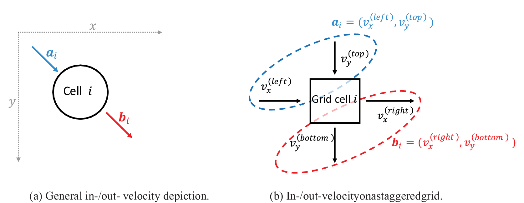
(a) On a general graph, each node/cell $ i $
has an inflow with an in-velocity
$ i $
has an inflow with an in-velocity $ {\mathbf{a}}_i $
and outflow with an out-velocity
$ {\mathbf{a}}_i $
and outflow with an out-velocity $ {\mathbf{b}}_i $
. We note that water can enter and exit the cell in any direction and
$ {\mathbf{b}}_i $
. We note that water can enter and exit the cell in any direction and $ {\mathbf{a}}_i $
and
$ {\mathbf{a}}_i $
and $ {\mathbf{b}}_i $
will differ depending on the properties of node
$ {\mathbf{b}}_i $
will differ depending on the properties of node $ i $
(e.g., friction and elevation). (b) the same vectors can be represented on a staggered grid using (left and top) cell interfaces as a basis for in-velocity
$ i $
(e.g., friction and elevation). (b) the same vectors can be represented on a staggered grid using (left and top) cell interfaces as a basis for in-velocity $ {\mathbf{a}}_i $
and (right and bottom) cell interfaces as a basis for out-velocity. This convention is applied by LISFLOOD-FP (Bates et al., Reference Bates, Trigg and Neal2013).
$ {\mathbf{a}}_i $
and (right and bottom) cell interfaces as a basis for out-velocity. This convention is applied by LISFLOOD-FP (Bates et al., Reference Bates, Trigg and Neal2013).
Input features. Pre-processing means that the data were calculated from other features
Spatial distribution of static features in our dataset.
4. Problem formulation and approach
FloodGNN-GRU is a spatio-temporal model that combines a GNN, named FloodGNN, and a gated recurrent unit (GRU) network (Cho et al., Reference Cho, van Merriënboer, Bahdanau and Bengio2014). Its predictions are based on $ D $
-dimensional dynamics. Vector representations
$ D $
-dimensional dynamics. Vector representations $ {H}^{t+1}\in {\mathrm{\mathbb{R}}}^{n\times D} $
as
$ {H}^{t+1}\in {\mathrm{\mathbb{R}}}^{n\times D} $
as $ {H}^{t+1}=\mathrm{FloodGNN}-\mathrm{GRU}\left({H}^t,{X}^t,G\right) $
, where
$ {H}^{t+1}=\mathrm{FloodGNN}-\mathrm{GRU}\left({H}^t,{X}^t,G\right) $
, where $ n $
is the number of nodes,
$ n $
is the number of nodes, $ {H}^t\in {\mathrm{\mathbb{R}}}^{n\times D} $
are latent representations, used as hidden states in the GRU module (at time
$ {H}^t\in {\mathrm{\mathbb{R}}}^{n\times D} $
are latent representations, used as hidden states in the GRU module (at time $ t $
),
$ t $
), $ {X}^t $
combines node scalar and vector attributes at time
$ {X}^t $
combines node scalar and vector attributes at time $ t $
,
$ t $
, $ G $
is the graph topology (i.e., set of nodes and edges), and
$ G $
is the graph topology (i.e., set of nodes and edges), and $ D $
is a hyperparameter.
$ D $
is a hyperparameter.
4.1. Formulation
We represent the flood dynamics within a grid with states $ {R}_g^1,\dots {R}_g^T $
, where the topology remains constant by the node features change over time. At time
$ {R}_g^1,\dots {R}_g^T $
, where the topology remains constant by the node features change over time. At time $ t $
, the system is in state
$ t $
, the system is in state $ {R}_g^t $
where the nodes (i.e., grid cells)
$ {R}_g^t $
where the nodes (i.e., grid cells) $ {v}_i\in V $
are associated with vector features
$ {v}_i\in V $
are associated with vector features $ {\mathbf{V}}_i^t $
and scalar features
$ {\mathbf{V}}_i^t $
and scalar features $ {\mathbf{s}}_i $
. As vector features, we consider
$ {\mathbf{s}}_i $
. As vector features, we consider $ {\mathbf{V}}_i^t={\left[{\mathbf{a}}_i^t/\parallel {\mathbf{a}}_i^t\parallel, {\mathbf{b}}_i^t/\parallel {\mathbf{b}}_i^t\parallel \right]}^T\in {\mathrm{\mathbb{R}}}^{2\times 2} $
, which are in- and out- velocities (See Figure 1). As scalar features, we consider
$ {\mathbf{V}}_i^t={\left[{\mathbf{a}}_i^t/\parallel {\mathbf{a}}_i^t\parallel, {\mathbf{b}}_i^t/\parallel {\mathbf{b}}_i^t\parallel \right]}^T\in {\mathrm{\mathbb{R}}}^{2\times 2} $
, which are in- and out- velocities (See Figure 1). As scalar features, we consider $ {\mathbf{s}}_i^t={\left({e}_i,{n}_i,{d}_i,\parallel {\mathbf{a}}_i^t\parallel, \parallel {\mathbf{b}}_i^t\parallel, {w}_i^t\right)}^T\in {\mathrm{\mathbb{R}}}^6 $
(see problem definition in Section 3). Our goal is, given the current state
$ {\mathbf{s}}_i^t={\left({e}_i,{n}_i,{d}_i,\parallel {\mathbf{a}}_i^t\parallel, \parallel {\mathbf{b}}_i^t\parallel, {w}_i^t\right)}^T\in {\mathrm{\mathbb{R}}}^6 $
(see problem definition in Section 3). Our goal is, given the current state $ {R}_g^t $
of
$ {R}_g^t $
of $ {R}_g $
, to predict the depth
$ {R}_g $
, to predict the depth $ {w}_i^{t+1} $
and velocity
$ {w}_i^{t+1} $
and velocity $ {\mathbf{V}}_i^{t+1} $
for each node
$ {\mathbf{V}}_i^{t+1} $
for each node $ {v}_i\in V $
at time step
$ {v}_i\in V $
at time step $ t+1 $
.
$ t+1 $
.
4.2. Method
In FloodGNN-GRU, a graph neural network (FloodGNN) captures the spatial behavior of a flooding event as it spreads over a region. This is performed using the message-passing mechanism proposed in (Gilmer et al., Reference Gilmer, Schoenholz, Riley, Vinyals and Dahl2020). The temporal evolution of the flood is captured by a gated recurrent unit (GRU), which is a type of Recurrent Neural Network (Cho et al., Reference Cho, Merrienboer, Gulcehre, Bougares, Schwenk and Bengio2014; Yu et al., Reference Yu, Si, Hu and Zhang2019). These two components of our proposed method are introduced in the three sections following sections.
4.2.1. Spatial information with FloodGNN
FloodGNN represents a given area as a graph by sampling nodes over the space. Topographic and rainfall data from the corresponding area are assigned to each node, and nodes are connected based on spatial adjacency. As velocities are vectors, we would like to preserve their geometry and not treat them as scalar features. Thus, we apply GVP (Jing et al., Reference Jing, Eismann, Suriana, Townshend and Dror2021) for feature transformation with attention mechanism during message passing as proposed by Lu et al. (Reference Lu, Yang, Batra and Parikh2016). GVPs are an extension of standard dense layers (MLPs) that consider two types of features: scalar features $ \left(\mathbf{s}\in {\mathrm{\mathbb{R}}}^C\right) $
and vector features
$ \left(\mathbf{s}\in {\mathrm{\mathbb{R}}}^C\right) $
and vector features $ \left(\mathbf{V}\in {\mathrm{\mathbb{R}}}^{D\times 2}\right) $
. The former is the concatenation of features that by nature are
$ \left(\mathbf{V}\in {\mathrm{\mathbb{R}}}^{D\times 2}\right) $
. The former is the concatenation of features that by nature are $ c $
scalars (e.g., ground elevation) and the latter is a collection of
$ c $
scalars (e.g., ground elevation) and the latter is a collection of $ d $
features that have some physical/geometric properties and are therefore represented as vectors (e.g., velocity in 2D). GVP takes a tuple of scalar features and vector features
$ d $
features that have some physical/geometric properties and are therefore represented as vectors (e.g., velocity in 2D). GVP takes a tuple of scalar features and vector features $ \left(\mathbf{s},\mathbf{V}\right) $
to produce a new tuple of scalar and vector features
$ \left(\mathbf{s},\mathbf{V}\right) $
to produce a new tuple of scalar and vector features $ \left({\mathbf{s}}^{\prime}\in {\mathrm{\mathbb{R}}}^M,{\mathbf{V}}^{\prime}\in {\mathrm{\mathbb{R}}}^{N\times 2}\right) $
.
$ \left({\mathbf{s}}^{\prime}\in {\mathrm{\mathbb{R}}}^M,{\mathbf{V}}^{\prime}\in {\mathrm{\mathbb{R}}}^{N\times 2}\right) $
.
Thus, $ \left({\mathbf{s}}^{\prime },{\mathbf{V}}^{\prime}\right) $
= GVP
$ \left({\mathbf{s}}^{\prime },{\mathbf{V}}^{\prime}\right) $
= GVP $ \left(\mathbf{s},\mathbf{V}\right) $
, slightly modified from Jing et al. (Reference Jing, Eismann, Suriana, Townshend and Dror2021), is defined as follows:
$ \left(\mathbf{s},\mathbf{V}\right) $
, slightly modified from Jing et al. (Reference Jing, Eismann, Suriana, Townshend and Dror2021), is defined as follows:
 $$ {\displaystyle \begin{array}{c}{\mathbf{V}}^{(h)}={\mathbf{W}}_h\mathbf{V}\in {\mathrm{\mathbb{R}}}^{F\times 2}\\ {}{\mathbf{V}}^{\prime }={\mathbf{W}\mathbf{V}}^{(h)}\in {\mathrm{\mathbb{R}}}^{N\times 2}\\ {}\mathbf{r}=\parallel {\mathbf{V}}^{(h)}{\parallel}_2\in {\mathrm{\mathbb{R}}}^F\left(\mathrm{row}\hbox{-} \mathrm{wise}\;\mathrm{L}2\hbox{-} \operatorname{norm}\right)\\ {}\mathbf{q}=\left[\mathbf{r}\parallel \mathbf{s}\right]\in {\mathrm{\mathbb{R}}}^{F+C}\left(\mathrm{concatenation}\right)\\ {}{\mathbf{s}}^{\prime }={\mathbf{W}}_s\mathbf{q}+\mathbf{b}\in {\mathrm{\mathbb{R}}}^M\end{array}} $$
where $ {\mathbf{W}}_h\in {\mathrm{\mathbb{R}}}^{F\times D} $
,
$ {\mathbf{W}}_h\in {\mathrm{\mathbb{R}}}^{F\times D} $
, $ \mathbf{W}\in {\mathrm{\mathbb{R}}}^{N\times F} $
,
$ \mathbf{W}\in {\mathrm{\mathbb{R}}}^{N\times F} $
, $ {\mathbf{W}}_s\in {\mathrm{\mathbb{R}}}^{M\times \left(F+C\right)} $
, and
$ {\mathbf{W}}_s\in {\mathrm{\mathbb{R}}}^{M\times \left(F+C\right)} $
, and $ \mathbf{b}\in {\mathrm{\mathbb{R}}}^M $
are learnable weights. Vector operations (multiplication by a weight matrix) preserve equivariance to vector operations (combinations of rotations and reflections), while the scalar operations are more expressive (vector norms are treated as scalars).
$ \mathbf{b}\in {\mathrm{\mathbb{R}}}^M $
are learnable weights. Vector operations (multiplication by a weight matrix) preserve equivariance to vector operations (combinations of rotations and reflections), while the scalar operations are more expressive (vector norms are treated as scalars).
FloodGNN is therefore similar to traditional GNNs but replaces their simple multiplication by weight matrices (in message passing and update operations) with GVP operations. Given a node $ {v}_i $
with immediate neighborhood
$ {v}_i $
with immediate neighborhood $ \mathcal{N}\left({v}_i\right)=\left\{{v}_i\right\}\cup \left\{{v}_j:\mathrm{there}\ \mathrm{is}\ \mathrm{an}\ \mathrm{edge}\;{v}_j\to {v}_i\right\} $
, the node update operation is performed as follows:
$ \mathcal{N}\left({v}_i\right)=\left\{{v}_i\right\}\cup \left\{{v}_j:\mathrm{there}\ \mathrm{is}\ \mathrm{an}\ \mathrm{edge}\;{v}_j\to {v}_i\right\} $
, the node update operation is performed as follows:
 $$ {\displaystyle \begin{array}{c}\left({\mathbf{p}}_j,{\mathbf{P}}_j\right)=\mathrm{GVP}\left({\mathbf{s}}_j,{\mathbf{V}}_j\right)\hskip2em \forall {v}_j\in \mathcal{N}\left({v}_i\right)\\ {}{\mathbf{s}}_i^{\prime }=\sum \limits_{j\mid {v}_j\in \mathcal{N}\left({v}_i\right)}{\alpha}_j{\mathbf{p}}_j,\hskip2em {\mathbf{V}}_i^{\prime }=\sum \limits_{j\mid {v}_j\in \mathcal{N}\left({v}_i\right)}{\beta}_j{\mathbf{P}}_j\end{array}} $$
The scalars $ {\alpha}_j $
and
$ {\alpha}_j $
and $ {\beta}_j $
are attention weights assigned to
$ {\beta}_j $
are attention weights assigned to $ {v}_j $
when passing message to
$ {v}_j $
when passing message to $ {v}_i $
(Li, Reference Li2022):
$ {v}_i $
(Li, Reference Li2022):
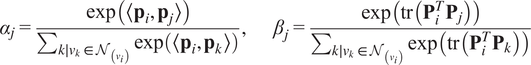 $$ {\alpha}_j=\frac{\exp \left(\left\langle {\mathbf{p}}_i,{\mathbf{p}}_j\right\rangle \right)}{\sum_{k\mid {v}_k\in {\mathcal{N}}_{\left({v}_i\right)}}\exp \left(\left\langle {\mathbf{p}}_i,{\mathbf{p}}_k\right\rangle \right)},\hskip2em {\beta}_j=\frac{\exp \left(\mathrm{tr}\left({\mathbf{P}}_i^T{\mathbf{P}}_j\right)\right)}{\sum_{k\mid {v}_k\in {\mathcal{N}}_{\left({v}_i\right)}}\exp \left(\mathrm{tr}\left({\mathbf{P}}_i^T{\mathbf{P}}_k\right)\right)} $$
where $ \left\langle \cdot \right\rangle $
is the inner product between two vectors and
$ \left\langle \cdot \right\rangle $
is the inner product between two vectors and $ tr\left(\cdot \right) $
is the trace of a matrix:
$ tr\left(\cdot \right) $
is the trace of a matrix:
During training, FloodGNN learns to generate representations ( $ {\mathbf{s}}^{\prime },{\mathbf{V}}^{\prime } $
) that capture the state of the flooding event (i.e., water depths and velocity vectors). In the next section, we describe how a GRU can be combined with FloodGNN to enable it to capture the dynamics of the flooding event.
$ {\mathbf{s}}^{\prime },{\mathbf{V}}^{\prime } $
) that capture the state of the flooding event (i.e., water depths and velocity vectors). In the next section, we describe how a GRU can be combined with FloodGNN to enable it to capture the dynamics of the flooding event.
4.2.2. Spatio-temporal information with GRU and FloodGNN
FloodGNN-GRU applies a GRU model to capture the temporal information from the flooding event. The MLP module from the (traditional) GRU is replaced with FloodGNN layers to leverage the temporal and spatial spread of a flood. Our approach follows a similar strategy to the ConvLSTM architecture (Zhang et al., Reference Zhang, Zhu, Mei, Shen, Shah, Bennamoun, Bengio, Wallach, Larochelle, Grauman, Cesa-Bianchi and Garnett2018) to combine spatial and temporal information, but FloodGNN plays the role of the Convolutional Neural Network. This enables our approach to process a sequence of relevant node inputs (topographic attributes, rainfall, previous water depths, etc.) to predict the next state of the flooding event (water depths and velocity vectors).
The GRU is designed as follows:
 $$ {z}^t=\mathrm{sigmoid}\left({f}_z\left({R}_g^t\right)+{g}_z\left({H}^{t-1}\right)\right) $$
 $$ {r}^t=\mathrm{sigmoid}\left({f}_r\left({R}_g^t\right)+{g}_r\left({H}^{t-1}\right)\right) $$
 $$ {\hat{H}}^t=\tanh \left({f}_h\left({R}_g^t\right)+{g}_h\left({r}_t\hskip0.3em \odot \hskip0.4em {H}^{t-1}\right)\right) $$
 $$ {H}^t={z}^t\hskip0.4em \odot \hskip0.4em {H}^{t-1}+\left(1-{z}^t\right)\hskip0.4em \odot \hskip0.4em {\hat{H}}^t $$
where $ {f}_{\left\{z,r,h\right\}} $
and
$ {f}_{\left\{z,r,h\right\}} $
and $ {g}_{\left\{z,r,h\right\}} $
are FloodGNN layers (see Section 4.2.1) and sigmoid and tanh are non-linear activation functions.
$ {g}_{\left\{z,r,h\right\}} $
are FloodGNN layers (see Section 4.2.1) and sigmoid and tanh are non-linear activation functions. $ {R}_g^t $
is the state of the graph at time t, that is, the set of tuples of scalar features and vector features of all the nodes in the graph at time step
$ {R}_g^t $
is the state of the graph at time t, that is, the set of tuples of scalar features and vector features of all the nodes in the graph at time step $ t $
.
$ t $
. $ {H}^{t-1} $
is the set of tuples of scalar hidden states and vector hidden states from the previous time step
$ {H}^{t-1} $
is the set of tuples of scalar hidden states and vector hidden states from the previous time step $ t-1 $
. Note that all these operations have inputs and output sets as tuples (of scalar and vector features). That is,
$ t-1 $
. Note that all these operations have inputs and output sets as tuples (of scalar and vector features). That is, $ {z}^t,{r}^t,{\hat{H}}^t $
, and
$ {z}^t,{r}^t,{\hat{H}}^t $
, and $ {H}^t $
are all tuples We use
$ {H}^t $
are all tuples We use $ \odot $
as the element-wise product between vectors or matrices. Here again, since we are dealing with tuples,
$ \odot $
as the element-wise product between vectors or matrices. Here again, since we are dealing with tuples, $ \odot $
is applied individually/separately to scalar and vector parts of
$ \odot $
is applied individually/separately to scalar and vector parts of $ {r}^t,{H}^{t-1} $
, and
$ {r}^t,{H}^{t-1} $
, and $ {z}^t $
. Furthermore, all operations, including activation functions and arithmetic operations, are applied individually to the entries of these tuples.
$ {z}^t $
. Furthermore, all operations, including activation functions and arithmetic operations, are applied individually to the entries of these tuples.
4.2.3. Prediction
The values of the water depth $ t+1 $
(
$ t+1 $
( $ {\tilde{w}}_i^{t+1} $
), and associated velocities (
$ {\tilde{w}}_i^{t+1} $
), and associated velocities ( $ {\tilde{\mathbf{a}}}_i^{t+1} $
, and
$ {\tilde{\mathbf{a}}}_i^{t+1} $
, and $ {\tilde{\mathbf{b}}}_i^{t+1} $
) at the next time step are predicted based on node representations as follows:
$ {\tilde{\mathbf{b}}}_i^{t+1} $
) at the next time step are predicted based on node representations as follows:
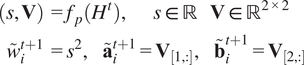 $$ {\displaystyle \begin{array}{c}\left(s,\mathbf{V}\right)={f}_p\left({H}^t\right),\hskip2em s\in \mathrm{\mathbb{R}}\hskip1em \mathbf{V}\in {\mathrm{\mathbb{R}}}^{2\times 2}\\ {}{\tilde{w}}_i^{t+1}={s}^2,\hskip1em {\tilde{\mathbf{a}}}_i^{t+1}={\mathbf{V}}_{\left[1,:\right]},\hskip1em {\tilde{\mathbf{b}}}_i^{t+1}={\mathbf{V}}_{\left[2,:\right]}\end{array}} $$
where $ {f}_p $
is a GVP layer,
$ {f}_p $
is a GVP layer, $ {H}^t $
is defined in Equation 4.4,
$ {H}^t $
is defined in Equation 4.4, $ {\tilde{\mathbf{a}}}_i^{t+1} $
and
$ {\tilde{\mathbf{a}}}_i^{t+1} $
and $ {\tilde{\mathbf{b}}}_i^{t+1} $
are the first row
$ {\tilde{\mathbf{b}}}_i^{t+1} $
are the first row $ \left({\mathbf{V}}_{\left[1,:\right]}\right) $
and second row
$ \left({\mathbf{V}}_{\left[1,:\right]}\right) $
and second row $ \left({\mathbf{V}}_{\left[2,:\right]}\right) $
of
$ \left({\mathbf{V}}_{\left[2,:\right]}\right) $
of $ \mathbf{P} $
, respectively. We take the square of
$ \mathbf{P} $
, respectively. We take the square of $ s $
to obtain
$ s $
to obtain $ {\tilde{w}}_i^{t+1} $
to enforce water depths to always be non-negative.
$ {\tilde{w}}_i^{t+1} $
to enforce water depths to always be non-negative.
The values $ {\tilde{w}}_i^{t+1} $
,
$ {\tilde{w}}_i^{t+1} $
, $ {\tilde{\mathbf{a}}}_i^{t+1} $
and
$ {\tilde{\mathbf{a}}}_i^{t+1} $
and $ {\tilde{\mathbf{b}}}_i^{t+1} $
are used to construct input features
$ {\tilde{\mathbf{b}}}_i^{t+1} $
are used to construct input features $ {\mathbf{s}}_i^{t+1} $
and
$ {\mathbf{s}}_i^{t+1} $
and $ {\mathbf{V}}_i^{t+1} $
, which are used together with
$ {\mathbf{V}}_i^{t+1} $
, which are used together with $ {H}_t $
at the next time-step (
$ {H}_t $
at the next time-step ( $ t+2 $
). The L1 loss, which performed better than L2 loss (see Figure 10), is used to compare predictions
$ t+2 $
). The L1 loss, which performed better than L2 loss (see Figure 10), is used to compare predictions $ {\tilde{w}}_i^{t+1} $
,
$ {\tilde{w}}_i^{t+1} $
, $ {\tilde{\mathbf{a}}}_i^{t+1} $
,
$ {\tilde{\mathbf{a}}}_i^{t+1} $
, $ {\mathbf{b}}_i^{t+1} $
and their respective ground truth values
$ {\mathbf{b}}_i^{t+1} $
and their respective ground truth values $ {w}_i^{t+1} $
,
$ {w}_i^{t+1} $
, $ {\mathbf{a}}_i^{t+1} $
,
$ {\mathbf{a}}_i^{t+1} $
, $ {\mathbf{b}}_i^{t+1} $
to update the model parameters. By minimizing the loss for a training set, we optimize both the FloodGNN and GRU parameters in an end-to-end fashion. Once the model is trained, predictions can be made efficiently based on forward operations.
$ {\mathbf{b}}_i^{t+1} $
to update the model parameters. By minimizing the loss for a training set, we optimize both the FloodGNN and GRU parameters in an end-to-end fashion. Once the model is trained, predictions can be made efficiently based on forward operations.
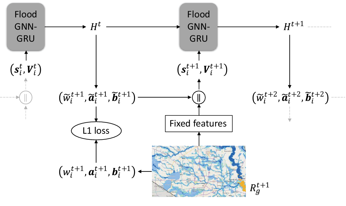
The overall architecture of FloodGNN-GRU is shown in Figure 3. FloodGNN-GRU can predict the dynamics of flooding events based on both topographic attributes and rainfall forecasts. In particular, the recursive nature of our model, inherited from the GRU architecture, enables it to make predictions with long-term lead times—i.e., number of time steps in the future. In the next section, we will evaluate our model using a representative dataset from Hurricane Harvey, in Houston, TX.
Overview of FloodGNN-GRU. At each time $ t $
, the region
$ t $
, the region $ {R}_g $
is in state
$ {R}_g $
is in state $ {R}_g^t $
with scalar features
$ {R}_g^t $
with scalar features $ {\mathbf{s}}_i^t $
and vector features
$ {\mathbf{s}}_i^t $
and vector features $ {\mathbf{V}}_i^t $
for each node/cell
$ {\mathbf{V}}_i^t $
for each node/cell $ {v}_i $
. These are processed through a FloodGNN-GRU to produce hidden state
$ {v}_i $
. These are processed through a FloodGNN-GRU to produce hidden state $ {H}^t $
that captures both spatial and temporal information on the dynamics of a flooding event.
$ {H}^t $
that captures both spatial and temporal information on the dynamics of a flooding event. $ {H}^t $
is later used for the estimation of the next water depth
$ {H}^t $
is later used for the estimation of the next water depth $ {\tilde{w}}_i^{t+1} $
and velocities
$ {\tilde{w}}_i^{t+1} $
and velocities $ {\tilde{\mathbf{a}}}_i^{t+1} $
and
$ {\tilde{\mathbf{a}}}_i^{t+1} $
and $ {\tilde{\mathbf{b}}}_i^{t+1} $
. The L1 loss function between
$ {\tilde{\mathbf{b}}}_i^{t+1} $
. The L1 loss function between $ {\tilde{w}}_i^{t+1} $
,
$ {\tilde{w}}_i^{t+1} $
, $ {\tilde{\mathbf{a}}}_i^{t+1} $
,
$ {\tilde{\mathbf{a}}}_i^{t+1} $
, $ {\tilde{\mathbf{b}}}_i^{t+1} $
and their ground truth values
$ {\tilde{\mathbf{b}}}_i^{t+1} $
and their ground truth values $ {w}_i^{t+1} $
,
$ {w}_i^{t+1} $
, $ {\mathbf{a}}_i^{t+1} $
,
$ {\mathbf{a}}_i^{t+1} $
, $ {\mathbf{b}}_i^{t+1} $
is used for parameter learning in our model.
$ {\mathbf{b}}_i^{t+1} $
is used for parameter learning in our model.
5. Experiments
This section provides an empirical evaluation of FloodGNN-GRU, which is our data-driven approach for flood prediction that combines a GNN and a GRU architecture. The goal of our evaluation is to address the following questions: (1) how accurate is FloodGNN-GRU at predicting water depths for various lead times compared to alternative data-driven approaches and (2) how efficiently can FloodGNN-GRU be trained and tested compared to a traditional physics-based inundation model?
5.1. Dataset
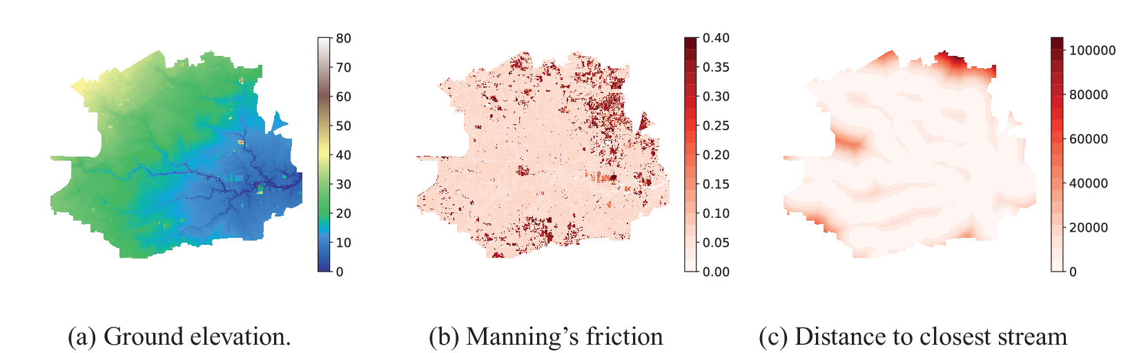
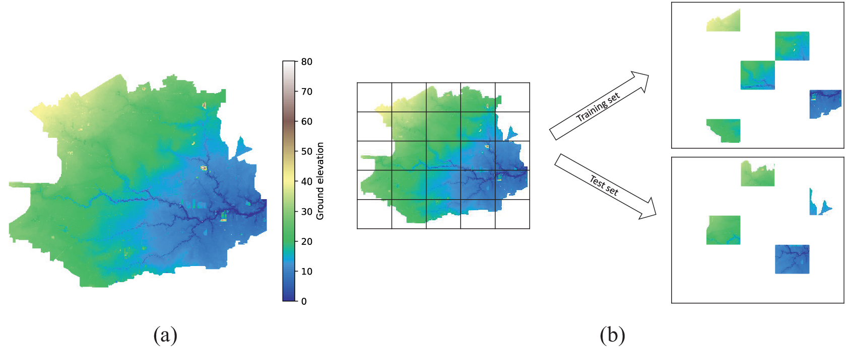
Our experiments are based on simulations from the grid-based flood inundation model LISFLOOD-FP (version 8) (Bates, Reference Bates2013). The model domain was designated using a modified shapefile of the Harris County Flood Control District’s (HCFCD) watershed boundaries as a mask. Elevation data were interpolated onto the model grid using a 10-m digital elevation model (DEM) collected from the U.S. Geological Survey’s (USGS) 3D Elevation Program (3DEP) national elevation dataset (NED). River bathymetry data (i.e., bed elevation, bank elevation, channel width) were extracted from HEC-RAS models maintained by HCFCD and available via the Model and Map Management (M3) System and used to create the sub-grid channels (SGC) embedded within the model domain. Overland roughness coefficients were assigned to each grid cell based on the land use/land cover (LULC) classes in the 2016 multi-resolution land characteristics (MLRC) Consortium’s National Land Cover Database (NLCD), which classifies 16 land cover types at a 30-m resolution for the CONUS. Manning’s friction coefficients were obtained for each LULC class from Kalyanapu et al. (Reference Kalyanapu, Burian and McPherson2010). Infiltration was assumed to be spatially uniform across the model domain (1.5E-6 ms−1). The final 30-m resolution model contains 3,208,196 (1961 $ \times $
1636) active grid cells and encompasses a large portion of Harris County and the City of Houston (Figure 4a).
$ \times $
1636) active grid cells and encompasses a large portion of Harris County and the City of Houston (Figure 4a).
(a) Digital elevation model (DEM) of Houston, Texas. (b) Generation of non-overlapping sub-regions and illustrative example of the split of these sub-regions into training and test sets.
To validate the LISFLOOD-FP model performance, we hindcast Hurricane Harvey for 6 days beginning on August 25, 2017, 00:00 UTC. Runoff processes were simulated by forcing the model with observed precipitation and streamflow. Hourly NOAA NEXRAD radar precipitation records were obtained from the Multi-Radar Multi-Sensor Gauge Corrected (MRMS-GC) Quantitative Precipitation Estimation (QPE) product (Martinaitis et al., Reference Martinaitis, Osborne, Simpson, Zhang, Howard, Cocks, Arthur, Langston and Kaney2020; https://github.com/dossgollin-lab/climate-data/). Upstream boundary conditions were included at the outlets of Addicks and Barker reservoirs using reported hydrographs at USGS streamflow gages 08072600 and 08073100 and at the eastern boundary of the model domain using observed water level records at the NOAA tide gage located at Manchester (Station ID: 8770777). The simulation was run using an adaptive time stepping algorithm based on the convergence condition by Courant–Friedrichs–Lewy to ensure stability and convergence, and gridded water levels were saved every 3600 seconds during the simulation. We compare modeled and observed water levels at 73 USGS high water marks (HWMs) and calculate a root-mean-square-error (RMSE) of 1.07, bias (also known as mean error) of 0.82, and R 2 of 0.98.
Using the validated model, we obtained hourly water depths and velocity vectors (i.e., time series with a time-step of 1 hour). The model domain was divided into smaller non-overlapping sub-regions of sizes $ \approx 50\times 32 $
to generate enough sample regions for training (illustrated in Figure 4b) the baselines and our proposed model. The models are trained and tested on different sub-regions to simulate the setting where our model is applied as an alternative LISFLOOD-FP. The simulation outputs from LISFLOOD-FP are, thus, considered as ground truth or true water depths/velocities for training as well as testing in our work. We obtained the graph representations of these regions by considering a grid cell as a node that is linked to its surrounding cells. There were 1531 grid-based (non-overlapping) sub-regions from which we randomly selected
$ \approx 50\times 32 $
to generate enough sample regions for training (illustrated in Figure 4b) the baselines and our proposed model. The models are trained and tested on different sub-regions to simulate the setting where our model is applied as an alternative LISFLOOD-FP. The simulation outputs from LISFLOOD-FP are, thus, considered as ground truth or true water depths/velocities for training as well as testing in our work. We obtained the graph representations of these regions by considering a grid cell as a node that is linked to its surrounding cells. There were 1531 grid-based (non-overlapping) sub-regions from which we randomly selected $ 70\% $
for training,
$ 70\% $
for training, $ 15\% $
for validation, and
$ 15\% $
for validation, and $ 15\% $
for testing. We randomly split the data to avoid having in one split, say, training split, regions with one predominantly common feature (for instance, all flat areas); we further consider three random independent splits, resulting in three experiment results (See Section 5.3).
$ 15\% $
for testing. We randomly split the data to avoid having in one split, say, training split, regions with one predominantly common feature (for instance, all flat areas); we further consider three random independent splits, resulting in three experiment results (See Section 5.3).
The generated flood inundation data is heavily left-skewed, that is, a majority of water depths are zero. This causes some challenges to the training process of a machine learning model such as back-propagation of gradient zero. Therefore, to remove the excessive number of (leading) zeroes from the data, for each sample sub-region, we start counting the first time step where there is at least one grid cell with a non-zero water depth value. 1 shows features used in our experiments and the normalization employed for each one of them. In most cases, feature values are scaled down by their order of magnitude. For instance, rainfall values can be of 2 orders of magnitude; thus, they are multiplied by 1e-2.
5.2. Evaluation metrics
We used metrics commonly employed in regression tasks for the evaluation of and comparison between the performances of our proposed method and baselines. In the notation used below, $ {y}_i $
is the true water depth of a cell,
$ {y}_i $
is the true water depth of a cell, $ {p}_i $
is the predicted water depth of the cell,
$ {p}_i $
is the predicted water depth of the cell, $ {\overline{y}}_i $
is the mean of water depth over all the cells, and
$ {\overline{y}}_i $
is the mean of water depth over all the cells, and $ N $
is the total number of all the cells (from all the sub-regions combined). While comparing the methods based on a single evaluation metric might not be sufficient, this comprehensive set of metrics, in combination, provides a clear picture of their performance.
$ N $
is the total number of all the cells (from all the sub-regions combined). While comparing the methods based on a single evaluation metric might not be sufficient, this comprehensive set of metrics, in combination, provides a clear picture of their performance.
-
• Root mean square error:
 $$ \mathrm{RMSE}=\sqrt{\frac{1}{N}\parallel {y}_i-{p}_i{\parallel}_2^2} $$
-
• Nash–Sutcliffe model efficiency coefficient:
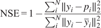 $$ \mathrm{NSE}=1-\frac{\sum_i^N\parallel {y}_i-{p}_i{\parallel}_2^2}{\sum_i^N\parallel {y}_i-{\overline{y}}_i{\parallel}_2^2} $$
-
• Pearson correlation coefficient:
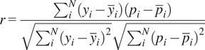 $$ r=\frac{\sum_i^N\left({y}_i-{\overline{y}}_i\right)\left({p}_i-{\overline{p}}_i\right)}{\sqrt{\sum_i^N{\left({y}_i-{\overline{y}}_i\right)}^2}\sqrt{\sum_i^N{\left({p}_i-{\overline{p}}_i\right)}^2}} $$
-
• Symmetric mean absolute percentage error. This is an alternative to MAPE (mean absolute percentage error) which tends to blow up to infinity when the true data has zero values:
 $$ \mathrm{sMAPE}=\frac{1}{N}\sum \limits_i^N\frac{\mid {y}_i-{p}_i\mid }{\mid {y}_i\mid +\mid {p}_i\mid } $$
-
• Critical success index
 $$ \mathrm{CSI}=\frac{\mathrm{TP}}{\mathrm{TP}+\mathrm{FP}+\mathrm{FN}} $$
where TP are true positives (cells with both the predictions and ground truths greater than $ \gamma $
), FP are false positives (cells whose ground truths are less than
$ \gamma $
), FP are false positives (cells whose ground truths are less than $ \gamma $
but the model’s predictions are greater than
$ \gamma $
but the model’s predictions are greater than $ \gamma $
), and FN are false negatives (cells where the model fail to predict a flooded area). In our experiments, we consider
$ \gamma $
), and FN are false negatives (cells where the model fail to predict a flooded area). In our experiments, we consider $ \gamma =0.001\;\mathrm{m} $
which is the lowest positive value possible.
$ \gamma =0.001\;\mathrm{m} $
which is the lowest positive value possible.
5.3. Results
We compare our method against the following baseline methods.
-
• GCN-GRU: This model is similar to FloodGNN-GRU, but we simply use a graph convolution network (GCN) (Kipf and Welling, Reference Kipf and Welling2017) that processes velocities and scalar features by concatenating them with other features. This method will also serve as part of our ablation analysis evaluating the impact of vector feature representations.
-
• MLP-GRU: This model is also similar to FloogGNN-GRU, but we use a one-layer multi-layer perceptron (MLP) instead of a GNN layer. As a consequence, this model does not consider the spatial model.
-
• Unet: This model is based on the U-Net architecture proposed by Ronneberger et al. (Reference Ronneberger, Fischer and Brox2015) to explicitly account for the temporal behavior of a system.
These baselines are representative methods from the literature on machine learning for flood prediction, which include CNN-based methods (Löwe et al., Reference Löwe, Böhm, Jensen, Leandro and Rasmussen2021; Guo et al., Reference Guo, Leitao, Simões and Moosavi2021; Kabir et al., Reference Kabir, Patidar, Xia, Liang, Neal and Pender2020) and RNN-based methods (Fang et al., Reference Fang, Wang, Peng and Hong2021; Hu et al., Reference Hu, Fang, Pain and Navon2019).
FloodGNN-GRU was trained using the Adam optimizer (Kingma and Ba, Reference Kingma and Ba2015) with weight decay and learning rate set to 1e-3. The model was trained for 1000 epochs during which we kept the best-performing state (weights) of our model based on the lowest RMSE score on the validation set. We performed three independent experiments based on three random splits of the data (as described in Section 5.1). For a fair comparison, the baseline methods were trained and tested on the same data splits as our method.
Table 2 shows the means and standard deviations (over 3 independent experiments) of the metric scores for predictions with lead times of 1, 5, and 10 hours. All the methods were trained and validated (using the validation set) for a total of 8 time steps, but the inference is not restricted to a fixed number of time steps. We found that training on fewer time steps than 8 did not perform well at inference time, and we did not notice much improvement when training using a number of time steps greater than 8. The results show that FloodGNN-GRU achieves the best results across different metrics. Based on the results at time $ t=10 $
, there is a gain of about 17% in terms of RMSE, and 15% in terms of sMAPE, showing that FloodGNN-GRU’s prediction of water depth values is the closest to the true water depths. We can also notice that FloodGNN-GRU has a very high NSE score (about 77% increase), proving that FloodGNN-GRU is not just predicting the trivial mean value of water depth values. The 31% increase in Pearson’s coefficient of correlation score indicates that FloodGNN-GRU’s predictions follow the trend of the ground truth better than competing baselines.
$ t=10 $
, there is a gain of about 17% in terms of RMSE, and 15% in terms of sMAPE, showing that FloodGNN-GRU’s prediction of water depth values is the closest to the true water depths. We can also notice that FloodGNN-GRU has a very high NSE score (about 77% increase), proving that FloodGNN-GRU is not just predicting the trivial mean value of water depth values. The 31% increase in Pearson’s coefficient of correlation score indicates that FloodGNN-GRU’s predictions follow the trend of the ground truth better than competing baselines.
Predictions time-step of size 1-h
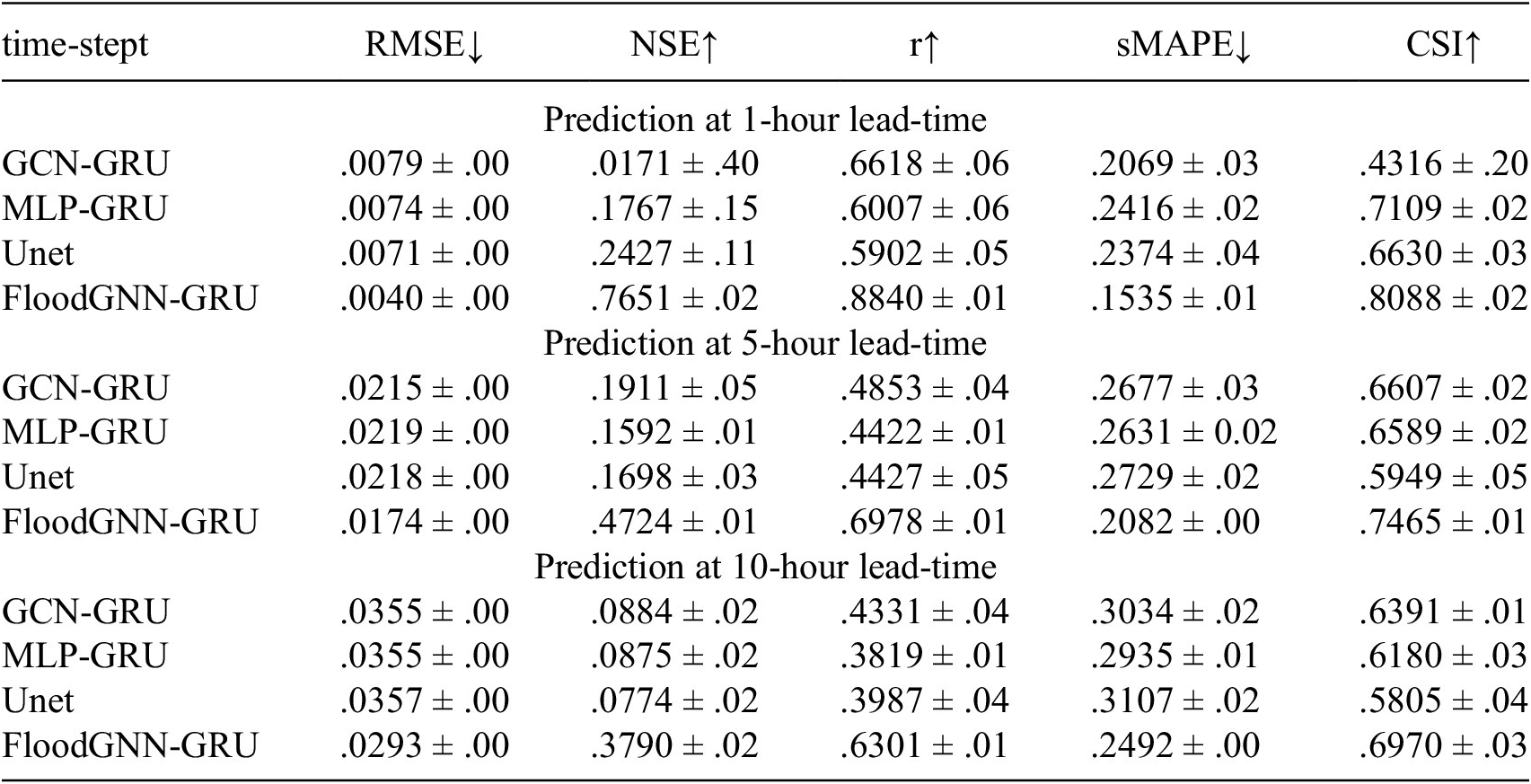
For each metric, the mean and standard deviation over 3 random, independent experiments are provided. RMSE is in meters; while the rest of the metrics are unitless. $ \downarrow $
means lower is better, and
$ \downarrow $
means lower is better, and $ \uparrow $
means higher is better.
$ \uparrow $
means higher is better.
The results of the velocity predictions are shown in Table 3. Here again, we can see that FloodGNN-GRU performs the best, with an RMSE of one order of magnitude less than the second-best approach. This can be attributed to the fact FloodGNN-GRU treats velocities as physical entities by representing them as vector features instead of scalar features.
RSME on the velocity predictions in terms of mean and standard deviation values over 3 random, independent experiments
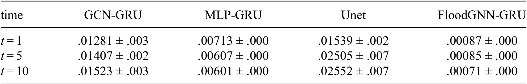
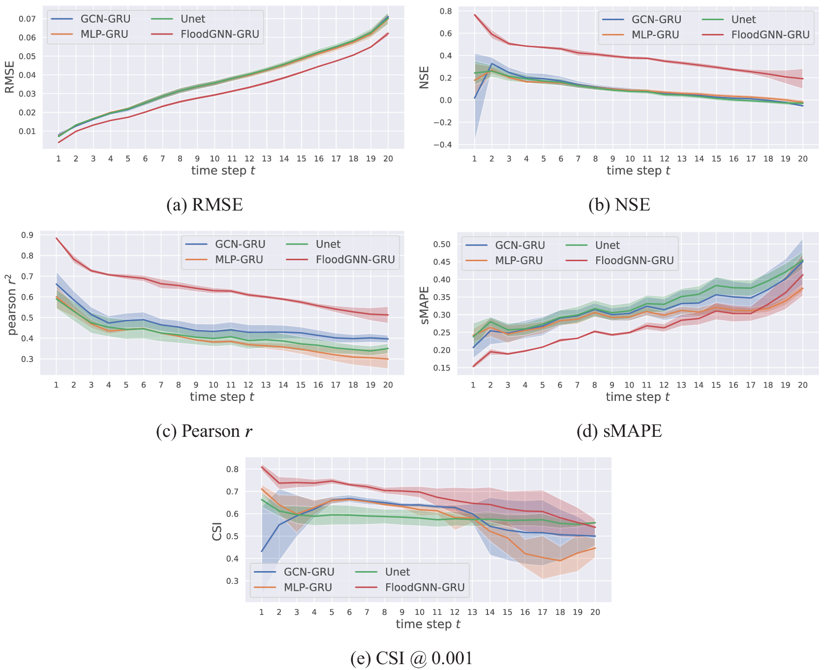
Figure 5 shows the performances of all the methods over longer lead times (from $ t=1 $
to
$ t=1 $
to $ t=20 $
). As expected, the error of the predictions for all methods increases significantly with the lead time. This is due to the accumulation of prediction errors by the recursive model over time. Still, we can observe that FloodGNN-GRU achieves the best results among the approaches considered. As a future work, we will investigate how to incorporate some of the physics of flooding—i.e., the fluid mechanics equations—into our model as a means to improve its long-term accuracy.
$ t=20 $
). As expected, the error of the predictions for all methods increases significantly with the lead time. This is due to the accumulation of prediction errors by the recursive model over time. Still, we can observe that FloodGNN-GRU achieves the best results among the approaches considered. As a future work, we will investigate how to incorporate some of the physics of flooding—i.e., the fluid mechanics equations—into our model as a means to improve its long-term accuracy.
Predictions from time $ t=1 $
to
$ t=1 $
to $ t=20 $
(in hours) with 1-hour time intervals. Each solid line represents the mean over three experiments, and the shadows along the solid lines represent standard deviations. The results show that FloodGNN-GRU achieves the best results compared to other methods.
$ t=20 $
(in hours) with 1-hour time intervals. Each solid line represents the mean over three experiments, and the shadows along the solid lines represent standard deviations. The results show that FloodGNN-GRU achieves the best results compared to other methods.
Figures 6, 7, and 8 provide visualizations of the correlation between true and predicted values—with respective Pearson’s correlation coefficient—at time $ t=1 $
,
$ t=1 $
, $ t=5 $
, and
$ t=5 $
, and $ t=10 $
, respectively, for FloodGNN-GRU and the baselines. The results confirm that FloodGNN-GRU produces the predictions that are the most aligned with the ground truth. However, as noticed earlier, the degradation of the performance is noticeable as the lead time increases. These results also illustrate how all the ML models tend to underestimate larger values of water depth. This is an indication that ML models for flood prediction still need to be improved for extreme events.
$ t=10 $
, respectively, for FloodGNN-GRU and the baselines. The results confirm that FloodGNN-GRU produces the predictions that are the most aligned with the ground truth. However, as noticed earlier, the degradation of the performance is noticeable as the lead time increases. These results also illustrate how all the ML models tend to underestimate larger values of water depth. This is an indication that ML models for flood prediction still need to be improved for extreme events.
Scatter plot of water depths in log–log scale at time $ t=1 $
. FloodGNN-GRU produces predictions that are the most aligned with true values. Pearson’s coefficient of correlation values are given at the bottom of each plot.
$ t=1 $
. FloodGNN-GRU produces predictions that are the most aligned with true values. Pearson’s coefficient of correlation values are given at the bottom of each plot.
Scatter plot of water depths in log–log scale at time $ t=5 $
. FloodGNN-GRU produces predictions that are the most aligned with true values. Pearson’s coefficient of correlation values are given at the bottom of each plot.
$ t=5 $
. FloodGNN-GRU produces predictions that are the most aligned with true values. Pearson’s coefficient of correlation values are given at the bottom of each plot.
Scatter plot of water depths in log–log scale at time $ t=10 $
. FloodGNN-GRU produces predictions that are the most aligned with true values. Pearson’s coefficient of correlation values are given at the bottom of each plot.
$ t=10 $
. FloodGNN-GRU produces predictions that are the most aligned with true values. Pearson’s coefficient of correlation values are given at the bottom of each plot.
To further assess the accuracy of FloodGNN-GRU, Figure 9 shows visualizations of the true water depth and water depth values predicted by our model over a sub-region sampled from the test dataset for lead times $ t=5 $
,
$ t=5 $
, $ t=10 $
, and
$ t=10 $
, and $ t=20 $
. We can see that FloodGNN-GRU follows the trend of the flooding event represented by the true water depth. However, some of the water depths are underestimated by our model. In other words, FloodGNN-GRU is better at localizing the flood than at predicting its intensity.
$ t=20 $
. We can see that FloodGNN-GRU follows the trend of the flooding event represented by the true water depth. However, some of the water depths are underestimated by our model. In other words, FloodGNN-GRU is better at localizing the flood than at predicting its intensity.
True water depth in meters (Column 1) compared to FloodGNN-GRU predictions (Column 2), and the water depth difference map (Column 3). Our approach can localize the flood (i.e., locations with larger water depths), but the extent of the flood is often underestimated, which is consistent with the results from Figures 6 to 8. Note that the color scales are different for each time to better appreciate the difference between the target and prediction values at the different water depth levels.
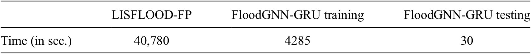
Runtime results: One of the motivations for ML-based flood prediction models is their efficient computation compared to traditional physics-based inundation models. Therefore, we compare the running time of LISFLOOD-FP against the training and test time of FloodGNN-GRU. All the experiments were run on a Linux machine with an Intel(R) Xeon(R) Gold 6342 CPU @ 2.80GHz, 256 GB of RAM, and an NVIDIA GPU Ampere A40. Notice that LISFLOOD was run on the CPU of the same machine. The results are shown in Table 4. FloodGNN-GRU can be trained in 4 min 17 sec per epoch (roughly 1 hour and a half for 1000 epochs) and tested in 30 seconds, which is 1000x faster than the time necessary to run the LISFLOOD-FP simulation. Note that simulations are still needed for training FloodGNN-GRU but are not included in the training time. The most relevant runtime result is for testing, which shows that once trained, FloodGNN-GRU is an efficient alternative to running new LISFLOOD-FP simulations.
Computation times
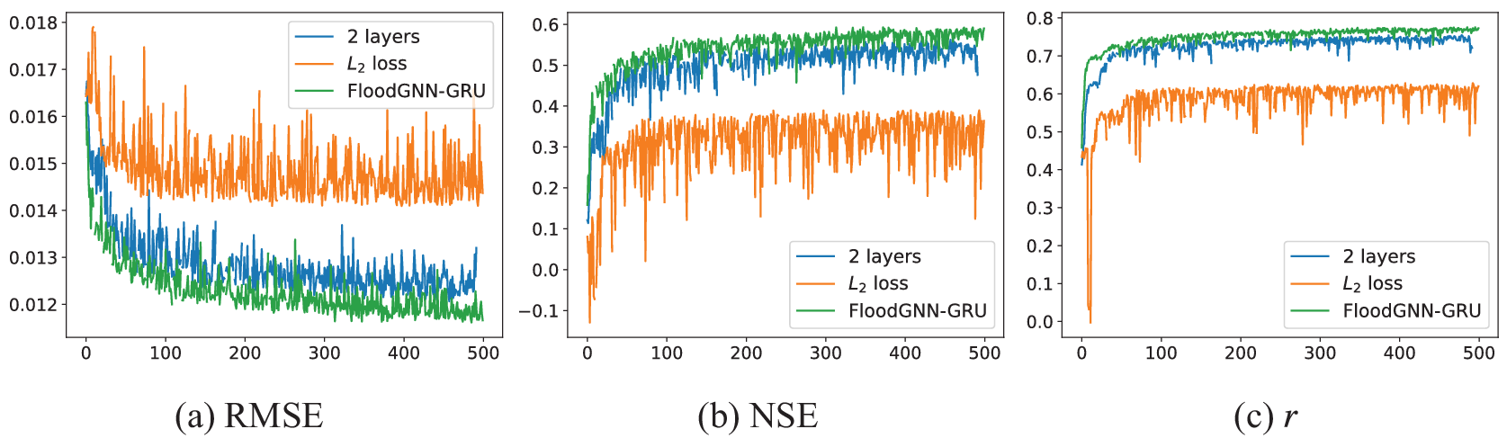
Ablation analysis. Figure 10 shows the performance of FloodGNN-GRU when: (i) we consider 2 FloodGNN layers instead of 1 and (ii) and when we train it with the $ {L}_2 $
loss instead of
$ {L}_2 $
loss instead of $ {L}_1 $
. We can see that a single FloodGNN layer performs better than two layers; thus, adding more layers can hurt performance. Furthermore,
$ {L}_1 $
. We can see that a single FloodGNN layer performs better than two layers; thus, adding more layers can hurt performance. Furthermore, $ {L}_1 $
allows better learning than
$ {L}_1 $
allows better learning than $ {L}_2 $
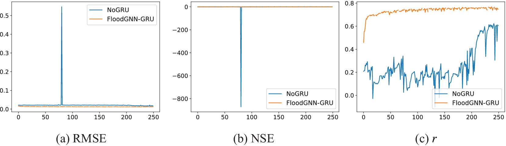
with a significant boost in performance. Figure 11 shows the results when the GRU module is removed from FloodGNN-GRU, we can notice that without the GRU module, the training is not stable and the performance is worsened.
$ {L}_2 $
with a significant boost in performance. Figure 11 shows the results when the GRU module is removed from FloodGNN-GRU, we can notice that without the GRU module, the training is not stable and the performance is worsened.
Performance when FloodGNN-GRU is trained with 2 FloodGNN layers instead of 1, and when it is trained with $ {L}_2 $
loss instead of
$ {L}_2 $
loss instead of $ {L}_1 $
.
$ {L}_1 $
.
Performance when the GRU module of FloodGNN-GRU is removed.
6. Conclusion and future work
We have presented FloodGNN-GRU, a GNN for flood prediction that captures the dynamics of the flooding event using a GRU architecture. FloodGNN-GRU takes as input a spatially distributed rainfall event, static (e.g., ground elevation, friction), and dynamic (e.g., current water depth and velocity vectors) inputs over a region to predict the next water depth and associated velocities. We propose representing velocities as vector features to preserve their physical properties.
Our experiments were based on a realistic LISFLOOD-FP simulation of Hurricane Harvey in Houston, TX. Results have shown that FloodGNN-GRU outperforms three alternative approaches in terms of different evaluation metrics (RMSE, NSE, $ r $
, and sMAP) and for various prediction lead times (from 1 to 20 h). Moreover, the training and testing of FloodGNN-GRU require significantly less time than required for running LISFLOOD-FP simulations, about 1000x faster. These results are strong evidence of the potential of data-driven methods to efficiently emulate physics-based inundation models, especially for short-term predictions.
$ r $
, and sMAP) and for various prediction lead times (from 1 to 20 h). Moreover, the training and testing of FloodGNN-GRU require significantly less time than required for running LISFLOOD-FP simulations, about 1000x faster. These results are strong evidence of the potential of data-driven methods to efficiently emulate physics-based inundation models, especially for short-term predictions.
Our work opens several venues for future research. We will investigate how physics can be incorporated into our model—based on the 2-D shallow water equations (Bates, Reference Bates2022). We will also leverage watershed information to better partition regions for training/testing. Finally, our experiments applied a fixed grid (mesh) topology. We will develop adaptive re-meshing schemes able to select the optimal number of nodes/cells for different areas (e.g., urban versus rural).
Data availability statement
The implementations and datasets used in this work are available at https://github.com/kanz76/FloodGNN-GRU.git.
Author contribution
Conceptualization: A.K., J.D.G, A.Se., A.Si.; Data curation: A.K., J.D.G, A.Se., A.Si.; Formal analysis: A.K., A.Si.; Funding acquisition: A.Si.; Investigation: A.K., A.Si.; Methodology: A.K., J.D.G, A.Se., A.Si.; Software: A.K.; Supervision: A.Si.; Validation: A.K.; Visualization: A.K.; Writing—original draft: A.K., A.Si.; Writing—review and editing: A.K., J.D.G., A.Se., A.Si.
Funding statement
A.K. and A.Si. were supported by a Partners of the Americas US-Brazil 100 K Strong Program Artificial Intelligence for Urban Sustainability and Resilience to Natural Disasters in the Americas and by the U.S. Department of Transportation (USDOT) Tier-1 University Transportation Center (UTC) Transportation Cybersecurity Center for Advanced Research and Education (CYBER-CARE) (grant no. 69A3552348332). A.Se. was supported by the Texas General Land Office (contract No. 19-181-000-B574).
Competing interest
The authors declare no competing interests exist.
Ethics statement
The research meets all ethical guidelines, including adherence to the legal requirements of the study country.


 Open access