
Obesity was probably rare before 1800( Reference Wells 1 ), but by the middle of the nineteenth century it had been identified as a problem and its association with diet and lack of exercise had been recognised( Reference Banting 2 , Reference Bray 3 ). By the year 2000, the global population crossed an historic watershed where for the first time the number of adults carrying excess body weight exceeded the number of those who were underweight( Reference Caballero 4 ). Obesity has continued its inexorable rise in almost all countries( Reference Swinburn, Sacks and Hall 5 ); having more than doubled worldwide since 1980( Reference Haththotuwa, Wijeyaratne, Senarath, Mahmood and Arulkumaran 6 ), it is now considered a pandemic( Reference Swinburn, Sacks and Hall 5 – Reference Popkin, Adair and Ng 8 ).
The problem extends beyond humans. Among companion animals, unprecedented levels of obesity have been reported in recent years for cats (25 %)( Reference Scarlett, Donoghue and Saidla 9 , Reference Zoran 10 ), dogs (33 %)( Reference Zoran 10 , Reference German 11 ) and horses (45 %)( Reference Wyse, McNie and Tannahill 12 , Reference Giles, Rands and Nicol 13 ), and many believe that, as in humans, the rates are increasing( Reference Popkin, Adair and Ng 8 , Reference Hebert, Allison and Archer 14 ). A recent meta-analysis, involving more than 20 000 animals from twenty-four populations, demonstrated positive trends in body weight in recent decades not only in companion animals, but also in primates and rodents living in research colonies, and even feral rodents( Reference Klimentidis, Beasley and Lin 15 ).
What is driving this rising tide of adiposity? The short timescale and synchronised response of several species suggest that the primary cause is a changing environment interacting with biologically susceptible phenotypes. A vast amount of research has been done on a wide range of candidate environmental and biological (physiological, behavioural and psychological) factors, and yet no country has successfully implemented public health measures to reverse the trend of increasing obesity( Reference Swinburn, Sacks and Hall 5 ). It thus seems that new insights and approaches are needed to intervene at the interface where susceptible biology interacts with rapidly changing anthropogenic environments to produce obesity( Reference Hebert, Allison and Archer 14 ).
Nutritional ecology is a branch of biological sciences that aims to understand the role nutrition plays in mediating the relationship between animals and their environments( Reference Klimentidis, Beasley and Lin 15 ), across timescales from short-term homeostatic responses to long-term evolutionary adaptation( Reference Raubenheimer, Simpson and Mayntz 16 ). In recent years, data have accumulated demonstrating that powerful insights can be gained through broadening the conventional focus on the independent effects that nutrients exert on animals, to their interactive effects( Reference Raubenheimer, Simpson and Tait 17 ). For this purpose, we introduced a geometric framework that enables key components of the interaction of the animal (e.g. feeding behaviour, physiology and nutrient requirements) with its environment (e.g. foods) to be represented together in a model and interrelated within the context of multiple nutrients( Reference Simpson and Raubenheimer 18 – Reference Simpson and Raubenheimer 20 ).
To date, the majority of studies using nutritional geometry concern questions and species of interest primarily in the broad context of ecological and evolutionary theory( Reference Simpson and Raubenheimer 18 ). We have, however, also applied this approach to develop and test a new hypothesis about the causes of human obesity, the protein leverage hypothesis (PLH)( Reference Simpson and Raubenheimer 20 – Reference Gosby, Conigrave and Raubenheimer 24 ). This hypothesis differs from traditional approaches in that it emphasises not energy per se, or the contribution of single nutrients such as fats or carbohydrates, but the ways that macronutrients interact to influence energy consumption in changing environments.
The present study aims to introduce nutritional geometry as a general approach for studying the ways that changing environments can influence nutrition-related phenotypes such as metabolic health and obesity, not only in human subjects but also in companion animals and other afflicted species. We do so by showing that the concept of protein leverage can help to explain how human biology interacts with modern environments to produce energy overconsumption, and highlight candidate mechanisms for explaining temporal, geographical and demographic related variances in obesity. We focus on two salient features of the shared environment of humans and human-associated animals, economics and global rises in atmospheric CO2, and also discuss factors that might exacerbate protein leverage through increasing the set point for protein consumption. We close with a discussion of the relevance of nutritional geometry, protein leverage, economics and global atmospheric change to obesity in non-human animals.
Nutritional geometry
Nutritional geometry is a framework for modelling the ways that nutrients and other food components interact in their effects on food choice, food intake and the consequences of feeding, for example in terms of development, health, reproduction and ultimately evolutionary fitness. An important application of this framework is measuring the relative strengths of the feeding regulatory systems for different nutrients, and the ways that these regulatory systems interact to determine diet composition.
The logic underlying this is as follows. If we assume that an animal has evolved feeding regulatory mechanisms that optimise evolutionary fitness within the environment of evolutionary adaptedness( Reference Foley 25 ), then these will cause it to eat a diet that provides the many required nutrients each at its particular target level. Such a diet can be depicted in a geometric model as an intake target – a point or region in a multi-dimensional nutrient space that represents the amounts and ratios of nutrients that are required to be eaten by the animal to maximise fitness (Fig. 1(a)).
Protein–carbohydrate nutrient space for a hypothetical animal and five foods. The intake target (labelled IT) represents the amounts and balance of the two nutrients that are required by the animal over a specified period. ● in (a) show the amounts of the two nutrients in different food items (FIa, FIb and FIc), and the dashed radials (termed nutritional rails) represent the balance of the nutrients in each food. In (b), where there are no points representing specific food items, the nutritional rails represent the balance of the nutrients in the food type – i.e. without specifying a quantity of the food. The solid arrows (T i, T ii and T iii) show the trajectory over which the animal's nutritional state changes as it eats, each being parallel to the nutritional rail for the food being eaten. Food items FIa and FIb contain the same balance of the nutrients as IT – i.e. these foods are nutritionally balanced with respect to protein and carbohydrate. The rail for food c, by contrast, does not pass through IT – i.e. this food in nutritionally imbalanced, and on its own does not allow the animal to reach IT. However, because foods c and d fall on opposite sides of IT, the animal can ‘navigate’ to the target by combining its intake from the two foods – i.e. these foods are nutritionally complementary with respect to nutrients. The sequences of arrows in (b) show two routes, among many possible alternatives, that the animal could take to IT. In (c), the options available to the animal when confined to a single imbalanced food type (food c) are shown. By feeding to intake point I i, it gains the required amount of carbohydrate but suffers a shortfall of protein (P − ); at point I ii, it satisfies its protein needs but over-ingests carbohydrate (C++), and at point I iii, it experiences both a moderate shortage of protein and a moderate excess of carbohydrate. The way that the animal resolves this trade-off between over-ingesting some nutrients and under-ingesting others when restricted to nutritionally imbalanced diets is known as a rule of compromise. (d) To measure rules of compromise, an experiment is performed involving several groups of animals each of which is confined to a food that has a different balance of nutrients and is thus represented by a different nutritional rail. Such an experiment will yield an array of intake points the shape of which reveals the rule of compromise. The vertical array indicates the strategy represented by intake point I ii in (c) (i.e. prioritise protein), and the horizontal array represents the strategy at I i (prioritise carbohydrate). The third array shows an instance where the intake array is asymmetrical – i.e. the response is different for foods containing surplus protein (a negative line) and surplus carbohydrate (an arc). The former, known as the equal distance rule, corresponds with eating to the point on the respective rails where the deficit of one nutrient equals the surplus of the other. The arc, known as the closest distance rule, corresponds with eating to the point on the respective rails that minimises the geometric distance to IT (modified from Simpson & Raubenheimer( Reference Simpson and Raubenheimer 18 )).

One way for an animal to reach the intake target is by selecting a food that contains the nutrients in the same ratio as they are needed – by definition such a food is nutritionally balanced. Foods are represented in geometric models by lines that radiate from the origin at an angle that is determined by the ratio of the nutrients that they contain, called nutritional rails (Fig. 1(a)). When the animal eats, it ingests the nutrients in the same proportion they are present in the food, and its nutritional state can therefore be modelled as ‘moving’ along the nutritional rail over a distance that is proportional to the amount of the food that it eats. Because the ratio of nutrients in a nutritionally balanced food is the same as the target ratio, the nutritional rail for a balanced food intersects the intake target. By eating this food, the animal therefore has a direct route to target and the regulatory challenge is simply to eat enough food to reach the target.
The animal could, alternatively, meet its regulatory target by composing its diet from two or more foods that are nutritionally imbalanced but complementary (Fig. 1(b)). Because neither food intersects the intake target, in this case the regulatory challenge is more complex: it needs to ‘zig-zag’ its way to the target by combining a series of steps none of which on its own would be adequate. To achieve this, regulatory systems are needed that are linked independently to the two nutrients, enabling the animal to switch to the high-protein food with carbohydrate-replete and protein-deficient, and vice versa, and terminate feeding only when the target levels for both nutrients are achieved simultaneously( Reference Raubenheimer, Simpson, Breed and Moore 26 ).
However, if the animal is confined to a food that is imbalanced with respect to particular nutrients, then it cannot reach the intake target but is forced into a trade-off between over-eating some nutrients and under-eating others (Fig. 1(c)). Because both surpluses and deficits of nutrients can have adverse effects( Reference Simpson, Sibly and Lee 27 , Reference Raubenheimer, Lee and Simpson 28 ), evolutionary theory predicts that animals would evolve nutritional systems that regulate the intake of foods to provide the combination of surpluses and deficits that minimises the costs of eating imbalanced foods( Reference Simpson and Raubenheimer 22 , Reference Raubenheimer and Simpson 29 ). In effect, they would evolve appetites for different nutrients each of which is calibrated to achieve a particular balance of surpluses and deficits when the target balance cannot be achieved.
These regulatory dynamics can be measured using experiments in which subjects are provided with one of a range of foods differing in the ratio of the nutrients under investigation and allowed to eat ad libitum over a defined period. Such experiments will yield a geometric pattern of intake points, called an intake array, whose shape will reflect the regulatory rule, or rule of compromise, that the animal uses to resolve the trade-off between over- and under-ingesting nutrients (Fig. 1(d)). In the extreme, if both surpluses and deficits of one nutrient are more costly than surpluses and deficits of others, then the animals should prioritise gaining the target level of that nutrient, even if this involves over- and under-ingesting others. In a two-dimensional model, involving nutrients A and B, the resulting intake array for this scenario would be vertical or horizontal, depending on which nutrient is prioritised, where the variance in intakes of the prioritised nutrient is compressed relative to the other nutrient. A large number of other intake configurations are possible, each reflecting a particular relative weighting of surpluses and deficits of the nutrients( Reference Simpson and Raubenheimer 18 – Reference Simpson and Raubenheimer 20 , Reference Raubenheimer and Simpson 29 ) (Fig. 1(d)).
Protein leverage: macronutrient balance and energy intake in humans
Experiments using nutritional geometry have shown that when eating diets in the range of 10–30 % energy from protein (PE), humans prioritise the intake of PE over non-protein energy (nPE)( Reference Simpson, Batley and Raubenheimer 21 , Reference Gosby, Conigrave and Lau 23 , Reference Martens, Lemmens and Westerterp-Plantenga 30 ). Consequently, energy intake varies inversely with dietary PE:nPE ratio, because fats and carbohydrates are over-eaten to compensate for low PE:nPE ratios and under-eaten on high PE:nPE diets (Fig. 2). A recent meta-analysis involving thirty-eight published ad libitum trials spanning a range of macronutrient ratios and experimental situations confirmed the generality of this response in human subjects( Reference Gosby, Conigrave and Raubenheimer 24 ) (Fig. 3(a)). As predicted, the analysis showed that energy intake varied inversely with dietary protein density across a realistic range of protein densities (Fig. 3(b)). The inverse relationship between protein density and energy intake is particularly apparent in the range of 10–20 % protein. Above 20–25 % protein, the relationship becomes somewhat attenuated presumably due to nPE feedbacks driving an increased intake counterbalancing the negative feedbacks from excess protein( Reference Gosby, Conigrave and Raubenheimer 24 ). Below 10 % protein in the diet, the steeply increasing intakes required to maintain the protein intake become unfeasible( Reference Gosby, Conigrave and Raubenheimer 24 , Reference Martens, Lemmens and Westerterp-Plantenga 30 ). This is not surprising, because such low-protein levels are below values seen naturally in populations with food sufficiency and below even the most extreme estimates of the diets of humans in environments of evolutionary adaptedness (Fig. 4).
Schematic illustration of protein intake regulation and its influence over the intake of non-protein energy. Under strict protein prioritisation (i.e. protein intake is maintained constant), a 1·5 % decrease in the proportion of energy from protein (from 14 to 12·5 %) will result in a 14 % increase in the amount of carbohydrate and fat eaten. Conversely, a 1·5 % decrease in dietary protein density will correspond with a 11 % decrease in non-protein energy eaten. Modified from Simpson & Raubenheimer( Reference Simpson and Raubenheimer 22 ). P, protein; C, carbohydrate; F, fat. (A colour version of this figure can be found online at http://www.journals.cambridge.org/bjn).

(a) Plot of protein (PE) v. non-protein energy (nPE) intakes taken from an analysis of thirty-eight ad libitum studies differing in dietary macronutrient composition, participant age and BMI, study design (menu (![]() ), study shop (
), study shop (![]() ) and diet regimen (
) and diet regimen (![]() )) and study duration(
Reference Gosby, Conigrave and Raubenheimer
24
). The variance along the nPE axis (Y-axis) is much greater than along the PE axis (X-axis) indicating a regulation of protein that is much stronger than the regulation of nPE. This regulation of PE intake drives increased nPE intake when the proportion of protein in the diet is reduced (dashed reference lines represent 10, 15, 25 and 40 % protein diets) to maintain a relatively constant protein (—). (b). Right-angled mixture triangle(
Reference Raubenheimer
48
) showing the relationship between macronutrient distribution (% energy) and energy intake (increasing from dark blue to red). Percentage protein and fat increase along the X and Y axes, respectively. Percentage carbohydrate decreases with distance from the origin, with the grey diagonals (carbohydrate isolines) each representing a fixed percentage carbohydrate (the value given in square brackets). For reference, the points plotting the macronutrient composition of the diets with the lowest protein (●), lowest fat (○) and lowest carbohydrate (
)) and study duration(
Reference Gosby, Conigrave and Raubenheimer
24
). The variance along the nPE axis (Y-axis) is much greater than along the PE axis (X-axis) indicating a regulation of protein that is much stronger than the regulation of nPE. This regulation of PE intake drives increased nPE intake when the proportion of protein in the diet is reduced (dashed reference lines represent 10, 15, 25 and 40 % protein diets) to maintain a relatively constant protein (—). (b). Right-angled mixture triangle(
Reference Raubenheimer
48
) showing the relationship between macronutrient distribution (% energy) and energy intake (increasing from dark blue to red). Percentage protein and fat increase along the X and Y axes, respectively. Percentage carbohydrate decreases with distance from the origin, with the grey diagonals (carbohydrate isolines) each representing a fixed percentage carbohydrate (the value given in square brackets). For reference, the points plotting the macronutrient composition of the diets with the lowest protein (●), lowest fat (○) and lowest carbohydrate (![]() ) are shown, together with the respective (%P:F:C) coordinates. The polygon shows the range of macronutrient ratios recommended in the human diet for reducing the risk of chronic disease: protein = 10–35 %, fat = 20–35 % and carbohydrate = 45–65 %(
31
).
) are shown, together with the respective (%P:F:C) coordinates. The polygon shows the range of macronutrient ratios recommended in the human diet for reducing the risk of chronic disease: protein = 10–35 %, fat = 20–35 % and carbohydrate = 45–65 %(
31
).

Estimated macronutrient intakes of Palaeolithic hunter–gatherers compared with the recommended macronutrient distributions Acceptable Macronutrient Distribution Range (AMDR) for modern humans (yellow polygon, as in Fig. 3(b)). The blue, red and green polygons show estimated possible ranges of proportional macronutrient intakes under four different foraging models presented by Kuipers et al. ( Reference Kuipers, Luxwolda and Dijck-Brouwer 46 ), and the broken-lined black polygon shows the estimated range of intakes from the model of Cordain et al. ( Reference Cordain, Miller and Eaton 44 ). Together, these models encompass a wide range possible ecological and behavioural (e.g. selective v. non-selective feeding) scenarios. The coloured ‘X's show the expected median intakes under the four models of Kuipers et al. ( Reference Kuipers, Luxwolda and Dijck-Brouwer 46 ), and the ■ shows the macronutrient composition for the estimated ‘average Palaeolithic diet’ of Eaton & Konner( Reference Eaton and Konner 120 ). The pink region shows a range of dietary compositions that are not possible for humans, owing to constraints on the maximum rate at which protein can be physiologically processed( Reference Cordain, Miller and Eaton 44 ). Modified from Raubenheimer et al. ( Reference Raubenheimer, Pontzer and Simpson 121 ).

The fact that humans weight protein more heavily than carbohydrates or fats in the regulation of intake led us to propose PLH( Reference Simpson and Raubenheimer 22 ). This model postulates that the strong human appetite for protein has interacted with an ecological shift towards dietary protein dilution to drive rising obesity levels. Conversely, high PE:nPE diets should lead to reduced energy intake and stable or negative energy balance, thus accounting for the efficacy of high-protein weight-loss diets( 31 , Reference Astrup 32 ). Recent evidence from population survey data show, as predicted by PLH, that absolute protein intakes are more stable across time than nPE( Reference Simpson and Raubenheimer 22 , Reference Larsen, Dalskov and Van Baak 33 – Reference Austin, Ogden and Hill 35 ), and decreasing PE:nPE ratios are associated with temporal changes in energy intake and obesity( Reference Martinez-Cordero, Kuzawa and Sloboda 34 ). This suggests that PLH applies not only under experimental conditions, but also in free-living populations. Variation in energy intake and obesity with socioeconomic status (SES)( Reference Austin, Ogden and Hill 35 – Reference McLaren 37 ) is also consistent with PLH, a topic that is further discussed later. As yet, however, the nature of the amino acid signals underlying protein appetite is poorly understood( Reference Simpson and Raubenheimer 18 , Reference Gosby, Conigrave and Raubenheimer 24 ).
It is important in modelling energy and nutrient intakes to distinguish between the different behavioural components of diet selection, namely which foods are chosen from among those available, and the amounts of the chosen foods eaten. PLH is a hypothesis that links the two, by postulating a mechanism for how variation in the protein density of the foods that are eaten (the independent variable), regardless of what causes that variation, will influence energy intake (the dependent variable). If protein leverage has, as postulated, contributed to changes in energy intake and body composition, it thus remains to identify the environmental factors that have driven variation in dietary PE:nPE ratios.
Evolutionary perspectives on protein leverage
An important mechanism through which the environment influences the biology of species is via genetic-level Darwinian evolution, which stems from the differential selection of sequences of DNA. In recent years, however, there has been a broadening of thinking in evolutionary biology to encompass also epigenetic adaptation, which usually operates over shorter timescales than genetic-level evolution. Epigenetic adaptation is based on inheritance of characteristics that are not due to variations in the base sequences of DNA, but are transferred via other mechanisms across generations. Narrow-sense epigenetic inheritance involves heritable modifications to cells, often via the alteration of gene expression, whereas broad-sense epigenetic inheritance may also involve other mechanisms of information transfer, for example via lactation or the social transmission of information( Reference Dinsa, Goryakin and Fumagalli 38 ) that underlies cultural evolution. A perspective that takes into account the interaction of these timescales of evolution is especially important for complex, long-lived species such as human beings where the rate of environmental change can exceed the capacity of genetic-level adaptation( Reference Jablonka and Raz 39 – Reference Odling-Smee, Laland and Feldman 41 ).
Genetic-level evolution
Evidence suggests that the genus Homo spent the majority of its evolution in environments where protein was abundant relative to nPE, especially simple carbohydrates( Reference Gluckman, Hanson and Spencer 42 – Reference Konner and Eaton 45 ) (Fig. 4). In such circumstances, it might be expected that a species would evolve regulatory systems that rank fat and carbohydrate-rich foods as highly palatable, and have a high tolerance for their over-ingestion. Protein, by contrast, should be regulated more tightly if there is a probability both of protein deficit, as would result during food shortages, and of ingesting toxically high levels of protein when food is available but nPE sources are scarce. It is indeed the case that diets with protein in excess of approximately 35–40 % of energy are toxic for humans( Reference Kuipers, Luxwolda and Dijck-Brouwer 46 ) (Fig. 4); by contrast, excess ingested nPE is, in the short-term at least, not toxic and can be stored as fat and drawn on beneficially to ameliorate subsequent energy shortages. This would explain why humans find energy-dense foods to be highly palatable and not highly satiating( Reference Drewnowski 47 ) and why, by contrast, among the macronutrients protein has a particularly strong satiating effect( Reference Raubenheimer 48 , Reference Westerterp-Plantenga, Lejeune and Nijs 49 – Reference Yang and Huffman 51 ). It should be stressed, however, that such adaptive hypotheses need to be tested using phylogenetically controlled comparative analyses( Reference Freckleton, Harvey and Pagel 52 ), but more data on the dynamics of different nutrient systems across a range of species are needed. Comparative studies of macronutrient regulation by phylogenetically and ecologically diverse wild primates have begun, revealing a considerable variation among species in macronutrient prioritisation( Reference Felton, Felton and Raubenheimer 53 – Reference Irwin, Raharison and Raubenheimer 57 ).
Cultural evolution
An evolutionary history of limited nPE, and the associated high palatability of carbohydrates and fats, would predict that a species with the capacity to alter its nutritional ecology through cultural means would do so in a manner that increased the availability of these macronutrients. The multiple independent transitions in the Neolithic to the growing of carbohydrate-rich crops, particularly grains( Reference Cordain and Simopoulos 58 ), and subsequently the farming of relatively fat-rich meats( Reference Cordain, Watkins and Florant 59 ) are consistent with this. So too is the invention during the industrial revolution and subsequent improvement of technologies for the mass production and distribution of refined sugars, starches and vegetable oils( Reference Popkin, Adair and Ng 8 , Reference Mintz 60 ).
The culmination of this trend towards cultural intervention in the human food chain is a category of foods referred to as ultra-processed products( Reference Monteiro, Moubarac and Cannon 61 ). These are products that contain little or no whole foods, but are made from processed substances refined or extracted from whole food (e.g. sugars, flours and starches, oils, hydrogenated oils and fats, and cheap remnants of animal foods). They are typically energy dense and highly palatable with high glycaemic load and salt content, and low in fibre, micronutrients and phytochemicals. Examples include burgers, frozen pasta, pizza and pasta dishes, crisps, cereal bars, biscuits, and carbonated and other sugary drinks( Reference Monteiro, Moubarac and Cannon 61 ).
From an evolutionary perspective, the triumph of these products is that they bypass ecological constraint imposed by the human environment of evolutionary adaptedness on the availability of nPE, concentrating these nutrients into foods that are easily obtained (cheap and highly accessible through vending machines, fast-food chains and supermarkets), rapidly ingested (refined and highly palatable), quickly extracted into the body (easily digested with high glycaemic loads) and readily contribute to positive energy balance (because limited physical activity is required for their acquisition). A somewhat sinister twist, however, is that ultra-processed products not only result directly in an increased intake of nPE, but can also detract from counterbalancing the diet with additional protein. They do this through the addition of savoury flavours that are usually associated with PE-rich foods, thus mimicking complementary foods and deceiving the food selection mechanisms into further intake of nPE( Reference Simpson and Raubenheimer 62 ). The global rise of ultra-processed products, largely driven by powerful trans-national corporations, began in the 1980s and thus coincides closely with the period in which there has been a doubling in the rates of obesity( Reference Haththotuwa, Wijeyaratne, Senarath, Mahmood and Arulkumaran 6 ).
Developmental programming
The integration of genetic-level evolution of feeding regulatory systems and culturally mediated nutritional environments places PLH in a broad evolutionary perspective, where the selection of high nPE foods is due to evolved palatability responses operating in culturally manipulated environments and energy overconsumption is due to tight regulation of protein intake. This long-term perspective does not, however, explain the finer-scaled patterns of energy overconsumption and obesity, for example, its recent rise and differential distribution across and within population groups( Reference Popkin, Adair and Ng 8 ). A set of evolutionary theories has attempted to do this by invoking a form of adaptation that takes place during development termed ‘epigenetic programming’ or ‘developmental programming’. Developmental programming is a variant of phenotypic plasticity, in which the triggering environmental cues are not experienced directly in development but transferred via the mother, for example, through the placenta, lactation or maternal behaviour( Reference Langley-Evans 63 , Reference Sharp, Pickles and Meaney 64 ).
The thrifty phenotype hypothesis( Reference Hales and Barker 65 , Reference Hales and Barker 66 ), and the related ‘predictive adaptive responses’ concept( Reference Gluckman, Hanson and Spencer 42 , Reference Gluckman and Hanson 67 ), propose that a foetus can make developmental adaptations based on signals from the mother predicting the nutritional state of the environment into which it will be born and mature. If the prediction is for an environment with limited food supply, then development is triggered for a phenotype that is energetically thrifty – small, with a low metabolic rate, high insulin sensitivity and a propensity to readily store energy. Such phenotypes have an advantage in conditions of food scarcity, but are vulnerable to obesity and related diseases in energy-rich environments. In this model, developmental programming of the foetus or infant, rather than genetic-level evolution, can account for variance in human susceptibility to obesity, with populations that have encountered a recent shift from energy scarcity to abundance being most vulnerable.
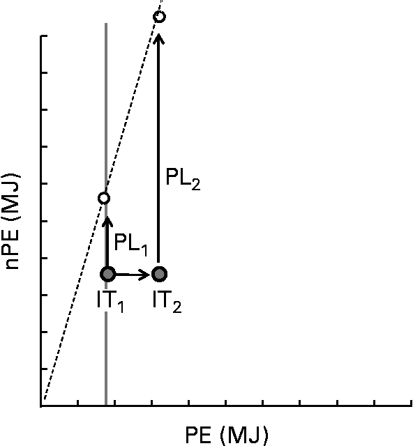
The thrifty phenotype hypothesis is consistent with PLH, in that it might help explain variance in the tendency of human subjects to select foods with low PE:nPE ratios, and also variance in susceptibility to obesity for a given dietary PE:nPE ratio. An interesting question is whether developmental programming might target not only energy regulation per se, but also the regulation of specific nutrients such as protein. We have demonstrated geometrically that protein leverage is accentuated for individuals with high regulatory targets for protein( Reference Simpson and Raubenheimer 22 ), which might be associated with a number of environmental causes and genotypes. One example is that enhanced rates of protein catabolism and hepatic gluconeogenesis can result from overweight and obesity, thus reducing protein efficiency, increasing dietary protein requirements and exacerbating protein leverage( Reference Simpson and Raubenheimer 22 ) (Fig. 5). This introduces a positive feedback in which obesity is itself a cause of increased energy intake and further adiposity. Another example is the high susceptibility to obesity and metabolic disease of hunter–gatherer and oceanic populations compared with populations whose ancestors incorporated substantial cereal-based carbohydrates into the diet following the development of settled agriculture( Reference Simpson and Raubenheimer 22 ). The former people might be predicted to have a higher protein target and hence be more susceptible to over-consuming energy on a western diet with associated deleterious consequences for health. Perhaps relevant is the anecdotal evidence that Inuit on traditional diets, with PE content in excess of 30 %( Reference Ho, Mikkelso and Lewis 68 ), have larger livers and produce copious amounts of urine, possibly suggesting high rates of hepatic gluconeogenesis and also adapted glomerular filtration rates( Reference Gadsby 69 ). Enhanced gluconeogenesis and higher nitrogen excretion rates would both potentially reduce protein efficiency and increase the protein target. This might help to explain the exceptionally steep rise in the rates of obesity among the Inuit( Reference Young 70 – Reference Chateau-Degat, Dewailly and Charbonneau 72 ) as they have undergone the nutrition transition from traditional to western-pattern diets( Reference Kuhnlein, Receveur and Soueida 73 )?
Schematic showing the effect on protein leverage of an increase in the protein coordinate of the intake target, as might come about through decreased protein efficiency. The X-axis represents protein energy (PE) and the Y-axis represents energy from carbohydrates and fat (nPE). The dashed radial shows the macronutrient composition of a food that has a lower PE:nPE ratio than intake target IT1. The arrow labelled PL1 (protein leverage) denotes the extent to which surplus intake of carbohydrate and fat is leveraged by the mismatch between the PE:nPE ratio of the food relative to target IT1. For the same food, protein leverage is greatly exacerbated (PL2) for a small change in the protein coordinate of the intake target (IT1 increases to IT2).
While we are unaware of any data demonstrating that protein targets are developmentally programmed, consistent with this is the fact that infants fed high-protein diets, for example through infant formulas, have enhanced risk of obesity later in life( Reference Yang and Huffman 51 , Reference Günther, Remer and Kroke 74 – Reference Weber, Grote and Closa-Monasterolo 78 ). It remains to be tested, however, whether the mechanism for this is through altered protein utilisation efficiency accentuating protein leverage.
More broadly, any mechanism that influences the regulatory target for protein would alter the parameters of protein leverage thus potentially causing variance in the susceptibility of humans to obesogenic environments. This includes not only developmentally mediated mechanisms such as those discussed earlier, but possibly also direct impacts of modern environments on protein regulatory targets( Reference Turner and Thompson 79 ). For example, there is a strong association of obesity with disrupted light cycles (e.g. due to artificial lighting) in humans and animal models( Reference Wyse, Selman and Page 80 ). Interestingly, one physiological effect of circadian disruption in mice is the up-regulation of hepatic gluconeogenesis( Reference Oishi and Itoh 81 ), although in that study neither food intake nor body weight differed between control (12 h light–12 h dark cycle) and circadian disrupted group (3 h light–3 h dark). An important priority is to establish the extent to which variation in the target ratio of PE:nPE can help to explain the differential susceptibility of humans to obesogenic environments.
Economics and obesity
Health and disease are determined by a complex interaction of factors occurring at multiple levels of the ecological context within which humans are embedded( Reference Trickett and Beehler 82 ). A highly salient dimension of this environment is economics, which plays a powerful role in structuring the niches that human subjects occupy, influencing almost every aspect of the environment from the quantity and quality of foods available, the cultural context, access to medical facilities and education. An example of how economics can align with (from a hedonic perspective) or exploit (from a health perspective) human regulatory biology is the rise of cheap and palatable ultra-processed products discussed earlier. In this section, we discuss more specifically the question of whether economics of food prices is consistent with a role for PLH in the obesity pandemic.
Several studies have established that in middle- and upper-income countries, where energy intake among lower-income groups is generally not restricted by food scarcity, obesity is disproportionately associated with a lower SES( Reference Monteiro, Moura and Conde 36 – Reference Dinsa, Goryakin and Fumagalli 38 ), although the patterns might be complex( Reference Popkin, Adair and Ng 8 ). This presents the apparent paradox that groups that can least afford to spend on food eat more energy compared with better-resourced groups. The reason for this was partly addressed by Drewnowski & Darmon( Reference Drewnowski and Darmon 83 ), who demonstrated that there is an inverse relationship between the energy density of foods (kJ/g) and their energy cost ($/MJ), suggesting that economic pressures might drive consumers to eat energy-dense foods( Reference Appelhans, Waring and Schneider 84 , Reference Pechey, Jebb and Kelly 85 ). Drewnowski & Darmon's( Reference Drewnowski and Darmon 83 ) model suggests an economic explanation for why lower SES groups eat disproportionately energy-dense diets, but it does not answer the question of which diluents of energy are involved in restricting energy intake from foods that are less energy dense( Reference Williams, Roe and Rolls 86 ). Two likely candidates, both of which have consistently been implicated in appetite regulation and seem to have additive effects( Reference Raubenheimer, Simpson, Breed and Moore 26 ), are fibre( Reference Astrup, Kristensen and Gregersen 87 – Reference Trigueros, Pena and Ugidos 90 ) and protein( Reference Westerterp-Plantenga, Lejeune and Nijs 49 – Reference Yang and Huffman 51 , Reference Williams, Roe and Rolls 86 , Reference Fiszman and Varela 88 ).
We further discuss fibre in the next section, but consider here the interesting possibility that economics might play a role in obesity through influencing not only energy density per se, but also the dietary macronutrient ratios in a way that interacts with human regulatory systems to drive increased energy intake. If this is so, the PLH would predict that reduced PE:nPE ratios, which drive increased energy intake via protein leverage, would be associated with cheaper foods and the diets of low SES groups. To test whether there is such a macronutrient-specific effect on the price of food, Brooks et al. ( Reference Brooks, Simpson and Raubenheimer 91 ) partitioned the energy content of a range of supermarket foods, and compared the contribution of total energy, protein, fat and carbohydrate to their per kg cost. The analysis showed that energy density made a relatively minor contribution to cost, but there was a strong positive association between protein density and price (Fig. 6); a result that likely applied also in American and German food markets over a century ago( Reference Atwater 92 ). As predicted by PLH, there is evidence that lower-income groups do, indeed, tend to buy foods with a lower protein density( Reference Appelhans, Waring and Schneider 84 , Reference Pechey, Jebb and Kelly 85 ), providing a mechanism through which protein leverage might help to resolve the apparent paradox that lower SES groups eat more energy.
Relationship between macronutrient composition and the cost ($US) of 106 supermarket foods. Cost increases from dark blue to red. The graph shows that the cost of food increases with food protein density, but is unaffected by fat and carbohydrates. Modified from Brooks et al. ( Reference Brooks, Simpson and Raubenheimer 91 ).

The cost of high-quality proteins (i.e. those that are well balanced with respect to amino acids) will generate economic pressures that act upon not only consumers differentially according to SES, but also the manufacturers and purveyors of processed foods. Even the manufacturers of feeds for intensively reared food animals and domestic pets will be subject to similar economic incentives. Dilution of protein in processed foods and animal feeds with cheaper fats and carbohydrates might drive energy overconsumption in humans and food animals alike, the latter leading to increased fat in the human diet through elevated fat content in meat( Reference Ruohonen, Simpson and Raubenheimer 93 ). A likely exception is the production of poultry. Because a large proportion of depot fat in broiler hens is stored in the unmarketable viscera, a breeding and management goal is to maximise the growth of muscles, which contain both protein and water. In commercial poultry feeds, however, the high price of protein is ameliorated by combining synthetic amino acids with low-quality proteins to reduce cost and increase protein efficiency.
Trends over time
Can protein leverage help to explain the change over time in the incidence of obesity? If so, PLH predicts that the global rise in obesity is associated with a decrease in the PE:nPE ratio of the diet and/or an increase in the PE coordinate of the intake target. Consistent with this is the global nutrition transition, in which the shift in developing countries towards increased energy intake and obesity coincides with increased availability of fats and sugars6. An important question is how temporal trends in obesity within developed countries correspond to the dietary PE:nPE ratio and the absolute levels of protein intake.
Austin et al. ( Reference Austin, Ogden and Hill 35 ) addressed this question for the United States of America by comparing the National Health and Nutrition Examination Survey (NHANES) data of 1971–5 (n 13 106) with 2005–6 (n 4381). The analysis demonstrated that the increased prevalence of obesity between the two surveys was accompanied by a significant drop in the dietary PE:nPE ratio. Obesity increased in both males and females by approximately 20 percentage points, the percentage PE decreased from 16·5 to 15·7 %, and energy intakes increased by approximately 837 kJ/d (200 kcal/d). Similar trends were observed in normal weight, overweight and obese groups. Furthermore, within the 2005–6 data, a 1 % increase in the percentage of energy from protein was associated with a decrease in energy intake of 134 kJ (32 kcal) if substituted by carbohydrate and 213 kJ (51 kcal) if substituted by fat, and similar results were seen in the 1971–5 data.
Notably, the decrease in the dietary PE:nPE ratio between the NHANES survey periods was associated with an increase in absolute protein intake, but at a lower rate than nPE increased. This might indicate that the PE coordinate of the intake target had increased between 1971–5 and 2005–6, which as discussed earlier (Fig. 5) would exacerbate protein leverage. Alternatively, the concomitant increase in the intake of all macronutrients might be driven by other factors that are not macro-nutrient specific, for example, increased portion sizes( Reference Close and Schoeller 94 ). Regardless of what causes increased protein intakes, we should remain vigilant of the possibility that it could result in a conditioned decrease in protein efficiency, thus increasing the PE coordinate of the intake target and exacerbating protein leverage( Reference Simpson and Raubenheimer 22 ).
In the context of PLH, among the most important ecological questions around the obesity pandemic is what accounts for the temporal, geographical and socioeconomic trends in dietary macronutrient distributions. The causes are multifarious and complex, but as discussed earlier significant contributors are likely the relative costs of different food categories( Reference Popkin, Adair and Ng 8 , Reference Brooks, Simpson and Raubenheimer 91 ) (Fig. 6) and our evolutionary predilection for fats and simple sugars. We now turn to the intriguing possibility that another cause might relate to global changes resulting from the long-term impacts of economic-related activities on the environment and human food chain.
Global change and the human food chain
Atmospheric concentrations of CO2 have increased by 40 % since 1750 and are now at a substantially higher level than the highest concentration recorded from ice cores over the past 800 000 years( 95 ) (Fig. 7). Considering how central atmospheric CO2 is to ecological processes, it would be surprising if this dramatic global change did not impact in some way on the human food chain.
Timeline of the rise of atmospheric carbon dioxide. Also shown are key reference points discussed in the present study in the timeline of the rise in obesity. Modified from IPCC (Inter-governmental Panel on Climate Change)( 95 ). NHANES, National Health and Nutrition Examination Survey. (A colour version of this figure can be found online at http://www.journals.cambridge.org/bjn).

Effects on plant composition
Robinson et al. ( Reference Robinson, Ryan and Newman 96 ) reported an extensive meta-analysis of experimental studies investigating plant responses to growing in elevated CO2 and herbivore responses to feeding on those plants. The authors analysed more than 5000 data points extracted from 270 studies published between 1979 and 2009. Results showed that CO2 enrichment had marked and strongly statistically significant effects on the growth and composition of plants. Plant biomass increased by 25 %, suggesting that global changes in CO2 might increase crop yields. However, the concentrations of plant protein decreased ( − 10 %), as did structural carbohydrates ( − 13 %), while significant increases were observed for starch (+50 %), soluble sugars (+8 %) and total non-structural carbohydrate (+39 %). The carbohydrate:protein ratios were not reported, but it can be calculated from the data presented to have increased by 54·4 % under elevated CO2. Taub et al. ( Reference Taub, Miller and Allen 97 ) found comparable results in their meta-analysis of the impact of elevated CO2 on the protein content of the edible portions of major food crops. In wheat( Reference Hogy and Fangmeier 98 ), barley and rice, the reduction in grain protein concentration was between 10 and 20 %, and in potato tubers it was 14 %; comparable results were recently reported by Myers et al. ( Reference Myers, Zanobetti and Kloog 99 ). Plant physiological suggest that the CO2-induced increase in the carbohydrate:protein ratio results both from an increase in non-structural carbohydrates and, independently, a decrease in protein( Reference Taub and Wang 100 ).
Consequences for human nutrition
Because more than 80 % of human-consumed energies derive from plants( Reference Loladze 101 ), these CO2-induced changes in plant composition might have significant impacts on the human diet. Loladze( Reference Loladze 101 ) used the framework of Ecological Stoichiometry( Reference Sterner and Elser 102 ) to predict what these impacts might be. Ecological Stoichiometry is comparable to Nutritional Geometry in so far as it models the interactive effects of food components on consumers, but it differs in focusing on chemical elements rather than molecular nutrients( Reference Raubenheimer, Simpson and Mayntz 16 ). Accordingly, Loladze's model( Reference Loladze 101 ) considered the relationships between CO2-induced increases in plant carbon in relation to other elements, and predicted that the increase in carbon due to elevated non-structural carbohydrates would dilute elemental micronutrients thus exacerbating the problem of micronutrient under-nutrition( Reference Stafford 103 ).
By focusing on nutrients, whether elemental or macromolecular, rather than elements per se, and considering the ways that nutritional regulatory systems interact with those nutrients, nutritional geometry leads to a different perspective from that of Loladze's model( Reference Loladze 101 ). Specifically, the strong leverage that protein has over the intake of non-protein food components suggests that a primary impact of increased non-structural carbohydrate:protein ratios in plants will be the overconsumption of energy (Figs. 2 and 3). This will likely be exacerbated by the reduction in structural carbohydrates, given the contribution of dietary fibre to appetite regulation( Reference Astrup, Kristensen and Gregersen 87 – Reference Trigueros, Pena and Ugidos 90 ).
The implications for micronutrients will depend on the relative extent to which elevated atmospheric CO2 impacts on the ratios of proteins:micronutrients. If the protein concentration is reduced to a lesser extent than that of a specific micronutrient, for example Fe (i.e. the protein:Fe ratio is increased), then, as predicted by Loladze( Reference Loladze 101 ), Fe is likely to be ingested in reduced quantities because protein satiation will be reached at lower Fe intakes. On the other hand, if protein concentration is reduced to a greater extent than Fe, then compensatory responses for protein dilution could lead to increased Fe intake, and global rises in CO2 will ameliorate rather than exacerbate Fe deficiency. The reduced satiating effects due to lower fibre concentrations( Reference Astrup, Kristensen and Gregersen 87 – Reference Trigueros, Pena and Ugidos 90 ) will further facilitate increased consumption. Because many of the elements in the data presented by Loladze( Reference Loladze 101 ) decreased to a lesser extent than the 10 % observed by Robinson et al. ( Reference Robinson, Ryan and Newman 96 ) for protein, the possibility remains that the primary nutritional impact of global atmospheric CO2 enrichment is overconsumption of energy, rather than micronutrient deficiency. This argument applies, of course, only for cases where food quantity is not the primary limiting factor – i.e. where there is sufficient plant-based food to support compensatory intake for reduced protein. Given that the analysis of Robinson et al. ( Reference Robinson, Ryan and Newman 96 ) demonstrated an increase in plant biomass of 25 % under CO2 enrichment, all else being equal this might be a valid assumption.
Further up the food chain
The 54 % increase in the non-structural carbohydrate:protein ratio of plants grown in an enriched CO2 atmosphere that we calculated from the data of Robinson et al. ( Reference Robinson, Ryan and Newman 96 ) (see earlier text) might impact on human nutrition not only directly through the consumption of plants, but also via the consumption of production animals that are fed those plants. Interestingly, a consistent response of insect herbivores to plants grown in CO2-enriched environments was an increase in consumption rate, suggesting that they tended to compensate for decreased dietary protein. Robinson et al. ( Reference Robinson, Ryan and Newman 96 ) did not report body compositions of the insects to enable us to test whether elevated intake rates resulted in increased adiposity. However, in Fig. 8, we present data from an experiment reported by Raubenheimer & Simpson( Reference Raubenheimer and Simpson 29 ) on locusts. Different groups of locusts were fed one of nine foods that varied systematically in their digestible carbohydrate:protein ratio, and the body fat:lean ratio was measured. The vertical red line shows the composition of the macronutrient ratio of the self-selected diet (carbohydrate:protein ratio of 3:2), which corresponded with a fat:lean ratio of 0·36. Extrapolating from the regression between diet and body composition, a 54 % increase in the dietary carbohydrate:protein ratio would correspond to a body lean:fat ratio of 0·44, a 22 % increase relative to the target diet. For locusts, therefore, CO2-induced changes in plant nutrient composition might well impact on their nutritional value as foods for humans. Given the widespread practice of insect eating by humans, and especially those such as locusts that occur in high densities( Reference Raubenheimer and Rothman 104 ), the relevance of this example might extend beyond an illustration to actual significance for the human food chain. It would be interesting to perform similar analyses on farmed animals and, indeed, other species.
Relationship between dietary carbohydrate:protein ratio (expressed in radians) and body composition in locusts. The red lines show the composition of the self-selected diet (intake target) and corresponding body composition. The vertical broken green line shows the dietary composition corresponding to a 54 % increase in the carbohydrate:protein ratio relative to the intake target, with the horizontal broken line showing the expected body composition associated with the increased carbohydrate:protein ratio. Modified from Raubenheimer & Simpson( Reference Raubenheimer and Simpson 29 ). (A colour version of this figure can be found online at http://www.journals.cambridge.org/bjn).

Beyond humans
Previously we have shown that nutritional geometry, a framework that is designed to investigate how biology interacts with the environment in the context of multiple nutrients, has been applied to help understand the marked changes in human nutrition that have arisen over recent decades. Such changes are not confined to humans, but have concurrently afflicted several other species that share human-altered environments( Reference Klimentidis, Beasley and Lin 15 ), including most notably domesticated dogs, cats and horses( Reference German 11 – Reference Giles, Rands and Nicol 13 ). Can nutritional geometry help to elucidate the causes of rising obesity in these species? To investigate this, information is needed on three things: whether, like humans, cats, dogs and horses regulate their intake of different macronutrients independently; what are the patterns of trade-off (rules of compromise) among the macronutrients when eating diets that are imbalanced in relation to the regulatory target; and how changes in the environment have impacted on the dietary composition of these species.
Regulation of macronutrients
Three published studies have applied the nutritional geometry framework to feeding regulation in cats and dogs, but there has been no equivalent research of which we are aware on horses. Hewson-Hughes et al. ( Reference Hewson-Hughes, Hewson-Hughes and Miller 105 ) showed in an experimental study that domestic cats regulate intake to a macronutrient energy composition of 52 % protein, 36 % fat and 12 % carbohydrate. Interestingly, Plantinga et al. ( Reference Plantinga, Bosch and Hendriks 106 ) suggested that feral cats in the wild select a very similar diet, with 52 % of PE, 46 % of fat and 2 % of carbohydrate. The difference in the fat:carbohydrate ratio in the two studies might be due to individual experience. Hewson-hughes et al. ( Reference Hewson-Hughes, Hewson-Hughes and Miller 105 ) found that the ratio of fat:carbohydrate selected by the experimental cats increased with exposure to the experimental diets, possibly suggesting that the lower proportional carbohydrate intake by feral cats might relate to their experience with prey that contain very low levels of carbohydrate( Reference Eisert 107 ) compared with commercial cat foods. Alternatively, feral cats might be ecologically constrained from achieving their target carbohydrate intake, although this is unlikely( Reference Eisert 107 ). In a further set of experimental studies, Hewson-Hughes et al. ( Reference Hewson-Hughes, Hewson-Hughes and Colyer 108 ) showed that the same proportional macronutrient ratios are selected by cats from various combinations of wet and dry formulation foods. This demonstrates that macronutrient balancing is a powerful driver of food selection in cats, which contradicts the long-held assumption that food quantity, rather than nutrient balance, drives foraging in predators( Reference Mayntz, Raubenheimer and Salomon 109 ).
In a similar series of experiments, Hewson-Hughes et al. ( Reference Hewson-Hughes, Hewson-Hughes and Colyer 110 ) investigated macronutrient selection in five breeds of adult domestic: papillon; miniature schnauzer; cocker spaniel; Labrador retriever; St Bernard. Results showed that dogs regulated to a protein:fat:carbohydrate energy ratio of 30 %:63 %:7 %. Two things are notable from this result. First, the relatively low proportional protein intake resembles omnivores such as humans (approximately 10–30 % protein of total energy) and grizzly bears (17 % protein of total energy)( Reference Erlenbach, Rode, Raubenheimer and Robbins 111 ) than does the 52 % protein selected by domestic and feral cats. This suggests that domestication has driven dogs closer to omnivory than has been the case for cats. Consistent with this is the changes during domestication of dogs in key genes associated with starch digestion and fat metabolism( Reference Axelsson, Ratnakumar and Arendt 112 ), and the fact that there has been parallel evolution in dogs and humans during domestication in a number of genes for digestion and metabolism( Reference Wang, Zhai and Yang 113 ). Second, despite their phenotypic diversity, all five breeds selected remarkably similar macronutrient ratios. This suggests that the evolutionary shift during domestication towards the nutritional signatures of omnivory most likely took place before the relatively recent morphological divergence among the breeds( Reference Hewson-Hughes, Hewson-Hughes and Colyer 110 ).
Rules of compromise
Experiments described earlier demonstrate that both dogs and cats do regulate intake to achieve particular macronutrient ratios. As discussed earlier in relation to human subjects, however, the effects of altered nutrition on energy intake and body composition can best be understood if information is available about how the species resolves the trade-off between over- and under-ingesting different nutrients when constrained from reaching the target macronutrient ratio. Hewson-Hughes et al. ( Reference Hewson-Hughes, Hewson-Hughes and Colyer 108 ) demonstrated a complex pattern of regulation in cats, in which cats over-ingested PE to gain nPE when fed very high-protein diets. This has also been observed in other predators, including beetles( Reference Raubenheimer, Mayntz and Simpson 114 ), mink( Reference Mayntz, Nielsen and Sorensen 115 ) and European whitefish( Reference Ruohonen, Simpson and Raubenheimer 93 ). Cats also to some extent over-ingested nPE to gain limiting PE, but both fat and carbohydrate imposed limits on protein gain. There was, further, an asymmetry in the regulation of carbohydrate and fat, where the cats would not exceed a carbohydrate intake of approximately 300 kJ/d, whereas the limit on fat intake was more flexible. This result suggests that in cats a diet in which protein is diluted with carbohydrate will lead to reduced energy intake, as seems to be the case( Reference Farrow, Rand and Morton 116 ), in contrast to humans in which the same dietary manipulation leads to increased energy intake( Reference Gosby, Conigrave and Lau 23 ) (Fig. 3). We are unaware of any published data on the rules of compromise of dogs. Given their more omnivorous pattern of macronutrient selection, however, it is likely that they are more flexible with regard to carbohydrate intake than are cats, but this needs to be tested.
Altered environments
The question of how the environments of domestic cats and dogs have changed in parallel with the rise in obesity is complex, and we do not wish to engage deeply in that discussion here. Of particular interest, however, is whether the factors discussed earlier in relation to human nutrition – the relative costs of food and rising atmospheric CO2 – might also influence companion animal nutrition. One of the factors that have consistently been associated with obesity in dogs is the low income of the owners( Reference Courcier, Thomson and Mellor 117 ). If this is causally linked to nutrition, as opposed to other factors such as activity levels( Reference Degeling, Kerridge and Rock 118 ) and neutering( Reference German 11 ), then it is likely not due to the quantity of food provided per se, because lower-income groups are unlikely to be associated with a higher expenditure on dog food. It would be interesting to examine whether differences in the quality of food are involved and, in particular, whether the differential costs of different macronutrients play a role. It is unknown whether rising atmospheric CO2 might influence the composition of pet foods via its impact on plant composition. This depends on the extent to which commercial pet food manufacturers monitor the nutritional content of their products and compensate for changes in the nutrient composition of the ingredients. Recent evidence suggests that for both dog and cat foods, there might be significant discrepancies in nutritional composition declared on the package labelling, the actual composition and the ability for these foods to meet daily recommended intakes EC Gosper, D Raubenheimer, GE Machovsky-Capuska, et al., unpublished results).
It is, however, likely that changes in plant composition resulting from increased atmospheric CO2 will impact directly on the nutrition of horses, increasing the concentration of non-structural carbohydrates relative to protein in forage. Horses are notably sensitive to such dietary changes, readily developing equine metabolic syndrome, including insulin insensitivity and the debilitating disease laminitis, when exposed to forage high in non-structural carbohydrates( Reference Johnson, Wiedmeyer and Messer 119 ). Studies are needed to establish whether there have been changes in the composition of grasses over the period in which equine obesity and metabolic syndrome have increased, and the likely impact of inexorably rising atmospheric CO2.
Conclusions
Despite considerable advances in understanding its physiological mechanisms and ecological context, obesity remains among the most serious of unsolved public health challenges. This suggests that new ways are needed to supplement existing approaches. In particular, efforts are needed to integrate across the many complex dimensions of the obesity problem. In the present study, we have presented nutritional geometry as a framework for exploring such integration and attempted to demonstrate how it can do this at several levels. First, by including more than one food component in models, it enables their individual and interactive effects to be disentangled. This has enabled us to identify a key role for the macronutrient that is not usually associated with obesity, protein, via its leverage effect on the intake of carbohydrates and fats. Second, nutritional geometry provides a template for integrating the biological and ecological ends of the obesity research spectrum. PLH, for example, is distinctive in that it focuses neither on biology (e.g. human appetite regulation) nor on ecology (e.g. the food environment), but specifically on how biology interacts with the food environment. This, in turn, provides a basis for generating testable hypotheses about the ecological (e.g. economics and rising atmospheric CO2) and biological (e.g., changing regulatory set points for protein) factors that might explain variation in energy intake and identify key targets for intervention. Third, nutritional geometry provides a comparative framework for understanding the common and distinctive aspects of these relationships across species. Comparative studies provide not only a powerful tool for disentangling the ultimate, evolutionary, explanations for animal and human nutrition, but also a nexus for the transfer of theoretical frameworks across poorly bridged sub-fields of nutrition. We believe that nutritional geometry can provide a foundation for greater collaboration between human nutritionists, animal nutritionists and the wide range of other disciplines that can make fundamental contributions to understanding and managing the global obesity epidemic.
Acknowledgements
This research was partially funded by the Faculty of Veterinary Science Research Fund. D. R. is part-funded by Gravida – the National Research Centre for Growth and Development, New Zealand. S. S. is funded by an Australian Research Council Laureate Fellowship. The authors thank Aaron Cowieson, Peter Selle and Sonia Liu for discussion on poultry feeds.
D. R., G. E. M.-C., A. K. G. and S. S. developed the content and wrote the manuscript.
The authors declare that they have no conflict of interest.


