


1. Introduction
A central issue in magnetic confinement fusion is the reduction of heat and particle transport to the edge of the fusion device such that temperature and density profiles remain conducive to fusion. While confinement can be increased by scaling up the size of a fusion device, it may be more practical in the end to design smaller devices with better confinement properties that are cheaper to build. In this vein it makes sense to reduce transport resulting from small-scale turbulence as long as it results in steeper temperature profiles. Contrary to what one might think, this does not mean that the possibly favourable effects of turbulence (e.g. exhaust of impurity particles Garcia-Regaña et al. (Reference Garcia-Regaña2021)) are to be removed from the problem. Instead, we can imagine increasing the temperature gradient for which the same amount of transport is produced, increasing fusion power in the core of the device while maintaining power and exhaust balance. Here, we continue a line of work exploring how to model and increase the threshold, the critical gradient, or CG, for ion-temperature-gradient (ITG) modes, to potentially increase temperature gradients in stellarator device designs. We focus on stellarators but the ideas can be applied to tokamaks as well, since the quantities used in the model are taken from local magnetic field line geometry in toroidal systems.
Previous work Roberg-Clark et al. (Reference Roberg-Clark, Plunk and Xanthopoulos2021, Reference Roberg-Clark, Plunk and Xanthopoulos2022) modelled the minimum CG of the system – the gradient at which linear ITG modes are excited – as arising from either global magnetic shear or a phase mixing effect produced by unfavourable (called ‘bad’) magnetic field line curvature (Baumgaertel, Hammett & Mikkelsen Reference Baumgaertel, Hammett and Mikkelsen2013), in line with previous work in tokamak research (Romanelli Reference Romanelli1989; Jenko, Dorland & Hammett Reference Jenko, Dorland and Hammett2001). While these results gave basic insight into the physics of the CG in a three-dimensional toroidal geometry, they suggested optimisation strategies that led to configurations with high magnetic shear and vacuum `magnetic hills' (implying magnetohydrodynamic (MHD) instability) that were not conducive to low overall transport.
In a subsequent paper the focus was shifted away from the onset of any linear modes (Zocco et al. Reference Zocco, Xanthopoulos, Doerk, Connor and Helander2018) to that of linear modes that are strongly localised to regions of bad curvature and able to overcome parallel Landau damping (Roberg-Clark et al. Reference Roberg-Clark, Plunk, Xanthopoulos, Nührenberg, Henneberg and Smith2023, Reference Roberg-Clark, Xanthopoulos and Plunk2024). These modes are thought to be the most detrimental for transport, with relatively high growth rates indicative of strong curvature drive. The latter is typically correlated with larger perpendicular wavenumbers, since the binormal wavenumber
 $k_{\alpha }$
is multiplied with the geometric curvature factor in the gyrokinetic equation. Here,
$k_{\alpha }$
is multiplied with the geometric curvature factor in the gyrokinetic equation. Here,
 $\alpha$
is defined through the magnetic field representation in field-following (Clebsch) representation,
$\alpha$
is defined through the magnetic field representation in field-following (Clebsch) representation,
 $\boldsymbol{B}=\boldsymbol{\nabla } \psi \times \boldsymbol{\nabla } \alpha$
, where
$\boldsymbol{B}=\boldsymbol{\nabla } \psi \times \boldsymbol{\nabla } \alpha$
, where
 $\boldsymbol{B}$
is the magnetic field,
$\boldsymbol{B}$
is the magnetic field,
 $\psi$
is a flux surface label and
$\psi$
is a flux surface label and
 $\alpha$
labels the magnetic field line on the surface. The perpendicular wave vector is expressed as
$\alpha$
labels the magnetic field line on the surface. The perpendicular wave vector is expressed as
 $\boldsymbol{k_{\perp }} = k_{\alpha } \boldsymbol{\nabla } \alpha + k_{\psi } \boldsymbol{\nabla } \psi$
, where
$\boldsymbol{k_{\perp }} = k_{\alpha } \boldsymbol{\nabla } \alpha + k_{\psi } \boldsymbol{\nabla } \psi$
, where
 $k_{\alpha }$
and
$k_{\alpha }$
and
 $k_{\psi }$
are constants, so the variation of
$k_{\psi }$
are constants, so the variation of
 $\boldsymbol{k_{\perp }}(\ell )$
stems from that of the geometric quantities
$\boldsymbol{k_{\perp }}(\ell )$
stems from that of the geometric quantities
 $\boldsymbol{\nabla } \alpha$
and
$\boldsymbol{\nabla } \alpha$
and
 $\boldsymbol{\nabla } \psi$
, with
$\boldsymbol{\nabla } \psi$
, with
 $\ell$
the field-line-following (arc length) coordinate. Even though mixing length estimates (
$\ell$
the field-line-following (arc length) coordinate. Even though mixing length estimates (
 $Q \propto \gamma / k_{\perp }^{2}$
), where
$Q \propto \gamma / k_{\perp }^{2}$
), where
 $Q$
is the radial heat flux and
$Q$
is the radial heat flux and
 $\gamma$
is the linear growth rate of the ITG modes, suggest that high wavenumber modes will contribute relatively less to overall transport, it has nonetheless been found that targeting these modes, via increasing
$\gamma$
is the linear growth rate of the ITG modes, suggest that high wavenumber modes will contribute relatively less to overall transport, it has nonetheless been found that targeting these modes, via increasing
 $\boldsymbol{\nabla } \alpha$
, leads to noticeably smaller values of heat flux in the nonlinear system.
$\boldsymbol{\nabla } \alpha$
, leads to noticeably smaller values of heat flux in the nonlinear system.
The strategy of enhancing
 $\boldsymbol{\nabla } \alpha$
also complements work showing that reducing the gradient of the radial coordinate
$\boldsymbol{\nabla } \alpha$
also complements work showing that reducing the gradient of the radial coordinate
 $\boldsymbol{\nabla } \psi$
in the region of bad curvature often suppresses nonlinear heat fluxes (Angelino et al. Reference Angelino2009; Xanthopoulos et al. Reference Xanthopoulos, Mynick, Helander, Turkin, Plunk, Jenko, Görler, Told, Bird and Proll2014; Goodman et al. Reference Goodman, Xanthopoulos, Plunk, Smith, Nührenberg, Beidler, Henneberg, Roberg-Clark, Drevlak and Helander2024; Landreman et al. Reference Landreman, Choi, Alves, Balaprakash, Churchill, Conlin and Roberg-Clark2025) since, for a fixed magnetic field
$\boldsymbol{\nabla } \psi$
in the region of bad curvature often suppresses nonlinear heat fluxes (Angelino et al. Reference Angelino2009; Xanthopoulos et al. Reference Xanthopoulos, Mynick, Helander, Turkin, Plunk, Jenko, Görler, Told, Bird and Proll2014; Goodman et al. Reference Goodman, Xanthopoulos, Plunk, Smith, Nührenberg, Beidler, Henneberg, Roberg-Clark, Drevlak and Helander2024; Landreman et al. Reference Landreman, Choi, Alves, Balaprakash, Churchill, Conlin and Roberg-Clark2025) since, for a fixed magnetic field
 $B$
, reducing
$B$
, reducing
 $\boldsymbol{\nabla } \psi$
will increase
$\boldsymbol{\nabla } \psi$
will increase
 $\boldsymbol{\nabla } \alpha$
(Roberg-Clark, Xanthopoulos & Plunk Reference Roberg-Clark, Xanthopoulos and Plunk2024). One way to view this strategy is that the gyro-Bohm scaling for heat fluxes permits a rescaling of the temperature gradient by a factor of
$\boldsymbol{\nabla } \alpha$
(Roberg-Clark, Xanthopoulos & Plunk Reference Roberg-Clark, Xanthopoulos and Plunk2024). One way to view this strategy is that the gyro-Bohm scaling for heat fluxes permits a rescaling of the temperature gradient by a factor of
 $\boldsymbol{\nabla } \psi$
(Stroteich et al. Reference Stroteich, Xanthopoulos, Plunk and Schneider2022). This rescaling factor is related to the fact that in real space coordinates any increase in the gradient of the radial coordinate leads to a corresponding increase in the physical temperature gradient. That said, we still emphasise that
$\boldsymbol{\nabla } \psi$
(Stroteich et al. Reference Stroteich, Xanthopoulos, Plunk and Schneider2022). This rescaling factor is related to the fact that in real space coordinates any increase in the gradient of the radial coordinate leads to a corresponding increase in the physical temperature gradient. That said, we still emphasise that
 $\boldsymbol{\nabla } \alpha$
not only contains this effective gradient (via inverse proportionality with
$\boldsymbol{\nabla } \alpha$
not only contains this effective gradient (via inverse proportionality with
 $\boldsymbol{\nabla } \psi$
at constant
$\boldsymbol{\nabla } \psi$
at constant
 $B$
) but also magnetic shear effects, not included in
$B$
) but also magnetic shear effects, not included in
 $\boldsymbol{\nabla } \psi$
, that can strongly damp ITG modes. Using insights from these results we start to incorporate physics of ITG modes above the CG in results shown at the end of the paper.
$\boldsymbol{\nabla } \psi$
, that can strongly damp ITG modes. Using insights from these results we start to incorporate physics of ITG modes above the CG in results shown at the end of the paper.
We apply the methods developed here to a class of omnigenous magnetic fields called quasi-isodynamic (QI) stellarators. Recent results (Goodman et al. Reference Goodman, Xanthopoulos, Plunk, Smith, Nührenberg, Beidler, Henneberg, Roberg-Clark, Drevlak and Helander2024; Plunk & Helander Reference Plunk and Helander2024) have shown that QI magnetic fields have favourable properties related to turbulence stemming from low zonal flow damping and that this can be combined with a reduction of
 $\boldsymbol{\nabla } \psi$
to significantly reduce ITG turbulence. In this paper we show how to generalise a previous model so that the CG method can be utilised for QI stellarators and any other toroidal confinement magnetic field of interest.
$\boldsymbol{\nabla } \psi$
to significantly reduce ITG turbulence. In this paper we show how to generalise a previous model so that the CG method can be utilised for QI stellarators and any other toroidal confinement magnetic field of interest.
The paper proceeds as follows. In § 2.1 we present the linear gyrokinetic equation and discuss the updated CG model. In § 3 we briefly cover how omnigeneity is targeted for QI optimisation, and in § 4 we present two optimised configurations that illustrate how the models can be successfully leveraged to improve ITG stability. Readers most interested in the optimisation results rather than gyrokinetic modelling can skip to this section. We conclude the paper in § 5.
2. Ion-temperature-gradient physics
2.1. Linear gyrokinetic equation
We use the standard gyrokinetic system of equations (Brizard & Hahm Reference Brizard and Hahm2007) to describe electrostatic fluctuations destabilised along a thin flux tube tracing a magnetic field line. The ballooning transform (Connor, Hastie & Taylor Reference Connor, Hastie and Taylor1978; Dewar & Glasser Reference Dewar and Glasser1983) is used to separate out the fast perpendicular (to the magnetic field) scale from the slow parallel scale. We assume Boltzmann-distributed (adiabatic) electrons, thus solving for the perturbed ion distribution
 $g_{i}({v_{\parallel }},{v_{\perp }},\ell ,t)$
, defined to be the non-adiabatic part of
$g_{i}({v_{\parallel }},{v_{\perp }},\ell ,t)$
, defined to be the non-adiabatic part of
 $\delta f_{i}$
(
$\delta f_{i}$
(
 $\delta f_{i}=f_{i}-f_{i0})$
, with
$\delta f_{i}=f_{i}-f_{i0})$
, with
 $f_{i}$
the ion distribution function and
$f_{i}$
the ion distribution function and
 $f_{i0}$
a Maxwellian. The electrostatic potential is
$f_{i0}$
a Maxwellian. The electrostatic potential is
 $\phi ({\ell })$
, and
$\phi ({\ell })$
, and
 $v_{\parallel }$
and
$v_{\parallel }$
and
 $v_{\perp }$
are the particle velocities parallel and perpendicular to the magnetic field, respectively. The gyrokinetic equation reads
$v_{\perp }$
are the particle velocities parallel and perpendicular to the magnetic field, respectively. The gyrokinetic equation reads
 \begin{align} i{v_{\parallel }} \frac {\partial g}{\partial \ell } + (\omega - \widetilde {\omega }_d)g = \varphi J_0(\omega - \widetilde {\omega }_*^{T})f_0 ,\end{align}
where
 $\omega$
is the mode frequency,
$\omega$
is the mode frequency,
 $\widetilde {\omega }_*^{T} = (Tk_{\alpha }/q)\mathrm{d}\ln T/\mathrm{d}\psi (v^2/v_{\mathrm{T}}^2 - 3/2)$
is the diamagnetic frequency and
$\widetilde {\omega }_*^{T} = (Tk_{\alpha }/q)\mathrm{d}\ln T/\mathrm{d}\psi (v^2/v_{\mathrm{T}}^2 - 3/2)$
is the diamagnetic frequency and
 $J_{0} = J_{0}(k_{\perp }(\ell )v_{\perp }/\varOmega (\ell ))$
is the Bessel function of zeroth order. The thermal velocity is
$J_{0} = J_{0}(k_{\perp }(\ell )v_{\perp }/\varOmega (\ell ))$
is the Bessel function of zeroth order. The thermal velocity is
 $v_{\mathrm{T}} = \sqrt {2T/m}$
, the thermal ion Larmor radius is
$v_{\mathrm{T}} = \sqrt {2T/m}$
, the thermal ion Larmor radius is
 $\rho = v_{\mathrm{T}}/(\varOmega \sqrt {2})$
,
$\rho = v_{\mathrm{T}}/(\varOmega \sqrt {2})$
,
 $n$
and
$n$
and
 $T$
are the background ion density and temperature,
$T$
are the background ion density and temperature,
 $q$
is the ion charge,
$q$
is the ion charge,
 $\varphi = q\phi /T$
is the normalised electrostatic potential and
$\varphi = q\phi /T$
is the normalised electrostatic potential and
 $\varOmega =q B/m$
is the cyclotron frequency, with
$\varOmega =q B/m$
is the cyclotron frequency, with
 $B=|\boldsymbol{B}|$
. The magnetic drift frequency is
$B=|\boldsymbol{B}|$
. The magnetic drift frequency is
 $\widetilde {\omega }_d = (1/\varOmega )\boldsymbol{k_{\perp }} \boldsymbol{\cdot }[ ( \boldsymbol{b} \times \boldsymbol{\kappa }){v_{\parallel }}^2 + (1/B)(\boldsymbol{b} \times \boldsymbol{\nabla } B) {v_{\perp }}^2/2 ]$
, with
$\widetilde {\omega }_d = (1/\varOmega )\boldsymbol{k_{\perp }} \boldsymbol{\cdot }[ ( \boldsymbol{b} \times \boldsymbol{\kappa }){v_{\parallel }}^2 + (1/B)(\boldsymbol{b} \times \boldsymbol{\nabla } B) {v_{\perp }}^2/2 ]$
, with
 $\boldsymbol{\kappa } = \boldsymbol{b} \boldsymbol{\cdot }\boldsymbol{\nabla }\ \boldsymbol{b}$
and
$\boldsymbol{\kappa } = \boldsymbol{b} \boldsymbol{\cdot }\boldsymbol{\nabla }\ \boldsymbol{b}$
and
 $\boldsymbol{b}=\boldsymbol{B}/B$
. For simplicity in this analysis, we set
$\boldsymbol{b}=\boldsymbol{B}/B$
. For simplicity in this analysis, we set
 $k_{\psi }=0$
. We hereafter focus on the curvature drift,
$k_{\psi }=0$
. We hereafter focus on the curvature drift,
 $K_{d}(\ell ) \equiv a^{2}{\boldsymbol{\nabla }}\alpha \boldsymbol{\cdot }\boldsymbol{b} \times \boldsymbol{\kappa }$
, referring to
$K_{d}(\ell ) \equiv a^{2}{\boldsymbol{\nabla }}\alpha \boldsymbol{\cdot }\boldsymbol{b} \times \boldsymbol{\kappa }$
, referring to
 $K_{d}(\ell )$
as the ‘drift curvature’ and to individual regions of bad curvature along the field line (where
$K_{d}(\ell )$
as the ‘drift curvature’ and to individual regions of bad curvature along the field line (where
 $K_{d}\gt 0$
) as drift wells. The curvature drift is used since, at finite plasma
$K_{d}\gt 0$
) as drift wells. The curvature drift is used since, at finite plasma
 $\beta$
, it experiences a shift relative to the grad-B drift proportional to
$\beta$
, it experiences a shift relative to the grad-B drift proportional to
 $\boldsymbol{\nabla } P/B^{2}$
, with
$\boldsymbol{\nabla } P/B^{2}$
, with
 $P$
the plasma pressure and the sign of this term can make bad curvature worse. We define a radial coordinate
$P$
the plasma pressure and the sign of this term can make bad curvature worse. We define a radial coordinate
 $r=a\sqrt {\psi /\psi _{edge}}$
, with
$r=a\sqrt {\psi /\psi _{edge}}$
, with
 $a$
the minor radius corresponding to the flux surface at the edge, and
$a$
the minor radius corresponding to the flux surface at the edge, and
 $\psi _{edge}$
the toroidal flux at that location. The temperature-gradient scale length is measured relative to the minor radius,
$\psi _{edge}$
the toroidal flux at that location. The temperature-gradient scale length is measured relative to the minor radius,
 $a/L_{T}=-(a/T)\mathrm{d}T/\mathrm{d}r$
.
$a/L_{T}=-(a/T)\mathrm{d}T/\mathrm{d}r$
.
Finally, the gyrokinetic system is completed by quasineutrality
 \begin{equation} \int \text{d}^3\boldsymbol{v} J_{0} g = n(1 + \tau ) \varphi , \end{equation}
with
 $\tau =|q_{e}|T/(qT_{e})$
,
$\tau =|q_{e}|T/(qT_{e})$
,
 $T_{e}$
the electron temperature and
$T_{e}$
the electron temperature and
 $q_{e}$
the electron charge.
$q_{e}$
the electron charge.
2.2. Previous CG model
To start the discussion of CG models we quote an earlier expression from (Roberg-Clark et al. Reference Roberg-Clark, Plunk, Xanthopoulos, Nührenberg, Henneberg and Smith2023) that incorporates
 $\boldsymbol{\nabla } \alpha$
as well as the parallel connection length
$\boldsymbol{\nabla } \alpha$
as well as the parallel connection length
 $L_{\parallel }$
of the geometry. This expression was obtained by fitting coefficients to a numerical solution of the linear dispersion relation for localised toroidal modes and reads
$L_{\parallel }$
of the geometry. This expression was obtained by fitting coefficients to a numerical solution of the linear dispersion relation for localised toroidal modes and reads
 \begin{equation} \frac {a}{L_{T,crit}} = \left ( \frac {1+\tau }{2} \right ) \frac {a}{R_{\mathrm{eff}}} \begin{cases} 2.58 + 4.926 \left ( \pi a|\boldsymbol{\nabla } \alpha | \dfrac{R_{\mathrm{eff}}}{L_{\parallel }} \right )^{2}, & \left (\pi a|\boldsymbol{\nabla } \alpha | \dfrac{R_{\mathrm{eff}}}{L_{\parallel }} \right ) \lt 0.78 \\[15pt] 7.5 \: \pi a|\boldsymbol{\nabla } \alpha | \dfrac{R_{\mathrm{eff}}}{L_{\parallel }}, & \left (\pi a|\boldsymbol{\nabla } \alpha | \dfrac {R_{\mathrm{eff}}}{L_{\parallel }} \right ) \geqslant 0.78. \end{cases} \end{equation}
Here,
 $R_{\mathrm{eff}}$
in this case was determined by doing a local quadratic fit to the profile of
$R_{\mathrm{eff}}$
in this case was determined by doing a local quadratic fit to the profile of
 $K_{d}$
and selecting the peak value of the local fit
$K_{d}$
and selecting the peak value of the local fit
 $(1/R_{\mathrm{eff}}=K_{d,\text{peak}})$
,
$(1/R_{\mathrm{eff}}=K_{d,\text{peak}})$
,
 $\boldsymbol{\nabla } \alpha$
was chosen at the location of the peak fitted
$\boldsymbol{\nabla } \alpha$
was chosen at the location of the peak fitted
 $K_{d}$
and
$K_{d}$
and
 $L_{\parallel }$
, the parallel connection length, was the distance between two points where the sign of
$L_{\parallel }$
, the parallel connection length, was the distance between two points where the sign of
 $K_{d}$
flipped, defining the bad curvature region for the fitting. The quadratic fit was used as a form of coarse graining – an averaging procedure meant to draw out the underlying behaviour of a smooth background in the presence of oscillations. We found that, generally, for stellarators with a large number of field periods and a vacuum magnetic well, the short connection length (or weak curvature) limit
$K_{d}$
flipped, defining the bad curvature region for the fitting. The quadratic fit was used as a form of coarse graining – an averaging procedure meant to draw out the underlying behaviour of a smooth background in the presence of oscillations. We found that, generally, for stellarators with a large number of field periods and a vacuum magnetic well, the short connection length (or weak curvature) limit
 $\pi a|\boldsymbol{\nabla } \alpha | R_{\mathrm{eff}}/L_{\parallel } \geqslant 0.78$
tends to be the most relevant and we therefore focus on this limit in what follows.
$\pi a|\boldsymbol{\nabla } \alpha | R_{\mathrm{eff}}/L_{\parallel } \geqslant 0.78$
tends to be the most relevant and we therefore focus on this limit in what follows.
A basic issue with the previous method is that drift curvature wells in general do not take the form of a low-order polynomial function. It is often the case that the drift curvature at the outboard midplane, where ITG turbulence often peaks in gyrokinetic simulations, has a peculiar form for QI configurations. Instead of a single drift well that can be approximated by a sine function or a quadratic curve, a typical QI configuration instead shows a ‘split’, symmetric about the point mentioned above, into two distinct drift wells with a null at the central location. The null point is a consequence of having straight magnetic field lines in real space at the maximum of the magnetic field strength
 $B$
. While the previous method can perhaps accurately model
$B$
. While the previous method can perhaps accurately model
 $g^{\alpha \alpha }$
with its value at the centre of the drift well for quasisymmetric configurations,
$g^{\alpha \alpha }$
with its value at the centre of the drift well for quasisymmetric configurations,
 $g^{\alpha \alpha }$
can in fact vary significantly. Landreman et al. (Reference Landreman, Choi, Alves, Balaprakash, Churchill, Conlin and Roberg-Clark2025) found that
$g^{\alpha \alpha }$
can in fact vary significantly. Landreman et al. (Reference Landreman, Choi, Alves, Balaprakash, Churchill, Conlin and Roberg-Clark2025) found that
 $g^{\psi \psi }$
, when averaged over the drift well, was better correlated with heat fluxes than the value chosen at a single point, in this case the outboard midplane location where turbulence often causes the most transport. These results lend credence to the idea that drift-well-averaged quantities are the most relevant to transport and should lead to improvements over the old method.
$g^{\psi \psi }$
, when averaged over the drift well, was better correlated with heat fluxes than the value chosen at a single point, in this case the outboard midplane location where turbulence often causes the most transport. These results lend credence to the idea that drift-well-averaged quantities are the most relevant to transport and should lead to improvements over the old method.
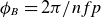
We note that the approximate geometric situation described above is not limited to QI stellarators, since tokamaks with reverse triangularity often exhibit similar double-well behaviour, see figures 15(b) and 15(c) of Balestri et al. (Reference Balestri, Ball, Coda, Cruz-Zabala, Garcia-Munoz and Viezzer2024). We show a toy model geometry in figure 1 which has qualitative elements that can arise in both geometries, in that the drift curvature contains a null (or nearly zero) region of finite width and
 $g^{\alpha \alpha } = |\boldsymbol{\nabla }\alpha |^2$
is amplified over the region of bad curvature as a result of magnetic shear. Negative triangularity tokamaks have apparent ITG stability benefits such as relatively high CGs (Balestri et al. Reference Balestri, Ball, Coda, Cruz-Zabala, Garcia-Munoz and Viezzer2024), an effect which stellarators may emulate, despite belonging to a different geometry class. A CG model capable of handling such cases would thus also allow modelling of more complex stellarator and tokamak cases while avoiding possible issues related to evaluating
$g^{\alpha \alpha } = |\boldsymbol{\nabla }\alpha |^2$
is amplified over the region of bad curvature as a result of magnetic shear. Negative triangularity tokamaks have apparent ITG stability benefits such as relatively high CGs (Balestri et al. Reference Balestri, Ball, Coda, Cruz-Zabala, Garcia-Munoz and Viezzer2024), an effect which stellarators may emulate, despite belonging to a different geometry class. A CG model capable of handling such cases would thus also allow modelling of more complex stellarator and tokamak cases while avoiding possible issues related to evaluating
 $g^{\alpha \alpha }$
at a single point. Furthermore, such a model could be used in optimisation to force the parallel connection length of localised toroidal modes to lie within the now-separated drift wells, effectively doubling the CG (by halving
$g^{\alpha \alpha }$
at a single point. Furthermore, such a model could be used in optimisation to force the parallel connection length of localised toroidal modes to lie within the now-separated drift wells, effectively doubling the CG (by halving
 $L_{\parallel }$
in expression (2.3)). We refer to this as ‘splitting the mode’ (§ 2.4) and now describe how we refine the CG model to handle such cases.
$L_{\parallel }$
in expression (2.3)). We refer to this as ‘splitting the mode’ (§ 2.4) and now describe how we refine the CG model to handle such cases.
Left: simplified toy model geometry for the drift curvature
 $K_{d}$
and squared gradient of the binormal coordinate (
$K_{d}$
and squared gradient of the binormal coordinate (
 $g^{\alpha \alpha } = |\boldsymbol{\nabla } \alpha |^{2}$
) depicted along a magnetic field line (
$g^{\alpha \alpha } = |\boldsymbol{\nabla } \alpha |^{2}$
) depicted along a magnetic field line (
 $\ell$
coordinate), with split drift curvature wells and secularly increasing
$\ell$
coordinate), with split drift curvature wells and secularly increasing
 $g^{\alpha \alpha }$
. A QI stellarator, or reverse triangularity tokamak with large magnetic shear and flat surfaces near the outboard midplane, could qualitatively achieve such geometry profiles. Right: magnetic flux surfaces and outer boundary for a QI configuration at zero toroidal angle as defined in the VMEC code (Hirschman & Whitson Reference Hirshman and Whitson1983) with a ‘reverse-D’ shape at the maximum of
$g^{\alpha \alpha }$
. A QI stellarator, or reverse triangularity tokamak with large magnetic shear and flat surfaces near the outboard midplane, could qualitatively achieve such geometry profiles. Right: magnetic flux surfaces and outer boundary for a QI configuration at zero toroidal angle as defined in the VMEC code (Hirschman & Whitson Reference Hirshman and Whitson1983) with a ‘reverse-D’ shape at the maximum of
 $B$
. Note the relative compression of the surfaces on the outboard. Roughly constant magnetic field (as the poloidal angle is traversed) is achieved by offsetting the
$B$
. Note the relative compression of the surfaces on the outboard. Roughly constant magnetic field (as the poloidal angle is traversed) is achieved by offsetting the
 $1/r$
scaling of
$1/r$
scaling of
 $B$
with surface expansion on the inboard and compression on the outboard.
$B$
with surface expansion on the inboard and compression on the outboard.

2.3. Updated CG model
We now imagine coarse graining of the geometry as a kind of field line average that takes place over a single region of bad curvature in which the sign of the bad curvature does not reverse. We update the previous model (Roberg-Clark et al. Reference Roberg-Clark, Plunk, Xanthopoulos, Nührenberg, Henneberg and Smith2023) by defining the root-mean-squared average
 \begin{equation} \langle (\cdots) \rangle _{CG} (\ell ) = \left [ \frac { \ \int \varTheta (K_{d}(\ell ^{\prime })) (\cdots)^{2}(\ell ^{\prime }) \varTheta _{w}(\ell ,\ell ^{\prime }) {\rm d} \ell ^{\prime } }{ \int \varTheta (K_{d}(\ell ^{\prime })) \varTheta _{w}(\ell ,\ell ^{\prime }) {\rm d} \ell ^{\prime }} \right ]^{1/2}, \end{equation}
to calculate quantities like the average of
 $|\boldsymbol{\nabla } \alpha |$
instead of choosing the central peak fitted value of
$|\boldsymbol{\nabla } \alpha |$
instead of choosing the central peak fitted value of
 $|\boldsymbol{\nabla } \alpha |$
as before. The ‘observation point’
$|\boldsymbol{\nabla } \alpha |$
as before. The ‘observation point’
 $\ell$
effectively sets the mode location, as enforced by the Heaviside function
$\ell$
effectively sets the mode location, as enforced by the Heaviside function
 $\varTheta _{w}(\ell ,\ell ^{\prime })$
, which is
$\varTheta _{w}(\ell ,\ell ^{\prime })$
, which is
 $1$
if
$1$
if
 $K_{d}$
has no sign changes between
$K_{d}$
has no sign changes between
 $\ell$
and
$\ell$
and
 $\ell ^{\prime }$
and zero otherwise. This restricts the integration to single drift wells, where the other Heaviside function,
$\ell ^{\prime }$
and zero otherwise. This restricts the integration to single drift wells, where the other Heaviside function,
 $\varTheta (K_{d}(\ell ^{\prime }))$
, is
$\varTheta (K_{d}(\ell ^{\prime }))$
, is
 $1$
where
$1$
where
 $K_{d}$
is negative (destabilising) and zero otherwise. The parallel connection length is calculated by finding the width of this region, namely
$K_{d}$
is negative (destabilising) and zero otherwise. The parallel connection length is calculated by finding the width of this region, namely
 \begin{equation} L_{\parallel }(\ell )_{CG} = \int \varTheta (K_{d}(\ell ^{\prime })) \varTheta _{w}(\ell ,\ell ^{\prime }) {\rm d} \ell ^{\prime }, \end{equation}
while the average curvature drive at marginal stability is defined as
 \begin{equation} \left ( \frac {a}{R_{\mathrm{eff}}} \right )_{CG}(\ell ) = \frac {1}{L_{\parallel CG}(\ell )} \int K_{d}(\ell ^{\prime }) \varTheta (K_{d}(\ell ^{\prime })) \varTheta _{w}(\ell ,\ell ^{\prime }) {\rm d} \ell ^{\prime }. \end{equation}
Note that, in contrast to the previous model, the integration is carried out such that the endpoints (regions where the sign of
 $K_{d}$
flips between two grid points) are included with linear interpolation in the integral. Armed with more general methods for calculating averages, we express the new CG along a single field line
$K_{d}$
flips between two grid points) are included with linear interpolation in the integral. Armed with more general methods for calculating averages, we express the new CG along a single field line
 $\alpha$
as
$\alpha$
as
 \begin{equation} \frac {a}{L_{T,crit}}(\alpha ) = \text{Min}_{\ell } \left [ \pi \left ( \frac {1+\tau }{2} \right ) \left (3.75 \: \langle a|\boldsymbol{\nabla } \alpha | \rangle _{CG}(\ell ) \frac {a}{L_{\parallel CG}(\ell )} \right ) \right ], \end{equation}
which ignores any explicit dependence on
 $R_{\mathrm{eff}}$
(consistent with the weak curvature limit) and uses a coefficient of half the size compared with the old model for the
$R_{\mathrm{eff}}$
(consistent with the weak curvature limit) and uses a coefficient of half the size compared with the old model for the
 $L_{\parallel }$
term. Implemented as an optimisation target, the method scans over all observation points
$L_{\parallel }$
term. Implemented as an optimisation target, the method scans over all observation points
 $\ell$
present in the given flux tube and finds the location corresponding to the minimum CG. The lack of explicit dependence on
$\ell$
present in the given flux tube and finds the location corresponding to the minimum CG. The lack of explicit dependence on
 $R_{\mathrm{eff}}$
means that during optimisation the size of curvature will be determined by properties other than the CG, like the aspect ratio, number of field periods, imposition of a vacuum magnetic well and addition of plasma
$R_{\mathrm{eff}}$
means that during optimisation the size of curvature will be determined by properties other than the CG, like the aspect ratio, number of field periods, imposition of a vacuum magnetic well and addition of plasma
 $\beta$
, which modifies the drift curvature profile. In this finite
$\beta$
, which modifies the drift curvature profile. In this finite
 $\beta$
limit we use the curvature drift, as defined through
$\beta$
limit we use the curvature drift, as defined through
 $K_{d}$
in § 2.1. The target is then defined as
$K_{d}$
in § 2.1. The target is then defined as
 \begin{align} f_{CG}(r)=\left (\text{Min}_{\alpha }\left [\frac {a}{L_{T,crit}}(\alpha )\right ]-2.0\right )^{2} ,\end{align}
which can be used to improve the CG during optimisation on a specific surface
 $r$
. For all of the cases in this paper, we optimise at
$r$
. For all of the cases in this paper, we optimise at
 $r/a=0.5$
.
$r/a=0.5$
.
2.4. Splitting the mode
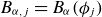
Splitting ITG modes – idealised field line geometry metrics at the typically most unstable location on the outboard midplane of a QI magnetic field configuration. (a) No attempt is made to split the mode geometrically across the standard gap at
 $\ell =0$
. Thus the mode can average the drift curvature across the gap. We surmise that
$\ell =0$
. Thus the mode can average the drift curvature across the gap. We surmise that
 $(a/R_{\mathrm{eff}})_{CG}$
will be similar to a case with no gap. The mode freely ‘tunnels’ across the gap to encompass an
$(a/R_{\mathrm{eff}})_{CG}$
will be similar to a case with no gap. The mode freely ‘tunnels’ across the gap to encompass an
 $L_{\parallel }$
of the entire well (achieving a low CG) with similar curvature drive to modes that localise on each side of the gap. (b) A barrier is imposed by the geometry through
$L_{\parallel }$
of the entire well (achieving a low CG) with similar curvature drive to modes that localise on each side of the gap. (b) A barrier is imposed by the geometry through
 $g^{\alpha \alpha } = |\boldsymbol{\nabla }\alpha |^2$
, reducing the growth rate of the mode that tunnels across the gap. (c) Separating the two wells reduces the average curvature drive significantly for the tunnelling mode, as similarly portrayed in figure 1. Additional shear amplification of
$g^{\alpha \alpha } = |\boldsymbol{\nabla }\alpha |^2$
, reducing the growth rate of the mode that tunnels across the gap. (c) Separating the two wells reduces the average curvature drive significantly for the tunnelling mode, as similarly portrayed in figure 1. Additional shear amplification of
 $g^{\alpha \alpha }$
further stabilises the localised modes.
$g^{\alpha \alpha }$
further stabilises the localised modes.

Having found a CG formula that is compatible with well splitting, we can discuss how this effect is realised in practice. In particular, we imagine two different ways to ensure that the parallel connection length of toroidal ITG modes is halved by splitting the mode. The goal here, via manipulating the field line geometry, is to decouple the behaviour of modes that straddle both wells and those that localise to individual wells. The localised modes should then be further stabilised by the geometry.
To illustrate the common (un-optimised) situation for QI stellarators, we first show a case where no attempt is made to split the mode, aside from having a zero point of curvature (figure 2 a). In this case the mode can simply ‘tunnel’ across the gap at little cost to the average value of the curvature (the gap is small compared with the overall width of the region). The end result is a mode with a parallel connection length containing both drift wells that is not significantly affected, in terms of curvature drive or parallel dynamics, by a null point in the curvature.
A way to more effectively split the mode was already shown in figure 1 – to make the gap between the two resulting wells large, such that the gap is comparable to or larger than the width of the two wells, as also shown in figure 2(c). The modes which are strongly driven by curvature will be forced to localise in each separate well, and their stability will then be set by the local drift well behaviour, while the mode that spreads across the barrier will experience a reduced curvature drive
 $(a/R_{\mathrm{eff}})_{CG}$
as long as the curvature does not increase in proportion to the widening of the gap. Note this means that residual turbulence may grow at a CG below that of the more localised modes, since they have a larger
$(a/R_{\mathrm{eff}})_{CG}$
as long as the curvature does not increase in proportion to the widening of the gap. Note this means that residual turbulence may grow at a CG below that of the more localised modes, since they have a larger
 $L_{\parallel }$
, which we believe will produce a ‘foot’ in plots of nonlinear heat flux versus temperature gradient (Zocco et al. Reference Zocco, Xanthopoulos, Doerk, Connor and Helander2018, Reference Zocco, Podavini, Garcìa-Regaña, Barnes, Parra and Mishchenko2022). A second way to split the well is to insert a barrier through which ITG modes with strong curvature drive cannot tunnel, in this case by increasing
$L_{\parallel }$
, which we believe will produce a ‘foot’ in plots of nonlinear heat flux versus temperature gradient (Zocco et al. Reference Zocco, Xanthopoulos, Doerk, Connor and Helander2018, Reference Zocco, Podavini, Garcìa-Regaña, Barnes, Parra and Mishchenko2022). A second way to split the well is to insert a barrier through which ITG modes with strong curvature drive cannot tunnel, in this case by increasing
 $\boldsymbol{\nabla } \alpha$
at the central location
$\boldsymbol{\nabla } \alpha$
at the central location
 $\ell =0$
on the flux tube (Roberg-Clark, Plunk & Xanthopoulos Reference Roberg-Clark, Plunk and Xanthopoulos2021) (figure 2
b). The mode that tunnels suffers reduced growth rates as a result. We show stellarator configurations which utilise the first method later in the paper.
$\ell =0$
on the flux tube (Roberg-Clark, Plunk & Xanthopoulos Reference Roberg-Clark, Plunk and Xanthopoulos2021) (figure 2
b). The mode that tunnels suffers reduced growth rates as a result. We show stellarator configurations which utilise the first method later in the paper.
As already mentioned, the mode splitting (starting with a null point in the drift curvature), if it is present or nearly occurring in a vacuum magnetic equilibrium, can be altered by the shift in the curvature drift in the gyrokinetic equation brought about by a finite
 $\beta$
term proportional to
$\beta$
term proportional to
 $\boldsymbol{\nabla } p / B^{2}$
. This term can make bad curvature worse since on the outboard the temperature gradient and normal curvature vectors tend to be parallel. As such, the curvature drift may capture a lower CG from an increase in
$\boldsymbol{\nabla } p / B^{2}$
. This term can make bad curvature worse since on the outboard the temperature gradient and normal curvature vectors tend to be parallel. As such, the curvature drift may capture a lower CG from an increase in
 $L_{\parallel CG}$
in finite
$L_{\parallel CG}$
in finite
 $\beta$
systems.
$\beta$
systems.
2.5. Ion-temperature-gradient instability above the threshold
Once the ITG modes are localised to individual drift wells, it remains to be seen how stable they will be. Growth rates for these modes depend on a variety of geometric factors, such as the magnitudes of
 $K_{d}$
,
$K_{d}$
,
 $|\boldsymbol{\nabla } \alpha |$
and
$|\boldsymbol{\nabla } \alpha |$
and
 $|\boldsymbol{\nabla } \psi |$
. Since, above the threshold, modes continue to localise in regions of bad curvature, we slightly modify the average in (2.4) by weighting it with the magnitude of curvature
$|\boldsymbol{\nabla } \psi |$
. Since, above the threshold, modes continue to localise in regions of bad curvature, we slightly modify the average in (2.4) by weighting it with the magnitude of curvature
 \begin{equation} \langle (\boldsymbol{\cdot }\boldsymbol{\cdot }\boldsymbol{\cdot }) \rangle _d (\ell ) = \left [ \frac { \int \: K_{d}(\ell ^{\prime }) \varTheta (K_{d}(\ell ^{\prime })) (\boldsymbol{\cdot }\boldsymbol{\cdot }\boldsymbol{\cdot })^{2}(\ell ^{\prime }) \varTheta _{w}(\ell ,\ell ^{\prime }){\rm d} \ell ^{\prime }}{\int K_{d}(\ell ^{\prime }) \varTheta (K_{d}(\ell ^{\prime }))\varTheta _{w}(\ell ,\ell ^{\prime }) {\rm d} \ell ^{\prime }} \right ]^{1/2} . \end{equation}
This factor will take into account surface compression (through relating
 $\boldsymbol{\nabla } \psi$
to
$\boldsymbol{\nabla } \psi$
to
 $\boldsymbol{\nabla } \alpha$
through
$\boldsymbol{\nabla } \alpha$
through
 $\boldsymbol{B}$
) and local and global shear effects that stabilise the localised ITG modes above the CG.
$\boldsymbol{B}$
) and local and global shear effects that stabilise the localised ITG modes above the CG.
2.6. Kinetic electrons
An additional factor is the effect of kinetic electrons on ITG mode growth rates. The non-adiabatic response of electrons can significantly increase growth rates and nonlinear heat fluxes of ITG modes compared with the adiabatic electron case (see e.g. Proll et al. Reference Proll, Plunk, Faber, Görler, Helander, McKinney, Pueschel, Smith and Xanthopoulos2022). Several strategies to combat this enhanced drive from trapped particles have been developed in recent years with regards to trapped electron modes, including calculations of the available energy for turbulence (Mackenbach et al. Reference Mackenbach, Proll and Helander2022, Reference Mackenbach, Proll, Wakelkamp and Helander2023; Duff et al. Reference Duff, Faber, Hegna, Pueschel and Terry2025), modifying flux surface shaping in both tokamaks (Garbet et al. Reference Garbet, Donnel, Gianni, Qu, Melka, Sarazin, Grandgirard, Obrejan, Bourne and Dif-Pradalier2024) and stellarators (Gerard et al. Reference Gerard, Pueschel, Geiger, Mackenbach, Duff, Faber, Hegna and Terry2024) or directly targeting the overlap of trapped particles with drift curvature (Proll et al. Reference Proll, Mynick, Xanthopoulos, Lazerson and Faber2016; Gerard et al. Reference Gerard, Geiger, Pueschel, Bader, Hegna, Faber, Terry, Kumar and Schmitt2023). Recent theoretical work (Costello & Plunk, 2025a) focused on the modification of linear, toroidal ITG mode growth rates
 \begin{align} \omega = \pm \sqrt{-{\omega_{*i}}\int_{-\infty}^{\infty}\frac{d\ell}{B} \hat{\omega}_{di}(\ell)|\delta \phi|^{2} }\left( \tau \int_{-\infty}^{+\infty}|\delta \phi |^{2} \frac{dl}{B} - \frac{\tau}{2} \Sigma_{j} \int_{{1}/{B_{min}}}^{{1}/{B_{max}}} \tau_{B,j} |\overline{\delta \phi_{j}}|^{2} d\lambda\! \right)^{-({1}/{2})}\!, \end{align}
where the bounce average is
 \begin{equation} \overline {(\boldsymbol{\cdot }\boldsymbol{\cdot }\boldsymbol{\cdot })} = \frac {1}{\tau _{b}}\int ^{\ell _{2}}_{\ell _{1}} \frac {(\boldsymbol{\cdot }\boldsymbol{\cdot }\boldsymbol{\cdot })}{\sqrt {1-\lambda B}} {\rm d}\ell ,\end{equation}
and the bounce time is
 $\tau_{B} = \int^{{\ell}_{2}}_{{\ell}_{1}} (1-\lambda B)^{-({1}/{2})} d\ell$
. Several effects are at play in (2.10). The first is the integral along the field line of the drift curvature
$\tau_{B} = \int^{{\ell}_{2}}_{{\ell}_{1}} (1-\lambda B)^{-({1}/{2})} d\ell$
. Several effects are at play in (2.10). The first is the integral along the field line of the drift curvature
 $\hat {\omega }_{di}(\ell ) \propto -K_{d}(\ell )$
, indicating stability based on the size and sign of the average curvature. Negative curvature in this notation indicates stability of the mode, and is a motivating factor for the max-J property (Proll et al. Reference Proll, Helander, Connor and Plunk2012; Rodríguez et al. Reference Rodríguez, Helander and Goodman2024) where J is the parallel adiabatic invariant of particles, and max-J refers to the case where J is a decreasing function of radius, which has led to successful QI designs with reduced turbulence (Goodman et al. Reference Goodman, Xanthopoulos, Plunk, Smith, Nührenberg, Beidler, Henneberg, Roberg-Clark, Drevlak and Helander2024; García-Regaña et al. Reference García-Regaña, Calvo, Sánchez, Thienpondt, Velasco and Capitán2025). The ITG modes can be completely stabilised in cases where the mode extent includes both regions of good and bad curvature, since the average over this region can be of the ‘good’ sign (figure 3
a). However, toroidal magnetic fields must have some regions of bad curvature, and we are exploring ITG modes that only exist in regions of bad curvature. The max-J property itself cannot stabilise such modes, since
$\hat {\omega }_{di}(\ell ) \propto -K_{d}(\ell )$
, indicating stability based on the size and sign of the average curvature. Negative curvature in this notation indicates stability of the mode, and is a motivating factor for the max-J property (Proll et al. Reference Proll, Helander, Connor and Plunk2012; Rodríguez et al. Reference Rodríguez, Helander and Goodman2024) where J is the parallel adiabatic invariant of particles, and max-J refers to the case where J is a decreasing function of radius, which has led to successful QI designs with reduced turbulence (Goodman et al. Reference Goodman, Xanthopoulos, Plunk, Smith, Nührenberg, Beidler, Henneberg, Roberg-Clark, Drevlak and Helander2024; García-Regaña et al. Reference García-Regaña, Calvo, Sánchez, Thienpondt, Velasco and Capitán2025). The ITG modes can be completely stabilised in cases where the mode extent includes both regions of good and bad curvature, since the average over this region can be of the ‘good’ sign (figure 3
a). However, toroidal magnetic fields must have some regions of bad curvature, and we are exploring ITG modes that only exist in regions of bad curvature. The max-J property itself cannot stabilise such modes, since
 $|\delta \phi | =0$
in regions of good curvature, by definition (see figure 3
b). Thus the average drive of these modes will be unaffected by the max-J property once they are driven unstable above the CG.
$|\delta \phi | =0$
in regions of good curvature, by definition (see figure 3
b). Thus the average drive of these modes will be unaffected by the max-J property once they are driven unstable above the CG.
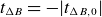
Inverse mirror configurations sidestep mode inertia – idealised schematics for different QI magnetic field shapes along a magnetic field line with different, roughly constant ITG mode potentials but the same QI-like curvature profile
 $K_{d}$
. (a) A standard broad minimum and narrow maximum which leverages the max-J property. The spread-out mode potential achieves no net curvature drive and is stable. (b) The same geometry but with sufficient drive such that the CG for a localised ITG mode is exceeded, which sits only in the bad curvature well. The mode inertia effect now increases drive for the ITG mode roughly by the factor
$K_{d}$
. (a) A standard broad minimum and narrow maximum which leverages the max-J property. The spread-out mode potential achieves no net curvature drive and is stable. (b) The same geometry but with sufficient drive such that the CG for a localised ITG mode is exceeded, which sits only in the bad curvature well. The mode inertia effect now increases drive for the ITG mode roughly by the factor
 $(1-\sqrt {1-B_{\text{min}}/B_{\text{max}}} )^{-1}$
. (c) An ‘inverse mirror’ (IM) magnetic field with a narrow minimum and broad maximum avoids the mode inertia effect by removing trapped particles from the bad curvature region (
$(1-\sqrt {1-B_{\text{min}}/B_{\text{max}}} )^{-1}$
. (c) An ‘inverse mirror’ (IM) magnetic field with a narrow minimum and broad maximum avoids the mode inertia effect by removing trapped particles from the bad curvature region (
 $\langle \epsilon (\ell ) \rangle \rightarrow 0$
).
$\langle \epsilon (\ell ) \rangle \rightarrow 0$
).

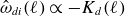
To reduce the growth rates of localised ITG modes in the kinetic electron regime, we are left with the options of reducing the magnitude of the bad curvature in the numerator or reducing the effect of non-adiabatic electrons in the denominator. As already stated, we would prefer to leave the former quantity alone during optimisation. The latter effect was referred to as ‘mode inertia’ (Costello & Plunk, Reference Costello and Plunk2025a
) and results from the presence of trapped particles capable of strongly destabilising ITG modes. Note that, in the limit of a square well magnetic field, for which
 $B=B_{\min}$
in some central region bounded by step functions with height
$B=B_{\min}$
in some central region bounded by step functions with height
 $B=B_{\max}$
, the second term in the denominator includes the trapped particle fraction
$B=B_{\max}$
, the second term in the denominator includes the trapped particle fraction
 $\epsilon = \sqrt {1-B_{\min}/B_{\max}}$
. Since the overall denominator is positive–definite, it reduces in magnitude from the non-adiabatic response and leads to increased growth rates. To make an estimate for spatially varying magnetic fields with ITG modes localised to regions of bad curvature, we carry out the
$\epsilon = \sqrt {1-B_{\min}/B_{\max}}$
. Since the overall denominator is positive–definite, it reduces in magnitude from the non-adiabatic response and leads to increased growth rates. To make an estimate for spatially varying magnetic fields with ITG modes localised to regions of bad curvature, we carry out the
 $\lambda$
integration in the second term of the denominator. To evaluate the factor
$\lambda$
integration in the second term of the denominator. To evaluate the factor
 $|\overline {\delta \phi }|^{2}$
, which is the modulus squared of the bounce-averaged potential, we use the Cauchy–Schwarz inequality
$|\overline {\delta \phi }|^{2}$
, which is the modulus squared of the bounce-averaged potential, we use the Cauchy–Schwarz inequality
 \begin{equation} |\overline {\delta \phi }|^{2} \leqslant \overline {|\delta \phi |^{2}} \end{equation}
(Helander, Proll & Plunk Reference Helander, Proll and Plunk2013) for which the equality holds in the case of a constant potential. In fact, the case of equality is an upper bound on the destabilising effect of the denominator, so we can use it to estimate the strongest effect of trapped electrons on the mode growth. Assuming a constant potential but this time in the bad curvature region and doing the
 $\lambda$
integration over the region of finite potential
$\lambda$
integration over the region of finite potential
 $\delta \phi$
, we find the field line average of
$\delta \phi$
, we find the field line average of
 $\delta \phi$
squared over B with a spatially varying trapped particle fraction
$\delta \phi$
squared over B with a spatially varying trapped particle fraction
 $\epsilon (\ell ) = \sqrt {1-B(\ell )/B_{\max}}$
, where contributions to the integral outside of the bad curvature region are ignored. Note that this is equivalent to using a trial function for the potential which is a step function located entirely in the bad curvature region. The result is
$\epsilon (\ell ) = \sqrt {1-B(\ell )/B_{\max}}$
, where contributions to the integral outside of the bad curvature region are ignored. Note that this is equivalent to using a trial function for the potential which is a step function located entirely in the bad curvature region. The result is
 \begin{align} \omega = \pm \sqrt {-\omega _{*i} \langle \hat {\omega }_{di} \rangle _{\delta \phi }/ \langle (1-\epsilon (\ell ) \rangle _{\delta \phi } }, \end{align}
where, as in Costello & Plunk (Reference Costello and Plunk2025a ), the volume average including the mode potential is
 \begin{align} \langle (\boldsymbol{\cdot }\boldsymbol{\cdot }\boldsymbol{\cdot }) \rangle _{\delta \phi } = \int _{-\infty }^{\infty } (\boldsymbol{\cdot }\boldsymbol{\cdot }\boldsymbol{\cdot }) |\delta \phi |^{2} \frac {{\rm d} \ell }{B}. \end{align}
For the purposes of optimisation, we can approximate this average with the definition
 $\langle (\boldsymbol{\cdot }\boldsymbol{\cdot }\boldsymbol{\cdot })\rangle _d$
used in (2.9), since this estimates the effect of mode localisation in the region of peak bad curvature. In doing so we ignore the factor
$\langle (\boldsymbol{\cdot }\boldsymbol{\cdot }\boldsymbol{\cdot })\rangle _d$
used in (2.9), since this estimates the effect of mode localisation in the region of peak bad curvature. In doing so we ignore the factor
 $1/B$
in the
$1/B$
in the
 $\ell$
integrals in both the numerator and denominator for simplicity.
$\ell$
integrals in both the numerator and denominator for simplicity.
Expression (2.13) suggests that we can shift trapped particles to a region of zero or good curvature in order to increase mode inertia (i.e. stabilise the mode), in line with work such as Proll et al. (Reference Proll, Mynick, Xanthopoulos, Lazerson and Faber2016) and Gerard et al. (Reference Gerard, Geiger, Pueschel, Bader, Hegna, Faber, Terry, Kumar and Schmitt2023). An idealised example of this would be the limit of a very narrow square well magnetic field where for the most part
 $B=B_{\max}$
with a small region of
$B=B_{\max}$
with a small region of
 $B=B_{\min}$
, in which the curvature is either zero or stabilising. Such magnetic fields can be achieved by optimising QI configurations to have an IM shape as shown in figure 3(c). Modern optimisation of QI designs (Subbotin et al. Reference Subbotin2006; Sánchez et al. Reference Sánchez, Velasco, Calvo and Mulas2023; Goodman et al. Reference Goodman, Xanthopoulos, Plunk, Smith, Nührenberg, Beidler, Henneberg, Roberg-Clark, Drevlak and Helander2024) has tended to lead towards configurations with a broad, flat magnetic field minimum that traps a large number of particles in a region of small field line curvature. The magnetic field around the corresponding minimum of
$B=B_{\min}$
, in which the curvature is either zero or stabilising. Such magnetic fields can be achieved by optimising QI configurations to have an IM shape as shown in figure 3(c). Modern optimisation of QI designs (Subbotin et al. Reference Subbotin2006; Sánchez et al. Reference Sánchez, Velasco, Calvo and Mulas2023; Goodman et al. Reference Goodman, Xanthopoulos, Plunk, Smith, Nührenberg, Beidler, Henneberg, Roberg-Clark, Drevlak and Helander2024) has tended to lead towards configurations with a broad, flat magnetic field minimum that traps a large number of particles in a region of small field line curvature. The magnetic field around the corresponding minimum of
 $B$
tends to be relatively straight and wide in real space while the maximum of
$B$
tends to be relatively straight and wide in real space while the maximum of
 $B$
tends to be narrow and exhibit bean-shaped cross-sections reminiscent of that seen in Wendelstein 7-X configurations. However, the IM magnetic field is another possible solution of the near-axis equations in QI geometry. While this type of configuration may struggle to fulfil the max-J property, it nonetheless has the tendency to push bad curvature close to the maximum of
$B$
tends to be narrow and exhibit bean-shaped cross-sections reminiscent of that seen in Wendelstein 7-X configurations. However, the IM magnetic field is another possible solution of the near-axis equations in QI geometry. While this type of configuration may struggle to fulfil the max-J property, it nonetheless has the tendency to push bad curvature close to the maximum of
 $B$
such that
$B$
such that
 $\langle \epsilon (\ell ) \rangle \rightarrow 0$
. In this limit it may be possible to achieve similar levels of ITG stability without enforcing the maximum J property, as we shall later see. We emphasise that it is not required for a magnetic field to be in this extreme limit to achieve reasonable stabilisation, merely that it is one way to stabilise ITG modes via expression (2.13) at finite mirror ratio.
$\langle \epsilon (\ell ) \rangle \rightarrow 0$
. In this limit it may be possible to achieve similar levels of ITG stability without enforcing the maximum J property, as we shall later see. We emphasise that it is not required for a magnetic field to be in this extreme limit to achieve reasonable stabilisation, merely that it is one way to stabilise ITG modes via expression (2.13) at finite mirror ratio.
3. Omnigeneity targets
Here, we discuss the general optimisation strategy employed in the paper to achieve better ITG stability in QI configurations. We target omnigeneity, the property of zero bounce-averaged radial particle drifts, with poloidally closing contours of magnetic field strength. In practice, the resulting configurations are approximately QI, but with poloidally straight contours near the minimum of the magnetic field. This behaviour results because we prescribe fixed toroidal angles for the minimum and maximum of the magnetic field strength in Boozer coordinates, but at locations away from the extrema the field contours are allowed to ‘wobble’ in the Boozer plane with excursions in the poloidal and toroidal directions, in typical QI fashion. On every magnetic field line, using now
 $\phi _{B}$
as the field-line-following coordinate, we ask that the magnetic field achieves its maximum at the locations
$\phi _{B}$
as the field-line-following coordinate, we ask that the magnetic field achieves its maximum at the locations
 $\phi _{B}=0$
and
$\phi _{B}=0$
and
 $\phi _{B}=2\pi /nfp$
, and its minimum at the locations
$\phi _{B}=2\pi /nfp$
, and its minimum at the locations
 $\phi _{B}=\pi /n_{fp}$
, with
$\phi _{B}=\pi /n_{fp}$
, with
 $n_{fp}$
the number of field periods and
$n_{fp}$
the number of field periods and
 $\phi _{B}$
the toroidal Boozer angle (Boozer Reference Boozer1981). We also ask that the magnetic field strength
$\phi _{B}$
the toroidal Boozer angle (Boozer Reference Boozer1981). We also ask that the magnetic field strength
 $B$
decreases (increases) monotonically from the field maximum (minimum) to the minimum (maximum) on every field line, penalising cases where the derivative
$B$
decreases (increases) monotonically from the field maximum (minimum) to the minimum (maximum) on every field line, penalising cases where the derivative
 $B^{\prime }(\ell )$
lies below or above a target value, depending on whether the point is on the left or right side of the
$B^{\prime }(\ell )$
lies below or above a target value, depending on whether the point is on the left or right side of the
 $B$
well. We target a mirror ratio near the magnetic axis of
$B$
well. We target a mirror ratio near the magnetic axis of
 $25\,\%$
 \begin{equation} f_{mirror} = ((B_{\max}-B_{\min})/(B_{\max}+B_{\min}) - 0.25)^{2} ,\end{equation}
with
 $B_{\max}$
the global maximum and
$B_{\max}$
the global maximum and
 $B_{\min}$
the global minimum on the surface, while the target for the maxima and minima is
$B_{\min}$
the global minimum on the surface, while the target for the maxima and minima is
 \begin{equation} f_{\text{extrema}} = \sum _{\alpha } \left [ (B_{\alpha }(\phi _{B}=0)-\text{max}[B_{i}(\phi _{B})])^{2} + (B_{\alpha }(\phi _{B}=\pi /n_{fp})-\text{min}[B_{\alpha }(\phi _{B})])^{2} \right ] ,\end{equation}
where
 $B_{\alpha }(\phi _{B})$
is the field line dependence of the magnetic field strength for the field line label
$B_{\alpha }(\phi _{B})$
is the field line dependence of the magnetic field strength for the field line label
 $\alpha$
. Finally, the monotonicity target, which sums over all locations
$\alpha$
. Finally, the monotonicity target, which sums over all locations
 $\phi _{j}$
for the field line label
$\phi _{j}$
for the field line label
 $\alpha$
and evaluates
$\alpha$
and evaluates
 $B_{\alpha ,j}=B_{\alpha }(\phi _{j})$
, reads
$B_{\alpha ,j}=B_{\alpha }(\phi _{j})$
, reads
 \begin{equation} f_{\text{mono}} = \sum _{\alpha ,j} \varTheta _{\Delta B}((B_{\alpha ,j+1}-B_{\alpha ,j})-t_{\Delta B})((B_{\alpha ,j+1}-B_{\alpha ,j}) - t_{\Delta B})^{2} ,\end{equation}
where to the left of the actual minimum of
 $B_{\alpha }$
the desired floor on the change in
$B_{\alpha }$
the desired floor on the change in
 $B$
is
$B$
is
 $t_{\Delta B}=-|t_{\Delta B,0}|$
and to the right of it,
$t_{\Delta B}=-|t_{\Delta B,0}|$
and to the right of it,
 $t_{\Delta B}=|t_{\Delta B,0}|$
, with
$t_{\Delta B}=|t_{\Delta B,0}|$
, with
 $t_{\Delta B,0}$
usually a small value close to
$t_{\Delta B,0}$
usually a small value close to
 $10^{-3}$
for
$10^{-3}$
for
 $128$
points in
$128$
points in
 $\phi$
. Here,
$\phi$
. Here,
 $\varTheta _{\Delta B}$
is the Heaviside step function. This target not only enforces monotonicity but also tries to remove numerically difficult points where
$\varTheta _{\Delta B}$
is the Heaviside step function. This target not only enforces monotonicity but also tries to remove numerically difficult points where
 $\partial {B}/\partial {\phi _{B}}$
is zero identically.
$\partial {B}/\partial {\phi _{B}}$
is zero identically.
3.1. Small orbit widths
It has been argued by Plunk & Helander (Reference Plunk and Helander2024) and shown via optimisation (Goodman et al. Reference Goodman, Xanthopoulos, Plunk, Smith, Nührenberg, Beidler, Henneberg, Roberg-Clark, Drevlak and Helander2024) that QI configurations with low neoclassical transport tend to have robust zonal flow suppression of turbulence. Theoretically, it was argued that this effect comes from the small orbit width of particles in QI fields (compared with tokamaks or quasisymmetric stellarators), related to the relatively small distance between particle bounce points. By choosing QI configurations as candidates for turbulence optimisation, we seek to leverage this property in addition to the CG and growth rate strategies discussed earlier. Having an additional contour at the minimum of
 $B$
be poloidally straight (i.e. a contour of constant
$B$
be poloidally straight (i.e. a contour of constant
 $\phi _{B}$
) in the Boozer plane also seems advantageous from this perspective. This forces the magnetic surface to achieve low geodesic curvature as the poloidal derivative of
$\phi _{B}$
) in the Boozer plane also seems advantageous from this perspective. This forces the magnetic surface to achieve low geodesic curvature as the poloidal derivative of
 $B$
is small in the vicinity of
$B$
is small in the vicinity of
 $B_{\text{min}}$
. Small geodesic curvature has been known to be favourable for zonal flow reduction of electrostatic turbulence (Nunami, Watanabe & Sugama Reference Nunami, Watanabe and Sugama2013; Nakata & Matsuoka Reference Nakata and Matsuoka2022; Nishimoto et al. Reference Nishimoto2024), tied to the damping of geodesic acoustic modes, and the following results suggest this approach indeed works.
$B_{\text{min}}$
. Small geodesic curvature has been known to be favourable for zonal flow reduction of electrostatic turbulence (Nunami, Watanabe & Sugama Reference Nunami, Watanabe and Sugama2013; Nakata & Matsuoka Reference Nakata and Matsuoka2022; Nishimoto et al. Reference Nishimoto2024), tied to the damping of geodesic acoustic modes, and the following results suggest this approach indeed works.
Since targeting the minimum of
 $B$
to lie at constant toroidal angle seems distinct from previous QI optimisations, we would like to classify it differently. To delineate this case, we define an ‘I-number’ (I as in isodynamic) counting the number of poloidally straight contours, which is
$B$
to lie at constant toroidal angle seems distinct from previous QI optimisations, we would like to classify it differently. To delineate this case, we define an ‘I-number’ (I as in isodynamic) counting the number of poloidally straight contours, which is
 $I=1$
in the case of a standard QI stellarator (one contour at
$I=1$
in the case of a standard QI stellarator (one contour at
 $B_{\text{max}}$
) and
$B_{\text{max}}$
) and
 $I = 2$
approximately in the case of the new optimised configurations presented here (an additional contour at
$I = 2$
approximately in the case of the new optimised configurations presented here (an additional contour at
 $B_{\text{min}}$
). Note that quasi-isodynamicity (Cary & Shasharina Reference Cary and Shasharina1997; Plunk et al. Reference Plunk2019) requires poloidally straight contours to come in pairs (
$B_{\text{min}}$
). Note that quasi-isodynamicity (Cary & Shasharina Reference Cary and Shasharina1997; Plunk et al. Reference Plunk2019) requires poloidally straight contours to come in pairs (
 $\phi = \phi _{\text{min}} \pm \phi _{\text{str}}$
) if they are not located at the minimum, with
$\phi = \phi _{\text{min}} \pm \phi _{\text{str}}$
) if they are not located at the minimum, with
 $\phi _{\min}$
the location of the minimum of
$\phi _{\min}$
the location of the minimum of
 $B$
. Omnigenous magnetic fields with no poloidally straight contours such as piecewise omnigenous configurations (Velasco et al. Reference Velasco, Calvo, Escoto, Sánchez, Thienpondt and Parra2024), the various configurations of Wendelstein 7-X, tokamaks, or quasisymmetric stellarators have
$B$
. Omnigenous magnetic fields with no poloidally straight contours such as piecewise omnigenous configurations (Velasco et al. Reference Velasco, Calvo, Escoto, Sánchez, Thienpondt and Parra2024), the various configurations of Wendelstein 7-X, tokamaks, or quasisymmetric stellarators have
 $I=0$
.
$I=0$
.
3.2. Radial drift
The primary omnigeneity target minimises a version of the quantity
 $\epsilon _{\text{eff}}$
(Nemov et al. Reference Nemov, Kasilov, Kernbichler and Heyn1999) to reduce the net radial drift of particles in accordance with omnigeneity. Instead of taking an average over a very long distance of a single field line (in the limit of the distance
$\epsilon _{\text{eff}}$
(Nemov et al. Reference Nemov, Kasilov, Kernbichler and Heyn1999) to reduce the net radial drift of particles in accordance with omnigeneity. Instead of taking an average over a very long distance of a single field line (in the limit of the distance
 $s$
going to infinity), we sample a large number of field lines ranging from
$s$
going to infinity), we sample a large number of field lines ranging from
 $\phi =0$
to
$\phi =0$
to
 $\phi =2\pi /n_{fp}$
and assume that, over each field period, a single well in the magnetic field exists, such that additional bounce wells are not taken into the calculation. This is enforced with targets (3.3) and (3.2). The target reads
$\phi =2\pi /n_{fp}$
and assume that, over each field period, a single well in the magnetic field exists, such that additional bounce wells are not taken into the calculation. This is enforced with targets (3.3) and (3.2). The target reads
 \begin{align} f_{\overline {\epsilon }_{\text{eff}}} & = \sum _{s_{0}} \overline {\epsilon }_{\text{eff}}^{2}(s_{0}) \nonumber\\[-5pt] \overline {\epsilon }_{\text{eff}}^{3/2} & = \pi R_{0}^{2}\left ( \sum _{\alpha } \int _{\ell _{-}(\alpha )}^{\ell _{+}(\alpha )}\frac {{\rm d}\ell }{B} \right )\left ( \sum _{\alpha } \int _{\ell _{-}(\alpha )}^{\ell _{+}(\alpha )} \boldsymbol{\nabla } \psi \frac {{\rm d}\ell }{B}\right )^{-2}\sum _{\alpha } \int ^{B_{\max}(\alpha )}_{B_{\min}(\alpha )}db^{\prime } \varTheta _{B}(b^{\prime }-B) \frac {\hat {H}^{2}}{\hat {I}} \nonumber \\[5pt] \hat {H}& = \frac {1}{b^{\prime }}\int _{\ell _{-}(\alpha )}^{\ell _{+}(\alpha )}\sqrt {b^{\prime }-\frac {B}{B_{0}}}\left (4\frac {B_{0}}{B}-\frac {1}{b^{\prime }}\right )\boldsymbol{\nabla } \psi \kappa _{g} \frac {{\rm d}\ell }{B} \nonumber \\[5pt] \hat {I} & = \int _{\ell _{-}(\alpha )}^{\ell _{+}(\alpha )}\sqrt {1-\frac {B}{B_{0} b^{\prime }}}\frac {{\rm d}\ell }{B}, \end{align}
with
 $R_{0}$
a fixed major radius used to stop the optimiser from reducing the aspect ratio by deflating the magnitude of
$R_{0}$
a fixed major radius used to stop the optimiser from reducing the aspect ratio by deflating the magnitude of
 $\epsilon _{\text{eff}}$
,
$\epsilon _{\text{eff}}$
,
 $b^{\prime }=B/B_{0}$
measures a specific value of B lying between the local
$b^{\prime }=B/B_{0}$
measures a specific value of B lying between the local
 $B_{\min}$
and
$B_{\min}$
and
 $B_{\max}$
for a specified field line label
$B_{\max}$
for a specified field line label
 $\alpha$
, which contains the toroidal interval
$\alpha$
, which contains the toroidal interval
 $\{0,2\pi \}$
in PEST coordinates (for which the toroidal angle is the standard cylindrical angle, and the poloidal angle is defined to make the field lines straight), while
$\{0,2\pi \}$
in PEST coordinates (for which the toroidal angle is the standard cylindrical angle, and the poloidal angle is defined to make the field lines straight), while
 $B_{0}$
is a reference value of
$B_{0}$
is a reference value of
 $B$
. The step function
$B$
. The step function
 $\varTheta _{B}$
is
$\varTheta _{B}$
is
 $1$
when
$1$
when
 $b^{\prime } \geqslant B$
and zero otherwise.
$b^{\prime } \geqslant B$
and zero otherwise.
4. Optimisation
Results from using the simsopt optimisation framework (Landreman et al. Reference Landreman, Medasani, Wechsung, Giuliani, Jorge and Zhu2021) are summarised in figures 4, 5 and 6, comparing two six-field-period optimised QI configurations (
 $I=2$
, with straight minima and maxima of
$I=2$
, with straight minima and maxima of
 $B$
) with the high mirror (HM) W7-X configuration (
$B$
) with the high mirror (HM) W7-X configuration (
 $I=0$
, with no poloidally straight contours). Figure 5 shows the results of nonlinear flux tube gyrokinetic simulations using the GENE code (Jenko et al. Reference Jenko, Dorland, Kotschenreuther and Rogers2000), scanning in temperature gradient, while figure 6 shows various relevant quantities, such as the rotational transform, vacuum magnetic well and neoclassical transport coefficients, as well as profiles of geodesic curvature along a magnetic field line. Flux tube metrics for gyrokinetic simulations are shown in figure 7, with discussion of the different behaviours for each configuration in the caption. We see in figure 5 that a simple fit of the heat flux in each case to a line, using the data at large gradients
$I=0$
, with no poloidally straight contours). Figure 5 shows the results of nonlinear flux tube gyrokinetic simulations using the GENE code (Jenko et al. Reference Jenko, Dorland, Kotschenreuther and Rogers2000), scanning in temperature gradient, while figure 6 shows various relevant quantities, such as the rotational transform, vacuum magnetic well and neoclassical transport coefficients, as well as profiles of geodesic curvature along a magnetic field line. Flux tube metrics for gyrokinetic simulations are shown in figure 7, with discussion of the different behaviours for each configuration in the caption. We see in figure 5 that a simple fit of the heat flux in each case to a line, using the data at large gradients
 $a/L_{T}$
, can be extrapolated to zero heat flux at locations which are quite close to the model predictions from (2.7). We believe this is because the effects of Landau damping and
$a/L_{T}$
, can be extrapolated to zero heat flux at locations which are quite close to the model predictions from (2.7). We believe this is because the effects of Landau damping and
 $\boldsymbol{\nabla } \alpha$
– the dominant stabilising mechanisms near marginality for localised modes – are more or less accurately modelled by the CG formula (Roberg-Clark et al. Reference Roberg-Clark, Plunk, Xanthopoulos, Nührenberg, Henneberg and Smith2023). If we then assume that the unstable mode with this CG sets the slope
$\boldsymbol{\nabla } \alpha$
– the dominant stabilising mechanisms near marginality for localised modes – are more or less accurately modelled by the CG formula (Roberg-Clark et al. Reference Roberg-Clark, Plunk, Xanthopoulos, Nührenberg, Henneberg and Smith2023). If we then assume that the unstable mode with this CG sets the slope
 $\partial Q / \partial (a/L_{T})$
, the linear fit to
$\partial Q / \partial (a/L_{T})$
, the linear fit to
 $Q$
(see e.g. Nies Reference Nies, Parra, Barnes, Mandell and Dorland2024) could indicate the threshold for this mode. More generally, the results for the three configurations shown are in line with the general stellarator turbulence pictures discussed in e.g. Zocco et al. (Reference Zocco, Podavini, Garcìa-Regaña, Barnes, Parra and Mishchenko2022) or Faber et al. (Reference Faber, Pueschel, Proll, Xanthopoulos, Terry, Hegna, Weir, Likin and Talmadge2015), for which heat flux ramps up in a nonlinear fashion as
$Q$
(see e.g. Nies Reference Nies, Parra, Barnes, Mandell and Dorland2024) could indicate the threshold for this mode. More generally, the results for the three configurations shown are in line with the general stellarator turbulence pictures discussed in e.g. Zocco et al. (Reference Zocco, Podavini, Garcìa-Regaña, Barnes, Parra and Mishchenko2022) or Faber et al. (Reference Faber, Pueschel, Proll, Xanthopoulos, Terry, Hegna, Weir, Likin and Talmadge2015), for which heat flux ramps up in a nonlinear fashion as
 $a/L_{T}$
is increased above the absolute CG of the system. Well above the CG, the heat flux resembles the picture of ‘stiff’ transport seen in tokamaks, allowing us to attempt extrapolation to the CG.
$a/L_{T}$
is increased above the absolute CG of the system. Well above the CG, the heat flux resembles the picture of ‘stiff’ transport seen in tokamaks, allowing us to attempt extrapolation to the CG.
The IM configuration with
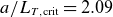 $a/L_{T,\text{crit}}=2.09$
. Left: boundary surface with magnetic field strength in colour. Centre: magnetic field line contours and field strength at
$a/L_{T,\text{crit}}=2.09$
. Left: boundary surface with magnetic field strength in colour. Centre: magnetic field line contours and field strength at
 $r=0.5a$
. Right: cross-section with several surfaces plotted at zero toroidal VMEC angle, at or near the maximum field strength. Note the higher compression of the surfaces on the outboard where the curvature drive is minimal.
$r=0.5a$
. Right: cross-section with several surfaces plotted at zero toroidal VMEC angle, at or near the maximum field strength. Note the higher compression of the surfaces on the outboard where the curvature drive is minimal.

Nonlinear heat flux calculations with adiabatic electrons for the three configurations discussed in the paper, scanning in temperature gradient
 $a/L_{T}$
at
$a/L_{T}$
at
 $r/a=0.5$
. Two flux tubes (at
$r/a=0.5$
. Two flux tubes (at
 $\alpha =0$
and
$\alpha =0$
and
 $\alpha = \pi /n_{fp}$
) were simulated and the more unstable of the two is plotted, depending on the case. For QICG and IM,
$\alpha = \pi /n_{fp}$
) were simulated and the more unstable of the two is plotted, depending on the case. For QICG and IM,
 $\alpha =\pi /n_{fp}$
is more unstable, while for W7-X,
$\alpha =\pi /n_{fp}$
is more unstable, while for W7-X,
 $\alpha =0$
is more unstable. A naive extrapolation from the two points at
$\alpha =0$
is more unstable. A naive extrapolation from the two points at
 $a/L_{T}=(2.5,3.0)$
down to
$a/L_{T}=(2.5,3.0)$
down to
 $Q=0$
yields CGs which are in the neighbourhood of the model predictions from (2.7). Notice that the IM configuration has a more pronounced ‘foot’ (Zocco et al. Reference Zocco, Xanthopoulos, Doerk, Connor and Helander2018) below the calculated CG, suggesting that more extended ITG modes survive in this geometry.
$Q=0$
yields CGs which are in the neighbourhood of the model predictions from (2.7). Notice that the IM configuration has a more pronounced ‘foot’ (Zocco et al. Reference Zocco, Xanthopoulos, Doerk, Connor and Helander2018) below the calculated CG, suggesting that more extended ITG modes survive in this geometry.

Profiles for the three configurations discussed in the paper at
 $2\,\%$
 $\beta$
. (a) Rotational transform as a function of the radial coordinate
$\beta$
. (a) Rotational transform as a function of the radial coordinate
 $s = (r/a)^2$
. (b) Magnetic well (
$s = (r/a)^2$
. (b) Magnetic well (
 $V$
is the volume enclosed by a flux surface) as a function of
$V$
is the volume enclosed by a flux surface) as a function of
 $s$
. (c) Neoclassical transport coefficient
$s$
. (c) Neoclassical transport coefficient
 $\epsilon _{\text{eff}}$
(Nemov et al. Reference Nemov, Kasilov, Kernbichler and Heyn1999) as a function of
$\epsilon _{\text{eff}}$
(Nemov et al. Reference Nemov, Kasilov, Kernbichler and Heyn1999) as a function of
 $s$
. (d) Geodesic curvature
$s$
. (d) Geodesic curvature
 $\kappa _{\text{geo}}a=a(\boldsymbol{B} \times \boldsymbol{\nabla } B) \boldsymbol{\cdot }\boldsymbol{\nabla } \psi / (B^{2} |\boldsymbol{\nabla } \psi |)$
at the surface
$\kappa _{\text{geo}}a=a(\boldsymbol{B} \times \boldsymbol{\nabla } B) \boldsymbol{\cdot }\boldsymbol{\nabla } \psi / (B^{2} |\boldsymbol{\nabla } \psi |)$
at the surface
 $s=0.25$
and field line
$s=0.25$
and field line
 $\alpha _{0}=0$
.
$\alpha _{0}=0$
.

4.1. The QI configurations
The starting point for the two new optimised QI configurations was a five-field-period configuration with zero axis helicity. We try to optimise for a high CG using the aforementioned targets, ignoring for the moment growth rates above the threshold. We find that it is necessary to optimise by checking
 $32$
flux tubes spanning 2 toroidal field periods to catch the most unstable spot on the flux surface. The optimisation is carried out targeting volume-averaged
$32$
flux tubes spanning 2 toroidal field periods to catch the most unstable spot on the flux surface. The optimisation is carried out targeting volume-averaged
 $\beta$
to be
$\beta$
to be
 $2\,\%$
using artificial, linear pressure profiles that peak at
$2\,\%$
using artificial, linear pressure profiles that peak at
 $r=0$
and are zero at
$r=0$
and are zero at
 $r=a$
. The edge toroidal flux is allowed to vary as an optimisation parameter to keep
$r=a$
. The edge toroidal flux is allowed to vary as an optimisation parameter to keep
 $\beta$
at this value. We note here that both new configurations possess a low value of
$\beta$
at this value. We note here that both new configurations possess a low value of
 $\epsilon _{\text{eff}}$
as well as small geodesic curvature in comparison with the HM configuration (figure 6).
$\epsilon _{\text{eff}}$
as well as small geodesic curvature in comparison with the HM configuration (figure 6).
Geometric quantities entering the gyrokinetic equation for the three configurations, for a flux tube centred at the outboard midplane, including drift curvature, normalised magnetic field strength and
 $\boldsymbol{\nabla } \alpha$
. Top left: for W7-X HM, the metrics somewhat resemble those of a quasisymmetric stellarator near the outboard midplane (no curvature gap at
$\boldsymbol{\nabla } \alpha$
. Top left: for W7-X HM, the metrics somewhat resemble those of a quasisymmetric stellarator near the outboard midplane (no curvature gap at
 $\ell =0$
). Top right: the same but for the QICG configuration with
$\ell =0$
). Top right: the same but for the QICG configuration with
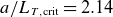 $a/L_{T,\text{crit}}=2.14$
, for which the ‘mode splitting’ is clearly visible in the curvature quantity
$a/L_{T,\text{crit}}=2.14$
, for which the ‘mode splitting’ is clearly visible in the curvature quantity
 $K_{d}$
, which shows two very separate bad curvature wells near the outboard midplane (near
$K_{d}$
, which shows two very separate bad curvature wells near the outboard midplane (near
 $\ell \sim \pm 4 a$
). Bottom centre: the IM configuration, similar to the previous case but with less pronounced splitting. The bad curvature has noticeably shifted away from the minimum of
$\ell \sim \pm 4 a$
). Bottom centre: the IM configuration, similar to the previous case but with less pronounced splitting. The bad curvature has noticeably shifted away from the minimum of
 $B$
.
$B$
.

The first new configuration, which we refer to as QI and Critical Gradient (QICG), was optimised for QI quality (see previous section), a vacuum magnetic well, an
 $\iota$
ranging from
$\iota$
ranging from
 $1.35$
to
$1.35$
to
 $1.50$
and an aspect ratio of
$1.50$
and an aspect ratio of
 $14$
. The targets used were
$14$
. The targets used were
 \begin{align} f_{QICG} & = f_{well} + f_{iota} + f_{CG} + f_{asp} \nonumber \\ & \quad + f_{mono} + f_{extrema} + f_{mirror} + f_{\beta } + f_{\overline {\epsilon }_{\text{eff}}}, \end{align}
with
 \begin{align} f_{asp}(A_{t}) = (A - 14)^{2}, \end{align}
(
 $A$
is the aspect ratio)
$A$
is the aspect ratio)
 \begin{align} f_{\iota }=\left [(\iota (s_{0}=0.0) - 1.35)^{2} + (\iota (s_{0}=1.0) - 1.49)^{2} \right ], \end{align}
and
 \begin{align} f_{well}=\sum _{r}\left [(1+V^{\prime \prime }(r)/0.01)\varTheta (1+V^{\prime \prime }(r)/0.01) \right ]^{2}, \end{align}
as in Roberg-Clark et al. (Reference Roberg-Clark, Plunk, Xanthopoulos, Nührenberg, Henneberg and Smith2023) with
 $r/a=\{0.0,0.25,0.95\}$
, and
$r/a=\{0.0,0.25,0.95\}$
, and
 \begin{equation} f_{\beta }=(\beta - 0.02)^{2}, \end{equation}
with
 $\beta$
the volume-averaged value calculated from VMEC. The targeted surfaces
$\beta$
the volume-averaged value calculated from VMEC. The targeted surfaces
 $r/a$
for
$r/a$
for
 $\epsilon _{\text{eff}}$
were
$\epsilon _{\text{eff}}$
were
 $r/a=(0.02,0.10,0.20,0.30,0.40,0.50,0.60,0.70,0.80,0.90)$
and varying weights were used for all of the terms over the course of the optimisation to prioritise at first QI quality and then the CG metric (2.8). The vacuum magnetic well (after removing pressure from the equilibrium) is roughly 0.25% (not shown), while at
$r/a=(0.02,0.10,0.20,0.30,0.40,0.50,0.60,0.70,0.80,0.90)$
and varying weights were used for all of the terms over the course of the optimisation to prioritise at first QI quality and then the CG metric (2.8). The vacuum magnetic well (after removing pressure from the equilibrium) is roughly 0.25% (not shown), while at
 $2\,\%$
 $\beta$
it has a low
$\beta$
it has a low
 $\epsilon _{\text{eff}}$
of roughly
$\epsilon _{\text{eff}}$
of roughly
 $0.2\,\%$
on axis. Figure 5 suggests that transport is relatively low below
$0.2\,\%$
on axis. Figure 5 suggests that transport is relatively low below
 $a/L_{T}=2.14$
and stays moderate above that point. The primary effect leading to the large CG of QICG is the mode splitting effect, which is clearly demonstrated in the top right-hand plot of figure 7, with an additional boost to
$a/L_{T}=2.14$
and stays moderate above that point. The primary effect leading to the large CG of QICG is the mode splitting effect, which is clearly demonstrated in the top right-hand plot of figure 7, with an additional boost to
 $g^{\alpha \alpha }$
through a localised shear effect.
$g^{\alpha \alpha }$
through a localised shear effect.
Nonlinear flux tube ITG simulations with kinetic electrons, a fixed temperature gradient
 $a/L_{T}=a/L_{T,i}=a/L_{T,e}=3$
and variable density gradient
$a/L_{T}=a/L_{T,i}=a/L_{T,e}=3$
and variable density gradient
 $a/L_{n}$
for both species at half-radius at the most unstable location. For W7-X, the flux tube is
$a/L_{n}$
for both species at half-radius at the most unstable location. For W7-X, the flux tube is
 $\alpha =0$
and for IM, it is
$\alpha =0$
and for IM, it is
 $\alpha =\pi /n_{fp}$
(see caption for figure 5). The heat flux for the IM case remains below or comparable to that of the W7-X HM configuration up to
$\alpha =\pi /n_{fp}$
(see caption for figure 5). The heat flux for the IM case remains below or comparable to that of the W7-X HM configuration up to
 $a/L_{n}=2$
.
$a/L_{n}=2$
.

Since we have not taken into account stability above the threshold, initial nonlinear results (not shown) reveal prohibitively large heat fluxes, likely exacerbated by the mode inertia effect. We re-optimise the QICG configuration so that the ITG growth rates are not too large, yielding the configuration we call ‘IM’. To reduce linear ITG growth rates with kinetic electrons, we construct a simple target that combines the factors discussed in §§ 2.5 and 2.6, which reads
 \begin{equation} f_{Q} = (\left [ \langle |\boldsymbol{\nabla } \alpha | \rangle (1 - \langle \epsilon (\ell ) \rangle _d ) \right ]^{-1} - t_{Q})^{2}, \end{equation}
with the averages calculated as in expression (2.9). Using a new set of targets
 \begin{equation} f_{IM} = f_{QICG} + f_{Q}, \end{equation}
with
 $t_{Q}=2.0$
(QICG values exceeded 3) as well as a CG of 2.0 (2.7), we arrive at the configuration in figure 4, with a significant positive (tokamak-like) shear, a rotational transform ranging from 1.3 to 0.98 (near targeted values
$t_{Q}=2.0$
(QICG values exceeded 3) as well as a CG of 2.0 (2.7), we arrive at the configuration in figure 4, with a significant positive (tokamak-like) shear, a rotational transform ranging from 1.3 to 0.98 (near targeted values
 $1.25$
to
$1.25$
to
 $1.01$
), an
$1.01$
), an
 $\epsilon _{\text{eff}}$
of roughly
$\epsilon _{\text{eff}}$
of roughly
 $0.2\,\%$
on axis (figure 6
c),
$0.2\,\%$
on axis (figure 6
c),
 $A=13$
(as targeted) and a vacuum magnetic well of
$A=13$
(as targeted) and a vacuum magnetic well of
 $0.17\,\%$
. In particular, the positive shear seems to be helpful for the mode inertia effect, as the bad curvature region appears to be shifted away from the minimum of
$0.17\,\%$
. In particular, the positive shear seems to be helpful for the mode inertia effect, as the bad curvature region appears to be shifted away from the minimum of
 $B$
. We see that the configuration has favourable heat fluxes compared with W7-X HM when kinetic electrons are included (figure 8).
$B$
. We see that the configuration has favourable heat fluxes compared with W7-X HM when kinetic electrons are included (figure 8).
5. Conclusion
This paper has presented a series of physics-motivated model targets for turbulence optimisation in stellarators as well as a general strategy for increasing CGs that we refer to as mode splitting. That the targets guide the optimisation towards ITG stability is shown with a series of example physics configurations that also possess or nearly possess a vacuum magnetic well. The first configuration shown has an approximate CG of
 $a/L_{T}=2.14$
, an unusually high value. The second configuration, which resembles an IM, maintains a similar CG while sacrificing some nonlinear stability for the case of adiabatic electrons, yet performs well in the presence of kinetic electrons via the so-called mode inertia effect (Costello & Plunk, Reference Costello and Plunk2025a
). Another property that distinguishes these configurations from previous QI results is that the minimum of the magnetic field strength is approximately poloidally straight in the Boozer plane. We argue that this is helpful in that deeply trapped particles will experience low values of geodesic curvature in their orbits. It remains to be seen how well
$a/L_{T}=2.14$
, an unusually high value. The second configuration, which resembles an IM, maintains a similar CG while sacrificing some nonlinear stability for the case of adiabatic electrons, yet performs well in the presence of kinetic electrons via the so-called mode inertia effect (Costello & Plunk, Reference Costello and Plunk2025a
). Another property that distinguishes these configurations from previous QI results is that the minimum of the magnetic field strength is approximately poloidally straight in the Boozer plane. We argue that this is helpful in that deeply trapped particles will experience low values of geodesic curvature in their orbits. It remains to be seen how well
 $\alpha$
-particle confinement can be improved in such configurations, which will require more careful attention towards improving QI quality, beyond simply targeting
$\alpha$
-particle confinement can be improved in such configurations, which will require more careful attention towards improving QI quality, beyond simply targeting
 $\epsilon _{\text{eff}}$
. We note here that analytic progress using optimal mode analysis (Plunk & Helander Reference Plunk and Helander2023; Costello & Plunk Reference Costello and Plunk2025b
) and model geometries (Rodriguez & Zocco Reference Rodriguez and Zocco2025) may also be helpful in refining CG estimates in the future.
$\epsilon _{\text{eff}}$
. We note here that analytic progress using optimal mode analysis (Plunk & Helander Reference Plunk and Helander2023; Costello & Plunk Reference Costello and Plunk2025b
) and model geometries (Rodriguez & Zocco Reference Rodriguez and Zocco2025) may also be helpful in refining CG estimates in the future.
Acknowledgments
We would like to thank A. Goodman for helpful tips on optimising QI configurations, in vacuum and at finite
 $\beta$
, and calculating vacuum magnetic wells in simsopt, as well as sharing VMEC equilibrium plotting routines. We thank P. Helander, P. Costello, M. Landreman, W. Sengupta, E. Paul, E. Rodríguez and R. Nies for helpful advice and discussions.
$\beta$
, and calculating vacuum magnetic wells in simsopt, as well as sharing VMEC equilibrium plotting routines. We thank P. Helander, P. Costello, M. Landreman, W. Sengupta, E. Paul, E. Rodríguez and R. Nies for helpful advice and discussions.
Editor Peter Catto thanks the referees for their advice in evaluating this article.
Funding
This work has been carried out within the framework of the EUROfusion Consortium, funded by the European Union via the Euratom Research and Training Programme (Grant Agreement No 101052200 – EUROfusion). Views and opinions expressed are, however, those of the author(s) only and do not necessarily reflect those of the European Union or the European Commission. Neither the European Union nor the European Commission can be held responsible for them.
Declaration of interest
The authors report no conflict of interest.


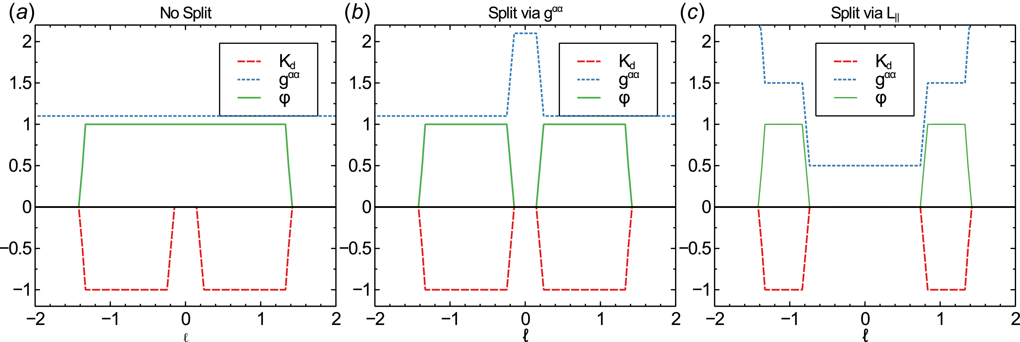


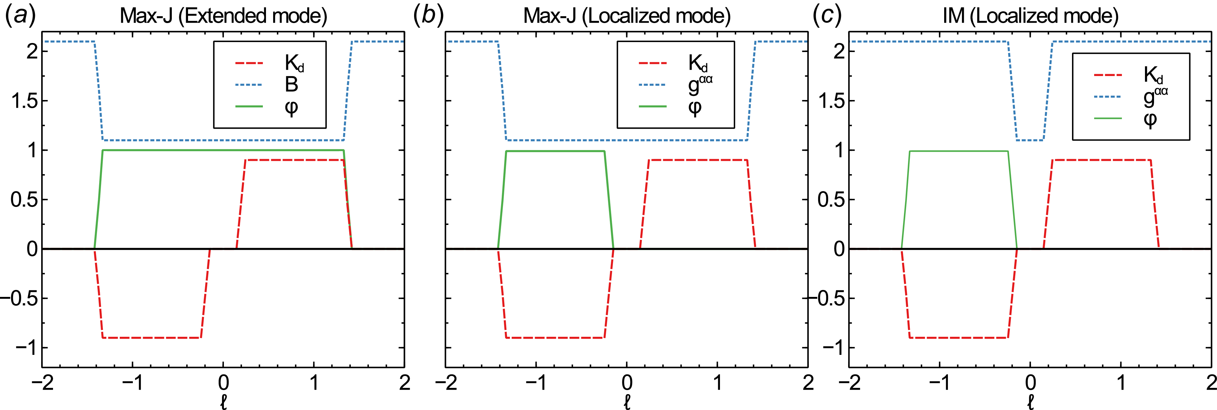


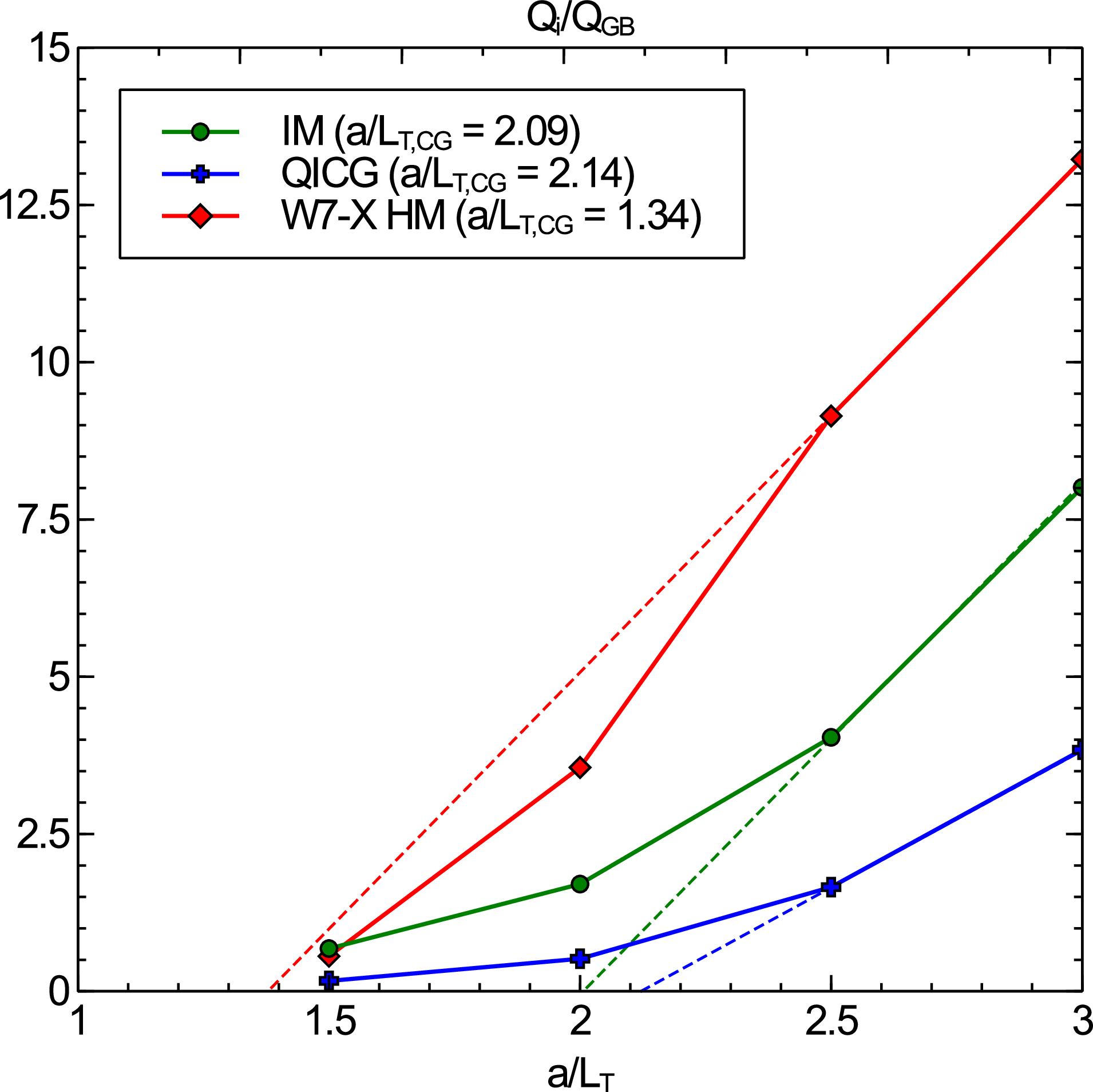


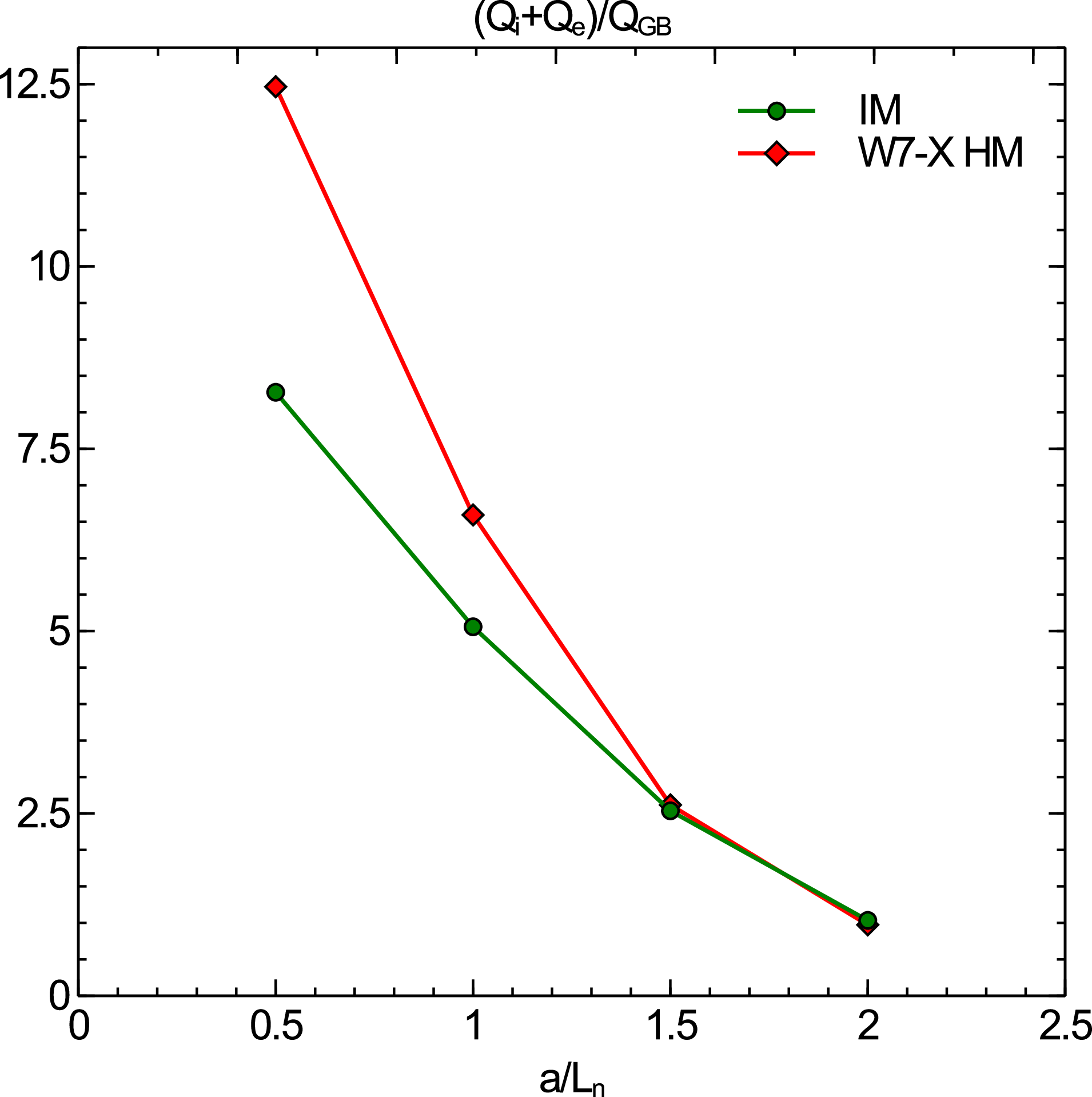


 Open access