


1. Introduction
The age of big data has witnessed a rapid generation and accumulation of flow data, both numerically and experimentally (Duraisamy, Iaccarino & Xiao Reference Duraisamy, Iaccarino and Xiao2019). Even standing on top of data, on most occasions, it remains not a simple task to understand a fluid flow due to the broad range that the flow may involve in its temporal and spatial scales. On the other hand, a complete dataset may not always be available. The extraction of pertinent knowledge from projected flow data (e.g. from flow visualisations) represents immense potentials for practical applications (Raissi, Yazdani & Karniadakis Reference Raissi, Yazdani and Karniadakis2020).
The development of model reduction and modal analysis techniques has played an essential role in promoting this effort (see reviews by Rowley & Dawson (Reference Rowley and Dawson2017) and Taira et al. (Reference Taira, Brunton, Dawson, Rowley, Colonius, McKeon, Schmidt, Gordeyev, Theofilis and Ukeiley2017, Reference Taira, Hemati, Brunton, Sun, Duraisamy, Bagheri, Dawson and Yeh2020)). With these approaches, a flow field has been decomposed into modes ranked by their inherent properties, e.g. energy, frequency or growth rate. For example, proper orthogonal decomposition (POD) (Lumley Reference Lumley, Yaglom and Tatarski1967) determines the optimal set of modes that represent most of the energy based on the  $L_2$ norm. The optimality lies both in the least possible number of modes to represent the signal and in the minimisation of error between the signal and its truncated representation. Dynamic mode decomposition (DMD) (Schmid Reference Schmid2010), on the other hand, arranges modes in the order of their dynamical importance that is measured by a characteristic frequency and growth rate. In essence, DMD is a finite-dimensional approximation to the Koopman operator (Rowley et al. Reference Rowley, Mezić, Bagheri, Schlatter and Henningson2009). For nonlinear problems, choosing a suitable set of observables as input is critical to maintain the link to the Koopman operator. Various improvements to the standard POD and DMD have been proposed. For example, balanced POD (Rowley Reference Rowley2005) weighs controllability and observability of a state by forming a biorthogonal set, and therefore is more suitable for non-normal systems. Spectral POD (Towne, Schmidt & Colonius Reference Towne, Schmidt and Colonius2018) reconsiders POD in the frequency domain, providing orthogonal modes (still ranked by energy) at discrete frequencies. Sparsity promoting DMD (Jovanović, Schmid & Nichols Reference Jovanović, Schmid and Nichols2014) reduces the dimensionality of the full rank decomposition, and recursive DMD (Noack et al. Reference Noack, Stankiewicz, Morzyński and Schmid2016) achieves orthogonality, an essential property of POD. Both POD and DMD are purely data-driven, in contrast to model-based linear global stability analysis (Theofilis Reference Theofilis2011) and resolvent analysis (McKeon & Sharma Reference McKeon and Sharma2010), which require an accurate base flow as well as the construction of a linearised operator. From the point of view of the stochastic process, Towne et al. (Reference Towne, Schmidt and Colonius2018) showed the inherent connection between DMD, resolvent analysis and spectral POD, indicating their common ground in mathematics.
The above-reviewed data-based decompositions aim at extracting dominant structures from a series of snapshots, while in the present work, an image-based technique will be introduced to obtain meaningful structures from instantaneous flow data, even though it can also apply to a sequence of snapshots. This technique is cost-effective and supports real-time analysis of flows upon observations.
Image-based flow decomposition hinges on the basis of the empirical wavelet transform (EWT) (Gilles Reference Gilles2013, Reference Gilles2020). Wavelet transform was recognised as a powerful technique in fluid mechanics not long after its advent (see early review by Farge Reference Farge1992). The pioneering work of Meneveau (Reference Meneveau1991) brings turbulence to the orthonormal wavelet space. Knowledge of turbulent kinetic energy, energy transfer and nonlinear interactions was obtained by physically interpreting the wavelet coefficients. In the examination of fluid flow data, wavelet analysis has been widely used as a flexible ‘microscope’ discriminating scales and positions simultaneously. The coherent vortex extraction (CVE) proposed by Farge, Pellegrino & Schneider (Reference Farge, Pellegrino and Schneider2001) splits turbulent flows into coherent and incoherent parts. Such CVE achieves its goal by projecting the vorticity field onto an orthogonal wavelet basis, and a threshold on the resulting wavelet coefficients is then specified to identify the coherent component. In the last decade, wavelet-based numerical algorithms and turbulence modelling have been developed (Schneider & Vasilyev Reference Schneider and Vasilyev2010). Their strengths lie in the ability to unambiguously identify and isolate localised, dynamically dominant flow structures which improves the efficiency of the computation. The EWT provides the first mathematically rigorous method to adaptively analyse a signal (Gilles Reference Gilles2013). The principal idea is to build a set of adaptive filter banks based on the property of the input signal itself, such that meaningful modes are extracted, each possessing a particular section of the Fourier supports. This feature matches well with the requirement to extract modes from instantaneous flow data or their visualisation.
In § 2, the formulation and algorithm of EWT for flow decompositions are introduced. In § 3 are provided two examples of EWT being applied to three-dimensional (3-D) instantaneous flow data and/or their visualisation, followed by a comparison with other methods in § 4. The study is concluded in § 5.
2. Imaged-based flow decomposition using EWT
We term the complete flow dataset or the visualisation (image or video) as a function  $f(x,y,z;t)$. Here $x$,
$x$,  $y$ and $z$ represent the spatial coordinates, and the optional $t$ denotes time. Note that flow visualisations project data onto a two-dimensional (2-D) image or video: $f(x,y;t)$. The visualisation may be qualitative and aided by auxiliary materials (e.g. smoke, sensitive coatings), or be quantitatively made with state-of-the art facilities (e.g. particle image velocimetry) or from numerical simulations (e.g. using
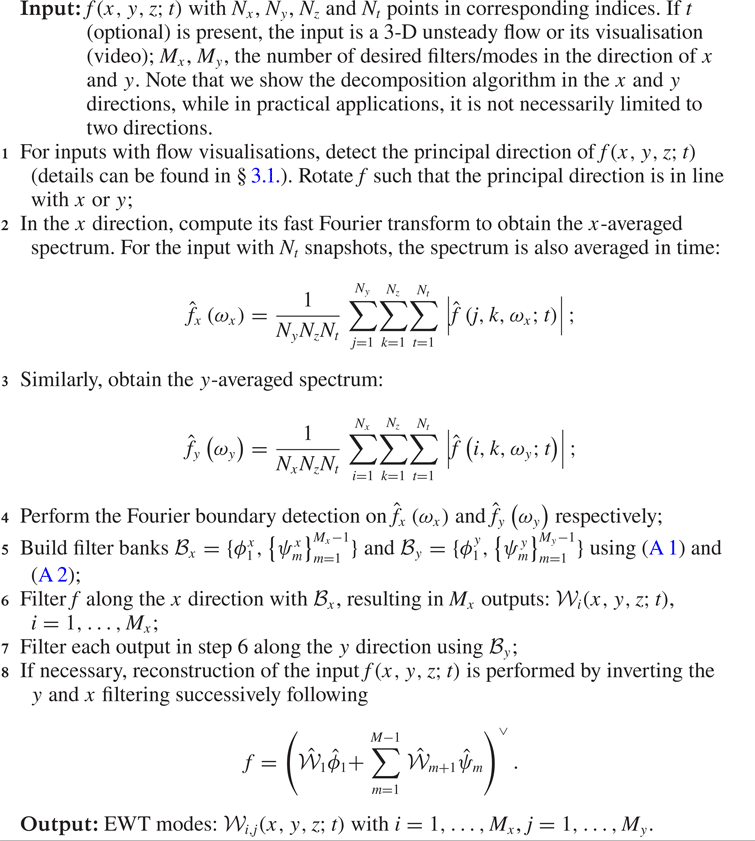
  $\lambda _2$ criterion (Jeong & Hussain Reference Jeong and Hussain1995) to identify vortex structures). We decompose the flow using 2-D tensor EWT (Gilles, Tran & Osher Reference Gilles, Tran and Osher2014) as summarised in algorithm 1. We aim to keep a limited number of resulting EWT modes which are sufficient to reveal the complex flow structures.
The EWT defines its scaling function  $\hat {\phi }_{m}$ and empirical wavelets $\hat {\psi }_{m}$ (see appendix A) in a normalised Fourier axis with $2{\rm \pi}$ periodicity. The set $\{ \phi _{1},\{ \psi _{m}\} _{m=1}^{M-1}\}$ is a tight and orthogonal frame of $L^{2}(\mathbb {R})$. Consequently, the ‘energy’ of the signal is conserved by the extracted EWT modes. The EWT of a signal $f(t)$ is obtained by
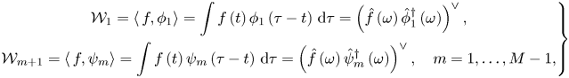 \begin{align} \left. \begin{gathered} \mathcal{W}_{1}=\left\langle\, f,\phi_{1}\right\rangle =\int f\left(t\right)\phi_{1}\left(\tau-t\right)\,\mathrm{d}\tau=\left(\hat{f}\left(\omega\right)\hat{\phi}_{1}^{\dagger}\left(\omega\right)\right)^{\vee},\\ \mathcal{W}_{m+1}=\left\langle\, f,\psi_{m}\right\rangle =\int f\left(t\right)\psi_{m}\left(\tau-t\right)\,\mathrm{d}\tau=\left(\hat{f}\left(\omega\right)\hat{\psi}_{m}^{\dagger}\left(\omega\right)\right)^{\vee},\quad m=1,\ldots,M-1, \end{gathered} \right\} \end{align}
where  $\langle \ \rangle$ stands for the inner product, $\dagger$ is the complex conjugate and $\wedge$ and $\vee$ indicate the Fourier transform and its inverse.
Flow decomposition using 2-D tensor EWT.
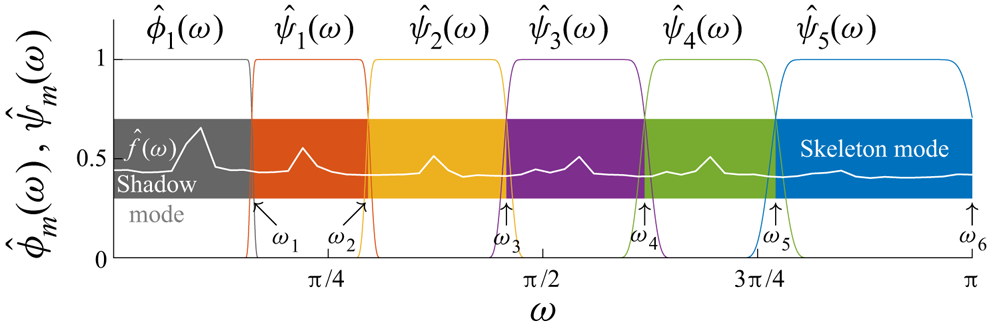
We show in figure 1 an example of the adaptive filter bank. The signal in Fourier space  $\hat {f}(\omega )$ is shown with a white line. A discussion of various Fourier supports $\{\omega _m\}$ detection strategies can be found in Gilles et al. (Reference Gilles, Tran and Osher2014). In this study, they are adaptively determined such that local maxima of $\hat {f}(\omega )$ are retained in different Fourier segments (indicated with different colours). As a result, the extracted modes strategically capture components of the input signal, each standing for a section of the spectrum. The idea of 2-D tensor EWT is to perform EWT successively in two directions, with the corresponding filter banks built according to the spatial-averaged spectrum. When flow visualisation is used as an input, it is essential to have the principal direction of the flow (e.g. direction of the mean flow) coincide with either direction of decomposition, such that the averaged spectrum maximises its physical relevance. This corresponds to step 1 of algorithm 1 and is detailed with an example in § 3.1.
A sketch in the Fourier space of the signal  $\hat {f}(\omega )$, the detected supports $\{\omega _m\}$ ( $m=1, 2,\ldots ,M$) and the filter bank $\{\hat {\phi }_1(\omega ), \hat {\psi }_1(\omega ), \hat {\psi }_2(\omega ),\ldots , \hat {\psi }_{M-1}(\omega )\}$. Here $\omega \in [0,{\rm \pi} ]$ and abides by the Nyquist–Shannon sampling theorem. The Fourier supports are determined from the spectrum of the signal $\hat {f}(\omega )$ such that each EWT mode amounts to part of the spectrum. The first and the last EWT modes, $\mathcal {W}_1$ and $\mathcal {W}_{M}$, are termed the shadow mode and the skeleton mode, respectively.
3. Applications and results
We show two applications of flow decomposition using EWT: the interaction between a 2-D wake and a jet plume, and an early-stage boundary layer transition subject to free-stream turbulence. The two examples serve to demonstrate the applicability to both flow data and their visualisation, irrespective of their experimental or numerical origin.
3.1. Interaction between a jet plume and a 2-D wake (images from experiments)
In this example, the decomposition is applied to the experimental observation of the interaction between a jet plume and a 2-D wake (Roquemore et al. Reference Roquemore, Britton, Tankin, Boedicker, Whitaker and Trump1988). The slot jet is located in the centre of the rectangular face of a bluff body. The flow is visualised with the reactive Mie scattering technique, where streamlines are highlighted by TiO $_2$ particles that are spontaneously formed by the reaction of TiCl $_4$ in the jet with water in the wake. The flow visualisation is shown in the first column of figure 2 with jet velocity increasing from $18.5\ \textrm {cm}\ \textrm {s}^{-1}$ in figure 2(a) to $55.5\ \textrm {cm}\ \textrm {s}^{-1}$ in figure 2(c). As introduced in Roquemore et al. (Reference Roquemore, Britton, Tankin, Boedicker, Whitaker and Trump1988), the flow is initially dominated by the wake flow when the shear-layer velocity of the jet $U_{jet}$ is smaller. Along with the increase of $U_{jet}$ in figure 2(b), wake instabilities are considerably prohibited, and only wavy structures are observed. In figure 2(c), the flow is dominated by the jet instability as indicated by the change in the direction of rotation of the vortices.
Image-based flow decomposition of the interaction between a jet plume and a 2-D wake:  $(a)$
$(a)$  $U_{jet}=18.5\ \textrm {cm}\ \textrm {s}^{-1}$; $(b)$
$(b)$  $U_{jet}=37.0\ \textrm {cm}\ \textrm {s}^{-1}$ with the source image rotated $2^{\circ }$ counterclockwise; $(c)$
$(c)$  $U_{jet}=55.5\ \textrm {cm}\ \textrm {s}^{-1}$. The wake is subject to an annular air flow at a constant velocity of $27.5\ \textrm {cm}\ \textrm {s}^{-1}$.
The flow decomposition is performed with  $M_x=M_y=3$, leading to nine EWT modes, ${\mathcal {W}_{i,j}}$ ( $i,j=1,2,3$). The lower modes (columns 2–5 of figure 2) well isolate key components of the flows. In particular, mode $\mathcal {W}_{1,1}$ (the shadow mode), comprising the lower-end spectrum in both the flow and transverse directions, can be used to detect the principal direction of the flow. Mode $\mathcal {W}_{2,1}$ possesses mid-spectrum in the transverse direction and features the mean flow. Representing the mid-spectrum of the flow direction, modes $\mathcal {W}_{1,2}$ and $\mathcal {W}_{2,2}$ present the flow instabilities with $\mathcal {W}_{2,2}$ accounting for higher wavenumbers in the transverse direction. Comparing the three cases adheres to the intention of the experiment: an increase of the jet velocity leads to the suppression of wake instabilities (figure 2b) and promotion of the jet instability downstream (figure 2c), as is supported by $\mathcal {W}_{2,2}$ in figure 2(a–c). It is also helpful to inspect the flow by combining certain modes: $\mathcal {W}_{1,1}\oplus \mathcal {W}_{2,1}$ and $\mathcal {W}_{1,2}\oplus \mathcal {W}_{2,2}$. The combination is obtained by performing an inverse EWT with corresponding modes. As is shown, $\mathcal {W}_{1,1}\oplus \mathcal {W}_{2,1}$ and $\mathcal {W}_{1,2}\oplus \mathcal {W}_{2,2}$ account for a wider spectrum in the transverse direction and differentiate in the flow direction, thus delivering a more comprehensive view of the mean flow and wake/jet instabilities, respectively. We have reconstructed the higher modes (the last column of figure 2) with $\mathcal {W}_{1,3}\oplus \mathcal {W}_{3,1}\oplus \mathcal {W}_{2,3}\oplus \mathcal {W}_{3,2}\oplus \mathcal {W}_{3,3}$. The higher modes account for the rest of the spectrum and retain all the small scales of the visualisation. Note that by increasing the number of EWT modes, the higher modes (the skeleton) will contain less information of the input.
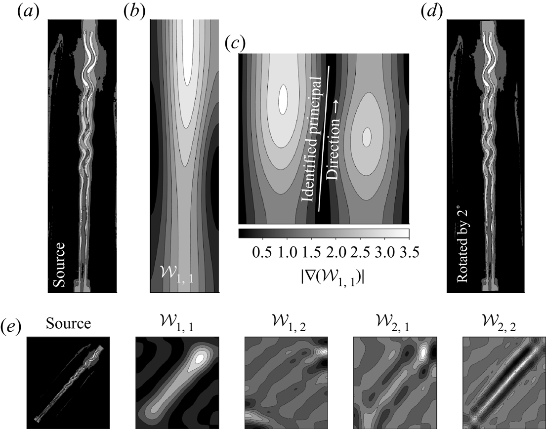
Recalling algorithm 1, in 2-D tensor EWT, the wavelet filter bank is built based on the averaged spectrum in the  $x$ and $y$ directions of the signal. It is crucial that the principal direction of the flow (e.g. the direction of the mean flow, orientations of the geometry) coincides with these directions, such that the flow physics can be correctly separated. In the $37.0\ \textrm {cm}\ \textrm {s}^{-1}$ case of the visualisation under consideration, we have rotated the source counterclockwise by $2.0^{\circ }$ before the EWT is applied (step 1 of algorithm 1). We take this case as an example to show how to accurately detect the principal direction. As shown in figure 3, the shadow mode $\mathcal {W}_{1,1}$, which is free from small scales, characterises the principal direction of the signal. This direction is thus numerically recovered by the gradient, $|\boldsymbol {\nabla }(\mathcal {W}_{1,1}) |$. The principal direction is the direction along which the average gradient reaches a minimum, as shown in figure 3(c). Consequently, it is found that the source shall be rotated counterclockwise by 2.0 $^{\circ }$. Figure 3(d) shows the rotated image as compared with figure 3(a). Figure 3(e) shows the decomposition when the source image has an inappropriate orientation at which $\mathcal {W}_{2,1}$ and $\mathcal {W}_{2,2}$ fail to capture the mean flow and instabilities.
Identification of the principal direction.  $(a)$ The source taken from the $U_{jet}=37.0\ \textrm {cm}\ \textrm {s}^{-1}$ case of Roquemore et al. (Reference Roquemore, Britton, Tankin, Boedicker, Whitaker and Trump1988). $(b)$
$(b)$  $\mathcal {W}_{1,1}$ of the original image. $(c)$ Image gradient of $\mathcal {W}_{1,1}$. For better display of the identified principal direction, the $x$–
$x$– $y$ aspect ratio is not to scale. $(d)$ The rotated image for flow decomposition. $(e)$ Flow decomposition based on the source with an inappropriate orientation.
3.2. Early-stage boundary layer transition (from direct numerical simulations)
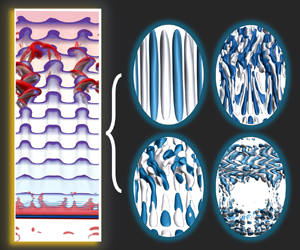
Laminar–turbulent transition prompts a significant broadening of flow scales that ultimately takes the form of coherent structures. This example examines an incompressible boundary layer flow over a flat plate with an elliptic leading edge (see figure 4). To promote flow transition, free-stream turbulence from a nonlinear optimisation procedure (with the target that the maximum perturbation energy is reached at a designated time) is specified ahead of the leading edge. The width of the domain is chosen such that three discernible streamwise-elongated streaks are generated. A periodic boundary condition is employed in the spanwise direction. Further numerical details and set-up of the simulations can also be found in Wang, Mao & Zaki (Reference Wang, Mao and Zaki2019). In this example, we first apply the algorithm to flow visualisation, followed by the decomposition with instantaneous 3-D velocity data.
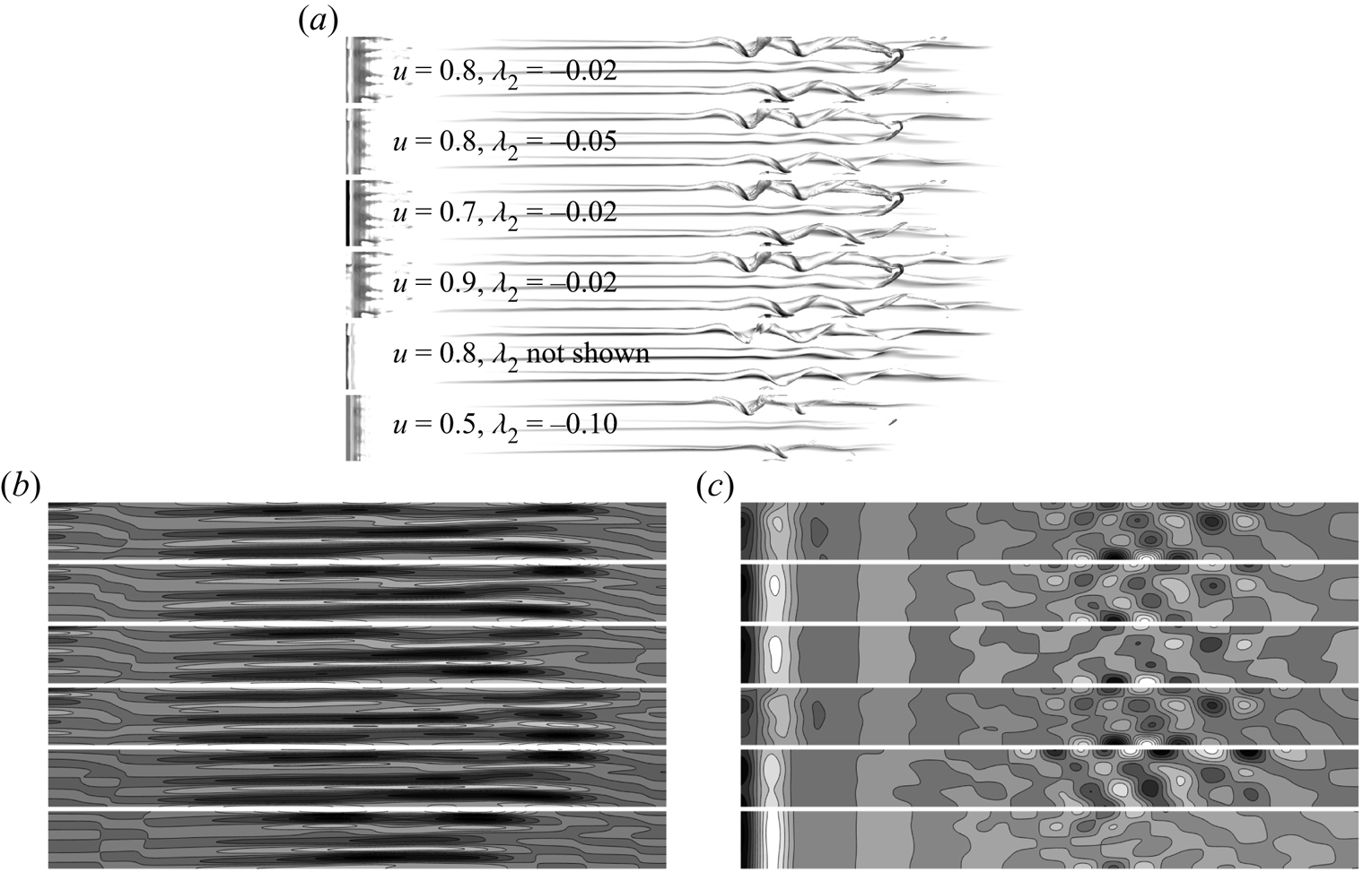
A schematic diagram of imaged-based flow decomposition with the example of boundary layer transition. The instantaneous flow field (3-D data) is visualised by iso-surfaces of  $\lambda _2=-0.02$ and $u=0.8$ together with contours of $u=0.1,0.2,\ldots ,0.9$ in cross-sections that are perpendicular to the free-stream direction. Both the iso-surfaces and contours are coloured by $u$. We apply imaged-based flow decomposition on the grey-scale 2-D image that contains the same iso-surfaces. The image has a top view on which the flow data in the wall-normal direction are projected. Within the computation domain, three discernible streaks are generated, and they become unstable downstream before giving rise to hairpin vortices.
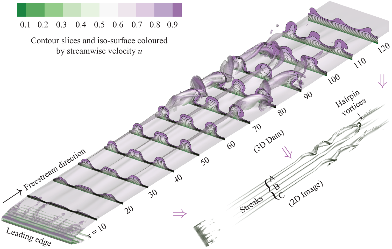
The flow has been visualised through its pivotal structures, i.e. with iso-surfaces of  $\lambda _2=-0.02$, $u=0.8$ and contour slices of $u=0.1, 0.2 ,\ldots , 0.9$ as presented in figure 4, where $u$ stands for the streamwise velocity (normalised by the free-stream value). A grey-scale top-view image with the same iso-surfaces serves as the input of the image-based flow decomposition. As can be seen, the 2-D image features the generation of streaks and the formation of hairpin vortices.
We show the flow decomposition in figure 5(a). In this example, we have  $M_x=M_z=3$. By construction, modes ${\mathcal {W}_{1,1}}$ (shadow mode) and ${\mathcal {W}_{3,3}}$ (skeleton mode) represent the flow structure with a spectrum that amounts to the lower and higher end in both the streamwise and spanwise directions. Modes ${\mathcal {W}_{1,2}}$ and ${\mathcal {W}_{1,3}}$ isolate the streaks. The secondary instabilities of streaks are captured by modes ${\mathcal {W}_{2,1}}$, ${\mathcal {W}_{2,2}}$ and ${\mathcal {W}_{2,3}}$, featuring the low to high wavenumbers in the spanwise direction. From ${\mathcal {W}_{2,1}}$, it is seen that Streak A gives rise to sinuous instabilities after $x=40$, followed by the instability of Streak C. It also indicates that perturbations around Streak C have a larger amplitude after $x=70$. These observations are, however, hidden in the source image. Finally, in modes ${\mathcal {W}_{3,1}}$ and ${\mathcal {W}_{3,2}}$, localised helical vortex filaments are identified, marking the meandering of streaks and appearance of smaller scales. $(a)$ Image-based flow decomposition of boundary layer transition. Here $M_x=M_z=3$, leading to nine EWT modes. Important streamwise locations $x=44$ (onset of secondary instabilities), $x=50, 70$ (base flows and eigenfunctions as seen in panel c) and $x=99$ (formation of hairpin vortices) are highlighted. White dashed lines in $\mathcal {W}_{2,1}$, $\mathcal {W}_{2,2}$, $\mathcal {W}_{2,3}$ show the position of streaks and the streamwise range over which secondary instabilities occur. $(b)$ Growth rates of the secondary instabilities versus streamwise wavenumber $\alpha$ at cross-sections of $x=43,44,45,50,70$. The red cross marker indicates the maximum growth rate of a mode whose eigenfunction is visualised in (c). The eigenfunction $u^{\prime }$ is shown with black lines (dashed lines denote negative values) on top of the base flow contours ( $u=0.1, 0.2,\ldots ,0.9$). A movie of the video-based flow decomposition is available as a supplementary movie available at https://doi.org/10.1017/jfm.2020.817.
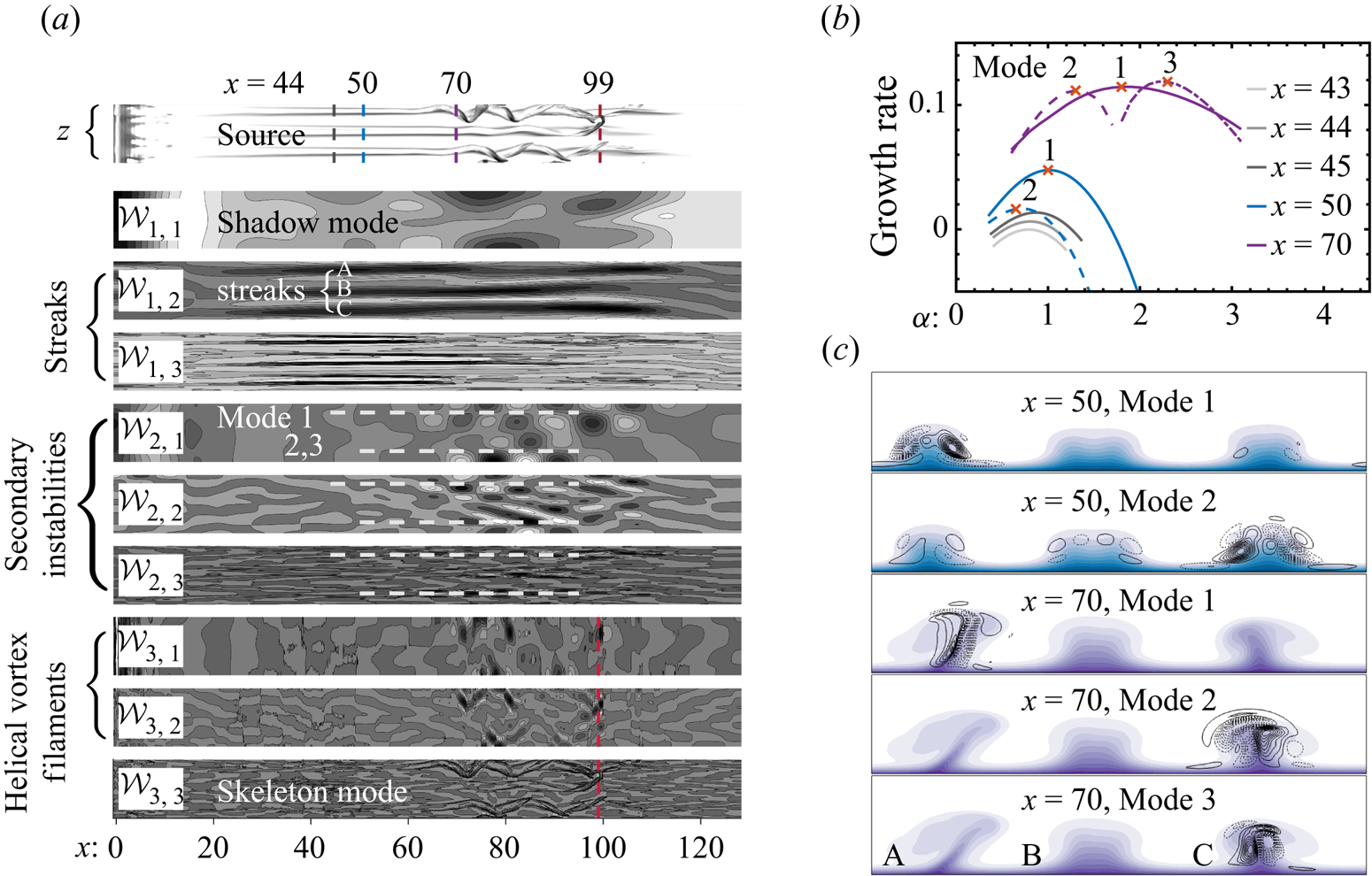
To verify the observation from EWT modes, a 2-D stability analysis (secondary instability of streaks) is performed at  $x=43,44,45$ (to secure the onset location of secondary instabilities) and $x=50,70$ (to identify multiple modes). We plot temporal growth rates versus streamwise wavenumber $\alpha$ in figure 5(b). The peak growth rates are marked with red crosses, and the corresponding eigenfunctions and base flows are provided in figure 5(c). A positive growth rate is seen at $x=44$, which demonstrates the onset of secondary instabilities. This mode (termed mode 1) has its eigenfunctions localised around Streak A. Further downstream, the flow is unstable to multiple modes. From around $x=50$, mode 2 (centred around Streak C) also becomes unstable, though at a smaller growth rate. However, further downstream at $x=70$, mode 3 (centred around Streak C) becomes the most energetic. All these secondary instability modes are of sinuous nature. Generally, the stability analysis matches rather well with EWT modes; the onset of multiple secondary instability modes, their sinuous nature and the dominance of instabilities around Streak C are evidenced by mode ${\mathcal {W}_{2,1}}$. For the case of a video input, an unsteady flow decomposition is provided as a supplementary movie. The video records the flow from $t=0$ when free-stream turbulence is introduced to the laminar flow until the time step illustrated in figures 4 and 5. The video-based EWT modes provide the evolution of flow structures subject to the temporal–spatial averaged Fourier supports.
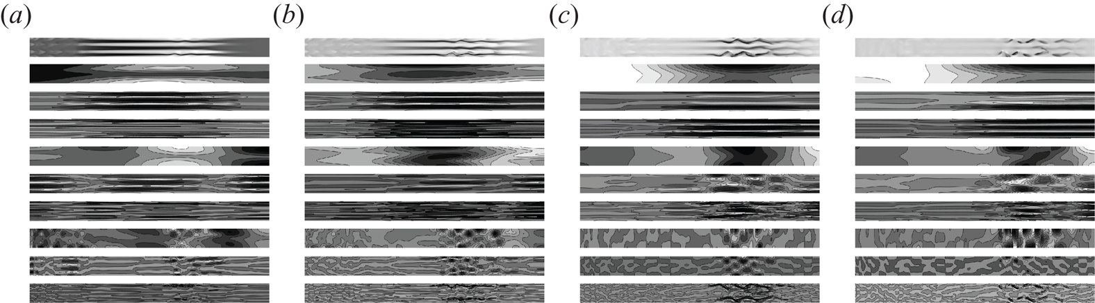
To test the sensitivity and robustness of the method with respect to the input image, a comparison of EWT modes with different flow visualisations is shown in figure 6. Images with various iso-surfaces of  $u$ and $\lambda _{2}$ are adopted as shown in figure 6(a). The same filter banks from EWT are used to process these inputs. As can be seen from figures 6(b) and 6(c), the streaks and their secondary instabilities are correctly extracted by modes $\mathcal {W}_{1,2}$ and $\mathcal {W}_{2,1}$ for most of the cases, regardless of the different inputs. With iso-surfaces of $u$ alone, secondary instabilities are captured, but the importance of Streak C is not revealed. For a more inimical input ( $u=0.5, \lambda _{2}=-0.10$), the EWT modes still result in satisfactory decompositions. Besides, it has been tested that the decomposition is robust to changes in lighting and shading of the visualisation. $(a)$ Flow visualisations of boundary layer transition with iso-surfaces of $u$ and $\lambda _{2}$ at values indicated on the image. (b,c) The corresponding EWT modes: $\mathcal {W}_{1,2}$ and $\mathcal {W}_{2,1}$.
In addition to these robustness tests, considering different choices of flow data, e.g. Reynolds decomposed velocity perturbations (Jacobs & Durbin Reference Jacobs and Durbin2001), we present decomposition for such inputs in figure 7. The input data are obtained at four horizontal sections, i.e.  $y=0.50\delta$, $y=0.75\delta$, $y=1.00\delta$ and $y=1.25\delta$, where $\delta$ is the boundary layer thickness near the centre of the streamwise domain ( $x=60$). Unlike the source images used in figure 4, the inputs are essentially 2-D and represent flows at a certain height. For example, at $y=0.50\delta$, streaks are mostly visible plus some wavy structures downstream, while $y=0.75\delta$ and $y=1.00\delta$ show the secondary instabilities primarily. Outside of the boundary layer at $y=1.25\delta$, the helical vortex filaments become dominant. These variations are appropriately captured by their EWT modes.
The EWT as applied to Reynolds decomposed streamwise velocity perturbations at horizontal sections:  $(a)$
$(a)$  $y=0.50\delta$, $(b)$
$(b)$  $y=0.75\delta$, $(c)$
$(c)$  $y=1.00\delta$, $(d)$
$(d)$  $y=1.25\delta$. Here $\delta$ is the boundary layer thickness near the centre of the streamwise domain ( $x=60$). In each panel, the first image shows the input data while the EWT modes follow and are arranged in the same order as in figure 5(a).
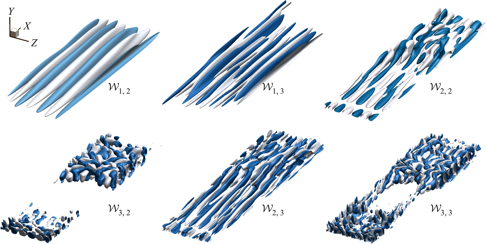
We further apply EWT to the decomposition of 3-D instantaneous data, as shown in figure 8. The flow has been decomposed in the  $x$ and $z$ directions with $M_x=M_z=3$ based on the streamwise velocity $u(x,y,z)$ on each $y$ plane. We show the physically significant modes with iso-surfaces. As can be seen, the streamwise-elongated streaks and their nonlinear harmonics are extracted by $\mathcal {W}_{1,2}$ and $\mathcal {W}_{1,3}$. Modes $\mathcal {W}_{2,2}$ and $\mathcal {W}_{3,2}$ capture streak instabilities at different scales. Modes $\mathcal {W}_{2,3}$ and $\mathcal {W}_{3,3}$ represent the higher-end spectrum in the spanwise direction, displaying the canonical bypass nature of the transition process, i.e. small scales in the free stream only reappear further downstream in the boundary layer leading to a ‘clean area’. Comparing the results presented in figures 5 and 8, both inputs of the instantaneous 3-D data and their visualisation lead to adaptively and physically relevant decompositions. The extracted streaks and their secondary instabilities from both results match well with each other and correctly reflect the flow physics. Note that when viewed and processed as an image, flow visualisation represents a projection of the 3-D instantaneous data, with the objective of compressing while retaining critical features of the data. Differences, as a result, stem from the discrepancy in the Fourier supports. For example, secondary instabilities are extracted by $\mathcal {W}_{2,1}$, $\mathcal {W}_{2,2}$ and $\mathcal {W}_{2,3}$ from the visualisation, while $\mathcal {W}_{2,2}$ and $\mathcal {W}_{3,2}$ from 3-D instantaneous data stand for streak instabilities. Another advantage of using flow data is that the extracted modes will have a solid physical meaning. For example, in this case, the modes are the decomposed streamwise velocities. Three-dimensional data further lead to more details of the flow, as evidenced by the bypass characteristics in $\mathcal {W}_{2,3}$ and $\mathcal {W}_{3,3}$.
Flow decomposition with 3-D velocity data  $u(x,y,z)$. The EWT is applied in the $x$ and $z$ directions with $M_x=M_z=3$. Iso-surfaces are defined and coloured (blue/white for positive/negative values) according to EWT modes: $\mathcal {W}_{1,2}$ ( $u={\pm }0.1$), $\mathcal {W}_{1,3}$ ( $u={\pm }0.05$), $\mathcal {W}_{2,2}$ ( $u={\pm }0.02$), $\mathcal {W}_{2,3}$ ( $u={\pm }0.01$), $\mathcal {W}_{3,2}$ ( $u={\pm }0.02$), $\mathcal {W}_{3,3}$ ( $u={\pm }0.01$).
4. Comparison with other methods
At this point, it becomes relevant to ask: what is the added value of EWT modes to the state-of-the-art data-based flow decompositions (e.g. the POD and DMD families)? This section takes the boundary layer transitional flow as an example to show the strengths and weaknesses of the proposed methods.
The flow case corresponds to the example shown in § 3.2. Time series as inputs for POD and DMD start from the initialisation of free-stream turbulence, encompassing the development of streamwise-elongated streaks and their secondary instabilities, and end at the snapshot shown in figure 4 where hairpin vortices appear. Figure 9 shows the decomposed flows using POD, DMD and EWT. These modes are illustrated with iso-surfaces of the streamwise velocity. From figure 9(d) it is evident that the first four POD modes cover most of the energy as displayed in figure 9(a). As can be seen, the most energetic structure is streamwise-elongated streaks. Modes 2 and 3 display a mixed structure of streaks and their instabilities. Mode 4, on the other hand, extracts smaller scales associated with the hairpin vortices. The DMD modes appear in pairs and are sorted by their frequencies. As expected, lower frequencies (modes 1 and 2 and modes 3 and 4) stand for streaks while the instabilities are captured in higher modes. The growth rates and amplitudes of DMD modes shown in figure 9(e,f) provide a soft criterion as a measure of the significance of the modes.
A comparison of POD, DMD and EWT modes. The POD  $(a)$ and DMD $(b)$ modes are extracted based on the velocity data $u(x,y,z,t)$ with the time series starting from the initiation of free-stream turbulence and ending at the snapshot shown in figure 4. The EWT modes $(c)$ are solely extracted from the instantaneous $u(x,y,z)$ corresponding to figure 4. The iso-surfaces are coloured with wall-normal coordinate and defined by $u=-4\times 10^{-4}$ of the extracted POD/DMD modes. The same iso-surface levels as in figure 8 are used for EWT modes. $(d)$ The energy distribution among POD modes. (e,f) The growth rate and amplitude of the DMD modes. The blue dots mark four (pairs of) dominating POD/DMD modes shown in (a,b).
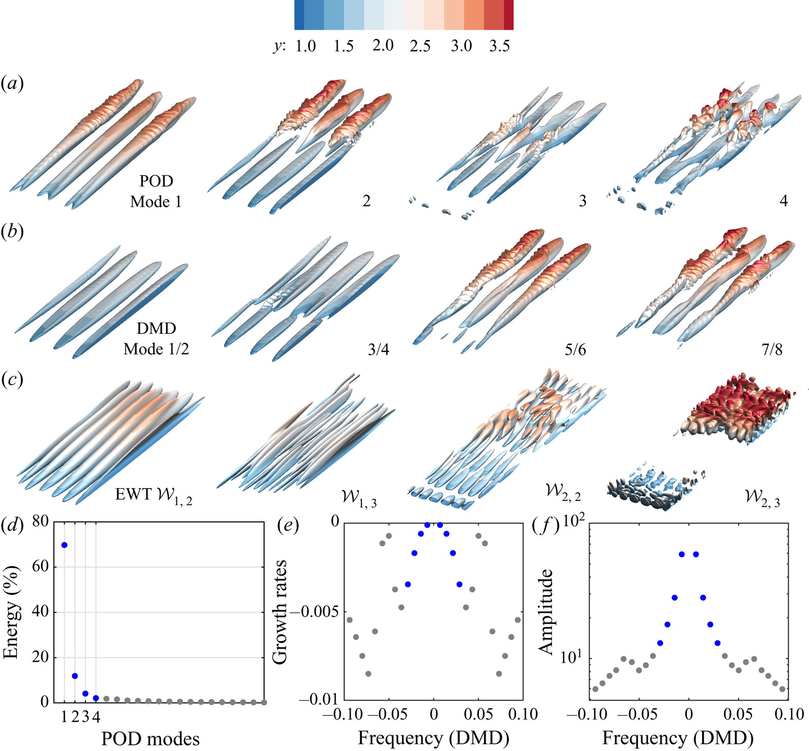
The EWT modes are obtained solely from a single snapshot corresponding to figure 4. Without resorting to time series, the flows are decomposed according to spatial scales. As a result, the streaks, their secondary instabilities and the bypass nature of smaller scales are distinctly identified.
On the aspect of outputs, all three methods can lead to an arbitrary number of modes. A notable question arises as to what is the effectiveness of the modes in characterising the flow. For example, how many modes would be sufficient to represent the flow and what are the criteria for selecting dominant modes? This has been recognised as a weakness of modal-based flow analysis (Taira et al. Reference Taira, Brunton, Dawson, Rowley, Colonius, McKeon, Schmidt, Gordeyev, Theofilis and Ukeiley2017). The POD modes are arranged according to their energy, which is a meaningful indication of importance. However, highly nonlinear or travelling wave problems may require a large number of POD modes to cover the majority of the energy (Murata, Fukami & Fukagata Reference Murata, Fukami and Fukagata2020). On the other hand, a single correct way to rank DMD modes is absent, though the growth rate and amplitude provide means of measurement. With regard to EWT, there is not a concomitant indicator (e.g. energy, frequency, growth rate) associated with the modes. Instead of producing a large number of modes and choosing a few important ones (e.g. in POD and DMD), EWT aims at generating a limited number of modes, differing only in spatial scales. We have shown that for flows with compact Fourier supports,  $M_{x}=M_{z}=3$ gives satisfactory results. However, for flows with a broader spatial spectrum, one may need to increase the number of modes to reduce the mixing of scales in extracted modes.
The EWT shares a similar theoretical basis, i.e. multi-resolution analysis, with CVE (Farge et al. Reference Farge, Pellegrino and Schneider2001). In CVE, wavelet coefficients are first obtained for the vorticity field using orthogonal wavelet transform. These coefficients are further divided into two groups (coherent and incoherent) according to their amplitudes. The coherent and incoherent flow components are therefore reconstructed through the inverse wavelet transform. By construction, the objective of CVE is to extract coherent structures based on the wavelet denoising method rather than decomposing a flow into several modes. Results of CVE for boundary layer transitional flow are provided in figure 10. For this case, the coherent structure is captured by only 0.8 % of the total wavelet coefficients, reflecting the sparse distribution in the wavelet space. Integrating the spirit of multi-resolution analysis into DMD creates multi-resolution DMD (Kutz, Fu & Brunton Reference Kutz, Fu and Brunton2016), which performs DMD recursively on a hierarchy of multi-resolution time scales. The method is a variation of the standard DMD. Still, it exhibits strengths in handling signals with multi-scale or invariant dynamics, while the present approach addresses multi-scale fluid structures in the spatial domain.
Coherent vortex extraction of the transitional boundary layer. The input is the streamwise vorticity  $\omega _{x}$. Iso-surfaces are defined and coloured by $\omega _{x}={\pm }0.1$ for the input and coherent component, while $\omega _{x}={\pm }0.06$ is used for the incoherent counterpart to increase visibility.

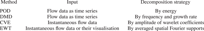
As such, it becomes clear that EWT provides a new decomposition strategy, as shown in table 1. Furthermore, EWT does not depend on a separation-of-variables strategy, which leads to its advantage in dealing with non-stationary flows or travelling wave problems.
A comparison of POD, DMD, CVE and EWT.
5. Concluding remarks
In this paper, we have proposed an image-based flow decomposition using the 2-D tensor EWT (Gilles Reference Gilles2013; Gilles et al. Reference Gilles, Tran and Osher2014), which was initially devised for image processing. According to the Fourier supports of the input data, a set of adaptive filter banks (an orthogonal frame) is built to perform the decomposition. A first example considers the interactions between a 2-D wake and a jet plume, where only experimental flow visualisations are available. The EWT modes correctly isolate the jet and wake components and their instabilities. In the spirit of 2-D tensor EWT, the visualisation principal direction needs to coincide with one of the decomposition directions. We show that this direction can be accurately determined using the shadow mode of EWT,  $\mathcal {W}_{1,1}$. The second example considers an early-stage boundary layer transition subject to free-stream turbulence, where direct numerical simulation provided a full dataset. For both inputs of 3-D instantaneous flow data and their visualisation, the EWT modes distinctly extract streamwise-elongated streaks, their secondary instabilities and smaller scales. A comparison with 2-D stability analysis justifies the EWT modes that characterise the secondary instabilities. The bypass nature of smaller scales is also captured by EWT modes based on the 3-D instantaneous flow data.
Compared with the prevailing data-based methods for flow decomposition (POD, DMD and CVE, to name a few), EWT offers a new strategy to adaptively decompose a flow from its averaged Fourier supports. An instantaneous flow or its visualisation is thus readily decomposed without resorting to its time series. The method also functions well on non-stationary flows or travelling wave problems by extracting fluid physics that are localised from the input. Still, it would be less effective for flows with broader or flattened Fourier supports, e.g. fully developed turbulent flows, where the number of EWT modes needs to be in line with the spatial spectrum of the flow. In future development, the method can be extended to account for the temporal spectrum and the prediction of flow evolution.
Acknowledgements
This investigation is funded by the European Union's Horizon 2020 future and emerging technologies programme with agreement no. 828799. Calculations were performed on HPC-Midlands funded by the Engineering and Physical Sciences Research Council (grant no. EP/K000063/1).
Declaration of interests
The authors report no conflict of interests.
Supplementary movie
Supplementary movie is available at https://doi.org/10.1017/jfm.2020.817.
Appendix A. Scaling function and empirical wavelets of EWT
The scaling function  $\hat {\phi }_{m}$ and empirical wavelets $\hat {\psi }_{m}$ of EWT (Gilles Reference Gilles2013) are given by
 \begin{gather} \hat{\phi}_{m}\left(\omega\right)=\begin{cases} 1 & \mathrm{if}\ \left|\omega\right|\leq\left(1-\gamma\right)\omega_{m},\\ \cos\left[\dfrac{\rm \pi}{2}\beta\left(\dfrac{\left|\omega\right|-\left(1-\gamma\right)\omega_{m}}{2\gamma\omega_{m}}\right)\right] & \mathrm{if}\ \left(1-\gamma\right)\omega_{m}\leq\left|\omega\right|\leq\left(1+\gamma\right)\omega_{m},\\ 0 & \mathrm{otherwise}, \end{cases} \end{gather}
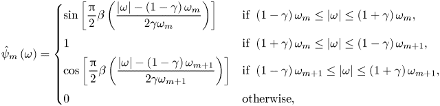 \begin{gather} \hat{\psi}_{m}\left(\omega\right)=\begin{cases} \sin\left[\dfrac{\rm \pi}{2}\beta\left(\dfrac{\left|\omega\right|-\left(1-\gamma\right)\omega_{m}}{2\gamma\omega_{m}}\right)\right] & \mathrm{if}\ \left(1-\gamma\right)\omega_{m}\leq\left|\omega\right|\leq\left(1+\gamma\right)\omega_{m},\\ 1 & \mathrm{if}\ \left(1+\gamma\right)\omega_{m}\leq\left|\omega\right|\leq\left(1-\gamma\right)\omega_{m+1},\\ \cos\left[\dfrac{\rm \pi}{2}\beta\left(\dfrac{\left|\omega\right|-\left(1-\gamma\right)\omega_{m+1}}{2\gamma\omega_{m+1}}\right)\right] & \mathrm{if}\ \left(1-\gamma\right)\omega_{m+1}\leq\left|\omega\right|\leq\left(1+\gamma\right)\omega_{m+1},\\ 0 & \mathrm{otherwise}, \end{cases} \end{gather}
 \begin{gather} \textrm{with}\ \beta\left(x\right)=\begin{cases} 0 & \mathrm{if}\ x\leq0,\\ x^{4}\left(35-84x+70x^{2}-20x^{3}\right) & \mathrm{if}\ 0 < x < 1,\\ 1 & \mathrm{if}\ x\geq1. \end{cases} \end{gather}
 \begin{gather} \mathrm{If}\ \gamma<\underset{m}{\min}\left(\frac{\omega_{m+1}-\omega_{m}}{\omega_{m+1}+\omega_{m}}\right),~\mathrm{then}~\stackrel[k=-\infty]{\infty}{\sum}\left(\left|\hat{\phi}_{1}\left(\omega+2k{\rm \pi}\right)\right|^{2}+\stackrel[m=1]{N}{\sum}\left|\hat{\psi}_{m}\left(\omega+2k{\rm \pi}\right)\right|^{2}\right)=1. \end{gather}
The set  $\{ \phi _{1},\{ \psi _{m}\} _{m=1}^{M-1}\}$ forms a tight and orthogonal frame of $L^{2}(\mathbb {R})$. Note that in the theory of wavelet frames, a frame is termed tight if the energy of the extracted wavelet coefficients is directly proportional to the original signal with a factor of $A$. Furthermore, if $A=1$, the frame is defined as orthogonal.


 Open access