





1 Introduction
A cline describes a gradual change in genotypic frequency as a function of spatial location. The existence of a cline often depends on gene selection and migration, as well as the scale of favourable habitat. Studying the generation patterns and stability of clines can provide scientific theoretical support for species protection measures and biomedical therapies.
The first mathematician to analyse migration and selection was Fisher [Reference Fisher9]. In 1948, Haldane [Reference Haldane11] derived a reaction-diffusion equation for the equilibrium allele frequencies at a diallelic locus subject to spatially varying selection along a single spatial dimension. This work is generally regarded as the earliest mathematical theory of clines. The study of clines became a very active research area beginning in the 1970s, when the consequences of various assumptions about spatial variation in fitness and about migration patterns were investigated (see, for example, [Reference Nagylaki18–Reference Nakashima26, Reference Nakashima, Ni and Su29, Reference Slatkin32]). Meanwhile, Conley [Reference Conley2], Fleming [Reference Fleming10], Fife and Peletier [Reference Fife and Peletier7, Reference Fife and Peletier8] and Henry [Reference Henry12] developed and employed advanced mathematical methods to investigate the existence, uniqueness and stability of clinal solutions under a variety of assumptions about fitness. Since the beginning of the new century, Lou et al. [Reference Hofbauer and Su13–Reference Lou, Ni and Su17, Reference Nakashima27, Reference Nakashima28] extended previous work in several directions by modelling migration with general elliptic operators on bounded domains in arbitrary dimensions. Recently, Su et al. [Reference Su, Lam and Bürger33] provided conditions for the existence and linear stability of a two-locus cline when recombination is either sufficiently weak or sufficiently strong relative to selection and diffusion. More recently, using the bifurcation analysis method, Nakashima and Tsujikawa [Reference Nakashima and Tsujikawa30] studied positive stationary solutions for a problem arising from population genetics.
Let A and a denote the alleles at the locus under consideration. In his celebrated work, Nagylaki [Reference Nagylaki18] derived the following semi-infinite Neumann problem [Reference Amster and Déboli1]:
 $$ \begin{align} \begin{cases} \dfrac{{d}^2 p}{{d}\xi^2}+k^2g(\xi)p(1-p)=0,& \xi>0,\\ \dfrac{{d} p}{{d}\xi}=0& \text{at}\ 0,+\infty, \end{cases} \end{align} $$
where p is the gene frequency of A, $k^2=(2sa^2)/\sigma ^2$
with
$k^2=(2sa^2)/\sigma ^2$
with $k>0$
is the combination of the selection intensity
$k>0$
is the combination of the selection intensity $s>0$
, advantageous habitat scale
$s>0$
, advantageous habitat scale $a>0$
, migration variance
$a>0$
, migration variance $\sigma ^2/2$
and
$\sigma ^2/2$
and $sg(\xi )$
with
$sg(\xi )$
with
 $$ \begin{align*} g(\xi)= \begin{cases} 1, &0\leq \xi\leq1,\\ -\alpha^2, &\xi>1, \end{cases} \end{align*} $$
the Malthusian parameter or the selection coefficient for the genotype $AA$
. Here,
$AA$
. Here, $-\alpha ^2$
, with
$-\alpha ^2$
, with $\alpha>0$
, is the ratio of the selection coefficients for
$\alpha>0$
, is the ratio of the selection coefficients for $\xi>1$
and
$\xi>1$
and $0 \leq \xi \leq 1$
. Let
$0 \leq \xi \leq 1$
. Let $p_0=p(0)$
. By studying the relationship between
$p_0=p(0)$
. By studying the relationship between $p_0$
and k, Nagylaki obtained that
$p_0$
and k, Nagylaki obtained that $k>\arctan \alpha $
is a necessary and sufficient condition for a unique solution of (1.1), which corresponds to a unique cline. Here,
$k>\arctan \alpha $
is a necessary and sufficient condition for a unique solution of (1.1), which corresponds to a unique cline. Here, $\arctan \alpha :=k_1$
denotes the first positive root of
$\arctan \alpha :=k_1$
denotes the first positive root of $\tan k=\alpha $
. In fact, he only obtained the unique
$\tan k=\alpha $
. In fact, he only obtained the unique $p_0$
. Obviously,
$p_0$
. Obviously, $p_0$
can be determined by p, but the converse is not true. Therefore, it is clearly necessary to study the existence and uniqueness of p. The derivation by Nagylaki [Reference Nagylaki18, (31)] assumed the boundary condition
$p_0$
can be determined by p, but the converse is not true. Therefore, it is clearly necessary to study the existence and uniqueness of p. The derivation by Nagylaki [Reference Nagylaki18, (31)] assumed the boundary condition $\lim _{\xi \rightarrow +\infty }p=0$
. Here, from now on, we also assume that the solution p in (1.1) satisfies
$\lim _{\xi \rightarrow +\infty }p=0$
. Here, from now on, we also assume that the solution p in (1.1) satisfies $\lim _{\xi \rightarrow +\infty }p=0$
. When the unfavourable habitat is infinite, it is reasonable for the cline to approach
$\lim _{\xi \rightarrow +\infty }p=0$
. When the unfavourable habitat is infinite, it is reasonable for the cline to approach $0$
. This also indicates that when the unfavourable habitat is infinite,
$0$
. This also indicates that when the unfavourable habitat is infinite, $1$
is not in equilibrium, which is consistent with biological reality. Therefore, this assumption is both realistic and reasonable.
$1$
is not in equilibrium, which is consistent with biological reality. Therefore, this assumption is both realistic and reasonable.
Furthermore, he also conjectured that the cline is stable. To the best of our knowledge, this conjecture has not yet been fully resolved. This is also the main motivation for this work. Moreover, does the cline p (rather than $p_0$
) form a solution curve with respect to k? What is the decay rate of a cline p at infinity? What is the stability of the trivial solution
$p_0$
) form a solution curve with respect to k? What is the decay rate of a cline p at infinity? What is the stability of the trivial solution $p=0$
? We will provide satisfactory answers to these questions here.
$p=0$
? We will provide satisfactory answers to these questions here.
Define
 $$ \begin{align*} X=\bigg\{p\in C[0,+\infty)\mid p'(0)=0, \lim_{\xi\rightarrow+\infty}\frac{p e^{{\alpha k_1}\xi/{\sqrt{3}}}}{\xi}=0\bigg\} \end{align*} $$
endowed with the norm $\Vert p\Vert =\sup _{\xi \in [0,+\infty )}\vert p(\xi )\vert $
, which is clearly a Banach space. Let
$\Vert p\Vert =\sup _{\xi \in [0,+\infty )}\vert p(\xi )\vert $
, which is clearly a Banach space. Let $X^+=\{p\in X\mid p \geq 0\}$
with the deduced norm of X, and
$X^+=\{p\in X\mid p \geq 0\}$
with the deduced norm of X, and $P^+$
be the set of functions in
$P^+$
be the set of functions in $X^+$
which are positive in
$X^+$
which are positive in $[0,+\infty )$
. Also, set
$[0,+\infty )$
. Also, set $K^{+}=(0,+\infty )\times P^{+}$
under the product topology.
$K^{+}=(0,+\infty )\times P^{+}$
under the product topology.
The first main result of this work is the following theorem.
Theorem 1.1. The pair $(\arctan \alpha , 0)$
is a bifurcation point of problem (1.1) and the associated bifurcation curve
$(\arctan \alpha , 0)$
is a bifurcation point of problem (1.1) and the associated bifurcation curve $\mathcal {C}\subseteq (K^+\cup \{(\arctan \alpha ,0)\})$
is unbounded, approaching
$\mathcal {C}\subseteq (K^+\cup \{(\arctan \alpha ,0)\})$
is unbounded, approaching $1$
as
$1$
as $k\rightarrow +\infty $
. Moreover, for
$k\rightarrow +\infty $
. Moreover, for $k\leq \arctan \alpha $
, problem (1.1) has only the trivial solution
$k\leq \arctan \alpha $
, problem (1.1) has only the trivial solution $p=0$
; while for
$p=0$
; while for $k>\arctan \alpha $
, there is a unique solution p with
$k>\arctan \alpha $
, there is a unique solution p with $0<p\leq 1$
. In addition, for each
$0<p\leq 1$
. In addition, for each $(k,p)\in \mathcal {C}$
, p exponentially decays to
$(k,p)\in \mathcal {C}$
, p exponentially decays to $0$
at infinity.
$0$
at infinity.
Our conclusions indicate that $k>\arctan \alpha $
is a necessary and sufficient condition for the existence and uniqueness of a solution p, rather than merely
$k>\arctan \alpha $
is a necessary and sufficient condition for the existence and uniqueness of a solution p, rather than merely $p_0$
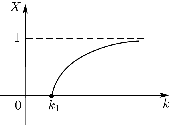
as in [Reference Nagylaki18]. Moreover, we also obtain a bifurcation curve (see Figure 1) and the decay rate of the cline p at
$p_0$
as in [Reference Nagylaki18]. Moreover, we also obtain a bifurcation curve (see Figure 1) and the decay rate of the cline p at $+\infty $
.
$+\infty $
.
Bifurcation diagrams of Theorem 1.1.

Figure 1 illustrates that a branch of positive solutions bifurcates from the trivial solution at the critical value $k_1 = \arctan \alpha $
. The solution branch exists exclusively for
$k_1 = \arctan \alpha $
. The solution branch exists exclusively for $k> k_1$
and converges to
$k> k_1$
and converges to $1$
as
$1$
as $k \to +\infty $
.
$k \to +\infty $
.
Regarding stability, we have the following result.
Theorem 1.2. For any $k>\arctan \alpha $
, the cline p is (asymptotically linearly) stable. For the trivial solution
$k>\arctan \alpha $
, the cline p is (asymptotically linearly) stable. For the trivial solution $p=0$
, it is (asymptotically linearly) stable for all
$p=0$
, it is (asymptotically linearly) stable for all $k<\arctan \alpha $
and unstable for each
$k<\arctan \alpha $
and unstable for each $k>\arctan \alpha $
.
$k>\arctan \alpha $
.
Our conclusion about the cline is consistent with Nagylaki’s expectation. It is also consistent with Slatkin’s numerical work [Reference Slatkin32]. Moreover, we also obtain the stability of the trivial solution $p=0$
. From a genetic perspective, stability indicates the dominance of selection. The expression for k shows that stronger selection and a larger favourable habitat both promote the survival of the cline. This is consistent with biological reality. The stability of the cline further suggests that such a genetic pattern, once established, can persist under small perturbations. These conclusions provide a theoretical basis for predicting species distribution limits and for designing conservation strategies in fragmented environments.
$p=0$
. From a genetic perspective, stability indicates the dominance of selection. The expression for k shows that stronger selection and a larger favourable habitat both promote the survival of the cline. This is consistent with biological reality. The stability of the cline further suggests that such a genetic pattern, once established, can persist under small perturbations. These conclusions provide a theoretical basis for predicting species distribution limits and for designing conservation strategies in fragmented environments.
The combination of an unbounded domain and a sign-changing weight function g poses substantial challenges for the analysis of this problem. Due to the unboundedness of the interval, it is often difficult to obtain the compactness of related operators using the compact embedding theorem (on bounded domain) or the Arzelà–Ascoli theorem. Of course, if the weight function has a good decay rate at infinity, it is also possible to get compactness. However, the weight function g here not only changes sign, but also lacks decay. We need to develop some new tricks to achieve our goals. Here, we find that the cline is exponentially decaying at infinity. Using this property, we can define a suitable work space X and obtain the compactness of the related operator. Thus, classical bifurcation theory can be used to study this problem.
Since the weight function g is sign-changing, it is difficult to directly use the conventional linearization method or stable exchange theory [Reference Crandall and Rabinowitz3, Reference Crandall and Rabinowitz4]. This may be the reason why Nagylaki’s stability conjecture has not been fully resolved so far. Noting $g\neq 0$
, we here overcome the difficulties caused by the sign change of g by simultaneously dividing the equation by g and then linearizing it. Furthermore, due to the sign change of the weight function g, the Rayleigh quotient for the first eigenvalue of the linearization problem may not necessarily exist, resulting in an indefinite sign of its corresponding eigenfunctions. We use the monotonicity of the cline and the piecewise constant nature of g to prove that the Rayleigh quotient for the first eigenvalue of the linearization problems does indeed exist. Furthermore, it is proven that the first eigenvalue of the linearization problem is the principal eigenvalue. Using this conclusion, the sign of the first eigenvalue of the linearization problem can be determined and the expected stability conclusion can be obtained from its sign.
$g\neq 0$
, we here overcome the difficulties caused by the sign change of g by simultaneously dividing the equation by g and then linearizing it. Furthermore, due to the sign change of the weight function g, the Rayleigh quotient for the first eigenvalue of the linearization problem may not necessarily exist, resulting in an indefinite sign of its corresponding eigenfunctions. We use the monotonicity of the cline and the piecewise constant nature of g to prove that the Rayleigh quotient for the first eigenvalue of the linearization problems does indeed exist. Furthermore, it is proven that the first eigenvalue of the linearization problem is the principal eigenvalue. Using this conclusion, the sign of the first eigenvalue of the linearization problem can be determined and the expected stability conclusion can be obtained from its sign.
Note that Nakashima et al. [Reference Nakashima25–Reference Nakashima28, Reference Nakashima and Tsujikawa30] studied indefinite diffusion problems on bounded domains with continuous and sign-changing weight functions. The present work considers a semi-infinite habitat with a piecewise-constant sign-changing weight, proving uniqueness and stability of the cline. Moreover, the nonlinear term they considered is bistable, that is, $u^ 2 (1-u)$
. While, we consider a logistic nonlinear term here, our conclusions complement those important results.
$u^ 2 (1-u)$
. While, we consider a logistic nonlinear term here, our conclusions complement those important results.
The rest of this paper is arranged as follows. In Section 2, we first study the spectrum of the linearization problem. Then, through an auxiliary problem, we prove that the cline satisfies $0<p\leq 1$
. Furthermore, we obtain the decay behaviour of p at infinity. Section 3 establishes the global bifurcation structure and proves the uniqueness of the solution, completing the proof of Theorem 1.1. In Section 4, we complete the proof of Theorem 1.2 by a complete stability analysis for both the trivial and nontrivial solutions. Finally, Section 5 concludes the paper.
$0<p\leq 1$
. Furthermore, we obtain the decay behaviour of p at infinity. Section 3 establishes the global bifurcation structure and proves the uniqueness of the solution, completing the proof of Theorem 1.1. In Section 4, we complete the proof of Theorem 1.2 by a complete stability analysis for both the trivial and nontrivial solutions. Finally, Section 5 concludes the paper.
2 Preliminary
We first study the spectrum of the linearization problem. It is not difficult to verify that the linearization problem of (1.1) at equilibrium point $0$
is
$0$
is
 $$ \begin{align} \begin{cases} \dfrac{{d}^2 p}{{d}\xi^2}+k^2g(\xi)p=0,& \xi>0,\\ \dfrac{{d} p}{{d}\xi}=0 &\text{at}\ 0,+\infty. \end{cases} \end{align} $$
By simple calculation, we can obtain
 $$ \begin{align*} p(\xi)= \begin{cases} A\cos(k\xi), &0\leq\xi\leq1,\\ Be^{-\alpha k \xi},&\xi>1. \end{cases} \end{align*} $$
Since p and $p'$
are continuous at
$p'$
are continuous at $\xi =1$
, we find that
$\xi =1$
, we find that $\alpha =\tan k$
. Thus, problem (2.1) only has a sequence of positive eigenvalues
$\alpha =\tan k$
. Thus, problem (2.1) only has a sequence of positive eigenvalues $k_i$
such that
$k_i$
such that
 $$ \begin{align*} (i-1)\pi<k_i<\frac{\pi}{2}+(i-1)\pi \quad \text{with}\ i\geq1. \end{align*} $$
Furthermore, the corresponding eigenfunction is generated by
 $$ \begin{align*} p_i(\xi)= \begin{cases} \cos(k_i\xi), &0\leq\xi\leq1,\\ \cos(k_i)e^{\alpha k_i(1- \xi)}, &\xi>1. \end{cases} \end{align*} $$
According to the range of $k_i$
, we see that
$k_i$
, we see that $\cos (k_i)\neq 0$
and, hence,
$\cos (k_i)\neq 0$
and, hence, $p_i(\xi )$
does not change sign for
$p_i(\xi )$
does not change sign for $\xi>1$
. Using the range of
$\xi>1$
. Using the range of $k_i$
again, we can see that
$k_i$
again, we can see that $\cos (k_i\xi )$
has exactly
$\cos (k_i\xi )$
has exactly $i-1$
simple zeros in
$i-1$
simple zeros in $(0,1)$
. In particular,
$(0,1)$
. In particular, $p_1$
is positive. For
$p_1$
is positive. For $i\geq 2$
, we can calculate the zeros of
$i\geq 2$
, we can calculate the zeros of $p_i$
as
$p_i$
as $\pi /(2k_i)$
,
$\pi /(2k_i)$
, $(3\pi )/(2k_i)$
,
$(3\pi )/(2k_i)$
, $\ldots $
,
$\ldots $
, $((2i-3)\pi )/(2k_i)$
.
$((2i-3)\pi )/(2k_i)$
.
In summary, we have the following conclusion regarding the spectrum of problem (2.1).
Proposition 2.1. Problem (2.1) only has a sequence of positive eigenvalues $k_i$
such that
$k_i$
such that
 $$ \begin{align*} (i-1)\pi<k_i<\frac{\pi}{2}+(i-1)\pi, \quad i\geq1. \end{align*} $$
The eigenfunction $p_i$
corresponding
$p_i$
corresponding $k_i$
has exactly
$k_i$
has exactly $i-1$
simple zeros
$i-1$
simple zeros $\pi /(2k_i)$
,
$\pi /(2k_i)$
, $(3\pi )/(2k_i)$
,
$(3\pi )/(2k_i)$
, $\ldots $
,
$\ldots $
, $((2i-3)\pi )/(2k_i)$
in
$((2i-3)\pi )/(2k_i)$
in $(0,1)$
. In particular,
$(0,1)$
. In particular, $p_1$
is positive.
$p_1$
is positive.
From Proposition 2.1, we can see $k_1<\pi /2$
and
$k_1<\pi /2$
and $k_2>\pi $
. It follows that
$k_2>\pi $
. It follows that $k_2-k_1>\pi /2$
, which holds in all parameter regimes. This explicit spectral gap estimate shows that
$k_2-k_1>\pi /2$
, which holds in all parameter regimes. This explicit spectral gap estimate shows that $k_1$
corresponds to the smallest admissible eigenvalue.
$k_1$
corresponds to the smallest admissible eigenvalue.
Since eigenfunction $p_i$
decays exponentially to
$p_i$
decays exponentially to $0$
at infinity, we have reason to believe that the nontrivial solution of problem (1.1) also decays exponentially to
$0$
at infinity, we have reason to believe that the nontrivial solution of problem (1.1) also decays exponentially to $0$
at infinity. To show this, we first study the range of solutions to problem (1.1). Define
$0$
at infinity. To show this, we first study the range of solutions to problem (1.1). Define
 $$ \begin{align*} f(s)= \begin{cases} 0 &\text{if}\ s<0,\\ s(1-s)&\text{if}\ 0\leq s\leq1,\\ 0&\text{if}\ s>1 \end{cases} \end{align*} $$
and consider the following auxiliary problem:
 $$ \begin{align} \begin{cases} \dfrac{{d}^2 p}{{d}\xi^2}+k^2g(\xi)f(p)=0,& \xi>0,\\ \dfrac{{d} p}{{d}\xi}=0 & \text{at} \ 0,+\infty. \end{cases} \end{align} $$
Then, we have the following lemma.
Lemma 2.2. For any nonconstant solution p of problem (2.2), one has that $0\leq p\leq 1$
and, hence, it is also the solution of problem (1.1).
$0\leq p\leq 1$
and, hence, it is also the solution of problem (1.1).
Proof. We only prove $p\leq 1$
, because the proof for
$p\leq 1$
, because the proof for $p\geq 0$
is similar. If p is always greater than
$p\geq 0$
is similar. If p is always greater than $1$
, one sees that
$1$
, one sees that $p"\equiv 0$
. Combining this with the boundary conditions implies that p is constant, which corresponds to a trivial solution. Therefore, there exists at least one point such that
$p"\equiv 0$
. Combining this with the boundary conditions implies that p is constant, which corresponds to a trivial solution. Therefore, there exists at least one point such that $p=1$
. From the definition of g and f, we can derive that p is decreasing. We use
$p=1$
. From the definition of g and f, we can derive that p is decreasing. We use $\xi _0$
to denote the first zero of
$\xi _0$
to denote the first zero of $p(\xi )=1$
. We suppose by contradiction that
$p(\xi )=1$
. We suppose by contradiction that $p(0)=\sup p>1$
. It follows that
$p(0)=\sup p>1$
. It follows that $p(\xi )>1$
for all
$p(\xi )>1$
for all $\xi <\xi _0$
. Using the definition of f again, we get
$\xi <\xi _0$
. Using the definition of f again, we get $p=a\xi +b$
in
$p=a\xi +b$
in $[0,\xi _0)$
. In view of the boundary condition
$[0,\xi _0)$
. In view of the boundary condition $p'(0)=0$
, we have
$p'(0)=0$
, we have $p=b$
in
$p=b$
in $[0,\xi _0)$
. Since
$[0,\xi _0)$
. Since $p(\xi _0)=1$
, we derive that
$p(\xi _0)=1$
, we derive that $b=1$
. Thus, we obtain
$b=1$
. Thus, we obtain $p\equiv 1$
in
$p\equiv 1$
in $[0,\xi _0]$
, which is a contradiction. This completes the proof.
$[0,\xi _0]$
, which is a contradiction. This completes the proof.
By Lemma 2.2, we only need to study the existence and uniqueness of nontrivial solutions for the auxiliary problem (2.2). We further claim that $0< p\leq 1$
for every nonconstant solution p of problem (2.2). To prove this, we first establish the following existence and uniqueness result.
$0< p\leq 1$
for every nonconstant solution p of problem (2.2). To prove this, we first establish the following existence and uniqueness result.
Lemma 2.3. If nonconstant function p satisfies problem (2.2) and it has a double zero, then $p \equiv 0$
.
$p \equiv 0$
.
Proof. Let p be such a function and $\xi _*$
be a double zero. It follows that
$\xi _*$
be a double zero. It follows that
 $$ \begin{align*} p=-k^2\int_{\xi_*}^\xi\int_{\xi_*}^s g(\tau)f(p)\,{d}\tau\,{d}s. \end{align*} $$
If $\xi \in [0, \xi _*]$
, in view of Lemma 2.2, we have
$\xi \in [0, \xi _*]$
, in view of Lemma 2.2, we have
 $$ \begin{align*} \vert p(\xi)\vert&\leq k^2 \int_{\xi_*}^\xi\int_{\xi_*}^s \vert g(\tau)f(p)\vert\,{d}\tau\,{d}s\\ &\leq k^2\max\, \{1,\alpha^2\} \int_{\xi_*}^\xi\int_{\xi_*}^s p\,{d}\tau\,{d}s\\ &\leq k^2\max\, \{1,\alpha^2\} \int_{\xi_*}^\xi\int_{\xi_*}^\xi p\,{d}\tau\,{d}s\\ &\leq k^2\max\, \{1,\alpha^2\} (\xi_*-\xi)\int_{\xi}^{\xi_*} p\,{d}\tau\\ &\leq k^2\max\, \{1,\alpha^2\}\xi_*\int_{\xi}^{\xi_*} p\,{d}s. \end{align*} $$
By the Gronwall–Bellman inequality [Reference Dai5, Lemma 2.2], we obtain that $p\equiv 0$
on
$p\equiv 0$
on $[0, \xi _*]$
.
$[0, \xi _*]$
.
However, when $\xi \in [\xi _*,b]$
for any fixed
$\xi \in [\xi _*,b]$
for any fixed $b>\xi _*$
, we have
$b>\xi _*$
, we have
 $$ \begin{align*} \vert p(\xi)\vert\leq k^2\max\, \{1,\alpha^2\}(b-\xi_*)\int_{\xi_*}^{\xi} p\,{d}s. \end{align*} $$
It follows from the modified version of the Gronwall–Bellman inequality [Reference Dai5, Lemma 2.1] that $p \equiv 0$
on
$p \equiv 0$
on $[\xi _*, b]$
. The arbitrariness of b implies
$[\xi _*, b]$
. The arbitrariness of b implies $p \equiv 0$
on
$p \equiv 0$
on $[\xi _*, +\infty )$
.
$[\xi _*, +\infty )$
.
If p is a nonconstant solution of problem (2.2), one has that $0\leq p\leq 1$
via Lemma 2.2. If p has a zero
$0\leq p\leq 1$
via Lemma 2.2. If p has a zero $\xi _1$
, since it is decreasing,
$\xi _1$
, since it is decreasing, $p(\xi )\equiv 0$
for
$p(\xi )\equiv 0$
for $\xi \geq \xi _1$
. By Lemma 2.3, we conclude that
$\xi \geq \xi _1$
. By Lemma 2.3, we conclude that $p(\xi )\equiv 0$
, which is impossible. In conclusion, we obtain the following lemma.
$p(\xi )\equiv 0$
, which is impossible. In conclusion, we obtain the following lemma.
Lemma 2.4. For any nonconstant solution p of problem (2.2), one has that $0< p\leq 1$
and, hence, it is also the solution of problem (1.1).
$0< p\leq 1$
and, hence, it is also the solution of problem (1.1).
From Lemma 2.4, we see that $p_0\in (0,1]$
. Further, if
$p_0\in (0,1]$
. Further, if $p_0$
is unique, Lemmas 2.2, 2.3 and 2.4 imply that the solution p with
$p_0$
is unique, Lemmas 2.2, 2.3 and 2.4 imply that the solution p with $p(0)=p_0$
of problem (1.1) is also unique. It should be pointed out that here, we use the auxiliary problem (2.2) to prove
$p(0)=p_0$
of problem (1.1) is also unique. It should be pointed out that here, we use the auxiliary problem (2.2) to prove $p_0\in (0,1]$
, rather than assuming it as in [Reference Nagylaki18].
$p_0\in (0,1]$
, rather than assuming it as in [Reference Nagylaki18].
Now, we return to the decay rate of a nonconstant solution p of problem (2.2) at $+\infty $
. We have known that
$+\infty $
. We have known that $0< p\leq 1$
. Further, we have the following result.
$0< p\leq 1$
. Further, we have the following result.
Proposition 2.5. Let p be a nonconstant solution of (2.2). Then, for $\xi>1$
, we have
$\xi>1$
, we have
 $$ \begin{align*} \widetilde{p}_1e^{-\alpha k(\xi-1)}<p\leq \widetilde{p}_1 e^{-{\alpha k(\xi-1)}/{\sqrt{3}}}, \end{align*} $$
where $\widetilde {p}_1=p(1)$
.
$\widetilde {p}_1=p(1)$
.
Proof. Since p satisfies $\lim _{\xi \rightarrow +\infty }p(\xi )=0$
, from [Reference Nagylaki18, (31)], we know that
$\lim _{\xi \rightarrow +\infty }p(\xi )=0$
, from [Reference Nagylaki18, (31)], we know that
 $$ \begin{align*} \alpha k(\xi-1)=\int_p^{\widetilde{p}_1}\frac{1}{s(1-{2s}/{3})^{1/2}}\,{d}s. \end{align*} $$
Since $0< p\leq 1$
, we find that
$0< p\leq 1$
, we find that
 $$ \begin{align*} \ln \frac{\widetilde{p}_1}{p}=\int_p^{\widetilde{p}_1}\frac{1}{s}\,{d}s<\alpha k(\xi-1)\leq \sqrt{3}\int_p^{\widetilde{p}_1}\frac{1}{s}\,{d}s=\sqrt{3} \ln \frac{\widetilde{p}_1}{p}, \end{align*} $$
which further implies the desired conclusion.
Proposition 2.5 indicates the nontrivial solution of problem (2.2) decays exponentially to $0$
at infinity if it satisfies
$0$
at infinity if it satisfies $\lim _{\xi \rightarrow +\infty }p(\xi )=0$
. Further, we have the following result.
$\lim _{\xi \rightarrow +\infty }p(\xi )=0$
. Further, we have the following result.
Lemma 2.6. If p is any nonconstant solution of problem (2.2) and satisfies $\lim _{\xi \rightarrow +\infty }p(\xi )=0$
, then for
$\lim _{\xi \rightarrow +\infty }p(\xi )=0$
, then for $\xi>1$
, we have
$\xi>1$
, we have
 $$ \begin{align*} \lim_{\xi\rightarrow+\infty}\frac{p e^{{\alpha k_1\xi}/{\sqrt{3}}}}{\xi}=0, \end{align*} $$
where $k_1$
is the first eigenvalue of problem (2.1).
$k_1$
is the first eigenvalue of problem (2.1).
Proof. From Proposition 2.5, we know that $0< p\leq 1$
and
$0< p\leq 1$
and
 $$ \begin{align*} p\leq \widetilde{p}_1 e^{-{\alpha k(\xi-1)}/{\sqrt{3}}}. \end{align*} $$
We claim that $k>k_1$
. If it was
$k>k_1$
. If it was $k\leq k_1$
, we have
$k\leq k_1$
, we have
 $$ \begin{align*} \frac{{d}^2 p}{{d}\xi^2}+k^2g(\xi)p(1-p)=0. \end{align*} $$
We also note that
 $$ \begin{align*} \frac{{d}^2 p_1}{{d}\xi^2}+k_1^2g(\xi)p_1=0. \end{align*} $$
Multiplying the equation for p by $p_1$
and integrating by parts gives
$p_1$
and integrating by parts gives
 $$ \begin{align} \int_0^{+\infty}p'p'_1\,{d}\xi=\int_0^{+\infty}k^2gpp_1(1-p)\,{d}\xi. \end{align} $$
We have known that p is decreasing. Proposition 2.5 implies that p is not a nonzero constant. Hence, $p' \leq 0$
and
$p' \leq 0$
and $p' \not \equiv 0$
. Since
$p' \not \equiv 0$
. Since $p_1$
is strictly decreasing, we conclude that
$p_1$
is strictly decreasing, we conclude that
 $$ \begin{align} \int_0^{+\infty}gpp_1(1-p)\,{d}\xi>0. \end{align} $$
Furthermore, multiplying the equation for $p_1$
by p and integrating by parts, then subtracting (2.3) and using (2.4), we find that
$p_1$
by p and integrating by parts, then subtracting (2.3) and using (2.4), we find that
 $$ \begin{align} 0&=k^2\int_0^{+\infty}gpp_1(1-p)\,{d}\xi-\int_0^{+\infty}k_1^2gpp_1\,{d}\xi \nonumber\\ &\leq k_1^2\int_0^{+\infty}gpp_1(1-p)\,{d}\xi-\int_0^{+\infty}k_1^2gpp_1\,{d}\xi\nonumber\\ &=-k_1^2\int_0^{+\infty}gp^2p_1\,{d}\xi. \end{align} $$
However, multiplying the equation for $p_1$
by
$p_1$
by $p^2$
and integrating by parts yields
$p^2$
and integrating by parts yields
 $$ \begin{align} 2\int_0^{+\infty}pp_1'p'\,{d}\xi=k_1^2\int_0^{+\infty}gp^2p_1\,{d}\xi. \end{align} $$
Because $p' \leq 0$
,
$p' \leq 0$
, $p' \not \equiv 0$
and
$p' \not \equiv 0$
and $p_1$
is strictly decreasing, we have
$p_1$
is strictly decreasing, we have
 $$ \begin{align*} \int_0^{+\infty}pp_1'p'\,{d}\xi>0. \end{align*} $$
Combining this with (2.6) shows that
 $$ \begin{align*} \int_0^{+\infty}gp^2p_1\,{d}\xi>0. \end{align*} $$
Now, in view of (2.5), we derive that
 $$ \begin{align*} 0\leq-k_1^2\int_0^{+\infty}gp^2p_1\,{d}\xi<0, \end{align*} $$
which is absurd.
Therefore, we have that
 $$ \begin{align*} p< \widetilde{p}_1 e^{-{\alpha k_1(\xi-1)}/{\sqrt{3}}}. \end{align*} $$
It follows that
 $$ \begin{align*} \frac{pe^{{\alpha k_1\xi}/{\sqrt{3}}}}{\xi}<\frac{\widetilde{p}_1}{\xi}e^{{\alpha k_1}/{\sqrt{3}}}\rightarrow0 \end{align*} $$
as $\xi \rightarrow +\infty $
, which implies the desired conclusion. This completes the proof.
$\xi \rightarrow +\infty $
, which implies the desired conclusion. This completes the proof.
Finally, we present a Rabinowitz-type global bifurcation result [Reference Dai5, Lemma 2.5]. Let E be a real Banach space with the norm $\Vert \cdot \Vert $
,
$\Vert \cdot \Vert $
, $\mathcal {O}$
be an open subset of
$\mathcal {O}$
be an open subset of $\mathbb {R}\times E$
,
$\mathbb {R}\times E$
, $\text {pr}_E(\mathcal {O})$
be the projection of
$\text {pr}_E(\mathcal {O})$
be the projection of $\mathcal {O}$
on E and
$\mathcal {O}$
on E and $\text {pr}_{\mathbb {R}}(\mathcal {O})$
be the projection of
$\text {pr}_{\mathbb {R}}(\mathcal {O})$
be the projection of $\mathcal {O}$
on
$\mathcal {O}$
on $\mathbb {R}$
. Consider the following operator equation:
$\mathbb {R}$
. Consider the following operator equation:
 $$ \begin{align} u= L(\lambda)u+H(\lambda,u):=G(\lambda,u), \end{align} $$
where $\lambda $
varies in
$\lambda $
varies in $\text {pr}_{\mathbb {R}}(\overline {\mathcal {O}})$
, the map
$\text {pr}_{\mathbb {R}}(\overline {\mathcal {O}})$
, the map $\lambda \rightarrow L(\lambda )$
is continuous,
$\lambda \rightarrow L(\lambda )$
is continuous, $L(\cdot ):\text {pr}_E(\overline {\mathcal {O}})\rightarrow \text {pr}_E(\overline {\mathcal {O}})$
is an homogeneous completely continuous operator and
$L(\cdot ):\text {pr}_E(\overline {\mathcal {O}})\rightarrow \text {pr}_E(\overline {\mathcal {O}})$
is an homogeneous completely continuous operator and $H:\overline {\mathcal {O}}\rightarrow E$
is compact with
$H:\overline {\mathcal {O}}\rightarrow E$
is compact with $H=o(\Vert u\Vert )$
at
$H=o(\Vert u\Vert )$
at $u=0$
uniformly on bounded
$u=0$
uniformly on bounded $\lambda $
intervals in
$\lambda $
intervals in $\overline {\mathcal {O}}$
. Let
$\overline {\mathcal {O}}$
. Let
 $$ \begin{align*} \mathscr{S}=\overline{\{(\lambda,u)\mid (\lambda,u)\text{ satisfies (}2.7\text{) and } u\not\equiv 0\}}^{\,\overline{\vphantom{A^1}\mathcal{O}}}. \end{align*} $$
Recall that $\mu $
is called an eigenvalue of
$\mu $
is called an eigenvalue of
 $$ \begin{align} u=L(\mu)u,\quad u\in E, \end{align} $$
if there exists $\varphi \in E\setminus \{0\}$
such that
$\varphi \in E\setminus \{0\}$
such that $\varphi =L(\mu )\varphi $
. Let
$\varphi =L(\mu )\varphi $
. Let $\Sigma $
denote the set of real eigenvalues of (2.8). Thus, the Leray–Schauder degree [Reference Deimling6, Section 8.3]
$\Sigma $
denote the set of real eigenvalues of (2.8). Thus, the Leray–Schauder degree [Reference Deimling6, Section 8.3] $\deg (I-L(\lambda ), B_R(0),0)$
is well defined for arbitrary R-ball
$\deg (I-L(\lambda ), B_R(0),0)$
is well defined for arbitrary R-ball $B_R(0)$
in
$B_R(0)$
in ${\mathcal {O}}$
and
${\mathcal {O}}$
and $\lambda \not \in \Sigma $
.
$\lambda \not \in \Sigma $
.
We recall the following Rabinowitz-type global bifurcation result, which can be seen as a complement or extension of the famous Rabinowitz global bifurcation theorem [Reference Rabinowitz31, Theorem 1.3].
Proposition 2.7. [Reference Dai5, Lemma 2.5]
If $\mu \in \text {pr}_{\mathbb {R}}(\mathcal {O})\cap \Sigma $
such that the Leray–Schauder degree
$\mu \in \text {pr}_{\mathbb {R}}(\mathcal {O})\cap \Sigma $
such that the Leray–Schauder degree $\deg (I-L(\lambda ),B_R(0))$
changes when
$\deg (I-L(\lambda ),B_R(0))$
changes when $\lambda $
passes
$\lambda $
passes $\mu $
, then
$\mu $
, then $\mathscr {S}$
possesses a maximal sub-continuum
$\mathscr {S}$
possesses a maximal sub-continuum $\mathcal {C}_\mu \subset \overline {\mathcal {O}}$
such that
$\mathcal {C}_\mu \subset \overline {\mathcal {O}}$
such that $(\mu ,0)\in \mathcal {C}_\mu $
and one of the following three properties is satisfied by
$(\mu ,0)\in \mathcal {C}_\mu $
and one of the following three properties is satisfied by $\mathcal {C}_\mu $
:
$\mathcal {C}_\mu $
:
-
(i) $\mathcal {C}_\mu $
is unbounded in
$\overline {\mathcal {O}}$
;
$\mathcal {C}_\mu $
is unbounded in
$\overline {\mathcal {O}}$
; -
(ii) meets
$\partial {\mathcal {O}}\setminus \{(\mu ,0)\}$
; -
(iii) meets
$(\overline {\mu }, 0)$
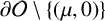
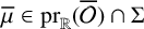
, where
$\overline {\mu }\in \text {pr}_{\mathbb {R}}(\overline {\mathcal {O}})\cap \Sigma $
with
$\overline {\mu }\neq \mu $
.




3 Proof of Theorem 1.1
In view of Proposition 2.5, it is not difficult to verify that problem (2.2) can be equivalently transformed into
 $$ \begin{align*} p=k^2F(p), \end{align*} $$
where the map $F:X\rightarrow X$
is defined by
$F:X\rightarrow X$
is defined by
 $$ \begin{align*} F(p)=\int_\xi^{+\infty}\int_{+\infty}^sgf(p)\,{d}\tau\,{d}s,\quad \xi\geq 0. \end{align*} $$
We claim that F is compact. Assume there is a sequence $p_n$
that weakly converges to some p in X. Without loss of generality, we assume
$p_n$
that weakly converges to some p in X. Without loss of generality, we assume $p=0$
. For any
$p=0$
. For any $\varepsilon>0$
, since
$\varepsilon>0$
, since $p_n$
decays exponentially to
$p_n$
decays exponentially to $0$
at infinity, there exists
$0$
at infinity, there exists $\gamma>0$
such that
$\gamma>0$
such that
 $$ \begin{align*} \bigg\vert\int_\gamma^{+\infty}\int_{+\infty}^sp_n\,{d}\xi\,{d}s\bigg\vert<\frac{\varepsilon}{\max \{1,\alpha^2\}}. \end{align*} $$
It follows that
 $$ \begin{align*} \max \{1,\alpha^2\}\bigg\vert\int_\gamma^{+\infty}\int_{+\infty}^s f(p_n)\,{d}\xi\,{d}s\bigg\vert<\varepsilon. \end{align*} $$
When $\xi>\gamma $
, we have that
$\xi>\gamma $
, we have that
 $$ \begin{align*} \bigg\vert F(p_n)(\xi)\bigg\vert\leq \max\, \{1,\alpha^2\}\bigg\vert\int_\gamma^{+\infty}\int_{+\infty}^s f(p_n)\,{d}\xi\,{d}s\bigg\vert<\varepsilon. \end{align*} $$
While, for $\xi \leq \gamma $
, from the definition of F, we can verify that
$\xi \leq \gamma $
, from the definition of F, we can verify that $F(p_n)\in C^{\alpha }[0,\gamma ]$
with any
$F(p_n)\in C^{\alpha }[0,\gamma ]$
with any $\alpha \in (0,1)$
. Since the embedding
$\alpha \in (0,1)$
. Since the embedding $C^{\alpha }[0,\gamma ]\hookrightarrow C[0,\gamma ]$
is compact,
$C^{\alpha }[0,\gamma ]\hookrightarrow C[0,\gamma ]$
is compact, $F(p_n)$
converges strongly in
$F(p_n)$
converges strongly in $C[0,\gamma ]$
. So, we get that
$C[0,\gamma ]$
. So, we get that $F(p_n)(\xi )\rightarrow 0$
for any
$F(p_n)(\xi )\rightarrow 0$
for any $\xi \leq \gamma $
and n large enough. Therefore, we conclude that
$\xi \leq \gamma $
and n large enough. Therefore, we conclude that $(F(p_n))(\xi )$
converges strongly to
$(F(p_n))(\xi )$
converges strongly to $0$
in X, which verifies the claim. Similarly, it can be proven that F is also continuous. Thus, F is completely continuous.
$0$
in X, which verifies the claim. Similarly, it can be proven that F is also continuous. Thus, F is completely continuous.
Similarly, we define
 $$ \begin{align*} T(p)=\int_\xi^{+\infty}\int_{+\infty}^sg p\,{d}\tau\,{d}s,\quad \xi\geq 0. \end{align*} $$
Reasoning as above, we can still show that $T:X\rightarrow X$
is completely continuous. So,
$T:X\rightarrow X$
is completely continuous. So, $I-k^2 T$
is a completely continuous vector field in X. Thus, the Leray–Schauder degree
$I-k^2 T$
is a completely continuous vector field in X. Thus, the Leray–Schauder degree $\deg (I-\lambda T, B_R(0),0)$
with
$\deg (I-\lambda T, B_R(0),0)$
with $\lambda =k^2$
is well defined for an arbitrary R-ball
$\lambda =k^2$
is well defined for an arbitrary R-ball $B_R(0)$
of X and
$B_R(0)$
of X and $k\in (0,k_2)\setminus \{k_1\}$
.
$k\in (0,k_2)\setminus \{k_1\}$
.
Lemma 3.1. For arbitrary $R>0$
, one has that
$R>0$
, one has that
 $$ \begin{align*} \deg (I-k^2 T, B_R(0),0)= \begin{cases} 1 \quad&\text{if}\ k\in (0,k_1),\\ -1 \quad&\text{if}\ k\in(k_1,k_2). \end{cases} \end{align*} $$
Proof. We only prove the case $k>k_1$
since the proof for
$k>k_1$
since the proof for $k<k_1$
is completely analogous. Since T is compact and linear, by [Reference Deimling6, Theorem 8.10], we have that
$k<k_1$
is completely analogous. Since T is compact and linear, by [Reference Deimling6, Theorem 8.10], we have that
 $$ \begin{align*} \deg (I-k^2 T, B_R(0),0)=-1, \end{align*} $$
which is the desired conclusion.
Now, we can give the proof of our main result.
Proof of Theorem 1.1
In view of Lemma 2.4, problem (2.2) can be written equivalently as
 $$ \begin{align*} p=k^2 T(p)+H(k,p), \end{align*} $$
where
 $$ \begin{align*} H(k,p)=-k^2 \int_\xi^{+\infty}\int_{+\infty}^sg p^2\,{d}\tau\,{d}s. \end{align*} $$
For any $p\in X\setminus \{0\}$
, we have that
$p\in X\setminus \{0\}$
, we have that
 $$ \begin{align} \frac{p^2}{\Vert p\Vert} \leq \frac{\vert p\vert} {\Vert p\Vert}\vert p\vert\leq \Vert p\Vert\rightarrow0\quad \text{as}\ \Vert p\Vert\rightarrow 0. \end{align} $$
Thus, $H(k,p) = o(\Vert p\Vert )$
near
$H(k,p) = o(\Vert p\Vert )$
near $p = 0$
in X uniformly on bounded intervals of k in
$p = 0$
in X uniformly on bounded intervals of k in $(0,+\infty )$
.
$(0,+\infty )$
.
In view of Lemma 3.1, applying Proposition 2.7 by taking $\mathcal {O}=(0,+\infty )\times X$
, we obtain that
$\mathcal {O}=(0,+\infty )\times X$
, we obtain that $(k_1, 0)$
is a bifurcation point of problem (2.2), and the associated bifurcation branch
$(k_1, 0)$
is a bifurcation point of problem (2.2), and the associated bifurcation branch $\mathcal {C}$
in
$\mathcal {C}$
in $(0,+\infty )\times X$
whose closure contains
$(0,+\infty )\times X$
whose closure contains $(k_1, 0)$
satisfies at least one of the following three options: (i) unbounded; (ii) meets to the X at
$(k_1, 0)$
satisfies at least one of the following three options: (i) unbounded; (ii) meets to the X at $k=0$
; (iii) contains a pair
$k=0$
; (iii) contains a pair $(\overline {k}, 0)$
, where
$(\overline {k}, 0)$
, where $\overline {k}$
is an eigenvalue of problem (2.1) and
$\overline {k}$
is an eigenvalue of problem (2.1) and $\overline {k}\neq k_1$
.
$\overline {k}\neq k_1$
.
For any $(k,p)\in \mathcal {C}$
with
$(k,p)\in \mathcal {C}$
with $p\not \equiv 0$
, Lemma 2.4 implies that
$p\not \equiv 0$
, Lemma 2.4 implies that $0<p\leq 1$
in
$0<p\leq 1$
in $[0,+\infty )$
. Hence, we have
$[0,+\infty )$
. Hence, we have $\mathcal {C}\subseteq ((0,+\infty )\times X^+\cup \{(k_1,0)\})$
. We claim that case (ii) does not occur. Assume that
$\mathcal {C}\subseteq ((0,+\infty )\times X^+\cup \{(k_1,0)\})$
. We claim that case (ii) does not occur. Assume that $(k,p)\in \mathcal {C}$
with
$(k,p)\in \mathcal {C}$
with $k\leq k_1$
and
$k\leq k_1$
and $p\not \equiv 0$
. Then, from the argument of Lemma 2.6, we obtain that
$p\not \equiv 0$
. Then, from the argument of Lemma 2.6, we obtain that
 $$ \begin{align*} 0\leq-k_1^2\int_0^{+\infty}gp^2p_1\,{d}\xi<0, \end{align*} $$
which is a contradiction. In fact, we not only proved that the second option does not occur, but we have also proved that the branch $\mathcal {C}$
will not reach the left side of
$\mathcal {C}$
will not reach the left side of $k=k_1$
. That is to say, when
$k=k_1$
. That is to say, when $k\leq k_1$
, problem (1.1) only has the trivial solution
$k\leq k_1$
, problem (1.1) only has the trivial solution $p=0$
.
$p=0$
.
We claim that option (iii) is also impossible. Suppose, in contrast, there exists $(k_n,p_n) \rightarrow (\overline {k},0)$
as
$(k_n,p_n) \rightarrow (\overline {k},0)$
as $n\rightarrow +\infty $
with
$n\rightarrow +\infty $
with $(k_n,p_n)\in \mathcal {C}$
,
$(k_n,p_n)\in \mathcal {C}$
, $p_n \not \equiv 0$
and
$p_n \not \equiv 0$
and $\overline {k}$
is another eigenvalue of problem (2.1). Let
$\overline {k}$
is another eigenvalue of problem (2.1). Let $w_n=p_n/\Vert p_n\Vert $
. Then,
$w_n=p_n/\Vert p_n\Vert $
. Then, $w_n$
satisfies the following problem:
$w_n$
satisfies the following problem:
 $$ \begin{align*} w=k_n^2 T(w)-k_n^2 \int_\xi^{+\infty}\int_{+\infty}^sg wp_n\,{d}\tau\,{d}s. \end{align*} $$
Reasoning as for the compactness of F, we obtain that for some convenient subsequence, $w_n\rightarrow w_0$
as
$w_n\rightarrow w_0$
as $n\rightarrow +\infty $
. From (3.1), we can see that
$n\rightarrow +\infty $
. From (3.1), we can see that $(\overline {k}, w_0)$
verifies problem (2.1) and
$(\overline {k}, w_0)$
verifies problem (2.1) and $\Vert w_0\Vert = 1$
. Since
$\Vert w_0\Vert = 1$
. Since $\mathcal {C}$
does not reach the left side of
$\mathcal {C}$
does not reach the left side of $k=k_1$
, one has that
$k=k_1$
, one has that $\overline {k}>k_1$
. Proposition 2.1 implies that
$\overline {k}>k_1$
. Proposition 2.1 implies that $w_0$
must change its sign, which contradicts the fact that
$w_0$
must change its sign, which contradicts the fact that $p_n>0$
.
$p_n>0$
.
Therefore, the branch $\mathcal {C}$
is unbounded. Moreover,
$\mathcal {C}$
is unbounded. Moreover, $\mathcal {C}$
cannot return to the trivial solution axis and does not reach the left side of
$\mathcal {C}$
cannot return to the trivial solution axis and does not reach the left side of $k=k_1$
. Since
$k=k_1$
. Since $0<p\leq 1$
in
$0<p\leq 1$
in $[0,+\infty )$
for any
$[0,+\infty )$
for any $(k,p)\in \mathcal {C}$
with
$(k,p)\in \mathcal {C}$
with $p\not \equiv 0$
, one sees that
$p\not \equiv 0$
, one sees that $\mathcal {C}$
does not exceed
$\mathcal {C}$
does not exceed $1$
in the X direction. Thus, it must be unbounded in the k direction. Therefore, we obtain that the necessary and sufficient condition for the existence of the cline is
$1$
in the X direction. Thus, it must be unbounded in the k direction. Therefore, we obtain that the necessary and sufficient condition for the existence of the cline is $k>k_1$
.
$k>k_1$
.
We will finally discuss uniqueness and asymptotic behaviour of the cline p. We recall a function defined by Nagylaki [Reference Nagylaki18],
 $$ \begin{align*} T(p_0)=\int_\eta^1\frac{1}{\sqrt{(1-y)\big[1+y-\frac{2}{3}p_0(1+y+y^2)\big]}}\,{d}y, \end{align*} $$
where $\eta =\widetilde {p}_1/p_0$
with
$\eta =\widetilde {p}_1/p_0$
with $\widetilde {p}_1=p(1)$
. Nagylaki proved that
$\widetilde {p}_1=p(1)$
. Nagylaki proved that $T(p_0)$
is strictly increasing to
$T(p_0)$
is strictly increasing to $+\infty $
as
$+\infty $
as $p_0\rightarrow 1^-$
. This implies that there is a unique
$p_0\rightarrow 1^-$
. This implies that there is a unique $p_0$
for
$p_0$
for $k>k_1$
. Reasoning as that of Lemma 2.3 with some obvious changes, we can further show that the uniqueness of
$k>k_1$
. Reasoning as that of Lemma 2.3 with some obvious changes, we can further show that the uniqueness of $p_0$
implies the uniqueness of p. Therefore,
$p_0$
implies the uniqueness of p. Therefore, $\mathcal {C}$
is actually a curve. Moreover, there is a unique cline p for each
$\mathcal {C}$
is actually a curve. Moreover, there is a unique cline p for each $k>k_1$
. The asymptotic behaviour of
$k>k_1$
. The asymptotic behaviour of $T(p_0)$
as
$T(p_0)$
as $p_0\rightarrow 1^-$
implies that
$p_0\rightarrow 1^-$
implies that $\mathcal {C}$
is always less than
$\mathcal {C}$
is always less than $1$
and tends towards
$1$
and tends towards $1$
. This completes the proof of Theorem 1.1.
$1$
. This completes the proof of Theorem 1.1.
4 Proof of Theorem 1.2
In this section, we prove the stability results stated in Theorem 1.2. Define the operator
 $$ \begin{align*} F(k,p)=\frac{p"+k^2g(\xi)p(1-p)}{g(\xi)}. \end{align*} $$
Clearly, the equation of problem (1.1) is equivalent to $-F(k,p)=0$
. Define
$-F(k,p)=0$
. Define
 $$ \begin{align*} Y=\bigg\{p\in X\mid p\in C^2([0,1)\cup(1,+\infty)),\ \lim_{\xi\rightarrow 1^{-}}p"(\xi)\ \text{and}\ \lim_{\xi\rightarrow 1^+}p"(\xi)\ \text{exist}\bigg\}. \end{align*} $$
It is easy to see that the trivial solution $p=0$
belongs to Y and the unique cline p obtained in Theorem 1.1 belongs to Y.
$p=0$
belongs to Y and the unique cline p obtained in Theorem 1.1 belongs to Y.
We recall the stability property of solutions. For any $\phi \in Y$
and positive solution p of problem (1.1), by some simple computations, we can show that the linearized eigenvalue problem of (1.1) about p at the direction
$\phi \in Y$
and positive solution p of problem (1.1), by some simple computations, we can show that the linearized eigenvalue problem of (1.1) about p at the direction $\phi $
is
$\phi $
is
 $$ \begin{align} \begin{cases} -\phi"-k^2g(\xi)(1-2p)\phi=\mu g(\xi)\phi, &\xi>0,\\ \phi'(0)=0, &\lim_{\xi\rightarrow+\infty}\phi'(\xi)=0. \end{cases} \end{align} $$
The linear stability of a solution u of problem (1.1) can be determined by the linearized eigenvalue problem (4.1). A solution p of problem (1.1) is stable if all eigenvalues of problem (4.1) are positive, otherwise it is unstable. Define the Morse index $M(p)$
of a solution p of problem (1.1) to be the number of negative eigenvalues of problem (4.1). A solution p of problem (1.1) is degenerate if
$M(p)$
of a solution p of problem (1.1) to be the number of negative eigenvalues of problem (4.1). A solution p of problem (1.1) is degenerate if $0$
is an eigenvalue of problem (4.1), otherwise it is nondegenerate.
$0$
is an eigenvalue of problem (4.1), otherwise it is nondegenerate.
Now, we can present the argument of Theorem 1.2.
Proof of Theorem 1.2
We first study the stability of the nontrivial solution. Let $(k_*, p_*)$
be a nontrivial solution of (1.1). The Fréchet derivative of F with respect to p at
$(k_*, p_*)$
be a nontrivial solution of (1.1). The Fréchet derivative of F with respect to p at $(k_*, p_*)$
is given by
$(k_*, p_*)$
is given by
 $$ \begin{align*} F_p(k_*, p_*)\varphi = \frac{\varphi" + k_*^2g(\xi)(1-2p_*)\varphi}{g(\xi)}, \quad \varphi \in Y. \end{align*} $$
Let $\mu _1$
be the first eigenvalue of the operator
$\mu _1$
be the first eigenvalue of the operator $-F_p(k_*, p_*)$
.
$-F_p(k_*, p_*)$
.
We claim that the corresponding eigenfunction $\varphi _1$
is positive. Note that
$\varphi _1$
is positive. Note that $\varphi _1$
satisfies
$\varphi _1$
satisfies
 $$ \begin{align} -\varphi_1"-k_*^2g(\xi)(1-2p_*)\varphi_1=\mu_1g(\xi)\varphi_1. \end{align} $$
We claim that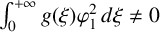 $\int _0^{+\infty }g(\xi )\varphi _1^2\,{d}\xi \neq 0$
. Indeed, if it was, we obtain from (4.2) that
$\int _0^{+\infty }g(\xi )\varphi _1^2\,{d}\xi \neq 0$
. Indeed, if it was, we obtain from (4.2) that
 $$ \begin{align*} \int_0^{+\infty} \varphi_1^{\prime2}\,{d}\xi+2k_\ast^2\int_0^{+\infty} g(\xi)\varphi_1^2 p_\ast\, {d}\xi=0. \end{align*} $$
This implies
 $$ \begin{align*} \int_0^{+\infty} g(\xi)\varphi_1^2 p_*\, {d}\xi<0. \end{align*} $$
So, we have
 $$ \begin{align*} \int_0^{1} \varphi_1^2 p_*\, {d}\xi<\alpha^2\int_1^{+\infty} \varphi_1^2 p_*\, {d}\xi. \end{align*} $$
Using the monotonicity of $p_*$
, we see that
$p_*$
, we see that
 $$ \begin{align*} \alpha^2 p_*(1) \int_1^{+\infty} \varphi_1^2 \, {d}\xi &= p_*(1) \int_0^{1} \varphi_1^2 \, {d}\xi \\ &\leq \int_0^{1} \varphi_1^2 p_* \, {d}\xi \\ &< \alpha^2 \int_1^{+\infty} \varphi_1^2 p_* \, {d}\xi \\ &\leq \alpha^2 p_*(1) \int_1^{+\infty} \varphi_1^2 \, {d}\xi, \end{align*} $$
which is a contradiction. Hence, we have the following Rayleigh quotient of $\mu _1$
:
$\mu _1$
:
 $$ \begin{align*} \mu_1=\inf_{u\in Y\setminus\{0\}} \frac{\int_0^{+\infty} \varphi_1^{\prime2}\,{d}\xi-k_\ast^2\int_0^{+\infty}g(\xi)(1-2p_\ast)\varphi_1^2\,{d}\xi}{\int_0^{+\infty}g(\xi)\varphi_1^2\,{d}\xi}. \end{align*} $$
It follows that $\vert \varphi _1\vert $
is also the eigenfunction corresponding to
$\vert \varphi _1\vert $
is also the eigenfunction corresponding to $\mu _1$
. Since
$\mu _1$
. Since $\varphi _1$
is in
$\varphi _1$
is in $C^1$
, we further obtain that
$C^1$
, we further obtain that $\varphi _1$
has only one sign. Without loss of generality, we assume that
$\varphi _1$
has only one sign. Without loss of generality, we assume that $\varphi _1$
is nonnegative. If
$\varphi _1$
is nonnegative. If $\varphi _1$
has a zero
$\varphi _1$
has a zero $\xi _0>0$
which clearly is a double zero, by an argument similar to that of Lemma 2.3 with obvious changes, we can show that
$\xi _0>0$
which clearly is a double zero, by an argument similar to that of Lemma 2.3 with obvious changes, we can show that $\varphi _1\equiv 0$
, which is impossible. Thus, we conclude that
$\varphi _1\equiv 0$
, which is impossible. Thus, we conclude that $\varphi _1$
is positive.
$\varphi _1$
is positive.
Since $k_*$
and
$k_*$
and $p_*$
are a solution of (1.1), we have
$p_*$
are a solution of (1.1), we have
 $$ \begin{align} -p_*"-k_*^2g(\xi)p_*(1-p_*)=0. \end{align} $$
Multiplying (4.2) by $p_*/g(\xi )$
and (4.3) by
$p_*/g(\xi )$
and (4.3) by $\varphi _1/g(\xi )$
, subtracting the resulting equations and integrating over
$\varphi _1/g(\xi )$
, subtracting the resulting equations and integrating over $[0, +\infty )$
, we obtain, after integration by parts,
$[0, +\infty )$
, we obtain, after integration by parts,
 $$ \begin{align*} \mu_1\int_0^{+\infty} \varphi_1 p_* {d}\xi = k_*^2\int_0^{+\infty} \varphi_1 p_*^2\, {d}\xi. \end{align*} $$
Since both integrands are positive, it follows that $\mu _1> 0$
. Consequently, all eigenvalues of
$\mu _1> 0$
. Consequently, all eigenvalues of $-F_p(k_*, p_*)$
are positive. Thus, for any
$-F_p(k_*, p_*)$
are positive. Thus, for any $k>\arctan \alpha $
, the cline p is (asymptotically linearly) stable.
$k>\arctan \alpha $
, the cline p is (asymptotically linearly) stable.
Next, we investigate the stability of the trivial solution $p=0$
. Set
$p=0$
. Set $p(s)=0$
and
$p(s)=0$
and $k(s)=k_1+s$
for
$k(s)=k_1+s$
for $s\in \mathbb {R}$
and
$s\in \mathbb {R}$
and $s>-k_1$
. The Fréchet derivative of F with respect to p at
$s>-k_1$
. The Fréchet derivative of F with respect to p at $(k(s),p(s))$
is given by
$(k(s),p(s))$
is given by
 $$ \begin{align*} F_p(k(s),p(s))\varphi(s)=\frac{\varphi"(s)+k^2(s)g(\xi)\varphi(s)}{g(\xi)}\quad \text{for all } \varphi(s)\in Y. \end{align*} $$
We assume that the first eigenvalue of $-F_p(k(s),p(s))$
is
$-F_p(k(s),p(s))$
is $\mu (s)$
with the corresponding eigenfunction
$\mu (s)$
with the corresponding eigenfunction $\phi (s)$
. Then,
$\phi (s)$
. Then, $\phi (s)$
satisfies
$\phi (s)$
satisfies
 $$ \begin{align} -\phi"(s)-k^2(s)g(\xi)\phi(s)=\mu(s)g(\xi)\phi(s). \end{align} $$
As in the above case, we still can show that $\phi (s)$
is positive. From the spectral analysis in Section 2, we recall that when
$\phi (s)$
is positive. From the spectral analysis in Section 2, we recall that when $k(s) = k_1$
, (4.4) has a zero eigenvalue. A direct computation shows that for
$k(s) = k_1$
, (4.4) has a zero eigenvalue. A direct computation shows that for $k(s) \neq k_1$
, the first eigenvalue is given by
$k(s) \neq k_1$
, the first eigenvalue is given by
 $$ \begin{align*} \mu(s)=k_{1}^{2}-k^2(s)= \begin{cases}>0, &s<0,\\ <0, &s>0. \end{cases} \end{align*} $$
It follows that $p=0$
is (asymptotically linearly) stable when
$p=0$
is (asymptotically linearly) stable when $s<0$
and unstable when
$s<0$
and unstable when $s>0$
. This completes the proof of Theorem 1.2.
$s>0$
. This completes the proof of Theorem 1.2.
From the argument of Theorem 1.2, we know that the cline p is nondegenerate and has Morse index $M(p)=0$
. The trivial solution
$M(p)=0$
. The trivial solution $p=0$
is nondegenerate and has Morse index
$p=0$
is nondegenerate and has Morse index $M(0)=0$
for
$M(0)=0$
for $k<k_1$
.
$k<k_1$
.
5 Conclusion
In this paper, we have shown that for a semi-infinite habitat with a piecewise-constant sign-changing selection coefficient, there exists a unique cline if and only if $k> \arctan \alpha $
. The bifurcation branch emanating from
$k> \arctan \alpha $
. The bifurcation branch emanating from $(k_1,0)$
is unbounded and tends to
$(k_1,0)$
is unbounded and tends to $1$
as
$1$
as $k\to +\infty $
. Moreover, every cline on this branch is asymptotically linearly stable, while the trivial solution
$k\to +\infty $
. Moreover, every cline on this branch is asymptotically linearly stable, while the trivial solution $p=0$
is stable for
$p=0$
is stable for $k<k_1$
and unstable for
$k<k_1$
and unstable for $k>k_1$
. These results give a complete affirmative answer to Nagylaki’s conjecture and provide a rigorous mathematical foundation for cline models in population genetics.
$k>k_1$
. These results give a complete affirmative answer to Nagylaki’s conjecture and provide a rigorous mathematical foundation for cline models in population genetics.
Acknowledgement
This research was supported by NNSF of China (No. 12371110).