


INTRODUCTION
Pressure ridges are one of the most dominant topographical surface features of the sea-ice cover. These structural deformations in the sea ice are created by the interaction or pressure between separate ice floes as they move toward or past each other and collide (Parmerter and Coon, Reference Parmerter and Coon1972). They are of climatological interest due to their impact on the mass, energy and momentum transfer of the polar oceans (Wittman and Schule, Reference Wittman, Schule and Fletcher1966; Arya, Reference Arya1973; Martin, Reference Martin2007) and are important to those operating in ice-infested waters since they form a barrier to travel (Kovacs and others, Reference Kovacs, Weeks, Ackley and Hibler1973). Understanding the regional and seasonal distribution of ridges, and their variability is important for quantifying total sea-ice mass and for improving the treatment of sea-ice dynamics in high-resolution numerical models.
Pressure ridges are described mathematically with a variety of parameters including sail height, keel draft and sail and keel width (Kovacs and others, Reference Kovacs, Weeks, Ackley and Hibler1973). Sail height describes the raised part of the ridge above the local sea-ice surface and depends on the thickness of the parent ice floe (Parmerter and Coon, Reference Parmerter and Coon1972). The keel draft describes the depth of the ice that is forced down vertically by compressive stresses during the collision of ice floes. Like sail height, keel draft depends on the thickness of the parent ice floe and can be related to the sail height through a draft:sail height ratio. Previous studies have shown that ridge draft is approximately five to six times larger than sail height (Martin, Reference Martin2007). Sail and keel width can vary greatly, however. Typically keel width is approximately five times larger than sail width (Evers and Jochmann, Reference Evers and Jochmann1998).
Sail height is related to both the energy required to form the pressure ridge, as well as the thickness of the parent sea-ice sheet (Rothrock, Reference Rothrock1975). Hence measurements of sail height can provide information about the strength of the parent ice sheet forming the ridge. Pressure ridge sails present a form drag for air moving over the rough sea-ice surface (Arya, Reference Arya1973; Castellani and others, Reference Castellani, Lupkes, Hendricks and Gerdes2014; Tsamados and others, Reference Tsamados2014). Increasing the quality and quantity of sail height measurements will enable estimation of variability in ridge parameters and lead to improved representation in sea-ice models.
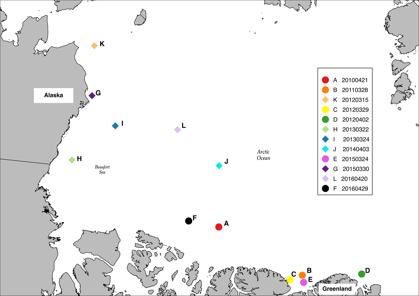
Ridges are easy to visually observe, making it possible to measure sail height both in situ (e.g. Kovacs and others, Reference Kovacs, Weeks, Ackley and Hibler1973) and from airborne platforms (e.g. Mock and others, Reference Mock, Hartwell and Hibler1972; Hibler and others, Reference Hibler, Mock and Tucker1974; Hibler and Ackley, Reference Hibler and Ackley1975; Wadhams, Reference Wadhams1981). Previous studies have measured the shadows cast by pressure ridges to derive sail height in the Western Arctic (Hibler and Ackley, Reference Hibler and Ackley1975) and in the marginal ice zone (Miao and others, Reference Miao, Xie, Ackley and Zheng2016), but these techniques have yet to be applied across the basin scale or validated with independent height measurements. Building on this previous work, we present a new methodology to identify and map shadows cast by pressure ridges in high-resolution Digital Mapping System (DMS) imagery, obtained from an airborne platform. We relate shadow length to sail height. The methodology is tested by deriving the full sail height distribution along the length of 12, newly formed pressure ridges, located across the western and central Arctic Ocean (Fig. 1). Unique to this study, sail heights derived from DMS imagery, are evaluated through comparison with spatially coincident measurements of surface elevation obtained by an airborne laser altimeter, the Airborne Topographic Mapper (ATM). We assess the sail height distribution and the sail height profile of the pressure ridge along its long axis in the context of ATM elevations, and we compute their correlation. Of the ridges examined, we compare sail height characteristics of ridges that formed in regions of first-year ice (FYI) with those that formed in multi-year ice (MYI) areas. We seek to provide a proof of concept for the utility of DMS imagery to characterize pressure ridge sail height, prior to initiating a further study of the full suite of available DMS imagery.
Map of the Arctic Ocean outlining the location of 12 pressure ridges examined in this study. All are new pressure ridges formed in areas dominated by first year (diamonds) or multi-year ice (circles).
INSTRUMENTATION
The NASA's Operation IceBridge (OIB) airborne mission now performs annual surveys of the Arctic sea-ice cover. These missions present a new opportunity to conduct detailed investigations of sea-ice surface morphology over an extended observation period. OIB was initiated in 2009 (Koenig and others, Reference Koenig, Martin, Studinger and Sonntag2010) with the goal to bridge the gap between observations from the original ICESat mission, decommissioned in 2009, and the ICESat-2 mission, scheduled for launch in 2018. An Arctic OIB campaign is flown annually during the late winter months of March, April and May and has provided consistent data collection over long transects of the western and central Arctic for the past 9 years. During these campaigns, airborne remote sensing measurements over sea ice are collected by a variety of instruments, including laser altimeters, a snow radar, a Ku-band radar and digital camera systems. This unique, multi-sensor dataset enables coincident measurements from different instruments to be directly compared and combined. In this study, we utilize data collected by two OIB instruments during the annual Arctic Spring campaigns of 2010–2016: the DMS digital camera and the ATM laser altimeter.
DMS
The DMS was first added to the OIB instrument suite for Arctic studies in 2010. DMS images have been widely used for lead detection (e.g. Farrell and others, Reference Farrell, Kurtz, Onana, Harbeck and Duncan2011; Onana and others, Reference Onana2013) and to characterize sastrugi and other features of snow on sea ice (Newman and others, Reference Newman2014). The DMS is a nadir-facing digital camera that provides high-resolution imagery. Assuming a nominal flight altitude of 450 m, each DMS image represents an area ~650 × 420 m on the Earth's surface, with a spatial (pixel) resolution of ~0.1 m. The images have been geolocated and orthorectified with the use of an Applanix POS/AV orientation system. In this study, we utilize the geolocated and orthorectified level-1B (IODMS1B) DMS geotiff dataset (Dominguez, Reference Dominguez2016).
ATM
The ATM laser altimeters (Krabill and others, Reference Krabill2002) on OIB have provided high-resolution measurements of sea-ice surface topography since 2009. ATM elevation data can be used to detect surface features such as leads between sea-ice floes (e.g. Connor and others, Reference Connor, Farrell, McAdoo, Krabill and Manizade2013) as well as combined with snow radar data and DMS visible imagery, to derive sea-ice freeboard and thickness (e.g. Farrell and others, Reference Farrell2012; Kurtz and others, Reference Kurtz2013; Richter-Menge and Farrell, Reference Richter-Menge and Farrell2013).
The ATM is a conically scanning laser altimeter that operates at a wavelength of 532 nm. When flown at the nominal altitude of 450 m, the ATM lidar system generates a 1 m footprint on the sea-ice surface, with variable along-track spacing between laser pulses, ~5 m on average. Due to the scanning geometry, the density of footprints on the sea-ice surface is nonuniform with a higher (lower) density at the swath edges (center). The ATM may be operated in a wide-scan or narrow-scan configuration. The scan angle of the narrow-scan instrument is ~2.7°, which at a nominal altitude yields a swath width of ~45 m. The scan angle of the wide-scan instrument is typically 15° and yields a swath width of ~250 m. Often, two ATM instruments are flown contemporaneously to exploit both swath widths, wherein the narrow-scan configuration increases sampling at the center of the wide-scan swath. In this study, we utilize the ATM Level-1B Elevation and Return Strength (ILATM1B) wide-scan dataset collected during the Arctic campaigns of 2010–16 and the Level-1B Elevation and Return Strength (ILNSA1B) narrow-scan data from 2011–16 (Studinger, Reference Studinger2017a, Reference Studingerb).
Sensor Sampling
The conical scanning mode of the ATM laser altimeter results in uneven sampling across the sea-ice surface (illustrated by blue and green dots in Figs 2a and c). Moreover, the wide-scan and narrow-scan ATM instrument configurations each produce a different sampling density (ATM footprints/m) in the across-swath/across-track direction. So, over the highly variable sea-ice surface topography (due to features including snow dunes, sastrugi, pressure ridge sails, rubble fields and leads) the ATM preferentially samples morphological features depending on their location relative to the ATM swath, with many more ATM footprints at the swath edges than at the center. Consider a pressure ridge oriented parallel to the direction of flight (i.e. along-track) and positioned at the center of the ATM wide-scan swath (Fig. 2a). In this configuration, the sampling density of ATM wide-scan over the ridged ice is ~0.28 m−1, while the sampling density of the ATM narrow-scan is ~2.3 m−1 (Fig. 2b). Now consider a ridge oriented perpendicular to the direction of flight, in the across-track direction (Fig. 2c). In this configuration the sampling density of the ATM wide-scan over the ridged ice averages ~0.35 m−1, but sampling density increases to ~2 m−1at either end of the ridge where many ATM footprints overlap at the edges of the ATM swath (Fig. 2d). The sampling density of the ATM narrow-scan over the ridge is ~2 m−1, however, only one short section (~45 m long) of the pressure ridge is sampled (Fig. 2d).
ATM wide-scan (blue dots), and ATM narrow-scan footprints (green dots) overlaid on a DMS image of sea ice pressure ridge oriented in (a) the along-track direction and (c) the across-track direction. DMS pixels along the ridge crest are identified with black dots. (b) Sampling density for each sensor, given in terms of ATM footprints m−1 or DMS pixels m−1, along the pressure ridge oriented in (b) the along-track direction and (d) the across-track direction.
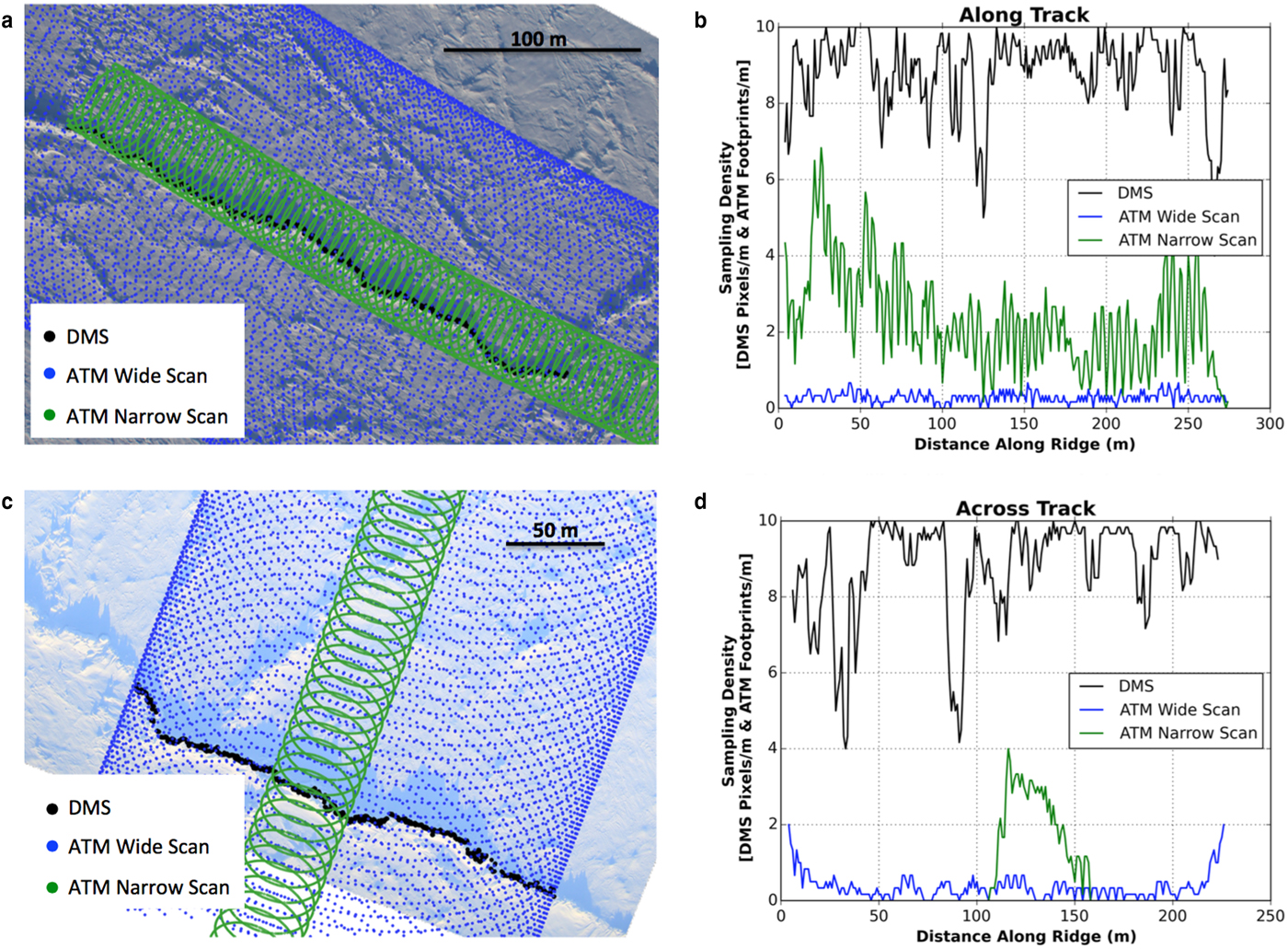
The DMS, on the other hand, provides continuous and uniform sampling across the sea-ice surface in both the along- and across-track directions, such that ridge orientation does not impact measurement density (pixels m−1). For both pressure ridge configurations (along- and across-track), the DMS sample density averaged ~8.8 m−1 (Figs 2b and d).
As a consequence of the uneven ATM sampling, in many cases, the ATM does not provide enough elevation measurements of a pressure ridge to evaluate the DMS-derived sail height. This has implications for the choice of pressure ridge selected for our study. For example, the ATM sample density illustrated in Figure 2c and d does not provide sufficient measurements of ridge elevation and thus this pressure ridge cannot be used for cross-comparison of ATM elevations and DMS-derived sail height measurements. Conversely, the pressure ridge shown in Figure 2a and b is a reasonable candidate for our study, since the combined ATM wide- and narrow-scans provide adequate sampling of sail elevation.
METHODOLOGY
Selection of ridges for evaluation
The goal of our study is to demonstrate that pressure ridge sail height can be extracted from DMS images. To determine the utility of the DMS data, and demonstrate our methodology, sail heights are evaluated via comparison with spatially coincident ATM elevation measurements. For this specific evaluation, we therefore require that the pressure ridge is tracked in both the ATM and DMS datasets. This requirement results in three constraints on the ridges examined in our study. First, the ridge must not fall outside of the ATM wide-scan swath. Second, to maximize ATM sampling along the ridge crest, it is preferable that the ridge is oriented close to the along-track flight direction. Third, pressure ridge length must be considered so as to obtain a large enough sample of ATM elevations along each ridge crest. Taken together, these requirements limit the availability of suitable pressure ridges for evaluation of sail height. Thus, the 12 pressure ridges studied here were selected based on both their orientation (relative to the direction of flight) and their length, to ensure optimal ATM sampling along the ridge.
The ridges selected were distinct and usually solitary, with minimal obstruction by intersecting ridges or rubble (Fig. S1). The examples span a variety of geographic locations in the central and western Arctic (Fig. 1). Samples span an observation period between 2010 and 2016, with at least one ridge per OIB Spring campaign. All are examples of new ridges (World Meteorological Organization, 1970) evident from their blocky appearance with sharp peaks. New ridges, also referred to as first-year ridges (Tucker and Govoni, Reference Tucker and Govoni1981), have formed since the preceding melt season, and differ from weathered or aged ridges that exhibit a more rounded appearance. Figure S1 indicates the blocky appearance of these new ridges, as well as the ridge setting which provides some evidence of the ice type from which the ridge formed. To further understand the regional setting of the samples, we also examined satellite-derived ice-type products, including those available at http://www.scp.byu.edu/data/Ascat/iceage/ASCAT_MYFY.html and http://osisaf.met.no/p/ice/. These products exploit differences in the radar backscatter and microwave emissions between FYI and MYI as measured by the Advanced Scatterometer (ASCAT) and the passive microwave radiometer on the Special Sensor Microwave Imager/Sounder (SSMIS), respectively, to identify ice type across the Arctic (e.g. Lindell and Long, Reference Lindell and Long2016). This information was used to estimate the regional setting of the sampled ridges. The 12 examples used in this study are located in regions of predominantly FYI in the Canada Basin (Fig. 1, diamonds) and predominantly MYI in the central Arctic (Fig. 1, dots).
DMS sail height
Dark shadows cast by pressure ridge sails are distinct from the bright sea-ice surface and are thus easy to identify in DMS images (Fig. S1). We exploit this in our methodology to identify and map shadows cast by ridge sails and then to relate the length of the shadow to sail height. We have developed a fully automatic process to identify the shadows cast by ridge sails. First, we discard pixels with a brightness value of 0. These pixels are associated with the black border surrounding each DMS image that is used to fully contain each image within the geotiff array and mitigate against the impact of aircraft pitch, roll and/or altitude variations. Also, pixel artifacts with brightness values ranging from 1 to 7 occur along the edge between the black border and the image as a result of image compression. These pixels are also discarded. Thus, in the subsequent steps, only pixels with brightness values greater than or equal to 8 are considered.
DMS images are provided in a red-green-blue (RGB) format. The red-band component (Fig. 3a) is utilized since it provides greater contrast between sea-ice floes and ridge sail shadows, than the green and blue bands. A histogram of pixel brightness is calculated for the red-band image (Fig. 3b) as an initial attempt to distinguish modes associated with sail shadows and ice floes. However, if the ratio of pixels occupied by sail shadows to those occupied by ice floes is low, the histogram will be unimodal, as illustrated in Figure 3b. In this case, pixels are tested against a set of low pixel brightness ranges. The pixel brightness in DMS images is variable across the OIB Arctic campaigns and can even vary during a single flight survey due to changing cloud conditions and sun elevation angle. Therefore, varying pixel brightness ranges are used to detect shadows cast by pressure ridge sails within each DMS image. This approach, versus using a single, fixed pixel brightness threshold, allows for the detection of ridge sail shadows across a larger number of images. Initially, a range of pixel brightness values between 30 and 100 is used. Of the pixels identified in the initial test, the location of one pixel is selected randomly. All pixels in a 600 × 600 pixel box surrounding the randomly selected pixel (red box, Fig. 3a) define a subset of the original image (Fig. 3c), where shadows may be prominent. A histogram of pixel brightness values is calculated using the data in the subset image (Fig. 3d) and, if the ratio of shadow to floe pixels is high, then the histogram has a bimodal shape. If the histogram is unimodal, the test is repeated using a different range of pixel brightness values, until a bimodal histogram is found, or the test fails and no sail shadows are identified. The test is conducted up to five times, over the following additional pixel brightness ranges: 60–85, 85–105, 120–150, 100–170.
Diagram depicting the methodology applied to the DMS visible images. (a) Red spectral band of original RGB DMS image. (b) Histogram of pixel brightness for red spectral band of the DMS image. (c) Image subset (indicated by red box in a). (d) Histogram of pixel brightness for the subsetted image (shown in c). β indicates the minimum value between the two modes (e) Binary image mask (black pixels are shadows; white pixels are floes) of red spectral band image. (f) Rotated binary image mask used in sail height calculation. (g) Diagram depicting the relevant angles for the rotation of the DMS image.
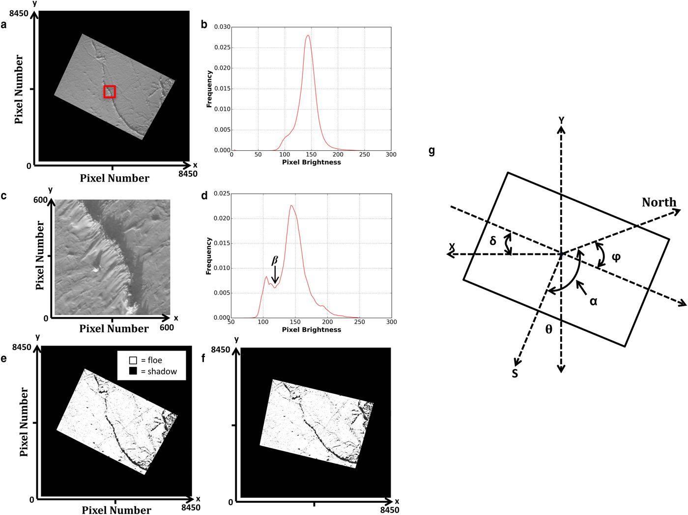
Upon obtaining a bimodal pixel brightness histogram, the mode associated with sail shadows may be distinguished from the mode associated with sea-ice floes. The minimum point between the two modes (β, Fig. 3d) is found. All pixel brightness values between 8 and the value β are thus defined as sail shadow pixels. This range is applied to the full red-band DMS image creating a binary mask distinguishing between sail shadow and ice floe pixels (Fig. 3e). In the following section, we describe the steps that are taken to rotate the image (Fig. 3f), to allow sail height to be derived automatically from the length of the sail shadows.
Metadata delivered with the DMS images provide the pixel resolution of each image (which varies depending on aircraft altitude). The metadata also provide the acquisition time, date, and central latitude, ω, and longitude, λ, of each image, as well as the pitch, roll and altitude of the aircraft. In order to accurately count the sail shadow pixels and measure the sail height in each image mask, the images must be rotated so that sail shadows are vertically oriented along the y-axis of a Cartesian grid with the center latitude and longitude of the masked image at the origin (Fig. 3f).
Figure 3g depicts the relevant angles required for accurate rotation of the DMS image. The rotation angle, θ, is found by combining knowledge of the horizontal flight direction angle, δ, the solar azimuth angle α and the true heading angle, φ:
 $$\theta {\rm \;} = 90\; - \; \left( {180\; - \; \left( {\alpha {\rm \;} - {\rm \;}} \varphi \right)\; + \; \delta} \right)$$
The horizontal flight direction angle, δ, describes the deviation of the image from the x-axis with respect to the flight direction. The angle δ is found by using two corner points of the image, one at the lower left corner (P1) and a second at the lower right corner (P2), as follows:
 $$\delta = \tan ^{ - 1}\left( {\displaystyle{{P2_{y\;} - \; P1_y} \over {P2_x - \; P1_x}}} \right)$$
The true heading angle, φ, is obtained from navigation files (provided for each OIB flight) and describes the angular direction of the aircraft with respect to true north (i.e., at a latitude/longitude of 90, 0). Eqn 1 is used to rotate the image so that the solar radiation (S, Fig. 3g) will be aligned along the y-axis, simplifying the calculation of sail height.
The solar azimuth angle α is calculated using the following steps. First, the day and month of image acquisition is converted to the day of the year, N, with a provision for leap years in 2012 and 2016 so as to include 29 February. N is used to resolve the local apparent time, τ, in minutes, as shown in Eqn (3). Eqn 3 is an approximation, with the first term correcting for the obliquity of the Earth's orbit and the second and third terms correcting for the eccentricity.
 $$\tau \; = 9.87\sin 2B - 7.53\cos B - 1.5\sin B$$
where B = 360/365 × (N − 81). Next, the local standard time meridian, Ω, is established using the longitude, λ. Ω is a reference meridian used to establish “time zones” which occur longitudinally every 15° from the Prime Meridian. Ω and λ are used in conjunction with τ to calculate a net time correction, ε, in minutes:
 $$\epsilon \; = (4\; \times \; \left( {{\rm \lambda} - \; {\rm \Omega}} \right)) + \tau $$
The first term in ε accounts for the variation of the local time within a given 15° time zone due to differences in longitude. Using ε, the time of image acquisition (as, hour I h and minutes I m) is adjusted to reflect the local solar time, γ. γ represents the corrected image acquisition time, in hours, based on the longitude at which the image was acquired:
 $$\gamma \; = \left( {I_{\rm h}\; - \; \left( {\displaystyle{{\rm \Omega} \over {15}}} \right)} \right) + \; \displaystyle{{I_{\rm m}} \over {60}} + \displaystyle{\epsilon \over {60}}$$
Next, solar hour angle, η, and declination angle, χ, are calculated:
 $$\eta \; = \left( {\gamma - 12} \right)\; \times \; 15$$
 $$\eqalign{\chi & = - {\rm sin}^{ - 1}[0.39779 {\rm cos} (0.98565 (N + 10) \cr & + 1.914 {\rm sin} (0.98565(N - 2)))}]$$
where the constant 0.39779 represents the Earth's obliquity (sin (23.44)), the constant 0.98565 represents the number of degrees in one revolution divided by the total number of days in a year (360/365.25), and the constant 1.914 represents the eccentricity of Earth's orbit ((360/π) × 0.0167).
Now the solar elevation angle, a, and azimuth angle, α, may be calculated:
 $$a\; = \sin ^{ - 1}[(\sin \chi \; \times \; \sin {\rm \omega} ) + (\cos \chi \; \times \; \cos {\rm \omega} \; \times \; \cos \eta )]$$
 $$\alpha = \cos ^{ - 1}\left[ {\displaystyle{{((\sin \chi \; \times \; \cos {\rm \omega} ) - (\cos \chi \; \times \; \sin {\rm \omega} \; \times \; \cos \eta ))} \over {\cos a}}} \right]$$
Now that all of the relevant angles are defined, the binary DMS image mask may be rotated. Rotation results in sail shadows that are vertically oriented along the y-axis of the Cartesian grid (Fig. 3f). The mask is scanned in a column-wise direction (top to bottom, left to right) to identify and calculate the length of individual sail shadow segments. Sail shadow segments start when a shadow pixel is encountered after a floe pixel and continue until the next floe pixel is encountered. Sail shadow segments are thus identified and the number of pixels in each segment is multiplied by the pixel size of that specific image to obtain shadow length, ℓ, measured in meters. Following Hibler and Ackley (Reference Hibler and Ackley1975), sail height, H s, is defined as
 $$H_{\rm s} = \ell {\rm \;} \times {\rm \;} \tan a$$
where a is the solar elevation angle, defined earlier in Eqn 8. The precision of H S is ~0.1 m, based on the approximate pixel resolution of the DMS images. Tan and others (Reference Tan, Li, Lu, Haas and Nicolaus2012) found that 0.62 m was an optimal cut-off height to separate pressure ridges from other sea-ice surface undulations. Following Tan and others (Reference Tan, Li, Lu, Haas and Nicolaus2012) and confirmed here by visual inspection, minimum sail height is set to 0.6 m, so as to exclude any measurements of shadows cast by sastrugi or other small topographic features on the sea-ice surface.
ATM surface elevation anomaly
ATM measures surface height, H, with respect to the WGS84 reference ellipsoid with a shot-to-shot precision of ~0.05 m over a level sea-ice surface (Farrell and others, Reference Farrell2012). Here we define a surface elevation anomaly, H A, which is the height H above the local level ice surface, H L. The local level ice surface, H L, is a confined area of smooth ice/snow located within the bounds of the DMS image, and within the vicinity of the pressure ridge. H L is defined as any area where the Std dev. of H is <0.07 m, thereby indicating an area of smooth ice/snow. H L is computed by averaging no fewer than 300 ATM measurements. Thus, the elevation anomaly, defined as, H A = H −H L, is the ATM elevation with respect to the local level ice surface. H A is a useful metric for direct comparison with sail height, H S, since it is an alternative measurement of height above the local level ice surface. Further, it is computed independently of the parameters used to calculate H S. H A is used here to evaluate the accuracy of H S.
RESULTS
ATM elevation anomalies (H A) and DMS sail heights (H S) were extracted for 12 pressure ridges located across the Arctic Ocean (Fig. 1). H A measurements within a 1 m radius of the ridge crest were extracted where ATM and DMS datasets overlapped. Details including the date of measurement, geographic location of the ridge and the predominant ice-type are presented in Table 1. Pressure ridges ranged in length from 97 to 411 m, with only two ridges <200 m long (Table 1). The number of independent measurements of H S and H A per ridge differed by an order of magnitude; DMS provided an average of ~2200 H S measurements, while ATM provided an average of ~280 H A measurements.
Distributions of DMS sail height (black) and ATM surface elevation anomalies (red) for 12 pressure ridges. Histogram bin width is 0.1 m.

Statistics describing 12 pressure ridge sails (A−L). Number of measurements, mean, mode and maximum refer to distributions shown in Figure 4

* ATM wide scan only.
† ATM wide and narrow scan.
Mean and modal H S ranged from 1.08 to 2.16 m and 0.6 to 2.0 m, respectively, while mean and modal H A ranged from 0.99 to 2.13 m and 0.6 to 2.4 m, respectively (Table 1). On average mean H S and H A agree to within 0.11 m. Ridge E is the outlier, where a mean height difference of 0.39 m is observed, although this is also the shortest ridge with a limited availability of ATM measurements (Table 1). Maximum H S ranged from 2.1 to 4.8 m, while maximum H A ranged from 1.9 to 5.4 m. For nine of the 12 ridges (A, B, D, E, G-K) the maximum values of H S and H A agree to within 0.5 m or better. However, for ridge C the maximum H A was 1.0 m higher than the maximum H S. This is likely due to an obstruction of the sail shadow causing an underestimate of H S at that particular location along the ridge. On the other hand, for ridges F and L the maximum H A was 1.0–1.2 m lower than the maximum HS. This is likely due to ATM sampling, where footprints were located on the flanks rather than on the crests of these ridges.
Sail height distributions
The full sail height distribution was derived from DMS imagery for each pressure ridge and compared with the independent and coincident, distributions of surface elevation anomaly derived from the ATM (Fig. 4). In the majority of cases, the distributions for H S and H A overlap and there is an excellent agreement between the two datasets (Fig. 4). Ridge E (the shortest ridge) is again the exception, where the distribution of H A is biased low compared with that of H S.
The results may also be considered in the context of the predominant ice type observed in the area of ridge formation and inspection of Figure 4 suggests that the sail height distribution is related to the surrounding ice type. The distributions indicate that the sail heights of ridges developed in areas that were predominantly MYI (A−F) are approximately double those that developed in regions that were predominantly FYI (G−L). Indeed, of the ridges examined, Table 1 shows that both mean and maximum H S was over 50% larger for ridges that formed in regions dominated by MYI than those that formed in regions dominated by FYI. The H S distributions for ridges formed in areas of predominantly MYI have a broader shape and a larger range of sail heights than those that developed in areas of predominantly FYI (Fig. 4). Modal H S (defined using a bin-width of 0.1 m) also differed by ice type (Table 1), ranging from 0.7 to 2.0 m (and averaging 1.5 m) for ridges in a MYI setting, compared with 0.6–1.8 m (and averaging 0.9 m) for ridges in a FYI setting.
Sail height profiles
Next, we inspect the along-track profiles of H S and H A for each ridge (Figs 5a and b) to examine correspondence between the DMS and ATM measurements along ridge crests. The origin of the ridge where both datasets first overlap (distance = 0) was established at either the lowest or highest longitude value, depending on flight direction. As indicated in Table 1, the total number of DMS measurements along each ridge averages ~11 times that of the ATM, due to differences in the sampling density of the two sensors. Moreover, as demonstrated in Figure 2, measurements of H A may arise from either the crest or flanks of the pressure ridge sail. Figures 5a and b show the full-resolution H S (grey crosses) and H A (pink crosses) measurements and demonstrates that the DMS delivers a higher-fidelity observation of the detailed sail-height profile than the ATM lidars.
(a) DMS sail heights (grey crosses) and ATM elevation anomalies (pink crosses) for ridges A−F. DMS and ATM measurements, resampled at 1 m resolution, are also shown (black and red lines, respectively). Light blue shading indicates the location of narrow-scan ATM coverage along the pressure ridge. Blue arrows indicate instances where the location of the maximum DMS sail height and ATM elevation are offset. Green arrows indicate examples where the sail height is lower than the ATM elevation anomaly, while pink arrows indicate examples where the sail height is higher than the ATM elevation anomaly. (b). Same as in a, but for ridges G−L.
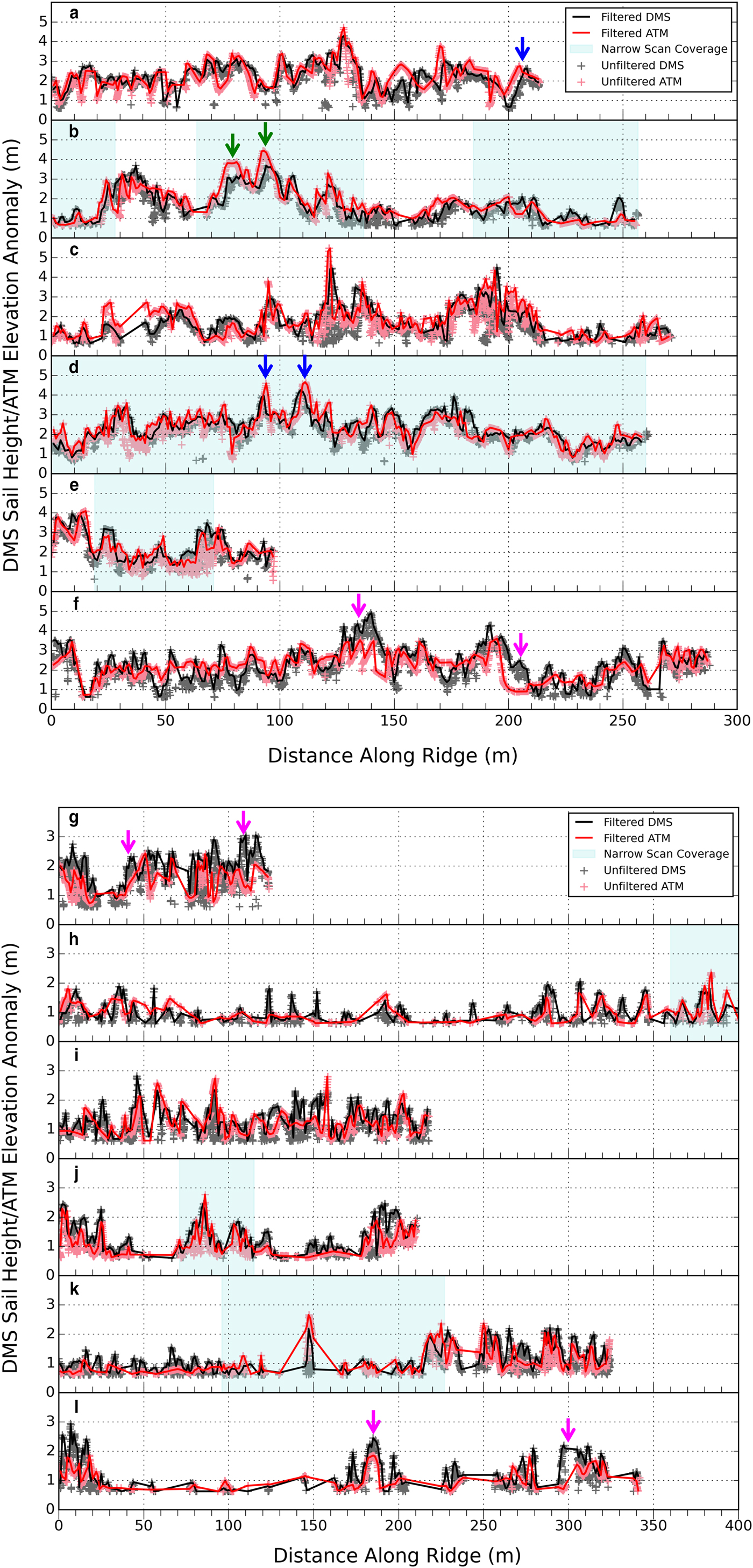
To mitigate differences in sampling density and directly examine differences, both H S and H A are resampled at 1 m resolution, so as to provide an equal number of measurements along the ridge crest. A ‘maximum value’ filter is applied such that the linear interpolation of H S and H A operates on the maximum height within each 1 m interval so as to identify measurements associated with ridge crests. For H S, the number of resampled data points at 1 m resolution is equivalent to the ridge length. H A may be resampled in three ways: using H A derived from the ATM wide- and narrow-scan measurements alone, or combining all available H A measurements. Resampled data are shown in Figures 5a and b as solid lines and make use of all available H S and H A measurements. There is consistency in the linear profiles for each ridge that demonstrates strong agreement between H S and H A (Figs 5a and b). High variability in sail heights along the crest of each pressure ridge, at very short length-scales of ~5 m, can also be observed. The blue, green and pink arrows in Figures 5a and b indicate instances where differences between H S and H A have occurred. Blue arrows delineate examples where the location of the maximum values of H S and H A are offset. This may be due to differences in the geolocation accuracy of the two instruments. Green arrows delineate examples where H S is lower than H A. This may be due to the obstruction of some shadows along the ridge crest by another intersecting feature on the sea-ice surface, such as a second pressure ridge segment or sastrugi. Pink arrows delineate some examples where H S is >H A. For these ridges (F, G and L) only ATM wide-scan data were available, and there were fewer total ATM measurements than interpolated 1 m samples. Thus, segments of the ridge crest may not have been sampled by the ATM due to its sparse sampling at the center of the ATM swath.
To determine the difference between H S and H A the ‘residual’ difference (H S−H A) is calculated, using the data resampled at 1 m. If both wide-scan and narrow-scan ATM data are available, separate residuals are calculated for each dataset for comparison with the DMS-derived sail heights. The Std dev. of the residuals is also calculated. Table 2 provides details of mean and Std dev. of the H S−H A residuals for all 12 ridges. Evaluating H S against the wide-scan ATM data, the residual mean and residual Std dev. range from −0.11 to 0.48 and 0.33 to 0.70 m, respectively (Table 2). Evaluating H S against the narrow-scan ATM data the residual mean and residual Std dev. range from −0.16 to 0.11 and 0.35 to 0.51 m, respectively (Table 2). The smaller residual means and standard deviations for the narrow-scan ATM data are expected and are due to the increased sampling density of the narrow-scan ATM along a segment of the ridge. This results in H A data that are more closely collocated with H S and hence provides a more direct comparison of H A with H S.
Scatterplots of sail height (H S) versus elevation anomaly (H A) for 12 pressure ridges (gray crosses). ATM data within one Std dev. (‘1σ edit’) of the mean residual (H S−H A) are highlighted for both the wide-scan (blue triangles) and narrow-scan (red stars) ATM data.
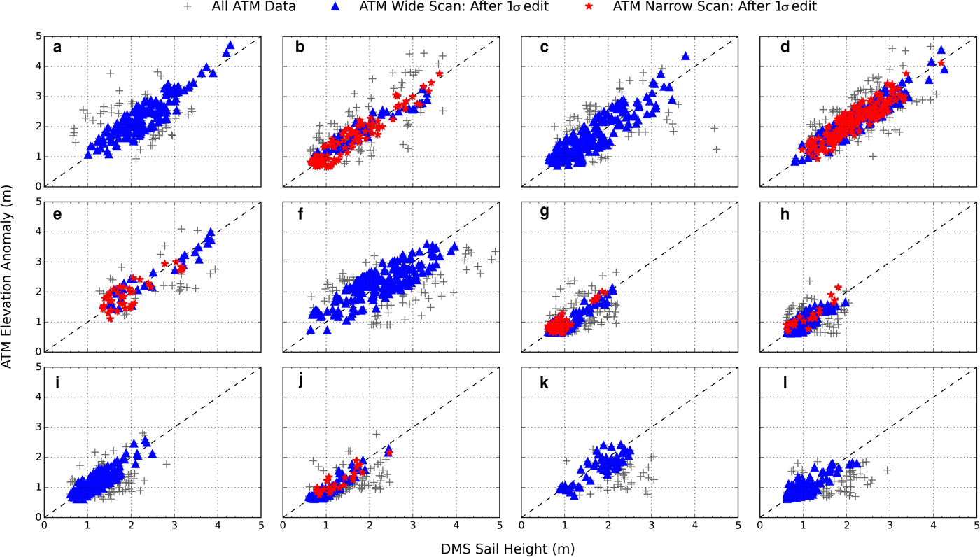
Residual (H S−H A) mean, residual Std dev. and correlation coefficient between H S and H A for 12 pressure ridge sails (A−L). Statistics refer to data shown in Figure 6

* ATM wide scan only.
† ATM wide and narrow scan.
To examine correlation, scatterplots of H S and H A are created, also using the H S and H A data resampled at 1 m (Fig. 6, grey crosses) for both the wide- and narrow-scan ATM measurements. Figure 6 suggests that H S and H A are strongly correlated, although, in the case of ridges A and B, H A appears slightly higher than H S, while for ridges F, I, J, K and L, H S appears slightly higher than H A. Using the residual mean and Std dev. results presented in Table 2, we draw attention to those data points that fall within one Std dev. of the residual mean (~68% of the data), for both the wide-scan and narrow-scan ATM data (blue and red triangles, respectively, Fig. 6). This editing acts to eliminate outliers arising from measurement noise, such as those discussed earlier. In all 12 cases, the data fall about the 1:1 line, indicating no apparent measurement bias between H S and H A. These data are used to compute the correlation coefficients between H S and H A, which range from 0.81 to 0.95 (Table 2). Both ATM wide-scan and narrow-scan data provide similarly strong correlation results.
SUMMARY
DMS imagery has been effectively utilized to determine pressure ridge sail heights on Arctic sea ice for the first time. We have demonstrated a new algorithm to identify and measure shadows cast by ridges and estimate sail height. DMS-derived sail height compares favorably with coincident ATM elevation anomalies. On average mean H S and H A agree to within 0.11 m and the distributions of H S and H A overlap. The correlation coefficient between H S and H A was 0.81 or greater for all 12 ridges, and scatter was closely distributed around the 1:1 line. No height biases were observed between ATM and DMS. These results provide confidence that the high-resolution DMS images, in conjunction with the new algorithm, produce reliable and accurate sail height measurements. This proof of concept study demonstrates the feasibility of using the DMS data to examine pressure ridge sail height. Moreover, the availability of DMS images over long transects of the polar oceans will provide an advancement in our ability to observe and interpret pressure ridge characteristics from an airborne platform. These initial results suggest that continued collection of DMS data over sea ice is warranted. The methods described here may be expanded to other airborne platforms, as well as applied to other high-resolution, visible imagery datasets.
Due to its rotating mirror and scan sampling geometry, the ATM lidar provides uneven sampling across the sea-ice surface. This results in a highly variable sample density and the number of available elevation anomaly measurements depends on the orientation of the pressure ridge with respect to the along-track direction of the ATM swath. Moreover, the swath widths of the wide-scan and narrow-scan lidars, at ~250 and ~45 m, respectively, limit the extent of the pressure ridge that may be observed. We have shown that the high-resolution DMS images provide a higher, and more even, sampling density along pressure ridges when compared with the ATM lidars. DMS sample density across the sea-ice surface is ~8.8 m−1, and the image dimensions result in a wider across-track observation of ~420 m (assuming a nominal flight altitude). We note that rotating the DMS camera by 90o would provide an increase in across-track coverage (up to ~650 m), although this would result in less overlap between consecutive images. On average, the DMS sampling of sail height outperforms the ATM by a factor of ~11 in the cases studied here. The average pixel resolution of the DMS imagery is 0.1 m and this provides an adequate sail height precision, representing ~6% of the signal, assuming an average sail height of 1.57 m.
Beyond demonstrating the efficacy of the DMS-based methodology for assessing sail height, the measurements from the 12 pressure ridges sampled in this study are intriguing. Both the along-track sail height profiles and the full sail-height distributions, indicate that the maximum sail height of new ridges formed in areas dominated by MYI ice (averaging 4.2 m) is approximately double those formed in the areas dominated by FYI (averaging 2.6 m). Ridges formed in areas of MYI also exhibited a wider range of sail heights. This is expected due to the older, thicker ice of a MYI floe, which generates thicker blocks of ice and in turn generates greater sail heights as ice blocks are piled on top of each other during the ridging process (Tucker and Govoni, Reference Tucker and Govoni1981).
These preliminary results warrant further investigation to examine if they apply more generally to the Arctic sea-ice cover. Having demonstrated that the method is viable, it may be applied to the full suite of DMS images. This task can be achieved by applying the methodology automatically to available DMS imagery. Although coincident ATM data (and alignment of ridges in the along-track direction) were required in this study to evaluate the DMS sail height results, neither is a requirement to apply the methodology to the full DMS collection. However, steps will be required to first discard any poor-quality DMS data gathered under cloudy or poor lighting conditions (Onana and others, Reference Onana2013). In a future study, we will analyze DMS data collected between 2010 and 2017 during OIB surveys of the western Arctic to develop a database of sail heights. We will examine the differences in the sail height distributions over FYI and MYI in more detail and assess the interannual variability in sail height and surface roughness during the OIB observation period.
SUPPLEMENTARY MATERIAL
The supplementary material for this article can be found at https://doi.org/10.1017/aog.2018.2
ACKNOWLEDGEMENTS
We thank the DMS and ATM instrument teams and the OIB science teams for collecting and processing the data utilized in this study. DMS and wide and narrow scan ATM data were acquired from the National Snow and Ice Data Center (NSIDC) at http://nsidc.org/data/iodms1b, http://nsidc.org/data/ilatm1b, and http://nsidc.org/data/ilnsa1b, respectively. This research was supported under NASA award NNX13AK36 G and by the NOAA Product Development, Readiness, and Application (PDRA)/Ocean Remote Sensing (ORS) program. We acknowledge the Editor, Marika Holland and two anonymous reviewers whose comments helped to improve the text. The views, opinions, and findings contained in this paper are those of the authors and should not be construed as an official NOAA or U.S. Government position, policy, or decision.


 Open access