


1. Introduction
Ice-sheet flow is driven by spatially and temporally varying accumulation, temperature and basal melt-rate fields. Unfortunately we usually have little knowledge about the detail of accumulation and the basal melt fields, especially over such vast areas as Antarctica. However, information about the flow field can be extracted from radio-echo sounding records, which image internal layers that result from variations in the dielectric properties of ice, due to variations in density, ionic concentration and crystal fabric (e.g. Reference Hempel, Thyssen, Gundestrup, Clausen and MillerHempel and others, 2000). An increasing body of evidence suggests that the variations in ice composition and morphology, which give rise to the reflections from these layers, were locked in at deposition, and that these layers are, in consequence, isochrones, i.e. deposited at the same time. Internal layers therefore contain significant information about the flow field. In addition, there is some less direct information regarding flowlines (e.g. accretion layers over subglacial lakes).
The connection between layer geometry and flow fields was originally pointed out by Reference WeertmanWeertman (1976) and recently has been discussed widely (Reference RaymondRaymond, 1983; Reference Nereson, Raymond, Waddington and JacobelNereson and others, 1998, Reference Nereson, Raymond, Jacobel and Waddington2000, Reference Nereson and Raymond2001; Reference Vaughan, Corr, Doake and WaddingtonVaughan and others, 1999; Reference Siegert, Hindmarsh and HamiltonSiegert and others, 2003; Reference Hindmarsh, Leysinger Vieli, Raymond and GudmundssonHindmarsh and others, 2006; Reference Parrenin, Hindmarsh and RémyParrenin and others, 2006). These studies show how spatial variations in the accumulation rate, basal melting, topography and basal sliding affect the layer geometry. In particular, Reference WeertmanWeertman (1976) showed how layers dip at the no-slip/slip transition, which we call the ‘Weertman effect’. Papers by Reference Fahnestock, Abdalati, Joughin, Brozena and GogineniFahnestock and others (2001) and Reference SiegertSiegert and others (2004a, Reference Siegertb) deal particularly with the influence of basal melting. As a general rule, spatial variation in accumulation rate induces the strongest patterns near the surface, while such variation in the basal conditions (melting rate or flow mode) induces the strongest changes near the bed. Similarly, horizontal variations in the viscosity of ice induce the strongest changes within the ice (e.g. the Raymond effect (Reference RaymondRaymond, 1983)). The changes propagate downstream and are consequently asymmetrical about the source of the disturbance.
Better knowledge of the layer architecture of disturbed isochrones therefore helps us to identify the source of the disturbance. Moreover, it is clear that there are at least two confounding effects: (1) radar lines are usually collected at arbitrary angles to the flow direction, and three-dimensional (3-D) effects consequently need to be understood; and (2) the various influences mentioned above often operate together, especially changes in basal melting and the flow mode (e.g. over subglacial lakes). Modelling and the visualization of results can assist us in this regard.
The modelling described in this paper is simple ‘stream-tube’ modelling. Upper and lower surface geometries are assumed, as are the accumulation rate and melting rate distributions and the flow mode. Flow is assumed to be parallel to the surface slope as in the shallow-ice approximation. These conditions are sufficient to define the balance fluxes, and the velocity distribution can be deduced and used to solve for the age of the ice. Stream-tube modelling allows rapid solutions to be obtained for layer age and other tracer fields (e.g. particle trajectories).
It can be objected that the distribution of sliding and melting have an effect on the surface geometry; however, at shorter wavelengths the transfer function from bed to surface is relatively weak (Reference GudmundssonGudmundsson, 2003; Reference Raymond and GudmundssonRaymond and Gudmundsson, 2005). A further, more specific objection is that the relationship between the bed, the accumulation rate and the basal properties should be computed ab initio, i.e. by prescription of the temperature field and internal viscosity and sliding coefficient. However, there is always a variation in internal viscosity or sliding coefficient which can produce the prescribed flow pattern. Rather than create it by the more complicated route of prescribing variations in viscosity and solving the Stokes equations (a highly computer-intensive calculation), we simply prescribe flow convergence using the slope of the ice and the balance flux formulation. Indeed, the balance flux formulation yields the viscosities as a by-product. Since this modelling is essentially in an exploratory phase, we ask what kinds of patterns are possible in principle, so the major added complication of prescribing viscosity distributions and solving the Stokes equations is not necessary at this point.
In this paper, we briefly outline the mathematical theory, consider two-dimensional (2-D) plane flows with changes in melting or basal traction, simulate near-plane flows in three dimensions and further simulate the isochrone patterns from radar lines that cross the flow direction, and then consider the interaction of surface perturbations.
2. Theory
Consider a coordinate system (r,z), where r = (x,y) with z pointing upwards. Extensive use is made of the steady continuity equation given by

where Q = (Qx ,Qy ) is the flux, a is the accumulation rate and m is the basal melt rate. This equation requires a boundary condition for Q where there is no flux out. In this paper, all such boundaries have condition Q = 0. Throughout this paper, ice thickness, accumulation and melt rate are constant over time. Equation (1) is used to compute the balance flux. Reference Budd and WarnerBudd and Warner (1996) and Reference HindmarshHindmarsh (1997) discuss the solution of this equation under the assumption that flow is parallel to the slope of the surface.
It is convenient to work in normalized coordinates (r, ζ, t) (where ζ is the ‘sigma’ coordinate and t is time), i.e.
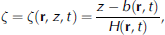
where b(r, t) is the height of the bed and H(r,t) is the thickness of the ice. Following Reference HindmarshHindmarsh (1999, Reference Hindmarsh, Straughan, Greve, Ehrentraut and Wang2001) the mapped ageing equation is



where X(r, ζ, t) is the age of the ice, Q(r, t) is the flux of ice in the region 0 ≤ ζ ≤ 1, and the partial flux q(r, ζ, t) is the flux of ice in the region 0 ≤ ζ ≤ ζ′. Note that, by definition, Q(r, t) = q(r, 1, t). The operators ∇H, ∇H. represent the horizontal gradient and horizontal divergence respectively along R surfaces of constant ζ. The partial flux q(r, ζ, t) = ζ 0 u(r, ζ 0, t) δζ 0 . Under the assumptions listed above,

where ū(r, t) is the vertically averaged velocity. The shape function for the horizontal velocity is


for uniform plug flow (S) and for isothermal internal deformation (ID) under the shallow-ice approximation with flow exponent n = 3. Under the same assumptions, the partial flux can be written in terms of the surface flux in the separable form q = Qω(ζ,r). For uniform plug flow and for uniform flow by internal deformation under the shallow-ice approximation, the flux shape function can be written as


(Reference LliboutryLliboutry, 1979; Reference RaymondRaymond, 1983; Reference HindmarshHindmarsh, 1999). More complicated forms arise when the rate factor A is a function of the height above the bed. Plug flow (which includes sliding) and internal deformation flow with a uniform rate factor are generally regarded as end-members of the range of possibilities, at least where the bed is flat. Generally non-isothermal flows lie in between these two end-members. To summarize, Equation (1) is used to compute the flux. The velocity distribution, in a form suitable for the age equation, can be deduced from the flux using Equations (4–6). These steps have eliminated the need to know the rate factor in the viscous relationship or sliding relationship. Given a geometry, the accumulation rate and a prescription of ω, all the information needed to solve the ageing equation (3) is present.
The model computations in this paper are as follows: modelling the isochrones over a flat bed with a region of basal melting and a region of sliding; using a slightly inclined surface which is (1) a planar surface and (2) a perturbed surface which consists of a channel in flow direction. In most cases in this paper, the velocity shape function prescribed describes plug flow (Equation (5a)). This corresponds either to sliding or to an internal deformation where most of the shear occurs in a very thin basal boundary layer owing to warming near the base (Fowler, 1992). This uniform shape function is used when we examine the effects of spatial variations in basal melting upon isochrone architecture; the point is that while of course one might expect changes in the velocity shape function when a region of high basal melting such as in a lake is reached, high sliding or highly concentrated basal shearing have very similar shape functions to that found in the shelf lying above a subglacial lake. The exception is a modelling suite where we wish to examine the effects of an abrupt change in the shape function on layer geometry. Here we define an internal area where sliding dominates, while outside this area we use the isothermal internal deformation shape function (Equation (5b)). Throughout this study the accumulation rate is uniformly 1 ma–1, and to prevent infinite ages at the base we prescribe a melt rate of 0.01 ma–1 throughout the domain (except where it has been specified to be higher).
Since we are considering isochrone geometry, we are not concerned with the actual age of the ice. The accumulation rate is essentially applied as a scale factor; for example, if the accumulation rate and melting rate were reduced by a factor of ten, the isochrone pattern would be exactly the same, but the age of the ice would be ten times greater (Reference Parrenin, Hindmarsh and RémyParrenin and others, 2006).
3. Effects of Melting: Plane and Quasi-Plane Flow
By prescribing an area with an increased melting rate of 1 ma–1 at the bed, we simulate a ‘hotspot’ and determine its effect on isochrones and the flowlines. This is carried out for plane flow and for a 3-D but essentially uniaxial flow. In this case, plug flow is prescribed throughout the domain.
3.1. Two-dimensional ice flow
In the 2-D case, we use two melting regions each extending 50 km in the x direction. This configuration is chosen to show the effect of horizontal velocity, as the downstream melt zone experiences a greater flux. Figure 1a shows a transect along a flow plane with the two melting regions of identical melt rates (1ma–1). The isochrones are deflected over both hotspots and dip towards the bedrock (Fig. 1, solid lines). The largest depression is at the downstream margin of the melting spot. Ice is lost along the full area of melt, and consequently the greatest thickness of ice (number of isochrones) is lost at the lower end of the area. This is also shown in the flowlines in Figure 1 (dotted lines), where at the downstream margin of the melt area a greater amount of younger ice is melted away than at the upstream margin. The depression of the isochrone decreases towards the surface. This description applies to both melting spots, but over the downstream spot the isochrones are less deformed. This is due to the difference in horizontal velocity; the dip in flowlines is related to the ratio of downward velocity (melting) to horizontal velocity, and this has consequent effects on the flowline geometry.
Effect of increased basal melting on isochrones (solid lines) and on flowlines (dotted lines) in plane flow. The two areas of increased basal melting, each of 50 km length, are indicated by a black bar. Isochrone ages are in kyr and shown in contours filled in greyscale.

Some distance downstream of the melt spot, the isochrones revert to their initial height within the ice. This occurs where ice particles have never been affected by the melting area. Flow over a subglacial bump has a similar effect (Reference Parrenin, Hindmarsh and RémyParrenin and others, 2006). Reference SiegertSiegert and others (2004a) also model plane transects over regions of enhanced melting and compute comparable patterns.
3.2. Three-dimensional ice flow
We now consider 3-D quasi-plane flow. Only one area of high melting is specified. With the 3-D model we can look at transects at any angle to the flow direction, giving us the opportunity to investigate how isochrone disturbances by melting or sliding are pictured in profiles not parallel to the flow. This is useful when interpreting isochrones in radar profiles.
The melting area is a 50 km by 50 km square. The positions of several transects at different angles in relation to the melting area are shown in Figure 2. The transects deviate from the flow direction by 90˚ or 45˚ from their origin. Figure 3a–c show the transect along a profile transverse to the main flow. Here the isochrones show a depression over the melting area, which can be seen to be increasing downstream in successive transects (Fig. 3a–c). Isochrones to the right and the left flanks of the hotspot are undisturbed, as a consequence of the specification of a planar surface which does not permit lateral inflow as might happen more generally. From an observational viewpoint, the isochrones along the transverse transect have more similarities with the Weertman effect in Figure 4 than with the sliding effect along the flow in Figure 1a. The transects at 45˚ to the flow direction (Fig. 3d–f) show a pattern similar to the along-flow pattern (Fig. 1) for Figure 3d and e, as these intersect the flank of the melting zone. Where the line intersects the downstream edge (Fig. 3f), a more complex pattern is seen, because the isochrones downstream of the melting area have not yet reverted to the previous height. Without knowledge of the flow-field and basal conditions, such an isochrone pattern could easily be misinterpreted.
Aerial view of a section of the modelling domain showing the absolute flux (m2 s–1) in contours (filled in greyscale) and arrows, visualizing the flow direction, obtained for (a) a planar surface and (b) a surface with a central along-flow depression (Equation (8)). Superimposed thick dark grey lines outline the areas of melting and sliding, respectively, and the different transects (thick black) shown as: (a, d, g) dashed lines, (b, e, h) dashed-dotted lines and (c, f, i) solid lines.

Melting effect with plane flow: isochrones along transects cutting the flowlines at 90˚ (a–c) and 45˚ (d–f). The positions of transects (a–f) are shown in Figure 2a. The isochrone contours filled in greyscale are in kyr. The area of increased basal melting is indicated by a black bar. Note that for transects (d–f) the melting zones are of varying length.

Effect of areas with basal sliding (Weertman effect) on isochrones (solid lines) and on flowlines (dotted lines) in plane flow. The two regions of basal sliding, each of 50 km length, are indicated by a black bar (no-slip condition above white regions). Isochrone ages are in kyr and shown in contours filled in greyscale.

4. Effects of Changes in the Flow mode: Plane Flow and Quasi-Plane Flow
Changes in the sliding mode were first discussed by Reference WeertmanWeertman (1976), and some direct computations of isochrone geometry near flow-mode transitions using the full system of stress equations have been presented by Reference Hindmarsh, Leysinger Vieli, Raymond and GudmundssonHindmarsh and others (2006; see, e.g., fig. 7 therein). The influence of horizontal stress gradients is to smooth, but not eliminate, the features associated with the flow-mode transition, in particular the downward and upward steps. The smoothing occurs over a zone with horizontal extent corresponding to a few ice thicknesses. This distance is small compared with those we are considering here, so it is appropriate to model the change in shape function as a jump.
In these studies, the bulk of the domain flow is by internal deformation. Smaller regions are prescribed where flow is by sliding, and plug flow thereby induced. In this way we simulate the effects of either a small ice stream or a lake with a small background melting of 0.01 ma–1. This is carried out for plane flow and for a 3-D but essentially uniaxial flow. In fact, in the calculations we have smoothed the transition from complete internal deformation to complete sliding, as the finite-difference algorithm was unable to represent the changes adequately. The smoothing is carried out using a weighting formula

where C is the x coordinate of the centre point of the sliding region, L is its extent in the x direction and where ωS is given by Equation (6a) and ω ID by Equation (6b). We set α = 20, which represents a sharp step, while allowing the numerical results to converge to sufficient accuracy as the grid was refined.
4.1. Two-dimensional ice flow
Figure 4 shows the isochrones (solid lines) and the flowlines (dotted lines) for a plane-flow transect with two sliding areas, each of 50 km length. At the upstream and downstream margin we observe the ‘Weertman effect’ (Reference WeertmanWeertman, 1976), where the isochrones sink towards the bed when there is a change from no-slip to slip and vice versa (Fig. 4, solid lines). This effect is also manifested in the flowlines (Fig. 4, dotted lines).
If there is an abrupt jump in the flow mode, there is a corresponding abrupt step in the isochrone elevation. By a further coordinate transform into a ω coordinate, F. Parrenin and R. Hindmarsh (unpublished information) show that the step is proportional to the change in the flux shape function ω (see Equations (6)) in the transition from internal deformation to sliding. The maximum step in isochrone elevation at the flow-mode transition, considered as a function of elevation above the bed, occurs where the horizontal velocity shape functions (5) are equal, because this corresponds to the elevation where the maximum jump in partial flux q occurs (since v = ω
'). Thus, by equating (5a) and (5b) and solving for the elevation of maximum change in isochrone elevation ζ
MC, which is found to be  . For ice with n = 3, this occurs at about ζ 0:331. This formula is also derived in F. Parrenin and R. Hindmarsh (unpublished information), who explicitly consider the evolution of isochrone slope as a consequence of changes in the flow mode.
The near-basal isochrones above the sliding area slope towards the bedrock in the downstream direction. The tilt of the slope is reversed in isochrones further away from the bed, and the maximum tilt in slope is found in the middle of the ice mass. This can be explained as follows. Consider a particle whose flow takes it exactly through the elevation of maximum downward step ζ MC at the ID–sliding transition. Call its trajectory the TIEMC (trajectory intersecting elevation of maximum change). Trajectories above the TIEMC will have experienced a smaller step downwards. Such particles will consequently descend less in a given time, and isochrones will therefore tilt upwards in the direction of flow. In a similar way, trajectories below the TIEMC will cause isochrones to tilt downwards in the direction of flow. As one moves downstream, the elevation of the TIEMC decreases (at least until the reverse flow transition is met), so the elevation of the transition from tilting up to tilting down decreases.
At the downstream margin of the sliding zone, the upper, upwards-tilting isochrones rise, overriding the slower-moving ice at the base. They can rise to be higher than their elevation upstream of the sliding zone. This is because the reverse transition has occurred at a lower elevation which corresponds to a greater step in elevation. Eventually the isochrones revert to their initial state as described above in section 3.1 (Reference Parrenin, Hindmarsh and RémyParrenin and others, 2006).
This description applies to both sliding spots, but, in contrast to the basal melting case, the pattern of isochrones is very similar for both.
4.2. Three-dimensional ice flow
Again the 3-D quasi-plane-flow case is quite similar to the 2-D case. An issue is the transition from sliding to internal deformation only, which is very abrupt. Figure 5 shows the isochrones along those transects. Figure 5a–c show the transect along a transverse profile. On those transects the isochrones show a depression over the sliding zone which increases downstream (Fig. 5a and b); however, the transect along the downstream margin also features isochrones nearer to the surface with a bump (Fig. 5c). Where transects are oriented at 45˚ to the main flow (Fig. 5d–f) isochrones show a pattern similar to those for the plane-flow case (Fig. 4), except in the case where the transect runs through ice downstream of the sliding area that is still affected by the disturbance, such as shown in Figure 5f. Here the isochrones show a trough followed downstream by a bump. Again, when viewed on its own, without knowing the flow-field context, such a pronounced isochrone pattern could lead to misinterpretations of the cause for this pattern.
Sliding effect with plane flow: isochrones along transects cutting the flowlines at 90˚ (a–c) and 45˚ (d–f). The positions of transects (a–f) are shown in Figure 2a. The isochrone contours filled in greyscale are in kyr. The area of basal sliding is indicated by a black bar. Note that for transects (d–f) the sliding zones are of varying length.

5. Additional Effect of Flow Divergence
We now examine the effect of diverting flow into a channel by small changes in the surface topography. This creates lateral gradients in the downstream velocity. Again we consider isochrones calculated with the 3-D model along transects traversing a region of either melting or sliding. Flow diversion on its own without further perturbation produces no effects on the isochrone architecture.
The channel is formed by subtracting a cosine function from the surface s,

with an amplitude B = 1.6 m and a wavelength λ = 200 km located transverse to the flow (see Fig. 2b). Results are shown in Figure 6: the top row (Fig. 6a–c) shows transects parallel to the main flow direction for the case of variable melting; the second row (Fig. 6d–f) shows transects transverse to the flow direction for the same case; while the third row (Fig. 6g–i) shows flow-transverse transects for the case of changes in the flow mode. The changes in the basal forcing are specified similarly to the previous cases.
Basal melting (a–f) and basal sliding (g–i) effect with a channel: isochrones along transects parallel to main flow (a–c) and cutting the centre flowline at 90˚ (d–i). The amplitude of the surface perturbation cosine is 1.6 m. The positions of transects (a–i) are shown in Figure 2b. The isochrone contours filled in greyscale are in kyr. The area of basal melting/basal sliding is indicated by a black bar.

The first thing to notice in the top row of Figure 6 is that small changes in lateral position, corresponding to rather larger changes in the downstream velocity, have marked effects on the isochrone geometry, in particular the length scales over which the isochrones change in response to changes in the basal forcing. Along the centre line (Fig. 6a) the flow accelerates downstream, and the slope of the isochrone after the zone of melting is particularly low, at least compared with Figure 6b, where velocities are less.
These effects result in some surprising features in the transverse sections (Fig. 6d–f). While the overall response is a dip in the isochrones, as we anticipate from previous examples, the more elongated response in faster-flowing regions results in the dip being less marked and a bump in the isochrone when viewed in the transverse section. Immediately adjacent to the flanks, we see a relatively gentle dip of the isochrones rather than the abrupt step seen in the previous examples. This is due to the lateral inflow, which advects the isochrone pattern in from the side. Convergence flow over melting regions could contribute to the radar-detected internal folds in ice streams (e.g. Reference Ng and ConwayNg and Conway, 2004).
When changes in flow mode are considered, an even more complex set of phenomena emerges. Figure 6g–i show a double bump, or three troughs. The central trough can be explained as above by the increase in velocity. At the change in the flow mode, there is a downward step in the isochrones. The upper layers slope upwards, but the slope depends upon the velocity, and is less in magnitude for faster ice (Fig. 4), hence the trough. Towards the flanks we again see the lateral inward flow producing a downward step in the isochrones. Since the slope of the isochrones is reversed near the base, one might expect to see the patterns of bumps and troughs reversed here, but it is perhaps too subtle to discern.
6. Conclusions
Modelling reveals that the interpretation of isochrones without prior knowledge of basal condition is a very difficult task. It is made much harder where data are connected obliquely to the ice-flow direction.
-
1. When viewed in sections parallel to the flow direction, 3-D flows incorporating either changes in the flow mode (sliding, no-sliding) or increased melting appear similar to plane flows. Isochrones are markedly asymmetric in the flow direction, and this effect dominates observations.
-
2. An increase in melting and the transition from internal deformation to sliding both produce dips in the isochrones, but these are of somewhat different character. The immediate effect is much more marked for the change in sliding (i.e. the Weertman effect), but the subsequent development of isochrones shows different patterns: in the case of melting, they continue to dip, while with changes in flow mode they slope upwards in the upper part of the ice, downwards in the lower part of the ice immediately after the flow-mode transition and then upwards again further downstream.
-
3. Bumps and troughs are found in transects perpendicular to the flow in the presence of lateral gradients in the downstream velocity when there are also changes in melting or flow mode, and may be related to folds in ice streams (e.g. Reference Ng and ConwayNg and Conway, 2004). The shape of the bumps and troughs depends on the lateral gradient of the velocities and can be explained by more elongated responses to changes in flow conditions for faster-moving ice. In addition, lateral inflow changes the patterns of isochrones near the flanks of hotspots or high-sliding zones.
-
4. Seemingly anomalous flow patterns can be found when a transect runs transversely through ice downstream of a disturbance which is still affected by the disturbance. For example, we have shown cases where isochrones are raised downstream of a sliding zone into a considerable bump. Without understanding of the flow-field context these patterns could be misinterpreted, which highlights the importance of modelling.
-
5. Flow convergence, melting and changes in flow mode, when coupled together, affect isochrones over the whole depth of the ice sheet. Changes near the top cannot be solely attributed to spatial variation in the accumulation rate.
Acknowledgements
We thank the referees for detailed reviews and comments which considerably improved the paper. Funding for work leading to this paper was provided by UK Natural Environment Research Council grant No. NER/A/S/2001/01011.



