
I. INTRODUCTION
Although a large number of studies have been made on denoising, most of them are focused on utilizing correlation between pixels. In regression filters, a convolution kernel was determined based on the spatial distance between pixels [Reference Wand and Jones1,Reference Gonzalez and Woods2]. Those were extended to bilateral filters introducing the photometric distance [Reference Zhang and Gunturk3,Reference Honghong, Rao and Dianat4]. Recently, interests in non-local mean (NLM) filters have been growing [Reference Buades, Coll and Morel5–Reference Milanfar10]. This class of filters replaces pixel-wise calculation of the distance with patch-wise one. Reports on the NLM filter have been actively studied, such as improvement of denoising performance [Reference Liu, Zhong and Jiao11–Reference Ghosh, Mandal and Chaudhury13], processing speed [Reference Chan, Zickler and Lu14–Reference Huang16], combination of NLM filter, and another method [Reference Mohan and Sheeba17,Reference Kim, Park, Han and Hanseok18].
Later on, NLM filters have been developed to be adaptive to the local statistics of an image with the introduction of the prior knowledge in a Bayesian framework [Reference Lebrun, Buades and Morel19–Reference Aguerrebere, Almansa, Delon, Gousseau and Muse25]. Lebrun et al. proposed the non-local Bayes algorithm in which the patch is modeled as a Gaussian distribution and its parameters are computed from a local neighborhood [Reference Lebrun, Buades and Morel19]. This kind of technique was referred to as the hierarchical Bayesian modeling [Reference Gelman, Carlin, Stern and Rubin20] and applied to the image restoration [Reference Molina21,Reference Molina, Katsaggelos and Mateos22], the image un-mixing problem [Reference Dobigeon, Tourneret and Chang23] and the image de-convolution [Reference Orieux, Giovannelli and Rodet24]. Recently, it was extended to be stable against the missimg problem [Reference Aguerrebere, Almansa, Delon, Gousseau and Muse25]. All of them share a common Bayesian framework based on the prior knowledge on parameters of the Gaussian distribution for each local patch.
Unlike those Bayesian approaches, we utilize the prior knowledge, not on the local patch in NLM but, on the noise bias (NB) which is newly introduced in this paper. Most of the literatures usually assume the noise to be i.i.d. additive white noise. Especially, the zero-mean assumption has been widely imposed on the filter design [Reference Dabov, Foi, Katkovnik and Egiazarian9,Reference Milanfar10]. However, in tone mapping (TM) processing [Reference Reinhard, Stark, Shirley and Ferwerda26–Reference Koz and Dufaux28], such as brightness correction, contrast adjustment for dark images, or RAW images, the output noise has a non-zero average (= NB). This NB is due to the non-linearity of TM such as the power function, the logarithmic function, and the Hill function, etc. However, little attention has been given to NB.
This paper tries to recover the ideal output image from the observed output image by compensating NB. The NB is a different notion from the ensemble average of the noise over “all” pixels. In this paper, pixels in the noisy image are classified into several subsets according to the observed pixel value, and compensates the pixel value in each subset with a preliminarily determined compensation value. This procedure is the NB compensation (NBC). NB in this paper is the mean of the noise in the subset corresponding to the observation pixel value and it is compensated. A primitive idea was reported in [Reference Iwahashi and Kiya29]. Extending the idea, a method of determining the compensation value from all pixel values in an input image based on the Bayesian inference theory was reported without enough experimental results [Reference Iwahashi, Hamzah, Yoshida and Hitoshi30]. In addition, it is assumed that all histogram information of an input image is included in the overhead information.
In this paper, we propose a new method based on compensation value calculated from reduced information of the histogram of an input image and the noise before TM. In the proposed method, it is assumed that the histogram of the pixel values in an input image is included in the overhead information which is reduced much more than [Reference Iwahashi, Hamzah, Yoshida and Hitoshi30].
This paper is organized as follows. Section II describes the problems dealt with in this paper. Section III describes the proposed method. Section IV shows experimental results using night scene images and confirms effectiveness of the proposed method. Finally, the paper is concluded in Section V.
II. PROBLEM SETTING
Figure 1 illustrates a situation this paper assumes. An image is assumed to have additive noise. The noisy image is tone mapped (brightness corrected). As a result, NB becomes non-zero value. This paper compensates the NB of the noisy image after TM. This paper regards a night scene image and a tone mapped noisy image as an input image and an observed output image, respectively, and assumes noise as Gaussian noise. Section A describes effect of TM on noise, and Section B describes NB after TM.
A situation this paper assumes.

A) Effect of tone mapping on noise
In this paper, we consider the case where a noisy image is tone mapped. Figure 2 illustrates examples. The input image signal is expressed as
 $$x_0({\bf{n}}) = x_0(n_1, n_2), \quad x_0 \in [0, X_{MAX}] \subseteq {\open Z},$$
where  $x_0({\bf{n}})$ denotes a pixel at location ${\bf{n}}=[n_1,\, n_2]$ and $X_{MAX}=255$. We shall omit the coordinate ( ${\bf{n}}$) when we are looking at a particular pixel and the position is not important. A pixel value $x_0$ is tone mapped with a function f as
 $$y_0 = R[ f(x_0) ], \quad y_0 \in [0, Y_{MAX}] \subseteq {\open Z},$$
where a pixel value  $y_0$ is the ideal tone mapped value and $Y_{MAX}=255$. $R[\ ]$ denotes rounding to the nearest integer and is defined as
 $$R[x] = \lfloor x + 2^{-1} \rfloor.$$
Example images before and after TM; (a) and (d) are images before TM; (b) and (e) are images after TM with  $\gamma =3$. (a) Input image, (b) ideal output image, (c) input noise $(\sigma = 8)$, (d) noisy image, (e) observed output image, (f) observed output noise.

As the simplest example, γ correction is used as the TM function in this paper. TM function f is formulated as
 $$f(x) = \left\{\matrix{0 \hfill & {\rm for} \hfill & x \lt 0 \hfill \cr Y_{MAX} \cdot (X_{MAX}^{-1} \cdot x)^{1/\gamma} \hfill & {\rm for} \hfill & x \in [0, X_{MAX}] \cr Y_{MAX} \hfill & {\rm for} \hfill & x \gt X_{MAX},\hfill}\right.$$
 where γ is a parameter. For a given noise  $\varepsilon _1({\bf{n}})$ is expressed as
 $$\varepsilon_1({\bf{n}}) = \varepsilon_1(n_1, n_2),$$
a pixel value  $x_1$ in the noisy image is expressed as
 $$x_1 = x_0 + \varepsilon_1,$$
where  $x_1$ is clipped to the range of $[0,\, X_{MAX}]$. In Fig. 2, the probability mass function (PMF) of the noise $\varepsilon _1$ on $x_0$ is given as the Gaussian function
 $$P(\varepsilon_1 | x_0) = {1\over \sqrt{2\pi}\sigma} \, {exp} \left( - {\varepsilon_1^2\over 2 \sigma^2} \right),$$
where  $\sigma ^2$ denotes the variance and the mean of the noise is zero value. A pixel value $y_1$ which is a tone mapped value of $x_1$ is expressed as
 $$\eqalign{y_1 & = f(x_1) \quad \cr & = f(x_0 + \varepsilon_1) \quad \cr & = y_0 + \delta_1,}$$
where  $\delta _1$ denotes an observed output noise. Figures 3(a) and 3(b) illustrate the flow of TM for an input image and a noisy image, respectively.
(a) Flow of TM for an input image.  $y_0$ is the ideal tone mapped pixel value. (b) Flow of TM for a noisy image. The mean of output noise $\delta _1$ included in an image after TM hasa non-zero value. (c) Flow of NBC.

B) Noise bias after tone mapping
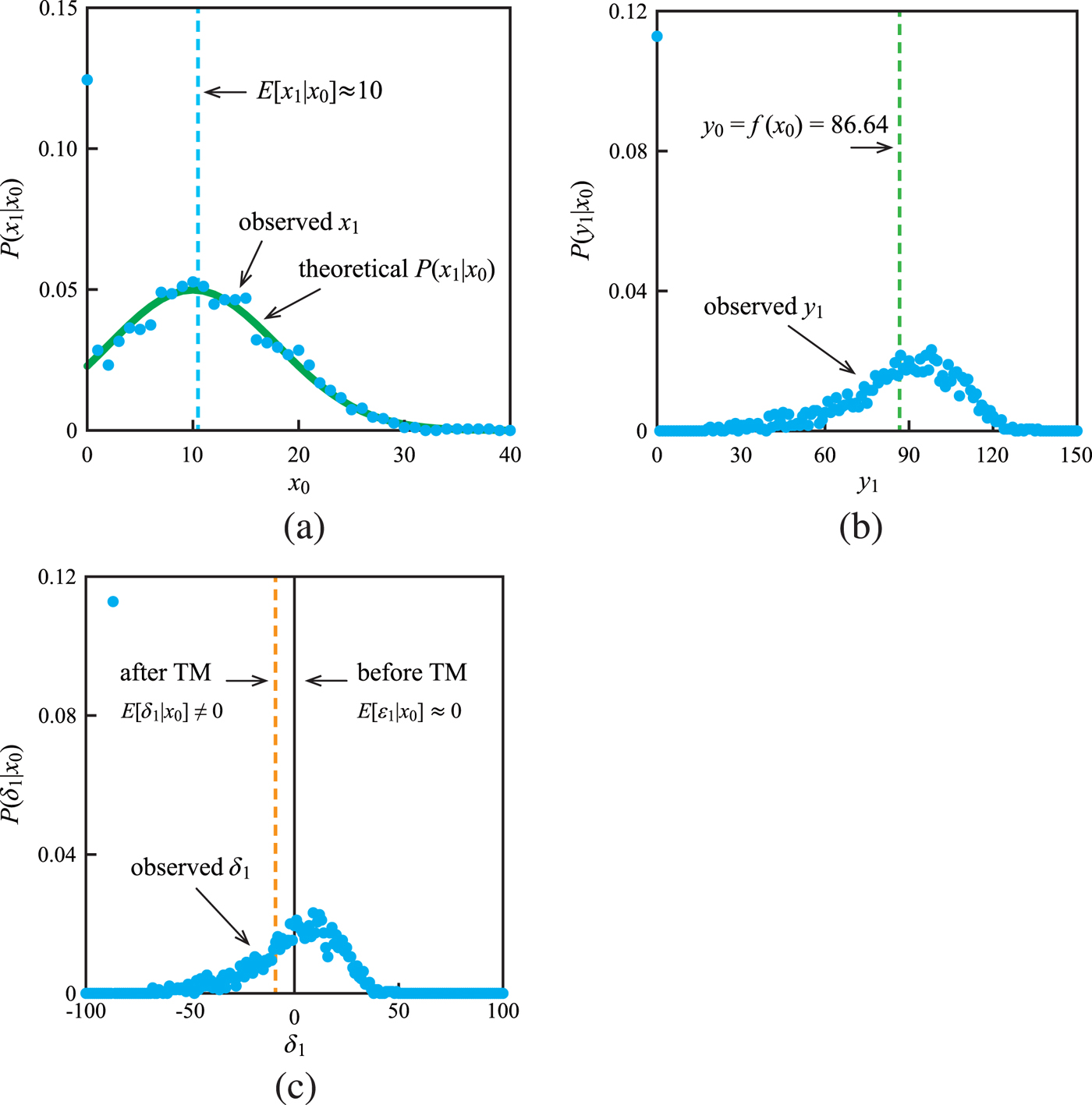
In an image processing such as TM, an output noise which is included in an image after TM hasa non-zero mean. We investigate the PMF of pixel values before and after TM. Figure 4(a) illustrates the conditional-PMF  $P(x_1|x_0)$ at $x_0=10$. It seems that the observed $P(x_1|x_0)$ (= blue dots) and the theoretical $P(x_1|x_0)$ (= green curve) are almost the same. The conditional mean $E[x_1|x_0]$ approximates 10 ( ${=}x_0$). $P(x_1|x_0)$ is formulated as
 $$P(x_1|x_0) =\left\{\matrix{\sum\nolimits_{t=-\infty}^{0} g(t|x_0) \hfill & {\rm for}\quad x_1 = 0 \hfill \cr g(x_1|x_0) \hfill & {\rm for} \quad x_1 \in (0, X_{MAX})\hfill \cr \sum\nolimits_{t=X_{MAX}}^{\infty} g(t|x_0) \hfill & {\rm for} \quad x_1 = X_{MAX}\hfill \cr 0 \hfill & {otherwise},\hfill}\right.$$
where
 $$g(x_1|x_0) = {1\over \sqrt{2\pi} \sigma} \, exp \left( - {(x_1-x_0)^2\over 2 \sigma^2} \right).$$
Figures 4(b) and 4(c) illustrate the conditional-PMF  $P(y_1|x_0)$ and $P(\delta _1|x_0)$, respectively. In Fig. 4(b), $P(y_1|x_0)$ is asymmetric with respect to the ideal tone mapped value $y_0$, and a bias is generated. In Fig. 4(c), although the mean of the noise before TM isa zero value, the mean of an output noise $\delta _1$ isa non-zero value (= NB). The next section introduces a new method to compensate NB. This is the fact we are focusing on in this paper.
(a)  $P(x_1|x_0=10)$. $x_0$ and $x_1$ are pixel values in an input image and a noisy image, respectively. The mean of an input noise $\varepsilon _1$ is a zero value. (b) $P(y_1|x_0=10)$. $y_1$ is pixel values in an image after TM. (c) $P(\delta _1|x_0=10)$. $\delta _1$ is noise in an image after TM. The mean of an output noise $\delta _1$ isa non-zero value.
III. PROPOSED METHOD
In Section II, it was shown that the mean of output noise after TM has NB. This paper tries to recover the ideal output image from the observed output image by compensating NB. In this section, we propose NBC which is a new method based on compensation value calculated from prior knowledge.
A) NB compensation
In order to recover the ideal output image from the observed image, a calculated value of NB (compensation value) is subtracted from an observed pixel value. NBC is defined as
 $$\eqalign{y_2 &= y_1 - h(y_1) \cr &= y_0 + \delta_2,}$$
where  $y_2$ is a pixel value after NBC, $h(y_1)$ is a compensation function giving the compensation value for the observed pixel value $y_1$ and $\delta _2$ denotes the error with respect to the ideal tone mapped value. Figure 3(c) illustrates the flow of NBC.
Note that unlike the Bayesian MAP estimation which maximizes the posterior probability density function [Reference Liu, Freeman, Szeliski and Kang31–Reference Sadreazami, Ahmad and Swamy34], our method calculates the compensation value from a subset according to the observed pixel value as indicated in equation (11).
B) Subset according to the observed pixel value
Figure 5(a) illustrates the conditional-PMF  $P(x_0|y_1)$ at $y_1=100$. Let N be the set of all pixels in an image and ${M}_{y_1}$ the set of pixels that derive the observed pixel value $y_1$. Note that ${M}_{y_1}$ is a subset of N;
 $$\left\{\eqalign{& {N} = \left\{{\bf{n}} \in {image} \right\}, \cr & {M}_{\eta} = \left\{{\bf{m}} | y_1({\bf{m}}) = \eta \right\} \subseteq {N}.} \right.$$
For a pixel value in Fig. 5(a) expressed as  $x_0({\bf{m}})$, Fig. 5(b) illustrates the conditional-PMF of an output noise.
(a)  $P(x_0|y_1=100)$. The pixel value $x_0$ is the subset according to the observed pixel value $y_1=100$. (b) $P(\delta _1|y_1=100)$. (c) Relationship between $\delta _1$ and $x_0$. The mapping from $\delta _1$ to $x_0$ is a bijective.

C) Compensation function
In this paper, the compensation value for the observed pixel value  $y_1$ is defined as the conditional mean of the observed output noise $\delta _1({\bf{m}})$. Therefore, the compensation function is defined as
 $$\eqalign{& h(y_1)=E[\delta_1|y_1] \cr & \quad \quad = {1\over |{M}_{y_1}| } \sum_{{\bf{m}} \in {M}_{y_1}} \delta_1({\bf{m}}).}$$
Equation (13) is equivalently expressed as
 $$\eqalign{h(y_1) &= \sum_{ {\bf{m}} \in {M}_{y_1} } P \left( \delta_1({\bf{m}}) \right) \cdot \delta_1({\bf{m}}) \cr & = \sum_{ {\bf{m}} \in {M}_{y_1} } P \left( \delta_1({\bf{m}}) \right) \cdot \left( y_1 - y_0\right) \cr & = \sum_{ {\bf{m}} \in {M}_{y_1} } P \left( \delta_1({\bf{m}}) | y_1 \right) \cdot \left( y_1 - y_0\right)}$$
Note that  $P ( \delta _1({\bf{q}}) | y_1 ) = 0$ where ${\bf{q}} \in \overline {{M}_{y_1}} \subseteq {\rm N}$. Therefore, equation (14) is equivalently expressed as
 $$h(y_1) = \sum_{{\bf{n}} \in {N}} P \left( \delta_1({\bf{n}}) | y_1 \right) \cdot \left( y_1 - y_0\right).$$
Here, the mapping from  $\delta _1$ to $x_0$ is a bijective. Because, using equation (8), the observed output noise $\delta _1({\bf{m}})$ is expressed as
 $$\delta_1({\bf{m}}) = y_1 - f( x_0({\bf{m}}) ),$$
equivalently expressed as
 $$x_0({\bf{m}}) = f^{-1}( y_1 - \delta_1({\bf{m}}) ).$$
Figure 5(c) illustrates the relationship between  $\delta _1({\bf{m}})$ and $x_0({\bf{m}})$. Since the relationship between $\delta _1({\bf{m}})$ and $x_0({\bf{m}})$ is the bijective, the following equations hold.
 $$\eqalign{P \left( \delta_1({\bf{m}}) \right) &= P \left( x_0({\bf{m}}) \right)\quad \cr P \left( \delta_1({\bf{n}}) | y_1 \right) &= P \left( x_0({\bf{n}}) | y_1 \right).}$$
Substituting equation (18) into equation (15),
 $$\eqalign{h(y_1) &= \sum_{ {\bf{n}} \in {N} } P \left( x_0({\bf{n}}) | {y_1} \right) \cdot \left( y_1 - y_0\right) \cr \quad &= \sum_{ x_0 } P \left( x_0 | y_1 \right) \cdot \left( y_1 - y_0\right).}$$
According to the Bayes' theorem and the addition theorem,
 $$P(x_0|y_1) = {P(x_0,y_1) \over P(y_1)},$$
and
 $$P(y_1)=\sum_{x_0} P(x_0,y_1). $$
hold, respectively. Substituting equations (20) and (21) into equation (19),
 $$\eqalign{& h(y_1) = \sum_{ x_0 } { P(x_0,y_1) \over P(y_1) } \cdot \left\{ y_1 - f(x_0) \right\} \cr & \quad \quad = {\sum_{ x_0 } P(x_0,y_1) \cdot \left\{y_1 - f(x_0) \right\}\over { P(y_1) }} \cr & \quad \quad= { \sum_{ x_0 } P(x_0,y_1) \cdot \left\{y_1 - f(x_0) \right\}\over { \sum_{x_0} P(x_0,y_1)}}.}$$
The joint-PMF  $P(x_0,\,y_1)$ is the “prior knowledge” which can be obtained using all pixel values $x_0$ in an image. Figure 6 illustrates the TM function and the prior knowledge.
(a) TM function ( $\gamma =3$). (b) $P(x_0,\,y_1)$. (c) $P(x_0,\,x_1)$. (d) $\hat {P}(x_0,\,y_1)$. $P(x_0,\,y_1)$ and $\hat {P}(x_0,\,y_1)$ is the prior knowledge. Note that the log-scaled joint-PMF is illustrated.

Note that it is assumed that all pixel values in an input image are included in the overhead information. If the histogram of pixel values in an input image is included in the overhead information instead of all pixel values, it becomes possible that the overhead is reduced. In the next section, we introduce the modeling of prior knowledge  $P(x_0,\,y_1)$ from the histogram of pixel values in an input image and that of the noise before TM.
D) Modeling of PMF
In this paper, we propose a method of determining the compensation value from the histogram of pixel values in an image and that of the noise before TM based on the Bayesian inference theory. Let modeled prior knowledge be  $\hat {P}(x_0,\,y_1)$. In the sequel, we derive a reasonable model $\hat {P}(x_0,\,y_1)$ assuming only the knowledge of $P(x_0)$ (= the histogram of pixel values in an input image before TM) and $g(x_1)$ (= the histogram of the noise before TM) as the overhead information. The compensation function using $\hat {P}(x_0,\,y_1)$ is expressed as
 $$\hat{h}(y_1) = { \sum_{ x_0 } \hat{P}(x_0,y_1) \cdot \left\{ y_1 - f(x_0) \right\} \over \sum_{ x_0 } \hat{P}(x_0,y_1) }.$$
 The prior knowledge  $P(x_0,\,y_1)$ is obtained by mapping the joint-PMF $P(x_0,\,x_1)$ shown in Fig. 6(c) according to the gradient of the TM function. According to the Bayes' theorem,
 $$P(x_0,x_1) = P(x_1|x_0) P(x_0),$$
holds. In this modeled case, it is assumed that the prior probability  $P(x_0)$ is included in the overhead information. From (9), the posterior probability $P(x_1|x_0)$ is modeled as
 $$\hat{P}(x_1|x_0) = \left\{\matrix{{\sum\nolimits_{t=x_0-3\sigma}^{0}} g(t|x_0) \hfill & {\rm for} \quad x_1=0 \hfill \cr {}\hfill &\quad\quad \wedge x_0-3\sigma \leq 0 \hfill \cr g(x_1|x_0) \hfill & {\rm for} \quad x_1 \in (0, X_{MAX})\hfill \cr \sum\nolimits_{t=X_{MAX}}^{x_0+3\sigma} g(t|x_0) \hfill & {\rm for} \quad x_1=X_{MAX}\hfill \cr {}\hfill & \wedge X_{MAX} \leq x_0 + 3\sigma \hfill\cr 0 \hfill & {otherwise},\hfill}\right.$$
where  $g(x_1)$ is indicated by (10). In the Gaussian distribution, the 3σ interval is a confidence interval of about 99.7%. Note that σ is given by users. From (24) and (25), the modeled prior knowledge is expressed as
 $$\hat{P}(x_0,x_1) = \hat{P}(x_1|x_0) P(x_0).$$
The mapping from  $\hat {P}(x_0,\,x_1)$ to $\hat {P}(x_0,\,y_1)$ is calculated as
 $$\hat{P}(x_0,y_1\in {W}_i) = {1\over | {W}_i | }\sum_{x_1 \in {V}_i } \hat{P}(x_0,x_1),$$
where
 $$\left\{\eqalign{& z(x) = R[f^{-1}(x)],\cr & {U} = \{ z(x) | x \in [0, X_{MAX}] \} \cup \{ X_{MAX} + 1\},\cr & {V}_i = \{ x | {U}(i) \leq x \lt {U}(i+1)\},\cr & {W}_i = \{y | {U}(i) \leq z(y) \lt {U}(i+1) \}.}\right.$$
Note that  ${U}(i)$ indicates the i-th smallest element in the set U. For example, when $\gamma =3$, ${U}=\{0,\, 1,\, \ldots ,\, 252,\, 255,\, 256 \}$. In the case of ${U}(i)=0$, ${V}_i=\{0\}$, and ${W}_i=\{0,\, 1,\, \ldots ,\, 31\}$, thus $\hat {P}(x_0,\,y_1=0)=\cdots =\hat {P}(x_0,\,y_1=31)=\hat {P}(x_0, x_1=0)/32$. On the other hand, in the case of ${U}(i)=252$, ${V}_i=\{252,\, 253,\, 254\}$, and ${W}_i=\{254\}$, thus $\hat {P}(x_0,\,y_1=254)=\sum _{x_1\in \{252, 253, 254\}}\hat {P}(x_0,\,x_1)$. Figure 6(d) illustrates the modeled prior knowledge $\hat {P}(x_0,\,y_1)$.
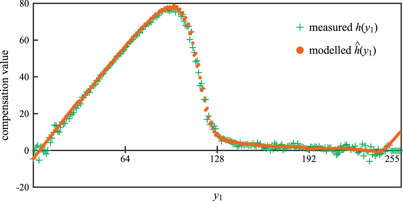
Figure 7 illustrates the compensation values  $h(y_1)$ and $\hat {h}(y_1)$ of the measured and modeled cases calculated by (22) and (23), respectively. The size of input image shown in Fig. 2(a) is $471 \times 640$ (pixels), and 8 bit depth (256 tones) grayscale. In the measured case, the data size to be included in the overhead information is about 2.4 million bits. On the other hand, in the modeled case, that is about 16 thousand bits. Note that, it is assumed that histogram information expresses each tone by the Double type (64 bits). The overhead information in the modeled case is greatly less than the measured case. Thus, the modeled case makes it possible to greatly reduce the data size to be included in the overhead information while maintaining the measured case quality.
Noise bias compensation values.
IV. EXPERIMENTAL RESULTS
NBC in this paper classifies pixels in the noisy image into several subsets according to the observed pixel value, and compensates the pixel value in each subset with a preliminarily determined compensation value. Based on the Bayesian inference theory, the compensation value is determined from the histogram of pixel values in an image and that of the noise before TM. In NBC, for each image, the compensation value corresponding to that image is automatically calculated. This section confirms effectiveness of the proposed method experimentally.
A) Effect of NBC
Figure 8 illustrates the NB before and after TM for the input image shown in Fig. 2(a). For pixel values with small values, the noise bias is greatly reduced. For small pixel values, the noise bias is greatly reduced. This means that the NBC has a large effect on compensation of small pixel values. Table 1 summarizes the average and variance of NB. After NBC, the variance is greatly reduced, and the average is approaching zero value.
NB before and after NBC for the input image shown in Fig. 2(a).
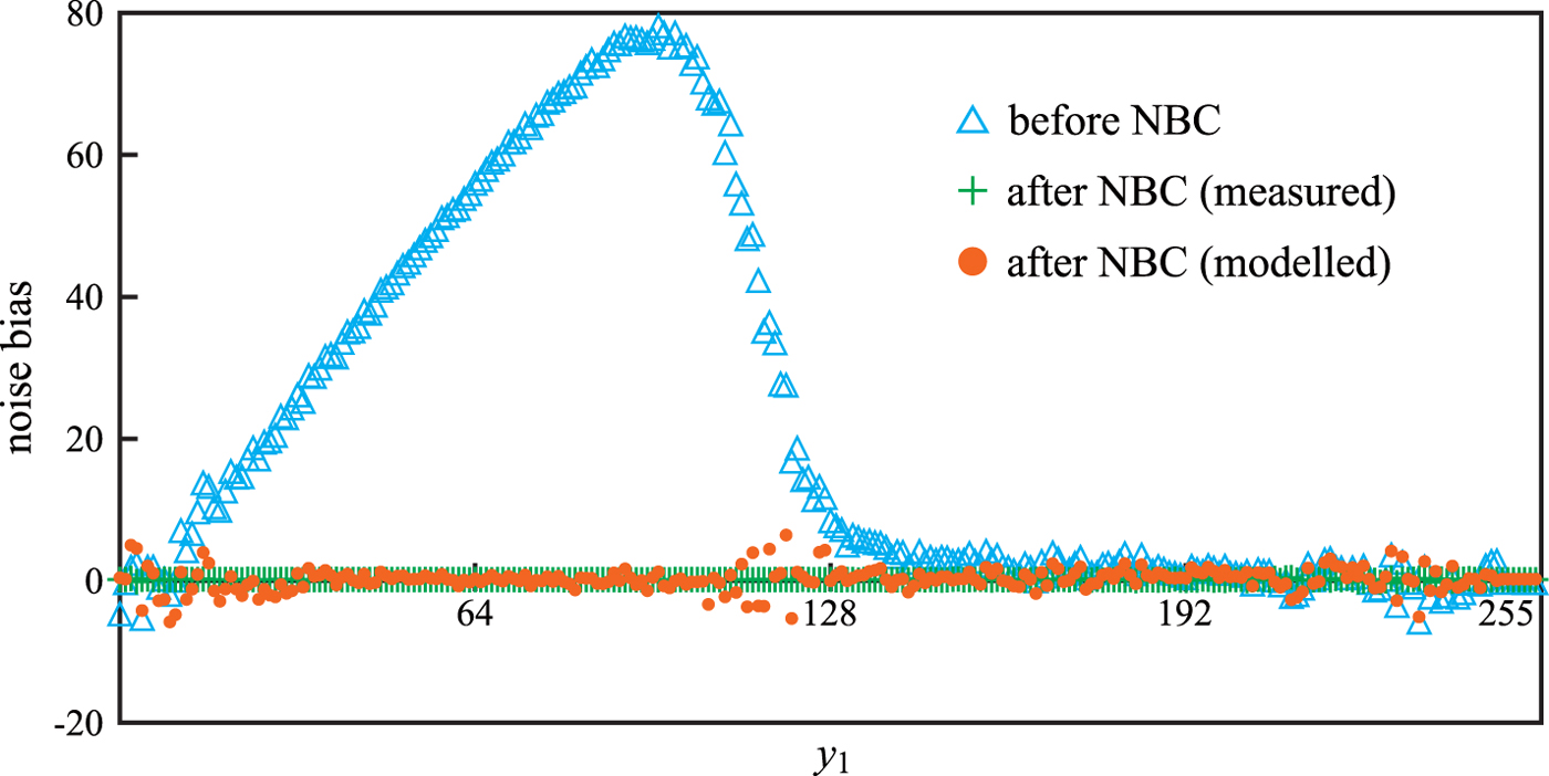
Average and variance of all NB shown in Fig. 8.

B) Quality of compensated images
The image quality before and after NBC is evaluated with the peak signal to noise ratio (PSNR) defined as
 $$PSNR = 10 \log_{10} { Y_{MAX}^2 \over{Var}[\delta({\bf{n}})]}.$$
Figure 9 illustrates comparison of PSNR before and after NBC for the input image shown in Fig. 2(a). Figures 9(a) and 9(b) investigate the effect of γ in the TM function in (3) and that of σ in the PMF of noise in (6), respectively. It is observed that the image quality after NBC is improved. In Figs 9(a) and 9(b), the modeled NBC is only 0.0053 (dB) and 0.0197 (dB) lower than the measured on average respectively, and there is no significant difference.
PSNR of the compensated image. (a) Effect of γ ( $\sigma = 8$), (b) effect of σ ( $\gamma = 3$).

C) Combination with non-local mean filter
This section investigates combination of NBC and NLM filter. In the NLM filter used in the experiment, the sizes of the search window and the similarity window were set to  $3\times 3$ and
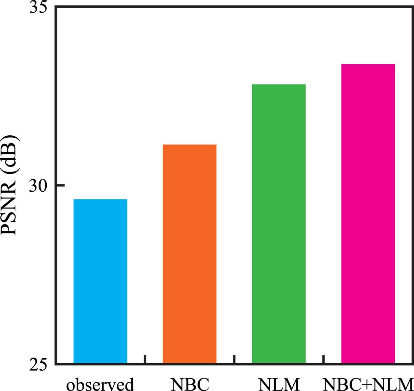
  $2\times 2$, respectively. The CVC-14 dataset [Reference González, Fang, Socarras, Serrat, Vázquez and López35] that has 4072 night scene images gathered using visible cameras were used as test images. In addition, 16 astronomical images randomly selected from the NASA Image and Video Library [36] were used as well. Figure 10 illustrates experimental results of comparison of the average PSNR of all night scene images in the CVC-14 dataset. The average of NBC is 1.68 (dB) lower than that of NLM. However, in about $20\%$ of all night scene images, NBC is superior to NLM. The average of NBC+NLM is 0.94 (dB) higher than that of NLM. In the best results, NBC+NLM is 3.37 (db) higher than NLM. In about
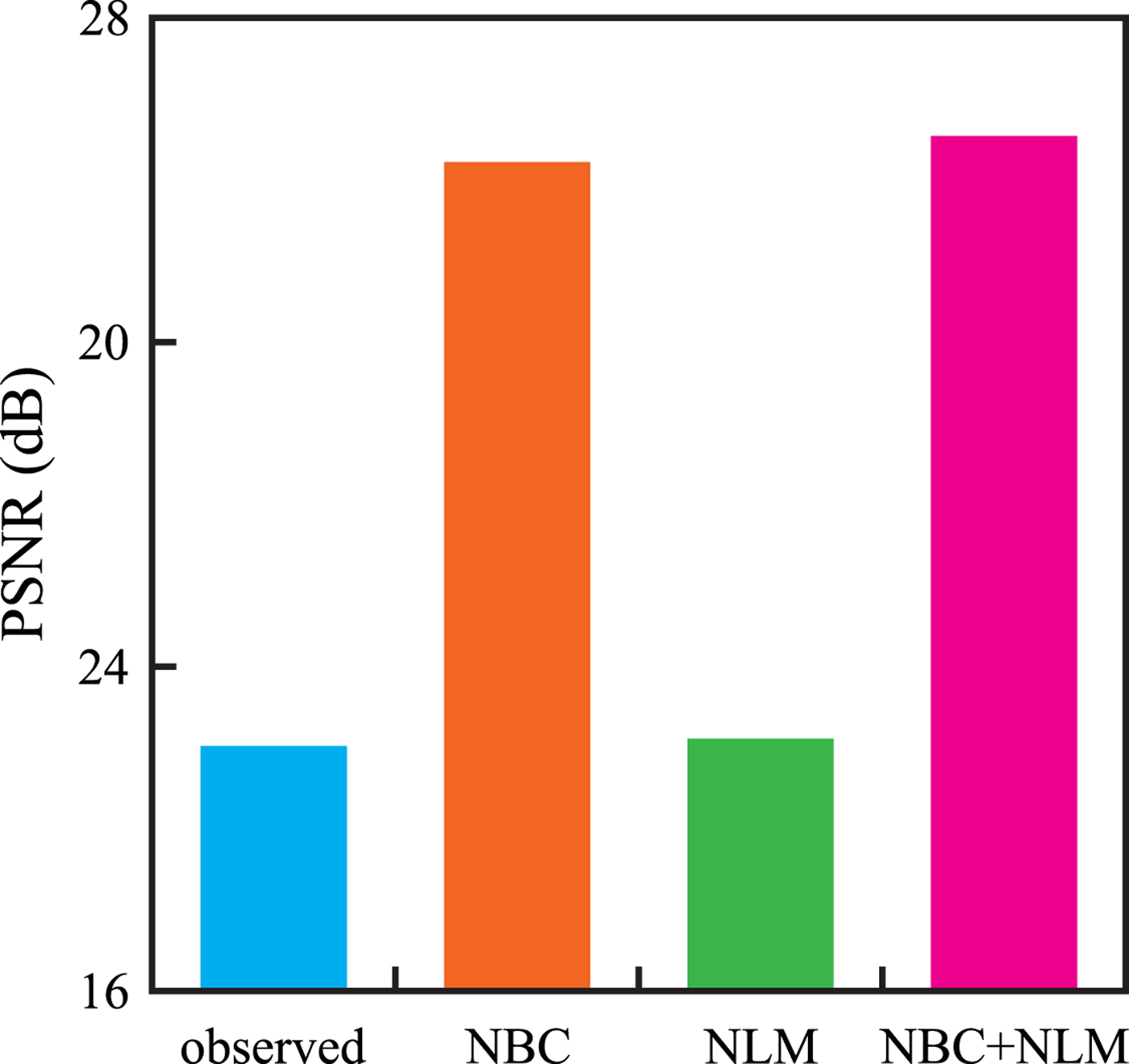
  $80\%$ of all night scene images, NBC+NLM is superior to NLM. Figure 11 illustrates experimental results of comparison of the average PSNR of astronomical images. The average of NBC is 7.11 (dB) higher than that of NLM. The average of NBC+NLM is 7.43 (dB) higher than that of NLM. Denoising performance is improved by combination. This means that NBC can coexist with approaches focusing on the correlation between pixels like NLM filter. In addition, NBC is effective as preprocessing such as NLM filter.
The average PSNR of the compensated and filtered images for the CVC-14 dataset.  $\gamma =3$, $\sigma =8$. Note that “observed”, “NLM”, “NBC”, and“NBC+NLM” indicate the observed image, the image after NLM filter, the image after NBC (the modeled case), and the combination of NBC (the modeled case) and NLM filter, respectively.
The average PSNR of the compensated and filtered images for astronomical images.  $\gamma =3$, $\sigma =8$.
Result images after NBC, NLM filter, and NBC+NLM are illustrated in Figs 12 and 13. Compared with NLM, noise was reduced in NBC and NBC+NLM. NBC has a large effect on compensation of small pixel values. Therefore, in the TM of a dark image like night scene images, NBC is a great effect on denoising.
Results of NBC, NLM, and NBC+NLM for the image shown in Fig. 2(a). PSNR of observed output is 28.13 (dB). (a) NBC (29.99 dB), (b) NLM (30.13 dB), (c) NBC+NLM (32.45 dB).

Results of NBC, NLM, and NBC+NLM for an astronomical image. (a) Input image, (b) ideal output image, (c) input noise  $(\sigma = 8)$, (d) noisy image, (e) observed output image (16.15 dB), (f) NBC (21.52 dB), (g) NLM (16.15 dB), (h) NBC+NLM (21.65 dB).

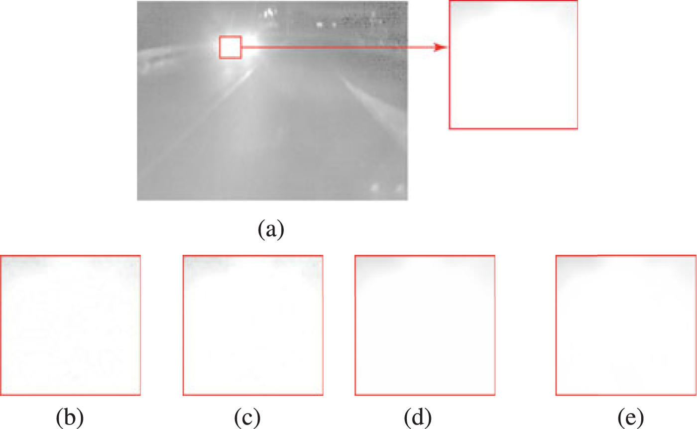
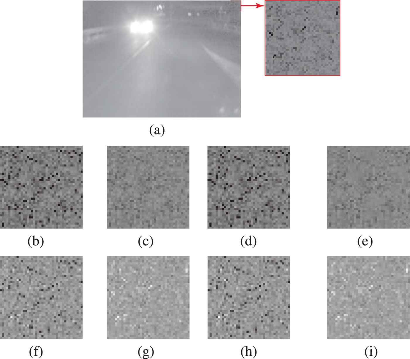
Figure 14 illustrates details of the bright area. There is no difference in all images. Figure 15 illustrates details of the dark area. NLM is similar to the observed image, and these are noisy. On the other hand, NBC and NBC+NLM are not noisy, and improvement of image quality is confirmed. TM function in (3), when  $\gamma >1$, the gradient is steep as the pixel value is smaller as shown in Fig. 6(a). Moreover, when the pixel value is small, the absolute value of NB is large (= large bias), as shown in Fig. 7. Therefore, significant effects can be obtained in the dark area. On the other hand, when the pixel value is large, NB is close to zero value (= no bias). Therefore, no significant effects can be obtained in the bright area.
Detailed results of the bright place. (a) Reference (ideal output image), (b) observed, (c) NBC, (d) NLM, (e) NBC+NLM.
Detailed results of the dark place. (f)–(i) Output noise. (a) Reference (ideal output image), (b) observed, (c) NBC, (d) NLM, (e) NBC+NLM, (f)observed, (g) NBC, (h) NLM, (i) NBC+NLM.
V. CONCLUSIONS
In this paper, NBC method for tone mapped noisy image was proposed. The compensation value is calculated using the prior knowledge. The effectiveness of the proposed method over the existing method was experimentally confirmed for several tone mapped noisy LDR images. It was experimentally confirmed that the combination of NBC and approaches focusing on the correlation between pixels like NLM filter improved the denoising performance more than when only either one was used. The advantage of the denoising performance was confirmed by using NBC as preprocessing for NLM filter. NBC is not an approach focusing on the correlation between pixels, and NBC can coexist with approaches focusing on the correlation between pixels like NLM filter. Noise with other probability distributions, such as shot noise with the Poisson distribution, and single domain or global information-based should be investigated in the future. In addition, we should analyze the effectiveness of combinations with various filters other than NLM in future work.
FINANCIAL SUPPORT
This work was supported by JSPS KAKENHI Grant Number 16K13715.
Sayaka Minewaki received her B.Eng. and M.Eng. degrees in Engineering from Kyushu Institute of Technology in 2001 and 2003, respectively. In 2006, she finished a Ph.D. program without dissertation at the Department of Artificial Intelligence, Kyushu Institute of Technology. In 2006, she joined Department of Computer Science and Engineering, National Institute of Technology, Yuge College, where she served concurrently as a Lecturer. From 2016 to 2018, she joined Nagaoka University of Technology, where she is currently an Assistant Professor of the Department of Electrical, Electronics and Information Engineering. From 2018, she has been with the Department of Computer Science and Engineering, National Institute of Technology, Yuge College. Her research interests are in the fields of digital signal processing, image compression, and natural language processing.
Taichi Yoshida received B.Eng., M.Eng, and Ph.D. degrees in Engineering from Keio University, Yokohama, Japan, in 2006, 2008, and 2013. In 2014, he joined Nagaoka University of Technology, where he is currently an Assistant Professor in the Department of Electrical, Electronics and Information Engineering, Faculty of Technology. His research interests are in the field of filter bank design, image coding, and image processing.
Yoshinori Takei received the B.Sc. and M.Sc. degrees in mathematics in 1990 and 1992, respectively, from Tokyo Institute of Technology and the Dr. Eng. degree in information processing in 2000, from Tokyo Institute of Technology, Yokohama, Japan. From 1992 to 1995, he was with Kawasaki Steel System R&D Inc., Chiba, Japan. From 1999 to 2000, he was an Assistant Professor with the Department of Electrical and Electronic Engineering, Tokyo Institute of Technology. From 2000 to 2017, he was with the Department of Electrical Engineering, Nagaoka University of Technology, Niigata, Japan, where he was finally an Associate Professor. From 2017, he has been withthe Department of Electrical and Computer Engineering, National Institute of Technology, Akita College, where he is an Associate Professor. His current research interests include computational complexity theory, public-key cryptography, randomized algorithms, and digital signal processing. Especially, he is now interested in the application of non-commutative harmonic analysis to data-mining. Dr. Takei is a member of LA, SIAM, ACM, AMS, and IEICE.
Masahiro Iwahashi received his B.Eng, M.Eng., and D.Eng. degrees in electrical engineering from Tokyo Metropolitan University in 1988, 1990, and 1996, respectively. In 1990, he joined Nippon Steel Co. Ltd.. From 1991 to 1992, he was dispatched to Graphics Communication Technology Co. Ltd.. In 1993, he joined Nagaoka University of Technology, where he is currently a professor of Department of Electrical Engineering, Faculty of Technology. From 1995 to 2001, he served concurrently as a lecturer of Nagaoka Technical College. From 1998 to 1999, he dispatched to Thammasat University in Bangkok, Thailand as a JICA expert. His research interests are in the area of digital signal processing, multi-rate systems, image compression. From 2007 to 2011, he served as an editorial committee member of the transaction on fundamentals. He is serving as a reviewer of IEEE, IEICE, and APSIPA. He is currently a senior member of the IEEE and IEICE.
Hitoshi Kiya received his B.E and M.E. degrees from Nagaoka University of Technology, in 1980 and 1982 respectively, and his Dr. Eng. degree from Tokyo Metropolitan University in 1987. In 1982, he joined Tokyo Metropolitan University, where he became Full Professor in 2000. He is a Fellow of IEEE, IEICE, and ITE. He currently serves as President of APSIPA (2019–2020), and served as Inaugural Vice President (Technical Activities) of APSIPA from 2009 to 2013, Regional Directorat-Large for Region 10 of the IEEE Signal Processing Society from 2016 to 2017. He was Editorial Board Member of eight journals, including IEEE Transactions on Signal Processing, Image Processing, and Information Forensics and Security, Chair of two technical committees and Member of nine technical committees including APSIPA Image, Video, and Multimedia TC, and IEEE Information Forensics and Security TC. Kiya was a recipient of numerous awards, including six best paper awards.


 Open access