


1. Introduction
In a recent study (Guo, Taylor & Zhou (Reference Guo, Taylor and Zhou2024), hereafter referred to as G24), we investigated the linear stability properties of columnar Taylor–Green (TG) vortices under strong stratification, specifically for Froude number $ 0.125\leqslant \textit{Fr} \leqslant 1.0$
and Reynolds number
$ 0.125\leqslant \textit{Fr} \leqslant 1.0$
and Reynolds number ${\textit{Re}}=1600$
. The focus was on identifying and understanding the primary instability that leads to the breakdown of these freely evolving vortices. Our analysis revisited the instability mechanism of the most unstable eigenmode, previously identified by Hattori et al. (Reference Hattori, Suzuki, Hirota and Khandelwal2021) as the mixed hyperbolic mode, and revealed its similarity to the well-known zigzag instability. We found that the primary linear instability of TG vortices exhibits a fastest-growing wavenumber (when non-dimensionalised) that is inversely proportional to
${\textit{Re}}=1600$
. The focus was on identifying and understanding the primary instability that leads to the breakdown of these freely evolving vortices. Our analysis revisited the instability mechanism of the most unstable eigenmode, previously identified by Hattori et al. (Reference Hattori, Suzuki, Hirota and Khandelwal2021) as the mixed hyperbolic mode, and revealed its similarity to the well-known zigzag instability. We found that the primary linear instability of TG vortices exhibits a fastest-growing wavenumber (when non-dimensionalised) that is inversely proportional to ${\textit{Fr}}$
and maintains an approximately constant dimensionless growth rate with
${\textit{Fr}}$
and maintains an approximately constant dimensionless growth rate with ${\textit{Fr}}$
, consistent with zigzag instability originally observed in a vortex pair by Billant & Chomaz (Reference Billant and Chomaz2000a
,
Reference Billant and Chomazb
,
Reference Billant and Chomazc
). Since then, Billant, Chomaz and their co-workers made numerous seminal contributions towards the theory, experimental validation and numerical investigation of this generic instability and its transition to turbulence (e.g. Deloncle et al. Reference Deloncle, Billant and Chomaz2008, Reference Deloncle, Billant and Chomaz2011; Augier & Billant Reference Augier and Billant2011; Augier, Chomaz & Billant Reference Augier, Chomaz and Billant2012). Dimensionally, the scaling relations for the zigzag instability feature a dominant wavelength that scales with
${\textit{Fr}}$
, consistent with zigzag instability originally observed in a vortex pair by Billant & Chomaz (Reference Billant and Chomaz2000a
,
Reference Billant and Chomazb
,
Reference Billant and Chomazc
). Since then, Billant, Chomaz and their co-workers made numerous seminal contributions towards the theory, experimental validation and numerical investigation of this generic instability and its transition to turbulence (e.g. Deloncle et al. Reference Deloncle, Billant and Chomaz2008, Reference Deloncle, Billant and Chomaz2011; Augier & Billant Reference Augier and Billant2011; Augier, Chomaz & Billant Reference Augier, Chomaz and Billant2012). Dimensionally, the scaling relations for the zigzag instability feature a dominant wavelength that scales with $U_0/N$
, and a growth rate that scales with
$U_0/N$
, and a growth rate that scales with $U_0/L$
, where
$U_0/L$
, where $U_0$
and
$U_0$
and $L$
are the characteristic velocity and length scales, and
$L$
are the characteristic velocity and length scales, and $N$
is the buoyancy frequency. As such, the TG vortex array undergoing zigzag instability may directly transfer its kinetic energy into stratified turbulence at a specific vertical length scale, forming a crucial link in the hypothesised energy pathway of stratified geophysical flows (Augier et al. Reference Augier, Chomaz and Billant2012; Waite Reference Waite2013).
$N$
is the buoyancy frequency. As such, the TG vortex array undergoing zigzag instability may directly transfer its kinetic energy into stratified turbulence at a specific vertical length scale, forming a crucial link in the hypothesised energy pathway of stratified geophysical flows (Augier et al. Reference Augier, Chomaz and Billant2012; Waite Reference Waite2013).
Previous studies have extensively examined the onset of turbulence due to zigzag instability in a vortex pair (Deloncle, Billant & Chomaz Reference Deloncle, Billant and Chomaz2008; Waite & Smolarkiewicz Reference Waite and Smolarkiewicz2008; Augier & Billant Reference Augier and Billant2011). Two mechanisms have been proposed for the transition to turbulence: shear driven and gravitationally driven (i.e. convection). Deloncle et al. (Reference Deloncle, Billant and Chomaz2008) considered the turbulence transition to be shear driven, arguing that turbulence would not be triggered if the spontaneously formed vertical shear layers are directly subject to viscous effects. This argument leads to a viscous scaling for the local gradient Richardson number $Ri$
, based on the Reynolds and Froude numbers of the vortex pair, i.e.
$Ri$
, based on the Reynolds and Froude numbers of the vortex pair, i.e. $Ri \propto 1/({\textit{Re}}\, {\textit{Fr}}^2)$
. For the shear layers to become unstable,
$Ri \propto 1/({\textit{Re}}\, {\textit{Fr}}^2)$
. For the shear layers to become unstable, $Ri$
must be sufficiently small, implying that
$Ri$
must be sufficiently small, implying that ${\textit{Re}}\, {\textit{Fr}}^2$
must exceed a certain threshold. In contrast, Waite & Smolarkiewicz (Reference Waite and Smolarkiewicz2008) characterised the turbulence transition as gravitationally driven (see e.g. their figure 10), finding that density overturns occur only when
${\textit{Re}}\, {\textit{Fr}}^2$
must exceed a certain threshold. In contrast, Waite & Smolarkiewicz (Reference Waite and Smolarkiewicz2008) characterised the turbulence transition as gravitationally driven (see e.g. their figure 10), finding that density overturns occur only when ${\textit{Re}}\, {\textit{Fr}}$
is sufficiently large. Augier & Billant (Reference Augier and Billant2011) reconciled these two perspectives, suggesting that both mechanisms can occur simultaneously for a vortex pair undergoing the primary zigzag instability. In the present study, we will extend the analysis of the turbulence onset due to zigzag instability from a vortex pair to a vortex array. Our first aim is to determine whether the same mechanisms observed for the vortex pair apply to the TG vortex array, and identify the region in the
${\textit{Re}}\, {\textit{Fr}}$
is sufficiently large. Augier & Billant (Reference Augier and Billant2011) reconciled these two perspectives, suggesting that both mechanisms can occur simultaneously for a vortex pair undergoing the primary zigzag instability. In the present study, we will extend the analysis of the turbulence onset due to zigzag instability from a vortex pair to a vortex array. Our first aim is to determine whether the same mechanisms observed for the vortex pair apply to the TG vortex array, and identify the region in the ${\textit{Re}}$
–
${\textit{Re}}$
– ${\textit{Fr}}$
parameter space where the flow is expected to become turbulent (or not).
${\textit{Fr}}$
parameter space where the flow is expected to become turbulent (or not).
Stratified turbulence is often associated with the formation of vertical layers of momentum (shear) or buoyancy. Riley & de Bruyn Kops (Reference Riley and de Bruyn Kops2003) performed direct numerical simulations (DNS) of three-dimensional (3-D) TG vortices (different from the columnar vortices in this study) and observed layering in the mean vertical shear of horizontal velocity (see their figures 3 and 4). Brethouwer et al. (Reference Brethouwer, Billant, Lindborg and Chomaz2007) proposed the scalings for the characteristic vertical length of these layers based on their DNS where only vertically invariant modes were forced. These scalings have been verified in other contexts, such as in decaying stratified wake turbulence (Zhou & Diamessis Reference Zhou and Diamessis2019). Additional evidence for shear layering has emerged from recent studies on horizontally sheared flows (Lucas et al. Reference Lucas, Caulfield and Kerswell2017, Reference Lucas, Caulfield and Kerswell2019; Lewin & Caulfield Reference Lewin and Caulfield2024). Experiments on stably stratified fluids stirred by horizontally moving objects have also demonstrated the layering of density (see e.g. Park, Whitehead & Gnanadeskian Reference Park, Whitehead and Gnanadeskian1994; Holford & Linden Reference Holford and Linden1999), which has been explored through theoretical models (Balmforth, Llewellyn Smith & Young Reference Balmforth, Llewellyn Smith and Young1998; Taylor & Zhou Reference Taylor and Zhou2017). It is worth noting that the vortical structure (see figure 6 of Praud, Fincham & Sommeria Reference Praud, Fincham and Sommeria2005) in the initial wake generated by a horizontally towed rake of vertical plates indeed resembles an array of columnar vertical vortices, the latter being the focus of the present study. While the dynamical origin of layering is relatively better understood in flows involving multiple active scalars, such as double-diffusive convection (e.g. Pružina et al. Reference Pružina, Zhou, Middleton and Taylor2025), the understanding remains more limited for configurations with a single active scalar. Numerical observations of the self-sharpening of density interfaces in such cases are largely restricted to a few examples (Taylor & Zhou Reference Taylor and Zhou2017; Zhou et al. Reference Zhou, Taylor, Caulfield and Linden2017) with vertically sheared flows that were initialised specifically to promote layer formation, i.e. under somewhat contrived conditions. Given that the mechanisms driving the layering of momentum and buoyancy are not fully understood, our second aim is to investigate whether and how the zigzag instability of vortex arrays may contribute to layering in stratified fluids.
Our current work is thus motivated by several questions aimed at deepening our understanding of the stratified turbulence generated by zigzag instability of columnar vortex arrays. Through the DNS conducted in G24, we observed that while the stability analysis suggests that the TG vortices are linearly unstable, the zigzag instability does not always generate vigorous turbulence in the flow (see e.g. figure 9 of G24). This is likely due to strong stratification, a prerequisite for the zigzag instability, which may inhibit the onset of turbulence. The first key question is: under what conditions does the TG vortex array trigger turbulence, and when it does, which mechanism drives the transition to turbulence – is it shear or convection? Second, since the zigzag instability injects energy at a specific vertical length scale, what are the structural implications for the stratified turbulence triggered by this process? Could the breakdown of zigzag instability in columnar TG vortices, a vertically invariant base flow, lead to the vertical layering of shear and density? And if so, how do the characteristics of these post-instability layers compare to those of the instability itself?
The objectives of this paper are to address the aforementioned questions by examining the conditions under which zigzag instability transitions to turbulence in TG vortices, identifying the transition mechanisms, and exploring the structural changes induced by zigzag instability, such as layering of shear and buoyancy. The remainder of the paper is organised as follows. In § 2, we introduce the DNS data set under examination. In § 3.1, the mechanisms for the onset of turbulence are discussed, and in § 3.2, the parametric dependence on ${\textit{Re}}$
and
${\textit{Re}}$
and ${\textit{Fr}}$
is investigated. In § 4, we focus on the phenomena of layering (of shear in § 4.1 and buoyancy in § 4.2). In § 5, we offer concluding remarks.
${\textit{Fr}}$
is investigated. In § 4, we focus on the phenomena of layering (of shear in § 4.1 and buoyancy in § 4.2). In § 5, we offer concluding remarks.
2. The DNS
We consider the dimensionless, incompressible Navier–Stokes equations under the Boussinesq approximation:
 \begin{align}& \frac {\partial {\boldsymbol{u}}}{\partial {t}} +\boldsymbol{u} \boldsymbol{\boldsymbol{\cdot}} \boldsymbol{\nabla} \boldsymbol{u} =-{\boldsymbol{\nabla} } {\Pi} +\frac {1}{\textit{Re}}{\nabla} ^2 \boldsymbol{u} - \frac {1}{{\textit{Fr}}^2}\rho \hat {\boldsymbol{k}}, \end{align}
 \begin{align}&\qquad\qquad\qquad\quad \mathbf{\boldsymbol{\nabla} } \boldsymbol{\boldsymbol{\cdot}} \boldsymbol{u} =0, \end{align}
 \begin{align}&\qquad\,\, \frac {\partial {\rho }}{\partial {t}} +\boldsymbol{u}\boldsymbol{\boldsymbol{\cdot}} \mathbf{\boldsymbol{\nabla} } \rho -w =\frac {1}{{\textit{Re}}\, Pr}\nabla ^2\rho , \end{align}
where $\boldsymbol{u}=(u,v,w)$
is the fluid velocity,
$\boldsymbol{u}=(u,v,w)$
is the fluid velocity, $\Pi$
is the pressure deviation from the hydrostatic balance, and
$\Pi$
is the pressure deviation from the hydrostatic balance, and $\rho$
is the perturbation density to a constant background stratification. The Prandtl number
$\rho$
is the perturbation density to a constant background stratification. The Prandtl number $Pr$
is set to 0.7 throughout this paper. The Reynolds and Froude numbers are defined as
$Pr$
is set to 0.7 throughout this paper. The Reynolds and Froude numbers are defined as
 \begin{equation} {\textit{Re}}= \frac {U_0L}{\nu }, \quad \textit{Fr} = \frac {U_0}{N L}, \end{equation}
where $N$
is the constant background buoyancy frequency,
$N$
is the constant background buoyancy frequency, $\nu$
is the kinematic viscosity, and
$\nu$
is the kinematic viscosity, and $U_0$
and
$U_0$
and $L$
represent the velocity and length scales, respectively. Specifically,
$L$
represent the velocity and length scales, respectively. Specifically, $U_0$
and
$U_0$
and $L$
are chosen such that the dimensionless velocity field in the TG base flow is written as
$L$
are chosen such that the dimensionless velocity field in the TG base flow is written as
 \begin{equation} (\sin x \cos y, -\cos x\sin y, 0) \end{equation}
for $x,y\in [0,2\unicode{x03C0})$
. Such a base flow features a two-by-two array of columnar vortices, as illustrated in figure 1 of G24.
$x,y\in [0,2\unicode{x03C0})$
. Such a base flow features a two-by-two array of columnar vortices, as illustrated in figure 1 of G24.
We conducted DNS of the columnar TG vortices using the numerical configuration detailed in G24. Validation of the numerical code is provided in Guo, Zhou & Wong (Reference Guo, Zhou and Wong2023) and in Appendix B of G24. The DNS were performed in a triply periodic domain with length $2\unicode{x03C0}$
in each direction. The initial condition for the simulation is the base flow (2.3) weakly perturbed by random noise (see (3.1) of G24). The parameters of the DNS are summarised in table 1. The simulations for
$2\unicode{x03C0}$
in each direction. The initial condition for the simulation is the base flow (2.3) weakly perturbed by random noise (see (3.1) of G24). The parameters of the DNS are summarised in table 1. The simulations for ${\textit{Re}}=1600$
and
${\textit{Re}}=1600$
and $0.125\leqslant {\textit{Fr}}\leqslant 1.0$
were those considered in G24, while the present study includes additional simulations for two other
$0.125\leqslant {\textit{Fr}}\leqslant 1.0$
were those considered in G24, while the present study includes additional simulations for two other ${\textit{Re}}$
values, 800 and 3200. The resolution is chosen such that the grid spacing is no more than approximately 2.2 times the Kolmogorov scale (see table 1). Following the approach in G24, we performed linear stability analysis (LSA) for all cases listed in table 1, confirming that zigzag instability is the most unstable linear mode for the base flow within the investigated ranges of
${\textit{Re}}$
values, 800 and 3200. The resolution is chosen such that the grid spacing is no more than approximately 2.2 times the Kolmogorov scale (see table 1). Following the approach in G24, we performed linear stability analysis (LSA) for all cases listed in table 1, confirming that zigzag instability is the most unstable linear mode for the base flow within the investigated ranges of ${\textit{Re}}$
and
${\textit{Re}}$
and ${\textit{Fr}}$
. While we covered four values of
${\textit{Fr}}$
. While we covered four values of ${\textit{Fr}}$
between 0.25 and 2.0 at
${\textit{Fr}}$
between 0.25 and 2.0 at ${\textit{Re}}=3200$
, we were unable to simulate the case
${\textit{Re}}=3200$
, we were unable to simulate the case $({\textit{Re}},{\textit{Fr}})=(3200,0.125)$
because the computational cost exceeded what was accessible to us.
$({\textit{Re}},{\textit{Fr}})=(3200,0.125)$
because the computational cost exceeded what was accessible to us.
Summary of DNS parameters: $(N_x,N_y,N_z)$
are the numbers of grid points used in each direction,
$(N_x,N_y,N_z)$
are the numbers of grid points used in each direction, $h$
is the grid spacing,
$h$
is the grid spacing, $\eta _{\textit{min}}$
is the minimum Kolmogorov scale at peak dissipation,
$\eta _{\textit{min}}$
is the minimum Kolmogorov scale at peak dissipation, $\Delta t$
is the time step size,
$\Delta t$
is the time step size, ${\textit{Re}}_b^\star$
is the peak value of the buoyancy Reynolds number, and
${\textit{Re}}_b^\star$
is the peak value of the buoyancy Reynolds number, and ${\textit{Fr}}_t^\star$
is the maximum turbulent Froude number. Both
${\textit{Fr}}_t^\star$
is the maximum turbulent Froude number. Both ${\textit{Re}}_b^\star$
and
${\textit{Re}}_b^\star$
and ${\textit{Fr}}_t^\star$
are discussed in § 3.2.
${\textit{Fr}}_t^\star$
are discussed in § 3.2.

3. Transition to turbulence
3.1. Transition mechanism
We begin by examining the flow evolution for the case where $({\textit{Re}}, {\textit{Fr}}) = (1600, 1.0)$
, with a focus on the onset of turbulence and its driving mechanisms. Figure 1 shows the evolution of the vertical vorticity, highlighting key stages in the flow’s development. As the initial, weak disturbances to the base flow grow via zigzag instability, the columnar vortices become visibly distorted by
$({\textit{Re}}, {\textit{Fr}}) = (1600, 1.0)$
, with a focus on the onset of turbulence and its driving mechanisms. Figure 1 shows the evolution of the vertical vorticity, highlighting key stages in the flow’s development. As the initial, weak disturbances to the base flow grow via zigzag instability, the columnar vortices become visibly distorted by $t \leqslant 44$
, introducing variations in the vertical direction. By
$t \leqslant 44$
, introducing variations in the vertical direction. By $t = 48$
, localised, intense patches of prolonged vortical structures, which we will consider as the finite-amplitude manifestation of the primary zigzag instability, appear between the vortex columns and quickly trigger turbulence. The turbulence reaches its peak intensity by
$t = 48$
, localised, intense patches of prolonged vortical structures, which we will consider as the finite-amplitude manifestation of the primary zigzag instability, appear between the vortex columns and quickly trigger turbulence. The turbulence reaches its peak intensity by $t = 56$
, and subsequently decays over time as the initial columnar vortices disappear completely.
$t = 56$
, and subsequently decays over time as the initial columnar vortices disappear completely.
Volume-rendering images of the vertical vorticity field $\omega _z=\partial v/ \partial x- \partial u/ \partial y$
, from the DNS with
$\omega _z=\partial v/ \partial x- \partial u/ \partial y$
, from the DNS with ${\textit{Re}}=1600$
and
${\textit{Re}}=1600$
and ${\textit{Fr}}=1.0$
. The first image in the sequence was captured at time
${\textit{Fr}}=1.0$
. The first image in the sequence was captured at time $t=36$
. Subsequent images are spaced at regular intervals of 4.0 units of time, arranged from left to right and top to bottom. An animation of the flow evolution can be found as movie 1 in the supplementary movies available at https://doi.org/10.1017/jfm.2025.10420.
$t=36$
. Subsequent images are spaced at regular intervals of 4.0 units of time, arranged from left to right and top to bottom. An animation of the flow evolution can be found as movie 1 in the supplementary movies available at https://doi.org/10.1017/jfm.2025.10420.

In figure 2, we analyse the evolution of the vertically averaged and fluctuating components of kinetic energy. The flow field $\boldsymbol{u}=(u,v,w)$
is decomposed into the vertically averaged component
$\boldsymbol{u}=(u,v,w)$
is decomposed into the vertically averaged component $\overline {\boldsymbol{U}} = (\overline {U}, \overline {V}, 0)$
and the fluctuation
$\overline {\boldsymbol{U}} = (\overline {U}, \overline {V}, 0)$
and the fluctuation $\boldsymbol{u}' = (u', v', w')$
. The vertically invariant and fluctuating kinetic energy are defined as
$\boldsymbol{u}' = (u', v', w')$
. The vertically invariant and fluctuating kinetic energy are defined as
 \begin{equation} \overline {E}_k = \tfrac {1}{2} \langle \overline {\mathbf U} \boldsymbol{\boldsymbol{\cdot}} \overline {\mathbf U} \rangle , \quad E_k^{\prime} = \tfrac {1}{2} \langle \mathbf u' \boldsymbol{\boldsymbol{\cdot}} \mathbf u' \rangle , \end{equation}
where $\langle {\boldsymbol{\cdot}} \rangle \equiv (2\unicode{x03C0} )^{-3} \iiint ({\boldsymbol{\cdot}} )\, \mathrm{d}x\, \mathrm{d}y\, \mathrm{d}z$
denotes the volume average over the 3-D domain. Figure 2(a) shows that the vertically invariant component
$\langle {\boldsymbol{\cdot}} \rangle \equiv (2\unicode{x03C0} )^{-3} \iiint ({\boldsymbol{\cdot}} )\, \mathrm{d}x\, \mathrm{d}y\, \mathrm{d}z$
denotes the volume average over the 3-D domain. Figure 2(a) shows that the vertically invariant component $\overline {E}_k$
dominates the kinetic energy for
$\overline {E}_k$
dominates the kinetic energy for $t \lesssim 40$
. After this point, the vertically varying component grows rapidly, extracting energy from the vertically uniform background flow. In figure 2(b), where
$t \lesssim 40$
. After this point, the vertically varying component grows rapidly, extracting energy from the vertically uniform background flow. In figure 2(b), where $E_k^{\prime}$
is replotted on a logarithmic scale, its linear growth can be observed approximately between
$E_k^{\prime}$
is replotted on a logarithmic scale, its linear growth can be observed approximately between $t = 15$
and
$t = 15$
and $t=45$
. Figure 2(c) plots the volume-averaged kinetic energy pseudo-dissipation rate
$t=45$
. Figure 2(c) plots the volume-averaged kinetic energy pseudo-dissipation rate $\varepsilon _k = \langle \epsilon _k \rangle$
, where
$\varepsilon _k = \langle \epsilon _k \rangle$
, where
 \begin{equation} \epsilon _k = \frac {1}{\textit{Re}} \frac {\partial {u_i}}{\partial {x_j}} \frac {\partial {u_i}}{\partial {x_j}}. \end{equation}
As is common in similar numerical studies (e.g. Lucas, Caulfield & Kerswell Reference Lucas, Caulfield and Kerswell2019; Howland, Taylor & Caulfield Reference Howland, Taylor and Caulfield2020), pseudo-dissipation is used in place of the full dissipation rate from the turbulent kinetic energy budget (see e.g. equation 1 in Caulfield Reference Caulfield2021) for ease of computation. The value of $\varepsilon _k$
reaches its peak at
$\varepsilon _k$
reaches its peak at $t \approx 56$
, shortly after the fluctuating kinetic energy
$t \approx 56$
, shortly after the fluctuating kinetic energy $E_k^{\prime}$
reaches its maximum at
$E_k^{\prime}$
reaches its maximum at $t \approx 54$
.
$t \approx 54$
.
Time series of (a,b) kinetic energy components and (c) dissipation rate for the case with ${\textit{Re}}=1600$
and
${\textit{Re}}=1600$
and ${\textit{Fr}} = 1.0$
. Circles in (b,c) correspond to
${\textit{Fr}} = 1.0$
. Circles in (b,c) correspond to $t=40$
, 44 and 48.
$t=40$
, 44 and 48.

To understand the mechanisms behind the onset of turbulence, we focus on three specific time instances: $t=40$
,
$t=40$
, $44$
and
$44$
and $48$
, which are marked with circles in figure 2(b,c). During these times, the primary instability is approaching the end of its linear growth phase, as indicated in figure 2(b). At the same time, the dissipation is beginning to increase significantly, as shown in figure 2(c). Additional visualisations of these instances are provided in figure 3, where the isosurfaces of vertical vorticity are plotted (in red and blue) in conjunction with regions that are convectively unstable, i.e.
$48$
, which are marked with circles in figure 2(b,c). During these times, the primary instability is approaching the end of its linear growth phase, as indicated in figure 2(b). At the same time, the dissipation is beginning to increase significantly, as shown in figure 2(c). Additional visualisations of these instances are provided in figure 3, where the isosurfaces of vertical vorticity are plotted (in red and blue) in conjunction with regions that are convectively unstable, i.e. $\partial \rho _{\textit{tot}} / \partial z \gt 0$
, highlighted in green. In this set-up, the vertical gradient of total density is given by
$\partial \rho _{\textit{tot}} / \partial z \gt 0$
, highlighted in green. In this set-up, the vertical gradient of total density is given by
 \begin{equation} \dfrac {\partial \rho _{\textit{tot}}}{\partial z} = \dfrac {\partial \rho }{\partial z} -1. \end{equation}
This expression consists of the vertical gradient of density perturbation $\rho$
, which evolves following (2.1c
), as well as the background density gradient,
$\rho$
, which evolves following (2.1c
), as well as the background density gradient, $-1$
.
$-1$
.
A 3-D visualisation of the onset of turbulence in a columnar TG vortex array ( ${\textit{Re}}=1600$
,
${\textit{Re}}=1600$
, ${\textit{Fr}} = 1.0$
). The red and blue surfaces represent isosurfaces of vertical vorticity
${\textit{Fr}} = 1.0$
). The red and blue surfaces represent isosurfaces of vertical vorticity $\omega _z = 0.75$
(red) and
$\omega _z = 0.75$
(red) and $\omega _z = -0.75$
(blue). Convectively unstable regions, where
$\omega _z = -0.75$
(blue). Convectively unstable regions, where $\partial \rho _{\textit{tot}} / \partial z \gt 0$
, are highlighted in dark green. The snapshots are shown at times (a)
$\partial \rho _{\textit{tot}} / \partial z \gt 0$
, are highlighted in dark green. The snapshots are shown at times (a) $t = 4$
, (b)
$t = 4$
, (b) $t = 40$
, (c)
$t = 40$
, (c) $t = 44$
and (d)
$t = 44$
and (d) $t = 48$
.
$t = 48$
.

Figure 3 highlights key features of the zigzag instability after reaching finite amplitude. By $t=40$
, the isosurfaces of
$t=40$
, the isosurfaces of $\omega _z$
(in red and blue) show corrugations, and small linearly shaped patches of convectively unstable regions (in green) have appeared in the gaps between adjacent vortex columns. At
$\omega _z$
(in red and blue) show corrugations, and small linearly shaped patches of convectively unstable regions (in green) have appeared in the gaps between adjacent vortex columns. At $t=44$
, these corrugations have deepened, and the convectively unstable regions have expanded, particularly near the ‘creases’ of the isosurfaces of
$t=44$
, these corrugations have deepened, and the convectively unstable regions have expanded, particularly near the ‘creases’ of the isosurfaces of $\omega _z$
. By
$\omega _z$
. By $t=48$
, more regions have become convectively unstable, and a closer look at the visualisation reveals structures resembling overturning ‘billows’ associated with shear-induced instabilities, as indicated by the two white arrows in figure 3(d).
$t=48$
, more regions have become convectively unstable, and a closer look at the visualisation reveals structures resembling overturning ‘billows’ associated with shear-induced instabilities, as indicated by the two white arrows in figure 3(d).
The detailed flow structure during the onset of turbulence is further examined in figures 4 and 5. Figure 4 shows $x$
–
$x$
– $z$
cross-sections of the flow field at
$z$
cross-sections of the flow field at $y=\unicode{x03C0} /2$
, passing through the centres of two adjacent columnar vortices, indicated by the red dashed lines in figure 3(a). Distortion of the vortex columns is evident in figure 4(a), which visualises the vertical vorticity
$y=\unicode{x03C0} /2$
, passing through the centres of two adjacent columnar vortices, indicated by the red dashed lines in figure 3(a). Distortion of the vortex columns is evident in figure 4(a), which visualises the vertical vorticity $\omega _z$
. The complex structures in the
$\omega _z$
. The complex structures in the $\omega _z$
field between the vortex columns resemble instabilities found in horizontally sheared flows, such as those illustrated in figure 14 of Basak & Sarkar (Reference Basak and Sarkar2006) and figure 5 of Lewin & Caulfield (Reference Lewin and Caulfield2024). Pairs of counter-rotating vortices form between the vortex columns. Figure 4(b), which shows
$\omega _z$
field between the vortex columns resemble instabilities found in horizontally sheared flows, such as those illustrated in figure 14 of Basak & Sarkar (Reference Basak and Sarkar2006) and figure 5 of Lewin & Caulfield (Reference Lewin and Caulfield2024). Pairs of counter-rotating vortices form between the vortex columns. Figure 4(b), which shows $\partial \rho _{\textit{tot}}/\partial z$
, reveals that these vortices are associated with density overturns, similar to the convective instability mechanism that arises from interactions between oppositely signed vortex columns, as illustrated by Waite & Smolarkiewicz (Reference Waite and Smolarkiewicz2008) in their figure 10. Figure 4(c,d) present the velocity field around the overturns. A detailed examination of the
$\partial \rho _{\textit{tot}}/\partial z$
, reveals that these vortices are associated with density overturns, similar to the convective instability mechanism that arises from interactions between oppositely signed vortex columns, as illustrated by Waite & Smolarkiewicz (Reference Waite and Smolarkiewicz2008) in their figure 10. Figure 4(c,d) present the velocity field around the overturns. A detailed examination of the $w$
field indicates that isopycnal displacement is correlated with vertical velocity. Furthermore, significant vertical shear in the horizontal velocity
$w$
field indicates that isopycnal displacement is correlated with vertical velocity. Furthermore, significant vertical shear in the horizontal velocity $u$
also develops in association with the overturns.
$u$
also develops in association with the overturns.
Visualisation of $x$
–
$x$
– $z$
transects showing (a) the vertical vorticity
$z$
transects showing (a) the vertical vorticity $\omega _z$
, (b) the vertical gradient of
$\omega _z$
, (b) the vertical gradient of $\rho _{\textit{tot}}$
, (c) the vertical velocity
$\rho _{\textit{tot}}$
, (c) the vertical velocity $w$
, and (d) the horizontal velocity
$w$
, and (d) the horizontal velocity $u$
for the case with
$u$
for the case with ${\textit{Re}}=1600, \textit{Fr} = 1.0$
. The transects are taken along
${\textit{Re}}=1600, \textit{Fr} = 1.0$
. The transects are taken along $y=\unicode{x03C0} /2$
, as indicated by the red dashed lines in figure 3(a). Black solid lines represent isopycnals, spaced at intervals
$y=\unicode{x03C0} /2$
, as indicated by the red dashed lines in figure 3(a). Black solid lines represent isopycnals, spaced at intervals $\Delta \rho _{\textit{tot}}=1/3$
. Snapshots are shown for times
$\Delta \rho _{\textit{tot}}=1/3$
. Snapshots are shown for times $t=40$
,
$t=40$
, $44$
and
$44$
and $48$
.
$48$
.

(a) Streamlines (represented by solid lines with arrows) at $y=\unicode{x03C0} /2$
for the case with
$y=\unicode{x03C0} /2$
for the case with ${\textit{Re}}=1600$
and
${\textit{Re}}=1600$
and ${\textit{Fr}}=1.0$
. (b) A zoomed-in view of the region outlined by the blue box in (a). Red solid lines represent isopycnals, spaced at intervals
${\textit{Fr}}=1.0$
. (b) A zoomed-in view of the region outlined by the blue box in (a). Red solid lines represent isopycnals, spaced at intervals $\Delta \rho _{\textit{tot}}=0.16$
.
$\Delta \rho _{\textit{tot}}=0.16$
.

The detailed flow structure around the overturns is visualised in figure 5, where streamlines are plotted over the transects shown in figure 4. A schematic of this mechanism is presented in figure 6. In G24, we found that the zigzag instability generates vertical velocity at the edges of the vortex columns (see e.g. figures 4 and 5 of G24). This vertical velocity is small at a neutral, horizontal plane, such as $z\approx 1.5\unicode{x03C0}$
, as shown in the zoomed-in view in figure 5(b). At this neutral plane, the horizontal velocity reaches its maximum, separating two counter-rotating circulation cells, and causing distortion to the vortex columns (see figure 4
a). As shown in figure 6, the non-propagating zigzag instability grows over time, with the increasing vertical velocity causing larger isopycnal displacements. The system’s stability is further weakened by vertical shear in the horizontal velocity, which steepens the isopycnals and leads to their eventual overturning, as illustrated in the third sketch in figure 6. This process is also visible in figure 5(b), where isopycnals (in red) are plotted over the streamlines. Between
$z\approx 1.5\unicode{x03C0}$
, as shown in the zoomed-in view in figure 5(b). At this neutral plane, the horizontal velocity reaches its maximum, separating two counter-rotating circulation cells, and causing distortion to the vortex columns (see figure 4
a). As shown in figure 6, the non-propagating zigzag instability grows over time, with the increasing vertical velocity causing larger isopycnal displacements. The system’s stability is further weakened by vertical shear in the horizontal velocity, which steepens the isopycnals and leads to their eventual overturning, as illustrated in the third sketch in figure 6. This process is also visible in figure 5(b), where isopycnals (in red) are plotted over the streamlines. Between $t=40$
and
$t=40$
and $t=44$
, the isopycnal displacements reach a sufficient amplitude to overturn due to the combined effects of vertical velocity
$t=44$
, the isopycnal displacements reach a sufficient amplitude to overturn due to the combined effects of vertical velocity $w$
, which displaces the isopycnals, and horizontal velocity
$w$
, which displaces the isopycnals, and horizontal velocity $u$
, which generates shear and contributes to the roll-up of the ‘billows’.
$u$
, which generates shear and contributes to the roll-up of the ‘billows’.
Schematic illustrating the overturning mechanism. Arrows represent the fluid velocity, while the lines correspond to two isopycnal surfaces located above and below the neutral plane where $w=0$
. The heights of neutral planes are marked by grey dashed lines. Time progresses from left to right.
$w=0$
. The heights of neutral planes are marked by grey dashed lines. Time progresses from left to right.

Volume-rendering images of (a) the vorticity component $\omega _y$
, and (b) the normal strain rate
$\omega _y$
, and (b) the normal strain rate $\partial v/\partial y$
, both along the
$\partial v/\partial y$
, both along the $y$
-axis, for the case with
$y$
-axis, for the case with ${\textit{Re}} = 1600$
and
${\textit{Re}} = 1600$
and ${\textit{Fr}} = 1.0$
at
${\textit{Fr}} = 1.0$
at $t = 40$
. The green arrows indicate the overturning billows highlighted in figure 3(d).
$t = 40$
. The green arrows indicate the overturning billows highlighted in figure 3(d).

Sample scatter plots of squared vertical shear $S^2$
versus vertical density gradient
$S^2$
versus vertical density gradient $\partial \rho _{\textit{tot}}/\partial z$
for times corresponding to the snapshots in figure 3. The colour scale is adjusted to display only points where
$\partial \rho _{\textit{tot}}/\partial z$
for times corresponding to the snapshots in figure 3. The colour scale is adjusted to display only points where $\widehat {{\textit{Re}}_b} \geqslant 1$
. The dotted vertical line indicates
$\widehat {{\textit{Re}}_b} \geqslant 1$
. The dotted vertical line indicates $\partial \rho _{\textit{tot}}/\partial z = -1$
, and the dashed horizontal line marks
$\partial \rho _{\textit{tot}}/\partial z = -1$
, and the dashed horizontal line marks $S^2 = 4/{\textit{Fr}}^2$
, corresponding to the shear strength required for the gradient Richardson number to reach
$S^2 = 4/{\textit{Fr}}^2$
, corresponding to the shear strength required for the gradient Richardson number to reach $1/4$
under background uniform stratification. Regions I, II and III, as labelled in (a), delineate different potential instability mechanisms: regions I and II correspond to strong shear (
$1/4$
under background uniform stratification. Regions I, II and III, as labelled in (a), delineate different potential instability mechanisms: regions I and II correspond to strong shear ( $S^2 \gt 4/{\textit{Fr}}^2$
), while regions II and III correspond to weakened (or even reversed) vertical density gradient from the background value (
$S^2 \gt 4/{\textit{Fr}}^2$
), while regions II and III correspond to weakened (or even reversed) vertical density gradient from the background value ( $\partial \rho _{\textit{tot}}/\partial z \gt -1$
).
$\partial \rho _{\textit{tot}}/\partial z \gt -1$
).

Figure 7 provides perspective on how such billows, which are essentially vortex tubes aligned along horizontal axes, amplify within the TG base flow. As previously noted, the zigzag mode generates vertical velocity at the edges of the vortex columns, as shown in figures 4(c) and 5(d) of Guo et al. (Reference Guo, Taylor and Zhou2024). This vertical velocity is sheared horizontally, producing horizontal vorticity. In the case shown in figure 7(a), we focus on the $\omega _y$
component, the vorticity aligned along the
$\omega _y$
component, the vorticity aligned along the $y$
-axis, generated as a result of the zigzag deformation. Figure 7(b) shows that the locations of these horizontal vortex tubes largely overlap with regions of positive normal strain along the
$y$
-axis, generated as a result of the zigzag deformation. Figure 7(b) shows that the locations of these horizontal vortex tubes largely overlap with regions of positive normal strain along the $y$
-axis, i.e. where
$y$
-axis, i.e. where $\partial v / \partial y \gt 0$
, induced primarily by the TG base flow. This spatial coincidence suggests that vortex stretching occurs: the normal strain in the base flow amplifies the horizontal vorticity structures generated by the zigzag instability. The vortex-stretching-driven amplification strengthens the horizontal vortex tubes, eventually leading to the density overturns and contributing to the breakdown of the base flow into turbulence.
$\partial v / \partial y \gt 0$
, induced primarily by the TG base flow. This spatial coincidence suggests that vortex stretching occurs: the normal strain in the base flow amplifies the horizontal vorticity structures generated by the zigzag instability. The vortex-stretching-driven amplification strengthens the horizontal vortex tubes, eventually leading to the density overturns and contributing to the breakdown of the base flow into turbulence.
To quantitatively examine the onset of turbulence caused by the zigzag instability, we present scatter plots of the local vertical shear and density gradient at representative times, shown in figure 8. The squared vertical shear of horizontal velocities is given by
 \begin{equation} S^2 = \left ( \frac {\partial u}{\partial z} \right )^2 + \left ( \frac {\partial v}{\partial z} \right )^2. \end{equation}
From a stability perspective, large values of both $S^2$
and the density gradient
$S^2$
and the density gradient $\partial \rho _{\textit{tot}} / \partial z$
indicate destabilising effects on the local dynamics. The scatter plots between
$\partial \rho _{\textit{tot}} / \partial z$
indicate destabilising effects on the local dynamics. The scatter plots between $S^2$
and
$S^2$
and $\partial \rho _{\textit{tot}} / \partial z$
are colour-coded to highlight the most dissipative regions in the flow, measured by the local (pointwise) buoyancy Reynolds number
$\partial \rho _{\textit{tot}} / \partial z$
are colour-coded to highlight the most dissipative regions in the flow, measured by the local (pointwise) buoyancy Reynolds number
 \begin{equation} \widehat {{\textit{Re}}_b} = \epsilon _k\, {\textit{Re}}\, {\textit{Fr}}^2. \end{equation}
A dotted vertical line in figure 8 marks the background value $\partial \rho _{\textit{tot}} / \partial z = -1$
. At
$\partial \rho _{\textit{tot}} / \partial z = -1$
. At $t=40$
, the
$t=40$
, the $\widehat {{\textit{Re}}_b}$
values are
$\widehat {{\textit{Re}}_b}$
values are $O(10)$
or smaller, and the most dissipative regions (marked by yellow points) have
$O(10)$
or smaller, and the most dissipative regions (marked by yellow points) have $\partial \rho _{\textit{tot}} / \partial z$
values around
$\partial \rho _{\textit{tot}} / \partial z$
values around $-1$
, as shown in figure 8(b), indicating that the isopycnals are only weakly disturbed from the background stratification.
$-1$
, as shown in figure 8(b), indicating that the isopycnals are only weakly disturbed from the background stratification.
As the perturbations strengthen at $t=44$
and
$t=44$
and $48$
, shown in figure 8(c,d), a larger fraction of the flow exhibits both significant vertical shear (
$48$
, shown in figure 8(c,d), a larger fraction of the flow exhibits both significant vertical shear ( $S^2 \gt 4/{\textit{Fr}}^2$
) and weakened stratification from the uniform background (
$S^2 \gt 4/{\textit{Fr}}^2$
) and weakened stratification from the uniform background ( $\partial \rho _{\textit{tot}} / \partial z \gt -1$
). These regions are associated with enhanced dissipation, with pointwise
$\partial \rho _{\textit{tot}} / \partial z \gt -1$
). These regions are associated with enhanced dissipation, with pointwise $\widehat {{\textit{Re}}_b}$
reaching
$\widehat {{\textit{Re}}_b}$
reaching $O(10^2{-}10^3)$
. In terms of the regions defined in figure 8(a), the most intense turbulence develops predominantly within region II, where both shear and convective mechanisms could coexist.
$O(10^2{-}10^3)$
. In terms of the regions defined in figure 8(a), the most intense turbulence develops predominantly within region II, where both shear and convective mechanisms could coexist.
At $t=48$
, the highest dissipation regions (dark red points,
$t=48$
, the highest dissipation regions (dark red points, $\widehat {{\textit{Re}}_b} \gt 100$
) cluster near areas of strong vertical shear (
$\widehat {{\textit{Re}}_b} \gt 100$
) cluster near areas of strong vertical shear ( $S^2 \gtrsim 4/Fr^2$
) and weak or reversed density gradients (
$S^2 \gtrsim 4/Fr^2$
) and weak or reversed density gradients ( $\partial \rho _{\textit{tot}} / \partial z$
approximately zero). This suggests that the transition to turbulence involves a combined mechanism: vertical shear and convective overturning are not isolated but often collocated in space, reinforcing each other to trigger vigorous turbulence.
$\partial \rho _{\textit{tot}} / \partial z$
approximately zero). This suggests that the transition to turbulence involves a combined mechanism: vertical shear and convective overturning are not isolated but often collocated in space, reinforcing each other to trigger vigorous turbulence.
Thus far, our discussion has primarily focused on the representative case $({\textit{Re}}, {\textit{Fr}}) = (3200, 1.0)$
, where the instability mechanism characterised by overturning motions and vertical displacement of isopycnals closely resembles the convective-type instability described by Augier & Billant (Reference Augier and Billant2011), specifically in runs denoted as asterisks in their parameter space plot (figure 4). We observe this convective mechanism consistently across simulations with
$({\textit{Re}}, {\textit{Fr}}) = (3200, 1.0)$
, where the instability mechanism characterised by overturning motions and vertical displacement of isopycnals closely resembles the convective-type instability described by Augier & Billant (Reference Augier and Billant2011), specifically in runs denoted as asterisks in their parameter space plot (figure 4). We observe this convective mechanism consistently across simulations with ${\textit{Fr}} \geqslant 0.5$
, suggesting that it is a robust feature of the moderately stratified regime examined here. In contrast, we do not find clear evidence of the separate shear instability identified by Augier & Billant (Reference Augier and Billant2011) in our runs with
${\textit{Fr}} \geqslant 0.5$
, suggesting that it is a robust feature of the moderately stratified regime examined here. In contrast, we do not find clear evidence of the separate shear instability identified by Augier & Billant (Reference Augier and Billant2011) in our runs with ${\textit{Fr}} \geqslant 0.5$
. At lower Froude numbers (
${\textit{Fr}} \geqslant 0.5$
. At lower Froude numbers ( ${\textit{Fr}} \leqslant 0.25$
), our simulations begin to show signs of inclined shear layers that may serve as precursors to shear-induced instabilities. A more detailed investigation of shear-driven transitions is deferred to future work, once additional simulations in the low-
${\textit{Fr}} \leqslant 0.25$
), our simulations begin to show signs of inclined shear layers that may serve as precursors to shear-induced instabilities. A more detailed investigation of shear-driven transitions is deferred to future work, once additional simulations in the low- ${\textit{Fr}}$
, high-
${\textit{Fr}}$
, high- ${\textit{Re}}$
regime become available.
${\textit{Re}}$
regime become available.
3.2. Scaling of buoyancy Reynolds number and turbulent Froude number
Our next goal is to identify the regions in the ${\textit{Re}}{-}{\textit{Fr}}$
parameter space where the TG vortex array can generate vigorous turbulence. To quantify the turbulence intensity in a given TG flow, we use the volume-averaged buoyancy Reynolds number
${\textit{Re}}{-}{\textit{Fr}}$
parameter space where the TG vortex array can generate vigorous turbulence. To quantify the turbulence intensity in a given TG flow, we use the volume-averaged buoyancy Reynolds number ${\textit{Re}}_b = \langle \widehat {{\textit{Re}}_b} \rangle$
. The maximum value of
${\textit{Re}}_b = \langle \widehat {{\textit{Re}}_b} \rangle$
. The maximum value of ${\textit{Re}}_b$
observed in each simulation, denoted as
${\textit{Re}}_b$
observed in each simulation, denoted as ${\textit{Re}}_b^{\star }$
, is listed in table 1. These maximum values cover a reasonably broad range, from
${\textit{Re}}_b^{\star }$
, is listed in table 1. These maximum values cover a reasonably broad range, from $O(0.01)$
to
$O(0.01)$
to $O(100)$
.
$O(100)$
.
To understand the driving mechanisms of the turbulence, we examine how ${\textit{Re}}_b^{\star }$
depends on the volume of ‘unstable’ regions during the period when the volume-averaged dissipation
${\textit{Re}}_b^{\star }$
depends on the volume of ‘unstable’ regions during the period when the volume-averaged dissipation $\langle \epsilon _k \rangle$
reaches its maximum (i.e. when
$\langle \epsilon _k \rangle$
reaches its maximum (i.e. when ${\textit{Re}}_b = {\textit{Re}}_b^{\star }$
). The local stability with respect to vertical shear is measured using the commonly used gradient Richardson number,
${\textit{Re}}_b = {\textit{Re}}_b^{\star }$
). The local stability with respect to vertical shear is measured using the commonly used gradient Richardson number,
 \begin{equation} Ri= - \dfrac {1}{{\textit{Fr}}^2} \dfrac {\partial \rho _{\textit{tot}}}{\partial z} \dfrac {1}{S^2}, \end{equation}
while the potential for convective instability is characterised by the density gradient $\partial \rho _{\textit{tot}} / \partial z$
. We define regions as shear unstable where
$\partial \rho _{\textit{tot}} / \partial z$
. We define regions as shear unstable where $Ri \lt 0.25$
, and convectively unstable where
$Ri \lt 0.25$
, and convectively unstable where $\partial \rho _{\textit{tot}} / \partial z \gt 0$
. In figure 9,
$\partial \rho _{\textit{tot}} / \partial z \gt 0$
. In figure 9, ${\textit{Re}}_b^{\star }$
is plotted against the volume fraction of the 3-D domain occupied by these unstable regions at the time of maximum dissipation. The results show a strong increase in
${\textit{Re}}_b^{\star }$
is plotted against the volume fraction of the 3-D domain occupied by these unstable regions at the time of maximum dissipation. The results show a strong increase in ${\textit{Re}}_b^{\star }$
with the volume fraction of unstable regions. When the volume fraction drops to zero,
${\textit{Re}}_b^{\star }$
with the volume fraction of unstable regions. When the volume fraction drops to zero, ${\textit{Re}}_b^{\star }$
falls below unity, indicating that either shear or convective instability must be present to drive
${\textit{Re}}_b^{\star }$
falls below unity, indicating that either shear or convective instability must be present to drive ${\textit{Re}}_b^{\star }$
to values of
${\textit{Re}}_b^{\star }$
to values of $O(1)$
or higher. The dependence of
$O(1)$
or higher. The dependence of ${\textit{Re}}_b^{\star }$
on the unstable volume fraction appears consistent across different values of
${\textit{Re}}_b^{\star }$
on the unstable volume fraction appears consistent across different values of ${\textit{Re}}$
and
${\textit{Re}}$
and ${\textit{Fr}}$
. The similarity between the two criteria shown in figure 9 confirms our earlier observation (in figure 8) that regions of high shear and convective instability are, to a large extent, spatially collocated.
${\textit{Fr}}$
. The similarity between the two criteria shown in figure 9 confirms our earlier observation (in figure 8) that regions of high shear and convective instability are, to a large extent, spatially collocated.
Volume fraction of (a) convectively unstable regions ( $\partial \rho _{\textit{tot}} /\partial z \gt 0$
) and (b) shear unstable regions (
$\partial \rho _{\textit{tot}} /\partial z \gt 0$
) and (b) shear unstable regions ( $Ri \lt 1/4$
), sampled at the time of peak volume-averaged dissipation rate, as functions of the maximum buoyancy Reynolds number
$Ri \lt 1/4$
), sampled at the time of peak volume-averaged dissipation rate, as functions of the maximum buoyancy Reynolds number ${\textit{Re}}_b^\star$
. The dotted lines represent a linear fit between
${\textit{Re}}_b^\star$
. The dotted lines represent a linear fit between $\log {\textit{Re}}_b^\star$
and the volume fractions.
$\log {\textit{Re}}_b^\star$
and the volume fractions.

Maximum buoyancy Reynolds number ${\textit{Re}}_b^\star$
versus
${\textit{Re}}_b^\star$
versus ${\textit{Re}}\, {\textit{Fr}}^2$
for all cases simulated.
${\textit{Re}}\, {\textit{Fr}}^2$
for all cases simulated.

Maximum turbulent Froude number ${\textit{Fr}}_t^\star$
versus (a)
${\textit{Fr}}_t^\star$
versus (a) ${\textit{Fr}}$
and (b)
${\textit{Fr}}$
and (b) ${\textit{Re}}_b^\star$
for all cases simulated.
${\textit{Re}}_b^\star$
for all cases simulated.

To predict ${\textit{Re}}_b^{\star }$
as a function of
${\textit{Re}}_b^{\star }$
as a function of ${\textit{Re}}$
and
${\textit{Re}}$
and ${\textit{Fr}}$
, we propose the following scaling arguments. Let the characteristic velocity and length scale of the turbulent eddy generated by the breakdown of zigzag instability be denoted
${\textit{Fr}}$
, we propose the following scaling arguments. Let the characteristic velocity and length scale of the turbulent eddy generated by the breakdown of zigzag instability be denoted $U^*$
and
$U^*$
and $L^*$
, respectively. We hypothesise that
$L^*$
, respectively. We hypothesise that $U^*$
and
$U^*$
and $L^*$
scale with the characteristic velocity and length scales of the initial vortex array,
$L^*$
scale with the characteristic velocity and length scales of the initial vortex array, $U_0$
and
$U_0$
and $L$
, respectively. The kinetic energy of the eddy,
$L$
, respectively. The kinetic energy of the eddy, $U^{*2}$
, therefore scales as
$U^{*2}$
, therefore scales as $U_0^2$
, and the eddy turnover time
$U_0^2$
, and the eddy turnover time $L^*/U^*$
scales with
$L^*/U^*$
scales with $L/U_0$
. The dissipation rate is
$L/U_0$
. The dissipation rate is $\varepsilon ^*\propto U^{*2}/(L^*/U^*) = U^{*3}/L^*$
, thus it scales with
$\varepsilon ^*\propto U^{*2}/(L^*/U^*) = U^{*3}/L^*$
, thus it scales with $U_0^3/L$
. This hypothesis that
$U_0^3/L$
. This hypothesis that $\varepsilon ^* \propto U^{*3}/L^*$
was first proposed by Taylor (Reference Taylor1935) for isotropic turbulence, and has been applied to stratified turbulence by many authors (e.g. as reviewed by Riley & Lindborg Reference Riley, Lindborg, Davidson, Kaneda and Sreenivasan2012). In dimensionless terms, the scaling
$\varepsilon ^* \propto U^{*3}/L^*$
was first proposed by Taylor (Reference Taylor1935) for isotropic turbulence, and has been applied to stratified turbulence by many authors (e.g. as reviewed by Riley & Lindborg Reference Riley, Lindborg, Davidson, Kaneda and Sreenivasan2012). In dimensionless terms, the scaling $\varepsilon ^* \propto U_0^3/L$
leads to the relation
$\varepsilon ^* \propto U_0^3/L$
leads to the relation
 \begin{equation} {\textit{Re}}_b^{\star }\propto {\textit{Re}}\, {\textit{Fr}}^2, \end{equation}
which is tested in figure 10. This scaling appears to collapse the data across various ${\textit{Re}}$
and
${\textit{Re}}$
and ${\textit{Fr}}$
reasonably well. The empirical relation
${\textit{Fr}}$
reasonably well. The empirical relation ${\textit{Re}}_b^{\star } = 0.0088\, {\textit{Re}}\, {\textit{Fr}}^2$
, derived from the DNS data, suggests that
${\textit{Re}}_b^{\star } = 0.0088\, {\textit{Re}}\, {\textit{Fr}}^2$
, derived from the DNS data, suggests that ${\textit{Re}}\, {\textit{Fr}}^2$
must reach at least
${\textit{Re}}\, {\textit{Fr}}^2$
must reach at least $O(100)$
for
$O(100)$
for ${\textit{Re}}_b^{\star }$
to reach or exceed
${\textit{Re}}_b^{\star }$
to reach or exceed $O(1)$
such that the flow resulting from the zigzag instability can be considered turbulent.
$O(1)$
such that the flow resulting from the zigzag instability can be considered turbulent.
To assess the influence of stratification on turbulence, a useful metric is the turbulent Froude number, e.g. similar to the definition used by Lewin et al. (Reference Lewin, de Bruyn Kops, Caulfield and Portwood2023) in characterising decaying stratified turbulence from an initially isotropic state:
 \begin{equation} {\textit{Fr}}_t=\frac {\varepsilon _k\, Fr}{\langle u^2+v^2\rangle }. \end{equation}
As the horizontal kinetic energy $\langle u^2+v^2\rangle$
decays monotonically over time, and
$\langle u^2+v^2\rangle$
decays monotonically over time, and $\varepsilon _k$
peaks during the burst of turbulence (see e.g. figure 2
c),
$\varepsilon _k$
peaks during the burst of turbulence (see e.g. figure 2
c), $Fr_t$
reaches its maximum value approximately when
$Fr_t$
reaches its maximum value approximately when $\varepsilon _k$
is at its peak. The peak value of
$\varepsilon _k$
is at its peak. The peak value of $Fr_t$
, denoted
$Fr_t$
, denoted $Fr_t^\star$
, is tabulated in table 1 and plotted against
$Fr_t^\star$
, is tabulated in table 1 and plotted against ${\textit{Fr}}$
in figure 11(a). An approximately linear relationship
${\textit{Fr}}$
in figure 11(a). An approximately linear relationship $Fr_t\propto Fr$
is observed, consistent with the findings that neither
$Fr_t\propto Fr$
is observed, consistent with the findings that neither $\varepsilon _k$
nor
$\varepsilon _k$
nor $\langle u^2+v^2\rangle$
depends significantly on
$\langle u^2+v^2\rangle$
depends significantly on ${\textit{Fr}}$
. Similar to the DNS cases analysed by Lewin et al. (Reference Lewin, de Bruyn Kops, Caulfield and Portwood2023), the scatter plot in figure 11(b) between
${\textit{Fr}}$
. Similar to the DNS cases analysed by Lewin et al. (Reference Lewin, de Bruyn Kops, Caulfield and Portwood2023), the scatter plot in figure 11(b) between $Fr_t^\star$
and
$Fr_t^\star$
and ${\textit{Re}}_b^\star$
suggests a strong correlation between these parameters. For all cases in which
${\textit{Re}}_b^\star$
suggests a strong correlation between these parameters. For all cases in which ${\textit{Re}}_b^\star$
exceeds unity, the value of
${\textit{Re}}_b^\star$
exceeds unity, the value of $Fr_t^\star$
is greater than or equal to 0.016 (see table 1). This suggests that the turbulence resulting from the breakdown of TG vortices in the current study approaches or perhaps marginally fall within the ‘strongly stratified turbulence’ regime proposed by Brethouwer et al. (Reference Brethouwer, Billant, Lindborg and Chomaz2007), which requires
$Fr_t^\star$
is greater than or equal to 0.016 (see table 1). This suggests that the turbulence resulting from the breakdown of TG vortices in the current study approaches or perhaps marginally fall within the ‘strongly stratified turbulence’ regime proposed by Brethouwer et al. (Reference Brethouwer, Billant, Lindborg and Chomaz2007), which requires ${\textit{Re}}_b^\star \gtrsim 1$
and
${\textit{Re}}_b^\star \gtrsim 1$
and $Fr_t^\star \ll 1$
simultaneously.
$Fr_t^\star \ll 1$
simultaneously.
4. Layering of momentum and buoyancy
4.1. Formation of shear layers
In their seminal work on stratified turbulence generated by 3-D TG flows, Riley & de Bruyn Kops (Reference Riley and de Bruyn Kops2003) noted the spontaneous layering of horizontal momentum as the TG flow transitions into turbulence. Interestingly, the number of shear layers that they observed initially match the number of layers present in the initial condition (see their figure 3). Now, as we examine a base flow with no $z$
dependence, our focus is on whether layers will form, and if so, what determines the characteristic depth of these layers.
$z$
dependence, our focus is on whether layers will form, and if so, what determines the characteristic depth of these layers.
In figure 12, the 3-D field of the horizontal velocity $u$
is visualised for the case
$u$
is visualised for the case $({\textit{Re}},Fr)=(1600,1.0)$
previously analysed in § 3.1. The first image, taken at
$({\textit{Re}},Fr)=(1600,1.0)$
previously analysed in § 3.1. The first image, taken at $t=48$
, captures a moment when the flow is transitioning to turbulence (see figure 2). At this point, the signature of the base flow’s columnar structure is still visible. In the next image, at
$t=48$
, captures a moment when the flow is transitioning to turbulence (see figure 2). At this point, the signature of the base flow’s columnar structure is still visible. In the next image, at $t=56$
, the flow has fully developed into turbulence, with the dissipation rate reaching its peak. The bottom two images, taken at
$t=56$
, the flow has fully developed into turbulence, with the dissipation rate reaching its peak. The bottom two images, taken at $t=64$
and
$t=64$
and $72$
, reveal the clear layering of the horizontal momentum. At
$72$
, reveal the clear layering of the horizontal momentum. At $t=64$
, the shear layers are still overlaid with a significant level of turbulence. By
$t=64$
, the shear layers are still overlaid with a significant level of turbulence. By $t=72$
, the layers become more distinct, with the sign of
$t=72$
, the layers become more distinct, with the sign of $u$
alternating along the vertical axis, and each layer extending across the entire horizontal plane. This layering is further illustrated by the
$u$
alternating along the vertical axis, and each layer extending across the entire horizontal plane. This layering is further illustrated by the $x$
–
$x$
– $z$
transects of
$z$
transects of $u$
shown in figure 13(a).
$u$
shown in figure 13(a).
Volume-rendering images of the horizontal velocity $u$
from the DNS with
$u$
from the DNS with ${\textit{Re}}=1600$
and
${\textit{Re}}=1600$
and $Fr=1.0$
. The images are shown at (a)
$Fr=1.0$
. The images are shown at (a) $t=48$
, (b)
$t=48$
, (b) $t=56$
, (c)
$t=56$
, (c) $t=64$
and (d)
$t=64$
and (d) $t=72$
. An animation of the flow evolution can be found as movie 2 in the supplementary material.
$t=72$
. An animation of the flow evolution can be found as movie 2 in the supplementary material.

Visualisation of $x$
–
$x$
– $z$
transects showing (a) the horizontal velocity
$z$
transects showing (a) the horizontal velocity $u$
, and (b) the density perturbation
$u$
, and (b) the density perturbation $\rho$
, for the case with
$\rho$
, for the case with ${\textit{Re}}=1600, \textit{Fr} = 1.0$
. The transects are taken along
${\textit{Re}}=1600, \textit{Fr} = 1.0$
. The transects are taken along $y=\unicode{x03C0} /2$
, as indicated by the red dashed lines in figure 3(a). Snapshots are shown for times
$y=\unicode{x03C0} /2$
, as indicated by the red dashed lines in figure 3(a). Snapshots are shown for times $t=48$
,
$t=48$
, $56$
,
$56$
, $64$
and
$64$
and $72$
.
$72$
.

Such layering is observed across the various $({\textit{Re}},Fr)$
combinations simulated. In figure 14, we examine the vertical structure of
$({\textit{Re}},Fr)$
combinations simulated. In figure 14, we examine the vertical structure of $\langle u \rangle _h$
as it evolves over time, where
$\langle u \rangle _h$
as it evolves over time, where $\langle {\boldsymbol{\cdot}} \rangle _h \equiv (2\unicode{x03C0} )^{-2} \iint ({\boldsymbol{\cdot}} )\, \mathrm{d}x\, \mathrm{d}y$
represents the spatial average over the
$\langle {\boldsymbol{\cdot}} \rangle _h \equiv (2\unicode{x03C0} )^{-2} \iint ({\boldsymbol{\cdot}} )\, \mathrm{d}x\, \mathrm{d}y$
represents the spatial average over the $x$
–
$x$
– $y$
plane. The vertical structure of
$y$
plane. The vertical structure of $\langle u \rangle _h$
shows layers, typically appearing around or after
$\langle u \rangle _h$
shows layers, typically appearing around or after $t \approx 50$
when the instability has broken down the TG base flow into turbulence. The magnitude of
$t \approx 50$
when the instability has broken down the TG base flow into turbulence. The magnitude of $\langle u \rangle _h$
is of
$\langle u \rangle _h$
is of $O(0.1)$
, and the horizontally averaged mean flow appears to persist after
$O(0.1)$
, and the horizontally averaged mean flow appears to persist after $t \gtrsim 50$
. The number of layers over the domain height
$t \gtrsim 50$
. The number of layers over the domain height $2\unicode{x03C0}$
seems to depend strongly on
$2\unicode{x03C0}$
seems to depend strongly on ${\textit{Fr}}$
, with layer depth increasing as
${\textit{Fr}}$
, with layer depth increasing as ${\textit{Fr}}$
increases, while the dependence on
${\textit{Fr}}$
increases, while the dependence on ${\textit{Re}}$
is more subtle.
${\textit{Re}}$
is more subtle.
Horizontally averaged velocity $\langle u \rangle _h$
as a function of time
$\langle u \rangle _h$
as a function of time $t$
and vertical position
$t$
and vertical position $z$
. Each column corresponds to a different Froude number, from left to right:
$z$
. Each column corresponds to a different Froude number, from left to right: $Fr = 0.25$
,
$Fr = 0.25$
, $0.5$
,
$0.5$
, $1.0$
and
$1.0$
and $2.0$
. Each row represents a different Reynolds number: (a)
$2.0$
. Each row represents a different Reynolds number: (a) ${\textit{Re}} = 800$
, (b)
${\textit{Re}} = 800$
, (b) $Re=1600$
, and (c)
$Re=1600$
, and (c) $Re=3200$
.
$Re=3200$
.

The average vertical wavenumber $\tilde {k}$
representing the horizontally averaged mean flow,
$\tilde {k}$
representing the horizontally averaged mean flow, $\langle u \rangle _h$
, as a function of (a)
$\langle u \rangle _h$
, as a function of (a) ${\textit{Re}}$
, and (b)
${\textit{Re}}$
, and (b) ${\textit{Fr}}$
.
${\textit{Fr}}$
.

The dependence of shear layer depth on $({\textit{Re}}, Fr)$
is further illustrated in figure 15. The energy spectrum
$({\textit{Re}}, Fr)$
is further illustrated in figure 15. The energy spectrum $E(k)$
is computed for the vertical profile of the horizontally averaged mean flow
$E(k)$
is computed for the vertical profile of the horizontally averaged mean flow $\langle u \rangle _h(z)$
, where
$\langle u \rangle _h(z)$
, where $k$
represents the vertical wavenumber. As such,
$k$
represents the vertical wavenumber. As such, $ E(k)$
represents the vertical wavenumber spectrum of the horizontally averaged velocity
$ E(k)$
represents the vertical wavenumber spectrum of the horizontally averaged velocity $\langle u \rangle _h(z)$
, previously shown in figure 14, rather than the full 3-D velocity field. This choice is motivated by our focus on the persistent layered flow structure and contrasts with previous studies (e.g. Brethouwer et al. Reference Brethouwer, Billant, Lindborg and Chomaz2007; Zhou & Diamessis Reference Zhou and Diamessis2019), which compute the spectrum from the 3-D local velocity field to characterise the vertical scales of turbulent motions. An energy-weighted mean wavenumber
$\langle u \rangle _h(z)$
, previously shown in figure 14, rather than the full 3-D velocity field. This choice is motivated by our focus on the persistent layered flow structure and contrasts with previous studies (e.g. Brethouwer et al. Reference Brethouwer, Billant, Lindborg and Chomaz2007; Zhou & Diamessis Reference Zhou and Diamessis2019), which compute the spectrum from the 3-D local velocity field to characterise the vertical scales of turbulent motions. An energy-weighted mean wavenumber $\tilde {k}$
is defined as
$\tilde {k}$
is defined as
 \begin{equation} \tilde {k} = \frac {\sum _k k\,E(k) }{\sum _k E(k)}, \end{equation}
where the summation over $k$
spans from
$k$
spans from $k=1$
to the Nyquist wavenumber (which depends on the grid resolution tabulated in table 1). The value of
$k=1$
to the Nyquist wavenumber (which depends on the grid resolution tabulated in table 1). The value of $\tilde {k}$
is estimated every two time units and subsequently averaged over the interval
$\tilde {k}$
is estimated every two time units and subsequently averaged over the interval $50 \leqslant t \leqslant 100$
, during which the shear layers are observed to persist in the flow across all cases (see figure 14).
$50 \leqslant t \leqslant 100$
, during which the shear layers are observed to persist in the flow across all cases (see figure 14).
As shown in figure 15(a), the average vertical wavenumber $\tilde {k}$
, which describes the inverse shear layer depth, exhibits a weak dependence on
$\tilde {k}$
, which describes the inverse shear layer depth, exhibits a weak dependence on ${\textit{Re}}$
at a given
${\textit{Re}}$
at a given ${\textit{Fr}}$
. Generally,
${\textit{Fr}}$
. Generally, $\tilde {k}$
increases slightly as
$\tilde {k}$
increases slightly as ${\textit{Re}}$
becomes larger for a fixed
${\textit{Re}}$
becomes larger for a fixed ${\textit{Fr}}$
. In figure 15(b),
${\textit{Fr}}$
. In figure 15(b), $\tilde {k}$
decreases with
$\tilde {k}$
decreases with ${\textit{Fr}}$
for
${\textit{Fr}}$
for $Fr \leqslant 1$
and becomes approximately constant as
$Fr \leqslant 1$
and becomes approximately constant as ${\textit{Fr}}$
increases from 1 to 2. According to the self-similar scaling of the vertical length scale proposed by Billant & Chomaz (Reference Billant and Chomaz2001),
${\textit{Fr}}$
increases from 1 to 2. According to the self-similar scaling of the vertical length scale proposed by Billant & Chomaz (Reference Billant and Chomaz2001), $\tilde {k}$
is expected to scale with
$\tilde {k}$
is expected to scale with $Fr^{-1}$
in the strongly stratified limit
$Fr^{-1}$
in the strongly stratified limit $Fr \ll 1$
, which seems to hold approximately for
$Fr \ll 1$
, which seems to hold approximately for $Fr \leqslant 0.25$
, as shown in figure 15(b). In dimensional terms, this scaling corresponds to a vertical length scale proportional to
$Fr \leqslant 0.25$
, as shown in figure 15(b). In dimensional terms, this scaling corresponds to a vertical length scale proportional to $ U_0/N$
.
$ U_0/N$
.
The time-averaged mean vertical wavenumber $\tilde {k}$
representing the horizontally averaged velocity
$\tilde {k}$
representing the horizontally averaged velocity $\langle u \rangle _h$
observed in the DNS, versus the fastest-growing wavenumber
$\langle u \rangle _h$
observed in the DNS, versus the fastest-growing wavenumber $k_{\textit{fgm}}$
, according to the LSA.
$k_{\textit{fgm}}$
, according to the LSA.

To examine the role of linear instability in determining the length scale of the mean shear layers, we identify the wavenumber corresponding to the fastest-growing mode of the primary zigzag instability, $k_{\textit{fgm}}$
, from the LSA described in G24. While G24 focused on
$k_{\textit{fgm}}$
, from the LSA described in G24. While G24 focused on ${\textit{Re}}=1600$
, we extend this analysis to two additional Reynolds numbers. The wavenumber predicted by the LSA,
${\textit{Re}}=1600$
, we extend this analysis to two additional Reynolds numbers. The wavenumber predicted by the LSA, $k_{\textit{fgm}}$
, is compared to the observed wavenumber
$k_{\textit{fgm}}$
, is compared to the observed wavenumber $\tilde {k}$
in figure 16. Since the LSA is performed for integer values of
$\tilde {k}$
in figure 16. Since the LSA is performed for integer values of $k$
, the value of
$k$
, the value of $k_{\textit{fgm}}$
is quantised, i.e. integers only, as shown in figure 16. Despite this, the wavenumbers associated with the mean shear layers,
$k_{\textit{fgm}}$
is quantised, i.e. integers only, as shown in figure 16. Despite this, the wavenumbers associated with the mean shear layers, $\tilde {k}$
, show reasonable agreement with the LSA-predicted
$\tilde {k}$
, show reasonable agreement with the LSA-predicted $k_{\textit{fgm}}$
. This suggests that linear instability plays a role in shaping the structure of the momentum layers that result from the turbulent breakdown of columnar TG vortices.
$k_{\textit{fgm}}$
. This suggests that linear instability plays a role in shaping the structure of the momentum layers that result from the turbulent breakdown of columnar TG vortices.
4.2. Formation of buoyancy layers
The phenomenon of buoyancy layering appears more subtle than the layering of horizontal momentum (§ 4.1). As shown in figure 13(b), while weak signs of layering in $\rho$
are visible at
$\rho$
are visible at $t=56$
, the magnitude of the density perturbation decreases significantly over time. Unlike the
$t=56$
, the magnitude of the density perturbation decreases significantly over time. Unlike the $u$
velocity field, which shows bands of constant
$u$
velocity field, which shows bands of constant $u$
extending across the entire horizontal plane by
$u$
extending across the entire horizontal plane by $t=72$
, the layering of
$t=72$
, the layering of $\rho$
is more transient and weaker in magnitude. The vertical structure of the horizontally averaged density,
$\rho$
is more transient and weaker in magnitude. The vertical structure of the horizontally averaged density, $\langle \rho \rangle _h(z)$
, is displayed in figure 17. Although some persistent layering of the horizontal averaged density is present, the signal in
$\langle \rho \rangle _h(z)$
, is displayed in figure 17. Although some persistent layering of the horizontal averaged density is present, the signal in $\langle \rho \rangle _h$
is considerably weaker in magnitude than in
$\langle \rho \rangle _h$
is considerably weaker in magnitude than in $\langle u \rangle _h$
(shown in figure 14). This difference is evident, as
$\langle u \rangle _h$
(shown in figure 14). This difference is evident, as $\langle \rho \rangle _h$
only becomes visible for the low-
$\langle \rho \rangle _h$
only becomes visible for the low- ${\textit{Fr}}$
cases (e.g.
${\textit{Fr}}$
cases (e.g. $Fr=0.25$
) when the colour bar range is adjusted to
$Fr=0.25$
) when the colour bar range is adjusted to $\pm 0.1$
in figure 17, as compared to
$\pm 0.1$
in figure 17, as compared to $\pm 0.3$
for
$\pm 0.3$
for $\langle u \rangle _h$
as in figure 14. The layers of
$\langle u \rangle _h$
as in figure 14. The layers of $\langle \rho \rangle _h$
are finer than those of
$\langle \rho \rangle _h$
are finer than those of $\langle u \rangle _h$
for the same set of
$\langle u \rangle _h$
for the same set of $({\textit{Re}},Fr)$
when the layers initially form at
$({\textit{Re}},Fr)$
when the layers initially form at $35\lesssim t \lesssim 40$
. The number of layers decreases over time, presumably due to the merging of layers.
$35\lesssim t \lesssim 40$
. The number of layers decreases over time, presumably due to the merging of layers.
Same layout as in figure 14, but showing the horizontally averaged density perturbation $\langle \rho \rangle _h$
.
$\langle \rho \rangle _h$
.

To better understand the dynamics of these persistent buoyancy layers, we apply the framework proposed by Winters & D’Asaro (Reference Winters and D’Asaro1996) and Nakamura (Reference Nakamura1996), as employed by Zhou et al. (Reference Zhou, Taylor, Caulfield and Linden2017) in their analysis of density layers in stratified shear flows. In this approach, we introduce a hypothetical ‘sorted’ vertical coordinate $z_*$
, which is related to the ‘background’ buoyancy profile obtained by sorting all fluid parcels adiabatically to minimise the system’s potential energy. For buoyancy
$z_*$
, which is related to the ‘background’ buoyancy profile obtained by sorting all fluid parcels adiabatically to minimise the system’s potential energy. For buoyancy $b\equiv -\rho _{\textit{tot}}$
, the sorted profile
$b\equiv -\rho _{\textit{tot}}$
, the sorted profile $b(z_*,t)$
can be obtained by evaluating the probability density function of
$b(z_*,t)$
can be obtained by evaluating the probability density function of $b$
(Tseng & Ferziger Reference Tseng and Ferziger2001), which is equivalent to sorting the density parcels over the entire 3-D volume. Within this coordinate system, the buoyancy field
$b$
(Tseng & Ferziger Reference Tseng and Ferziger2001), which is equivalent to sorting the density parcels over the entire 3-D volume. Within this coordinate system, the buoyancy field $b(x,y,z,t)$
is averaged over each isopycnal surface, thereby reducing the full 3-D field to a one-dimensional, ‘sorted’ profile
$b(x,y,z,t)$
is averaged over each isopycnal surface, thereby reducing the full 3-D field to a one-dimensional, ‘sorted’ profile $b(z_*,t)$
. The
$b(z_*,t)$
. The $b(z_*,t)$
profile characterises any structural changes to the background stratification. A useful measure for diagnosing how the background stratification has been altered by the flow is the vertical gradient of the background buoyancy profile:
$b(z_*,t)$
profile characterises any structural changes to the background stratification. A useful measure for diagnosing how the background stratification has been altered by the flow is the vertical gradient of the background buoyancy profile:
 \begin{equation} N_*^2(z_*,t)\equiv \frac {\partial b(z_*,t)}{\partial z_*}. \end{equation}
In the undisturbed state where $\partial \rho _{\textit{tot}}/\partial z = -1$
, we have
$\partial \rho _{\textit{tot}}/\partial z = -1$
, we have $N_*^2 = 1$
. Any ‘sharpening’ of the background buoyancy profile due to the flow would result in
$N_*^2 = 1$
. Any ‘sharpening’ of the background buoyancy profile due to the flow would result in $N_*^2 \gt 1$
.
$N_*^2 \gt 1$
.
Zhou et al. (Reference Zhou, Taylor, Caulfield and Linden2017) derived the following equation governing the evolution of $N^2_*$
,
$N^2_*$
,
 \begin{equation} \frac {\partial N^2_*}{\partial t}= \underbrace {\frac {\partial ^{2}\kappa _{e}}{\partial z_{*}^{2}}N^2_*}_{\text{Source}\ \mathbb{S}(t)}+ \underbrace {2\frac {\partial \kappa _{e}}{\partial z_{*}}\frac {\partial N^2_*}{\partial z_{*}}}_{\text{Advection}\ \mathbb{A}(t)}+ \underbrace {\kappa _{e}\frac {\partial ^{2}N^2_*}{\partial z_{*}^{2}}}_{\text{Diffusion}\ \mathbb{D}(t)}, \end{equation}
and highlighted the relevance of the first term on the right-hand side which acts as a ‘source’ term for $N^2_*$
. For sharpening of the buoyancy profile to occur, the curvature of
$N^2_*$
. For sharpening of the buoyancy profile to occur, the curvature of $\kappa _e$
, i.e.
$\kappa _e$
, i.e. $\partial ^2\kappa _e/\partial z_*^2$
, must be positive, ensuring that the source term contributes positively to the
$\partial ^2\kappa _e/\partial z_*^2$
, must be positive, ensuring that the source term contributes positively to the $N_*^2$
budget and potentially overcomes the ‘diffusion’ of
$N_*^2$
budget and potentially overcomes the ‘diffusion’ of $N^2_*$
, i.e. the third term on the right-hand side of (4.3). The effective diffusivity of buoyancy
$N^2_*$
, i.e. the third term on the right-hand side of (4.3). The effective diffusivity of buoyancy $\kappa _e$
is defined as
$\kappa _e$
is defined as
 \begin{equation} \kappa _e=\kappa \left (\frac {\partial z_{*}}{\partial b}\right )^{2}\langle |\boldsymbol{\nabla} b|^{2}\rangle _{z_{*}}, \end{equation}
where $\kappa =1/({\textit{Re}}\, Pr)$
is the molecular diffusivity, and
$\kappa =1/({\textit{Re}}\, Pr)$
is the molecular diffusivity, and $\langle {\boldsymbol{\cdot}} \rangle _{z_*}$
denotes an average over the isopycnal surface that corresponding to
$\langle {\boldsymbol{\cdot}} \rangle _{z_*}$
denotes an average over the isopycnal surface that corresponding to $b=b(z_*)$
. Winters & D’Asaro (Reference Winters and D’Asaro1996) provided a geometrical interpretation of (4.4), rewriting
$b=b(z_*)$
. Winters & D’Asaro (Reference Winters and D’Asaro1996) provided a geometrical interpretation of (4.4), rewriting $\kappa _e$
as
$\kappa _e$
as
 \begin{equation} \kappa _e=\kappa \left (\frac {A_s}{A}\right )^{2}. \end{equation}
Here, $A_s$
is the isopycnal surface area corresponding to
$A_s$
is the isopycnal surface area corresponding to $b(z_*)$
, and
$b(z_*)$
, and $A$
is the domain’s horizontal area. In a turbulent flow,
$A$
is the domain’s horizontal area. In a turbulent flow, $\kappa _e$
is typically greater than
$\kappa _e$
is typically greater than $\kappa$
, as the distortion of isopycnal surfaces acts to increase
$\kappa$
, as the distortion of isopycnal surfaces acts to increase $\kappa _e$
according to (4.5).
$\kappa _e$
according to (4.5).
(a) The sorted buoyancy gradient $N^2_*$
, and (b) the scaled effective diffusivity
$N^2_*$
, and (b) the scaled effective diffusivity $\kappa _e/\kappa$
as they vary in the tracer-based, sorted coordinate
$\kappa _e/\kappa$
as they vary in the tracer-based, sorted coordinate $z_*$
and time for the case
$z_*$
and time for the case $({\textit{Re}},Fr)=(1600,1.0)$
.
$({\textit{Re}},Fr)=(1600,1.0)$
.

Plots of (a) $N^2_*$
and (b)
$N^2_*$
and (b) $\kappa _e\, Pr$
as functions of
$\kappa _e\, Pr$
as functions of $z_*$
at various times for the case
$z_*$
at various times for the case $({\textit{Re}},Fr)=(1600,1.0)$
.
$({\textit{Re}},Fr)=(1600,1.0)$
.

The evolution of $N^2_*$
and
$N^2_*$
and $\kappa _e$
for the case
$\kappa _e$
for the case $({\textit{Re}}, Fr) = (1600, 1.0)$
is shown in figures 18 and 19. In figure 18(a), red bands where
$({\textit{Re}}, Fr) = (1600, 1.0)$
is shown in figures 18 and 19. In figure 18(a), red bands where $N^2_*\gt 1$
appear periodically along the
$N^2_*\gt 1$
appear periodically along the $z_*$
-axis, indicating the formation of buoyancy ‘interfaces’ at these locations for
$z_*$
-axis, indicating the formation of buoyancy ‘interfaces’ at these locations for $t \gtrsim 45$
, coinciding with the onset of turbulence in the vortex array (§ 3.1). Between these interfaces, blue bands emerge, which correspond to considerably persistent ‘layers’ where the buoyancy gradient is reduced from the undisturbed value, i.e.
$t \gtrsim 45$
, coinciding with the onset of turbulence in the vortex array (§ 3.1). Between these interfaces, blue bands emerge, which correspond to considerably persistent ‘layers’ where the buoyancy gradient is reduced from the undisturbed value, i.e. $N^2_* \lt 1$
. These modifications in the
$N^2_* \lt 1$
. These modifications in the $N^2_*$
structure due to the turbulent breakdown of the vortex array are also evident in figure 19(a), where spikes of
$N^2_*$
structure due to the turbulent breakdown of the vortex array are also evident in figure 19(a), where spikes of $N^2_*\gt 1$
appear at the interfaces, with layers in between. The magnitude of
$N^2_*\gt 1$
appear at the interfaces, with layers in between. The magnitude of $N^2_*$
reaches its peak at
$N^2_*$
reaches its peak at $t \approx 60$
, as the turbulence begins to decay substantially (see figure 2). As the turbulence continues to dissipate, the contrast between the layers and interfaces gradually fades, presumably due to diffusion, i.e. the third term on the right-hand side of (4.3).
$t \approx 60$
, as the turbulence begins to decay substantially (see figure 2). As the turbulence continues to dissipate, the contrast between the layers and interfaces gradually fades, presumably due to diffusion, i.e. the third term on the right-hand side of (4.3).
Further insights into the layering dynamics are provided in figures 18(b) and 19(b), which display the effective diffusivity ( $\kappa _e$
) scaled by its molecular value (
$\kappa _e$
) scaled by its molecular value ( $\kappa$
), i.e.
$\kappa$
), i.e. $\kappa _e/\kappa$
. Figure 18(b) reveals patches of elevated
$\kappa _e/\kappa$
. Figure 18(b) reveals patches of elevated $\kappa _e$
at specific heights (in terms of
$\kappa _e$
at specific heights (in terms of $z_*$
) during the time interval
$z_*$
) during the time interval $50 \lesssim t \lesssim 65$
. The occurrence of these high
$50 \lesssim t \lesssim 65$
. The occurrence of these high $\kappa _e$
values at particular heights could be linked to the instability mechanism discussed in § 3.1. As shown in figure 5(b) and sketched in figure 6, the isopycnals are distorted by the
$\kappa _e$
values at particular heights could be linked to the instability mechanism discussed in § 3.1. As shown in figure 5(b) and sketched in figure 6, the isopycnals are distorted by the $w$
velocity only above and below certain heights (i.e. the neutral planes where
$w$
velocity only above and below certain heights (i.e. the neutral planes where $w=0$
), forming a pair of circulation cells (or vortex tubes under stretching, as shown in figure 7) that eventually overturn the isopycnals. This process leads to elevated
$w=0$
), forming a pair of circulation cells (or vortex tubes under stretching, as shown in figure 7) that eventually overturn the isopycnals. This process leads to elevated $\kappa _e$
values between the neutral planes and near-molecular values at the neutral plane itself, which could explain the pattern of
$\kappa _e$
values between the neutral planes and near-molecular values at the neutral plane itself, which could explain the pattern of $\kappa _e$
seen in figure 18(b). The overturning motions that trigger turbulence reduce the vertical density gradient at specific heights, corresponding to the local minima in the
$\kappa _e$
seen in figure 18(b). The overturning motions that trigger turbulence reduce the vertical density gradient at specific heights, corresponding to the local minima in the $N_*^2(z_*)$
profile shown in figure 18(a). It is at these heights of reduced
$N_*^2(z_*)$
profile shown in figure 18(a). It is at these heights of reduced $N_*^2$
that large values of
$N_*^2$
that large values of $\kappa _e$
emerge in figure 18(b), providing the link between zigzag-instability-induced overturns and the observed structure of
$\kappa _e$
emerge in figure 18(b), providing the link between zigzag-instability-induced overturns and the observed structure of $\kappa _e$
.
$\kappa _e$
.
A visual inspection of figures 19(a,b), showing $N^2_*$
and
$N^2_*$
and $\kappa _e/\kappa$
, respectively, suggests that the source term in (4.3) plays a key role in the layering dynamics of buoyancy. The local minima of
$\kappa _e/\kappa$
, respectively, suggests that the source term in (4.3) plays a key role in the layering dynamics of buoyancy. The local minima of $\kappa _e$
in figure 19(b), where the curvature is positive (i.e.
$\kappa _e$
in figure 19(b), where the curvature is positive (i.e. $\partial ^2\kappa _e/\partial z_*^2 \gt 0$
), align with the locations of spikes in
$\partial ^2\kappa _e/\partial z_*^2 \gt 0$
), align with the locations of spikes in $N^2_*$
(representing interfaces) in figure 19(a). Between these interfaces, the overturning of isopycnals generates intense turbulence and enlarges the isopycnal surfaces, leading to large values of
$N^2_*$
(representing interfaces) in figure 19(a). Between these interfaces, the overturning of isopycnals generates intense turbulence and enlarges the isopycnal surfaces, leading to large values of $\kappa _e$
. Conversely, at the interfaces, where
$\kappa _e$
. Conversely, at the interfaces, where $N^2_*$
is large, turbulence is suppressed, resulting in low values of
$N^2_*$
is large, turbulence is suppressed, resulting in low values of $\kappa _e$
. This contrast creates the positive curvature at the interface, which locally sharpens the buoyancy gradient through the source term in (4.3). However, since the turbulence is not sustained,
$\kappa _e$
. This contrast creates the positive curvature at the interface, which locally sharpens the buoyancy gradient through the source term in (4.3). However, since the turbulence is not sustained, $\kappa _e$
decreases as the turbulence decays, reducing the curvature and diminishing the interface’s ability to sharpen itself. This could explain, at least in part, why buoyancy layering is more transient and weaker than momentum layering (§ 4.1).
$\kappa _e$
decreases as the turbulence decays, reducing the curvature and diminishing the interface’s ability to sharpen itself. This could explain, at least in part, why buoyancy layering is more transient and weaker than momentum layering (§ 4.1).
5. Concluding remarks
In this study, we have investigated the onset of stratified turbulence and the formation of layers within columnar Taylor–Green (TG) vortices using direct numerical simulations (§ 2). The breakdown of the vortex array is driven by a combination of shear and convective mechanisms (§ 3.1), which together contribute to the generation of turbulence. The onset of turbulence is closely linked to the primary zigzag instability, which generates vertical velocity that displaces the isopycnals and induces horizontal velocity shear, facilitating density overturns (figures 5 and 6). We identified a simple scaling (§ 3.2) ${\textit{Re}}_b^\star \propto {\textit{Re}}\, Fr^2$
(figure 10), which predicts where vigorous turbulence, characterised by a large buoyancy Reynolds number, is likely to develop within the
${\textit{Re}}_b^\star \propto {\textit{Re}}\, Fr^2$
(figure 10), which predicts where vigorous turbulence, characterised by a large buoyancy Reynolds number, is likely to develop within the ${\textit{Re}}$
–
${\textit{Re}}$
– ${\textit{Fr}}$
parameter space. At the onset of turbulence, convectively and shear unstable regions tend to be collocated (figure 8), and these regions are essential for the development of intense turbulence such that the buoyancy Reynolds number exceeds unity (figure 9).
${\textit{Fr}}$
parameter space. At the onset of turbulence, convectively and shear unstable regions tend to be collocated (figure 8), and these regions are essential for the development of intense turbulence such that the buoyancy Reynolds number exceeds unity (figure 9).
An important finding here is that zigzag instability plays a crucial role in shaping the vertical structure of the flow, particularly in forming vertical layers in both the momentum (§ 4.1) and buoyancy (§ 4.2) fields. Through a detailed examination of the flow after the breakdown of the vortex array, we found that the average wavenumber characterising the momentum layers aligns closely with the fastest-growing mode predicted by linear stability analysis (figure 16), reinforcing the view that the layering arises as a consequence of the instability. In this study, we focused on a more restrictive definition of layering, namely horizontally coherent layers that span the full domain and persist over time, often referred to as vertically sheared horizontal flow (e.g. Smith & Waleffe Reference Smith and Waleffe2002). Our results demonstrate that these shear layers emerge dynamically during the flow evolution, rather than being imposed or inherited from the initial conditions. This contrasts with earlier work by Riley & de Bruyn Kops (Reference Riley and de Bruyn Kops2003), who observed layering in 3-D TG vortex arrays but did not establish a connection to the zigzag instability. We also recognise that more localised and transient forms of layering, such as those involving vertically decoupled pancake vortices described by Lilly (Reference Lilly1983), may also be present, particularly in more strongly stratified flows at considerably high Reynolds numbers. However, exploring such regimes was beyond the scope of this study due to computational constraints.
The mean shear layers (§ 4.1) that we observe are robust and persistent following vortex breakdown, while the buoyancy layers (§ 4.2) appear weaker and more transient. We speculate that this difference arises from the lack of a mechanism to sustain the buoyancy layers once they form. Maintaining sharp buoyancy interfaces requires strong turbulence within the weakly stratified layer to produce a sustained positive source term in (4.3), which is absent in the current configuration after the initial burst of turbulence triggered by the zigzag instability. In contrast, experiments that produce clear and persistent density layering, such as those by Holford & Linden (Reference Holford and Linden1999), often involve continued forcing, such as oscillating or towed grids. These studies typically attributed layer formation to non-monotonic flux–gradient relationships (i.e. the Phillips mechanism), but the detailed dynamical pathway leading to layering remained unclear. Our results help to address this gap by demonstrating that the zigzag instability can directly generate buoyancy layers, offering a clearer mechanistic link between instability-driven turbulence and the emergence of layered density structure. It would be interesting to explore how sustained forcing modifies or reinforces this pathway in more continuously forced settings, such as those explored by Goto, Saito & Kawahara (Reference Goto, Saito and Kawahara2017).
To investigate the corresponding layering in the buoyancy field, we employed a sorted, tracer-based buoyancy coordinate system to diagnose the self-sharpening of buoyancy gradients (figures 18 and 19). Building on the diagnostic framework of Zhou et al. (Reference Zhou, Taylor, Caulfield and Linden2017) and Taylor & Zhou (Reference Taylor and Zhou2017), we established in § 4.2 a connection between the positive curvature of the effective diffusivity $ \kappa _e$
(see (4.3)) and the turbulence triggered by the zigzag instability (§ 3.1). Specifically, the instability generates pairs of counter-rotating circulation cells (or vortex tubes under stretching by the base flow, as shown in figure 7) on either side of the neutral plane (figures 5 and 6), which drive the sharpening of buoyancy gradients where
$ \kappa _e$
(see (4.3)) and the turbulence triggered by the zigzag instability (§ 3.1). Specifically, the instability generates pairs of counter-rotating circulation cells (or vortex tubes under stretching by the base flow, as shown in figure 7) on either side of the neutral plane (figures 5 and 6), which drive the sharpening of buoyancy gradients where $ \partial ^2 \kappa _e/\partial z_*^2 \gt 0$
. While earlier studies relied on contrived vertically sheared base states to demonstrate this mechanism, our results here show that such buoyancy layering can emerge naturally in a horizontally sheared vortex array, which represents a more generic and physically relevant configuration.
$ \partial ^2 \kappa _e/\partial z_*^2 \gt 0$
. While earlier studies relied on contrived vertically sheared base states to demonstrate this mechanism, our results here show that such buoyancy layering can emerge naturally in a horizontally sheared vortex array, which represents a more generic and physically relevant configuration.
Expanding the parameter space explored in this study presents opportunities for future research. For instance, our simulations were conducted with a Prandtl number of $O(1)$
, which helped to keep the computational cost manageable. However, previous work (Zhou et al. Reference Zhou, Taylor, Caulfield and Linden2017) suggests that large Prandtl numbers can contribute to the maintenance of layers, particularly in stratified shear flows. Investigating the effects of varying
$O(1)$
, which helped to keep the computational cost manageable. However, previous work (Zhou et al. Reference Zhou, Taylor, Caulfield and Linden2017) suggests that large Prandtl numbers can contribute to the maintenance of layers, particularly in stratified shear flows. Investigating the effects of varying $Pr$
in future studies, similar to efforts in other stratified flow configurations (e.g. Legaspi & Waite Reference Legaspi and Waite2020; Riley, Couchman & de Bruyn Kops Reference Riley, Couchman and de Bruyn Kops2023), could offer insights into the stability and persistence of stratified layers in geophysical settings. While figure 15(b) hints at the
$Pr$
in future studies, similar to efforts in other stratified flow configurations (e.g. Legaspi & Waite Reference Legaspi and Waite2020; Riley, Couchman & de Bruyn Kops Reference Riley, Couchman and de Bruyn Kops2023), could offer insights into the stability and persistence of stratified layers in geophysical settings. While figure 15(b) hints at the $\tilde {k} \sim Fr^{-1}$
scaling (or in dimensional terms,
$\tilde {k} \sim Fr^{-1}$
scaling (or in dimensional terms, $\text{vertical length}\sim U_0/N$
) in the strongly stratified limit
$\text{vertical length}\sim U_0/N$
) in the strongly stratified limit $Fr \ll 1$
(Billant & Chomaz Reference Billant and Chomaz2001), with some evidence for this trend emerging at
$Fr \ll 1$
(Billant & Chomaz Reference Billant and Chomaz2001), with some evidence for this trend emerging at $Fr \leqslant 0.25$
, the conclusion remains tentative due to the limited number of data points. Adding additional simulations in this regime would be computationally demanding: not only do low-
$Fr \leqslant 0.25$
, the conclusion remains tentative due to the limited number of data points. Adding additional simulations in this regime would be computationally demanding: not only do low- ${\textit{Fr}}$
flows require substantially smaller time steps due to the numerical stiffness introduced by strong stratification, but maintaining a comparable buoyancy Reynolds number at lower
${\textit{Fr}}$
flows require substantially smaller time steps due to the numerical stiffness introduced by strong stratification, but maintaining a comparable buoyancy Reynolds number at lower ${\textit{Fr}}$
would require significantly higher
${\textit{Fr}}$
would require significantly higher ${\textit{Re}}$
(since
${\textit{Re}}$
(since ${\textit{Re}}_b^{\star } \propto {\textit{Re}}\, Fr^2$
), making such simulations prohibitively expensive. We therefore identify this low-
${\textit{Re}}_b^{\star } \propto {\textit{Re}}\, Fr^2$
), making such simulations prohibitively expensive. We therefore identify this low- ${\textit{Fr}}$
regime as a particularly valuable direction for future research. Additionally, while the mean vertical shear remained robust throughout our simulations (figure 14), an intriguing question arises: could these persistent shear layers eventually lead to a ‘tertiary’ instability and thus sustain turbulence over longer periods of time? Such mechanisms could resemble shear instabilities that occur when the Reynolds number is sufficiently high (see e.g. Zhou & Diamessis Reference Zhou and Diamessis2019; Zhou Reference Zhou2022, Reference Zhou2024; Lewin & Caulfield Reference Lewin and Caulfield2024), or they could be driven by breaking internal waves (Howland, Taylor & Caulfield Reference Howland, Taylor and Caulfield2021). An alternative possibility is suggested by Antkowiak & Brancher (Reference Antkowiak and Brancher2007), who showed that optimal perturbations around vortex tubes can systematically generate azimuthal vortices at the periphery of the core, offering another potential route to turbulent transition and layer formation. These dynamics may emerge in strongly stratified columnar TG flows beyond the current parameter range, specifically large
${\textit{Fr}}$
regime as a particularly valuable direction for future research. Additionally, while the mean vertical shear remained robust throughout our simulations (figure 14), an intriguing question arises: could these persistent shear layers eventually lead to a ‘tertiary’ instability and thus sustain turbulence over longer periods of time? Such mechanisms could resemble shear instabilities that occur when the Reynolds number is sufficiently high (see e.g. Zhou & Diamessis Reference Zhou and Diamessis2019; Zhou Reference Zhou2022, Reference Zhou2024; Lewin & Caulfield Reference Lewin and Caulfield2024), or they could be driven by breaking internal waves (Howland, Taylor & Caulfield Reference Howland, Taylor and Caulfield2021). An alternative possibility is suggested by Antkowiak & Brancher (Reference Antkowiak and Brancher2007), who showed that optimal perturbations around vortex tubes can systematically generate azimuthal vortices at the periphery of the core, offering another potential route to turbulent transition and layer formation. These dynamics may emerge in strongly stratified columnar TG flows beyond the current parameter range, specifically large ${\textit{Re}}$
and small
${\textit{Re}}$
and small ${\textit{Fr}}$
, making them a compelling subject for further study.
${\textit{Fr}}$
, making them a compelling subject for further study.
Supplementary movies
Supplementary movies are available at https://doi.org/10.1017/jfm.2025.10420.
Acknowledgements
Q.Z. thanks the Isaac Newton Institute for Mathematical Sciences, Cambridge, for support and hospitality during the programme ‘Anti-diffusive dynamics: from sub-cellular to astrophysical scales’, where part of this work was undertaken.
Funding
Q.Z. received support from a Discovery Grant provided by the Natural Sciences and Engineering Research Council (NSERC) of Canada. This research was enabled in part by support provided by the Digital Research Alliance of Canada. This programme was funded by EPSRC grant EP/R014604/1, and partially supported by a grant from the Simons Foundation.
Declaration of interests
The authors report no conflict of interest.


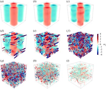


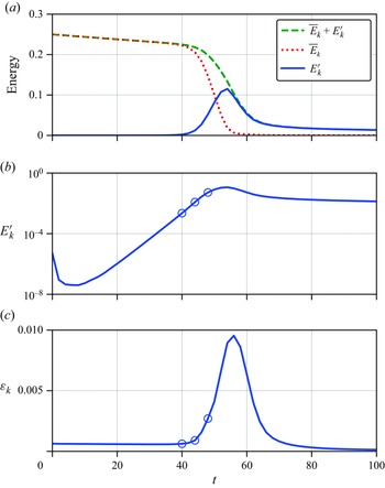


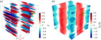


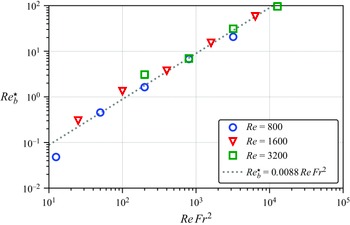


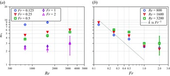


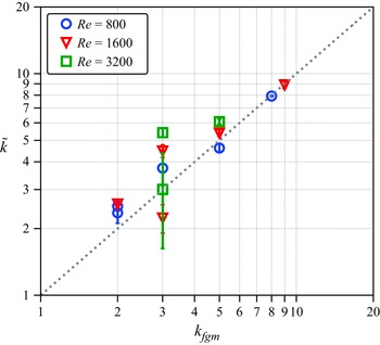


 Open access