


1. Introduction
Particles settling in a fluid medium under the influence of gravity has historically been a widely investigated research problem (Basset Reference Basset1888; Gatignol et al. Reference Gatignol1983; Maxey & Riley Reference Maxey and Riley1983; Boussinesq Reference Boussinesq1985; Magnaudet Reference Magnaudet1997). In the past few decades, researchers have devoted many efforts to understanding the effects of fluid density stratification on the settling dynamics of spherical particles, mainly motivated by geophysical applications (Doostmohammadi, Dabiri & Ardekani Reference Doostmohammadi, Dabiri and Ardekani2014; Ardekani, Doostmohammadi & Desai Reference Ardekani, Doostmohammadi and Desai2017; Magnaudet & Mercier Reference Magnaudet and Mercier2020). The most notable effect of density stratification on the motion of a spherical particle is drag enhancement. This observation has been confirmed by experiments (Lofquist & Purtell Reference Lofquist and Purtell1984; Srdić-Mitrović, Mohamed & Fernando Reference Srdić-Mitrović, Mohamed and Fernando1999; Yick et al. Reference Yick, Torres, Peacock and Stocker2009), theory (Mehaddi, Candelier & Mehlig Reference Mehaddi, Candelier and Mehlig2018) and computations (Torres et al. Reference Torres, Hanazaki, Ochoa, Castillo and Van Woert2000; Hanazaki, Konishi & Okamura Reference Hanazaki, Konishi and Okamura2009b). The immediate effect of this drag enhancement is to reduce the settling velocity of a sphere falling through a stratified fluid under the influence of gravity, an effect which should therefore be considered in large-scale transport models of environmental interest (Doostmohammadi et al. Reference Doostmohammadi, Dabiri and Ardekani2014).
Fluid stratification also modifies the flow structures around spherical particles in interesting ways. Depending on the Reynolds number of the moving particle,  $Re_p=U_{p}D/\nu$, and the Froude number of the flow,
  $Fr=U_{p}/ND$, a variety of jet structures can be observed (Hanazaki, Kashimoto & Okamura Reference Hanazaki, Kashimoto and Okamura2009a) behind a sphere with diameter
  $D$ moving vertically with a velocity
  $U_p$ in a stratified fluid with kinetic viscosity
  $\nu$ and Brunt–Väisälä frequency
  $N$. The formation of the jet influences a variety of phenomena in the oceans, such as the vertical movement of zooplankton and buoys used for ocean observation. Owing to the ubiquity of the density stratification due to salinity and/or temperature gradients in nature, e.g. in the atmosphere (Fernando et al. Reference Fernando, Lee, Anderson, Princevac, Pardyjak and Grossman-Clarke2001), lakes and oceans (MacIntyre, Alldredge & Gotschalk Reference MacIntyre, Alldredge and Gotschalk1995), it is obvious that studying how the density stratification influences the dynamics of settling/moving particles is crucial to understanding a plethora of natural phenomenon. For example, the atmospheric pollutants and pyroclastic particles (Cas & Wright Reference Cas and Wright1987) have sizes ranging from a few
  $\mathrm {\mu }{\textrm {m}}$ to a few mm with
  $Re_p$ in the range of
  $O(0\text {--}1000)$.
In oceans, the top layer,  $O \approx (1\text {--}1000)\,\textrm {m}$ deep, is associated with intense biological and ecological activities which are strongly influenced by the density stratification. The formation of algal blooms has been known to be a direct consequence of marine organisms’ interactions with density stratification (MacIntyre et al. Reference MacIntyre, Alldredge and Gotschalk1995). Stratification significantly alters the stability, interaction and nutrient uptake of organisms (Ardekani & Stocker Reference Ardekani and Stocker2010; Doostmohammadi, Stocker & Ardekani Reference Doostmohammadi, Stocker and Ardekani2012; More & Ardekani Reference More and Ardekani2020, Reference More and Ardekani2021). Stratification impacts carbon fluxes into the ocean by inhibiting the descent of marine snow particles (aggregates > 0.5 mm in diameter) (Alldredge & Gotschalk Reference Alldredge and Gotschalk1989). Furthermore, the vertical density stratification promotes accumulation of marine snow (Alldredge & Gotschalk Reference Alldredge and Gotschalk1989) and of phytoplankton (Cloern Reference Cloern1984). The
  $Re_p$ of these marine entities is
  $\approx O(0\text {--}100)$ depending on their sizes (Naganuma Reference Naganuma1996; Bochdansky, Clouse & Herndl Reference Bochdansky, Clouse and Herndl2016). The bio-convection in the oceans is an important step in the carbon cycle and is responsible for transferring approximately 300 million tons of carbon from the atmosphere to the oceans every year (Stone Reference Stone2010; Henson et al. Reference Henson, Sanders, Madsen, Morris, Le Moigne and Quartly2011). These observations make it imperative to investigate the role of density stratification on the dynamics of settling particles. However, the particles/organisms which are influenced by stratification are not exactly spherical. They come in a variety of shapes (Smayda & Morris Reference Smayda and Morris1980). The most common shapes that can be imagined are plate-like flat (Gibson, Atkinson & Gordon Reference Gibson, Atkinson and Gordon2007) or rod-like elongated (Bainbridge Reference Bainbridge1957). The extra degree of freedom introduced by the anisotropy of the particle shape leads to an interesting settling dynamics.
Even in a homogeneous fluid, the anisotropy of the settling particle shape leads to more convoluted phenomena like breaking of the flow axial symmetry, an oscillatory settling path and wake instability not observed for a spherical particle (Fernandes et al. Reference Fernandes, Risso, Ern and Magnaudet2007; Ern et al. Reference Ern, Risso, Fabre and Magnaudet2012). The influence of the body degrees of freedom on the wake dynamics along with the vorticity production at the body surface can explain the wake instabilities and their consequences for the body path (Namkoong, Yoo & Choi Reference Namkoong, Yoo and Choi2008; Ardekani et al. Reference Ardekani, Costa, Breugem and Brandt2016). Specifically, for oblate spheroids, four different states for the particle motion are observed for Galileo number,  $Ga=\sqrt {(|\rho _r-1|gD^3)/\nu ^2}$, between 50 to 250 (Chrust Reference Chrust2012; Ardekani et al. Reference Ardekani, Costa, Breugem and Brandt2016) for aspect ratio,
  $\mathcal {AR}=1/3$. Here,
  $g$ is the acceleration due to gravity,
  $\rho_r$ is the particle to fluid density ratio, and
  $D$ is the diameter of a sphere with the same volume as the spheroidal particle. The transition between the four states takes place at
  $Ga \approx 120$, 210 and 240 for
  $\rho _r=1.14$. On the other hand, the onset of secondary motions for prolate spheroids occurs at a considerably lower
  $Ga$ than for an oblate spheroid. The peculiar feature of settling prolate spheroids is that they attain a terminal rotational velocity about the axis parallel to the vertical direction in which it is falling freely for
  $Ga>70$ in the case of aspect ratio,
  $\mathcal {AR}=3$. This behaviour can be explained by the four thread-like quasi-axial vortices appearing in the wake of a prolate spheroid (Ardekani et al. Reference Ardekani, Costa, Breugem and Brandt2016). Recently, Roy et al. (Reference Roy, Hamati, Tierney, Koch and Voth2019) have presented theoretical and experimental evidence of an orientation transition of a fibre due to a gravitational torque that arises above a critical Reynolds number and showed the evolution of the oblique orientation toward the broad-side on orientation as
  $Re$ increased.
Although particle shape anisotropy leads to path and wake instabilities in the settling motion of particles in a homogeneous fluid, it does not change the steady-state settling orientations of the particles. The spheroidal particles have been observed to settle such that their long axis is always perpendicular to the settling direction (Feng, Hu & Joseph Reference Feng, Hu and Joseph1994; Fernandes et al. Reference Fernandes, Risso, Ern and Magnaudet2007, Reference Fernandes, Ern, Risso and Magnaudet2008; Ardekani et al. Reference Ardekani, Costa, Breugem and Brandt2016) for  $Re_p>0.1$. In addition, the particles reach a constant terminal velocity when falling freely in a homogeneous fluid. The terminal velocity depends on the
  $Ga$ and the aspect ratio of the particles.
The settling dynamics of spherical as well as non-spherical particles is significantly altered by the presence of fluid density stratification. The first notable departure from the settling in a homogeneous fluid is the absence of a terminal velocity. This is because stratification increases the drag experienced by the settling particles which therefore reduces their settling speeds. In addition, increasing buoyancy leads to the deceleration of the particle as it approaches the neutrally buoyant position and can cause oscillations in the particle velocity depending on the strength of stratification (Doostmohammadi et al. Reference Doostmohammadi, Dabiri and Ardekani2014).
Recently, researchers have started exploring the effects of stratification on the settling dynamics of anisotropically shaped particles in a stratified fluid. Most of the investigations are limited to disks. Experiments of a disk settling encountering a stratified two-layer fluid show that the disk reorients itself such that the long axis is perpendicular to the vertical direction while it moves through the transition layer between the two fluids (Mrokowska Reference Mrokowska2018, Reference Mrokowska2020a,Reference Mrokowskab). Further, a disk settling in a linearly stratified fluid has been observed to go through three regimes as it settles. First, there is a quasi-steady state with the disk long axis perpendicular to the vertical direction. Then, there is a change in the stability for the disk orientation when it changes its orientation from long axis normal to the vertical direction (broad-side on) to long axis parallel to the vertical axis (edge-wise). Finally, the disk settles edge-wise at its neutrally buoyant position (Mercier et al. Reference Mercier, Wang, Péméja, Ern and Ardekani2020). As concerns prolate spheroids, we can only mention the numerical study by Doostmohammadi & Ardekani (Reference Doostmohammadi and Ardekani2014), on the settling across a density interface. Hence, we are still far from completely understanding the settling and orientation dynamics of spheroidal shaped particles in a stratified fluid.
From a computational point of view, tracking an oblate and a prolate spheroid is similar but computationally, the simulations for prolate spheroids are more expensive. This is also true in the current numerical framework which will be discussed in the following sections. The scarcity of studies with prolate spheroids does not mean a lack of practical applications as elongated particles in a stratified fluid are routinely encountered in many industries involving suspensions of particles settling under gravity, pollutant transport in the atmosphere or water, fluidized beds and settling of marine snow or organisms in upper ocean layers. The most common shapes that can be imagined are plate-like flat (Gibson et al. Reference Gibson, Atkinson and Gordon2007) or rod-like elongated (Bainbridge Reference Bainbridge1957).
To gain some new understanding of the problem, we numerically simulate the free-falling motion of spheroidal particles, an oblate spheroid with an aspect ratio,  $\mathcal {AR}=1/3$ and a prolate spheroid with
  $\mathcal {AR}=2$, in a linearly stratified fluid for different
  $Ga$ and
  $Fr$ values. The aim of this effort is to investigate the possible mechanism which leads to the orientational instability of a freely falling spheroidal object in a linearly stratified fluid.
2. Governing equations
We present the governing equations and the solution methodology implemented to solve them in this section. We solve the Navier–Stokes equations and the continuity equation in terms of the perturbation velocity field and calculate the perturbation flow field  $\boldsymbol {u'}=\boldsymbol {u}-\boldsymbol {U}_p$, where
  $\boldsymbol {u}$ is the fluid velocity field and
  $\boldsymbol {U}_p$ is the instantaneous particle velocity. We assume the fluid to be Newtonian and incompressible and assume the Boussinesq approximation for the density to be valid which means we can ignore density differences everywhere except in the gravitational body force term. These assumptions result in the following equations, written in the reference frame translating with the particle velocity
  $\boldsymbol {U}_p$:
 \begin{gather} \rho_f\left( \frac{\partial\boldsymbol{u'}}{\partial{t}} + \left( \boldsymbol{u'}-\boldsymbol{U}_p \right) \boldsymbol{\cdot} \boldsymbol{\nabla}{\boldsymbol{u'}} \right) ={-}\boldsymbol{\nabla}{p} + \mu{\boldsymbol{\nabla}}^{2}\boldsymbol{u'}+\rho_f \left( {\boldsymbol{g}}+\boldsymbol{f} \right), \end{gather}
 \begin{gather} \boldsymbol{\nabla} \boldsymbol{\cdot} \boldsymbol{u'} = 0, \end{gather}
where  $\rho _f$ is the density field,
  $\boldsymbol {U}_p$ is the instantaneous particle translational velocity,
  $p$ is the pressure,
  $\mu$ is the fluid dynamic viscosity,
  $\boldsymbol {g}$ is the acceleration due to gravity. The additional term
  $\boldsymbol {f}$ on the right-hand side of (2.1) accounts for the presence of particle, modelled with the immersed boundary method (IBM). This IBM force is active in the immediate vicinity of a particle to impose the no-slip and no-penetration boundary conditions indirectly. In other words, the force distribution
  $\boldsymbol {f}$ ensures that the fluid velocity at the surface is equal to the particle surface velocity (
 $\boldsymbol {U}_p + \boldsymbol {\omega }_p \times \boldsymbol {r}$).
The particle motion is solution of the following Newton–Euler Lagrangian equation of particle motion:
 \begin{gather} {\rho}_p {V_{p}} \frac{\text{d}\boldsymbol{U}_p}{\text{d}t} = \oint_{\partial{V}_p} \boldsymbol{\tau} \boldsymbol{\cdot} \boldsymbol{n} \, \text{d}A, \end{gather}
 \begin{gather} \frac{ \text{d} \left( \boldsymbol{I}_p \boldsymbol{\omega}_p \right) }{\text{d}t} = \oint_{\partial{V}_p} {\boldsymbol{r} \times \left( \boldsymbol{\tau} \boldsymbol{\cdot} \boldsymbol{n} \right) \, \text{d}A}, \end{gather}
here,  $\boldsymbol {U}_p$ and
  $\boldsymbol {\omega }_p$ are the particle translational and angular velocities;
  $\rho _p$,
  $V_p$ and
  $\boldsymbol {I}_p$ represent the particle density, particle volume and the particle moment of inertia matrix;
  $\boldsymbol {n}$ is the unit normal vector pointing outwards on the particle surface, while
  $\boldsymbol {r}$ is the position vector from the particle's centre;
  $\boldsymbol {\tau } = -p\boldsymbol {I}+\mu ( \boldsymbol {\nabla }\boldsymbol {u} + \boldsymbol {\nabla }\boldsymbol {u}^{\textrm {T}} )$ is the stress tensor and its integration on the particle surface accounts for the fluid–particle interaction.
Accounting for the inertia and buoyancy forces of the fictitious fluid phase inside the particle volume and using IBM, (2.3) and (2.4) are rewritten as follows:
 \begin{gather} \rho_p V_p \frac{ \mathrm{d} \boldsymbol{U}_{p}}{\mathrm{d} t} \, \approx \, -\rho_0 \sum_{l=1}^{N_L} \boldsymbol{F}_l \Delta V_l + \rho_0 \frac{ \mathrm{d}}{\mathrm{d} t} \left( \int_{V_p} \boldsymbol{u}\,\mathrm{d} V \right) - \int_{V_p} \rho_f \boldsymbol{g}\,\mathrm{d} V + \rho_p V_p \boldsymbol{g} , \end{gather}
 \begin{gather} \frac{ \mathrm{d} \left( \boldsymbol{I}_p \, \pmb{\omega}_{p} \right) }{\mathrm{d} t} \, \approx \, -\rho_0 \sum_{l=1}^{N_L} \boldsymbol{r}_l \times \boldsymbol{F}_l \Delta V_l + \rho_0 \frac{ \mathrm{d}}{\mathrm{d} t} \left( \int_{V_p} \boldsymbol{r} \times \boldsymbol{u} \mathrm{d} V \right) - \int_{V_p} \boldsymbol{r} \times \rho_f \boldsymbol{g}\, \mathrm{d} V , \end{gather}
where the first two terms on the right-hand side of the equations denote the hydrodynamic force and torque  $F_h$ and
  $T_h$, respectively. The third term and the fourth term together in (2.5) indicate the buoyancy force
  $F_b$ while the third term in (2.6) indicates the buoyancy torque
  $T_b$. More details on the numerical model can be found in Ardekani et al. (Reference Ardekani, Abouali, Picano and Brandt2018a) and Majlesara et al. (Reference Majlesara, Abouali, Kamali, Ardekani and Brandt2020).
The vertical variation in the fluid density can either be due to the vertical variation in the fluid temperature or salinity or both. For this study we consider the density stratification to arise from the fluid temperature variation. Thus, the particle sediments in a linearly density stratified fluid with the initial vertical density stratification given by  $\bar {\rho }(z) = \rho _0 - \gamma {z}$. Here,
  $\rho _0$ is the reference density,
  $\gamma$ is the vertical density gradient and
  $z$ is the vertical coordinate. The fluid density increases linearly in the downward
  $z$ direction (gravity direction). The density variation across thermocline occurs due to the vertical variation in the temperature, since
  $\rho = \rho _0 ( 1 - \beta ( T - T_0) )$, where
  $\beta$ is the coefficient of thermal expansion,
  $T$ is the temperature field and
  $T_0$ is the reference temperature corresponding to the reference density,
  $\rho _0$. Thus, the initial temperature of the background fluid is given by
  $\bar {T}(z) = T_0 + (\gamma /\beta \rho _0)z$. The energy equation for an incompressible fluid flow in the frame of reference moving with the particle can be simplified to,
 \begin{equation} \frac{\partial{T}}{\partial{t}} + \left( \boldsymbol{u}'-\boldsymbol{U}_p \right) \boldsymbol{\cdot} \boldsymbol{\nabla}{T} = \boldsymbol{\nabla} \boldsymbol{\cdot} \left( \alpha \boldsymbol{\nabla} T \right). \end{equation}
Here,  $\alpha$ is the thermal diffusivity. We split the temperature field in the linear component and the perturbation (
 $T^{'}$) as
  $T = \bar {T}(z) + T^{'}$. We solve for the temperature perturbation,
  $T^{'}$, and add it to the linear component to get the temperature field at any instance of time. (2.7) can be rewritten in term of the temperature perturbation field,
  $T^{'}$ as follows:
 \begin{equation} \frac{\partial{T^{'}}}{\partial{t}} + \left( \boldsymbol{u}'-\boldsymbol{U}_p \right) \boldsymbol{\cdot} \boldsymbol{\nabla}({\bar{T}(z) + T^{'}}) = \boldsymbol{\nabla} \boldsymbol{\cdot} ( \alpha \boldsymbol{\nabla} T^{'} ). \end{equation}
We set  $\alpha = 0$ for the particle (Doostmohammadi et al. Reference Doostmohammadi, Dabiri and Ardekani2014) and
  $\alpha =\nu /Pr$ for the fluid phase;
  $\nu$ is the fluid kinematic viscosity and
  $Pr$ is the Prandtl number. This is equivalent to the insulating/impermeable/no-flux boundary condition on the surface of the particle (Hanazaki et al. Reference Hanazaki, Konishi and Okamura2009b; Doostmohammadi et al. Reference Doostmohammadi, Dabiri and Ardekani2014) which is also true if the stratifying agent is salt or having an adiabatic particle. We also investigate the effects of relaxing the no-flux boundary condition on the particle surface by varying
  $\alpha$ for the particle by changing the particle heat conductivity,
  $k$, in § 3.3.
2.1. Dimensionless parameters and simulation conditions
Re-writing the equations in the non-dimensional form results in the following equations:
 \begin{gather} \frac{\partial \boldsymbol{u}}{\partial{t}} + \left( \left( \boldsymbol{u}-\boldsymbol{U}_p \right) \boldsymbol{\cdot} \boldsymbol{\nabla} \right) \boldsymbol{u} ={-}\boldsymbol{\nabla}{P} + \frac{1}{Re}{\boldsymbol{\nabla}}^{2}\boldsymbol{u}+ \frac{Ri}{Re} T + \boldsymbol{f}, \end{gather}
 \begin{gather} \frac{\partial T}{\partial{t}} + \left( \boldsymbol{u}-\boldsymbol{U}_p \right) \boldsymbol{\cdot} \boldsymbol{\nabla}{T} + \boldsymbol{u} \boldsymbol{\cdot} \hat{e}_g = \frac{1}{\rho^* C^*_p} \boldsymbol{\nabla} \boldsymbol{\cdot} \left( \frac{k^*}{Re Pr} \boldsymbol{\nabla} T \right), \end{gather}
 \begin{gather} \boldsymbol{\nabla} \boldsymbol{\cdot} \boldsymbol{u} = 0, \end{gather}
where,  $\boldsymbol {u}$,
  $T$ and
  $P$ now denote dimensionless perturbations in velocity, temperature and pressure field. Temperature is normalized with the temperature difference of
  $1$ equivalent particle diameter in the gravity direction;
  $\rho ^*$,
  $C^*_p$ and
  $k^*$ indicate particle density, heat capacity and heat conductivity ratio (
 $\rho _r$,
  ${C_p}_r$ and
  $k_r$) inside the particles and are equal to
  $1$ in the fluid region. We investigate the sedimentation of spheroidal particles in a quiescent but linearly density-stratified fluid with finite inertia. The details on the numerical algorithm to solve the governing equations and validations of the numerical tool are provided elsewhere (Ardekani et al. Reference Ardekani, Costa, Breugem and Brandt2016, Reference Ardekani, Asmar, Picano and Brandt2018b; Ardekani Reference Ardekani2019) and hence not discussed here.
The non-dimensional parameters defining the problem are described below:
(i) The Galileo number,
 $Ga={U} D/\nu$, with the reference velocity ${U}$ defined as ${U}=\sqrt {D|\rho _r-1|g}$; $D$ is the length scale corresponding to the particle size, set as the diameter of a sphere with the same volume as that of the spheroidal particle ($D=(b^2a)^{(1/3)}$); $a$ and $b$ denote the polar and the equatorial radius of the spheroidal particle; $Ga$ quantifies the relative importance of gravitational and viscous forces.
(ii) The particle Reynolds number,
$Re_p= {U_p} D/\nu$, which quantifies the relative importance of the inertial and the viscous forces. Here, $U_p$ is the instantaneous particle velocity so this is a non-dimensional measure of the particle settling speed.(iii) The Richardson number,
$Ri=\gamma g D^3 / ({U} \rho _0 \nu ) = D^3N^2/ ({U} \nu )$, which quantifies the relative importance of buoyancy and the viscous time scales; $N= {(\gamma {g}/\rho _{0})}^{1/2}$ is the Brunt–Väisälä frequency. It is the natural frequency of oscillation of a vertically displaced fluid parcel in a stratified fluid.(iv) The Prandtl number,
$Pr = C_p \mu / k$, defined as the ratio of momentum diffusivity to thermal diffusivity inside the fluid region.(v) The particle density ratio, indicating the ratio between the particle density and the reference density of the fluid;
$\rho _r = \rho _p/\rho _0$.(vi) The particle heat conductivity ratio,
$k_r = k_p/k_f$, with subscripts $p$ and $f$ denoting the particle phase and the fluid phase.(vii) The particle heat capacity ratio,
${C_p}_r = {C_p}_p / {C_p}_f$.(viii) The particle aspect ratio,
$\mathcal {AR}=a/b$.


Finally, the characteristic time scale,  $\tau$, used to make
  $t$ dimensionless is chosen to be
  $\tau =D/{U}$. In (2.9) and 2.10,
  $Re$ is the Reynolds number which has the same definition as the Galileo number,
  $Ga$. Please note that we use
  $Re_p$ to denote the instantaneous Reynolds number of the particle which changes with time and particle location;
  $Re_p$ is used later for drag calculations.
We simulate the sedimenting motion of a spheroidal shaped particle in a linearly density stratified fluid using a three-dimensional rectangular domain of size  $20D \times 20D \times 80D$ (
 $10D \times 10D \times 40D$) for an oblate (prolate) spheroid with grid size equal to
  $D/32$ (
 $D/48$), resulting in
  $\approx O(10^9)$ (
 $\approx O(5 \times 10^8)$) grid points. We use periodic boundary conditions for the velocity field and the temperature perturbations on all the sides of the domain. We consider an oblate particle with aspect ratio,
  $\mathcal {AR} = a/b = 1/3$ (figure 1a) and a prolate particle with
  $\mathcal {AR} = a/b = 2$ (figure 1b). Since we solve the flow field in the frame translating with the particle, the particle stays at its initial position, i.e. ([
 $10D, 10D, 20D$] for an oblate spheroid and [
 $5D, 5D, 10D$] for a prolate spheroid). The domain sizes chosen ensure that there is no significant interaction between the particles and its wake for the entire parameter range explored in this study as shown in the Appendix.
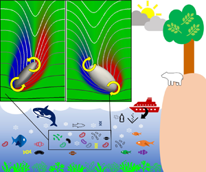
Schematic of the settling spheroidal objects in a linearly density-stratified fluid. (a) Oblate spheroid ( $\mathcal {AR}<1$) and (b) prolate spheroid (
 $\mathcal {AR}>1$). Here,
  $a$ and
  $b$ are the semi-major and the semi-minor axes. The aspect ratio
  $\mathcal {AR}$ is given by
  $a/b$. For spherical particles
  $\mathcal {AR}=1$. The orientation of the particle is quantified in terms of the polar angle
  $\theta$ and the azimuthal angle
  $\phi$ for a vector directed along the major axis of the spheroids. The coordinate system used is shown at the top of the figures.

Depending on the hydrodynamic torque it experiences, the particle can rotate freely. The orientation of the spheroid is measured in terms of the polar angle  $\theta$, which is the angle made by the major axis of the spheroid with the
  $z$-axis as shown in figure 1. In the atmosphere, the typical value of
  $N$ is
  $10^{-2}\,\textrm {s}^{-1}$ while in the ocean
  $N$ is around
  $10^{-4}-0.3 \,\textrm {s}^{-1}$ depending on the strength of density stratification (Geyer, Scully & Ralston Reference Geyer, Scully and Ralston2008; Wüst et al. Reference Wüst, Bittner, Yee, Mlynczak and Russell III2017). We perform simulations for
  $Ga = 80-250$, while we vary
  $Ri$ between 0 and 10 (or
  $N \approx 0.04 - 0.2\,\textrm {s}^{-1}$), which are consistent with the typical value of
  $N$ mentioned above;
  $Ri=0$ represents a particle settling in a homogeneous fluid with a constant density. We fix the density ratio,
  $\rho _r=1.14$ in all the cases. The temperature inside the particle is set similar to the surrounding fluid initially, resulting in a domain with zero temperature fluctuations at the start of the simulations.
We use  $Pr=0.7$ for all the simulation cases in this study except in § 3.4 where we investigate the effect of changing fluid
  $Pr$;
$Pr$;  $Pr=0.7$ corresponds to temperature stratified atmosphere, while
  $Pr=7$ and
  $Pr=700$ correspond to temperature-stratified water and salt stratified water, respectively. In a stratified fluid, a density boundary layer is present in addition to the velocity boundary layer near the particle surface. The thickness of this density boundary layer scales as
  $\approx O(D/\sqrt {RePr})$. For accurate resolution of the flow within this boundary layer, it is necessary to have at least a few grid points in it. This imposes limitations on the maximum mesh size that can be used for the simulations. Owing to large size of the domain, using such a fine grid becomes computationally expensive. Hence, we use a smaller value for the
  $Pr$ which enables us to resolve the fluid flow as well as the density field in both the boundary layer and the outside. We show in § 3.4 (in agreement with previous studies Doostmohammadi et al. Reference Doostmohammadi, Dabiri and Ardekani2014) that, changing the value of
  $Pr$ merely changes the magnitudes of the velocities of the objects moving in a stratified fluid conserving the overall qualitative trends and behaviours. Finally, it should be noted that though we use the
  $N$ and
  $Pr$ values corresponding to a temperature-stratified atmosphere and water, the density ratio chosen, i.e.
  $\rho _r=1.14$ is representative of particles settling in an ocean rather than in a stratified air. A realistic
  $\rho _r$ for atmospheric particles would be
  $\approx O(10^3)$ resulting in large inertial effects and effectively subverting any governing influence of density stratification. Hence, the simulations presented here are not intended to mimic any atmospheric phenomenon but are intended to provide crucial insights in understanding the sedimentation of individual particles/organisms through oceanic thermoclines. The motivation for the chosen value of
  $Pr$ is computational convenience. Table 1 summarizes the values of all the relevant parameters investigated.
Values of relevant parameters investigated in this study.

3. Results and discussion
The following subsections present the simulation results for settling spheroids in a stratified fluid. We present the settling velocities and orientations of the spheroids for the range of  $Ga$ and
  $Ri$ investigated. We first present and discuss the results for an oblate spheroid followed by the results for the prolate spheroid. We compare the data from the stratified fluid case with the data from the homogeneous fluid case to better understand the results. We use ‘broad-side on’ to indicate an orientation of the spheroidal particles such that their broader side is horizontal, i.e.
  $\theta =0^{\circ }$ for an oblate spheroid and
  $\theta = 90^{\circ }$ for a prolate spheroid. On the other hand, ‘edge-wise’ indicates the orientation of the particles in which their broader side is perpendicular to the horizontal direction, i.e.
  $\theta = 90^{\circ }$ for an oblate spheroid and
  $\theta = 0^{\circ }$ for a prolate spheroid.
3.1. Settling dynamics of an oblate spheroid in a stratified fluid
3.1.1. Fluid stratification slows down and reorients a settling oblate spheroid
This subsection presents the simulation results for an oblate spheroid with  $\mathcal {AR}=1/3$ settling in a stratified fluid. The oblate spheroid starts from rest in an initially quiescent fluid. The spheroid velocity then evolves depending on the hydrodynamic and buoyancy forces acting on it as the flow evolves. We initialize the orientation of the oblate spheroid such that
  $\theta = 90^{\circ }$ or in edge-wise orientation. In a homogeneous fluid, the oblate spheroid accelerates and attains a terminal velocity after the initial transients (which are due to the oscillations in the spheroid orientation) as shown in figure 2(a). In addition, as the oblate spheroid accelerates, it topples from its initial edge-wise to a broad-side on orientation. However, due to its inertia and periodic shading of hairpin-like vortex structures from alternate edges (Ardekani et al. Reference Ardekani, Costa, Breugem and Brandt2016), it oscillates around the broad-side on (
 $\theta =0^{\circ }$) orientation. So, for
  $Ga=210$, an oblate spheroid settles in an oscillatory orientation about
  $\theta =0^{\circ }$, as shown in figure 2(b) for
  $Ri=0$. The oscillations are not present at lower
  $Ga$ (
 $<120$) (Ardekani et al. Reference Ardekani, Costa, Breugem and Brandt2016).
Settling dynamics of an oblate spheroid ( $\mathcal {AR}=1/3$) with
  $Ga=210$ in a homogeneous fluid (
 $Ri=0$) and a stratified fluid with different
  $Ri$ values: (a) settling velocity evolution, (b) spheroid orientation evolution vs time. The insets in both the figures show the initial oscillations with decreasing amplitudes in the velocity and orientation of the spheroid. The oblate spheroid attains a steady-state terminal velocity and oscillates about the broad-side on orientation in a homogeneous fluid after the initial transients. Stratification leads to a reduction in the spheroid velocity and a continuous deceleration of the spheroid velocity until it stops. The magnitude of the deceleration increases with stratification. In addition, the steady-state orientation of the oblate spheroid changes from broad-side on (i.e.
  $\theta = 0^{\circ }$) in a homogeneous fluid to edge-wise (i.e.
  $\theta \approx 90^{\circ }$) in a stratified fluid. The transition in the orientation starts once the magnitude of the dimensionless spheroid velocity drops below a particular threshold. Here,
  $|U_p/U| < 0.15$. The onset of transition in the spheroid orientation is denoted by dotted horizontal line in (a) and yellow stars in (b).

Introducing density stratification in the fluid significantly changes the settling dynamics of an oblate spheroid. This is shown in figure 2 for  $Ga=210$ and various
  $Ri$ as well as in figure 3 for
  $Ri=3$ and various
  $Ga$ values. As the oblate spheroid sediments in a stratified fluid, it moves from a region with lighter fluid into a region with heavier fluid. As a result, it experiences an increasing buoyancy force which essentially opposes its settling motion. Hence, the particle cannot attain a steady-state terminal velocity. This phenomenon is clearly depicted in figures 2(a) and 3(a) where the particle velocity decreases continuously after the initial transients. The suppression of the fluid flow due to the tendency of the displaced iso-density difference surfaces (isopycnals) to return to their original locations is another reason for the reduction in the particle velocity (see the detailed discussion in § 3.1.3 and figure 8).
Settling dynamics of an oblate spheroid in a stratified fluid and  $Ri=3$ with different
  $Ga$ values: (a) settling velocity, (b) spheroid orientation evolution vs time. The insets show the initial oscillations with decreasing amplitude. The oblate spheroid attains a steady-state terminal velocity and orientation (broad-side on,
  $\theta = 0 ^{\circ }$) in a homogeneous fluid. Stratification leads to a reduction in the spheroid velocity and a continuous deceleration of the spheroid velocity until it stops. The magnitude of the deceleration decreases with increasing the particle inertia. In addition, the steady-state orientation of the oblate spheroid changes from broad-side on (i.e.
  $\theta = 0^{\circ }$) in a homogeneous fluid to broad-side perpendicular (i.e.
  $\theta \approx 90^{\circ }$) in a stratified fluid. The transition in the orientation starts once the magnitude of the dimensionless spheroid velocity drops below a threshold. Here,
  $|U_p/U| < 0.15$. The onset of transition in the spheroid orientation is denoted by the dotted horizontal line in (a) and the yellow stars in (b).

An increase in the stratification strength of the background fluid increases the magnitude of the particle deceleration. This is expected as the magnitude of the buoyancy force experienced by the particle increases with the fluid stratification. As a result, the particle stops at earlier times for increasing  $Ri$ values as shown in figure 2(a). Another consequence of this increased opposition to the settling motion is the reduction in its peak velocity when increasing the stratification as shown in figure 2(a). In addition, as the
  $Ga$ of the particle increases for a fixed
  $Ri$, the magnitude of deceleration decreases as shown in figure 3(a). This is because of the increase in the inertia of the particle with
  $Ga$.
$Ga$.
A closer comparison between the time histories of the velocity and orientation reveals that, the onset of reorientation of the oblate spheroid is connected to the reduction of the settling velocity below a certain threshold. From the simulation data, we observe that, the reorientation starts once the magnitude of the dimensionless velocity of the particle falls below  $\approx 0.15$. This is indicated by a horizontal dashed line in the velocity evolution plots and a star in the spheroid orientation evolution plots (see figures 2 and 3). This observation is consistent with the experimental and numerical study on the orientation of a settling disk in a stratified fluid by Mercier et al. (Reference Mercier, Wang, Péméja, Ern and Ardekani2020). Since stratification leads to a reduction in the particle velocity, an oblate spheroid eventually settles in an edge-wise orientation. This is because after a long enough time, the particle velocity goes below the threshold velocity for the onset of reorientation in a stratified fluid.
We quantify the effects of fluid density stratification on the peak velocity of the particles in figure 4(a). We define the peak velocity as the maximum velocity achieved by the particles as it settles. We observe that the peak velocity decreases monotonically with the fluid stratification strength and increases with increasing  $Ga$. Also, the relative decrease in the peak velocity for the lowest to the highest stratification strengths explored reduces with the Reynolds number. For
  $Ga=80$ it decreases by
  $\approx 20\,\%$ while for
  $Ga=250$ it decreases by
  $\approx 6\,\%$. This is due the increase in the strength of the inertial effects as compared with the stratification effects with increasing
  $Ga$ at fixed
  $Ri$. As concluded from figures 2(a) and 3(a), increasing the stratification strength or reducing the inertia of the particle moves the onset of the reorientation instability to an earlier time. Figure 4(b) shows the effect of changing particle
  $Ga$ and
  $Ri$ on the time for the onset of reorientation instability. We observe that, the time (
 $(t/\tau )_{threshold}$) at which particle velocity falls below the threshold velocity for the onset of reorientation instability decreases as
  $O(Ri^{-1})$.
Effect of inertia and stratification strength on (a) the peak velocity,  $(U_p(t)/U)_{peak}$, of a settling oblate spheroid with
  $\mathcal {AR}=1/3$. The peak velocity attained by the particle decreases stratification and increases with increase in particle inertia, and (b) the time (
 $(t/\tau )_{threshold}$) at which
  $|U_p(t)/U| < 0.15$. The dashed line in (a) is a guide to the eye. The dotted line in (b) is the
  $(t/\tau )_{threshold} = A*Ri^{-1}$ fit with A = 153.7, 310.5, 384.8 and 455.5 for
  $Ga=80$,
  $170$,
  $210$ and
  $250$, respectively.

3.1.2. Disappearance of oscillatory paths of settling oblate spheroid
An oblate spheroid settling in a homogeneous fluid exhibits four distinct trajectories depending on its  $Ga$ (Ardekani et al. Reference Ardekani, Costa, Breugem and Brandt2016). An oblate spheroid with
  $\mathcal {AR} = 1/3$ falls in a straight line with an axisymmetric wake for
  $Ga \lessapprox 120$. Increasing
  $Ga$ further eliminates the axisymmetry and introduces oscillations in the settling path. The path is fully vertical with periodic oscillations for
  $Ga \lessapprox 210$. A weakly oblique oscillatory state motion is observed in the range
  $210 \lessapprox Ga \lessapprox 240$ whereas for
  $Ga \gtrapprox 240$ the particle path becomes chaotic with patterns of quasi-periodicity. These four states of motion can be explained by the wake instabilities behind a settling oblate spheroid (Ardekani et al. Reference Ardekani, Costa, Breugem and Brandt2016) similar to the wake instabilities behind a settling disk (Magnaudet & Mougin Reference Magnaudet and Mougin2007; Yang & Prosperetti Reference Yang and Prosperetti2007; Ern et al. Reference Ern, Risso, Fabre and Magnaudet2012).
Stratification significantly alters the settling paths of an oblate spheroid. In particular, it completely annihilates the oscillatory trajectories experienced by a settling oblate spheroid at  $Ga \gtrapprox 120$ as shown in figures 5(b), 5(c) and 5(d). Comparing the trajectories at different non-zero
  $Ri$ for various
  $Ga$ in figure 5 shows that an oblate spheroid experiences a qualitatively similar trajectory (after the initial transients which will be absent if we initialize the oblate spheroid with the broad-side on orientation) irrespective of its
  $Ga$ and
  $Ri$. The settling path can be divided into three regions.
Trajectories of an oblate spheroid with  $\mathcal {AR}=1/3$ in a homogeneous and a stratified fluid for different
  $Ga$ and
  $Ri$; (a)
  $Ga=80$, (b)
  $Ga=170$, (c)
  $Ga=210$, (d)
  $Ga=250$ and (e) a schematic summarizing the settling velocity, particle trajectory and the orientation in the three zones identified in the settling motion of an oblate spheroid in a stratified fluid. Left vertical axis and bottom horizontal axis indicate spheroid position (solid line is the settling trajectory). Right vertical axis and top horizontal axis are for particle settling velocity vs time (dashed line is the settling velocity).

Initially, as the spheroid accelerates from rest, it sediments approximately in a straight line until its velocity approaches the threshold for the reorientation onset. We call this region  $I$. In region
  $II$, the oblate spheroid starts reorienting due to the onset of the reorientation instability. This induces a non-zero horizontal velocity component in the settling of an oblate spheroid. As a result, the particle moves in the horizontal direction, breaking the straight line motion and getting deflected in the transverse direction. This region can also be identified in the settling velocity of the oblate spheroid. The settling velocity attains a temporary plateau after it falls below the threshold for reorientation. During this time, the oblate spheroid experiences reorientation from broad-side on to edge-wise and gets deflected in the horizontal direction. This horizontal deflection has previously been observed for disks (Mrokowska Reference Mrokowska2018; Mercier et al. Reference Mercier, Wang, Péméja, Ern and Ardekani2020; Mrokowska Reference Mrokowska2020a). This region ends when the reorientation is over and the settling velocity increases momentarily as can be seen in figure 2(a). Finally, in region
  $III$, as the particle comes close to its neutrally buoyant position, its velocity quickly decelerates and stops which is indicated by the reversal of the horizontal trajectory at the end of the settling path in figure 5. These settling trajectories and regions are similar to those observed for a disk in a stratified fluid (Mercier et al. Reference Mercier, Wang, Péméja, Ern and Ardekani2020). However, we do not observe any change in the orientation of an oblate spheroid from edge-wise at the end of region
  $III$ as observed for a disk (Mercier et al. Reference Mercier, Wang, Péméja, Ern and Ardekani2020). This is most likely because of the ideal conditions in simulations as opposed to experiments. Figure 5(e) summarizes the three regions of the settling path of an oblate spheroid in a stratified fluid along with their onset conditions on the settling velocity evolution plot.
3.1.3. What causes deceleration and reorientation of an oblate spheroid in a stratified fluid?
In the case of disk-like bodies settling in a homogeneous fluid, the path instabilities as described in the last subsection can be explained by the wake instabilities (Magnaudet & Mougin Reference Magnaudet and Mougin2007; Yang & Prosperetti Reference Yang and Prosperetti2007; Ern et al. Reference Ern, Risso, Fabre and Magnaudet2012). Therefore, analysing the wake vortices can provide insight into the mechanisms leading to a particular type of motion in either a homogeneous or a stratified fluid. For an oblate spheroid settling in a homogeneous fluid, a single toroidal vortex attached to the particle is initially formed. This is similar to a spherical particle moving with a steady velocity in a homogeneous fluid. As time passes, instabilities develop and the particle starts rotating around one of its major axes, normal to the direction of gravity, as shown in figure 2(b). As the angle of the oblate spheroid with respect to the horizontal axis increases, a part of this toroidal vortex detaches from the particle in a hairpin-like structure (Ardekani et al. Reference Ardekani, Costa, Breugem and Brandt2016). Vortices are associated with low pressure regions rather than the ambient. So, as a result of the detachment of the toroidal vortex, the oblate spheroid experiences a torque due to the formation of this low pressure region behind it which directly opposes the rotation of the particle in the other direction. Owing to inertia, the particle then rotates in the other direction. New hairpin vortices keep detaching from the oblate spheroid alternatively from either side as it settles, leading to periodic changes in the orientation and oscillatory paths (Ardekani et al. Reference Ardekani, Costa, Breugem and Brandt2016).
The situation is completely different in the case of an oblate spheroid settling in a stratified fluid. This is due to the fact that stratification suppresses the vertical motion of the fluid (Ardekani & Stocker Reference Ardekani and Stocker2010; Doostmohammadi et al. Reference Doostmohammadi, Dabiri and Ardekani2014; More & Balasubramanian Reference More and Balasubramanian2018 as shown by the isopycnals in figure 8) and prevents the particle from attaining any steady-state speed. As a result, there is no mechanism which can lead to periodic vortex shedding as described above. Conversely, we observe two toroidal vortices, one attached to the particle and one detached from the particle, as shown in figure 6. Once the particle velocity falls below the threshold velocity for reorientation, the detached vortex is asymmetric and does not oscillate from one side to the other unlike the case of an oblate spheroid sedimenting in a homogeneous fluid. As a result, there is a consistent low pressure region behind the oblate spheroid which predominantly remains on one side. This results in a torque on the particle which reorients it until it reaches its neutrally buoyant position. Eventually, as the oblate stops, the torque acting on it also vanishes and it stops in the edge-wise orientation.
Dimensionless iso-surfaces of Q-criterion (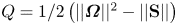 $Q = 1/2 \left( ||\boldsymbol{\varOmega}||^2 - ||\mathbf{S}|| \right)$ where
  $\mathbf{S}=1/2\left( \nabla \mathbf{u} + \nabla \mathbf{u}^{\rm T} \right)$ is the rate of strain tensor and
  $\boldsymbol{\varOmega}=1/2\left( \nabla \mathbf{u} - \nabla \mathbf{u}^{\rm T} \right)$ is the vorticity tensor) equal to
  $5 \times 10^{-4}$ for an oblate spheroid with
  $\mathcal {AR}=1/3$,
  $Ga=80$ and
  $Ri=5$ at equal time intervals of
  $t/ \tau =10.74$ starting from
  $t/ \tau = 18.78$. These contours show the evolution of vortices. The vortical structures identified by the positive Q-criterion are associated with a lower pressure region behind the particle.

To make this point clear, we measure the forces and torques acting on the spheroid. As shown in the methodology section, the force (torque) acting on the spheroid can be split into two components ((2.5) and (2.6)): (i)  $\boldsymbol {F}_h$ (
 $\boldsymbol {T}_h$) , arising from the hydrodynamic stresses acting on the particle surface, denoted as the hydrodynamic force (hydrodynamic torque), and (ii)
  $\boldsymbol {F}_{b}$ (
 $\boldsymbol {T}_b$), arising from the buoyancy or the density disturbance at the particle surface, denoted as the buoyancy force (buoyancy torque). The reason behind the deceleration of the spheroid and its reorientation becomes clear by looking at the
  $z$-component of the forces and the
  $x$-component of the torques acting on the spheroid shown for an oblate spheroid with
  $\mathcal {AR}=1/3$,
  $Ga=80$ and
  $Ri=5$ in figure 7.
(a) Forces acting on the oblate spheroid with  $Ga=80$ as it settles in a stratified fluid with varying
  $Ri$ shown with different colours. The total force (solid line) can be split into two components, the hydrodynamic component (dashed line) and the buoyancy component (dotted line). (b) The
  $x$-component of the torque acting on the oblate spheroid with
  $Ga=80$ as it sediments in a stratified fluid with
  $Ri=5$ along with the
  $x$-component of the angular velocity. The net torque (solid line) is split into two components, the hydrodynamic torque (dotted line) which tries to orient it in a broad-side on orientation (hence stabilizing) and the buoyancy component (dashed-dotted line) which is destabilizing and tries to reorient it in a edge-wise orientation. The reorientation starts once the magnitude of hydrodynamic torque falls below the buoyancy torque which happens when the particle velocity falls below the threshold for reorientation as discussed in § 3.1.1.

Initially, the density difference between the particle and the local surrounding fluid results in a high buoyancy force (high  $F_{b,z}$) on the spheroid resulting in its acceleration (negative
  $F_z$ at the initial
  $t/\tau$ in figure 7a). As the spheroid accelerates, the magnitude of the hydrodynamic drag increases (
 $F_{h,z}$ increases) and the buoyancy force decreases in a region with increasing fluid density. Hence, the spheroid accelerates until the magnitude of the hydrodynamic drag becomes larger than the buoyancy force (
 $F_{h,z} > F_{b,z}$), at which point it attains the maximum velocity. The buoyancy force is unable to overcome this increasing hydrodynamic drag which leads to the deceleration of the spheroid (
 $F_z > 0$ meaning the net force acting on the spheroid is in the opposite direction to its motion). Eventually, as the particle reaches its neutrally buoyant position, it stops as there is no net force acting on it. In a homogeneous fluid, i.e.
  $Ri=0$, the buoyancy force acting on the particle is constant,
  $F_{b,z} = (\rho _p-\rho _f)V_pg$ and the hydrodynamic drag balances the buoyancy force at steady state, resulting in a constant terminal velocity.
To understand the reason behind the reorientation, we plot the  $x$-component of the torques acting on the spheroid in figure 7(b). Initially, as the particle accelerates, it topples from edge-wise orientation to a broad-side on orientation because of the increasing magnitude of the hydrodynamic torque (
 $T_{h,x}$) compared with the buoyancy torque (
 $T_{b,x}$). Because of inertia,
  $T_{h,x}$ changes sign and the oblate oscillates about its broad-side on configuration. This is shown by the oscillating
  $T_{h,x}$ and
  $\omega _{p,x}$ in figure 7(b) at initial times. Meanwhile, the buoyancy torque (
 $T_{b,x}$) increases gradually and is always
  $> 0$, which leads to dampening of the oscillations of the oblate spheroid about the broad-side on orientation as can be seen from the diminishing magnitude of the rotational velocity in figure 7(b).
The spheroid keeps oscillating about the broad-side on orientation as long as the inertial effects (or  $T_{h,x}$) are stronger than the buoyancy effects (or
  $T_{b,x}$). However, as the spheroid decelerates, inertial effects start to weaken. In addition, the isopycnals resist further deformation as will be explained below. As the spheroid velocity falls below the threshold for reorientation (
 $U_p(t)/U < 0.15$), the destabilizing buoyancy torque dominates over the stabilizing hydrodynamic torque, i.e.
  $T_{b,x} > |T_{h,x}|$. This transition in the dominating torque is demarcated by a dotted vertical line in figure 7(b) which also corresponds to the time when
  $U_p(t)/U < 0.15$. As a result, the spheroid stops oscillating about the broad-side on orientation and starts to reorient to the edge-wise orientation since
  $T_{b,x} > |T_{h,x}|$ implies a net positive torque on the spheroid which results in a net positive rotational velocity (
 $\omega _{p,x} > 0$) as shown in figure 7(b). In a homogeneous fluid, the buoyancy/baroclinic torque is absent. Hence, the inertia and
  $T_h$ acting on the spheroid results in a broad-side on orientation at steady state. The competition between the stabilizing hydrodynamic torque and the destabilizing buoyancy torque can be understood by looking at the flow field and the isopycnals around the spheroid as it sediments, as discussed below.
The equation for the vorticity,  $\boldsymbol {\omega }$, can be obtained by taking the curl of the momentum equation (2.1)
 \begin{equation} \rho_f \frac{\textrm{D}\boldsymbol{\omega}}{\textrm{D}{t}} = \left( \boldsymbol{\omega} \boldsymbol{\cdot} \boldsymbol{\nabla} \right) \boldsymbol{u}+ \mu \boldsymbol{\nabla}^2 \boldsymbol{\omega} - g \boldsymbol{\nabla} \rho_f \times \hat{\boldsymbol{k}}. \end{equation}
The last term on the right-hand side of (3.1), i.e.  $\boldsymbol {\omega }_g = - g \boldsymbol {\nabla } \rho _f \times \hat {\boldsymbol {k}}$, is the vorticity generation due to the displacement of isopycnals caused by the settling motion of the particle. This term is also known as the baroclinic vorticity generation. This contribution arises due to the misalignment of the density gradient with the direction of gravity. This term will be exactly
  $\boldsymbol {0}$ in a homogeneous fluid. This contribution is thus specific to particles sedimenting in a stratified fluid as the vorticity around the particle is very different in a homogeneous and a stratified fluid (Doostmohammadi et al. Reference Doostmohammadi, Dabiri and Ardekani2014).
We plot the  $x$-component of the baroclinic vorticity generation,
  $\boldsymbol {\omega }_g$, in the
  $yz$ plane around a settling oblate spheroid in figure 8. This term reveals the reason behind the onset of instability and the reorientation of an oblate spheroid in a stratified fluid. Initially this vorticity generation term is symmetric with a thin region of zero
  $\boldsymbol {\omega }_g$ separating regions of positive and negative baroclinic vorticity (blue and red regions in figure 8) exactly along the centreline of the spheroid. We call this the plume of zero baroclinic vorticity or ‘the plume’ for simplicity. The plume also acts as the axis of symmetry for
  $\boldsymbol {\omega }_g$. We call the point at which the plume intersects the particle surface as the origin of the plume. A vertically straight plume with its origin on one of the centrelines of the oblate signifies a symmetric
  $\boldsymbol {\omega }_g$ around the particle.
Evolution of the  $x$-component of the dimensionless baroclinic vorticity generation term due to the misalignment of the density gradient vector with the direction of gravity,
  $\boldsymbol {\nabla }\rho _f \times \hat {\boldsymbol {k}}$, in the
  $x=0$ plane for an oblate spheroid with
  $\mathcal {AR}=1/3$,
  $Ga=80$ and
  $Ri=5$. For clarity, the colour bar for the baroclinic vorticity generation is shown only in (o). The solid lines indicate dimensionless isopycnals or equal density lines separated by a value of
  $0.5$. Darker shade of grey indicates a higher density. The panels are snapshots (a–o) at specific time intervals with
  $t/\tau =$ 0, 2.69, 8.06, 13.43, 18.8, 24.17, 29.54, 34.91, 40.28, 45.65, 51.02, 56.39, 61.76, 67.13 and 107.4. Panel (a) shows the initial configuration and panel (o) the settling configuration after the oblate reorients in the edge-wise orientation.

As the particle settles and slows down, the oblate spheroid topples from an edge-wise to broad-side on orientation due to inertial effects. Since the particle is accelerating, the vorticity generation region expands as the isopycnals deform in the long wake behind the particle until it reaches the peak velocity. After reaching the peak velocity, the particle decelerates due to increasing buoyancy effects because of the tendency of the displaced isopycnals to return to their original levels, as shown by the evolution of isopycnals in figure 8. As a result, the region of vorticity generation shrinks. The origin of the plume shifts along the longer face of the oblate towards the other end as it oscillates about the broad-side on orientation.
As the inertial effects decrease with the particle deceleration, the oscillations of the oblate spheroid about the broad-side on orientation are dampened. The isopycnals that were deformed earlier (in the wake of the particle) do not completely return to their original form, thus opposing further deformation as the oblate particles tries to oscillate. Hence, the oscillations die out. This prevents the origin of the thin plume from shifting completely to the middle of the spheroid, thus preventing  $\boldsymbol {\omega }_g$ to become symmetric. Since the origin of the plume is not at the centre of the oblate, the generated vorticity field is asymmetric. The origin of the plume does not cross the centre of the spheroid and remains on one side. In addition, because of the reduced inertia, there is no mechanism to keep the spheroid oscillating about the horizontal. Thus, the
  $\boldsymbol {\omega }_g$ distribution around the oblate remains asymmetric. This results in the onset of instability in the oblate orientation as the origin of the plume tries to return to its earlier position on the spheroid, i.e. on the edge. The net torque on the oblate spheroid slowly reorients it to the edge-wise orientation (figure 7b). The same process will occur irrespective of the initial orientation of the oblate spheroid which will eventually reorient in the edge-wise orientation.
3.1.4. Drag enhancement due to stratification
In the previous section, we discussed the reasons behind the decrease in the settling velocity of the particle as it settles into a heavier fluid. Here, we quantify the effect of fluid stratification by calculating the added drag due to stratification as the particle sediments. It has been shown in previous studies on spheres and disks that the stratification results in a significant additional drag on the settling particle (Yick et al. Reference Yick, Torres, Peacock and Stocker2009; Doostmohammadi et al. Reference Doostmohammadi, Dabiri and Ardekani2014; Mercier et al. Reference Mercier, Wang, Péméja, Ern and Ardekani2020). The aim of this section is to provide an idea regarding the relative magnitudes of stratification induced drag and the hydrodynamic drag as particles settle in a stratified fluid. The results obtained here can be used for modelling the added stratification drag on spheroids in real-life situations such as suspensions of spheroids in a stratified fluid.
There are three main contributions to the total force acting on the particle as it settles in a stratified fluid (Doostmohammadi et al. Reference Doostmohammadi, Dabiri and Ardekani2014). First, the viscous and pressure forces due to the current motion of the particle (hydrodynamic drag). Second, the buoyancy force caused by the perturbations in the temperature field due to the particle motion (stratification drag). Thirdly, the combined effect from added mass and history forces which have been observed to be negligible with respect to the first two contributions for a sphere settling in a stratified fluid (Doostmohammadi et al. Reference Doostmohammadi, Dabiri and Ardekani2014). To calculate the stratification drag, we assume that the oblate spheroid undergoes a quasi-steady settling. This means that the buoyancy and the hydrodynamic contributions to the total force are instantaneously balanced (Mercier et al. Reference Mercier, Wang, Péméja, Ern and Ardekani2020). Owing to the quasi-steady assumption we neglect the added mass and the history effects which are anyway smaller than the buoyancy and the drag force (Doostmohammadi et al. Reference Doostmohammadi, Dabiri and Ardekani2014; Mercier et al. Reference Mercier, Wang, Péméja, Ern and Ardekani2020). The stratified drag coefficient can be defined as (Yick et al. Reference Yick, Torres, Peacock and Stocker2009)
 \begin{equation} C_D^S = \frac{2\left(\rho_P/\rho(z)-1 \right)gD}{U_P^2(z)}. \end{equation}
Here,  $\rho ({z})$ and
  $U_P(z)$ are the unperturbed background density and the particle velocity at the instantaneous particle location
  $z$. Hence, various dimensionless parameters also vary with
  $z$ and can be written as a function of the instantaneous particle location as
 \begin{gather} \rho_r(z) = \rho_P/\rho(z), \end{gather}
 \begin{gather} Re_p(z) = \frac{|U_P(z)|D}{\nu}, \end{gather}
 \begin{gather} Fr(z) = \frac{|U_P(z)|}{ND}. \end{gather}
Here,  $Fr(z)$ is the instantaneous Froude number which can also be written as
  $Fr(z) = \sqrt {Re_p(z)/Ri}$. Please note that
  $Ri$ remains constant irrespective of the particle speed and location.
For spheroids in a homogeneous fluid, we use the following correlation for the drag coefficient ( $C_D^H$) which is valid in the range
  $1 \le Re_p \le 200$ and
  $0.4 \le \mathcal {AR} \le 4$ (Kishore & Gu Reference Kishore and Gu2011):
 \begin{equation} C_D^H = \frac{24\mathcal{AR}^{0.49}}{Re_p(z)}\left( 1.05 + 0.152Re_p(z)^{0.687}\mathcal{AR}^{0.671}\right). \end{equation}
 Figure 9 presents the variation in the added drag due to stratification ( $C_D^S-C_D^H$) for different stratification strengths (figure 9a) and different
  $Ga$ (figure 9b). As the particle starts from rest, it accelerates initially and
  $Fr(z)$ increases. As the particle accelerates, the stratification drag acting on it decreases and hence
  $C_D^S-C_D^H$ decreases. This is expected as the inertial effects dominate in the initial phase of the settling until the particle attains a peak velocity. Hence,
  $C_D^S-C_D^H$ reaches a minimum when the particle attains its peak velocity.
Added drag due to stratification,  $C_D^S-C_D^H$, for an oblate spheroid with
  $\mathcal {AR}=1/3$ as a function of the instantaneous particle Froude number,
  $Fr(z)$, for (a)
  $Ga=210$ and different stratification strengths. (b) Added drag for
  $Ri=3$ for different
  $Ga$. The arrows show the direction of increasing time and the filled dots show the simulation start time. The dashed pink line shows the
  $-4$ power line to indicate a
  $Fr(z)^{-4}$ scaling of
  $C_D^S-C_D^H$.

Once the particle reaches its peak velocity, it starts to decelerate as the buoyancy and stratification effects start to dominate over the inertial effects. As a result, the stratification drag starts to increase again. The difference,  $C_D^S-C_D^H$ scales as
  $Fr(z)^{-4}$ as shown in figure 9 and increases with increasing
  $Ga$ (figure 9b). These calculations for drag show that the stratification drag can be
  $1-5$ orders of magnitude higher than the hydrodynamic drag and hence it is crucial to include it in calculations for when we have suspensions of particles in a stratified fluid. The calculations show that the extra contribution to the total drag varies as
  $Fr^{-4}$, a simple expression which can be used for modelling the effect of stratification on the particle motion in practical applications.
3.2. Settling dynamics of a prolate spheroid in a stratified fluid
Similar to the case of an oblate spheroid, we report the simulation results on the settling dynamics of a prolate spheroid with  $\mathcal {AR}=2$ in a stratified fluid. We present the results for the settling dynamics in a homogeneous fluid as well for comparison.
3.2.1. Fluid stratification slows down and partially reorients a settling prolate spheroid
Figure 10 shows the settling velocity of a prolate spheroid with  $\mathcal {AR}=2$ in a homogeneous and stratified fluid with different stratification strengths for
  $Ga$ = 80 and 180. The prolate spheroid starts from rest in an initially quiescent fluid. It then accelerates to reach a maximum velocity depending on its
  $Ga$ and
  $Ri$. In a homogeneous fluid, i.e.
  $Ri=0$, the prolate spheroid reaches a terminal settling velocity as shown in figures 10(a) and 10(b).
Time evolution of the settling velocity of a prolate spheroid with  $\mathcal {AR}=2$ in a homogeneous fluid (
 $Ri=0$) and a stratified fluid with different
  $Ri$: (a)
  $Ga=80$, (b)
  $Ga=180$. Evolution of the prolate orientation for
  $\mathcal {AR}=2$ in a homogeneous fluid (
 $Ri=0$) and a stratified fluid with different
  $Ri$: (c)
  $Ga=80$, (d)
  $Ga=180$. The inset in (b) shows the initial oscillations with decreasing amplitudes in the velocity and orientation of the spheroid. The prolate spheroid attains a steady-state terminal velocity and orientation (broad-side on) in a homogeneous fluid. Stratification leads to a reduction in the spheroid velocity and a continuous deceleration of the spheroid velocity until it stops. The magnitude of the deceleration increases with stratification. The onset of reorientation given by
  $|U_p/U| < 0.15$ and is denoted by a dotted horizontal line in (a,b) and correspondingly by yellow stars in (c,d).

The stratification has the same effect on the settling velocity of a prolate spheroid as it has on an oblate spheroid. In particular, the stratification causes a continuous deceleration of the settling velocity after the initial transients. In addition, the settling velocity magnitude reduces with the stratification strength for prolate spheroids with same  $Ga$. The reasons behind these observations are the same as discussed in § 3.1.1 and are discussed briefly in § 3.2.3 and figure 15.
To study the effect of stratification on the particle orientation, we initialize the prolate spheroid in an edge-wise orientation, i.e.  $\theta = 0^{\circ }$. In a homogeneous fluid, we find that, it eventually settles down in a broad-side on, i.e.
  $\theta = 90^{\circ }$ orientation, once it attains its terminal velocity. However, similar to the case of an oblate spheroid, fluid stratification significantly changes the settling orientation as shown in figures 10(c) and 10(d).
As the prolate spheroid accelerates from rest, it topples from an edge-wise orientation to a broad-side on orientation. However, this orientation is stable only in a homogeneous fluid. In a stratified fluid, once the velocity magnitude falls below a particular threshold (we find that to be  $\approx 0.15$), the prolate spheroid starts to reorient. However, we observe that, unlike an oblate spheroid, it can only reorient partially, i.e. it does not exactly go back to
  $\theta = 0^{\circ }$. The final settling orientation depends on the stratification strength and the Reynolds number. This becomes clear when examining the final orientations at
  $Ga=80$ and
  $Ga=180$ for increasing stratification strengths in figures 10(c) and 10(d). At low
  $Re$, i.e.
  $Ga=80$, the prolate spheroid reorients almost completely at high stratification (
 $Ri=10$) such that
  $\theta \approx 0^{\circ }$ at the final times. However, for a lower stratification strength, i.e.
  $Ri=5$, it reaches a final orientation of
  $\theta \approx 30^{\circ }$. At a higher
  $Ga$, i.e.
  $Ga=180$, the final orientation is
  $\theta \approx 22^{\circ }$ and
  $\theta \approx 35^{\circ }$ for
  $Ri=10$ and
  $Ri=5$, respectively. Thus, the final orientation angle increases if we increase
  $Ga$ at fixed
  $Ri$, i.e. final orientation progressively leaves the edge-wise orientation (
 $\theta = 0^{\circ }$).
Next, we quantify the effects of fluid density stratification on the peak velocity of the prolate spheroid (see figure 11a). The results are similar to the case of an oblate spheroid. We observe that the peak velocity decreases monotonically with the fluid stratification strength and increases with increasing  $Ga$. Also, the relative decrease in the peak velocity for the lowest to highest stratification strength explored reduces with
  $Ga$. For
  $Ga=80$, it decreases by
  $\approx 33\,\%$ while for
  $Ga=180$ it decreases by
  $\approx 18\,\%$. This is due to the increase of the inertial effects as compared with the stratification effects with increasing
  $Ga$ for the same
  $Ri$. As shown in figures 10(a) and 10(b), increasing the stratification strength or reducing the inertia of the particle results in the earlier onset of the reorientation instability. To conclude, we observe that, the time (
 $(t/\tau )_{threshold}$) at which the particle velocity falls below the threshold velocity for the onset of reorientation decreases as
  $O(Ri^{-1})$, see figure 11(b) where we display the time for the onset of the instability for different particle Reynolds number and stratifications.
Effect of inertia and stratification strength on (a) the peak velocity,  $(U_p(t)/U)_{peak}$, of a settling prolate spheroid with
  $\mathcal {AR}=2$. The peak velocity attained by the particle decreases with increasing stratification and increases with particle inertia, and (b) the time (
 $(t/\tau )_{threshold}$) at which
  $|U_p(t)/U| < 0.15$. The dashed line in (a) is a guide to the eye. The dotted line in (b) is the
 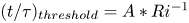 $(t/\tau )_{threshold} = A*Ri^{-1}$ fit with
  $A = 97.0$ and 218.8 for
  $Ga=80$ and
  $Ga=180$, respectively. The
  $O(Ri^{-1})$ fit in (b) is consistent with the case of an oblate spheroid in § 3.1.1.

3.2.2. Settling trajectory of a prolate spheroid in a stratified fluid
Similarly to the case of an oblate spheroid, stratification suppresses the oscillatory trajectories of a prolate spheroid in a homogeneous fluid at high  $Ga$. The settling trajectories of a prolate spheroid with
  $\mathcal {AR} = 2$ in a homogeneous and stratified fluid are displayed in figure 12. In a homogeneous fluid, the particle settles in a straight line at
  $Ga=80$ and in an oscillatory path at
  $Ga=180$. Since stratification results in a reduction of the settling velocity, the prolate spheroid stops at an earlier position as we increase the stratification strength. In addition, the oscillatory path observed for a prolate spheroid with
  $Ga=180$ in a homogeneous fluid disappears in a stratified fluid.
Trajectories of a prolate spheroid with  $\mathcal {AR}=2$ in a homogeneous and a stratified fluid for different
  $Ga$ and
  $Ri$. a)
  $Ga=80$, b)
  $Ga=180$ and c) a schematic summarizing the settling velocity, particle trajectory and the orientation in the two regimes observed in the settling motion. Left vertical axis and bottom horizontal axis indicate the spheroid position (solid line is the settling trajectory). Right vertical axis and top horizontal axis display the particle settling velocity vs time (dashed line is the settling velocity).

A prolate spheroid goes through two regimes, unlike the three regimes reported above for the settling of an oblate. In the first regime, denoted by  $I$, it oscillates about its broad-side on orientation as it settles. In this regime, the magnitude of the settling velocity is still higher than the threshold below which the spheroid starts to reorient. However, once the settling velocity drops below the threshold for the onset of reorientation, the particle starts to rotate from broad-side on to edge-wise orientation. This is regime
  $II$. Unlike an oblate spheroid which rotates quickly in regime
  $II$ and settles at a final edge-wise orientation in regime
  $III$, a prolate spheroid reorients slowly in regime
  $II$. Furthermore, the prolate spheroid does not reorient completely, but attains a final oblique orientation with
  $\theta$ between
  $0^{\circ }$ and
  $35^{\circ }$. The exact value of the final
  $\theta$ depends on
  $Ga$ and
  $Ri$ as explained before. The settling path along with the settling velocity are sketched in figure 12(c).
3.2.3. Why does a prolate spheroid reorients partially and only has two settling paths regimes in a stratified fluid?
As for the case of an oblate spheroid, we analyse the wake vortices to gain insight into the mechanisms leading to the reorientation of a prolate spheroid. The reasons for the deceleration and the reorientation of a prolate spheroid in a stratified fluid are similar to that of an oblate spheroid as will be discussed in this subsection. For a prolate spheroid settling in a homogeneous fluid, a single vortex attached to the particle is initially observed as in the case of an oblate spheroid. As we increase  $Ga$, this vortex grows in size. At low
  $Ga$ this vortical structure is still symmetric, however, it becomes helical, resulting in an instability for a prolate spheroid with
  $\mathcal {AR}=3$ for
  $Ga > 70$. As a result, a prolate spheroid with
  $\mathcal {AR}=3$ rotates about the vertical axis for
  $Ga > 70$ (Ardekani et al. Reference Ardekani, Costa, Breugem and Brandt2016). This is also clear in figure 12 as the prolate spheroid with
  $Ga=80$ settles in a straight line while the prolate spheroid with
  $Ga=180$ has an oscillatory path. As shown in Ardekani et al. (Reference Ardekani, Costa, Breugem and Brandt2016) the vortical structures for a prolate spheroid in a homogeneous fluid result in a broad-side on orientation.
The situation is completely different in the case of a prolate spheroid settling in a stratified fluid. In this configuration, the stratification suppresses the vertical motion of the fluid and prevents the particle from attaining any steady-state speed. In a stratified fluid, initially there is one vortex attached to the particle as shown in figure 13. As time passes, a part of this vortex detaches and remains predominantly on one side of the prolate spheroid as also shown in figure 13. As a result of this, there is a significant asymmetric low pressure region behind the prolate spheroid. This results in a torque which reorients the particle with its major axis aligned with the density gradient until it settles at its neutrally buoyant position. As discussed above, a prolate settles at an angle between  $0^{\circ }$ and
  $90^{\circ }$ depending on the Reynolds number.
Dimensionless iso-surfaces of Q-criterion equal to  $5 \times 10^{-4}$ for a prolate spheroid with
  $\mathcal {AR}=2$,
  $Ga=80$ and
  $Ri=5$ at equal time intervals of
  $t/\tau =28.65$;
  $t/\tau = 23.87$ for panel (a). The vortical structures identified by the positive Q-criterion are associated with a lower pressure region behind the particle.

We present for forces and torques acting on the prolate spheroid in figure 14. The net force and the force components,  $F_{h,z}$ and
  $F_{b,z}$ behave similarly to the case of an oblate spheroid discussed in § 3.1.3. High magnitude of the buoyancy force compared with the hydrodynamic drag explains the initial acceleration of the prolate. However, the buoyancy force decreases as the prolate sediments in a region with higher fluid density causing it to slow down. The gradual increase in the magnitude of the destabilizing buoyancy torque compared with the stabilizing hydrodynamic torque as the prolate velocity decreases explains the onset of reorientation to the edge-wise orientation below a threshold velocity as shown in figure 14(b). This is similar to an oblate spheroid, as shown in figure 7(b). However, a difference between the oblate and prolate spheroid case is found: the partial reorientation and the absence of regime III in the settling of a prolate spheroid.
(a) Forces acting on the prolate spheroid with  $Ga=80$ as it settles in a stratified fluid for different values of
  $Ri$ shown with different colours. The total force (solid line) can be split into two components, the hydrodynamic component (dashed line) and the buoyancy component (dotted line). (b) The
  $x$-component of the torque acting on a prolate spheroid with
  $Ga=80$ as it sediments in a stratified fluid with
  $Ri=5$ along with the
  $x$-component of the angular velocity. The net torque (solid line) is split into two components, the hydrodynamic torque (dotted line) which tries to orient the prolate in a broad-side on orientation (hence stabilizing) and the buoyancy component (dashed-dotted line) which is destabilizing and tries to reorient the prolate edge-wise. The reorientation starts once the magnitude of the hydrodynamic torque falls below the buoyancy torque which happens when the prolate velocity falls below the threshold for reorientation discussed in § 3.2.1.

The secondary motions of the spheroids provide a hint about the partial reorientation of a prolate spheroid. An oblate spheroid oscillates about the broad-side on orientation while a prolate spheroid does not oscillate about the broad-side on orientation as it attains terminal velocity in a homogeneous fluid (Ardekani et al. Reference Ardekani, Costa, Breugem and Brandt2016). Hence, if the inertial effects are strong enough, they can prevent the prolate spheroid from reorienting completely. This becomes clear if we compare the evolution of the buoyancy torque on an oblate spheroid and a prolate spheroid (figures 7b and 14b). Once the particle velocities fall below the threshold for the onset of reorientation, the destabilizing buoyancy torque on an oblate spheroid dominates for a longer time (4.5 units in dimensionless time which is enough to ensure that the oblate spheroid reorients completely) as compared with a prolate spheroid (1.75 units in dimensionless time which is not enough to reorient the spheroid completely) before they balance each other as the particle velocity approaches 0. Similar observations regarding complete/partial reorientation in the limit  $Re \to 0$ and
  $Ri \to 0$ were also made in a recent theoretical study (Varanasi, Marath & Subramanian Reference Varanasi, Marath and Subramanian2021) which hints at the role of the particle
  $\mathcal {AR}$ in determining the exact degree of reorientation.
To understand the reorientation mechanism, we again examine the  $x$-component of the vorticity generation (
 $\boldsymbol {\omega }_g$) due to the deformation of the isopycnals (figure 15). The dynamics is similar to what happens in the case of an oblate spheroid settling in a stratified fluid as discussed in § 3.1.3. The only difference is that the prolate spheroid reaches its neutrally buoyant location before it can reorient completely where it stops moving and rotating as seen in figures 10(c) and 10(d).
Evolution of the  $x$-component of the dimensionless vorticity generation term due to the misalignment of the density gradient vector with the direction of gravity,
  $\boldsymbol {\nabla }\rho _f \times \hat {\boldsymbol {k}}$, in the
  $x=0$ plane for a prolate spheroid with
  $\mathcal {AR}=2$,
  $Ga=80$ and
  $Ri=5$. The solid lines indicate dimensionless isopycnals or equal density lines separated by a value of
  $0.5$. Darker shade of grey indicates a higher density. The panels are snapshots (a–o) at specific time intervals with
  $t/\tau =$ 0, 4.77, 14.32, 23.87, 33.42, 42.97, 52.52, 62.07, 71.62, 81.17, 90.72, 100.27, 109.82, 119.37,and 219.65. Panel (a) shows the initial configuration and the panel (o) shows the settling configuration after the prolate stops.

3.2.4. Stratification drag on a prolate spheroid
Figure 16 shows the added drag due to stratification,  $C_D^S-C_D^H$ on a prolate spheroid sedimenting in a stratified fluid. The drag due to stratification behaves similarly to the case of an oblate spheroid discussed in § 3.1.4. The stratification drag on the prolate particle decreases as it accelerates.
  $C_D^S-C_D^H$ is minimum when it attains a peak velocity and starts to increase again as the buoyancy/stratification effects take over inertial effects and slow it down. As in the case of an oblate spheroid,
  $C_D^S-C_D^H$ scales as
  $\approx O(Fr(z)^{-4})$.
Added drag due to stratification,  $C_D^S-C_D^H$, for a prolate spheroid with
  $\mathcal {AR}=2$ as a function of the instantaneous particle Froude number,
  $Fr(z)$, for (a)
  $Ga=80$ and different stratification strengths. (b) Added drag at
  $Ri=5$ for different
  $Ga$. The arrows show the direction of increasing time and the filled dots show the simulation start time. The dashed pink line shows the
  $-4$ power line to indicate a
  $Fr(z)^{-4}$ scaling of
  $C_D^S-S_D^H$.

3.3. The effect of heat conductivity ratio $\kappa _r$ on the settling spheroid

For this study, we have chosen a no-flux boundary condition on the particle surface, i.e. the stratifying agent cannot diffuse inside the particle (adiabatic/impermeable or no flux) (Doostmohammadi & Ardekani Reference Doostmohammadi and Ardekani2015) and, as a consequence, pycnoclines must be normal to the particle surface. This is the case if the stratifying agent is salt or the particle is adiabatic. In this section, we investigate the settling dynamics when the fluid and particle temperature influence each other by changing the heat conductivity ratio  $k_r$. Figure 17 shows the settling dynamics of a particle having a non-zero
  $k_r$. For a small
  $k_r=0.001$, the settling dynamics of an oblate spheroid is similar to the case
  $k_r=0$. The velocity is slightly higher for
  $k_r=0.001$. The particle accelerates initially, attaining a peak velocity after which it decelerates and stops when it reaches its neutrally buoyant position. Also, as its velocity falls below a threshold, it reorients to an edge-wise orientation. Since the flux of the stratifying agent into/out of the particle is much slower than the settling dynamics of such a small value of
  $k_r$, the surrounding fluid is not subjected to any significant heat exchange-induced density change. As for the cases studied above, the particle settles in a fluid region with increasing density, its velocity decreases as the net buoyancy force acting on it increases and the isopycnals resist their deformation. No-flux boundary condition is typical for objects settling in a temperature or a salt-stratified fluid, e.g. plastics, metals, organisms, etc. (Hanazaki et al. Reference Hanazaki, Konishi and Okamura2009b; Doostmohammadi et al. Reference Doostmohammadi, Dabiri and Ardekani2014; Mehaddi et al. Reference Mehaddi, Candelier and Mehlig2018; Mercier et al. Reference Mercier, Wang, Péméja, Ern and Ardekani2020).
Effect of permeability of the particle of the stratifying agent on (a) the settling velocity,  $U_p(t)/U$, of a settling oblate spheroid with
  $\mathcal {AR}=1/3$, and (b) the orientation,
  $\theta$, for
  $Ri = 5$ and
  $10$. Here,
  $k = 0$ inside the particle means the stratifying agent cannot diffuse into/out of the spheroid. A non-zero value for
  $k$ inside the particle results in increasing the temperature and decreasing the density of the boundary layer. For a very small
  $k_r= 0.001$, the spheroid settling dynamics is similar to
  $k_r=0$ case. However, for a high
  $k_r=1$, the spheroid has a completely different settling dynamics. If the stratifying agent can diffuse inside the spheroid, then, the spheroid attains a terminal velocity and does not reorient. These results show that spheroids will reorient only in the case of salt-stratified fluid or an adiabatic particle and not in a temperature-stratified fluid with conductive particles.

The settling dynamics changes for a high  $k_r$ value. A high
  $k_r$ value implies significant heat exchanges between the two phases and results in a warmer fluid close to the particle surface. The warmer boundary layer with decreased density accelerates upwards and thus creates a downforce that prevents particles from deceleration. This scenario might occur in chemical processes, e.g. liquid fluidized beds, and marine snow settling in a temperature-stratified water. For
  $k_r=1$, the settling dynamics during the initial time for an oblate spheroid is similar to
  $k_r=0$ case, however, the particle does not keep decelerating as time passes in contrast to the case with
  $k_r=0$. For a high
  $k_r$, the particle attains a terminal velocity much like in the case of an oblate spheroid settling in a homogeneous fluid. The terminal velocity, however, decreases as we increase the stratification strength as shown in figure 17(a). Furthermore, the oblate spheroid does not reorient to an edge-wise orientation as its velocity does not fall below the threshold for the onset of reorientation instability, but settles in a broad-side on orientation as shown in figure 17(b). The same holds for a prolate spheroid as shown in figure 18. As discussed in §§ 3.1.3 and 3.2.3,
  $k_r=0$ implies that the isopycnals are orthogonal to the particle surface, which creates a net torque on the spheroid. For a higher
  $k_r$ value, the pycnoclines are not orthogonal to the particle surface and hence do not result in a significant destabilizing buoyancy torque,
  $T_b$, on the spheroid. Thus, we conclude that the no-flux boundary condition is essential to observe the reorientation of spheroids settling in a stratified fluid.
Effect of permeability of the particle to the stratifying agent on (a) the settling velocity,  $U_p(t)/U$, of a settling prolate spheroid with
  $\mathcal {AR}=2$, and (b) the orientation,
  $\theta$, for
  $Ri = 5$ and
  $10$. Here,
  $k = 0$ inside the particle means the stratifying agent cannot diffuse into the spheroid which results in no change in the density of the surrounding boundary layer. This is true in the case when the stratifying agent is salt. A non-zero value for
  $k$ inside the particle results in diffusing heat to the surrounding fluid and thus decreasing the density of the boundary layer. For a high
  $k_r=1$, the spheroid has a completely different settling dynamics, with the spheroid attaining a terminal velocity and not reorienting. These results show that spheroids will reorient only in the case of salt stratified fluid and not in a temperature-stratified fluid with conductive particles.

3.4. The effect of Prandtl number, $Pr$

The fluid  $Pr$ is one of the parameters that greatly influences the settling dynamics of particles in a stratified fluid.
  $Pr=\nu /\alpha$ quantifies the relative magnitude of momentum diffusivity and the thermal diffusivity. Previous numerical studies investigating the motion of isolated spheres in a stratified fluid concluded that changing the fluid
  $Pr$ leads to quantitative changes in the settling velocity (Doostmohammadi et al. Reference Doostmohammadi, Dabiri and Ardekani2014) and radius of downstream jet (Hanazaki et al. Reference Hanazaki, Konishi and Okamura2009b) but does not lead to any significant qualitative changes in the general trends and the overall behaviour. We find that similar observations hold true even for spheroid shaped particles settling in a stratified fluid.
We investigate the effect of increasing the fluid  $Pr$ from 0.7 (value corresponding to a temperature-stratified atmosphere) to 7 (value corresponding to a temperature-stratified water) on the settling velocity and the orientation of spheroids in a stratified fluid. Figure 19 show the settling velocity and orientation variations with time for an oblate (
 $\mathcal {AR}=1/3$) and a prolate (
 $\mathcal {AR}=2$) spheroid with fixed
  $Ga=80$,
  $Ri=5$ but for two different
  $Pr = 0.7$ and
  $7.0$. The data show that increasing the fluid
  $Pr$ to 7.0 only quantitatively changes the particle settling velocity and its orientation with time but does not change the general trends discussed in §§ 3.1.3 and 3.2.3 for
  $Pr=0.7$.
We observe that increasing the fluid  $Pr$ reduces the settling speed of the spheroids as in the case of spherical particles (Doostmohammadi et al. Reference Doostmohammadi, Dabiri and Ardekani2014). Also, the spheroids still reorient away for the broad-side on orientation once their velocity magnitude falls below a particular threshold. Interestingly, we observe that this threshold increases to
  $|U_p(t)/U| < 0.195$ for
  $Pr=7.0$ from
  $|U_p(t)/U| < 0.15$ for
  $Pr=0.7$ (figures 19a and 19c). Furthermore, increasing
  $Pr$ leads to a reduction in the time,
  $(t/\tau )_{threshold}$, for the onset of the spheroid reorientation and the time required for its reorientation as shown in figures 19(b) and 19(d). Increasing the value of
  $Pr$ results in slower stratifying agent diffusion and hence increases the influence of inertial or convective effects. As a result, the density boundary layer thickness which scales as
  $\delta _{\rho } \approx D/\sqrt {RePr}$ reduces with increasing
  $Pr$. The density gradients (
 $\boldsymbol {\nabla }\rho _f$ as introduced in (3.1)) near the particle surface scale as
  $\approx \gamma {D}/\delta _{\rho }=\gamma {\sqrt {RePr}}$. Thus, with increasing
  $Pr$, the magnitude of the density gradients near the particle surface increases. This results in a stronger buoyancy torque,
  $T_{b}$, on the spheroid in a fluid with a higher
  $Pr$ for a fixed
  $Ga$ and
  $Ri$ as can be seen in figure 20 for an oblate spheroid. This increases the velocity threshold and also reduces
  $(t/\tau )_{threshold}$ for the onset of spheroid reorientation.
Effect of the Prandtl number,  $Pr$, on the settling dynamics of an oblate (
 $\mathcal {AR}=1/3$, (a,b)) and a prolate (
 $\mathcal {AR}=2$, (c,d)) spheroid with
  $Ga=80$ settling in a stratified fluid with
  $Ri=5$. Here,
  $\kappa _r=0$. (a,c) Dimensionless settling velocity vs dimensionless time. Fluid
  $Pr$ quantitatively changes the settling velocity such that the settling velocity decreases with increasing
  $Pr$. However, the overall trend does not change, i.e. acceleration initially, attaining peak velocity, deceleration and finally particle stops at its neutrally buoyant level. Increasing
  $Pr$ to 7 from 0.7 also increases the threshold for the onset of reorientation to
  $|U_p(t)/U| < 0.195$ from
  $|U_p(t)/U| < 0.15$, respectively. (b,d) Particle orientation vs dimensionless time. Increasing the fluid
  $Pr$ leads to the onset of reorientation instability at an earlier time and also reduces the time interval in which the reorientation occurs. This shows that a fluid in which the convection dominates diffusion, the influence of the fluid stratification on the spheroid settling dynamics is stronger.

Variation in torque acting on an oblate spheroid with  $Ga=80$,
  $Ri=5$ and
  $\mathcal {AR}=1/3$ with time for two different
  $Pr$ values. Increasing the
  $Pr$ of the fluid results in a stronger and dominant buoyancy torque,
  $T_{b}$, on the spheroid for a fixed
  $Ga$ and
  $Ri$ which result in an earlier onset of the reorientation.

The results from this section prove that the basic physics behind the particle deceleration and reorientation is independent of the fluid  $Pr$ since it is rooted in the buoyancy force and torque as explained in §§ 3.1.3 and 3.2.3. Changing
  $Pr$ will change the magnitude of the buoyancy force and torque which results in a different peak velocity of the particles and a different time for the onset of the reorientation, but the particles still decelerate and reorient. Hence, the insights obtained from our study are also applicable at higher
  $Pr$ such as 7 for temperature-stratified water or Schmidt number of order 700 for salt stratified water. Our results also show a qualitative agreement with the experiments of disks settling in a salt-stratified fluid (Schmidt number
  $\approx 700$) (Mercier et al. Reference Mercier, Wang, Péméja, Ern and Ardekani2020) which showed that disks also decelerate as they settle and reorient which is what we observe as well.
4. Conclusions
We investigated the settling dynamics of anisotropic shaped particles in a density-stratified fluid using direct numerical simulations. The shapes considered are an oblate spheroid with  $\mathcal {AR}=1/3$ and a prolate spheroid with
  $\mathcal {AR}=2$. We vary the Reynolds number
  $Ga$ from 80 to 250 and the Richardson number
  $Ri$ from 0 to 10 while keeping the density ratio
  $\rho _r$ and Prandtl number
  $Pr$ constant. The results show that the settling dynamics of spheroids is significantly different in a stratified fluid than in a homogeneous fluid.
Initially, the spheroids accelerate from rest and reach a maximum velocity. The peak velocity attained by the particles increases with their  $Ga$ while decreases monotonically when increasing the stratification. After the settling velocity attain its peak value, stratification dominates over inertia, because the inertial effects are not enough to sustain the deformation of the isopycnals once the particle reaches its peak velocity. Hence, due to the tendency of the isopycnals to return to their original positions, the fluid experiences a resistance to its motion. This results in an increased drag and hence a deceleration of the particle until it stops at its neutrally buoyant position. This evolution of the settling velocity is similar to that of a spherical particle settling in a stratified fluid.
The fluid stratification alters the orientation of the spheroids compared with their orientations in a homogeneous fluid. The fluid stratification leads to reorientation instability as the particle settling velocity falls below a threshold. For the parameters considered here, the onset of the reorientation instability occurs at  $|U_p(t)/U| < 0.15$. Interestingly, the dimensionless threshold velocity for the onset of reorientation instability is found to be the same for the oblate and prolate spheroids. This value might be different for different values of the density ratio and the Prandtl number. As a result of this instability, an oblate spheroid settles with its broader side aligned with the direction of the stratification. On the other hand, a prolate spheroid reorients partially or fully depending on its
  $Ga$ and settles such that its longer edge is at an angle greater than
  $0^{\circ }$ and lower than
  $45^{\circ }$ with the horizontal direction. This is completely opposite to what happens in a homogeneous fluid as both an oblate and a prolate spheroid settle in a broad-side on orientation. Stratification also eliminates the oscillatory path instability observed for spheroids in a homogeneous fluid. This is due to the decreasing magnitude of the inertial effects as the particle decelerates while reaching regions of higher fluid density.
The asymmetry in the low pressure region behind the spheroids due to an asymmetric wake results in the onset of the reorientation instability. This asymmetry results from the asymmetric distribution of the vorticity generation term due to the misalignment of the density gradient vector with the vertical direction (baroclinic vorticity generation). As a result, the destabilizing buoyancy torque,  $T_b$, becomes dominant over the stabilizing hydrodynamic torque
  $T_h$ as the spheroid velocity falls below a threshold value causing the onset of reorientation instability. We also report that the spheroids will only reorient in the case when they are impermeable to the stratifying agent (
 $\kappa _r\ll 1$) which is true in the case of a salt stratification or an adiabatic particle. If the stratifying agent can diffuse (
 $\kappa _r\gg 0$) inside the particle, then the spheroid will not reorient and the settling dynamics is similar to that in a homogeneous fluid with stratification causing a reduction in the terminal velocity. We also find that increasing the fluid
  $Pr$ from 0.7 (temperature-stratified air) to 7.0 (temperature-stratified water) results in a stronger and dominant
  $T_b$ on the spheroids. As a results for
  $Pr=7.0$, the onset of reorientation occurs at a higher velocity threshold
  $|U_p(t)/U|<0.195$ and at an earlier time compared with case
  $Pr=0.7$. The results presented in this paper are a first contribution to the field of settling particles in a fluid, in particular for anisotropic particles and stratified fluids. As extensions of this work, it would be interesting to investigate the behaviour of particle suspensions, the effect of the aspect ratios and also extensively quantify the effect of
  $Pr$ as well as other particle shapes on the settling dynamics of particles in a stratified fluid.
Supplementary movies
Supplementary movies are available at https://doi.org/10.1017/jfm.2021.836.
Funding
A.M.A. would like to acknowledge financial support from National Science Foundation via grants CBET-1604423, and CBET-1705371. This work used the Extreme Science and Engineering Discovery Environment (XSEDE) (Towns et al. Reference Towns2014), which is supported by the National Science Foundation grant number ACI-1548562 through allocations TG-CTS180066 and TG-CTS190041. L.B. acknowledges FORMAS (Swedish research council for sustainable development) for their financial support through the JPI-Oceans MicroplastiX project.
Declaration of interests
The authors report no conflict of interest.
Appendix. Verification of domain size independence
In the absence of stratification, a domain with a vertical length much larger than  $Ga$ is needed to make sure that the wake does not have a strong effect on the settling of the particle by interacting with it. However, since fluid stratification suppresses the vertical motion, we can use a smaller vertical length for our domain. Here, we show that the chosen domain sizes are big enough to make sure that the particles do not interact with their wakes for the entire range of parameters explored in this study.
We find an excellent agreement between the terminal  $Re$ attained by a settling oblate spheroid with
  $\mathcal {AR} = 1/3$ in a homogeneous fluid, i.e.
  $Ri=0$, at different
  $Ga$ in a bigger domain (
 $15D \times 15D \times 125D$) and a smaller domain (
 $20D \times 20D \times 80D$), used for this study) as shown in table 2. This proves that there is no significant interaction between the particle wake and the particle as it settles and the used domain size is enough to resolve the particle dynamics. Additionally, figure 21 shows the velocity vs time evolution for a prolate spheroid with
  $\mathcal {AR} = 2$ with
  $Ga=180$ in a stratified fluid with
  $Ri=5$ in a bigger domain (
 $10D \times 10D \times 80D$) and a smaller domain (
 $10D \times 10D \times 40D$), used for this study). Again, this shows that there is no significant interaction between the particle and its wake and the domain size used for this study is enough to ensure accuracy for an affordable computational cost.
Comparison of velocity vs time for a prolate spheroid with  $\mathcal {AR}=2$ in two different domain sizes at
  $Ga=180$ and
  $Ri=5$. The error in the velocity using a smaller domain is negligible which means even a smaller domain gives accurate results but at a lower computational cost.

Comparison of terminal Reynolds numbers,  $Re_t$, with two different domain sizes in a homogeneous fluid, i.e.
  $Ri=0$ for an oblate spheroid with
  $\mathcal {AR}=1/3$ at different
  $Ga$. The values are in agreement, which means there is no significant interaction between the particle wake and the particle.


 Open access