





Introduction
Medical microwave imaging (MMWI) has gained increasing attention as a noninvasive diagnostic technique due to its low cost and use of nonionizing radiation [Reference Chandra, Zhou, Balasingham and Narayanan1–Reference Mousavi and Majedi7]. Conventional medical imaging modalities, including magnetic resonance imaging (MRI), computed tomography (CT), and positron emission tomography (PET), remain the gold standard for clinical diagnostics, offering high-resolution images. However, their widespread use is limited by high operational costs, sizable equipment, and, in the case of CT and PET, exposure to potentially harmful ionizing radiation. In contrast, MMWI provides a portable, safe, and cost-effective alternative that mitigates many drawbacks of MRI and CT, albeit with reduced spatial resolution. Among its various potential applications, brain imaging (particularly for stroke or tumor detection and follow-up) has emerged as one of the most promising areas for MMWI development [Reference Crocco, Karanasiou, James and Conceição2], highlighting its potential for rapid bedside diagnostic assessments.
Implementing MMWI entails solving an ill-posed and highly nonlinear inverse scattering problem [Reference Pastorino4], which poses a significant computational challenge. To address this, two main strategies have been proposed in the literature. The first strategy involves formulating a linearized version of the inverse problem to reconstruct qualitative, real-time images of the examined region. This approach is effective primarily for detecting small anomalies, under the assumption that prior patient-specific information about healthy tissues is available. In the absence of such information, however, qualitative MMWI reconstructions tend to be unreliable.
The second strategy, known as quantitative imaging, aims to reconstruct the complex permittivity distribution within the whole region of interest, including that of the stroke or tumor. Since biological tissues exhibit distinct permittivity values, this approach produces scan-like images reflecting tissue distribution. Quantitative imaging involves solving the full nonlinear inverse scattering problem, typically through iterative techniques such as inexact Newton methods [Reference Bozza, Estatico, Pastorino and Randazzo8, Reference Bozza and Pastorino9] or distorted Born iterative methods (DBIMs) [Reference Guo, Nguyen-Trong, AI-Saffar, Stancombe, Bialkowski and Abbosh10–Reference Islam, Islam and Kiourti14]. However, these methods are often computationally prohibitive due to their iterative nature. More critically, they are susceptible to false solutions, estimates that satisfy the measured data but deviate from the true permittivity distribution. Both excessive computational cost and the risk of false reconstructions can be mitigated by employing patient-specific background models as initial estimates in the optimization process.
Based on the above discussion, having an appropriate patient-specific model is crucial for improving performance in both qualitative and quantitative inverse scattering approaches. In qualitative imaging, the model must be sufficiently accurate to enable rapid detection of subtle tissue variations, such as tumor growth or disease progression. In quantitative imaging, where the aim is to capture finer tissue changes, the model serves as a reliable initialization that guides the optimization process toward the true solution, accelerates convergence, and significantly reduces the number of required iterations, making these algorithms more practical for real-time diagnostic applications.
The concept of a patient-specific background model was first introduced at the EuCAP 2025 Conference and published in its proceedings [Reference Ninković, Kovačević, Kolundžija, Scapaticci, Crocco and Nikolić Stevanović15], where preliminary results were reported. In that work, initial head images were reconstructed using a linear inverse-scattering model based on the Born approximation and regularized with polynomial basis functions representing the contrast. These images were subsequently segmented and converted into a four-domain phantom, with the permittivities of each domain estimated using a suitably formulated DBIM approach. The techniques for phantom generation from MMWI images are further refined and extended in Ninković et al. [Reference Ninković, Kovačević, Kolundžija, Crocco and Stevanović16], along with a stroke detection analysis that could benefit from the patient-specific background model.
In this work, we introduce several key improvements over Nincović et al. [Reference Ninković, Kovačević, Kolundžija, Scapaticci, Crocco and Nikolić Stevanović15, Reference Ninković, Kovačević, Kolundžija, Crocco and Stevanović16]. The primary advancement lies in the use of conformal basis functions, rather than polynomial basis functions, to model the unknown contrast. Specifically, a combination of low-order spherical harmonics is employed to capture angular deviations from the outer head geometry, while radial pulse functions are used to represent the rapidly varying permittivity along the radial direction. This formulation enables a more accurate delineation of tissue boundaries, improves reconstruction accuracy, and reduces the number of required basis functions, thereby alleviating the ill-posedness of the problem.
In addition, a more realistic and complex phantom is considered compared to Ninković et al. Reference Ninković, Kovačević, Kolundžija, Scapaticci, Crocco and Nikolić Stevanović15, Reference Ninković, Kovačević, Kolundžija, Crocco and Stevanović16], incorporating an additional tissue layer corresponding to cerebrospinal fluid (CSF). Finally, the robustness of the proposed method under practical conditions is evaluated by introducing noise into the scattering parameters across a range of signal-to-noise ratio (SNR) levels.
Thus, the main outcome of this work is an improved four-domain phantom, together with corresponding estimates of tissue permittivities. The proposed phantom can serve as a fast, patient-specific approximation of a healthy head and can be integrated as an initial modeling step within a clinical workflow, enabling rapid stroke detection even when only limited prior information, such as the outer head shape, is available. This capability is particularly valuable in time-critical scenarios, when conventional imaging modalities may not be readily accessible.
The remainder of this paper is organized as follows: The “Parametric modeling of the permittivity distribution” section introduces the selected parametric model for representing the permittivity distribution. The “MMWI scenario” section details the considered MMWI scenario. In the “Distorted Born iterative method” section, the applied formulation of DBIM is outlined. The obtained results for the numerical example are presented in the “Numerical example” section. Finally, the “Conclusion” section provides the concluding remarks.
Parametric modeling of the permittivity distribution
To mitigate the ill-posedness of the inverse problem, it is advantageous to represent the unknown permittivity distribution using suitable basis functions, thereby reducing the dimensionality of the solution space. In the upper head region, head tissues are approximately conformal to the overall head shape. Therefore, it is reasonable to employ basis functions that follow this outer geometry while still accommodating variations, which can be effectively modeled using low-order spherical harmonics. Each point on the head surface can be represented as
 \begin{equation}{R_{\text{s}}}\left( {\theta ,\varphi } \right) \approx \sum _{l = 0}^L \sum _{m = - l}^l {a_{lm}}Y_l^m\left( {\theta ,\varphi } \right),\end{equation}
where  $Y_l^m\left( {\theta ,\varphi } \right)$ is the spherical harmonic of the degree l and order m, L is the maximal degree of spherical harmonics, and alm are the expansion coefficients. Similarly, the permittivity distribution, represented as a three-dimensional (3D) function in the spherical coordinate system,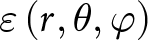 $\varepsilon \left( {r,\theta ,\varphi } \right)$, can be approximated by a series of orthogonal basis functions formed as the product of radial functions – which model radial dependence – and spherical harmonics, which capture angular dependence. This expansion takes the form:
 \begin{equation}
\varepsilon (r,\theta ,\varphi) \approx \sum_{n = 1}^{N} \sum_{l = 0}^{L} \sum_{m = - l}^{l} c_{nlm}p_{n}({\hat r})Y_{l}^{m} ({\theta ,\varphi }),
\end{equation}
\begin{equation}
\varepsilon (r,\theta ,\varphi) \approx \sum_{n = 1}^{N} \sum_{l = 0}^{L} \sum_{m = - l}^{l} c_{nlm}p_{n}({\hat r})Y_{l}^{m} ({\theta ,\varphi }),
\end{equation}where  ${c_{nlm}}$ are the corresponding expansion coefficients, $\hat r$ is the normalized radial coordinate
 \begin{equation}\hat r\left( {r,\unicode{x03B8} ,\varphi } \right) = \frac{{{R_{\text{s}}}\left( {\theta ,\varphi } \right) - r}}{{{R_{\text{s}}}\left( {\theta ,\varphi } \right)}},\end{equation}
 (i.e., the normalized radial distance from the head surface),  ${p_n}\left( {\hat r} \right)$ are the radial pulse or indicator basis functions, $n = 1, \ldots ,N$, defined as
 \begin{equation}{p_n}\left( {\hat r} \right) = \left\{ {\begin{array}{*{20}{c}}
{1,\,\,\,} \\
{0,\,\,\,}
\end{array}} \right.\begin{array}{*{20}{c}}
{{\text{if }}r' \in \left[ {(n - 1)/N,\;n/N} \right)} \\
{{\text{otherwise}}}
\end{array}.\end{equation}
\begin{equation}{p_n}\left( {\hat r} \right) = \left\{ {\begin{array}{*{20}{c}}
{1,\,\,\,} \\
{0,\,\,\,}
\end{array}} \right.\begin{array}{*{20}{c}}
{{\text{if }}r' \in \left[ {(n - 1)/N,\;n/N} \right)} \\
{{\text{otherwise}}}
\end{array}.\end{equation} In the numerical implementation, the space is uniformly divided into K voxels, with each voxel having the constant permittivity, εk,  $k = 1, \ldots ,K$. In matrix form, this can be written as
 \begin{equation}{\boldsymbol{\varepsilon }} = {\mathbf{Hc}},\end{equation}
where ε is the vector of unknown permittivities
 \begin{equation}{\boldsymbol{\varepsilon }} = {\left[ {\begin{array}{*{20}{c}}
{{\varepsilon _1}}& \ldots &{{\varepsilon _K}}
\end{array}} \right]^{\text{T}}},\end{equation}
\begin{equation}{\boldsymbol{\varepsilon }} = {\left[ {\begin{array}{*{20}{c}}
{{\varepsilon _1}}& \ldots &{{\varepsilon _K}}
\end{array}} \right]^{\text{T}}},\end{equation}  ${\mathbf{c}}$ is the vector of the unknown coefficients
 \begin{equation}{\mathbf{c}} = {\left[ {\begin{array}{*{20}{c}}
{{c_1}}& \ldots &{{c_Q}}
\end{array}} \right]^{\text{T}}},\end{equation}
\begin{equation}{\mathbf{c}} = {\left[ {\begin{array}{*{20}{c}}
{{c_1}}& \ldots &{{c_Q}}
\end{array}} \right]^{\text{T}}},\end{equation}and Q is the total number of coefficients  $Q = N{\left( {L + 1} \right)^2}$. In (7), we used simplified notation cj = cnlm, where j is a single index corresponding to a triplet (n, l, m), $j = 1,{\text{ }} \ldots ,{\text{ }}Q$. Furthermore, H is the transformation matrix whose elements are calculated as
 \begin{equation}{\mathbf{H}}(k,j) = {p_n}\left( {{{\hat r}_k}} \right)Y_l^m\left( {{\theta _k},{\varphi _k}} \right),\,k = 1,{\text{ }} \ldots ,{\text{ }}K,\,\,j = 1,{\text{ }} \ldots ,{\text{ }}Q,\end{equation}
where  $\left( {{r_k},{\theta _k},{\varphi _k}} \right)$ are the spherical coordinates of the kth voxel and ${\hat r_k} = \frac{{{R_{\text{s}}}\left( {{\theta _k},{\varphi _k}} \right) - {r_k}}}{{{R_{\text{s}}}\left( {{\theta _k},{\varphi _k}} \right)}}$.
MMWI scenario
Figure 1 (a) illustrates an MMWI scenario, consisting of an array of antennas in close contact with the head. In the considered example, the head model comprises six homogeneous tissues. The assumed initial background model, shown in Fig. 1(b), represents a homogeneous head with a permittivity equal to that of brain tissue and includes a thin layer corresponding to the skin. The underlying physical model is the scattering equation, which, under the Born approximation, is given by [Reference Nikolova17, Reference Nikolić Stevanović and Đorđević18]:
 \begin{equation}\begin{gathered}
{\Delta _{{S_{ij}}}}\, \approx - \frac{{{\text{j}}\omega }}{{2{a_i}{a_j}}}\mathop\int_{v'} {\Delta \varepsilon (\boldsymbol{r}'){\boldsymbol{E}}_{\text{i}}^i} (\boldsymbol{r}')\cdot\,\boldsymbol{E}_{\text{i}}^j\,(\boldsymbol{r}'){\text{d}}v',i,j = {\text{1}},\ldots,M,
\end{gathered} \end{equation}
\begin{equation}\begin{gathered}
{\Delta _{{S_{ij}}}}\, \approx - \frac{{{\text{j}}\omega }}{{2{a_i}{a_j}}}\mathop\int_{v'} {\Delta \varepsilon (\boldsymbol{r}'){\boldsymbol{E}}_{\text{i}}^i} (\boldsymbol{r}')\cdot\,\boldsymbol{E}_{\text{i}}^j\,(\boldsymbol{r}'){\text{d}}v',i,j = {\text{1}},\ldots,M,
\end{gathered} \end{equation} \begin{equation}
\Delta S_{i,j} = S_{i,j} - S_{i,j}^0 , \Delta {\varepsilon _k} = {\varepsilon _k} - {\varepsilon _{k,{\text{b}}}},
\end{equation}
\begin{equation}
\Delta S_{i,j} = S_{i,j} - S_{i,j}^0 , \Delta {\varepsilon _k} = {\varepsilon _k} - {\varepsilon _{k,{\text{b}}}},
\end{equation}(a) Brain imaging scenario. (b) Initial background model.

Figure (1) Long description
The image A shows a head model with an array of antennas in close contact. The internal structures, including the brain, are visible with a mesh overlay. The image B shows a similar head model with a homogeneous appearance, also with antennas, but without internal details visible. Both diagrams illustrate different modeling approaches for the head, with antennas positioned around the top and sides.
where  ${s_{ij}}$ and $s_{ij}^0$ are the transmission coefficients between the ith and jth antennas, computed or measured for the actual system and assumed background, respectively, ε is the unknown head permittivity, ${\varepsilon _{\text{b}}}$ is the known permittivity of the background model, $\Delta \varepsilon $ is the permittivity difference, ${\mathbf{r}}'$is the position vector of a point inside the head, ${\mathbf{E}}_{\text{i}}^{i\left( j \right)}$ is the electric field vector computed in the background model when the i(j)th antenna is transmitting, ${a_{i(j)}}$ is the complex amplitude of the incident power wave at the i(j)th port, M is the size of the array, v′ is the known volume occupied by the head, and $\omega $ is the angular frequency.
In the discrete case, (9) becomes
 \begin{equation}{\Delta _{{S_{ij}}}} \approx - - \frac{{{\text{j}}\omega \Delta v}}{{2{a_i}{a_j}}}\sum ^K_{K = 1} \Delta {\varepsilon _k}\,\boldsymbol{E}_{\text{i}}^i({\boldsymbol{t}_k})\cdot\,\boldsymbol{E}_i^j({\boldsymbol{t}_k}),\,i,j = 1,\ldots.,M\end{equation}
 \begin{equation}\Delta {\varepsilon _k} = {\varepsilon _k} - {\varepsilon _{k,{\text{b}}}},\,k = 1, \ldots ,K,\end{equation}
 where  ${{\mathbf{t}}_k}$ is the position vector of the center of the kth voxel, and ${{\varepsilon }_k}$, and ${{\varepsilon }_{k,{\text{b}}}}$ are the constant permittivities of the kth voxel in the actual head and background model, respectively, $\Delta {{\varepsilon }_k}$ is their difference, $\Delta v$ is the volume of each voxel, and K is the total number of voxels into which the occupied volume is divided. In matrix form, (10) becomes
 \begin{equation}\Delta {\mathbf{s}} = {\mathbf{L}}\Delta {\boldsymbol{\varepsilon }},\end{equation}
with
 \begin{equation}\Delta {\mathbf{s}} = {\left[ {\begin{array}{*{20}{c}}
{\Delta {s_{1,1}}}&{\Delta {s_{1,2}}}& \cdots &{\Delta {s_{M,M}}}
\end{array}} \right]^{\text{T}}},\end{equation}
\begin{equation}\Delta {\mathbf{s}} = {\left[ {\begin{array}{*{20}{c}}
{\Delta {s_{1,1}}}&{\Delta {s_{1,2}}}& \cdots &{\Delta {s_{M,M}}}
\end{array}} \right]^{\text{T}}},\end{equation} \begin{equation}{{\mathbf{L}}^{}} = - \frac{{{\text{j}}\omega \Delta v}}{2} \cdot \left[ {\begin{array}{*{20}{c}}
{\frac{{{\mathbf{E}}_{\text{i}}^1\left( {{{\mathbf{t}}_1}} \right) \cdot {\mathbf{E}}_{\text{i}}^1\left( {{{\mathbf{t}}_1}} \right)}}{{{a_1}{a_1}}}}& \ldots &{\frac{{{\mathbf{E}}_{\text{i}}^1\left( {{{\mathbf{t}}_L}} \right) \cdot {\mathbf{E}}_{\text{i}}^1\left( {{{\mathbf{t}}_L}} \right)}}{{{a_1}{a_1}}}} \\
{\frac{{{\mathbf{E}}_{\text{i}}^1\left( {{{\mathbf{t}}_1}} \right) \cdot {\mathbf{E}}_{\text{i}}^2\left( {{{\mathbf{t}}_1}} \right)}}{{{a_1}{a_2}}}}& \vdots &{\frac{{{\mathbf{E}}_{\text{i}}^1\left( {{{\mathbf{t}}_L}} \right) \cdot {\mathbf{E}}_{\text{i}}^2\left( {{{\mathbf{t}}_L}} \right)}}{{{a_1}{a_2}}}} \\
\vdots & \vdots & \vdots \\
{\frac{{{\mathbf{E}}_{\text{i}}^M\left( {{{\mathbf{t}}_1}} \right) \cdot {\mathbf{E}}_{\text{i}}^M\left( {{{\mathbf{t}}_1}} \right)}}{{{a_M}{a_M}}}}& \ldots &{\frac{{{\mathbf{E}}_{\text{i}}^M\left( {{{\mathbf{t}}_L}} \right) \cdot {\mathbf{E}}_{\text{i}}^M\left( {{{\mathbf{t}}_L}} \right)}}{{{a_M}{a_M}}}}
\end{array}} \right],\end{equation}
\begin{equation}{{\mathbf{L}}^{}} = - \frac{{{\text{j}}\omega \Delta v}}{2} \cdot \left[ {\begin{array}{*{20}{c}}
{\frac{{{\mathbf{E}}_{\text{i}}^1\left( {{{\mathbf{t}}_1}} \right) \cdot {\mathbf{E}}_{\text{i}}^1\left( {{{\mathbf{t}}_1}} \right)}}{{{a_1}{a_1}}}}& \ldots &{\frac{{{\mathbf{E}}_{\text{i}}^1\left( {{{\mathbf{t}}_L}} \right) \cdot {\mathbf{E}}_{\text{i}}^1\left( {{{\mathbf{t}}_L}} \right)}}{{{a_1}{a_1}}}} \\
{\frac{{{\mathbf{E}}_{\text{i}}^1\left( {{{\mathbf{t}}_1}} \right) \cdot {\mathbf{E}}_{\text{i}}^2\left( {{{\mathbf{t}}_1}} \right)}}{{{a_1}{a_2}}}}& \vdots &{\frac{{{\mathbf{E}}_{\text{i}}^1\left( {{{\mathbf{t}}_L}} \right) \cdot {\mathbf{E}}_{\text{i}}^2\left( {{{\mathbf{t}}_L}} \right)}}{{{a_1}{a_2}}}} \\
\vdots & \vdots & \vdots \\
{\frac{{{\mathbf{E}}_{\text{i}}^M\left( {{{\mathbf{t}}_1}} \right) \cdot {\mathbf{E}}_{\text{i}}^M\left( {{{\mathbf{t}}_1}} \right)}}{{{a_M}{a_M}}}}& \ldots &{\frac{{{\mathbf{E}}_{\text{i}}^M\left( {{{\mathbf{t}}_L}} \right) \cdot {\mathbf{E}}_{\text{i}}^M\left( {{{\mathbf{t}}_L}} \right)}}{{{a_M}{a_M}}}}
\end{array}} \right],\end{equation} \begin{equation}\Delta {\boldsymbol{\varepsilon }} = {\left[ {\begin{array}{*{20}{c}}
{\Delta {\varepsilon _1}}& \ldots &{\Delta {\varepsilon _L}}
\end{array}} \right]^{\text{T}}}.\end{equation}
\begin{equation}\Delta {\boldsymbol{\varepsilon }} = {\left[ {\begin{array}{*{20}{c}}
{\Delta {\varepsilon _1}}& \ldots &{\Delta {\varepsilon _L}}
\end{array}} \right]^{\text{T}}}.\end{equation}We express the permittivity difference vector (12c) using the adopted basis functions (5) as
 \begin{equation}\Delta {\boldsymbol{\varepsilon }} = {\mathbf{Hc}}.\end{equation}
When (13) is inserted into (11), we obtain the final system of equations relating the measurements and the polynomial coefficients
 \begin{equation}{\boldsymbol{\Delta s}} = {\mathbf{Ac}},\end{equation}
where  ${\mathbf{A}} = {\mathbf{LH}}$. To solve (14), the Tikhonov regularization is adopted. The corresponding cost function is
 \begin{equation}J = \left\| {{\boldsymbol{\Delta s}} - {\mathbf{Ac}}} \right\|_2^2 + \lambda \left\| {{\mathbf{Hc}}} \right\|_2^2\end{equation}
where  $\lambda $ is regularization coefficient. The solution of (15) is
 \begin{equation}{\boldsymbol{\tilde c}} = {\left( {{{\mathbf{A}}^{\text{H}}}{\mathbf{A}} + \lambda {{\mathbf{H}}^{\text{H}}}{\mathbf{H}}} \right)^{ - 1}}{{\mathbf{A}}^{\text{H}}}{\boldsymbol{\Delta s}}\end{equation}
and the estimated permittivity vector is
 \begin{equation}\tilde{\boldsymbol{\varepsilon }} = \mathbf{H}\boldsymbol{\tilde c} + {{\boldsymbol{\varepsilon }}_{\text{b}}}\end{equation}
where
 \begin{equation}{{\boldsymbol{\varepsilon }}_{\text{b}}} = {\left[ {\begin{array}{*{20}{c}}
{{\varepsilon _{{\text{1,b}}}}}& \ldots &{{\varepsilon _{K{\text{,b}}}}}
\end{array}} \right]^{\text{T}}},\end{equation}
\begin{equation}{{\boldsymbol{\varepsilon }}_{\text{b}}} = {\left[ {\begin{array}{*{20}{c}}
{{\varepsilon _{{\text{1,b}}}}}& \ldots &{{\varepsilon _{K{\text{,b}}}}}
\end{array}} \right]^{\text{T}}},\end{equation}  ${{\boldsymbol{\varepsilon }}_{\text{b}}}$ is the background permittivity vector. Based on the approximate solution (17), we extract information about the skull by assuming that all voxels with intensity below a chosen threshold correspond to the skull, due to its low permittivity. Once the skull is identified, its interior is assumed to represent the brain. The model is then completed by adding a thin surface layer, conformal to the outer head shape. As a result, a parametric head model comprising four homogenous tissues is obtained.
Distorted Born iterative method
Once the parametric head model is obtained, we calculate the complex permittivities of its domains using the DBIM.
The DBIM has been widely employed in MMWI, with notable applications such as the following. A calibrated, frequency-division DBIM-based two-dimensional (2D) microwave tomography algorithm for head imaging was validated on head phantoms and healthy volunteers [Reference Guo, Nguyen-Trong, AI-Saffar, Stancombe, Bialkowski and Abbosh10]. A 3D adaptive clustering DBIM approach for stroke detection was evaluated using a head scanner system and head phantoms, under the assumption that the number of tissues in the imaged domain and their approximate electromagnetic properties are known [Reference Guo, Khosravi-Farsani, Stancombe, Bialkowski and Abbosh11]. A brain stroke detection algorithm using the DBIM with two-step iterative shrinkage thresholding (DBIM-TwIST) was experimentally validated on a 2D head phantom, encircled by a ring of antennas [Reference Karadima, Lu, Sotiriou and Kosmas12]. A resolution-enhanced DBIM with a region-of-interest limitation scheme for microwave breast imaging yielded promising results on 2D numerical models [Reference Suzuki and Kidera13]. The extended Born iterative method, incorporating a localized nonlinear approximation, achieved fast convergence and robust anomaly detection in realistic 2D numerical models of stroke and breast tumors [Reference Islam, Islam and Kiourti14]. Unlike previous approaches, we apply the DBIM using previously estimated tissue boundaries, reducing the number of unknowns to the number of tissues without requiring patient-specific a priori information.
General DBIM formulation
The DBIM solves (10) by iteratively updating the estimated values of the permittivities in the background model  ${{\varepsilon }_{k,b}}$, and values of $\Delta {s_{ij}}$ and ${\mathbf{E}}_i^{i\left( j \right)}$ corresponding to the estimates of the ${{\varepsilon }_{k,{\text{b}}}}$, where the background model is obtained by the procedure described in the previous section. To start the DBIM algorithm, the permittivity values $\varepsilon _{1,{\text{b}}}^{(1)},{\text{ }}\varepsilon _{2,{\text{b}}}^{(1)},{\text{ }}\ldots{\text{, }}\varepsilon _{K,{\text{b}}}^{(1)}$, must be initialized.
In the lth iteration, the linear system of equations (11) is
 \begin{equation}\Delta {{\mathbf{s}}^{(l)}} = {{\mathbf{L}}^{(l)}}\Delta {{\boldsymbol{\varepsilon }}^{(l)}},\end{equation}
where  $\Delta {{\mathbf{s}}^{(l)}}$, ${{\mathbf{L}}^{(l)}}$, and $\Delta {{\boldsymbol{\varepsilon }}^{(l)}}$ are values of matrices in the lth iteration.
The system (19) is solved using truncated singular value decomposition. The regularized solution is
 \begin{equation}\Delta {{\boldsymbol{\varepsilon }}^{\left( l \right)}} = \sum\limits_{n = 1}^{{n_{\max }}} {\frac{1}{{{\sigma _n}}}\left( {{\mathbf{u}}_n^{\text{H}} \cdot \Delta {{\mathbf{s}}^{\left( l \right)}}} \right){{\mathbf{v}}_n}} {\text{ ,}}\end{equation}
where  ${{\mathbf{u}}_n}$, and ${{\mathbf{v}}_n}$ are the singular vectors of matrix ${{\mathbf{L}}^{\left( l \right)}}$, ${\sigma _n}$ are the corresponding singular values, and ${n_{\max }}$ is the truncation index, calculated using condition $10{\log _{10}}\left( {\frac{{{\sigma _{{n_{\max }}}}}}{{{\sigma _1}}}} \right) \lt - 20\;{\text{dB}}$. The permittivity estimate in the next iteration is calculated as
 \begin{equation}{{\boldsymbol{\hat \varepsilon }}^{\left( {l + 1} \right)}} = {{\boldsymbol{\hat \varepsilon }}^{\left( l \right)}} + \Delta {{\boldsymbol{\hat \varepsilon }}^{\left( l \right)}}.\end{equation}
 The DBIM algorithm is stopped when the magnitude of each member of the vector  $\Delta {{\boldsymbol{\varepsilon }}^{\left( l \right)}}$ is smaller than some predefined threshold (set to 0.01 in all experiments presented in this work) or when the maximum number of iterations is reached.
DBIM formulation with known domain boundaries
If the domain of interest can be partitioned into subdomains of homogeneous permittivity with known boundaries, the number of unknown parameters is reduced to the number of these subdomains. The corresponding measurement model can then be expressed as
 \begin{equation}\Delta {{\mathbf{s}}^{\left( l \right)}} = {{\mathbf{L}}^{\left( l \right)}}{\mathbf{W}}\,\Delta {{\boldsymbol{\varepsilon }}^{\left( l \right)}},\end{equation}
where W is the transformational matrix of size  $K \times S,$ and S is the number of subdomains. The (k, j) element of W equals 1 if the kth voxel belongs to the jth domain and 0 otherwise. The unknown vector is, thus,
 \begin{equation}\Delta {{\boldsymbol{\varepsilon }}^{(l)}} = {\left[ {\begin{array}{*{20}{c}}
{\Delta \boldsymbol{\varepsilon} _1^{(l)}}&{\Delta \boldsymbol{\varepsilon} _2^{(l)}}& \cdots &{\Delta \boldsymbol{\varepsilon} _S^{(l)}}
\end{array}} \right]^{\text{T}}},\end{equation}
\begin{equation}\Delta {{\boldsymbol{\varepsilon }}^{(l)}} = {\left[ {\begin{array}{*{20}{c}}
{\Delta \boldsymbol{\varepsilon} _1^{(l)}}&{\Delta \boldsymbol{\varepsilon} _2^{(l)}}& \cdots &{\Delta \boldsymbol{\varepsilon} _S^{(l)}}
\end{array}} \right]^{\text{T}}},\end{equation}where  $\Delta \varepsilon _j^{(l)}$ refers to the contrast of the jth domain in the lth iteration.
Numerical example
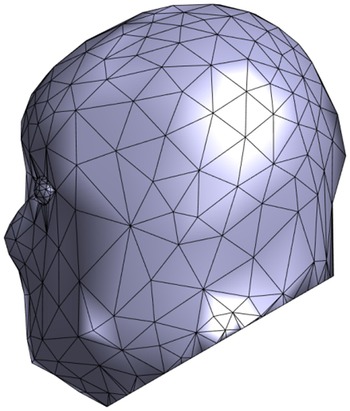
As a numerical example, a realistic head phantom shown in Fig. 1 (a) is considered. The phantom is based on the NEVA female anatomical model [19] and adapted for MMWI applications within the WIPL-D Pro simulation environment [20]. The phantom consists of six homogeneous tissue layers, as illustrated in Fig. 1(a), with their respective permittivity values listed in Table 1. We assume that the outer surface of the phantom is known and given by a triangular mesh in Fig. 2. In reality, geometrical information is needed only in the upper part of the head below the helmet. The measurement setup comprised a helmet equipped with 21 closely spaced trapezoidal patch antennas, each operating at 1 GHz and optimized for performance in the presence of the head model. Further details regarding the head phantom and the measurement system configuration are provided in Singh et al. [Reference Singh, Ninkovic, Tasic, Stevanovic and Kolundzija21].
Triangular mesh of the skin layer of the phantom from Figure 1.

Figure 2 Long description
The image shows a triangular mesh model representing a head phantom. The mesh consists of numerous interconnected triangles forming the surface of the head. The structure is detailed, with the triangles varying in size and shape, creating a geometric pattern across the surface. The mesh covers the entire head, including the facial region and provides a three-dimensional representation of the head's contours and features.
Complex permittivity of head tissues @ 1 GHz

Table 1 Long description
The table measures the complex permittivity of various head tissues at a frequency of 1 GHz. Cerebrospinal fluid exhibits the highest complex permittivity, indicating a strong ability to store and dissipate electrical energy. In contrast, fat shows the lowest values, suggesting minimal interaction with electromagnetic fields. Skin and soft tissue have similar permittivity values, both significantly higher than that of the skull. The brain's permittivity is notably lower than cerebrospinal fluid but higher than fat and skull. These differences highlight the varying electromagnetic properties of head tissues, which are crucial for medical imaging and treatment planning.
All results presented in this paper are generated using a desktop computer: Intel Core i7-9700 CPU @3 GHz, NVIDIA GeForce GTX 750 Ti GPU, with 32 GB of RAM under the Windows 10 operating system.
Parametric model creation
The first step involves extracting points on the head surface within a defined region of interest where the skull and overlying tissues are approximately conformal. These points are then used to construct a closed surface. Since the triangular mesh, shown in Fig. 2, is relatively rough, we first interpolate additional surface points and subsequently extract those located near the helmet, as illustrated in Fig. 3(a). To ensure geometric uniformity, the boundary points in each slice are then mapped onto a uniform angular grid in polar coordinates, providing a consistent number of points per layer. Finally, to complete the closed surface, additional points are generated by shrinking the lowest layer and translating it downward, as shown in Fig. 3(b). The resulting extrapolated surface points serve as the matching points for the spherical approximation, the outcome of which is shown in Fig. 3 (c). In computing the spherical harmonic approximation, we assume that the xy-plane coincides with the layer where the head has the maximum perimeter. The expansion coefficients are used for calculating the normalized radius in (2).
Computation of the boundary surface. (a) Portion of the head surface used for mapping, with corresponding surface points. (b) Extrapolated surface points arranged on a uniform polar grid in each horizontal cross-section. (c) Reconstructed boundary surface. (d) Final set of points used for imaging.

Figure 3 Long description
Image A shows a portion of the head surface with corresponding surface points highlighted. Image B displays extrapolated surface points arranged on a uniform polar grid in each horizontal cross-section. Image C illustrates the reconstructed boundary surface using a triangular mesh. Image D presents the final set of points used for imaging, completing the closed surface reconstruction.
For microwave imaging, we use a uniform 3D grid, within the defined closed surface and above  ${z_{\min }} = - 0.02\;{\text{m}}$. This resulted in a total of 34,947 voxels of side length 4 mm, as shown in Fig. 2 (d). Lower regions were omitted due to insufficient field penetration, which limited their utility for reliable imaging.
Regarding permittivity expansion (2), along the radial direction, we set  $N = 25$ pulses for radial variation, and $L = 3$ for the maximal order of the spherical harmonics expansion. The number of pulses is selected as a trade-off between spatial resolution and numerical stability. The order of the spherical harmonics is kept low to preserve the conformality of tissues, while still allowing a certain degree of flexibility.
As the assumed background model, the two-tissue head phantom presented in Fig. 1 (b) was used. The outer tissue mimicked skin and fat, and its permittivity was set to 28.50–j8.96, as the average value of the skin and fat permittivity values. The adopted thickness was 3.5 mm. The permittivity of the inner tissue was set to the value of the brain permittivity.
The results for selected cross-sections (out of 30, ordered from the lowest to the highest layer) are shown in Fig. 4. In each image pair, the right-hand image represents the reconstructed contrast (real part of the permittivity difference), while the left-hand image shows the true contrast, both relative to the adopted background model.
Reconstructed permittivity differences in various horizontal cross-sections (z-cuts), on the right, and corresponding ground truth, on the left.

Figure 4 Long description
Twelve plots display permittivity differences across horizontal cross-sections labeled z equals z subscript 7, z equals z subscript 9, z equals z subscript 11, z equals z subscript 13, z equals z subscript 15, z equals z subscript 17, z equals z subscript 19, z equals z subscript 21, z equals z subscript 23 and z equals z subscript 25. Each plot has axes labeled x left parenthesis m right parenthesis and y left parenthesis m right parenthesis, with a color scale indicating permittivity differences. The plots show variations in permittivity across different layers, with distinct patterns and color distributions in each cross-section.
The influence of the number of pulses and the maximal spherical harmonics order was examined through a sensitivity analysis. The reconstruction results for different parameter choices are illustrated in Fig. 5. Specifically, increasing the number of pulses to N = 30 and the maximal spherical harmonics order to L = 4 leads to only minor variations in the reconstructed permittivity distribution. These results indicate that the proposed method is robust to moderate changes in the values of the parameters, while the selected values N = 25 and L = 3 provide a good balance between reconstruction accuracy and computational efficiency.
Permittivity differences in the horizontal cross-section z = z 15: (a) ground truth, and reconstructed values obtained with (b) L = 3, N = 25, (c) L = 3, N = 30, and (d) L = 4, N = 30.

Figure 5 Long description
The image contains four plots labeled (a), (b), (c) and (d), each depicting permittivity differences in horizontal cross-sections. Each plot has axes labeled x in meters and y in meters. Plot (a) shows a central region with distinct color bands indicating permittivity values. Plot (b) displays concentric color bands with varying permittivity values. Plot (c) has similar concentric bands with slight variations in permittivity values compared to plot (b). Plot (d) also shows concentric bands with permittivity values similar to plot (c). A color scale on the right of each plot indicates the range of permittivity values from negative to positive.
It should be noted that the total number of unknown coefficients in the proposed formulation is given by  $N{\left( {L + 1} \right)^2}$, which for N = 25 and L = 3 yields 400 unknowns. For comparison, in our previous work based on polynomial basis functions [Reference Ninković, Kovačević, Kolundžija, Scapaticci, Crocco and Nikolić Stevanović15, Reference Ninković, Ruiz, Nikolaou, Crocco, Kolundžija and Stevanović22], the number of unknowns was ${(Q + 1)^3} = {13^3} = 2197$, where Q denotes the maximum polynomial order. This substantial reduction in the number of unknown coefficients improves the conditioning of the inverse problem and contributes to the stability of the reconstruction, without compromising accuracy.
Furthermore, the robustness of the proposed method with respect to measurement noise was evaluated. To this end, additive white Gaussian noise (AWGN) was introduced to the scattering parameters of the original six-domain model.
In assessing acceptable noise levels, we considered that the signal-to-modeling-error power ratio for the initial two-layer background model is approximately 11 dB, indicating a significant modeling mismatch at the starting point. Additionally, in applications such as stroke diagnostics [Reference Scapaticci, Di Donato, Catapano and Crocco23], the signal associated with pathological regions is typically 50–70 dB lower than the measured signal. Consequently, MWI systems operating with noise levels exceeding this range would not be suitable for reliable stroke detection.
Nevertheless, in our analysis, we considered SNR values as low as 10 dB to evaluate the robustness of the proposed approach. Figure 6 presents reconstructed head images for a selected cross-sectional slice located away from the surface. Results are shown for SNR values of 20 and 10 dB, alongside the corresponding reconstruction obtained using noiseless data.
Permittivity differences in the horizontal cross-section z = z 15: (a) ground truth, and reconstructed values obtained with (b) noiseless data, (c) SNR = 20 dB, and (d) SNR = 10 dB.

Figure 6 Long description
The image contains four contour plots labeled (a) to (d), each depicting permittivity differences in horizontal cross-sections. Plot (a) shows the ground truth with x-axis labeled as x in meters and y-axis labeled as y in meters, with values ranging from negative 0.08 to 0.08 on the y-axis and negative 0.05 to 0.05 on the x-axis. Plot (b) shows reconstructed values obtained with noiseless data, with similar axis labels and ranges. Plot (c) represents reconstructed values with a signal-to-noise ratio of 20 decibels, maintaining the same axis labels and ranges. Plot (d) illustrates reconstructed values with a signal-to-noise ratio of 10 decibels, also with consistent axis labels and ranges. Each plot uses a color scale to represent different permittivity values.
The obtained results show that noticeable degradation in the reconstructed MWI images begins to appear at around 10 dB SNR (the point at which the noise level becomes comparable to the modeling error associated with the initial coarse two-layer model.
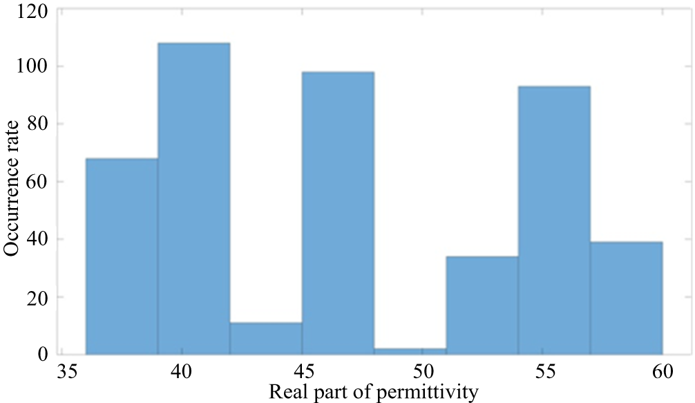
In the next step, the continuous images are discretized to extract the skull boundaries. To determine the optimal threshold, we used a histogram. Figure 7 shows the histogram for one of the top cross-sections (z = z 27). For better clarity, we present the estimated real part of the permittivity instead of the contrast. In the layers closest to the antennas (i.e., the top layers), the histograms consistently exhibit three distinct regions: one centered around 46, corresponding to soft tissue; another above 50, corresponding to brain tissue; and a third below 43, associated with the skull. Based on these observations, a threshold value of threshold (TH) = 44 is selected.
After binarizing the image using the threshold derived from the histograms, the external and internal skull boundaries are identified and then used to generate a skull model. Once the skull model is generated, the approximate head model is obtained by inserting the skull in the background model from Fig. 1 (b). The model comprises four distinct domains: (1) skull, (2) brain, (3) skin with fat, and (4) soft tissue occupying the remaining volume. The brain and skull regions were flattened at the depth corresponding to the effective field penetration, as the scattered fields originating from layers below this level were found to be negligible. The obtained phantom is presented in Fig. 8.
Typical histogram of the estimated real part of the permittivity in top layers (z = z 27).

Figure 7 Long description
A histogram showing the occurrence rate on the y-axis and the real part of permittivity on the x-axis, ranging from 35 to 60. The bars indicate varying occurrence rates across different permittivity values, with notable peaks around 40 and 55 and a lower occurrence near 45.
Geometry of the obtained patient-specific model with four tissues.

Figure 8 Long description
A 3D model depicting the layered structures of a head. The model includes distinct regions with different colors, representing various tissues or materials. The outermost layer is shown with a network of lines, possibly indicating a mesh structure. The inner layers are also represented with similar mesh patterns, each with unique shapes and boundaries. The model appears to illustrate the complexity of the head's anatomy or a similar structure.
DBIM results
In order to complete the patient-specific model, the permittivities of the four domains should be calculated. To that aim, the DBIM procedure described in the “DBIM formulation with known domain boundaries” subsection was employed. The same search space, comprising 34,947 voxels inside the head, was used as in the previous subsection. Once the DBIM was performed and the values of permittivities were obtained, the scattering matrix of the patient-specific model was calculated using WIPL-D Pro. To evaluate the accuracy of the approximation of the original six-domain model by the obtained model, the relative root mean square error (RRMSE) of the scattering parameters, denoted as δ, was computed:
 \begin{equation}\delta = \sqrt {\frac{{\sum\limits_{k = 1}^M {\sum\limits_{j = 1}^M {{{\left| {s_{kj}^{} - s_{kj}^{ref}} \right|}^2}} } }}{{\sum\limits_{k = 1}^M {\sum\limits_{j = 1}^M {{{\left| {s_{kj}^{ref}} \right|}^2}} } }}} \cdot 100{\text{ }}\% ,\end{equation}
where  ${s_{kj}}$ and $s_{kj}^{ref}$ are the scattering parameters calculated for the model obtained from the DBIM and the original model with six tissues (Fig. 1 (a)), respectively.
As the first test of the DBIM, we assumed the boundaries of the six-domain phantom from Fig. 1(a) were precisely known. The initial values of permittivity for all tissues were set to the average value (34.64–j12.68) from [Reference Singh, Ninkovic, Tasic, Stevanovic and Kolundzija24]. In this case, the DBIM converged to the permittivity actual values from Table 1 after five iterations.
Furthermore, to assess the maximal accuracy that can be obtained from the model with four tissues, two parametric models were created from the original model with six tissues, assuming that intertissue boundaries are known. Namely, the facial bones were removed from the skull, and the true skull boundaries were parameterized using spherical harmonics, up to two different cutting planes. As a result, parametric model 1 (Fig. 9(a)) and parametric model 2 (Fig. 9(b)) were obtained.
(a) Parametric model 1. (b) Parametric model 2.

Figure 9 Long description
The image shows two parametric models labeled as (a) and (b). Both models depict a cross-section of a skull with distinct layers. Model (a) features a visible cutout section, while model (b) shows a complete section. The models illustrate different parameterizations of tissue boundaries, with various colors representing different tissues. The outermost layer is marked with protruding elements, possibly indicating measurement points or structural features.
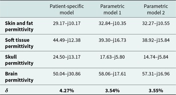
For both parametric models and the patient-specific model from Fig. 7, the DBIM converged within 10 iterations (7 iterations for the patient-specific model and 6 iterations for each of the parametric models). Each of the three WIPL-D models had around 33,000 unknowns, and thus each DBIM iteration lasted for about 50 min. The obtained values of permittivities and RRMSE are presented in Table 2.
DBIM results

Table 2 Long description
The table compares permittivity values for different tissues across a patient-specific model and two parametric models. The brain permittivity is highest in the patient-specific model at 50.04, compared to 58.06 and 57.31 in the parametric models. Skin and fat permittivity is lowest in the patient-specific model at 29.17, while parametric models show slightly higher values. Soft tissue permittivity is highest in the patient-specific model at 44.49, with parametric models showing lower values. Skull permittivity is significantly lower in parametric models compared to the patient-specific model. The delta values indicate the percentage difference, with the patient-specific model having the highest at 4.27 percent. These variations suggest differences in tissue characterization between the models.
When the exact skull boundaries were used for the parameterization, RRMSE values of 3.54% and 3.55% were achieved. On the other hand, for a patient-specific model created from the reconstructed permittivities, an RRMSE of 4.27% was attained. For comparison, the minimum RRMSE that could be obtained by approximating the original model with the homogenous head phantom was 12.27%. Thus, the patient-specific four-tissue model that used the same a priori information achieved almost three times lower value of error.
For the initial two-layer model used for the generation of the patient-specific model, the RRMSE was 26.3%. Equivalently, the signal-to-modeling-error power ratio improved from about 11 dB for the initial two-layer model to approximately 27.4 dB for the patient-specific model.
Moreover, the robustness of the DBIM with respect to measurement noise was evaluated by incorporating AWGN into the simulated scattering parameters of the original six-domain model. Noise levels corresponding to SNR values of 20, 15, and 10 dB were considered.
To isolate the effect of noise on the DBIM algorithm, independent of its impact on the construction of the four-domain phantom, the tissue geometry obtained under noiseless conditions was employed. The corresponding permittivity estimates and RRMSE values are reported in Table 3. In all cases, the DBIM algorithm converged within 10 iterations.
DBIM results for the patient-specific model with AWGN applied to the scattering parameters at different SNR levels

Table 3 Long description
The table measures permittivity values of different tissues at varying signal-to-noise ratio levels. Brain permittivity shows a notable increase from 41.79 at 15 dB to 62.25 at 10 dB, indicating a significant change as noise increases. Skin and fat permittivity slightly decreases from 31.11 at 15 dB to 29.44 at 10 dB. Soft tissue permittivity remains relatively stable across SNR levels, with minor fluctuations. Skull permittivity shows a marked increase at 10 dB compared to lower SNR levels. The percentage change, denoted as delta, increases from 4.30% at 20 dB to 6.25% at 10 dB, suggesting greater variability in permittivity measurements at lower SNR levels.
As shown in Table 3, reconstruction accuracy gradually decreases with decreasing SNR, reflecting the growing influence of noise. For SNR levels of 20 and 15 dB, the estimated permittivity values remain close to those obtained in the noiseless case, with only a moderate increase in RRMSE. Even at an SNR of 10 dB, the DBIM algorithm converges reliably, although deviations in the permittivity of inner tissues (such as the skull and brain) become more pronounced. These findings are consistent with the MWI results presented in Fig. 6, where an SNR of 10 dB relative to the total signal appears to represent a threshold beyond which more significant degradation occurs. Considering that stroke-related signals are more than 50 dB weaker than the total signal, it can be concluded that the examined noise levels are unlikely to significantly impact the primary application of the patient-specific background model.
Conclusion
This work has presented an advanced methodology for constructing patient-specific head models to enhance quantitative MMWI. The proposed framework integrates an anatomically conformal parameterization of the head geometry, obtained through a spherical harmonic approximation of the interpolated surface points. This approach ensures a geometrically consistent representation of the region of interest, particularly in the upper cranial portion, which is relevant in microwave measurements, and it provides a practical pathway for building individualized models directly from measured data.
The proposed method was assessed numerically, building upon a realistic six-tissue head phantom derived from the NEVA female anatomical model. The simulations were conducted in the WIPL-D Pro environment using a 21-antenna helmet array operating at 1 GHz. A linearized reconstruction was first applied to estimate the real part of the permittivity contrast, followed by histogram-based segmentation to delineate the skull boundaries and define four distinct tissue domains. The permittivity values of these tissues were then quantitatively estimated using the DBIM. The resulting patient-specific four-tissue model achieved a RRMSE of 4.27%, closely matching the 3.54% obtained using exact skull boundaries and significantly outperforming the homogeneous head approximation (12.27% RRMSE).
These results demonstrate that the proposed modeling strategy substantially improves the accuracy of DBIM, while maintaining computational efficiency. The capability to generate reliable individualized background models directly from microwave data represents a significant step toward enhancing the initialization and convergence of quantitative inverse scattering algorithms, thus advancing MMWI toward practical clinical implementation.
Acknowledgement
This work was supported in part by the Ministry of Science, Technological Development and Innovations of the Republic of Serbia, under Contract 451-03- 137/2025-03/200103.
Competing interests
The authors report no conflict of interest.

Darko Ninković was born in Belgrade, Serbia, in 1995. He received the BSc and MSc degrees in electrical engineering from the School of Electrical Engineering, University of Belgrade, in 2018 and 2019, respectively, where he is currently pursuing the PhD degree. His current research interests include microwave imaging, optimization algorithms and machine learning applied to the electromagnetic analysis, electromagnetic compatibility, and numerical electromagnetic analysis.

Anja Kovačević was born in Belgrade, Serbia, in 1999. She received the BSc and MSc degrees in electrical engineering from the School of Electrical Engineering, University of Belgrade, in 2022 and 2023, respectively, where she is currently pursuing the PhD degree. In 2022, she joined the School of Electrical Engineering, University of Belgrade, as a teaching associate and currently is a teaching assistant at the same school. Her current research interests include microwave imaging, microwave passive circuits and electromagnetic compatibility. She was a recipient of IEEE MTT-S Undergraduate Scholarships – 2023 Cycle 1 Award.

Branko Kolundžija was born in Zenica, former Yugoslavia, in 1958. He received the BSc, MSc, and DSc degrees from the University of Belgrade, Belgrade, Serbia, in 1981, 1986, and 1990, respectively. He joined the School of Electrical Engineering, University of Belgrade, in 1981, as an assistant-trainee, in 1986 as an assistant, in 1991 as an assistant professor, in 1998 as an associate professor and in 2003 as a full professor, teaching electromagnetics, antennas and propagation of radio waves, software tools for designing antennas, and modeling and simulation of electromagnetic fields. He is the author/coauthor of two monographs, five monograph chapters, three monographs accompanied by software packages, one textbook, more than 60 journal articles, and more than 200 articles at international conferences, in the areas of numerical and theoretical electromagnetics, antennas, microwave technique, electromagnetic compatibility, applied mathematics, and artificial intelligence. He is the main architect of the WIPL-D software suite.

Rosa Scapaticci received her master’s degree with honors in Biomedical Engineering from the University of Naples “Federico II” in 2010 and her PhD in Information Engineering from the “Mediterranea” University of Reggio Calabria in 2014. She is currently a senior researcher at the Institute for Electromagnetic Sensing of the Environment of the Italian National Research Council in Naples. Her research focuses on electromagnetic scattering and imaging techniques for noninvasive diagnostics, with particular emphasis on developing innovative microwave imaging approaches for biomedical applications. She received the Best Student Member Paper Award from the IEEE Antennas and Propagation Society in 2013, and the Barzilai and Latmiral Awards from the Italian Society of Electromagnetics in 2014 and 2018, respectively. In 2021, she obtained the National Scientific Qualification as Associate Professor in electromagnetic fields. From March 2022 to April 2026, she served as Associate Editor for IEEE Transactions on Medical Imaging.

Lorenzo Crocco is Research Director at the Institute for Electromagnetic Sensing of the Environment, National Research Council of Italy (IREA-CNR). His research focuses on electromagnetic scattering methods and applications, with particular emphasis on noninvasive diagnostics and therapeutic uses of electromagnetic fields. He has authored over 120 papers and edited two books. Since 2021, he has been listed in the World’s Top 2% Scientists database. He serves on the Scientific Board of the Italian Electromagnetic Society and the CNR Engineering Department Scientific Board. Since 2014, he has been a Board Member of the European School of Antennas (ESoA). Since 2024, he has represented Italy, San Marino, and Vatican City in the Delegate Assembly of the European Association on Antennas and Propagation (EurAAP). Within EurAAP, he also founded the Working Group on Electromagnetic Technologies for Life Science Applications (ELSA). Lorenzo Crocco is an IEEE Senior Member and URSI Senior Member.

Marija Nikolić Stevanović received the BSc, MSc, and PhD degrees in electrical engineering from the University of Belgrade, Serbia, in 2000, 2003, and 2007, respectively, and an additional PhD degree from Washington University in St. Louis, USA, in 2011. In 2011, she joined the School of Electrical Engineering at the University of Belgrade as a teaching assistant and was promoted as Full Professor in 2022. Her research interests include inverse scattering, microwave imaging, numerical electromagnetics, and antenna design. In recent years, her work has focused particularly on microwave medical imaging. She has served as the Serbian representative on the Management Committees of COST Actions dedicated to medical applications of electromagnetic fields, including MiMed (microwave imaging) and MyWAVE (therapeutic applications of electromagnetic waves). She also served as Vice-Dean for Research at the School of Electrical Engineering during 2024–2025.







 Open access

