


1. Introduction
Thermoacoustic instabilities in turbulent combustors are a recurring problem in gas turbines for aeronautic and power generation applications (Poinsot Reference Poinsot2017). Entropy waves, produced by the unsteady reacting flow and transported throughout the combustion chamber, can actively participate in the constructive feedback between the acoustic field and the flames (Morgans & Duran Reference Morgans and Duran2016). It is, therefore, crucial to understand their generation and transport and thus the dispersion and interaction of entropy waves with the downstream flow. Of particular interest is their interaction with the high-Mach regions at the turbine inlet, where their acceleration leads to the production of transmitted and reflected acoustic waves (Marble & Candel Reference Marble and Candel1977), and with the autoignition flames in sequential combustors (Weilenmann et al. Reference Weilenmann, Xiong, Bothien and Noiray2018). Indeed, the entropy-wave-induced acoustic oscillations coherently force the reactive flow in the combustor, which sustains the generation of entropy waves and thus closes the loop. It is seen as the key mechanism governing low-frequency thermoacoustic instabilities in aeroengines, often referred to as ‘rumble’. This study focuses on the dispersion of these entropy waves, which varies significantly from one combustor to another and which is key for the triggering of these low-frequency instabilities.
Our work follows a number of experimental and numerical investigations dealing with the generation of entropy waves (e.g. Wang et al. Reference Wang, Liu, Wang, Li and Qi2019; Yoon Reference Yoon2020), with their contribution to the instabilities (e.g. Eckstein & Sattelmayer Reference Eckstein and Sattelmayer2006; Schulz et al. Reference Schulz, Doll, Ebi, Droujko, Bourquard and Noiray2019) and with their measurements (Wassmer et al. Reference Wassmer, Schuermans, Paschereit and Moeck2017; De Domenico et al. Reference De Domenico, Shah, Lowe, Fan, Ewart, Williams and Hochgreb2019). Most of the modelling efforts to date have been about entropy-wave dispersion in fully developed turbulent duct flows (Sattelmayer Reference Sattelmayer2002; Morgans, Goh & Dahan Reference Morgans, Goh and Dahan2013; Morgans & Duran Reference Morgans and Duran2016; Giusti et al. Reference Giusti, Worth, Mastorakos and Dowling2017; Fattahi, Hosseinalipour & Karimi Reference Fattahi, Hosseinalipour and Karimi2017; Christodoulou et al. Reference Christodoulou, Karimi, Cammarano, Paul and Navarro-Martinez2020; Hosseinalipour et al. Reference Hosseinalipour, Fattahi, Khalili, Tootoonchian and Karimi2020), where shear dispersion was identified as the dominant mechanism. There are indeed several mechanisms at play that contribute to the decay of entropy waves (e.g. Polifke Reference Polifke2020), but molecular diffusion and turbulent mixing caused by homogeneous isotropic turbulence were found to be of minor importance. However, these canonical flows are much less complex than the flows in real engines, which motivated Xia et al. (Reference Xia, Duran, Morgans and Han2018) and Giusti & Mastorakos (Reference Giusti and Mastorakos2019) to perform a numerical study based on simulations of the flow in gas turbine combustors, from which they concluded that large-scale unsteady flow structures significantly influence the dispersion of entropy waves. However, experimental data are very scarce, particularly in harsher highly turbulent environments with large-scale coherent structures, such as swirl and jets from dilution holes. The present work aims to contribute toward filling this gap by providing measurements of coherent temperature fluctuations in a high-Reynolds-number duct flow ( $Re=140\,000$) in which entropy waves are generated using a pulsed hot jet. Because of this periodic injection process, large-scale coherent turbulent structures (e.g. Haller Reference Haller2015) are formed together with the entropy waves. The decay of these waves is quantified using high-speed background-oriented schlieren (BOS) thermometry with a methodology, which is explained in § 2. These experimental measurements are complemented with large eddy simulations (LES), whose numerical set-up is presented in § 3, and the results are presented and discussed in § 4.
2. Experimental set-up and data processing method
The experimental set-up, composed of a wind tunnel with constant rectangular cross-section and a siren for creating a pulsed hot jet in cold cross-flow, is shown in figure 1. The tunnel was operated at an absolute pressure of  $\bar {p}=1.3$ bar by throttling the inlet and the outlet of the test rig, resulting in a steady mass flow of $150\ \textrm {g}\,\textrm {s}^{-1}$, with a temperature of $315$ K in the test section. The duct has constant inner height and width, $H=57$ mm and $W=25$ mm, respectively, and top and side borosilicate windows for optical access in its central part. Entropy waves are generated by a siren upstream of the test section. The siren consists of a rotating perforated disk and an electric heater supplied with $20\ \textrm {g}\,\textrm {s}^{-1}$ of pressurized air as shown in figures 1(c) and 1(d). The frequency of this pulsed hot jet in cross-flow is controlled by adjusting the rotational speed of the disk. For this study, the pulsed-jet frequency $f$ is successively set to 240, 480, 720 and 900 Hz. For each frequency, five heater settings were tested, leading to siren air temperatures $T_j$ of 321, 367, 414, 469 and 519 K measured with a thermocouple placed just upstream of the siren disk. The test conditions result in mean bulk velocities in the duct between $70$ and $90\ \textrm {m}\,\textrm {s}^{-1}$. The temperature in the duct is broken up using the classic triple decomposition: $T(\boldsymbol {x},t)=\bar {T}(\boldsymbol {x})+\tilde {T}(\boldsymbol {x},t)+\check {T}(\boldsymbol {x},t)$, where $\bar {T}$ is the mean temperature, $\tilde {T}$ and $\check {T}$ are the zero mean coherent and turbulent components of the fluctuating temperature, $\langle T \rangle = \bar {T}+\tilde {T}$ the phase-averaged temperature and $T^\prime {}=\tilde {T}+\check {T}$ the zero mean fluctuations. This work aims to identify the coherent component $\tilde {T}(\boldsymbol {x},t)$ and characterize its spatio-temporal decay, since it is highly relevant for low-frequency thermoacoustic instabilities, involving entropy wave feedback. The characterization of $\tilde {T}(\boldsymbol {x},t)$ is achieved by combining high-speed BOS with particle image velocimetry (PIV). The latter is used to quantify the streamwise oscillating velocity which is needed for the data processing of the BOS results. Particle image velocimetry at 12.5 kHz is performed in the vertical central plane of the test section, with a high-speed camera positioned on its side and with a laser sheet passing through the top window as indicated in figure 1. The field of view (FOV) was adjusted to match the one of the BOS thermometry by using Scheimpflug optics. The camera was equipped with a Nikon AF 200 mm micro Nikkor lens and a 532 nm bandpass filter from Edmund Optics. A Photonics DM60 Nd:YAG was used to generate a pulsed 532 nm laser light sheet originating from a laser arm and sheet optics from Lavision. The mean temperatures of the main air flow upstream of the siren, of the heated-air pulsed jet and of the flow in the FOV are measured with thermocouples as indicated in figure 1. The acoustic pressure $\tilde {p}$ was recorded with a piezoelectric sensor type 211B5 from Kistler. The telecentric BOS set-up mounted on an optical rail is shown schematically in figure 1(a). It enables plane measurements of the line-of-sight (LOS) integrated refraction index gradient $\boldsymbol {\nabla }n(\boldsymbol {x},t)$, perpendicular to the optical axis, as in classical BOS (Raffel Reference Raffel2015). It is composed of a high-speed camera, a telecentric lens system (Ota et al. Reference Ota, Leopold, Noda and Maeno2015) and a background filled with randomly distributed dots illuminated with an LED. The telecentric lens system brings the advantage of increased depth of field, which minimizes the blur of the observed $\boldsymbol {\nabla }n(\boldsymbol {x},t)$ structures while keeping the background in focus (Ota et al. Reference Ota, Leopold, Noda and Maeno2015). Also, no scaling factors are required between the measurement plane and the background plane because the light can be assumed to be parallel to the optical axis. The LOS integrated $n$ field is obtained by solving the Poisson equation
 \begin{equation} \boldsymbol{\nabla}\boldsymbol{\cdot}\boldsymbol{\nabla} n(\boldsymbol{x},t) = \frac{n_0}{WZ_d} \boldsymbol{\nabla}\boldsymbol{\cdot} \boldsymbol{\delta}(\boldsymbol{x},t), \end{equation}
which is obtained by taking the divergence of the classical BOS equation (Raffel Reference Raffel2015). In this equation,  $\boldsymbol {\delta }$ is the displacement vector field obtained by applying a cross-correlation algorithm between images of the illuminated background pattern, $Z_d$ is the distance from the centre of the schlieren object to the background and $W$ is the thickness of the object (see figure 1). Traditionally, $\boldsymbol {\delta }(\boldsymbol {x},t)$ is obtained by correlating a reference image $I_{r}(\boldsymbol {x})$ without the entropy wave (before starting the experiment) and measurement images, providing intensity fields $I({\boldsymbol {x},t})$ once the desired test condition has been reached (Raffel Reference Raffel2015). The resulting $\boldsymbol {\delta }_{tot}(\boldsymbol {x},t)$ can be decomposed as
 \begin{equation} \boldsymbol{\delta}_{tot}(\boldsymbol{x},t) = \boldsymbol{\delta}_{fsd}(\boldsymbol{x},t)+\boldsymbol{\delta}_{ssd}(\boldsymbol{x})+\boldsymbol{\delta}_{path}(\boldsymbol{x})+\boldsymbol{\delta}_{e}(\boldsymbol{x},t), \end{equation}
where  $\boldsymbol {\delta }_{e}$ is the component of the total displacement field, which is induced by the presence of the schlieren object. The other components are spurious and optical-path-related displacements that have been recently investigated by Xiong, Weilenmann & Noiray (Reference Xiong, Weilenmann and Noiray2020). The components $\boldsymbol {\delta }_{fsd}$ and $\boldsymbol {\delta }_{ssd}$ are spurious displacements that are fast and slow with respect to the acquisition time of a high-speed imaging recording (in the present case, 0.4 s for 5000 frames recorded at 12.5 kHz). In our experimental set-up, the origin of $\boldsymbol {\delta }_{ssd}$ is attributed to the heating of the camera sensor between the acquisition of $I_{r}(\boldsymbol {x})$ and $I({\boldsymbol {x},t})$, while $\boldsymbol {\delta }_{fsd}$ results from the vibrations induced by the camera fan (Xiong et al. Reference Xiong, Weilenmann and Noiray2020). In (2.2), $\boldsymbol {\delta }_{path}$ is the displacement induced by temperature fluctuations along the optical path, which have here been reduced by thermally protecting this optical path. In the present experimental set-up, during one recording, $\boldsymbol {\delta }_{path}$ and $\boldsymbol {\delta }_{ssd}$ can be considered as steady with respect to the targeted displacement $\boldsymbol {\delta }_{e}$ that is induced by the fast travelling entropy waves in the duct. In order to remove these quasi-steady components of the spurious displacement, the reference field is replaced by the average of the measurement intensity fields $I_{r}=(1/N)\sum_{i=1}^{N}I(\boldsymbol{x},t_i)$, which is one of the strategies proposed by Xiong et al. (Reference Xiong, Weilenmann and Noiray2020), and which is particularly effective for the present set-up. Furthermore, the vibration-induced spurious displacement $\boldsymbol {\delta }_{fsd}$ is suppressed through the averaging in the stitching process described below.
(a) Top view of the experimental set-up including optical diagnostics. (b) Side view of the set-up. (c and d), respectively, show vertical and horizontal sections depicting the periodically pulsed hot air injection and the rotating disk.

The displacement fields  $\boldsymbol {\delta }_{e}(\boldsymbol {x},t)$ are proportional to the instantaneous LOS-integrated refraction index gradients produced by the passing entropy waves. They are used to deduce the coherent temperature fluctuations $\tilde {T}(\boldsymbol {x},t)$ by integrating the Poisson equation (2.1). However, this integration cannot be directly performed. This is because only a fraction of the convective wavelength $\lambda _c$ can be captured within the FOV of the camera. Consequently, one has to stitch the instantaneous fields together before integrating the Poisson equation, which we do using a new coordinate system $\boldsymbol {\chi }=(\chi , y)$. This allows us to position the instantaneous displacement fields with respect to each other within an entire wavelength $\lambda _c$. Indeed, the centre of each instantaneous displacement field is defined by the axial coordinate $\chi$, which takes into account the oscillating axial velocity, according to
 \begin{equation} \chi(\varphi)=\frac{1}{2{\rm \pi} f}\int_{0}^{\varphi}\langle u_x \rangle (\phi)\,\textrm{d}\phi, \end{equation}
where  $\varphi$ is the instantaneous phase (modulo $2 {\rm \pi}$) of the acoustic pressure signal at the forcing frequency $f$, and $\langle u_x \rangle$ is the phase-averaged axial velocity in the centre of the test section, obtained by PIV, an example of which is shown in figure 2(a). The BOS velocimetry data, also shown in figure 2(a), was obtained using the optical flow algorithm as described in Weilenmann et al. (Reference Weilenmann, Xiong, Bothien and Noiray2018). This approach represents an alternative way to quantify the needed velocity information if PIV is not available. When processing the case displayed in figure 2 with the BOS velocimetry data, the extracted entropy wave amplitude at the pulsed-jet frequency changes by 4.3 %. In the remainder of this work, the PIV data were used for all the processing because of its higher accuracy. This stitching process is illustrated in figures 2(b) and 2(c), and once all the instantaneous displacement fields are placed in this coordinate system, their averaging is performed to obtain the coherent component of the displacement field $\boldsymbol {\delta }_{e}(\boldsymbol {\chi })$. Considering that one may argue that non-negligible decay of the entropy wave could happen in the streamwise direction within the BOS FOV, the instantaneous fields $\boldsymbol {\delta }_{e}(\boldsymbol {x},t)$ were systematically cropped to 10 % of $\lambda _c$ before proceeding with the stitching process. This cropping ensures a robust reconstruction of the coherent displacement field, an example of which is given in figure 2(d) for $f=240$ Hz, $T_j= 519$ K and with $96$ cycles used for the averaging. For all frequencies considered in this work, the extracted entropy wave amplitude converged after including 40 cycles in the stitching process to a value within ${\pm }5\,\%$ of the amplitude obtained by stitching 90 cycles. It is important to mention that the coordinate $\chi$ allows us to spatially represent the entropy waves at a given axial location, as if their amplitude decay had been frozen from that point.
(a) Phase-averaged velocity  $\langle u_x \rangle$ from PIV data. (b) Instantaneous displacement fields $\boldsymbol {\delta }_{e}(\boldsymbol {x},t)$. (c) The instantaneous snapshots are placed within a panorama, using (2.3). In the overlapping areas, the displacement fields are averaged. The convective wavelength $\lambda_c$ is the ratio of the mean bulk velocity $\bar{u}$ to the pulsed-jet frequency $f$. (d) Resulting phase-averaged displacement field $\tilde {\boldsymbol {\delta }}_{e}(\boldsymbol {\chi })$ representing one acoustic cycle (here $f=240\,{\rm Hz}$ and $T_j=519$ K).

Since no spatial stretching is applied, (2.1) can also be applied in the new coordinate system  $\boldsymbol {\chi }$, and it can be integrated using a Poisson solver to obtain the coherent refraction index field $\tilde {n}$ from the coherent displacement field $\boldsymbol {\tilde {\delta }}_{e}$. To achieve BOS thermometry, $n$ is converted to $T$ via the Gladstone–Dale relation $\rho ={n-1}/{G}$ and the ideal gas law $\bar {p} = \rho RT$, where $\rho$ is the density, $G$ the Gladstone–Dale constant, $R$ the gas constant of air and $\bar {p}$ the static pressure in the duct. A K-type thermocouple placed in the centre of the FOV provides the mean temperature, which is assumed to be uniformly distributed in the duct and which is used as the integration constant for performing quantitative extraction of the coherent temperature fluctuations.
Since the described processing only requires mean quantities as inputs, it is suitable for high-frequency entropy wave measurements in very fast flows. The main limitation is the camera exposure time, which has to be short enough to capture the passing gradient structures while still allowing enough light to reach the sensor. By applying this post-processing of the BOS and PIV data, as is done in § 4, one can extract  $\tilde {T}(\boldsymbol {\chi })$, which is the LOS-integrated coherent part of the temperature fluctuations in the camera FOV.
3. Numerical set-up
Large eddy simulations of the pulsed hot jet in cross-flow are performed using the explicit solver AVBP (e.g. Gicquel et al. Reference Gicquel, Gourdain, Boussuge, Deniau, Staffelbach, Wolf and Poinsot2011) for several temperatures of the 720 Hz pulsed jet and for the same average mass flows as in the experiments. A cut through the computational domain is shown in figure 3(a). A constant cross-section transition piece connects the outlet of the round cross-section convergent present in the experiment to the wind tunnel of rectangular cross-section  $HW$. This convergent was included in the simulation domain in order to reproduce the development of the boundary layer upstream of the siren inlet. The plenum and its acoustic absorbing material, just upstream of the convergent, and the downstream divergent and sound absorber were not simulated, but their effect on the acoustics of the system at 720 Hz were accounted for with non-reflecting boundary conditions as explained below. The cell sizes in the duct are sufficiently small to resolve a minimum of 80 % of the turbulent kinetic energy. The mesh in the convergent is much coarser, while the region of the hot jet-in-cross-flow is further refined as shown in figure 3. Overall, 24 million tetrahedral cells are used, with non-reflective boundary conditions at the main inlet and at the outlet of the domain, while the pulsed hot jet-in-cross-flow is generated with a stiff inlet condition, the bulk velocity of which is shown in figure 3(a). Relaxation coefficients $K$ at the inlet and outlet are, respectively, set to 3000 and $1000\ \textrm {s}^{-1}$, which corresponds to cutoff frequencies $f_c=K/4{\rm \pi}$ of 80 and 240 Hz (Selle, Nicoud & Poinsot Reference Selle, Nicoud and Poinsot2004) that are well below the pulsed-jet frequency, and which prevents the reflection of acoustic waves at these boundaries. The subgrid-scale Reynolds stresses are modelled using the classic Smagorinsky approach and an adiabatic law of the wall is prescribed. The present use of the second-order Lax–Wendroff numerical scheme was validated for one of the simulations by comparing it to a more computationally expensive simulation with a two-step Taylor–Galerkin scheme that gives third-order accuracy in space and time. Figure 3(c) shows temperature isocontours from the simulation of the pulsed jet with its inlet temperature set to $T_j=469$ K.
(a) Cut through the unstructured tetrahedral LES mesh, and imposed bulk velocity at the inlet of the pulsed hot jet-in-cross-flow versus time. The velocity inlet in the LES was set in order to match the siren mass flow rate measured in the experiments. (b) Magnification of the mesh cut at the siren injection. (c) Isocontours of dispersing entropy waves at  $720$ Hz.

4. Experimental and numerical results
First, the non-intrusive experimental method proposed in § 2 allows us to quantify coherent LOS-integrated temperature fluctuations as low as 0.1 % of the mean flow temperature. This achievement is illustrated in figure 4, which shows  $\tilde {T}(\boldsymbol {\chi })$ for pulsed-jet frequencies of $240$ Hz and $480$ Hz and for several pulsed-jet temperatures
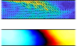
  $T_j$. The stitching and averaging process described in § 2, is also applied to the Mie scattering images of the seeded flow. Since only the tunnel flow is subject to particle seeding, one can qualitatively identify the entropy waves from the intensity of this Mie scattering signal, assuming thermal diffusion is not dominant (Giusti et al. Reference Giusti, Worth, Mastorakos and Dowling2017). Low and high luminosity, respectively, correspond to hot and cold regions. The results presented in figures 4(b) and 4(d) are in close agreement with the BOS results. For increasing jet temperature, the location of the entropy wave minimum slightly shifts in the downstream direction. This can be attributed to the slightly higher velocities at increased jet temperatures, which change the phase difference between the acoustic pressure signal and the entropy wave passing through the FOV of the BOS camera. Furthermore, the change in field size between figures 4(a) and 4(c) results from the change in convective wavelength $\lambda _c$.
Panels (a and c), respectively, show  $\tilde {T}(\boldsymbol {\chi })$ for pulsed-jet frequency of $240$ and $480\,{\rm Hz}$. From top to bottom, the jet exit temperature $T_j$ is set to $321$, $367$, $414$, $469$ and $519\,{\rm K}$. Panels (b and d) show the corresponding phase-averaged Mie scattering intensity.

Second, the LES provide complementary information on these complex flows as illustrated in figures 5(a) and 5(b), which show the decaying temperature and velocity waves in the central plane of the simulated domain for  $T_j=469$ K. The pulsed hot jet does not only generate entropy waves but also acoustic waves which are travelling up and downstream from the injection point. These acoustic waves are visible in figure 5(c) with amplitudes that can reach several thousand pascals, in agreement with the experimental measurements.
Temperature (a), axial velocity (b) and total pressure (c) in the central plane of the computational domain. The markers in (b) indicate the streamwise locations (3 cm upstream and 2 cm downstream of the jet) used for the extraction of the velocity field shown in figure 7.

In figure 6, experiments and LES are compared with regard to the rate at which the entropy waves decay for ranges of amplitudes and frequencies. For that purpose, the instantaneous 3-D temperature fields from LES were (i) spatially averaged at each axial location  $x$ in the $z$ and in the $y$ directions, and (ii) temporally phase-averaged during several simulated cycles, in order to obtain the streamwise decay of the coherent temperature fluctuations $\tilde {T}$ at the fundamental frequency. This post-processing is illustrated in figure 6(a), which shows $\tilde {T}(x=0.1 \ \text {m}, t)$, its power spectral density (PSD) and its fundamental component for $T_j=514$ K. Similarly, the experimental $\tilde {T}(\boldsymbol {\chi })$ are averaged in the $y$ direction and their Fourier amplitudes are deduced for each pulsed-jet frequency and temperature. The propagation and dispersion of entropy waves has shown to adhere well to the local Strouhal number $St= f L /\bar {u}$ in the experimental campaign by Wassmer et al. (Reference Wassmer, Schuermans, Paschereit and Moeck2017). Assuming the same is true for the current experiment, the comparison between experiments and simulations is performed by plotting the amplitudes of these coherent temperature fluctuations as a function of $St$, which is done in figure 6(b). For the simulations, $L$ varies and it is the axial distance from the jet to downstream distance of interest, while $\bar {u}$ and $f$ are fixed. For the experiments, $f$ varies and is defined by the siren, while $\bar {u}$ is nearly constant and $L$ is fixed and corresponds to the distance between the jet and the FOV. The validity of this approach is supported by the almost constant momentum ratio between jet and main stream for a fixed $T_j$. The amplitude decays of the simulated entropy waves are in close agreement with the low-Strouhal experimental dataset obtained for $f=240$ Hz. For higher $St$, the experimentally measured coherent fluctuations are smaller than the ones deduced from the LES, which can be explained by three reasons. Firstly, the LES is performed with adiabatic walls, while in the experiment convective heat transfer occurs at the walls. One can, for instance, refer to the paper from Rodrigues, Busseti & Hochgreb (Reference Rodrigues, Busseti and Hochgreb2019) who investigated the significant enhancement of the decay due to wall heat losses. Secondly, despite the fact that the experimental and simulation results scale very well with the local Strouhal number for $St<2$, this Strouhal scaling is maybe not the only governing non-dimensional number for higher $St$. Nevertheless, due to the complexity of the flow, conjecturing other scaling could not be easily validated, so it is not attempted in this work. Thirdly, the curves $\tilde {T}(St)$ deduced from the LES exhibit several local maxima, which correspond to the interferences between acoustically induced and entropy-wave-induced temperature fluctuations ( $\tilde {T}_a$ and $\tilde {T}_e$, respectively), and which cannot be captured by BOS thermometry, as the following content explains further. Indeed, the oscillating mass flow of the pulsed jet induces high-amplitude acoustic waves and the local temperature fluctuation $\tilde {T}$ can be decomposed as
 \begin{equation} \frac{\tilde{T}}{\bar{T}}=\frac{\gamma - 1}{\gamma}\frac{\tilde{p}}{\bar{p}}+ \frac{\tilde{s}}{c_p}, \end{equation}
where  $\gamma$ is the ratio of specific heats, $\tilde {s}$ the coherent fluctuations of the entropy and $c_p$ the specific heat at constant pressure. The first right-hand side term is $\tilde {T}_a/\bar {T}$ and the second is $\tilde {T}_e/\bar {T}$. These two contributions oscillate at the same frequency, but propagate at different velocities. While $\tilde {T}_e$ monotonically decays with $x$,
$x$,  $\tilde {T}_a$ is not significantly attenuated along the duct and dominates $\tilde {T}_e$ beyond a certain distance from the pulsed hot jet. In the simulated case, where $T_j=514\ \textrm {K}$, the amplitude of the plane acoustic wave downstream of the siren inlet is around $\tilde {p}\approx 4000$ Pa, which theoretically leads to $\tilde {T}_a\approx 3$ K, according to the first right-hand side term in (4.1). This agrees well with the amplitude of the local maxima observed in figure 6(b). The separation between the local maxima in $\tilde {T}$, which results from the interference between $\tilde {T}_e$ and $\tilde {T}_a$, is equal to $\lambda_b=\lambda_c(1+\bar{u}/c)$. This is the distance an acoustic wave has to travel to overtake a slower travelling entropy wave, with $\lambda _{c}$ being the convective wavelength of the entropy waves. The phase response of the entropy waves, which is not shown here, can simply be deduced from the convective velocity of the bulk flow, except in the vicinity of the jet because of the initial slowdown of the hot pockets due to the injection in cross-flow.
(a) Time trace of the cross-section-averaged temperature fluctuations at  $0.1$ m downstream of the jet for the simulation with $T_j=514$ K and $f=720$ Hz. The dashed line is the Fourier component at the pulsed-jet frequency $f$. (b) Fourier coefficient amplitudes from LES and experiments as a function of $St$. For the experimental data, the markers and their colours, respectively, define $f$ and $T_j$. (c) Rate of change of $\tilde {T}$ with respect to $St$, as function of $\tilde {T}$.

Furthermore, Christodoulou et al. (Reference Christodoulou, Karimi, Cammarano, Paul and Navarro-Martinez2020) found that for  $\tilde {T}/\bar {T}$ greater than $2\,\%$, the temperature waves start affecting the hydrodynamics of an established straight-duct turbulent flow, and cannot be treated as a passive scalar. These large amplitudes are observed in the present situation in the vicinity of the jet. In figure 6(c), the derivative of $\tilde {T}/\bar {T}$, with respect to the local Strouhal number $St$, is shown for two simulations in a similar way as in the paper of Christodoulou et al. (Reference Christodoulou, Karimi, Cammarano, Paul and Navarro-Martinez2020). A much faster decay rate is observed for $\tilde {T}/\bar {T} >0.04$ and $0.06$, respectively, which is, in the present situation, related not only to the large $\tilde {T}$, but also to the enhanced mixing from the coherent structures of the pulsed jet. Moreover, the loops in figure 6(c) correspond to the interference between acoustically induced and entropy-induced temperature fluctuations.
As mentioned earlier, even with more experimental data, i.e. closely spaced pulsed-jet frequencies, it was not possible to replicate the non-monotonous decay with the BOS thermometry approach proposed in § 2. Indeed, the averaged displacement fields resulting from the stitching process described in figure 2 only contain the perturbations travelling at the flow velocity in the duct and the perturbations propagating at the speed of sound are, therefore, eliminated though the averaging process. To illustrate this effect, the LES results for  $T_j=514$ K were processed in the same way as the experimental data and were plotted in figure 7(a) as $\tilde {T}_1$. Since the acoustic wavelength is much longer than the convective one, one has $\tilde {T}_1\approx \tilde {T}_e$. Adding the acoustic-induced temperature fluctuations $\tilde {T}_{a}$ based on the acoustic amplitudes of the forward travelling acoustic wave, one obtains $\tilde {T}_2$, which reproduces quite closely the local maxima observed in the direct extraction of the coherent fluctuations of the temperature $\tilde {T}_3$.
Processing of LES data for  $T_j=514$ K and $f=720$ Hz. (a) $\tilde {T}_1$, same processing as for the experimental data; $\tilde {T}_2$, superposition of $\tilde {T}_1$ and acoustically induced $\tilde {T}_a$; $\tilde {T}_3$, cross-section averaged coherent temperature fluctuation amplitudes; $\tilde {T}_4$, expected decay based on the $\bar {u}_x$ profiles (LES) shown in (b) for $x=-0.03$ m and in (c) for $x=0.02$ m. The dotted red lines indicate the $\lambda _b$ corresponding to the test conditions.

Finally, it is interesting to investigate the decay rate found in the present work and compare it to the model in Giusti et al. (Reference Giusti, Worth, Mastorakos and Dowling2017). This previous research showed that the decay of entropy waves in established turbulent duct flows can be reliably predicted by assuming that the shear dispersion is dominated by the radial profile of the mean axial velocity  $\bar {u}_x(0,y,z)$. For a rectangular cross-section in Cartesian coordinates, their model is
 \begin{equation} \frac{\tilde{T}(x)}{\tilde{T}_0}=\left|\frac{\iint_{\mathcal{A}} \bar{\rho}\,\bar{u}_x(y,z)\exp\left({-\textrm{i} \dfrac{2{\rm \pi} f x}{\bar{u}_x(y,z)}}\right)\textrm{d}y\,\textrm{d}z}{\iint_{\mathcal{A}} \bar{\rho}\,\bar{u}_x(y,z)\,\textrm{d}y\,\textrm{d}z}\right|, \end{equation}
where  $\tilde {T}_0$ is the amplitude at $x=0$ and $\mathcal {A}$ the cross-section area. The predictions $\tilde {T}_{4b}$ and $\tilde {T}_{4c}$ in figure 7(a) were obtained based on this model using the $\bar {u}_x$ profiles shown in figures 7(b) and 7(c). The use of the velocity profile of figure 7(b), extracted $30$ mm upstream of the jet, results in a very slow decay due to the absence of strong velocity gradients. Furthermore, the use of the profile in figure 7(c), which is extracted $20$ mm downstream of the jet, yields a faster decay, but it is still significantly underestimated compared to the actual decay $\tilde {T}_3(x)$. The present configuration better reflects the complexity of practical configurations than idealized numerical experiments based on pure entropy waves propagating in established straight-duct turbulent flows. This research showed that the decay of coherent entropy waves cannot be reliably predicted with this type of low-order model if only shear dispersion with a constant velocity profile is considered. Indeed, the dispersion is strongly enhanced by large-scale coherent turbulent structures and small-scale turbulence may also play a role in this enhancement. Nonetheless, properly accounting for the streamwise varying dispersion that is associated with the dynamics of these three-dimensional turbulent coherent structures will require development of more complex models (e.g. Steinbacher, Meindl & Polifke Reference Steinbacher, Meindl and Polifke2018) that may no longer be labelled as low-order models.
5. Conclusion
Entropy waves were generated with a pulsed hot jet in a highly turbulent cross-flow at frequencies up to 900 Hz. They were measured for amplitudes as low as 0.1 % of the mean temperature using BOS and simulated with LES, unravelling the fact that acoustic-wave-induced temperature fluctuations take precedence over ones resulting from the entropy waves beyond a critical Strouhal number. The complex, highly turbulent flow studied in this work leads to decays of coherent temperature fluctuations that are significantly faster than the ones predicted by models that are based on the assumptions that shear dispersion is mainly due to the profile of the mean axial velocity, and stays constant in the streamwise direction. Considering that practical turbulent combustors usually feature swirling flows with multiple dilution air streams, this work provides new data to support the development of models for entropy wave decay, and highlights the crucial need of models that account for dispersion effects due to coherent turbulent structures.
Declaration of interests
The authors report no conflict of interest.


 Open access