





1. Introduction
Reduced-order modelling techniques have been developed over several decades to capture coherent structures in fluid flows. These methods offer low-dimensional representations of the complex dynamics of fluid motion and serve as important tools to accelerate numerical prediction and flow control (Holmes et al. Reference Holmes, Lumey, Berkooz and Rowley2012; Rowley & Dawson Reference Rowley and Dawson2017). A prevalent approach to building a reduced-order model (ROM) involves projection methods, in which the velocity field is expanded into a finite set of test basis functions with unknown amplitude coefficients to be determined by solving the ROM. The residual of the governing equations is then made orthogonal to a set of trial functions using a space-only inner product, leading to the Galerkin (Rowley, Colonius & Murray Reference Rowley, Colonius and Murray2004) or Petrov–Galerkin methods (Carlberg, Bou-Mosleh & Farhat Reference Carlberg, Bou-Mosleh and Farhat2011). Various modal analysis methods have been employed to generate the basis functions, such as proper orthogonal decomposition (POD), balanced truncation or linear stability modes (see the review of Taira et al. (Reference Taira, Brunton, Dawson, Rowley, Colonius, McKeon, Schmidt, Gordeyev, Theofilis and Ukeiley2017)). The projection operation reduces the high spatial dimensionality of the original problem and yields a ROM in the form of a set of ordinary differential equations (ODEs).
This space-only modelling framework is particularly effective when the analysis at hand can be recast into the solution of an initial value problem, where the ROM is integrated forward in time from a known initial condition at reduced computational cost compared with the full-order system. Applications include the control of flow instabilities in transitional boundary layers (Semeraro et al. Reference Semeraro, Bagheri, Brandt and Henningson2011) and cavity flows (Barbagallo, Sipp & Schmid Reference Barbagallo, Sipp and Schmid2009), the suppression of turbulence in wall-bounded flows (Maia & Cavalieri Reference Maia and Cavalieri2025) and the modelling of the transient development of a bluff body wake (Noack et al. Reference Noack, Afanasiev, Morzyński, Tadmor and Thiele2003) and its control (Bergmann, Cordier & Brancher Reference Bergmann, Cordier and Brancher2005). However, many fluid mechanics problems are better framed through the analysis of the statistical properties of the fully developed turbulent state, i.e. the statistically stationary state reached when the flow settles onto a chaotic attractor. Such cases include the determination of bounds on time-averaged quantities (Chernyshenko et al. Reference Chernyshenko, Goulart, Huang and Papachristodoulou2014), the development of feedback control strategies for chaotic attractors (Tadmor et al. Reference Tadmor, Lehmann, Noack, Cordier, Delville, Bonnet and Morzyński2011; Lasagna et al. Reference Lasagna, Huang, Tutty and Chernyshenko2016; Leclercq et al. Reference Leclercq, Demourant, Poussot-Vassal and Sipp2019) and the characterisation of intermodal energy transfers (Couplet, Basdevant & Sagaut Reference Couplet, Basdevant and Sagaut2005; Rubini, Lasagna & Da Ronch Reference Rubini, Lasagna and Da Ronch2020; Jin, Symon & Illingworth Reference Jin, Symon and Illingworth2021).
In such circumstances, space-only ROMs may be inadequate. Firstly, the long-term boundedness of trajectories of a projection-based ROM, and therefore their statistical properties, is challenging to establish (Schlegel & Noack Reference Schlegel and Noack2015) or enforce when data-driven model identification methods are used (Kaptanoglu et al. Reference Kaptanoglu, Callaham, Aravkin, Hansen and Brunton2021; Peng et al. Reference Peng, Kaptanoglu, Hansen, Stevens-Haas, Manohar and Brunton2025). Second, these ROMs also unnecessarily retain most of the temporal dimensionality of the original problem, as numerical integration captures a wide range of temporal scales (Choi & Carlberg Reference Choi and Carlberg2019; Towne Reference Towne2021; Frame & Towne Reference Frame and Towne2024). Third, space-only ROMs exhibit spurious temporal modes, such as exponentially growing or decaying behaviour, which do not pertain to the developed state once the system has settled onto the attractor (Sharma, Mezić & McKeon Reference Sharma, Mezić and McKeon2016). Furthermore, closure models (Ahmed et al. Reference Ahmed, Pawar, San, Rasheed, Iliescu and Noack2021) or calibration techniques (Loiseau & Brunton Reference Loiseau and Brunton2018; Rubini et al. Reference Rubini, Lasagna and Da Ronch2020; Khoo, Chan & Hwang Reference Khoo, Chan and Hwang2022) are typically required to compensate for the influence of truncated modes on the ROM, particularly in high-Reynolds-number flows, yet constructing such corrections remains a significant obstacle.
1.1. The space–time ROM formalism
To address these limitations, space–time ROMs have been proposed (Yano Reference Yano2014; Choi & Carlberg Reference Choi and Carlberg2019). In these approaches, the solution is expanded into a set of space–time basis functions and the unknown amplitude coefficients are determined using different techniques from the solution of a linear or nonlinear algebraic problem, depending on the nature of the starting set of partial differential equations. Unlike space-only ROMs, space–time ROMs directly approximate the complete spatio-temporal trajectory of the system over a predetermined time period, without requiring temporal integration. Therefore, the desired temporal behaviour and resolution can be controlled a priori by a suitable choice of the temporal basis. Choi & Carlberg (Reference Choi and Carlberg2019) introduced a space–time least-squares Petrov-Galerkin method for nonlinear dynamical systems and applied it to one-dimensional nonlinear advection equations, demonstrating that error bounds grow subquadratically in time, as opposed to the exponential growth typical of space-only ROMs. Applications in optimal control (Baumann, Benner & Heiland Reference Baumann, Benner and Heiland2018) and haemodynamics (Tenderini, Mueller & Deparis Reference Tenderini, Mueller and Deparis2024) further illustrate the potential of this approach.
In the fluid mechanics community, efforts to construct space–time ROMs have only recently begun to emerge (Towne Reference Towne2021; Frame & Towne Reference Frame and Towne2024; Frame et al. Reference Frame, Lin, Schmidt and Towne2024; Li & Lasagna Reference Li and Lasagna2024) using resolvent modes (Jovanović & Bamieh Reference Jovanović and Bamieh2005; McKeon & Sharma Reference McKeon and Sharma2010; Sipp et al. Reference Sipp, Marquet, Meliga and Barbagallo2010) or spectral POD (SPOD) (Picard & Delville Reference Picard and Delville2000; Towne, Schmidt & Colonius Reference Towne, Schmidt and Colonius2018). Towne (Reference Towne2021) utilised these two bases in Galerkin and Petrov–Galerkin approaches, and found that space–time SPOD Petrov–Galerkin ROMs can produce accurate solutions with low computational cost in a one-dimensional (1-D) linearised Ginzburg–Landau problem. In Frame et al. (Reference Frame, Lin, Schmidt and Towne2024), applications to a 1-D linearised Ginzburg–Landau problem and a 2-D linear advection–diffusion problem have shown error reductions by several orders of magnitude compared with space-only methods, e.g. POD–Galerkin and balanced truncation, along with improved computational efficiency. Similar conclusions were reported in a subsequent study by Frame & Towne (Reference Frame and Towne2024), where the approach was extended to 1-D nonlinear Ginzburg–Landau systems that incorporate standard cubic and Burgers-type nonlinearities, using an iterative fixed-point technique to solve the resulting nonlinear algebraic system governing the amplitude coefficients of the space–time expansion. As noted in Frame & Towne (Reference Frame and Towne2024), this method may not always converge robustly, particularly under conditions of strong nonlinearity, although the circumstances influencing convergence remain to be fully understood and may vary with problem characteristics, especially in high-Reynolds-number flow regimes.
1.2. Relation with harmonic balance methods and unstable periodic orbits
When formulated using a Fourier basis in time, the case of resolvent and SPOD modes, space–time modelling techniques are closely related to harmonic balance (He & Ning Reference He and Ning1998; Hall et al. Reference Hall, Thomas and Clark2002, Reference Hall, Ekici, Thomas and Dowell2013). These methods have been popular in the turbomachinery community, where the temporal periodicity is inherent in the rotation of the system under study, but have also been applied more recently to transitional boundary layer flows (Rigas, Sipp & Colonius Reference Rigas, Sipp and Colonius2021), where this is not the case, and to capture limit cycle oscillations at moderate Reynolds numbers (Sierra-Ausin et al. Reference Sierra-Ausin, Citro, Giannetti and Fabre2022), where the oscillation period is obtained from the solution process. In these works, a system of nonlinear algebraic equations containing the unknown Fourier components of the time-periodic velocity field is derived and solved using root-finding techniques. Space–time modelling methods take a further step by expanding each Fourier component into a set of orthonormal spatial basis functions weighted by unknown amplitude coefficients, to reduce the dimensionality of the problem and achieve computational savings by solving a smaller system of algebraic equations.
For turbulent flows with a chaotic dynamics, a continuous spectrum and lacking strong periodic behaviour, the use of a temporal Fourier basis may still be justified in the limit of infinite time periods by the temporal homogeneity of flow statistics, akin to a large periodic spatial domain being used to approximate flows with spatial translational invariance (e.g. channels or pipes) (Sharma et al. Reference Sharma, Mezić and McKeon2016). This constitutes the most natural function space in which to describe the dynamics once the system has settled onto its attractor. More importantly, for finite (but unknown) time periods, the Fourier basis is still justified as it is the natural representation of unstable periodic orbits (UPOs), i.e. time-periodic exact solutions of the Navier–Stokes equations (see Kawahara, Uhlmann & van Veen (Reference Kawahara, Uhlmann and van Veen2012) and Graham & Floryan (Reference Graham and Floryan2021) for reviews). This property has motivated recent developments in UPO search methods (Parker & Schneider Reference Parker and Schneider2022; Burton et al. Reference Burton, Symon and Lasagna2025a ), which utilise a Fourier-in-time representation of the time-periodic velocity field.
The relationship between UPOs and the dynamical system theory viewpoint of turbulence needs to be further discussed. In principle, detailed knowledge of the hierarchy of short-period UPOs is sufficient to estimate infinite-time averages using cycle expansion theory (Artuso, Aurell & Cvitanovic Reference Artuso, Aurell and Cvitanovic1990). However, locating UPOs in fluid systems is challenging (Page et al. Reference Page, Norgaard, Brenner and Kerswell2024), posing hurdles to the application of cycle expansion theory to turbulence (Chandler & Kerswell Reference Chandler and Kerswell2013; Yalnlz, Hof & Budanur Reference Yalnlz, Hof and Budanur2021; Wang et al. Reference Wang, Ayats, Deguchi, Meseguer and Mellibovsky2025). This issue is relevant since the quality of cycle expansion theory predictions using an incomplete hierarchy of UPOs is as good as the most important orbit that one fails to locate (Budanur et al. Reference Budanur, Cvitanović, Davidchack and Siminos2015). In light of such issues, previous work (Lasagna Reference Lasagna2020) proposed a heuristic approach whereby available computational resources are spent to locate one or a few UPOs having a sufficiently long period $T$
. Using low-dimensional systems, such as the Lorenz equations, it was shown that time-averaged quantities and probability distributions computed on such UPOs appear to converge to those computed from chaotic trajectories as
$T$
. Using low-dimensional systems, such as the Lorenz equations, it was shown that time-averaged quantities and probability distributions computed on such UPOs appear to converge to those computed from chaotic trajectories as $T$
increases. This is intuitively justified by the fact that these orbits span the invariant measure of the chaotic attractor and provide a scaffold for chaotic trajectories to develop. More importantly for the purpose of this work, it was also shown that long UPOs provide access, via a well-behaved continuation analysis, to the sensitivity of time-averaged quantities with respect to problem parameters (Lasagna Reference Lasagna2018), as the periodicity effectively suppresses the exponential growth of the adjoint field (Wang Reference Wang2013), which makes classical adjoint sensitivity methods fail for chaotic systems (Lea, Allen & Haine Reference Lea, Allen and Haine2000). Understanding how the statistics of a turbulent flow depend on problem parameters (such as feedback control gains, geometry, wall attributes, design parameters, etc.) may be a key enabler to develop novel turbulence control strategies, but this information is hardly accessible in practice.
$T$
increases. This is intuitively justified by the fact that these orbits span the invariant measure of the chaotic attractor and provide a scaffold for chaotic trajectories to develop. More importantly for the purpose of this work, it was also shown that long UPOs provide access, via a well-behaved continuation analysis, to the sensitivity of time-averaged quantities with respect to problem parameters (Lasagna Reference Lasagna2018), as the periodicity effectively suppresses the exponential growth of the adjoint field (Wang Reference Wang2013), which makes classical adjoint sensitivity methods fail for chaotic systems (Lea, Allen & Haine Reference Lea, Allen and Haine2000). Understanding how the statistics of a turbulent flow depend on problem parameters (such as feedback control gains, geometry, wall attributes, design parameters, etc.) may be a key enabler to develop novel turbulence control strategies, but this information is hardly accessible in practice.
1.3. Motivation of the present study and main contributions
The tight mathematical and algorithmic connections between UPOs and space–time ROMs indicate that the latter may offer several opportunities to overcome the difficulties in computing long-period UPOs. Specifically, solutions of a space–time ROM may be interpreted as candidate approximations of UPOs of the full governing equations and thus may provide reduced-cost approximations of the long-time statistics of turbulent quantities pertaining to the full-order system. Then, when control and design parameters appear directly in the ROM, a numerical continuation study on ROM solutions, or using adjoint sensitivity methods, may shed light on how these statistics depend on such parameters. The adjoint sensitivity problem would be formulated directly within the reduced subspace as in Karbasian & Vermeire (Reference Karbasian and Vermeire2022), rather than in the complete state space, as in Sierra et al. (Reference Sierra, Jolivet, Giannetti and Citro2021), further reducing computational costs. Nevertheless, there are several fundamental hurdles in this programme of work that need addressing before this framework could be utilised for flow control and optimisation. We name a few key ones. First, nonlinear space–time methods need to be applied to fluid systems governed by the Navier–Stokes equations. Second, the relation between time-periodic solutions of a ROM and UPOs needs to be investigated in depth. Advances on this front have already been made (McCormack, Cavalieri & Hwang Reference McCormack, Cavalieri and Hwang2024). Third, for sensitivity analysis, the space–time basis needs to be sufficiently rich to capture a potentially complex parametric dependence, although progress may be made by leveraging model order reduction methods designed for time-periodic fluid systems, as in Padovan & Rowley (Reference Padovan and Rowley2024).
In this paper, we only focus on addressing the first of these hurdles and present a strategy that uses space–time reduced-order modelling methods to identify candidate approximate UPOs of fluid systems governed by the incompressible Navier–Stokes equations. We employ a data-driven approach and use SPOD modes as the space–time basis. Similar to Frame & Towne (Reference Frame and Towne2024), Galerkin projection of the Navier–Stokes equation on this basis produces a nonlinear algebraic system governing the amplitude coefficients of the velocity expansion. In contrast to that work, we propose to use gradient-based methods to compute solutions of the reduced system robustly, by finding minima of an objective function corresponding to the violation of momentum conservation in the reduced subspace. It is important to emphasise that the present work differs conceptually from previous space–time model reduction approaches proposed in the literature. Existing space–time ROM frameworks, including those of Choi & Carlberg (Reference Choi and Carlberg2019) and Frame & Towne (Reference Frame and Towne2024) and related works, are generally formulated as predictive reduced-order models, aiming to efficiently approximate the temporal evolution of unseen initial conditions and/or provide reduced representations over parametric variations. In contrast, the present methodology does not seek to construct a predictive ROM in this sense, and therefore, in what follows, we refer to the set of algebraic equations as the reduced system. Rather, it employs a space–time reduced representation as a computational framework for identifying approximate recurrent solutions embedded within statistically stationary chaotic dynamics. The objective is therefore not time-accurate prediction, but instead the computation of approximate long-period solutions whose statistical properties resemble those of the underlying attractor. In this respect, the present work is perhaps more closely related in spirit to reduced-order invariant-solution methodologies (Barthel, Zhu & McKeon Reference Barthel, Zhu and McKeon2021; McCormack et al. Reference McCormack, Cavalieri and Hwang2024) than to conventional predictive reduced-order modelling.
The approach is demonstrated for 2-D lid-driven cavity flow at a Reynolds number $Re=20\,000$
, where the dynamics exhibits chaotic behaviour. We illustrate the ability of the reduced system to recover low-dimensional structures embedded in the high-dimensional chaotic dynamics, producing a statistical distribution of physical quantities in good agreement with that of direct numerical simulation (DNS), despite no closure or calibration techniques being used. The remainder of this paper is organised as follows. In § 2, we formulate the nonlinear space–time reduced system and describe the optimisation strategy to find its solutions. Section 3 presents the numerical discretisation and SPOD analysis of the lid-driven cavity flow. The optimisation-based approach to solve the reduced system is detailed in § 4, and results on flow dynamics and statistics are discussed in § 5. Finally, § 6 summarises the key findings and presents future directions.
$Re=20\,000$
, where the dynamics exhibits chaotic behaviour. We illustrate the ability of the reduced system to recover low-dimensional structures embedded in the high-dimensional chaotic dynamics, producing a statistical distribution of physical quantities in good agreement with that of direct numerical simulation (DNS), despite no closure or calibration techniques being used. The remainder of this paper is organised as follows. In § 2, we formulate the nonlinear space–time reduced system and describe the optimisation strategy to find its solutions. Section 3 presents the numerical discretisation and SPOD analysis of the lid-driven cavity flow. The optimisation-based approach to solve the reduced system is detailed in § 4, and results on flow dynamics and statistics are discussed in § 5. Finally, § 6 summarises the key findings and presents future directions.
2. Methodology
2.1. Space–time reduced-order modelling
Unsteady, incompressible flows governed by the non-dimensional continuity equation and Navier–Stokes equations
 \begin{align} \boldsymbol{\nabla }\boldsymbol{\cdot }\boldsymbol{u} &= 0,\nonumber\\ \frac {\partial \boldsymbol{u}}{\partial t} + (\boldsymbol{u} \boldsymbol{\cdot }\boldsymbol{\nabla }) \boldsymbol{u} -\frac {1}{\textit{Re}} \boldsymbol{\nabla }\boldsymbol{\cdot }\boldsymbol{\nabla }\boldsymbol{u} &= -\boldsymbol{\nabla }\!p , \end{align}
are considered, where $\boldsymbol{u}$
and
$\boldsymbol{u}$
and $p$
denote velocity and pressure. To model the developed turbulent state that establishes once the flow has settled onto the attractor, we consider a time-periodic velocity field defined over a finite period
$p$
denote velocity and pressure. To model the developed turbulent state that establishes once the flow has settled onto the attractor, we consider a time-periodic velocity field defined over a finite period $T$
that is long enough so that finite-time averages computed over this field may be considered good approximations of infinite-time averages (Lasagna Reference Lasagna2020). Such a field may be adequately approximated by an expansion into separable space–time basis functions that rely on the Fourier basis to describe the temporal evolution (Lumley Reference Lumley1970; Sharma et al. Reference Sharma, Mezić and McKeon2016), automatically enforcing periodicity, and appropriate spatial basis functions to capture the coherent structure of turbulence at each frequency. An expansion of the velocity field over such an interval may thus be
$T$
that is long enough so that finite-time averages computed over this field may be considered good approximations of infinite-time averages (Lasagna Reference Lasagna2020). Such a field may be adequately approximated by an expansion into separable space–time basis functions that rely on the Fourier basis to describe the temporal evolution (Lumley Reference Lumley1970; Sharma et al. Reference Sharma, Mezić and McKeon2016), automatically enforcing periodicity, and appropriate spatial basis functions to capture the coherent structure of turbulence at each frequency. An expansion of the velocity field over such an interval may thus be
 \begin{align} \boldsymbol{u}(\boldsymbol{x}, t) &= {\boldsymbol{U}(\boldsymbol{x})} + \boldsymbol{u}'(\boldsymbol{x},t) \nonumber\\ &= {\boldsymbol{U}(\boldsymbol{x})} + \boldsymbol{u}^{\prime}_{r}(\boldsymbol{x},t) + \boldsymbol{u}^{\prime}_{u}(\boldsymbol{x},t)\nonumber\\ &= {\boldsymbol{U}(\boldsymbol{x})} + \sum _{k=-N}^{N} \sum _{j=1}^{M} a_{j}^{k} \boldsymbol{\phi }_{j}^{k}(\boldsymbol{x}) e^{i k \omega t} + \underset { {{\scriptscriptstyle \max \left ( |k|-N, j-M \right )\gt 0}} }{ \sum _{k=-\infty }^{\infty } \sum _{j=1}^{\infty } \strut } a_{j}^{k} \boldsymbol{\phi }_{j}^{k}(\boldsymbol{x}) e^{i k \omega t} , \end{align}
where the infinite-time-averaged flow and the deviation field are denoted by $\boldsymbol{U}$
and
$\boldsymbol{U}$
and $ \boldsymbol{u}'$
, respectively. The latter is composed of resolved motions
$ \boldsymbol{u}'$
, respectively. The latter is composed of resolved motions $\boldsymbol{u}^{\prime}_{r}(\boldsymbol{x},t)$
and unresolved motions
$\boldsymbol{u}^{\prime}_{r}(\boldsymbol{x},t)$
and unresolved motions $\boldsymbol{u}^{\prime}_{u}(\boldsymbol{x},t)$
at frequencies that are integer multiples of the fundamental frequency
$\boldsymbol{u}^{\prime}_{u}(\boldsymbol{x},t)$
at frequencies that are integer multiples of the fundamental frequency $\omega = 2 \pi / T$
. Note that the deviation from the infinite-time mean includes motions for
$\omega = 2 \pi / T$
. Note that the deviation from the infinite-time mean includes motions for $k=0$
, which account for the possibility that the mean computed over the finite-time solution may be different from the infinite-time mean, even if this difference may become smaller for large
$k=0$
, which account for the possibility that the mean computed over the finite-time solution may be different from the infinite-time mean, even if this difference may become smaller for large $T$
. This choice follows the empirical evidence that period averages computed on UPOs of chaotic systems are all different, although such differences converge to zero when long-period UPOs are considered (Saiki & Yamada Reference Saiki and Yamada2009). The superscript
$T$
. This choice follows the empirical evidence that period averages computed on UPOs of chaotic systems are all different, although such differences converge to zero when long-period UPOs are considered (Saiki & Yamada Reference Saiki and Yamada2009). The superscript $k$
, bounded in the range
$k$
, bounded in the range $[-N, N]$
, denotes the index of discrete frequencies, so that the resolved frequencies are
$[-N, N]$
, denotes the index of discrete frequencies, so that the resolved frequencies are $f^k = k/T$
. On the other hand, the subscript
$f^k = k/T$
. On the other hand, the subscript $j$
is used as the index of the basis functions at each frequency. The truncated space–time modes, for
$j$
is used as the index of the basis functions at each frequency. The truncated space–time modes, for $|k| \gt N$
or
$|k| \gt N$
or $j \gt M$
, are lumped into the unresolved component
$j \gt M$
, are lumped into the unresolved component $\boldsymbol{u}^{\prime}_{u}(\boldsymbol{x}, t)$
. We assume that any inhomogeneous boundary condition is handled by the infinite-time mean
$\boldsymbol{u}^{\prime}_{u}(\boldsymbol{x}, t)$
. We assume that any inhomogeneous boundary condition is handled by the infinite-time mean $\boldsymbol{U}(\boldsymbol{x})$
. Then, the spatial modes
$\boldsymbol{U}(\boldsymbol{x})$
. Then, the spatial modes $\boldsymbol{\phi }_{j}^{k}(\boldsymbol{x})$
only need to satisfy homogeneous boundary conditions on all boundaries of the domain. The associated amplitude coefficients, denoted as
$\boldsymbol{\phi }_{j}^{k}(\boldsymbol{x})$
only need to satisfy homogeneous boundary conditions on all boundaries of the domain. The associated amplitude coefficients, denoted as $a_j^k$
, are the unknown variables to be determined. Because velocity fields are real valued, the amplitude coefficients (and the spatial modes) satisfy the conjugate symmetry, i.e.
$a_j^k$
, are the unknown variables to be determined. Because velocity fields are real valued, the amplitude coefficients (and the spatial modes) satisfy the conjugate symmetry, i.e. $a_j^{-k} = \overline {a_j^{k}}$
, with
$a_j^{-k} = \overline {a_j^{k}}$
, with $ \overline {( \boldsymbol{\cdot })}$
denoting the complex conjugate operation.
$ \overline {( \boldsymbol{\cdot })}$
denoting the complex conjugate operation.
In what follows, we make use of the space-only inner product
 \begin{equation} \left ( \boldsymbol{u}, \boldsymbol{v} \right ) = \int _{V} \overline {\boldsymbol{u}} \boldsymbol{\cdot }\boldsymbol{v} \, \mathrm{d}V \end{equation}
between two generic vector fields $\boldsymbol{u}(\boldsymbol{x})$
and
$\boldsymbol{u}(\boldsymbol{x})$
and $\boldsymbol{v}(\boldsymbol{x})$
, which only includes integration over the spatial domain
$\boldsymbol{v}(\boldsymbol{x})$
, which only includes integration over the spatial domain $V$
and induces the norm
$V$
and induces the norm $\|\boldsymbol{u}\| = \sqrt { ( \boldsymbol{u}, \boldsymbol{u} )}$
. We also use the space–time inner product
$\|\boldsymbol{u}\| = \sqrt { ( \boldsymbol{u}, \boldsymbol{u} )}$
. We also use the space–time inner product
 \begin{equation} \left [ \boldsymbol{u}, \boldsymbol{v} \right ] = \int _{0}^{T} \int _{V} \overline { \boldsymbol{u} } \boldsymbol{\cdot }\boldsymbol{v} \, \mathrm{d}V \, \mathrm{d}t\,, \end{equation}
between two space–time vector fields $\boldsymbol{u}(\boldsymbol{x}, t)$
and
$\boldsymbol{u}(\boldsymbol{x}, t)$
and $\boldsymbol{v}(\boldsymbol{x}, t)$
, which also includes integration over the temporal domain.
$\boldsymbol{v}(\boldsymbol{x}, t)$
, which also includes integration over the temporal domain.
We follow a data-driven approach and consider SPOD modes (Picard & Delville Reference Picard and Delville2000; Towne et al. Reference Towne, Schmidt and Colonius2018) to construct the space–time basis. Other choices may be considered, such as the modes obtained from resolvent analysis, as discussed in Towne (Reference Towne2021). Note that the completeness of the basis may have consequences on whether expansion (2.2) may represent, upon refinement, exact solutions of the equations, i.e. UPOs. Then, Galerkin projection is employed to achieve momentum conservation in the low-order subspace. The frequency-domain reduced algebraic system is obtained by substituting the velocity expansion of (2.2) in the governing (2.1) and then projecting them onto each of the space–time basis functions $\boldsymbol{\phi }_{m}^{l}(\boldsymbol{x}) \, e^{i l \omega t}$
in turn, using the space–time inner product. This operation yields a nonlinear algebraic system in the low-order subspace
$\boldsymbol{\phi }_{m}^{l}(\boldsymbol{x}) \, e^{i l \omega t}$
in turn, using the space–time inner product. This operation yields a nonlinear algebraic system in the low-order subspace
 \begin{equation} \begin{aligned} r^l_m := & \sum _{n=1}^{M} a_{n}^{l} \left ( i l \omega \delta _{m,n} + L^{l,l}_{m,n} \!\right )\! + \!\sum _{n=1}^{M} \sum _{p=1}^{M} \sum _{k=-N}^{N}\! a_{n}^{k} a_{p}^{l-k} Q^{k,l-k,l}_{m,n,p} + C^l_m \delta _{l,0} + G_m^l + {P_m^l} = 0 , \end{aligned} \end{equation}
for $l\in [-N, N]$
,
$l\in [-N, N]$
, $m\in [1, M]$
, with
$m\in [1, M]$
, with $ \delta _{l,0}$
being the Kronecker delta. Model coefficients in (2.5) are represented by the tensors
$ \delta _{l,0}$
being the Kronecker delta. Model coefficients in (2.5) are represented by the tensors $\boldsymbol{L}, \boldsymbol{Q}, \boldsymbol{C}$
and are determined from the space-only inner product, owing to the orthogonality of Fourier modes, between sets of SPOD modes and the infinite-time-averaged velocity field as
$\boldsymbol{L}, \boldsymbol{Q}, \boldsymbol{C}$
and are determined from the space-only inner product, owing to the orthogonality of Fourier modes, between sets of SPOD modes and the infinite-time-averaged velocity field as
 \begin{equation} \begin{aligned} L^{l,l}_{m,n} &= \left ( \boldsymbol{\phi }_{m}^{l} , \boldsymbol{U} \boldsymbol{\cdot }\boldsymbol{\nabla }\boldsymbol{\phi }_{n}^{l} \right ) + \left ( \boldsymbol{\phi }_{m}^{l} , \boldsymbol{\phi }_{n}^{l} \boldsymbol{\cdot }\boldsymbol{\nabla }\boldsymbol{U} \right ) - \frac { 1 }{\textit{Re}} \Big ( \boldsymbol{\phi }_{m}^{l} , \boldsymbol{\nabla }\boldsymbol{\cdot }\boldsymbol{\nabla }\boldsymbol{\phi }_{n}^{l} \Big ), \\ Q^{k,l-k, l}_{m,n,p} &= \Big ( \boldsymbol{\phi }_{m}^{l} , \boldsymbol{\nabla }\boldsymbol{\cdot }( \boldsymbol{\phi }_{n}^{k} \boldsymbol{\phi }_{p}^{l-k} ) \Big ), \\ C^{l}_m &= -\frac {1}{\textit{Re}} \Big ( \boldsymbol{\phi }_{m}^{l} , \boldsymbol{\nabla }\boldsymbol{\cdot }\boldsymbol{\nabla }\boldsymbol{U} \Big ) + \left ( \boldsymbol{\phi }_{m}^{l} , \boldsymbol{U} \boldsymbol{\cdot }\boldsymbol{\nabla }\boldsymbol{U} \right ) \, . \end{aligned} \end{equation}
The derivations of these definitions are reported in Appendix A. The tensor $\boldsymbol{C}$
denotes constant model coefficients arising from the convective and viscous terms of the governing equations and the infinite-time-averaged velocity field. The tensor
$\boldsymbol{C}$
denotes constant model coefficients arising from the convective and viscous terms of the governing equations and the infinite-time-averaged velocity field. The tensor $\boldsymbol{L}$
contains model coefficients arising from linear mechanisms in the governing equations, such as advection with the mean field and viscous diffusion, while the tensor
$\boldsymbol{L}$
contains model coefficients arising from linear mechanisms in the governing equations, such as advection with the mean field and viscous diffusion, while the tensor $\boldsymbol{Q}$
denotes model coefficients associated with fluctuation–fluctuation nonlinearity. All these coefficients represent the interaction between sets of SPOD modes at different frequencies and with the infinite-time-averaged velocity field, as summarised in table 1. Given that SPOD modes satisfy the conjugate symmetry, the model coefficients obey
$\boldsymbol{Q}$
denotes model coefficients associated with fluctuation–fluctuation nonlinearity. All these coefficients represent the interaction between sets of SPOD modes at different frequencies and with the infinite-time-averaged velocity field, as summarised in table 1. Given that SPOD modes satisfy the conjugate symmetry, the model coefficients obey
 \begin{equation} L^{-l,-l}_{m,n} = \overline {L^{l,l}_{m,n}} \quad \mathrm{and}\quad Q^{-k,-l+k, -l}_{m,n,p} = \overline {Q^{k,l-k,l}_{m,n,p}}. \end{equation}
Furthermore, because of the convolution sum over different frequencies and modes that involve the quadratic coefficients $\boldsymbol{Q}$
, the reduced algebraic system proposed here is fully nonlinear. The tensor
$\boldsymbol{Q}$
, the reduced algebraic system proposed here is fully nonlinear. The tensor $\boldsymbol{G}$
represents the impact of truncated modes on the reduced nonlinear system, and consists of unresolved triadic interactions with the mean flow field, resolved fluctuations and unresolved fluctuations, as presented in Appendix B. In principle, closure models could be developed to express the tensor
$\boldsymbol{G}$
represents the impact of truncated modes on the reduced nonlinear system, and consists of unresolved triadic interactions with the mean flow field, resolved fluctuations and unresolved fluctuations, as presented in Appendix B. In principle, closure models could be developed to express the tensor $\boldsymbol{G}$
as a function of resolved spatio-temporal scales, e.g. using classical eddy viscosity models (see Ahmed et al. (Reference Ahmed, Pawar, San, Rasheed, Iliescu and Noack2021)) specialised to the present frequency-domain setting. Here, we investigate the Galerkin model without considering the unresolved interactions, viz.
$\boldsymbol{G}$
as a function of resolved spatio-temporal scales, e.g. using classical eddy viscosity models (see Ahmed et al. (Reference Ahmed, Pawar, San, Rasheed, Iliescu and Noack2021)) specialised to the present frequency-domain setting. Here, we investigate the Galerkin model without considering the unresolved interactions, viz. $G_m^l=0$
, and leave the development of closure techniques to future work. The tensor
$G_m^l=0$
, and leave the development of closure techniques to future work. The tensor $\boldsymbol{P}$
includes the contribution related to the pressure gradient term projected onto the space–time basis functions. This term vanishes for flows with certain boundary conditions, such as no-slip or periodic conditions, like in the lid-driven cavity flow considered in this paper, as illustrated in Appendix C.
$\boldsymbol{P}$
includes the contribution related to the pressure gradient term projected onto the space–time basis functions. This term vanishes for flows with certain boundary conditions, such as no-slip or periodic conditions, like in the lid-driven cavity flow considered in this paper, as illustrated in Appendix C.
Properties of model coefficients in the space–time reduced framework.

An important remark is that the choice of the inner product for the projection differs from classical POD–Galerkin methods for model order reduction, where the space-only inner product is utilised to derive a space-only ROM consisting of a set of ODEs that yield, upon time marching, the temporal coefficients of the velocity expansion. In the present framework, we instead adopt the space–time inner product (2.4) and restrict the space of admissible solutions to time-periodic velocity fields. This choice provides a natural framework for representing the attractor dynamics once the system has settled onto its attractor. Solving the residual (2.5) may therefore be interpreted as equivalent to solving a nonlinear periodic boundary value problem using the Fourier–Galerkin method on a reduced subspace. The residual equations still identify a reduced nonlinear system in the form of a low-dimensional system of algebraic equations governing the amplitude coefficients of the velocity expansion in (2.2). Solutions of this reduced system now represent low-dimensional space–time trajectories directly, without requiring time integration. In contrast to classical ROMs, the initial condition is not a free parameter because of the time-periodicity constraint, as is also the case for UPOs of the governing equations. This constraint excludes transient phenomena, such as relaminarisation or temporal blow-up, as often observed in POD–Galerkin models. Instead, the reduced system is restricted by construction to represent time-periodic behaviour within a low-dimensional subspace, and may be interpreted as providing approximations of UPOs. Nevertheless, the solutions may still display non-physical behaviour, albeit of a different kind. For instance, the reduced system may fail to admit any solution, which may indicate that trajectories of a space-only reduced system constructed using the same spatial basis functions would diverge to infinity. Even when solutions exist, they may occupy regions of state space far from those explored by DNS trajectories, signalling an incorrect energy balance. Therefore, it is necessary to verify that the computed solutions lie in the vicinity of the turbulent attractor and reproduce DNS statistics with good fidelity.
2.2. Optimisation-based solution of the reduced system
In practice, solutions of the reduced algebraic system are found by looking for amplitude coefficients for which the residual $r^l_m$
of the system (2.5) vanishes simultaneously for all
$r^l_m$
of the system (2.5) vanishes simultaneously for all $l$
and
$l$
and $m$
. The hypothesis is that if the fundamental period
$m$
. The hypothesis is that if the fundamental period $T$
is long enough, these solutions should provide candidate approximations of long-time UPOs, i.e. a good approximation of the statistically steady state observed in DNS.
$T$
is long enough, these solutions should provide candidate approximations of long-time UPOs, i.e. a good approximation of the statistically steady state observed in DNS.
A solution of the algebraic system (2.5) may, in principle, be obtained by using the Newton–Raphson method, commonly used in harmonic balance techniques. However, in the initial phases of the research, it was not clear whether the modal truncation might have implied the absence of solutions or even if the high-dimensionality and nonlinearity of the problem would permit solutions to be found readily with this method, which is known to be sensitive to poor initial conditions. In addition, recent work on search methods for invariant solutions of the Navier–Stokes equations (Farazmand Reference Farazmand2016; Ashtari & Schneider Reference Ashtari and Schneider2023) has adopted adjoint-based variational approaches, whereby the search is recast as the minimisation of a cost function that involves the overall violation of the governing equations. Barthel et al. (Reference Barthel, Zhu and McKeon2021) and then later Burton et al. (Reference Burton, Symon, Sharma and Lasagna2025b ) further extended this optimisation-based approach to low-dimensional settings. The approach has been shown to be quite robust to poor initial guesses and it was therefore adopted here. Hence, we consider here the least-squares optimisation problem
 \begin{equation} \begin{aligned} \min _{ \displaystyle \omega , \{a_j^k\}^{k \in [0, N]}_{n \in [1, M]} } \quad & J = \sum _{m=1}^{M} \sum _{l=-N}^{N} \left | r^l_m \right |^2 \, \end{aligned} \end{equation}
defined by a non-negative objective function. When a minimum of the objective function is found for which $J=0$
, then clearly
$J=0$
, then clearly $r_m^l=0$
for all
$r_m^l=0$
for all $m$
and
$m$
and $l$
, resulting in a reduced-system solution that conserves momentum in the low-order subspace.
$l$
, resulting in a reduced-system solution that conserves momentum in the low-order subspace.
An important remark is that, when searching for UPOs of the Navier–Stokes equations, the period $T$
is often not known a priori but is found during the search. The fundamental frequency
$T$
is often not known a priori but is found during the search. The fundamental frequency $\omega$
plays the same role here, as it appears directly in the algebraic system (2.5) as an unknown. Hence, in addition to the amplitude coefficients, this variable should also be adjusted. However, when obtaining the space–time basis functions with SPOD, the fundamental frequency is determined by the length of the blocks of data used. Allowing the fundamental frequency to vary during the optimisation would break the consistency between the reduced system and the modes. Nevertheless, in practice, we find that the relative change of the fundamental frequency during the optimisation is quite small. We thus neglect this inconsistency, as articulated in § 4, and later show including
$\omega$
plays the same role here, as it appears directly in the algebraic system (2.5) as an unknown. Hence, in addition to the amplitude coefficients, this variable should also be adjusted. However, when obtaining the space–time basis functions with SPOD, the fundamental frequency is determined by the length of the blocks of data used. Allowing the fundamental frequency to vary during the optimisation would break the consistency between the reduced system and the modes. Nevertheless, in practice, we find that the relative change of the fundamental frequency during the optimisation is quite small. We thus neglect this inconsistency, as articulated in § 4, and later show including $\omega$
in the optimisation step is necessary to find solutions of the reduced system.
$\omega$
in the optimisation step is necessary to find solutions of the reduced system.
A further remark is that because of the conjugate symmetry property of the amplitude coefficients, the number of optimisation variables can be reduced by nearly a factor of two by only optimising over the coefficients corresponding to non-negative frequencies, which lifts the requirement of using constrained-optimisation techniques. Overall, the total number of optimisation variables is equal to $M(2N+1) + 1$
, including the fundamental frequency.
$M(2N+1) + 1$
, including the fundamental frequency.
Gradient-based methods are used to efficiently and robustly find solutions to the optimisation problem (2.8). The gradient of the objective function with respect to the amplitude coefficients can be derived analytically as
 \begin{equation} \begin{aligned} \frac { \partial J }{\partial {a_e^q} } & = \sum _{m=1}^{M} \sum _{l=-N}^{N} \left [ \overline {r^l_m} \frac { \partial r^l_m }{\partial {a_e^q}} + r^l_m \frac { \partial \overline {r^l_m} }{\partial {a_e^q}} \right ]\\ &= \sum _{m=1}^{M} \sum _{l=-N}^{N} \left [ \overline {r^l_m} \left (\delta _{q,l} \left ( i l \omega \delta _{m, e} + L^{l, l}_{m, e} \right ) + \sum _{n=1}^{M} a_{n}^{l-q} ( Q^{q,l-q, l}_{m,e,n} + Q^{l-q,q,l}_{m,n,e} ) \right ) \right . \\ & \left . \quad + r^l_m \left ( \delta _{l,-q} \left ( -i l \omega \delta _{m, e} + \overline {L^{l, l}_{m, e}} \right ) + \sum _{n=1}^{M} \overline {a_{n}^{l+q}} ( \overline {{Q}^{-q,l+q, l}_{m,e,n}} + \overline {{Q}^{l+q,-q, l}_{m,n,e}} ) \right ) \right ] \, , \end{aligned} \end{equation}
where the subscript $e \in [1, M]$
and the superscript
$e \in [1, M]$
and the superscript $q \in [-N, N]$
are introduced here to represent the index of modes and frequencies, avoiding the ambiguity of those used in
$q \in [-N, N]$
are introduced here to represent the index of modes and frequencies, avoiding the ambiguity of those used in $r_m^l$
. Likewise, the analytical expression for the gradient of the objective function with respect to
$r_m^l$
. Likewise, the analytical expression for the gradient of the objective function with respect to $\omega$
is
$\omega$
is
 \begin{equation} \begin{aligned} \frac {\partial J}{\partial \omega } &= \sum _{m=1}^{M} \sum _{l=-N}^{N} \left ( \frac {\partial \overline {r_m^l} }{\partial \omega } r_m^l + \overline {r_m^l} \frac {\partial r_m^l}{\partial \omega } \right ) = \sum _{m=1}^{M} \sum _{l=-N}^{N} 2 l \text{Im} \left (\overline {a_m^l} r_{m}^{l} \right ) \! , \end{aligned} \end{equation}
where $ \text{Im} ( \boldsymbol{\cdot })$
denotes the imaginary component of a complex number. We use limited-memory Broyden–Fletcher–Goldfarb–Shanno to solve the optimisation problem, as it demonstrated faster convergence rates compared with other simpler gradient descent methods. The optimisation variables are complex valued, but they are mapped to real values to enable using the optimisers available in the publicly available Julia library Optim.jl (Mogensen & Riseth Reference Mogensen and Riseth2018). In practice, convergence is deemed sufficient when the norm of the gradient
$ \text{Im} ( \boldsymbol{\cdot })$
denotes the imaginary component of a complex number. We use limited-memory Broyden–Fletcher–Goldfarb–Shanno to solve the optimisation problem, as it demonstrated faster convergence rates compared with other simpler gradient descent methods. The optimisation variables are complex valued, but they are mapped to real values to enable using the optimisers available in the publicly available Julia library Optim.jl (Mogensen & Riseth Reference Mogensen and Riseth2018). In practice, convergence is deemed sufficient when the norm of the gradient $\| \boldsymbol{\nabla }J \|$
falls below a specified tolerance of
$\| \boldsymbol{\nabla }J \|$
falls below a specified tolerance of $10^{-12}$
, ensuring a high level of numerical accuracy.
$10^{-12}$
, ensuring a high level of numerical accuracy.
The objective function is a quartic polynomial in terms of each amplitude coefficient, and may thus admit multiple minima, corresponding to multiple reduced-system solutions. This complexity reflects the dynamical point of view of turbulence, interpreted as a trajectory in a high-dimensional space that transits through the neighbourhoods of a large number of unstable invariant solutions, including UPOs (Hopf Reference Hopf1948; Kawahara & Kida Reference Kawahara and Kida2001; Hof et al. Reference Hof, van Doorne, Westerweel, Nieuwstadt, Faisst, Eckhardt, Wedin, Kerswell and Waleffe2004; Suri et al. Reference Suri, Kageorge, Grigoriev and Schatz2020). Here, minima that reach $J=0$
, provided these exist, correspond to actual solutions as all residuals
$J=0$
, provided these exist, correspond to actual solutions as all residuals $r_m^l$
can be reduced arbitrarily close to zero to satisfy momentum conservation. These are referred to as zero minima in what follows. In contrast, it may happen that the optimisation is convergent but the objective function
$r_m^l$
can be reduced arbitrarily close to zero to satisfy momentum conservation. These are referred to as zero minima in what follows. In contrast, it may happen that the optimisation is convergent but the objective function $J$
, and therefore the residuals
$J$
, and therefore the residuals $r_m^l$
, do not converge to zero. These are not valid solutions of the reduced system and we refer to them in what follows as non-zero minima. These are entirely analogous to the concept of ghost states recently proposed by Zheng et al. (Reference Zheng, Beck, Yang, Ashtari, Parker and Schneider2025) for nonlinear dynamical systems, i.e. states that minimise a particular non-negative function that reaches exactly zero only for invariant solutions of the system. Ghost states arise when invariant solutions disappear after a bifurcation, but their dynamical influence persists much after and leads to slow evolution in the case of bifurcating equilibria and near-periodic behaviour in the case of bifurcating periodic orbits. To distinguish zero and non-zero minima, a heuristic metric
$r_m^l$
, do not converge to zero. These are not valid solutions of the reduced system and we refer to them in what follows as non-zero minima. These are entirely analogous to the concept of ghost states recently proposed by Zheng et al. (Reference Zheng, Beck, Yang, Ashtari, Parker and Schneider2025) for nonlinear dynamical systems, i.e. states that minimise a particular non-negative function that reaches exactly zero only for invariant solutions of the system. Ghost states arise when invariant solutions disappear after a bifurcation, but their dynamical influence persists much after and leads to slow evolution in the case of bifurcating equilibria and near-periodic behaviour in the case of bifurcating periodic orbits. To distinguish zero and non-zero minima, a heuristic metric
 \begin{equation} \begin{aligned} \eta = J / \| \boldsymbol{\nabla }J \|\,, \end{aligned} \end{equation}
is used and examined upon convergence. Since the objective function can be approximated by a quadratic function near a minimum, it is easy to show that $\eta$
will converge to zero when the optimiser converges to a zero minimum, but will diverge when the optimiser converges to a non-zero one.
$\eta$
will converge to zero when the optimiser converges to a zero minimum, but will diverge when the optimiser converges to a non-zero one.
3. Application to lid-driven cavity flow
The proposed approach is now investigated for 2-D, lid-driven cavity flow in a square cavity, an extensively used test bed for the development of modelling techniques (Cazemier, Verstappen & Veldman Reference Cazemier, Verstappen and Veldman1998; Balajewicz, Dowell & Noack Reference Balajewicz, Dowell and Noack2013; Rubini et al. Reference Rubini, Lasagna and Da Ronch2020). We consider the chaotic flow regime establishing at $Re=20\,000$
, with the top lid moving at uniform velocity and the other three boundaries remaining stationary. The length of the cavity and the lid velocity are used to non-dimensionalise all quantities.
$Re=20\,000$
, with the top lid moving at uniform velocity and the other three boundaries remaining stationary. The length of the cavity and the lid velocity are used to non-dimensionalise all quantities.
3.1. Numerical simulation of lid-driven cavity flow
Direct numerical simulation of this flow was performed using OpenFOAM. The velocity and pressure are solved with pressure-implicit with splitting of operators algorithm using a dimensionless time step of $0.005$
. A second-order central difference method is applied for spatial discretisation, and a second-order Euler backward scheme is used for time direction. Linear interpolation is used to compute the flux and variables at the cell surfaces. The absolute and relative tolerances for convergence of numerical solutions are set to
$0.005$
. A second-order central difference method is applied for spatial discretisation, and a second-order Euler backward scheme is used for time direction. Linear interpolation is used to compute the flux and variables at the cell surfaces. The absolute and relative tolerances for convergence of numerical solutions are set to $10^{-5}$
. The computational domain is discretised using a stretched mesh with
$10^{-5}$
. The computational domain is discretised using a stretched mesh with $39\,600$
quadrilateral grid cells, which resolves all relevant scales of motion (Rubini et al. Reference Rubini, Lasagna and Da Ronch2020).
$39\,600$
quadrilateral grid cells, which resolves all relevant scales of motion (Rubini et al. Reference Rubini, Lasagna and Da Ronch2020).
Four snapshots of the vorticity field of the fully developed state separated by a time interval $\Delta t = 0.4$
, panel (a). Time history of kinetic energy (
$\Delta t = 0.4$
, panel (a). Time history of kinetic energy ( $\mathcal{K}$
) and turbulent kinetic energy (
$\mathcal{K}$
) and turbulent kinetic energy ( $\mathcal{K}'$
) with the corresponding probability density function (PDF), panels (b, c).
$\mathcal{K}'$
) with the corresponding probability density function (PDF), panels (b, c).

Figure 1 Long description
The image contains four snapshots of vorticity fields in panel (a), showing the evolution of fluid dynamics over time. Panel (b) displays the time history of kinetic energy with its corresponding probability density function (PDF) on the right. Panel (c) shows the time history of turbulent kinetic energy with its PDF on the right. The vorticity fields are visualized in a color gradient from blue to red, indicating different vorticity values. The kinetic energy and turbulent kinetic energy graphs show fluctuations over time, with the PDFs illustrating the distribution of these energies.
Four instantaneous snapshots of the out-of-plane vorticity $\varOmega (\boldsymbol{x}, t)$
sampled with a time interval of
$\varOmega (\boldsymbol{x}, t)$
sampled with a time interval of $\Delta t=0.4$
from the fully developed state are shown in figure 1(a). The dominant unsteady motions take place primarily in the shear layer bounding the central vortex. Spectral analysis of velocity time series in these regions suggests that the time scale of this oscillation is
$\Delta t=0.4$
from the fully developed state are shown in figure 1(a). The dominant unsteady motions take place primarily in the shear layer bounding the central vortex. Spectral analysis of velocity time series in these regions suggests that the time scale of this oscillation is $T_{\textit{osc}} \approx 1.7$
. This shear layer interacts with smaller counter-rotating vortices in the corners, where the shear layer is perturbed, leading to a nonlinear dynamics inside the cavity. Highly unsteady flow is observed in the bottom-right corner compared with the other corners.
$T_{\textit{osc}} \approx 1.7$
. This shear layer interacts with smaller counter-rotating vortices in the corners, where the shear layer is perturbed, leading to a nonlinear dynamics inside the cavity. Highly unsteady flow is observed in the bottom-right corner compared with the other corners.
Figures 1(b) and 1(c) show the time history and the PDF of the instantaneous kinetic energy and the turbulent kinetic energy, defined as
 \begin{eqnarray} \mathcal{K}(t) &&= \frac {1}{2} \| \boldsymbol{u}(\boldsymbol{x}, t) \|^2 \, , \quad \mathcal{K}'(t) = \frac {1}{2} \| \boldsymbol{u}'(\boldsymbol{x}, t) \|^2 \, , \end{eqnarray}
respectively, over a long simulation run for $5000$
non-dimensional time units. The initial transient over the first 2000 time units, during which the kinetic energy gradually increases towards a range pertaining to the developed state, has been discarded. The remaining data, shown in the figure, suggest that a statistically steady state has been reached, even though low-frequency motions, with a time scale of hundreds of time units, can be observed. The PDF of the kinetic energy exhibits a Gaussian-like distribution, but for the turbulent kinetic energy the distribution is skewed and exhibits a heavy tail, associated with the bursting of the secondary vortical flow in the bottom-right corner.
$5000$
non-dimensional time units. The initial transient over the first 2000 time units, during which the kinetic energy gradually increases towards a range pertaining to the developed state, has been discarded. The remaining data, shown in the figure, suggest that a statistically steady state has been reached, even though low-frequency motions, with a time scale of hundreds of time units, can be observed. The PDF of the kinetic energy exhibits a Gaussian-like distribution, but for the turbulent kinetic energy the distribution is skewed and exhibits a heavy tail, associated with the bursting of the secondary vortical flow in the bottom-right corner.
3.2. Spectral proper orthogonal decomposition analysis
Ten thousand snapshots are sampled from DNS at a frequency $f_{{s}}=10$
, from the first
$f_{{s}}=10$
, from the first $1000$
time units of the available data. To perform SPOD, we select a period
$1000$
time units of the available data. To perform SPOD, we select a period $T = 25.6$
, leading to
$T = 25.6$
, leading to $N_f=256$
distinct frequencies. This period is long enough to cover about
$N_f=256$
distinct frequencies. This period is long enough to cover about $15$
cycles of the fundamental shear-layer motion and to capture the flow dynamics over a wide range of scales at reasonable cost of computation. These settings allow us to resolve frequencies from
$15$
cycles of the fundamental shear-layer motion and to capture the flow dynamics over a wide range of scales at reasonable cost of computation. These settings allow us to resolve frequencies from $\Delta f = T^{-1} = 0.0391$
up to the Nyquist frequency
$\Delta f = T^{-1} = 0.0391$
up to the Nyquist frequency $f_{{s}}/2 = 5$
. For the Welch method, we select an overlap of 50 %, leading to
$f_{{s}}/2 = 5$
. For the Welch method, we select an overlap of 50 %, leading to $77$
data blocks. The infinite-time-averaged field
$77$
data blocks. The infinite-time-averaged field ${\boldsymbol{U}}(\boldsymbol{x})$
is computed from the available snapshots and is then subtracted from the data prior to analysis.
${\boldsymbol{U}}(\boldsymbol{x})$
is computed from the available snapshots and is then subtracted from the data prior to analysis.
Figure 2 shows details of the SPOD eigenvalue spectrum, where $\lambda _j^k$
denotes the
$\lambda _j^k$
denotes the $j$
th eigenvalue at each discrete wavenumber
$j$
th eigenvalue at each discrete wavenumber $k$
. The most energetic mode is found at
$k$
. The most energetic mode is found at $f^{15} = 0.586$
, which is close to the dominant frequency
$f^{15} = 0.586$
, which is close to the dominant frequency $T_{\textit{osc}}^{-1}=0.588$
identified earlier. The dynamics at this frequency is of relatively low rank, as the first two modes capture about 95 % of the energy (panel c), while motions at other frequencies require a significantly higher number of modes to reach the same level. For the first SPOD mode, peaks at the second and third harmonic frequencies are observed (shown by the vertical lines in the figure). In addition, a significant amount of energy is still contained at low frequencies related to motions occurring in the cavity over long time scales, as discussed earlier. It should be noted that the spectrum flattens at high frequencies (i.e. for
$T_{\textit{osc}}^{-1}=0.588$
identified earlier. The dynamics at this frequency is of relatively low rank, as the first two modes capture about 95 % of the energy (panel c), while motions at other frequencies require a significantly higher number of modes to reach the same level. For the first SPOD mode, peaks at the second and third harmonic frequencies are observed (shown by the vertical lines in the figure). In addition, a significant amount of energy is still contained at low frequencies related to motions occurring in the cavity over long time scales, as discussed earlier. It should be noted that the spectrum flattens at high frequencies (i.e. for $ f^k \gt 3$
), since the data blocks are not windowed prior to the Fourier transform. These high-frequency components are ultimately excluded from the reduced system after truncation.
$ f^k \gt 3$
), since the data blocks are not windowed prior to the Fourier transform. These high-frequency components are ultimately excluded from the reduced system after truncation.
Spectrum of SPOD eigenvalues, up to mode 18, coloured by the mode index, panel (a). The vertical lines identify energy peaks at $f^k= 0.586, 1.211, 1.797$
. The decay of eigenvalues for the mean component and these three energy-peak frequencies and their cumulative energy are shown in panels (b) and (c).
$f^k= 0.586, 1.211, 1.797$
. The decay of eigenvalues for the mean component and these three energy-peak frequencies and their cumulative energy are shown in panels (b) and (c).

Figure 2 Long description
The image contains three graphs. The first graph, a semi-log plot, shows the spectrum of SPOD eigenvalues up to mode 18, colored by the mode index. The x-axis represents the frequency, and the y-axis represents the eigenvalues. Vertical lines indicate energy peaks at specific frequencies. The second graph, another semi-log plot, displays the decay of eigenvalues for the mean component and three energy-peak frequencies. The x-axis represents the mode index, and the y-axis represents the eigenvalues. Different colors and symbols represent different frequencies. The third graph shows the cumulative energy for the same frequencies, with the x-axis representing the mode index and the y-axis representing the cumulative energy. Different colors and symbols correspond to different frequencies. The graphs illustrate the decay of eigenvalues and the distribution of cumulative energy across different modes and frequencies.
The real part of the $x$
-component of the SPOD modes for five selected frequencies is shown in figure 3 to illustrate the spatial structure of the SPOD modes. The mean component, for
$x$
-component of the SPOD modes for five selected frequencies is shown in figure 3 to illustrate the spatial structure of the SPOD modes. The mean component, for $k=0$
, captures the block-to-block variation of the average velocity field and models deviations from the infinite-time-averaged field. The spatial structures exhibit a distribution along the boundary of the main vortex inside the cavity and capture the aforementioned shear-layer dynamics. In particular, the higher the frequency, the smaller the spatial length scale.
$k=0$
, captures the block-to-block variation of the average velocity field and models deviations from the infinite-time-averaged field. The spatial structures exhibit a distribution along the boundary of the main vortex inside the cavity and capture the aforementioned shear-layer dynamics. In particular, the higher the frequency, the smaller the spatial length scale.
Real part of the $x$
-component of the first three SPOD modes for the mean component and the three peak frequencies marked by vertical lines in figure 2(a).
$x$
-component of the first three SPOD modes for the mean component and the three peak frequencies marked by vertical lines in figure 2(a).

Figure 3 Long description
A grid of nine heatmaps showing the real part of the u-component of the first three SPOD modes at different frequencies. Each row represents a different mode, labeled as j equals 1, 2, and 3. Each column represents a different frequency, labeled as f0 equals 0.000, f15 equals 0.586, f31 equals 1.211, and f46 equals 1.797. The heatmaps use a color scale ranging from blue to red, indicating values from negative 10 to positive 10. The x-axis and y-axis of each heatmap range from 0 to 1. The heatmaps show varying patterns of red and blue regions, indicating the spatial distribution of the real part of the u-component at the specified frequencies and modes.
3.3. Reduced-system configurations
The space–time nature of the proposed reduced-system framework implies that both frequency and modal truncation are needed. In principle, one could consider the entire frequency–mode spectrum, rank all SPOD modes by their eigenvalue and truncate low-energy modes regardless of their frequency or mode index to capture a predetermined fraction of the overall turbulent kinetic energy. This strategy requires a varying number of SPOD modes at each frequency. For simplicity of computational implementation, we use the same number of modes at each frequency. The two panels of figure 4 show the truncation boundary for two reduced systems, referred to as R90 and R95 in what follows, designed to nominally capture 90 % and 95 % of the total energy. The heat maps show the base ten logarithm of the SPOD eigenvalues. The thick solid lines denote the truncation boundary of the mode indices and frequencies required to exactly recover $95\,\%$
and
$95\,\%$
and $90\,\%$
of the total energy using the ranking strategy, while the rectangular region bounded by the thin dashed–dotted lines defines the actual truncation boundary. Therefore, the actual overall energy contribution reconstructed here is slightly higher than the nominal value, as summarised in table 2.
$90\,\%$
of the total energy using the ranking strategy, while the rectangular region bounded by the thin dashed–dotted lines defines the actual truncation boundary. Therefore, the actual overall energy contribution reconstructed here is slightly higher than the nominal value, as summarised in table 2.
Parameters for the two frequency-domain reduced systems used in the study.

Table 2 Long description
The table presents a comparison of parameters for two frequency-domain reduced systems, labeled R90 and R95. It includes columns for the reduced system identifier, M, N, number of SPOD modes, energy captured, mode percentage, and number of optimization variables. The table has two rows, each representing one of the reduced systems. For R90, the values are M equals 8, N equals 36, 584 SPOD modes, 92.81 percent energy captured, 2.95 percent mode percentage, and 585 optimization variables. For R95, the values are M equals 18, N equals 42, 1530 SPOD modes, 96.85 percent energy captured, 7.73 percent mode percentage, and 1531 optimization variables.
Potential strategies for selecting SPOD modes for reduced system R95, panel (a), and R90, panel (b), overlaid on the heat map of the SPOD eigenvalues. The solid green boundary corresponds to the nominal truncation boundary, where all eigenvalues are globally ranked prior to truncation. In practice, modes falling within the rectangular region enclosed by the green dash-dotted line are retained.

Figure 4 Long description
A heat map displays the SPOD eigenvalues with a color gradient ranging from dark purple to yellow, indicating varying magnitudes of eigenvalues. The x-axis represents the frequency parameter f^k, ranging from 0 to 3, while the y-axis represents the mode index j, ranging from 1 to 30. The heat map shows a concentration of higher eigenvalues at lower frequencies and mode indices, with a gradual decrease as both parameters increase. Two panels, (a) and (b), are presented. In panel (a), a solid green boundary outlines the nominal truncation boundary, where all eigenvalues are globally ranked before truncation. Additionally, a green dash-dotted line encloses a rectangular region indicating the modes retained in practice. Panel (b) similarly shows the nominal truncation boundary and the rectangular region for mode retention, but with different eigenvalue distributions compared to panel (a). The heat map visually represents the selection strategies for SPOD modes for reduced systems R95 and R90.
4. Optimisation-based search of reduced-system solutions
4.1. Constructing initial guesses
Providing appropriate initial guesses for the search is crucial to finding physically relevant solutions of the reduced system in the low-order subspace. Conventional methods for finding UPOs are usually initialised with DNS states obtained by recurrence analysis (Chandler & Kerswell Reference Chandler and Kerswell2013; Page et al. Reference Page, Norgaard, Brenner and Kerswell2024) because turbulent trajectories are believed to visit invariant solutions in state space (Crowley et al. Reference Crowley, Pughe-Sanford, Toler, Krygier, Grigoriev and Schatz2022). It may be argued that, in the present case, segments of DNS trajectories that produce near-recurrence events may be situated, when projected onto the low-order subspace, close to the projection of a neighbouring UPO on the same subspace. Hence, in principle, given that a fixed period $T = 25.6$
is used for SPOD analysis, one option may be to find near recurrences with such a period from the available DNS data. However, this approach would only generate a limited number of initial guesses. In practice, two alternative approaches were considered. In the first approach, referred to as protocol A, we partition the same DNS data used for SPOD into
$T = 25.6$
is used for SPOD analysis, one option may be to find near recurrences with such a period from the available DNS data. However, this approach would only generate a limited number of initial guesses. In practice, two alternative approaches were considered. In the first approach, referred to as protocol A, we partition the same DNS data used for SPOD into $300$
blocks of data of length of
$300$
blocks of data of length of $T=25.6$
, using an overlap of
$T=25.6$
, using an overlap of $87.5\,\%$
and then project their Fourier transform onto the space–time basis functions by computing
$87.5\,\%$
and then project their Fourier transform onto the space–time basis functions by computing
 \begin{equation} a_j^k = \left ( \boldsymbol{\phi }_{j}^{k}, \boldsymbol{\hat {u}}^{\prime}_k \right ) \! , \end{equation}
The squared magnitude of the 300 sets of amplitude coefficients (light grey circles), obtained from protocol A (a,b,c) and protocol B (d,e, f). These are compared with the SPOD eigenvalues (solid lines) for the first three SPOD modes. The red triangles denote coefficients from one of the initial guesses and the green dots denote the average over all guesses.

Figure 5 Long description
Six scatter plots compare the squared magnitude of amplitude coefficients with SPOD eigenvalues for the first three SPOD modes. The top panels represent protocol A, while the bottom panels represent protocol B. Light grey circles denote the 300 sets of amplitude coefficients. Solid lines represent the SPOD eigenvalues. Red triangles indicate coefficients from one initial guess, and green dots denote the average over all guesses. The x-axis represents the frequency, and the y-axis represents the squared magnitude.
where $\boldsymbol{\hat {u}}^{\prime}_k$
denotes the Fourier coefficients of the transform of
$\boldsymbol{\hat {u}}^{\prime}_k$
denotes the Fourier coefficients of the transform of $\boldsymbol{u}'$
at frequency
$\boldsymbol{u}'$
at frequency $f^k$
, leading to
$f^k$
, leading to $300$
sets of projected amplitude coefficients that are used as initial guesses. Clearly, not all of these blocks of DNS data correspond to near-recurrence events. The amplitude coefficients of the first, second and third SPOD modes obtained with this method are shown in the top panels of figure 5, compared with the spectrum of the SPOD eigenvalues. The projected coefficients are scattered around the SPOD eigenvalues, as their average at each frequency and mode pair must be equal to the corresponding eigenvalue, according to the properties of the SPOD method. However, significant differences in amplitude (and phase) are observed between sets of amplitude coefficients, providing a rich set of initial guesses. The second approach is motivated by the fact that gradient-based optimisers, employed here to solve the optimisation problem, may be quite sensitive to initial guesses. To investigate the robustness of the proposed method, we also introduce protocol B, which consists of generating random amplitude coefficients (with random amplitude and phase) sampled from Gaussian distributions with mean and standard deviation derived from the projected amplitude coefficients from protocol A, for each frequency–mode pair. This approach is analogous to the method recently discussed in Beck, Parker & Schneider (Reference Beck, Parker and Schneider2025) to generate initial guesses for the search of UPOs, i.e. by producing via an order reduction method time-periodic space–time fields that lie on the chaotic attractor and match the statistics of the system. For consistency, we generate 300 initial guesses using this second approach. The bottom panels of figure 5 show the distribution of the coefficients for the same SPOD modes generated using this protocol. Despite the similarity between the spectra of initial guesses generated using the two protocols, it will be shown later that the solutions obtained via the optimisation initialised from these two sets of guesses have important differences.
$300$
sets of projected amplitude coefficients that are used as initial guesses. Clearly, not all of these blocks of DNS data correspond to near-recurrence events. The amplitude coefficients of the first, second and third SPOD modes obtained with this method are shown in the top panels of figure 5, compared with the spectrum of the SPOD eigenvalues. The projected coefficients are scattered around the SPOD eigenvalues, as their average at each frequency and mode pair must be equal to the corresponding eigenvalue, according to the properties of the SPOD method. However, significant differences in amplitude (and phase) are observed between sets of amplitude coefficients, providing a rich set of initial guesses. The second approach is motivated by the fact that gradient-based optimisers, employed here to solve the optimisation problem, may be quite sensitive to initial guesses. To investigate the robustness of the proposed method, we also introduce protocol B, which consists of generating random amplitude coefficients (with random amplitude and phase) sampled from Gaussian distributions with mean and standard deviation derived from the projected amplitude coefficients from protocol A, for each frequency–mode pair. This approach is analogous to the method recently discussed in Beck, Parker & Schneider (Reference Beck, Parker and Schneider2025) to generate initial guesses for the search of UPOs, i.e. by producing via an order reduction method time-periodic space–time fields that lie on the chaotic attractor and match the statistics of the system. For consistency, we generate 300 initial guesses using this second approach. The bottom panels of figure 5 show the distribution of the coefficients for the same SPOD modes generated using this protocol. Despite the similarity between the spectra of initial guesses generated using the two protocols, it will be shown later that the solutions obtained via the optimisation initialised from these two sets of guesses have important differences.
4.2. Optimisation results
Optimisation history of the objective function $J$
, panel (a), and the metric
$J$
, panel (a), and the metric $\eta$
for the reduced systems R90 and R95 using initialisation of protocol A projected from one data block, with and without optimising time periods
$\eta$
for the reduced systems R90 and R95 using initialisation of protocol A projected from one data block, with and without optimising time periods $\omega$
, panel (b). Optimisation history of the dominant amplitude coefficient at
$\omega$
, panel (b). Optimisation history of the dominant amplitude coefficient at $f^{15}=0.587$
, with the initial guess marked with an empty circle, panel (c).
$f^{15}=0.587$
, with the initial guess marked with an empty circle, panel (c).

Figure 6 Long description
The image contains three line graphs labeled (a), (b), and (c). Graph (a) shows the optimization history of the objective function J over iterations for four different scenarios: R90 fixed omega, R90 variable omega, R95 fixed omega, and R95 variable omega. The y-axis represents the value of J on a logarithmic scale, while the x-axis represents the number of iterations. Graph (b) displays the metric eta over iterations for the same four scenarios, with the y-axis on a logarithmic scale and the x-axis representing iterations. Graph (c) illustrates the optimization history of the dominant amplitude coefficient at a specific point, with the initial guess marked by an empty circle. The x-axis represents the real part of the amplitude coefficient, and the y-axis represents the imaginary part. The graphs compare the performance of different optimization protocols and initial conditions.
The convergence of the optimisation problem for the two reduced systems is first demonstrated using an initial guess from protocol A, with and without inclusion of the fundamental frequency $\omega$
as an optimisation variable. Figure 6(a) shows the history of the objective function
$\omega$
as an optimisation variable. Figure 6(a) shows the history of the objective function $J$
. In the early stages of the optimisation, in the first one thousand iterations, the convergence history for both reduced systems shows a similar trend regardless of whether
$J$
. In the early stages of the optimisation, in the first one thousand iterations, the convergence history for both reduced systems shows a similar trend regardless of whether $\omega$
is included in the set of optimisation variables. Here, the objective function and its gradient are reduced at a similar rate and the metric
$\omega$
is included in the set of optimisation variables. Here, the objective function and its gradient are reduced at a similar rate and the metric $\eta$
remains at a similar level of magnitude, as shown in figure 6(b). Note that
$\eta$
remains at a similar level of magnitude, as shown in figure 6(b). Note that $\eta$
appears to be stochastic because, while the objective function is reduced monotonically between iterations, the gradient norm does not obey the same property. However, optimisation over
$\eta$
appears to be stochastic because, while the objective function is reduced monotonically between iterations, the gradient norm does not obey the same property. However, optimisation over $\omega$
becomes more crucial as optimisation progresses. When
$\omega$
becomes more crucial as optimisation progresses. When $\omega$
is fixed, the optimiser converges to a non-zero minimum (i.e. not a valid solution of the reduced system, although the residual has decreased substantially before convergence) and the metric
$\omega$
is fixed, the optimiser converges to a non-zero minimum (i.e. not a valid solution of the reduced system, although the residual has decreased substantially before convergence) and the metric $\eta$
diverges in the final iterations. In contrast, changing
$\eta$
diverges in the final iterations. In contrast, changing $\omega$
enables a further reduction of the objective function to arbitrarily low values, for both reduced systems. In this case, the metric
$\omega$
enables a further reduction of the objective function to arbitrarily low values, for both reduced systems. In this case, the metric $\eta$
decreases significantly, indicating that this solution indeed satisfies the reduced system. Figure 6(c) compares the optimisation history of the amplitude coefficient at the dominant peak frequency of
$\eta$
decreases significantly, indicating that this solution indeed satisfies the reduced system. Figure 6(c) compares the optimisation history of the amplitude coefficient at the dominant peak frequency of $f^{15}=0.586$
for the four scenarios examined here. The optimisation follows different routes, implying that the final optimal solutions are substantially different when the fundamental frequency is included in the optimisation. This phenomenon was also observed for all other available initial guesses, all of which converged to non-zero minima when fixing the fundamental frequency. This result is akin to the fact that the period of UPOs of the Navier–Stokes equations, but also for chaotic systems in general, is not known a priori, but must be found during the search process. Hence, we always included the fundamental frequency
$f^{15}=0.586$
for the four scenarios examined here. The optimisation follows different routes, implying that the final optimal solutions are substantially different when the fundamental frequency is included in the optimisation. This phenomenon was also observed for all other available initial guesses, all of which converged to non-zero minima when fixing the fundamental frequency. This result is akin to the fact that the period of UPOs of the Navier–Stokes equations, but also for chaotic systems in general, is not known a priori, but must be found during the search process. Hence, we always included the fundamental frequency $\omega$
in subsequent studies.
$\omega$
in subsequent studies.
The left panels of figure 7 show the convergence history for the two reduced systems for a random subset of the initial guesses available from the two protocols. Part of the initial guesses lead to actual solutions of the reduced system, while others lead to non-zero minima even if $\omega$
is allowed to vary. The value of the objective function
$\omega$
is allowed to vary. The value of the objective function $J$
and the metric
$J$
and the metric $\eta$
at the point of convergence, sorted in ascending order for all the 300 initial guesses, are shown in the right panels of figure 7. This criterion may be employed to distinguish actual solutions from non-zero minima, although it may fail for solutions that exhibit a much slower than average convergence rate. Overall, multiple solutions of the reduced system are obtained from solving the optimisation problem in the four cases, as summarised in table 3. The success rate of the search does not seem to vary significantly between the two protocols, nor between the two reduced systems. Specifically, about one initial guess in six leads to a reduced-system solution, as the majority of guesses converge to non-zero minima, analogous to the ghost states recently proposed by Zheng et al. (Reference Zheng, Beck, Yang, Ashtari, Parker and Schneider2025).
$\eta$
at the point of convergence, sorted in ascending order for all the 300 initial guesses, are shown in the right panels of figure 7. This criterion may be employed to distinguish actual solutions from non-zero minima, although it may fail for solutions that exhibit a much slower than average convergence rate. Overall, multiple solutions of the reduced system are obtained from solving the optimisation problem in the four cases, as summarised in table 3. The success rate of the search does not seem to vary significantly between the two protocols, nor between the two reduced systems. Specifically, about one initial guess in six leads to a reduced-system solution, as the majority of guesses converge to non-zero minima, analogous to the ghost states recently proposed by Zheng et al. (Reference Zheng, Beck, Yang, Ashtari, Parker and Schneider2025).
Success rate of finding the reduced system solutions by solving the optimisation problem with a variable $\omega$
for reduced systems R90 and R95, using initial guesses of protocol A and B.
$\omega$
for reduced systems R90 and R95, using initial guesses of protocol A and B.

Table 3 Long description
The table presents data on the success rate of finding solutions for reduced systems R90 and R95 using two different protocols, labeled as Protocol A and Protocol B. It consists of four rows and four columns. The columns are labeled ’Reduced system’, ’Initialisation’, ’Number of solutions’, and ’Success rate (percentage)’. The rows detail the reduced systems R90 and R95, each with initializations from Protocol A and Protocol B. For R90, Protocol A yields 48 solutions with a 16.0 percentage success rate, while Protocol B yields 47 solutions with a 15.7 percentage success rate. For R95, Protocol A yields 50 solutions with a 16.7 percentage success rate, and Protocol B yields 51 solutions with a 17.0 percentage success rate. The table highlights that the success rate does not vary significantly between the two protocols or between the two reduced systems, with approximately one initial guess in six leading to a reduced-system solution.
Optimisation history of the objective function $J$
with variable
$J$
with variable $\omega$
for the two reduced systems and for a few initial guesses from protocols A and B, (a,c,e,g). The final objective function values, sorted in ascending order, and the metric
$\omega$
for the two reduced systems and for a few initial guesses from protocols A and B, (a,c,e,g). The final objective function values, sorted in ascending order, and the metric $\eta$
are plotted in the (b,d, f,h).
$\eta$
are plotted in the (b,d, f,h).

Figure 7 Long description
The image contains eight graphs arranged in four rows and two columns. The left panels show the optimization history of the objective function with iterations on the x-axis and the objective function value on the y-axis. The right panels display the final objective function values sorted in ascending order and the metric plotted against the index of initial guesses. Each row represents different reduced systems, and the graphs compare protocols A and B. The colors and lines indicate different initial guesses and their convergence behavior. All values are approximated.
4.3. Uniqueness of reduced-system solutions
To quantify whether the solutions of the reduced system are unique and to remove duplicates, a ‘hash’ function is defined that assigns a single real number to each solution. Duplicates can then be found when the hash function evaluated on two solutions produces the same output, up to a small tolerance. Several options may be devised. For example, the frequency $\omega$
would be a good choice as the periods of UPOs in a chaotic system are, up to symmetries, all distinct. Here, we opted for the energy-like quantity
$\omega$
would be a good choice as the periods of UPOs in a chaotic system are, up to symmetries, all distinct. Here, we opted for the energy-like quantity
 \begin{equation} \begin{aligned} \xi &= \sum _{j=1}^{M} \sum _{k=-N}^{N} \left| a_j^k\right|^2 . \end{aligned} \end{equation}
Using this definition, rather than directly comparing the amplitude coefficients, avoids the potential issue arising when two identical solutions differ only by a phase shift.
The hash function evaluated on the solutions obtained for the two reduced systems, in ascending order, panel (a). The results combine the solutions obtained using initial guesses from the two protocols. Difference between the hash function evaluated on the solutions, panel (b). Squared magnitude of the amplitude coefficient $a_1^k$
, for the two reduced-system solutions with the lowest difference in the hash function, panel (c), as marked by the grey circle in panel (b).
$a_1^k$
, for the two reduced-system solutions with the lowest difference in the hash function, panel (c), as marked by the grey circle in panel (b).

Figure 8 Long description
The image consists of three panels, each depicting different types of graphs. Panel (a) is a scatter plot showing the hash function evaluated on the solutions obtained for two reduced systems, plotted in ascending order. The data points are represented by blue circles and orange triangles, corresponding to two different protocols. Panel (b) illustrates the difference between the hash function evaluated on the solutions, with data points again represented by blue circles and orange triangles. Panel (c) shows the squared magnitude of the amplitude coefficient for the two reduced-system solutions with the lowest difference in the hash function, as indicated by a grey circle in panel (b). The x-axis in panel (a) is labeled as i divided by N subscript s, and the y-axis is labeled as j subscript i times 10 to the power of negative 3. In panel (b), the x-axis is labeled as i divided by N subscript s, and the y-axis is labeled as the absolute difference between xi and xi plus 1. In panel (c), the x-axis is labeled as f superscript k, and the y-axis is labeled as the absolute value of a subscript i superscript k squared. The graphs provide a visual comparison of the solutions obtained using different initial guesses from the two protocols.
Figure 8(a) shows the values of $\xi$
for all solutions of the reduced system obtained from the reduced systems R90 and R95, sorted in ascending order. Here.
$\xi$
for all solutions of the reduced system obtained from the reduced systems R90 and R95, sorted in ascending order. Here. $N_s$
denotes the number of zero-minimum solutions found. The results include solutions obtained using initial guesses from protocol A and protocol B to identify potential duplicates that might arise from different ways of initialisation. Figure 8(b) shows the difference of
$N_s$
denotes the number of zero-minimum solutions found. The results include solutions obtained using initial guesses from protocol A and protocol B to identify potential duplicates that might arise from different ways of initialisation. Figure 8(b) shows the difference of $\xi$
between adjacent pairs of solutions, where the smallest difference is of the order of
$\xi$
between adjacent pairs of solutions, where the smallest difference is of the order of $10^{-8}$
. This is still relatively high compared with the convergence tolerance with which solutions and their hash functions are obtained in the optimisation. In fact, we observed that further reducing the convergence tolerance for the optimisation did not result in significant changes to the hash function of the solutions or their differences. To further demonstrate this aspect, figure 8(c) compares the squared magnitude of the amplitude coefficients of the first SPOD modes as a function of the frequency for the two solutions with the lowest difference of the hash function, indicated in the panel (b) by a grey circle. A significant discrepancy is observed at different discrete frequencies, indicating that these solutions are in fact distinct, although the difference in the hash function may appear small. Therefore, we conclude that all solutions obtained for reduced systems R90 and R95 are unique. This was initially unexpected because it is not uncommon to find duplicate UPOs for chaotic systems. However, this may be explained by the fact that the period of solutions sought is quite high (
$10^{-8}$
. This is still relatively high compared with the convergence tolerance with which solutions and their hash functions are obtained in the optimisation. In fact, we observed that further reducing the convergence tolerance for the optimisation did not result in significant changes to the hash function of the solutions or their differences. To further demonstrate this aspect, figure 8(c) compares the squared magnitude of the amplitude coefficients of the first SPOD modes as a function of the frequency for the two solutions with the lowest difference of the hash function, indicated in the panel (b) by a grey circle. A significant discrepancy is observed at different discrete frequencies, indicating that these solutions are in fact distinct, although the difference in the hash function may appear small. Therefore, we conclude that all solutions obtained for reduced systems R90 and R95 are unique. This was initially unexpected because it is not uncommon to find duplicate UPOs for chaotic systems. However, this may be explained by the fact that the period of solutions sought is quite high ( $T=25.6$
), and is several times longer than the period of dominant oscillation in the cavity (
$T=25.6$
), and is several times longer than the period of dominant oscillation in the cavity ( $T_{\textit{osc}} \approx 1.7$
). In the present optimisation-based context, the number of reduced-system solutions is related to the non-convexity of the objective function
$T_{\textit{osc}} \approx 1.7$
). In the present optimisation-based context, the number of reduced-system solutions is related to the non-convexity of the objective function $J$
of (2.8). Inspecting (2.5) suggests that the frequency
$J$
of (2.8). Inspecting (2.5) suggests that the frequency $\omega$
plays an important role in determining the relevant strength of the linear and quadratic terms, and thus of the quadratic and quartic terms in the objective function. When
$\omega$
plays an important role in determining the relevant strength of the linear and quadratic terms, and thus of the quadratic and quartic terms in the objective function. When $\omega$
is large – corresponding to short time periods – the linear term is dominant, and thus the objective function has a strong quadratic behaviour. Conversely, when
$\omega$
is large – corresponding to short time periods – the linear term is dominant, and thus the objective function has a strong quadratic behaviour. Conversely, when $\omega$
is small – corresponding to long periods – the quadratic terms become more important and the objective function may display strong quartic behaviour, admitting a larger number of minima and thus a larger number of solutions. This perspective is consistent with evidence that the number of UPOs in chaotic systems increases exponentially with the period (Davidchack & Lai Reference Davidchack and Lai1999).
$\omega$
is small – corresponding to long periods – the quadratic terms become more important and the objective function may display strong quartic behaviour, admitting a larger number of minima and thus a larger number of solutions. This perspective is consistent with evidence that the number of UPOs in chaotic systems increases exponentially with the period (Davidchack & Lai Reference Davidchack and Lai1999).
Box-and-whisker plots of (a) total number of iterations, (b) total computational time and (c) computational cost of each iteration for the reduced systems R90 and R95 using initial guesses of protocol A and B, respectively. The boundaries of the whiskers are based on the distance of 1.5 times the inter-quartile range. The blue squares denote the average for each case.

Figure 9 Long description
The image contains three box-and-whisker plots labeled (a), (b), and (c). Plot (a) shows the total number of iterations for reduced systems R90 and R95 using initial guesses of protocol A and B. Plot (b) displays the total computational time in hours for the same systems and protocols. Plot (c) illustrates the computational cost of each iteration in seconds. Each plot includes whiskers representing 1.5 times the inter-quartile range, with blue squares denoting the average for each case. The plots compare the performance and efficiency of the two protocols across different reduced systems. All values are approximated.
4.4. Computational cost of finding reduced-system solutions
The computational cost associated with finding the reduced-system solutions depends primarily on the evaluation of the convolutions in the nonlinear term expressed by the model coefficient tensor $\boldsymbol{Q}$
in (2.5). This cost scales as
$\boldsymbol{Q}$
in (2.5). This cost scales as $\mathcal{O}(M^3 N^2)$
, sharing the cubic dependence on the number of modes with space-only ROMs, but featuring a quadratic scaling in time. In practice, the nonlinear term needs to be evaluated whenever the optimiser computes the violation of the governing equations and its gradient with respect to the amplitude coefficients. Figure 9 shows a summary of the costs associated with finding reduced-system solutions on a computer with a dual socket AMD EPYC 9654 processor, showing the total number of iterations, the total computational cost and the computational time of each iteration in box-and-whisker plots. Both the total number of iterations and the computational time per iteration increase when the reduced system includes more optimisation variables, from
$\mathcal{O}(M^3 N^2)$
, sharing the cubic dependence on the number of modes with space-only ROMs, but featuring a quadratic scaling in time. In practice, the nonlinear term needs to be evaluated whenever the optimiser computes the violation of the governing equations and its gradient with respect to the amplitude coefficients. Figure 9 shows a summary of the costs associated with finding reduced-system solutions on a computer with a dual socket AMD EPYC 9654 processor, showing the total number of iterations, the total computational cost and the computational time of each iteration in box-and-whisker plots. Both the total number of iterations and the computational time per iteration increase when the reduced system includes more optimisation variables, from $585$
in R90 to
$585$
in R90 to $1531$
in R95. The average time per iteration is similar for the optimisation using initial guesses of protocol A and B in R90 or R95. The ratio of the averaged iteration time between the reduced system R95 and R90 is
$1531$
in R95. The average time per iteration is similar for the optimisation using initial guesses of protocol A and B in R90 or R95. The ratio of the averaged iteration time between the reduced system R95 and R90 is $15.86$
for protocol A and
$15.86$
for protocol A and $16.81$
for protocol B, which agrees well with the expected
$16.81$
for protocol B, which agrees well with the expected $\mathcal{O}(M^3 N^2)$
scaling, i.e.
$\mathcal{O}(M^3 N^2)$
scaling, i.e. $15.50$
. The actual computational cost also depends on the design and implementation of the program structure, which uses serial computation in the present case. Techniques to alleviate these costs, e.g. evaluating the nonlinear term in physical space, exploiting sparsity or using discrete empirical interpolation method, have been discussed in the literature (Frame & Towne Reference Frame and Towne2024), but have not been considered in the current work. Additionally, using the Newton–Raphson method, rather than an optimisation-based approach, should accelerate convergence significantly, further reducing costs, as gradient-based methods are known to have slow convergence rates (Azimi, Ashtari & Schneider Reference Azimi, Ashtari and Schneider2022; Burton et al. Reference Burton, Symon and Lasagna2025a
).
$15.50$
. The actual computational cost also depends on the design and implementation of the program structure, which uses serial computation in the present case. Techniques to alleviate these costs, e.g. evaluating the nonlinear term in physical space, exploiting sparsity or using discrete empirical interpolation method, have been discussed in the literature (Frame & Towne Reference Frame and Towne2024), but have not been considered in the current work. Additionally, using the Newton–Raphson method, rather than an optimisation-based approach, should accelerate convergence significantly, further reducing costs, as gradient-based methods are known to have slow convergence rates (Azimi, Ashtari & Schneider Reference Azimi, Ashtari and Schneider2022; Burton et al. Reference Burton, Symon and Lasagna2025a
).
5. Analysis of the reduced-system solutions
We now investigate the nature of the reduced-system solutions and evaluate their ability to model the dynamics and statistics of the original system.
5.1. Energy spectrum
The ensemble-averaged energy spectrum of all solutions is computed for each frequency–mode pair as
 \begin{equation} \begin{aligned} E_j^k &= \frac {1}{N_{{s}}} \sum _{n=1}^{N_{{s}}}\left | a_{j}^{k}(n) \right |^2 \, , \end{aligned} \end{equation}
where $a_j^k(n)$
denotes the amplitude coefficients of the
$a_j^k(n)$
denotes the amplitude coefficients of the $n$
th solution and
$n$
th solution and $N_{{s}}$
is the total number of solutions found. Note that this averaging procedure neglects the fact that the fundamental frequency
$N_{{s}}$
is the total number of solutions found. Note that this averaging procedure neglects the fact that the fundamental frequency $\omega$
differs slightly between reduced-system solutions. Table 4 summarises basic statistics of the fundamental frequency
$\omega$
differs slightly between reduced-system solutions. Table 4 summarises basic statistics of the fundamental frequency $\omega$
for the four scenarios investigated, including data for initial guesses that converged to a non-zero minimum, for completeness. It is found that the maximum deviation of reduced-system solutions from the reference value obtained from the SPOD analysis (
$\omega$
for the four scenarios investigated, including data for initial guesses that converged to a non-zero minimum, for completeness. It is found that the maximum deviation of reduced-system solutions from the reference value obtained from the SPOD analysis ( $\omega = 2\pi /25.6 \simeq 0.24544$
) is less than 2.3 %, but most solutions deviate much less. Consequently, the variation of each discrete frequency resolved by the reduced system also remains within this range, and such differences are neglected when computing the ensemble spectrum.
$\omega = 2\pi /25.6 \simeq 0.24544$
) is less than 2.3 %, but most solutions deviate much less. Consequently, the variation of each discrete frequency resolved by the reduced system also remains within this range, and such differences are neglected when computing the ensemble spectrum.
The mean, standard deviation, minimum and maximum of the fundamental frequencies obtained from the reduced system R95 using the initial guesses of protocol A (R95A), R95 using the initial guesses of protocol B (R95B), the reduced system R90 using the initial guesses of protocol A (R90A) and the reduced system R90 using the random initial guesses of protocol B (R90B). Statistics are shown for the actual solutions ( $J=0$
) and non-zero minima.
$J=0$
) and non-zero minima.

Table 4 Long description
The table presents a comparison of the mean, standard deviation, minimum, and maximum values of fundamental frequencies obtained from reduced-system solutions and non-zero minima across four different scenarios. The scenarios include R95A, R95B, R90A, and R90B, each representing different initial guesses and protocols. The table consists of eight rows and four columns. The columns are labeled Solution type, Mean, Standard deviation, Minimum, and Maximum. Each row provides specific data for the reduced-system solutions and non-zero minima for each scenario. Notable trends include consistent mean values around 0.24 for all scenarios, with slight variations in standard deviation and minimum and maximum values.
Comparison of the ensemble-averaged spectrum $ E_j^k$
between the SPOD eigenvalue spectrum, panels (a, f) and the solutions obtained from the reduced system R95 with protocol A, panel (b), R95 with protocol B, panel (d), R90 with protocol A, panel (g) and R90 with protocol B, panel (i). The relative error of the ensemble-averaged spectrum is shown in the panels in the last column. The dash-dotted rectangles in the left panels indicate the truncation boundary of the two reduced systems.
$ E_j^k$
between the SPOD eigenvalue spectrum, panels (a, f) and the solutions obtained from the reduced system R95 with protocol A, panel (b), R95 with protocol B, panel (d), R90 with protocol A, panel (g) and R90 with protocol B, panel (i). The relative error of the ensemble-averaged spectrum is shown in the panels in the last column. The dash-dotted rectangles in the left panels indicate the truncation boundary of the two reduced systems.

Figure 10 Long description
The image contains a series of heat maps comparing the ensemble-averaged spectrum between the SPOD eigenvalue spectrum and the solutions obtained from the reduced system R95 with protocol A, R95 with protocol B, R90 with protocol A, and R90 with protocol B. Panels (a) and (f) show the SPOD eigenvalue spectrum, while panels (b), (d), (g), and (i) display the solutions from the reduced systems. The relative error of the ensemble-averaged spectrum is depicted in the panels in the last column. The dash-dotted rectangles in the left panels indicate the truncation boundary of the two reduced systems. The color scale ranges from −8.0 to −3.0 for the spectrum and from −1 to 1 for the relative error, with lighter colors indicating higher values.
Figures 10(b), 10(d), 10(g) and 10(i) show the ensemble-averaged spectrum of the reduced-system solutions compared with the SPOD eigenvalue spectrum in panels (a) and (f). The reduced-system solutions are observed to capture relatively well the frequency of the dominant peak and the energy distribution of low-index modes ( $j \leqslant 6$
for R90 and
$j \leqslant 6$
for R90 and $j \leqslant 10$
for R95) at low and medium frequencies (
$j \leqslant 10$
for R95) at low and medium frequencies ( $f^k \leqslant 0.7$
). In contrast, the spectral energy at high frequencies (
$f^k \leqslant 0.7$
). In contrast, the spectral energy at high frequencies ( $ f^k\gt 0.7$
) and high-index SPOD modes (
$ f^k\gt 0.7$
) and high-index SPOD modes ( $j\gt 6$
for R90 and
$j\gt 6$
for R90 and $j\gt 10$
) for R95 is overestimated as shown in the right panels in figure 10, although reduced system R95 is slightly more accurate in predicting the energy content in these regions. The large relative error is due to the low energy at high frequencies. It may be argued that this behaviour is due to the truncation. Studies focused on classical POD–Galerkin space-only models (see Holmes et al. (Reference Holmes, Lumey, Berkooz and Rowley2012), Balajewicz et al. (Reference Balajewicz, Dowell and Noack2013), Khoo et al. (Reference Khoo, Chan and Hwang2022)) suggest that the truncation of small spatial scales results in the accumulation of energy in high-index modes. In the present case, truncation is applied across both the spatial and temporal directions, resulting in a greater set of nonlinear energy interactions between resolved spatio-temporal scales and the unresolved scales discarded by the model. The higher energy near the truncation boundaries may therefore represent a compensatory mechanism to maintain the energy balance. However, it is unclear how truncation along the modal or temporal direction may result in higher energy throughout the spectrum, as minimisation of the residual norm, the objective function (2.8), couples all length and temporal scales together. In any case, the spectral energy at the most dominant frequency–mode pairs is captured with a satisfactory degree of accuracy.
$j\gt 10$
) for R95 is overestimated as shown in the right panels in figure 10, although reduced system R95 is slightly more accurate in predicting the energy content in these regions. The large relative error is due to the low energy at high frequencies. It may be argued that this behaviour is due to the truncation. Studies focused on classical POD–Galerkin space-only models (see Holmes et al. (Reference Holmes, Lumey, Berkooz and Rowley2012), Balajewicz et al. (Reference Balajewicz, Dowell and Noack2013), Khoo et al. (Reference Khoo, Chan and Hwang2022)) suggest that the truncation of small spatial scales results in the accumulation of energy in high-index modes. In the present case, truncation is applied across both the spatial and temporal directions, resulting in a greater set of nonlinear energy interactions between resolved spatio-temporal scales and the unresolved scales discarded by the model. The higher energy near the truncation boundaries may therefore represent a compensatory mechanism to maintain the energy balance. However, it is unclear how truncation along the modal or temporal direction may result in higher energy throughout the spectrum, as minimisation of the residual norm, the objective function (2.8), couples all length and temporal scales together. In any case, the spectral energy at the most dominant frequency–mode pairs is captured with a satisfactory degree of accuracy.
A further reduction is performed by summing the energies of all modes at the same frequency, i.e. by computing
 \begin{equation} \begin{aligned} E^k & = \sum _{j=1}^{M} E_j^k \; . \end{aligned} \end{equation}
Ensemble-averaged spectrum for solutions obtained from the reduced system R95 with protocol A (R95A), R95 with protocol B (R95B), R90 with protocol A (R90A) and R90 with protocol B (R90B), compared with the DNS data, panel (a). Cumulative distribution function (CDF) of the squared magnitude of the amplitude coefficient $a_1^{15}$
for different reduced-system solutions compared with DNS, panel (b), with data shown as symbols every 5 points.
$a_1^{15}$
for different reduced-system solutions compared with DNS, panel (b), with data shown as symbols every 5 points.

Figure 11 Long description
The image contains two graphs. The first graph, labeled as panel (a), displays the ensemble-averaged spectrum for solutions obtained from the reduced system R95 with protocol A (R95A), R95 with protocol B (R95B), R90 with protocol A (R90A), and R90 with protocol B (R90B), compared with the DNS data. The x-axis represents the frequency, and the y-axis represents the spectral energy. The second graph, labeled as panel (b), shows the cumulative distribution function (CDF) of the squared magnitude of the amplitude coefficient for different reduced-system solutions compared with DNS. Data points are shown as symbols every 5 points. The x-axis represents the squared magnitude of the amplitude coefficient, and the y-axis represents the CDF. The graphs illustrate the comparison of different reduced-system solutions against DNS data in terms of spectral energy and amplitude coefficient distribution.
This quantity is reported in figure 11(a) for the four reduced-system scenarios investigated. In all cases, the spectral energy for frequencies below $0.5$
is well captured, but at frequencies above 0.7, after the peak, the reduced-system solutions over-predict the energy levels and do not show a peak at the second harmonic frequency, which is probably too weak to be resolved by the model. Despite this, the frequency
$0.5$
is well captured, but at frequencies above 0.7, after the peak, the reduced-system solutions over-predict the energy levels and do not show a peak at the second harmonic frequency, which is probably too weak to be resolved by the model. Despite this, the frequency $f^{15}=0.587$
of the dominant peak is captured correctly, though with some differences in its energy across the models. To better illustrate this fact, the CDF of the squared magnitude of the amplitude coefficient at the dominant peak frequency (
$f^{15}=0.587$
of the dominant peak is captured correctly, though with some differences in its energy across the models. To better illustrate this fact, the CDF of the squared magnitude of the amplitude coefficient at the dominant peak frequency ( $a_1^{15}$
) is compared with that obtained from DNS for the 300 data blocks in figure 11(b). For reduced system R95, it is found that only solutions obtained from protocol A model well the DNS distribution, while solutions from protocol B are more likely to predict a lower energy at the dominant frequency. On the other hand, solutions of reduced system R90 have consistently lower energy at the dominant frequency, with solutions from protocol B performing worse. The difference between the two protocols suggests that the objective function (2.8) may indeed have a very large number of zero-minima but some of those found from protocol B may be non-physical or may fail to capture the correct amplitude of the dominant flow patterns. Nevertheless, it should be noted that these results are achieved without resorting to model calibration or closure techniques (Ahmed et al. Reference Ahmed, Pawar, San, Rasheed, Iliescu and Noack2021). These are typically needed for space-only POD–Galerkin models, which otherwise tend to significantly overpredict the energy spectral content, with some exceptions (Cavalieri & Nogueira Reference Cavalieri and Nogueira2022).
$a_1^{15}$
) is compared with that obtained from DNS for the 300 data blocks in figure 11(b). For reduced system R95, it is found that only solutions obtained from protocol A model well the DNS distribution, while solutions from protocol B are more likely to predict a lower energy at the dominant frequency. On the other hand, solutions of reduced system R90 have consistently lower energy at the dominant frequency, with solutions from protocol B performing worse. The difference between the two protocols suggests that the objective function (2.8) may indeed have a very large number of zero-minima but some of those found from protocol B may be non-physical or may fail to capture the correct amplitude of the dominant flow patterns. Nevertheless, it should be noted that these results are achieved without resorting to model calibration or closure techniques (Ahmed et al. Reference Ahmed, Pawar, San, Rasheed, Iliescu and Noack2021). These are typically needed for space-only POD–Galerkin models, which otherwise tend to significantly overpredict the energy spectral content, with some exceptions (Cavalieri & Nogueira Reference Cavalieri and Nogueira2022).
5.2. Statistics and dynamics of the reduced-system solutions
The distribution of energy dissipation rate $\mathcal{D}$
, panel (a), and kinetic energy
$\mathcal{D}$
, panel (a), and kinetic energy $\mathcal{K}$
, panel (b), for the solutions obtained in the four reduced-system cases. For each solution, the period average is shown with a white symbol. The horizontal dashed grey line and the grey region represent the mean value and standard deviation from DNS.
$\mathcal{K}$
, panel (b), for the solutions obtained in the four reduced-system cases. For each solution, the period average is shown with a white symbol. The horizontal dashed grey line and the grey region represent the mean value and standard deviation from DNS.

Figure 12 Long description
The image contains two graphs. The first graph, panel (a), shows the distribution of energy dissipation rate (D/D_mean) against T_ROM. The second graph, panel (b), shows the distribution of kinetic energy (K/K_mean) against T_ROM. Each graph includes data points for four different cases: R95A, R95B, R90A, and R90B, represented by different symbols and colors. The period average for each solution is marked with a white symbol. The horizontal dashed grey line and the grey region in both graphs represent the mean value and standard deviation from direct numerical simulation (DNS). The graphs illustrate how the energy dissipation rate and kinetic energy vary across different reduced-system cases and compare them to the DNS mean values.
Projection on the kinetic energy and dissipation rate plane for four selected trajectories in each reduced system, indicated by dashed lines in figure 12, superimposed to the joint PDF from DNS run over $1000$
time units. Both
$1000$
time units. Both $\mathcal{K}$
and
$\mathcal{K}$
and $\mathcal{D}$
are normalised by the mean DNS value. Four solid cyan dots represent instantaneous states sampled to display the associated vorticity fields in figure 14.
$\mathcal{D}$
are normalised by the mean DNS value. Four solid cyan dots represent instantaneous states sampled to display the associated vorticity fields in figure 14.

Figure 13 Long description
A scatter plot represents the projection on the kinetic energy and dissipation rate plane for four selected trajectories in each reduced system, indicated by dashed lines. The plot is superimposed on the joint probability density function from a direct numerical simulation run over time units. Both kinetic energy and dissipation rate are normalized by the mean direct numerical simulation value. Four solid cyan dots represent instantaneous states sampled to display the associated vorticity fields. The x-axis represents the normalized kinetic energy, and the y-axis represents the normalized dissipation rate. The plot shows clusters and patterns of data points, with different colored lines indicating the trajectories of the reduced systems. All values are approximated.
Snapshots of the vorticity field sampled at $\Delta t/T=1/64$
from the second solution of reduced system R95 obtained using the initial guesses of protocol A, corresponding to the states marked by solid dots in the corresponding panel of figure 13.
$\Delta t/T=1/64$
from the second solution of reduced system R95 obtained using the initial guesses of protocol A, corresponding to the states marked by solid dots in the corresponding panel of figure 13.

Figure 14 Long description
The image consists of four panels, each displaying a heat map of vorticity fields sampled from the second solution of a reduced system labeled R95. These snapshots are obtained using initial guesses from protocol A, corresponding to states marked by solid dots in the relevant panel of figure 13. The heat maps illustrate the vorticity distribution within a square domain, with the x and y axes ranging from 0 to 1. The color scale at the top right indicates vorticity values, ranging from −100 to 100, with blue representing lower values and red representing higher values. Each panel shows a distinct pattern of vorticity, with notable regions of high and low vorticity forming coherent structures within the fluid flow. The overall trend in each panel suggests a circular or spiral pattern of vorticity distribution, indicating the dynamic behavior captured by the reduced-order model.
Figure 12(a) shows data for the energy dissipation rate, $\mathcal{D} = \| \boldsymbol{\nabla }\times \boldsymbol{u} \|^2 / Re$
, obtained from the reconstruction of the velocity field derived from the available solutions of the reduced system, plotted with respect to the time period. For each solution, data are sampled evenly over the period and the period average dissipation rate is reported using a white symbol. The data are normalised by the mean quantity computed from a long DNS run for
$\mathcal{D} = \| \boldsymbol{\nabla }\times \boldsymbol{u} \|^2 / Re$
, obtained from the reconstruction of the velocity field derived from the available solutions of the reduced system, plotted with respect to the time period. For each solution, data are sampled evenly over the period and the period average dissipation rate is reported using a white symbol. The data are normalised by the mean quantity computed from a long DNS run for $1000$
time units. The horizontal grey region represents the standard deviation of the DNS data. The same data are shown for the kinetic energy in panel (b). We observe that, in most cases, the period average computed from the reduced-system solutions falls in a range that is one standard deviation wide around the mean value. There is no discernible effect of the period on these statistics, as often observed for short UPOs of chaotic systems (Lasagna Reference Lasagna2020). Here, all solutions are relatively long compared with the period of the shear-layer dominant oscillation. The trajectories of a few selected solutions, indicated by the dashed vertical lines in panel figure 12(a), and projected onto the
$1000$
time units. The horizontal grey region represents the standard deviation of the DNS data. The same data are shown for the kinetic energy in panel (b). We observe that, in most cases, the period average computed from the reduced-system solutions falls in a range that is one standard deviation wide around the mean value. There is no discernible effect of the period on these statistics, as often observed for short UPOs of chaotic systems (Lasagna Reference Lasagna2020). Here, all solutions are relatively long compared with the period of the shear-layer dominant oscillation. The trajectories of a few selected solutions, indicated by the dashed vertical lines in panel figure 12(a), and projected onto the $\mathcal{K}-\mathcal{D}$
plane are shown in figure 13 along with the joint PDF of these quantities computed from DNS data (shown as a grey heat map). The solutions shown in the figure are representative of several classes of solutions – of differing abundance – which are distinct both in their location on the
$\mathcal{K}-\mathcal{D}$
plane are shown in figure 13 along with the joint PDF of these quantities computed from DNS data (shown as a grey heat map). The solutions shown in the figure are representative of several classes of solutions – of differing abundance – which are distinct both in their location on the $\mathcal{K}-\mathcal{D}$
plane and in their variance. The solutions found appear to span nearly the full range of states visited by DNS, as far as this simple 2-D projection can show, and frequently visit the high-probability states explored by DNS. Examination of the complete set of these projections shows that solutions obtained from protocol A fall in the high-probability region of the PDF from DNS with much greater likelihood than those from protocol B, especially for reduced system R95. For R95B, some solutions appear to reside outside of the attractor of the full-order system, even though this effect is moderate. This is the case, for instance, of the first and second examples for R95B in the figure, where lower or higher than average kinetic energy is observed. Yet, as discussed in figure 12, the period average of flow quantities for most solutions of the reduced system is close to the DNS data. This suggests that the proposed reduced system can indeed predict the amplitude of dominant dynamical features with reasonable accuracy, despite no closure model being utilised to correct the long-term behaviour of the model.
$\mathcal{K}-\mathcal{D}$
plane and in their variance. The solutions found appear to span nearly the full range of states visited by DNS, as far as this simple 2-D projection can show, and frequently visit the high-probability states explored by DNS. Examination of the complete set of these projections shows that solutions obtained from protocol A fall in the high-probability region of the PDF from DNS with much greater likelihood than those from protocol B, especially for reduced system R95. For R95B, some solutions appear to reside outside of the attractor of the full-order system, even though this effect is moderate. This is the case, for instance, of the first and second examples for R95B in the figure, where lower or higher than average kinetic energy is observed. Yet, as discussed in figure 12, the period average of flow quantities for most solutions of the reduced system is close to the DNS data. This suggests that the proposed reduced system can indeed predict the amplitude of dominant dynamical features with reasonable accuracy, despite no closure model being utilised to correct the long-term behaviour of the model.
Four snapshots of the vorticity fields sampled at $\Delta t/T=1/64$
in the second trajectory for R95A, marked by the solid dots in figure 13, are shown in figure 14. The animations for the entire period are presented in the supplementary materials are available at https://doi.org/10.1017/jfm.2026.11700. The main vortex and the shear layer are well captured by this solution, compared with the vorticity field of DNS in figure 1(a). The solution of the reduced system is capable of depicting the strong interaction between the shear layer and the corner flows, specifically the erratic roll-up of vorticity and the shedding of structures from the corners. However, it can also be noticed that small-scale structures have an excessive amplitude in the velocity fields obtained from the reconstruction. We argue that this is the manifestation of the overestimation of the energy of the high-frequency and high-index modes, as previously discussed for the spectra in figure 10.
$\Delta t/T=1/64$
in the second trajectory for R95A, marked by the solid dots in figure 13, are shown in figure 14. The animations for the entire period are presented in the supplementary materials are available at https://doi.org/10.1017/jfm.2026.11700. The main vortex and the shear layer are well captured by this solution, compared with the vorticity field of DNS in figure 1(a). The solution of the reduced system is capable of depicting the strong interaction between the shear layer and the corner flows, specifically the erratic roll-up of vorticity and the shedding of structures from the corners. However, it can also be noticed that small-scale structures have an excessive amplitude in the velocity fields obtained from the reconstruction. We argue that this is the manifestation of the overestimation of the energy of the high-frequency and high-index modes, as previously discussed for the spectra in figure 10.
The PDFs of turbulent kinetic energy $\mathcal{K}'$
, kinetic energy
$\mathcal{K}'$
, kinetic energy $\mathcal{K}$
and energy dissipation rate
$\mathcal{K}$
and energy dissipation rate $\mathcal{D}$
obtained from the reconstruction of the velocity field using the initial guesses from the two protocols (top panels) and from the reduced-system solutions (bottom panels), compared with distributions from DNS data.
$\mathcal{D}$
obtained from the reconstruction of the velocity field using the initial guesses from the two protocols (top panels) and from the reduced-system solutions (bottom panels), compared with distributions from DNS data.

Figure 15 Long description
The image contains six subplots arranged in a 2x3 grid. Each subplot is a histogram showing probability density functions (PDFs) of different quantities. The top row represents initial guesses from two protocols, while the bottom row represents reduced-system solutions. The x-axes of the subplots are labeled with different variables: turbulent kinetic energy, kinetic energy, and energy dissipation rate. The y-axes are labeled with the probability density function (PDF). Different colored lines represent various scenarios: DNS, R95A, R95B, R90A, and R90B. The histograms compare distributions from DNS data with those obtained from the reconstruction of the velocity field using initial guesses and reduced-system solutions. The graphs show how well the reduced-system solutions capture the spectral energy and the energy levels at different frequencies. The frequency of the dominant peak is correctly captured, though with some differences in its energy across the models. The image provides a detailed comparison of the performance of different protocols and reduced-system scenarios in modeling turbulent kinetic energy, kinetic energy, and energy dissipation rate.
To get a more detailed view on the statistics of flow quantities predicted by the reduced systems, we compare in figure 15 the PDFs of the turbulent kinetic energy $\mathcal{K}'$
, kinetic energy
$\mathcal{K}'$
, kinetic energy $\mathcal{K}$
and energy dissipation rate
$\mathcal{K}$
and energy dissipation rate $\mathcal{D}$
with those obtained from DNS. The PDFs are constructed by sampling the time-periodic velocity field reconstructed from each set of amplitude coefficients with a temporal resolution of
$\mathcal{D}$
with those obtained from DNS. The PDFs are constructed by sampling the time-periodic velocity field reconstructed from each set of amplitude coefficients with a temporal resolution of $\Delta t/T=1/256$
and then aggregating the samples of all solutions. The results of the reconstructions using the reduced-system solutions are shown in the bottom panels, while, for completeness, the PDFs of the reconstructions from the initial guesses obtained directly from projection in protocol A or from the random guesses in protocol B are shown in the top panels. The initial guesses from protocol B, derived from the statistics of the projection coefficients, produce probability distributions with noticeably wider support, highlighting a limitation of the random-generation approach. On the other hand, the PDFs from protocol A are, as expected, close to the long-time DNS statistics, apart from modest differences attributable to the modal truncation. We note that none of these guesses satisfies the reduced-order model. After the optimisation, the PDFs of the reconstructions with the reduced-system solutions match the DNS statistics relatively well. An exception is the reduced system R95 using guesses from protocol B, which shows a broader left tail in the distribution of the kinetic energy, as several solutions display lower-than-average kinetic energy (as the fourth example in figure 13). Reduced system R90 with guesses from protocol B, or using guesses from protocol A, does not exhibit the same behaviour, which could be due to the fact that the higher-dimensional model has a larger number of zero-minima corresponding to non-physical solutions, more easily found with guesses from protocol B. Modest differences in the tails of the distributions are observed, but overall the solutions of the reduced system reproduce well the distributions of flow statistics.
$\Delta t/T=1/256$
and then aggregating the samples of all solutions. The results of the reconstructions using the reduced-system solutions are shown in the bottom panels, while, for completeness, the PDFs of the reconstructions from the initial guesses obtained directly from projection in protocol A or from the random guesses in protocol B are shown in the top panels. The initial guesses from protocol B, derived from the statistics of the projection coefficients, produce probability distributions with noticeably wider support, highlighting a limitation of the random-generation approach. On the other hand, the PDFs from protocol A are, as expected, close to the long-time DNS statistics, apart from modest differences attributable to the modal truncation. We note that none of these guesses satisfies the reduced-order model. After the optimisation, the PDFs of the reconstructions with the reduced-system solutions match the DNS statistics relatively well. An exception is the reduced system R95 using guesses from protocol B, which shows a broader left tail in the distribution of the kinetic energy, as several solutions display lower-than-average kinetic energy (as the fourth example in figure 13). Reduced system R90 with guesses from protocol B, or using guesses from protocol A, does not exhibit the same behaviour, which could be due to the fact that the higher-dimensional model has a larger number of zero-minima corresponding to non-physical solutions, more easily found with guesses from protocol B. Modest differences in the tails of the distributions are observed, but overall the solutions of the reduced system reproduce well the distributions of flow statistics.
6. Conclusions
We have developed a nonlinear reduced space–time modelling framework for identifying approximate periodic solutions of statistically stationary fluid flows, building on earlier space–time reduced-order modelling formulations proposed in Choi & Carlberg (Reference Choi and Carlberg2019) and Frame & Towne (Reference Frame and Towne2024). Unlike conventional space-only ROMs used in previous work (McCormack et al. Reference McCormack, Cavalieri and Hwang2024) for this purpose, the method employs space–time basis functions that represent dominant spatio-temporal coherent structures to achieve reduction in both space and time. Although several choices may exist, SPOD was used here to generate the reduced basis. Projection of the Navier–Stokes equations onto these modes using a space–time inner product yields a reduced nonlinear algebraic system governing the amplitude coefficients of the basis functions. To solve this system, we proposed a robust gradient-based optimisation strategy, inspired by recent adjoint-based methods for locating invariant solutions of the Navier–Stokes equations, that seeks approximate solutions by minimising residual violations of the governing equations within the reduced subspace. The proposed framework should not be interpreted as a predictive ROM in the conventional sense, since it does not evolve arbitrary unseen initial conditions nor generalise across parametric regimes beyond the training data. Rather, it provides a reduced-space methodology for identifying approximate recurrent solutions consistent with the training dynamics.
Numerical experiments on 2-D lid-driven cavity flow at $Re=20\,000$
, a regime characterised by a chaotic dynamics, are used to assess the proposed method. Long-period reduced-system solutions – fifteen times longer than the characteristic shear-layer oscillation – are computed and their statistical properties analysed as approximations to long-time flow statistics. The SPOD modes capture key dynamical features effectively, such as the interaction between the dominant vortex and corner flows, mediated by the shear layer. We evaluated two optimisation strategies: one that fixes the fundamental frequency and maintains consistency between the model and the modes, and one that relaxes this consistency and treats the fundamental frequency as an additional optimisation variable. Our results indicate that optimising the fundamental frequency is crucial; otherwise, the residual of the reduced system remains non-zero due to the non-vanishing gradient with respect to this variable. The optimisation process leads to both zero and non-zero minima, with only the zero minima producing valid reduced-system solutions, i.e. those that drive the objective function and residuals to zero. We also proposed two different protocols to generate initial guesses, viz. (A) from projection of the modes to DNS data and (B) from random Gaussian sampling based on these projections. Both protocols derive from the DNS data, albeit to different degrees, and although multiple unique periodic solutions are identified, only those obtained using protocol A reproduce the essential dynamics of the dominant vortex and shear layers with the correct amplitude. This suggests that the initialisation plays a key role in guiding the optimisation, an effect likely exacerbated by the strong non-convexity of the problem and the large number of degrees of freedom. These solutions also reproduce with good fidelity the statistical distribution of several turbulence quantities. In particular, this is achieved without the use of calibration or closure methods, in contrast to traditional space-only ROMs that often require such corrections to recover flow features with the right amplitude (Ahmed et al. Reference Ahmed, Pawar, San, Rasheed, Iliescu and Noack2021).
$Re=20\,000$
, a regime characterised by a chaotic dynamics, are used to assess the proposed method. Long-period reduced-system solutions – fifteen times longer than the characteristic shear-layer oscillation – are computed and their statistical properties analysed as approximations to long-time flow statistics. The SPOD modes capture key dynamical features effectively, such as the interaction between the dominant vortex and corner flows, mediated by the shear layer. We evaluated two optimisation strategies: one that fixes the fundamental frequency and maintains consistency between the model and the modes, and one that relaxes this consistency and treats the fundamental frequency as an additional optimisation variable. Our results indicate that optimising the fundamental frequency is crucial; otherwise, the residual of the reduced system remains non-zero due to the non-vanishing gradient with respect to this variable. The optimisation process leads to both zero and non-zero minima, with only the zero minima producing valid reduced-system solutions, i.e. those that drive the objective function and residuals to zero. We also proposed two different protocols to generate initial guesses, viz. (A) from projection of the modes to DNS data and (B) from random Gaussian sampling based on these projections. Both protocols derive from the DNS data, albeit to different degrees, and although multiple unique periodic solutions are identified, only those obtained using protocol A reproduce the essential dynamics of the dominant vortex and shear layers with the correct amplitude. This suggests that the initialisation plays a key role in guiding the optimisation, an effect likely exacerbated by the strong non-convexity of the problem and the large number of degrees of freedom. These solutions also reproduce with good fidelity the statistical distribution of several turbulence quantities. In particular, this is achieved without the use of calibration or closure methods, in contrast to traditional space-only ROMs that often require such corrections to recover flow features with the right amplitude (Ahmed et al. Reference Ahmed, Pawar, San, Rasheed, Iliescu and Noack2021).
Despite these promising results, there are open questions that suggest several avenues for further investigation. First, solutions of the reduced system tend to overpredict the energy at frequency–mode pairs near the truncation boundary. This leads to spatio-temporal features in the vorticity field that exhibit higher amplitudes than expected. One possible explanation is that modal truncation disrupts the natural transfer of energy between spatio-temporal scales, and thus the mechanism responsible for small-scale energy dissipation in the full Navier–Stokes system is not preserved. A more detailed analysis of the energy exchange between resolved and truncated space–time scales is needed, to guide the development of novel closure techniques, modelling the temporal truncation, that enhance the accuracy of energy distribution predictions across scales.
Second, the approach leads to models with a large number of amplitude coefficients to be determined, since the entire space–time trajectory is encoded. The formulation is, however, directly applicable to 3-D broadband flows. Encouragingly, the results obtained here with models retaining only 90 % of the turbulent kinetic energy suggest that even highly truncated (and smaller) space–time models may still be relatively robust. When scaling to larger 3-D systems, the principal limitation we foresee is the cost of evaluating the quadratic term using the convolution sum in (2.5) – which scales as $O(M^3 N^2)$
with the number of retained modes
$O(M^3 N^2)$
with the number of retained modes $M$
and frequencies
$M$
and frequencies $N$
. Therefore, alternative strategies, as advocated in Frame & Towne (Reference Frame and Towne2024), should be explored to reduce this computational burden and enable applications to more complex, practically relevant turbulent flows. This motivates the investigation of nonlinear couplings and the sparsity of triadic interactions (Rubini et al. Reference Rubini, Lasagna and Da Ronch2020; Frame & Towne Reference Frame and Towne2024) between space–time modes. For shear flows, the sparsity of the frequency–wavenumber spectrum (Del Á lamo & Jiménez Reference lamo, J. and Jiménez2009) indicates that significant computational savings may be achieved by retaining only selected temporal frequencies and spatial wavenumbers where energy is concentrated, which aligns with the aforementioned objective of efficient 3-D flow deployment.
$N$
. Therefore, alternative strategies, as advocated in Frame & Towne (Reference Frame and Towne2024), should be explored to reduce this computational burden and enable applications to more complex, practically relevant turbulent flows. This motivates the investigation of nonlinear couplings and the sparsity of triadic interactions (Rubini et al. Reference Rubini, Lasagna and Da Ronch2020; Frame & Towne Reference Frame and Towne2024) between space–time modes. For shear flows, the sparsity of the frequency–wavenumber spectrum (Del Á lamo & Jiménez Reference lamo, J. and Jiménez2009) indicates that significant computational savings may be achieved by retaining only selected temporal frequencies and spatial wavenumbers where energy is concentrated, which aligns with the aforementioned objective of efficient 3-D flow deployment.
Third, we have analysed solutions over a single, albeit long, time interval – fifteen times longer than the period of the tonal cavity behaviour. Clearly, the expectation is that increasing the time horizon $T$
would improve the frequency resolution and allow access to lower frequencies, where significant energy may still be concentrated. However, an open question is how the method’s predictions and performance vary with shorter or longer time horizons. If the objective is to approximate the statistics of long-time DNS solutions, one should assess the convergence of statistics computed from solutions of the proposed framework as
$T$
would improve the frequency resolution and allow access to lower frequencies, where significant energy may still be concentrated. However, an open question is how the method’s predictions and performance vary with shorter or longer time horizons. If the objective is to approximate the statistics of long-time DNS solutions, one should assess the convergence of statistics computed from solutions of the proposed framework as $T$
increases. For long UPOs of low-dimensional systems, we have previously shown (Lasagna Reference Lasagna2020) that convergence occurs at the rate predicted by the central limit theorem, i.e. as
$T$
increases. For long UPOs of low-dimensional systems, we have previously shown (Lasagna Reference Lasagna2020) that convergence occurs at the rate predicted by the central limit theorem, i.e. as $T^{-1/2}$
, provided correlations decay sufficiently fast – typically exponentially. This implies that, asymptotically, longer periodic orbits yield more accurate estimates of long-time properties. Whether the same behaviour holds for solutions of the reduced system remains to be established.
$T^{-1/2}$
, provided correlations decay sufficiently fast – typically exponentially. This implies that, asymptotically, longer periodic orbits yield more accurate estimates of long-time properties. Whether the same behaviour holds for solutions of the reduced system remains to be established.
Lastly, an important question is whether solutions of the reduced system, representing time-periodic flow behaviour developing in the low-order subspace, should be considered to be approximations of, or lie close to, exact time-periodic solutions of the Navier–Stokes equations, i.e. UPOs, embedded in the high-dimensional chaotic attractor. More broadly, it may be important to establish a more solid link between these two areas of research. We suggest a first step in this direction, left for future work. In principle, considering expansion (2.2), if the space–time basis was complete (e.g. using resolvent modes rather than SPOD modes) and both $M$
and
$M$
and $N$
were sufficiently large, one would expect the solutions of the reduced system to correspond to those of the Navier–Stokes equations (or, in the limit, the spatially discretised equations), as in Burton et al. (Reference Burton, Symon and Lasagna2025a
). It may be possible to set up a continuation-like analysis on these solutions where the number of retained modes is progressively decreased, leading to a bifurcation plot that may shed some light on the link between exact solutions and solutions of the reduced system. The nonlinear nature of the problem suggests that this continuation analysis may involve bifurcations, e.g. turning points. For instance, as the number of retained modes is reduced, an exact solution may disappear below a critical truncation level, or conversely, a reduced-system solution may disappear when the basis is refined. This investigation may be feasible in a lower-Reynolds-number flow where UPOs of the full-order system can be computed explicitly. In the present case, focused on a high-Reynolds-number flow where UPOs are not accessible, this experiment is out of reach, yet solutions of the reduced system still approximate the statistical properties of chaotic trajectories. This suggests that, at least in the present case, solutions of the reduced system lie in a region of state space within the chaotic attractor visited by turbulence and may thus be used as a useful reduced-order approximation of statistical flow behaviour, especially when the reduced basis captures the most energetic structures.
$N$
were sufficiently large, one would expect the solutions of the reduced system to correspond to those of the Navier–Stokes equations (or, in the limit, the spatially discretised equations), as in Burton et al. (Reference Burton, Symon and Lasagna2025a
). It may be possible to set up a continuation-like analysis on these solutions where the number of retained modes is progressively decreased, leading to a bifurcation plot that may shed some light on the link between exact solutions and solutions of the reduced system. The nonlinear nature of the problem suggests that this continuation analysis may involve bifurcations, e.g. turning points. For instance, as the number of retained modes is reduced, an exact solution may disappear below a critical truncation level, or conversely, a reduced-system solution may disappear when the basis is refined. This investigation may be feasible in a lower-Reynolds-number flow where UPOs of the full-order system can be computed explicitly. In the present case, focused on a high-Reynolds-number flow where UPOs are not accessible, this experiment is out of reach, yet solutions of the reduced system still approximate the statistical properties of chaotic trajectories. This suggests that, at least in the present case, solutions of the reduced system lie in a region of state space within the chaotic attractor visited by turbulence and may thus be used as a useful reduced-order approximation of statistical flow behaviour, especially when the reduced basis captures the most energetic structures.
Supplementary movies
Supplementary movies are available at https://doi.org/10.1017/jfm.2026.11700.
Funding
D.L. would like to thank for the funding support from EPSRC (Grant No. EP/W001284/1).
Declaration of interests
The authors report no conflicts of interest.
Appendix A. Model coefficients in the space–time reduced system
The space–time reduced system is built by substituting the (2.2) into the Navier–Stokes equations (2.1) and then projecting the governing equations onto the space–time basis functions $\boldsymbol{\phi }_{m}^{l}(\boldsymbol{x}) \, e^{i l \omega t}$
using the space–time inner product in the (2.4). This Galerkin projection yields
$\boldsymbol{\phi }_{m}^{l}(\boldsymbol{x}) \, e^{i l \omega t}$
using the space–time inner product in the (2.4). This Galerkin projection yields
 \begin{equation} \begin{aligned} &\left [ \boldsymbol{\phi }_{m}^{l} e^{i l \omega t}, \frac {\partial \left ( \boldsymbol{U} + \boldsymbol{u}^{\prime}_{r} + \boldsymbol{u}^{\prime}_{u} \right ) }{\partial t} + \left ( \boldsymbol{U} + \boldsymbol{u}^{\prime}_{r} + \boldsymbol{u}^{\prime}_{u} \right ) \boldsymbol{\cdot }\boldsymbol{\nabla }\left ( \boldsymbol{U} + \boldsymbol{u}^{\prime}_{r} + \boldsymbol{u}^{\prime}_{u} \right ) \right . \\ &\quad \left . - \frac {1}{\textit{Re}} \boldsymbol{\nabla }\boldsymbol{\cdot }\boldsymbol{\nabla }\left ( \boldsymbol{U} + \boldsymbol{u}^{\prime}_{r} + \boldsymbol{u}^{\prime}_{u} \right ) \right ] = - \left [ \boldsymbol{\phi }_{m}^{l} e^{i l \omega t}, \, \boldsymbol{\nabla }\!p \right ] \, . \end{aligned} \end{equation}
The projection involved in the unresolved velocity $\boldsymbol{u}^{\prime}_{u}(\boldsymbol{x}, t)$
leads to the term
$\boldsymbol{u}^{\prime}_{u}(\boldsymbol{x}, t)$
leads to the term $G_m^l$
, which is derived in Appendix B, and the right-hand side related to pressure gradients results in the term
$G_m^l$
, which is derived in Appendix B, and the right-hand side related to pressure gradients results in the term $P_m^l$
, which is formulated in Appendix C. Here, we retain
$P_m^l$
, which is formulated in Appendix C. Here, we retain $M$
SPOD modes at wavenumbers
$M$
SPOD modes at wavenumbers $k \in [-N, N]$
for the resolved velocity fluctuation field
$k \in [-N, N]$
for the resolved velocity fluctuation field $\boldsymbol{u}^{\prime}_{r}(\boldsymbol{x}, t)$
and derive the model coefficient
$\boldsymbol{u}^{\prime}_{r}(\boldsymbol{x}, t)$
and derive the model coefficient $\boldsymbol{L}, \boldsymbol{Q}$
and
$\boldsymbol{L}, \boldsymbol{Q}$
and $\boldsymbol{C}$
as follows. The left-hand side in (A1) is expressed as
$\boldsymbol{C}$
as follows. The left-hand side in (A1) is expressed as
 \begin{align} &\left [ \boldsymbol{\phi }_{m}^{l} e^{i l \omega t}, \, \frac {\partial }{\partial t} \left ( \boldsymbol{U} + \sum _{n=1}^{M} \sum _{k=-N}^{N} a_{n}^{k} \boldsymbol{\phi }_{n}^{k} e^{i k \omega t} \right ) \right ]\nonumber\\ &\quad + \left [\boldsymbol{\phi }_{m}^{l} e^{i l \omega t}, \, \left ( \boldsymbol{U} + \sum _{n=1}^{M} \sum _{k=-N}^{N} a_{n}^{k} \boldsymbol{\phi }_{n}^{k} e^{i k \omega t} \right ) \boldsymbol{\cdot }\boldsymbol{\nabla }\left ( \boldsymbol{U} + \sum _{p=1}^{M} \sum _{q=-N}^{N} a_{p}^{q} \boldsymbol{\phi }_{p}^{q} e^{i q \omega t} \right ) \right ] \nonumber\\ &\quad + \left [ \boldsymbol{\phi }_{m}^{l} e^{i l \omega t}, \, -\frac {1}{\textit{Re}} \boldsymbol{\nabla }\boldsymbol{\cdot }\boldsymbol{\nabla }\left ( \boldsymbol{U} + \sum _{n=1}^{M} \sum _{k=-N}^{N} a_{n}^{k} \boldsymbol{\phi }_{n}^{k} e^{i k \omega t} \right ) \right ] + \textit{TG}_m^l \nonumber\\& = \sum _{n=1}^{M} \sum _{k=-N}^{N} i k \omega a_{n}^{k} \left ( \boldsymbol{\phi }_{m}^{l}, \, \boldsymbol{\phi }_{n}^{k} \right ) \left ( e^{i l \omega t}, \, e^{i k \omega t} \right )_{T} + \left ( \boldsymbol{\phi }_{m}^{l}, \, \boldsymbol{U} \boldsymbol{\cdot }\boldsymbol{\nabla }\boldsymbol{U} \right ) \left ( e^{i l \omega t}, \, 1 \right )_{T} \nonumber\\&\quad + \sum _{p=1}^{M} \sum _{q=-N}^{N} a_{p}^{q} \left ( \boldsymbol{\phi }_{m}^{l}, \, \boldsymbol{U} \boldsymbol{\cdot }\boldsymbol{\nabla }\boldsymbol{\phi }_{p}^{q} \right ) \left ( e^{i l \omega t}, \, e^{i q \omega t} \right )_{T} \nonumber\\ &\quad + \sum _{n=1}^{M} \sum _{k=-N}^{N} a_{n}^{k} \left ( \boldsymbol{\phi }_{m}^{l}, \, \boldsymbol{\phi }_{n}^{k} \boldsymbol{\cdot }\boldsymbol{\nabla }\boldsymbol{U} \right ) \left ( e^{i l \omega t}, \, e^{i k \omega t} \right )_{T} \nonumber\\ &\quad + \sum _{n=1}^{M} \sum _{p=1}^{M} \sum _{k=-N}^{N} \sum _{q=-N}^{N} a_{n}^{k} a_{p}^{q} \left ( \boldsymbol{\phi }_{m}^{l}, \, \boldsymbol{\phi }_{n}^{k} \boldsymbol{\cdot }\boldsymbol{\nabla }\boldsymbol{\phi }_{p}^{q} \right ) \left ( e^{i l \omega t}, \, e^{i (k+q) \omega t}\right )_{T} \nonumber\\ &\quad + \sum _{n=1}^{M} \sum _{k=-N}^{N} a_{n}^{k} \left (-\frac {1}{\textit{Re}}\right ) \left ( \boldsymbol{\phi }_{m}^{l}, \, \boldsymbol{\nabla }\boldsymbol{\cdot }\boldsymbol{\nabla }\boldsymbol{\phi }_{n}^{k} \right ) \left ( e^{i l \omega t}, \, e^{i k \omega t} \right )_{T} \nonumber\\&\quad - \frac {1}{\textit{Re}} \left ( \boldsymbol{\phi }_{m}^{l}, \, \boldsymbol{\nabla }\boldsymbol{\cdot }\boldsymbol{\nabla }\boldsymbol{U} \right ) \left ( e^{i l \omega t}, \, 1 \right )_{T} + \textit{TG}_m^l , \end{align}
where the temporal inner product $ ( f, \, g )_{T}$
is defined as
$ ( f, \, g )_{T}$
is defined as
 \begin{equation} \left ( f, \, g \right )_{T} = \int _{t=0}^{T} \bar {f} \, g \, \mathrm{d}t \, . \end{equation}
The orthogonality of Fourier modes implies that
 \begin{equation} \begin{aligned} \left ( e^{i l \omega t}, \, e^{i k \omega t} \right )_{T} &= \delta _{l,k} T \, , \end{aligned} \end{equation}
where $\delta _{l,k}$
denotes the Kronecker delta. Therefore, the expression in (A2) is equivalent to
$\delta _{l,k}$
denotes the Kronecker delta. Therefore, the expression in (A2) is equivalent to
 \begin{align} & T \sum _{n=1}^{M} a_{n}^{l} i l \omega \left ( \boldsymbol{\phi }_{m}^{l}, \, \boldsymbol{\phi }_{n}^{l} \right ) + T \delta _{l,0} \left ( \boldsymbol{\phi }_{m}^{l}, \, \boldsymbol{U} \boldsymbol{\cdot }\boldsymbol{\nabla }\boldsymbol{U} \right ) + T \sum _{p=1}^{M} a_{p}^{l} \left ( \boldsymbol{\phi }_{m}^{l}, \, \boldsymbol{U} \boldsymbol{\cdot }\boldsymbol{\nabla }\boldsymbol{\phi }_{p}^{l} \right ) \nonumber\\ &\quad + T \sum _{n=1}^{M} a_{n}^{l} \left ( \boldsymbol{\phi }_{m}^{l}, \, \boldsymbol{\phi }_{n}^{l} \boldsymbol{\cdot }\boldsymbol{\nabla }\boldsymbol{U} \right ) + T \sum _{n=1}^{M} \sum _{p=1}^{M} \sum _{k=-N}^{N} a_{n}^{k} a_{p}^{l-k} \left ( \boldsymbol{\phi }_{m}^{l}, \, \boldsymbol{\phi }_{n}^{k} \boldsymbol{\cdot }\boldsymbol{\nabla }\boldsymbol{\phi }_{p}^{l-k} \right ) \nonumber\\ &\quad - T \delta _{l,0} \frac {1}{\textit{Re}} \left ( \boldsymbol{\phi }_{m}^{l}, \, \boldsymbol{\nabla }\boldsymbol{\cdot }\boldsymbol{\nabla }\boldsymbol{U} \right ) + T \sum _{n=1}^{M} a_{n}^{l} \left (-\frac {1}{\textit{Re}}\right ) \left ( \boldsymbol{\phi }_{m}^{l}, \, \boldsymbol{\nabla }\boldsymbol{\cdot }\boldsymbol{\nabla }\boldsymbol{\phi }_{n}^{l} \right ) + \textit{TG}_m^l . \end{align}
Given that the right-hand side leads to $- \textit{TP}_m^l$
, rearranging and simplifying the terms in (A5) results in
$- \textit{TP}_m^l$
, rearranging and simplifying the terms in (A5) results in
 \begin{align} & \sum _{n=1}^{M} a_{n}^{l} \left ( i l \omega \delta _{m,n} + \left ( \boldsymbol{\phi }_{m}^{l}, \, \boldsymbol{U} \boldsymbol{\cdot }\boldsymbol{\nabla }\boldsymbol{\phi }_{n}^{l} \right ) + \left ( \boldsymbol{\phi }_{m}^{l}, \, \boldsymbol{\phi }_{n}^{l} \boldsymbol{\cdot }\boldsymbol{\nabla }\boldsymbol{U} \right ) -\frac {1}{\textit{Re}} \left ( \boldsymbol{\phi }_{m}^{l}, \, \boldsymbol{\nabla }\boldsymbol{\cdot }\boldsymbol{\nabla }\boldsymbol{\phi }_{n}^{l} \right ) \right ) \nonumber\\ &\quad + \sum _{n=1}^{M} \sum _{p=1}^{M} \sum _{k=-N}^{N} a_{n}^{k} a_{p}^{l-k} \left ( \boldsymbol{\phi }_{m}^{l}, \, \boldsymbol{\phi }_{n}^{k} \boldsymbol{\cdot }\boldsymbol{\nabla }\boldsymbol{\phi }_{p}^{l-k} \right ) - \delta _{l,0} \frac {1}{\textit{Re}} \left ( \boldsymbol{\phi }_{m}^{l}, \, \boldsymbol{\nabla }\boldsymbol{\cdot }\boldsymbol{\nabla }\boldsymbol{U} \right ) \nonumber\\ &\quad + \delta _{l,0} \left ( \boldsymbol{\phi }_{m}^{l}, \, \boldsymbol{U} \boldsymbol{\cdot }\boldsymbol{\nabla }\boldsymbol{U} \right ) + G_m^l = - P_m^l , \end{align}
where $ ( \boldsymbol{\phi }_{m}^{l}, \, \boldsymbol{\phi }_{n}^{l} ) = \delta _{m,n}$
due to the orthogonality of SPOD modes at the same frequency. This yields a system of nonlinear algebraic equations as shown in (2.5), where the model coefficients of
$ ( \boldsymbol{\phi }_{m}^{l}, \, \boldsymbol{\phi }_{n}^{l} ) = \delta _{m,n}$
due to the orthogonality of SPOD modes at the same frequency. This yields a system of nonlinear algebraic equations as shown in (2.5), where the model coefficients of $\boldsymbol{L}, \boldsymbol{Q}$
and
$\boldsymbol{L}, \boldsymbol{Q}$
and $\boldsymbol{C}$
are obtained as defined in the (2.6).
$\boldsymbol{C}$
are obtained as defined in the (2.6).
Appendix B. Unresolved interactions
The velocity decomposition of the (2.2) contains resolved $\boldsymbol{u}^{\prime}_{r}(\boldsymbol{x}, t)$
and unresolved components
$\boldsymbol{u}^{\prime}_{r}(\boldsymbol{x}, t)$
and unresolved components $\boldsymbol{u}^{\prime}_{u}(\boldsymbol{x}, t)$
. Substituting this decomposition into the Navier–Stokes equations and using Galerkin projection onto each of the space–time basis functions
$\boldsymbol{u}^{\prime}_{u}(\boldsymbol{x}, t)$
. Substituting this decomposition into the Navier–Stokes equations and using Galerkin projection onto each of the space–time basis functions $\boldsymbol{\phi }_m^l(\boldsymbol{x}) e^{i l \omega t}$
yields several terms containing the unresolved components lumped together as
$\boldsymbol{\phi }_m^l(\boldsymbol{x}) e^{i l \omega t}$
yields several terms containing the unresolved components lumped together as
 \begin{align} G_m^l &= \frac {1}{T} \left [\boldsymbol{\phi }_m^l e^{i l \omega t} , \, \frac {\partial \boldsymbol{u}^{\prime}_{u} }{\partial t} \right ] + \frac {1}{T} \left [\boldsymbol{\phi }_m^l e^{i l \omega t} , \, { \left (\boldsymbol{U} \boldsymbol{\cdot }\boldsymbol{\nabla }\right ) \boldsymbol{u}^{\prime}_{u} + \left (\boldsymbol{u}^{\prime}_{u} \boldsymbol{\cdot }\boldsymbol{\nabla }\right ) \boldsymbol{U}} \right ] \nonumber\\ &\quad - \frac {1}{T} \left [ \boldsymbol{\phi }_m^l e^{i l \omega t} , \, \frac {1}{\textit{Re}} \boldsymbol{\nabla }\boldsymbol{\cdot }\boldsymbol{\nabla }\boldsymbol{u}^{\prime}_{u} \right ] \nonumber\\ &\quad + \frac {1}{T} \left [ \boldsymbol{\phi }_m^l e^{i l \omega t} , \, {\left ( \boldsymbol{u}^{\prime}_{r} \boldsymbol{\cdot }\boldsymbol{\nabla }\right ) \boldsymbol{u}^{\prime}_{u} + \left ( \boldsymbol{u}^{\prime}_{u} \boldsymbol{\cdot }\boldsymbol{\nabla }\right ) \boldsymbol{u}^{\prime}_{r} + \left ( \boldsymbol{u}^{\prime}_{u} \boldsymbol{\cdot }\boldsymbol{\nabla }\right ) \boldsymbol{u}^{\prime}_{u} } \right ] \! . \end{align}
There are linear and nonlinear contributions to the unresolved interactions $G_m^l$
. It is noted that, due to the orthogonality of Fourier modes, only the frequencies corresponding to the fundamental frequency contribute to these unresolved interactions.
$G_m^l$
. It is noted that, due to the orthogonality of Fourier modes, only the frequencies corresponding to the fundamental frequency contribute to these unresolved interactions.
Appendix C. Pressure gradient term in the space–time reduced system
The projection of the pressure gradient term onto the space–time basis function $\boldsymbol{\phi }_{m}^{l}(\boldsymbol{x}) e^{i l \omega t}$
reads as
$\boldsymbol{\phi }_{m}^{l}(\boldsymbol{x}) e^{i l \omega t}$
reads as
 \begin{align} P_m^l &= \frac {1}{T} \left [\boldsymbol{\phi }_{m}^{l} e^{i l \omega t} , \, \boldsymbol{\nabla }\!p \right ] \nonumber\\ &= \frac {1}{T} \int _{0}^{T} \overline {e^{i l \omega t}} \int _{V} \overline {\boldsymbol{\phi }_{m}^{l}} \boldsymbol{\cdot }\boldsymbol{\nabla }\!p \, \mathrm{d}V \, \mathrm{d}t\nonumber\\ &= \frac {1}{T} \int _{0}^{T} \overline {e^{i l \omega t}} \left ( \int _{\varGamma } p \, \overline {\boldsymbol{\phi }_{m}^{l}} \boldsymbol{\cdot }\boldsymbol{n} \, \mathrm{d}\varGamma - \int _{V} p \boldsymbol{\nabla }\boldsymbol{\cdot }\overline {\boldsymbol{\phi }_{m}^{l}} \, \mathrm{d}V \right ) \, \mathrm{d}t , \end{align}
where $\varGamma$
is the boundary of the domain
$\varGamma$
is the boundary of the domain $V$
. The volume integral in the brackets vanishes when the spatial basis functions are divergence free, viz.
$V$
. The volume integral in the brackets vanishes when the spatial basis functions are divergence free, viz. $\boldsymbol{\nabla }\boldsymbol{\cdot }\boldsymbol{\phi }_{m}^{l} = 0$
, while the boundary term vanishes for some boundary conditions, e.g. periodic or no-slip conditions.
$\boldsymbol{\nabla }\boldsymbol{\cdot }\boldsymbol{\phi }_{m}^{l} = 0$
, while the boundary term vanishes for some boundary conditions, e.g. periodic or no-slip conditions.

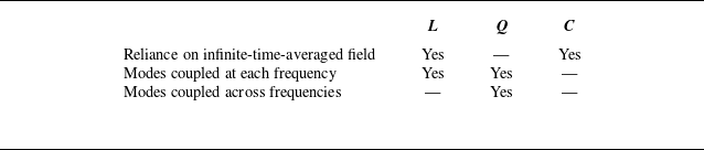
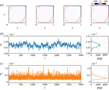
 Δt=0.4
 K
K K′
K′
 fk=0.586,1.211,1.797
 x
x
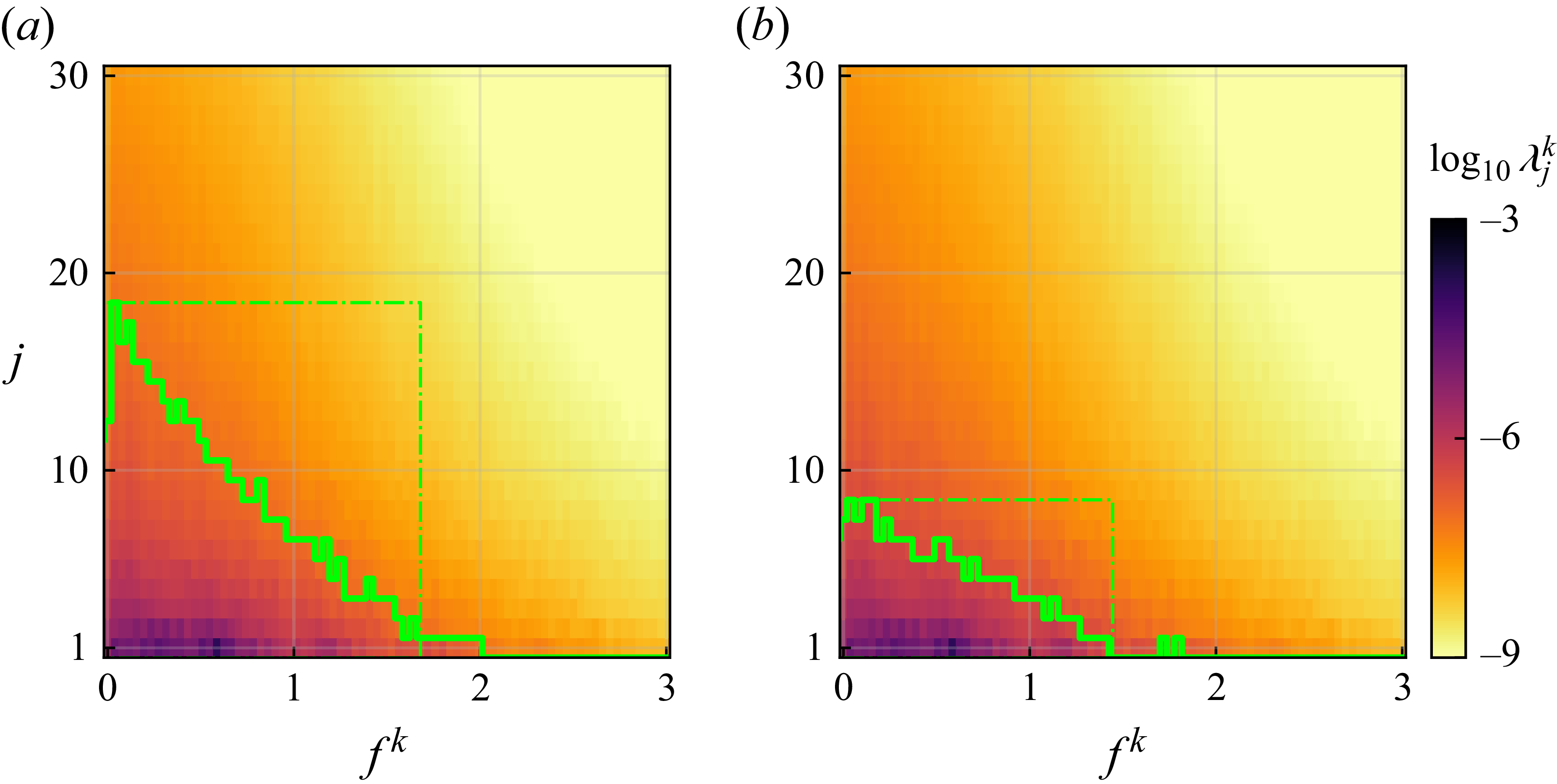


 J
J η
η ω
ω f15=0.587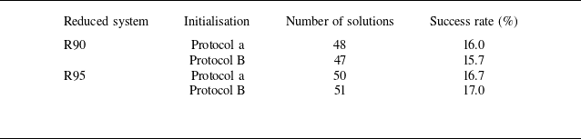
 ω
ω
 J
J ω
ω η
η
 a1k
a1k
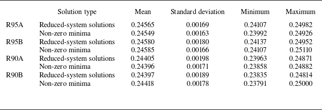
 J=0
J=0
 Ejk
Ejk
 a115
a115
 D
D K
K
 1000
1000 K
K D
D
 Δt/T=1/64
 K′
K′ K
K D
D


 Open access

