


1. Introduction
1.1. Motivation and literature review
Understanding the aerodynamics of porous bluff bodies is important for a wide range of engineering and biological applications including the design of parachutes (Peterson, Strickland & Higuchi Reference Peterson, Strickland and Higuchi1996) and meshes (Gomes-Fernandes, Ganapathisubramani & Vassilicos Reference Gomes-Fernandes, Ganapathisubramani and Vassilicos2012; Vita et al. Reference Vita, Hemida, Andrianne and Baniotopoulos2018), the flight of flower pappi (Cummins et al. Reference Cummins, Seale, Macente, Certini, Mastropaolo, Viola and Nakayama2018) and insects (Santhanakrishnan et al. Reference Santhanakrishnan, Robinson, Jones, Low, Gadi, Hedrick and Miller2014) and the design of buildings (Kim et al. Reference Kim, Sanders, Famiglietti and Guinot2015; Velickovic, Zech & Soares-Frazão Reference Velickovic, Zech and Soares-Frazão2017). Porous objects can also serve as models for more complicated systems. One such example is porous disks and the central role they play in wind energy modelling through actuator disk models, as they are simple alternatives to modelling detailed rotor aerodynamics (Sørensen Reference Sørensen2016; Ayati et al. Reference Ayati, Steiros, Miller, Duvvuri and Hultmark2019; Bempedelis & Steiros Reference Bempedelis and Steiros2022; Steiros, Bempedelis & Cicolin Reference Steiros, Bempedelis and Cicolin2022; Hunt et al. Reference Hunt, Athair, Williams and Polagye2024).
Introducing perforations on a bluff body can induce significant (and often unexpected) alterations of the flow physics, to the point that only very rudimentary effects of porosity are well modelled and understood. Outside of the wake, the flow can be approximated as irrotational and, therefore, modelled via potential flow theory (van Kuik Reference van Kuik2017; Steiros & Hultmark Reference Steiros and Hultmark2018; Shapiro, Gayme & Meneveau Reference Shapiro, Gayme and Meneveau2018). Turbulence in the inflow can be superimposed by assuming rapid distortion of the turbulent eddies (Graham Reference Graham2017). In contrast, the physics of the flow inside the wake is significantly more complex, and the complicated, nonlinear, interactions with turbulence cannot be omitted. In the wake, the inclusion of base bleeding (i.e. fluid entering the wake through the body) alters the mean flow topology and the associated flow instabilities. As bleeding is increased, the mean recirculation region of a porous body detaches from the body base and migrates downstream, until a critical value of porosity is reached where it completely disappears (Leal & Acrivos Reference Leal and Acrivos1969; Ledda et al. Reference Ledda, Siconolfi, Viola, Gallaire and Camarri2018; Steiros, Bempedelis & Ding Reference Steiros, Bempedelis and Ding2021). Wake bleeding has also a large impact on vortex shedding, weakening the vortices and rendering shedding more intermittent (Cicolin et al. Reference Cicolin, Chellini, Usherwood, Ganapathisubramani and Castro2024). At large degrees of bleeding, shedding completely disappears (Castro Reference Castro1971). Bleeding has also repercussions in the far wake, where the formation and evolution of the so-called secondary vortex street instability is altered (Cimbala, Nagib & Roshko Reference Cimbala, Nagib and Roshko1988; Bekoglu, Bempedelis & Steiros Reference Bekoglu, Bempedelis and Steiros2025).
The vast majority of previous studies on the flow associated with porous bodies have focused on porous flat plates (see, for instance, (De Bray Reference De Bray1957; Castro Reference Castro1971; Graham Reference Graham1976; Camp & Cal Reference Camp and Cal2016; Cicolin et al. Reference Cicolin, Chellini, Usherwood, Ganapathisubramani and Castro2024; Marchand et al. Reference Marchand, Ramananarivo, Duprat and Josserand2024; Steiros et al. Reference Steiros, Obligado, Bragança, Cuvier and Vassilicos2025; Bose, Bruce & Viola Reference Bose, Bruce and Viola2025)). The flow physics involved in flows around flat plates (porous or not) are arguably simpler than that around other bluff-body shapes. The separation points are uniquely set by the plate edges while the porosity distribution is single layered and flat. This (relative) lack of complexity has led to the development of several analytical models for flat plates (see, e.g. van Kuik Reference van Kuik2017; Steiros & Hultmark Reference Steiros and Hultmark2018; Marchand et al. Reference Marchand, Ramananarivo, Duprat and Josserand2024). Regarding other canonical bluff-body shapes, porous cylinders have also received some interest (Nicolle & Eames Reference Nicolle and Eames2011; Ledda et al. Reference Ledda, Siconolfi, Viola, Gallaire and Camarri2018; Steiros et al. Reference Steiros, Kokmanian, Bempedelis and Hultmark2020). For circular cylinders, the flow physics are more complex compared with the case of plates. The separation points are non-unique and depend on the local Reynolds number, while the distribution of porosity is three-dimensional and curved. Analytical modelling has been much more limited and confined to the case where the free-stream flow is only minimally perturbed by the bluff body, i.e. at very high body porosities (De Tavernier & Ferreira Reference De Tavernier and Ferreira2019).
Perhaps surprisingly, porous spheres have received significantly less attention, with previous research focusing almost exclusively on the very low-Reynolds-number regime, relevant to particle dynamics (Roy & Damiano Reference Roy and Damiano2008; Yu et al. Reference Yu, Zeng, Lee, Chen and Low2012). Reynolds number effects can be significant for porous bodies. For example, porous disks with a Reynolds number of $\textit {O}(100)$
have a maximum drag coefficient at non-zero porosity (Cummins et al. Reference Cummins, Viola, Mastropaolo and Nakayama2017), whereas the drag on homogeneously perforated disks at turbulent Reynolds numbers generally decreases with porosity (Robert Reference Robert1980). To the authors’ best knowledge, the flow physics of porous spheres exposed to turbulent Reynolds numbers has not hitherto been investigated. This is the focus of the present study. In particular, we study hollow porous spheres, which have recently received attention in the context of sport aerodynamics as an alternative to inflated sports balls (Newcomb Reference Newcomb2024). An important question is how perforation affects the aerodynamic resistance of the porous ball during flight. It is conventionally assumed that the homogeneous perforation of a hollow bluff body decreases its drag, with available experimental data of porous plates and cylinders generally supporting this postulation (Graham Reference Graham1976; Steiros & Hultmark Reference Steiros and Hultmark2018; Steiros et al. Reference Steiros, Kokmanian, Bempedelis and Hultmark2020).
$\textit {O}(100)$
have a maximum drag coefficient at non-zero porosity (Cummins et al. Reference Cummins, Viola, Mastropaolo and Nakayama2017), whereas the drag on homogeneously perforated disks at turbulent Reynolds numbers generally decreases with porosity (Robert Reference Robert1980). To the authors’ best knowledge, the flow physics of porous spheres exposed to turbulent Reynolds numbers has not hitherto been investigated. This is the focus of the present study. In particular, we study hollow porous spheres, which have recently received attention in the context of sport aerodynamics as an alternative to inflated sports balls (Newcomb Reference Newcomb2024). An important question is how perforation affects the aerodynamic resistance of the porous ball during flight. It is conventionally assumed that the homogeneous perforation of a hollow bluff body decreases its drag, with available experimental data of porous plates and cylinders generally supporting this postulation (Graham Reference Graham1976; Steiros & Hultmark Reference Steiros and Hultmark2018; Steiros et al. Reference Steiros, Kokmanian, Bempedelis and Hultmark2020).
1.2. Outline of the paper
This study presents an experimental investigation of the aerodynamics of hollow porous spheres at moderate to high Reynolds numbers. In § 2 a preliminary free-fall experiment is presented to test whether homogeneous perforation decreases or increases drag. The free-fall experiment is followed by a systematic wind tunnel investigation. The wind tunnel experimental procedure is outlined in § 3. Wind tunnel drag coefficient measurements are analysed for Reynolds number and porosity effects in § 4. The effect of porosity on the mean flow and turbulence kinetic energy distribution is analysed from flow field measurements in § 5. Changes in the separation point and subsequent effects on drag are analysed in § 6. In § 7 we consider an energy budget for the entire flow, matching the input power required to drive a porous bluff body through quiescent fluid to kinetic energy dissipation. We apply this analysis to compare porous spheres to other porous bluff bodies. In § 8 the conclusions of the study are drawn.
2. Drag on a sphere increases with porosity
A preliminary experiment was devised to test whether homogeneous perforation decreases drag on a sphere: two spheres of different porosities were dropped simultaneously from a height of 45 $\pm$
5 m. Spheres of diameter 230 mm and porosities 2 % and 46 % were 3D printed out of thermoplastic polyurethane, where the porosity is the fraction of surface area removed. The mass of each sphere was matched to within 5 %. A top view of the experimental setup is shown in figure 1(a) with the porosity for each sphere indicated. The string connecting the spheres was cut and the free-fall trajectory was recorded. The camera field-of-view is shown in figure 1(b). As seen in the zoomed-in view the more porous sphere hits the ground significantly later, indicating higher drag. The time difference between ground impact of the two spheres can be accurately measured from the video by manual inspection. From two trials, the measured time difference between impacts was 0.42
$\pm$
5 m. Spheres of diameter 230 mm and porosities 2 % and 46 % were 3D printed out of thermoplastic polyurethane, where the porosity is the fraction of surface area removed. The mass of each sphere was matched to within 5 %. A top view of the experimental setup is shown in figure 1(a) with the porosity for each sphere indicated. The string connecting the spheres was cut and the free-fall trajectory was recorded. The camera field-of-view is shown in figure 1(b). As seen in the zoomed-in view the more porous sphere hits the ground significantly later, indicating higher drag. The time difference between ground impact of the two spheres can be accurately measured from the video by manual inspection. From two trials, the measured time difference between impacts was 0.42 $\,\pm\, 0.017$
seconds and 0.38
$\,\pm\, 0.017$
seconds and 0.38 $\,\pm\, 0.017$
seconds compared with the total free-fall time of approximately 3.25 s. The drop test experiments unequivocally support increased aerodynamic drag with porosity.
$\,\pm\, 0.017$
seconds compared with the total free-fall time of approximately 3.25 s. The drop test experiments unequivocally support increased aerodynamic drag with porosity.

Figure 1. Drop test experiments showing that drag can increase with porosity for a sphere. (a) Top view of drop apparatus with sphere porosity indicated. (b) Full view of free fall, including zoomed-in view shortly before impact with the ground. The more porous sphere is approximately 6 m behind, indicating higher drag.
3. Wind tunnel experimental campaign
To systematically investigate the effect of porosity on the aerodynamics of a sphere, wind tunnel measurements were conducted in a 1.2 m $\times$
1.2 m cross-section closed circuit wind tunnel at Princeton University. The turbulence intensity in the test section is 0.03 % and the mean flow uniformity is
$\times$
1.2 m cross-section closed circuit wind tunnel at Princeton University. The turbulence intensity in the test section is 0.03 % and the mean flow uniformity is $\pm 1\,\%$
. A detailed description of the wind tunnel can be found in Breuer et al. (Reference Breuer, Drela, Fan and Di Luca2022). Drag coefficients were recorded as a function of Reynolds number and porosity using two different mounting configurations. In the first configuration the spheres were mounted via a rear string, and in the second configuration, the spheres were mounted to the side of the wind tunnel. Each configuration used distinct mounting and force sampling hardware. A rear string is considered best practice for sphere drag measurements to avoid string interference with boundary layer separation (Hoerner Reference Hoerner1935). The side-mounted configuration is preferable for wake flow field measurements so that the string is not in the camera field of view. Flow field measurements at varying porosity and a fixed Reynolds number were conducted in the side-mounted configuration. Drag measurements with a separation ring were made in the side-mounted configuration to test hypotheses generated from the flow field analysis.
$\pm 1\,\%$
. A detailed description of the wind tunnel can be found in Breuer et al. (Reference Breuer, Drela, Fan and Di Luca2022). Drag coefficients were recorded as a function of Reynolds number and porosity using two different mounting configurations. In the first configuration the spheres were mounted via a rear string, and in the second configuration, the spheres were mounted to the side of the wind tunnel. Each configuration used distinct mounting and force sampling hardware. A rear string is considered best practice for sphere drag measurements to avoid string interference with boundary layer separation (Hoerner Reference Hoerner1935). The side-mounted configuration is preferable for wake flow field measurements so that the string is not in the camera field of view. Flow field measurements at varying porosity and a fixed Reynolds number were conducted in the side-mounted configuration. Drag measurements with a separation ring were made in the side-mounted configuration to test hypotheses generated from the flow field analysis.
3.1. Models and manufacturing
To accommodate convenient porosity changes, a solid frame with interchangeable panels, which when assembled yields a sphere, was used (shown in figure 2
a). The sphere has diameter $D$
= 150 mm with 12 pentagonal and 20 hexagonal openings. Curved panels insert into the openings of the frame and porosity was varied by using holes of varying diameters in the panels. Here, porosity is defined as
$D$
= 150 mm with 12 pentagonal and 20 hexagonal openings. Curved panels insert into the openings of the frame and porosity was varied by using holes of varying diameters in the panels. Here, porosity is defined as
 \begin{align} \beta = \frac {A_o}{\pi D^2}, \end{align}
where $A_o$
is the total open area introduced by the holes. The pentagonal panels had six holes and the hexagonal panels had seven holes. The radii of the holes in each panel type were scaled such that the porosity of the pentagonal and hexagonal panels was equal. As a result, the porosity distribution was approximately homogeneous. Hole radii and tested porosities can be found in table 1. For the highest porosity case, all panels were removed, leaving only the frame. One pentagonal panel was maintained solid for mounting the sphere to a string via a threaded insert. The solid mounting panel was neglected in the porosity calculation because the impact on drag is deemed negligible from force measurements in different orientations.
$A_o$
is the total open area introduced by the holes. The pentagonal panels had six holes and the hexagonal panels had seven holes. The radii of the holes in each panel type were scaled such that the porosity of the pentagonal and hexagonal panels was equal. As a result, the porosity distribution was approximately homogeneous. Hole radii and tested porosities can be found in table 1. For the highest porosity case, all panels were removed, leaving only the frame. One pentagonal panel was maintained solid for mounting the sphere to a string via a threaded insert. The solid mounting panel was neglected in the porosity calculation because the impact on drag is deemed negligible from force measurements in different orientations.
Table 1. Geometric characteristics of manufactured spheres.


Figure 2. Wind tunnel experimental campaign. (a) Frame and panel design. (b) Rear-mounted configuration inside the tunnel. The minimum and maximum string diameter is indicated. Here ‘M. P.’ denotes mounting panel. (c) Side-mounted configuration outside the tunnel. (d) Side-mounted sphere installed in the tunnel with separation ring. View from inside the tunnel. (e) Rendering of side-mounted configuration with PIV laser sheet. The camera (not shown) is opposite to the sphere.
The frame was 3D printed using Nylon 12 Powder. The panels were printed using a polylactic acid filament. When inserted into the frame, the panels are not perfectly flush, introducing a roughness scale of 250 $\unicode{x03BC}$
m (
$\unicode{x03BC}$
m ( $ 1.7 \times 10^{-3} D$
). The frame can also be fitted with a ring that, when positioned, induces flow separation at a fixed location. The interior diameter of the separation ring is 150 mm and the outer diameter is 157.6 mm so that the ring protrudes 0.05
$ 1.7 \times 10^{-3} D$
). The frame can also be fitted with a ring that, when positioned, induces flow separation at a fixed location. The interior diameter of the separation ring is 150 mm and the outer diameter is 157.6 mm so that the ring protrudes 0.05 $D$
from the sphere surface.
$D$
from the sphere surface.
3.2. Force measurements
In the rear-mounted configuration, models were mounted as shown in figure 2(b) to an AEROLAB strain gauge force balance. The boundary layer height on the side wall of the tunnel at the sphere location is, at most, 5 cm, so that the spheres in the centre of the tunnel are at least 13 boundary layer heights from the wall. For each porosity, the force balance was tared in a no-flow condition before varying the free-stream speed $U_{\infty }$
from 5 to 40 m s−1. Force data was sampled at 250 Hz for 10 s at each porosity and free-stream velocity. The sampling period was at least 330 advective time scales (
$U_{\infty }$
from 5 to 40 m s−1. Force data was sampled at 250 Hz for 10 s at each porosity and free-stream velocity. The sampling period was at least 330 advective time scales ( $D/U_{\infty }$
). The drag force
$D/U_{\infty }$
). The drag force $F_d$
was computed by averaging over the sampling period. Each measurement was repeated three times. Between repetitions, the model was removed and remounted to the string. The drag force on the string (without a sphere) was measured and was always less than 2 % of the sphere drag for the same free-stream velocity. With a sphere in place, the string drag is even smaller because it is in the wake of the sphere; thus, the string drag can be neglected in the rear-mounted configuration. In this configuration the mounting panel was oriented normal to the free stream. It is hypothesised that the solid mounting panel may positively bias drag measurements at high porosity because the flow encounters a solid plate normal to the flow after entering the fore of the sphere.
$F_d$
was computed by averaging over the sampling period. Each measurement was repeated three times. Between repetitions, the model was removed and remounted to the string. The drag force on the string (without a sphere) was measured and was always less than 2 % of the sphere drag for the same free-stream velocity. With a sphere in place, the string drag is even smaller because it is in the wake of the sphere; thus, the string drag can be neglected in the rear-mounted configuration. In this configuration the mounting panel was oriented normal to the free stream. It is hypothesised that the solid mounting panel may positively bias drag measurements at high porosity because the flow encounters a solid plate normal to the flow after entering the fore of the sphere.
A second mounting configuration was used to determine the effect of the mounting panel orientation and to enable flow field measurements in the sphere wake. Models were mounted on a string extending from the side wall of the tunnel. In this configuration the mounting panel was parallel instead of normal to the free stream. The boundary layer height at the model location in the side-mounted configuration is, at most, 9 cm, which can be compared with the string length of 17 cm. To verify that the tunnel boundary layer does not impact the trends in drag, drag coefficient measurements from the rear-mounted and side-mounted configurations are compared in § 4. The string was connected to a six degree-of-freedom ATI gamma force/torque transducer with 6.25 $\times$
10
$\times$
10 $^{-3}$
N resolution. A photograph of the mounting set-up outside the tunnel is shown in figure 2(c). For each porosity, the sphere was mounted inside the tunnel and the free-stream speed
$^{-3}$
N resolution. A photograph of the mounting set-up outside the tunnel is shown in figure 2(c). For each porosity, the sphere was mounted inside the tunnel and the free-stream speed $U_{\infty }$
was varied from 5 to 30 m s−1. The force transducer was tared in a no-flow condition between each free-stream velocity. Three-axis force data were sampled at 1000 Hz for a sample period of 10 s at each free-stream velocity and porosity. The drag force on the string was not negligible in the side-mounted configuration, so the drag on the string was measured without a sphere and subtracted from the measurements. Experiments with a separation ring were conducted in the side-mounted configuration using the same procedure. A sphere with the separation ring installed is shown in figure 2(d).
$U_{\infty }$
was varied from 5 to 30 m s−1. The force transducer was tared in a no-flow condition between each free-stream velocity. Three-axis force data were sampled at 1000 Hz for a sample period of 10 s at each free-stream velocity and porosity. The drag force on the string was not negligible in the side-mounted configuration, so the drag on the string was measured without a sphere and subtracted from the measurements. Experiments with a separation ring were conducted in the side-mounted configuration using the same procedure. A sphere with the separation ring installed is shown in figure 2(d).
The drag force was normalised by the free-stream dynamic pressure $\rho U_{\infty }^2/2$
and sphere frontal area
$\rho U_{\infty }^2/2$
and sphere frontal area $A = \pi D^2/4$
, yielding the drag coefficient
$A = \pi D^2/4$
, yielding the drag coefficient
 \begin{align} C_d = \frac {F_d}{ \dfrac {1}{2} \rho U_{\infty }^2 A}. \end{align}
The drag coefficient is measured as a function of the Reynolds number
 \begin{align} \textit{Re} = \frac {\rho U_{\infty } D}{\mu } \end{align}
and porosity $\beta$
. Here
$\beta$
. Here $\rho$
is the density and
$\rho$
is the density and $\mu$
is the dynamic viscosity.
$\mu$
is the dynamic viscosity.
3.3. Flow field measurements
Particle image velocimetry (PIV) measurements were conducted at a fixed Reynolds number $\textit{Re} = 1.54 \times 10^5$
and porosities
$\textit{Re} = 1.54 \times 10^5$
and porosities $\beta \in \{2\,\%, 9\,\%, 19\,\%, 36\,\%, 46\,\%, 80\,\%\}$
to visualise the flow fields in the side-mounted configuration. The PIV plane was the mid-span plane of the sphere. A rendering of the set-up and laser sheet is shown in figure 2(e). The particles were illuminated using a Photonics DMX high-speed Nd:YLF 527 nm dual cavity high-repetition laser with an acquisition rate of 650 Hz. The laser was located atop the wind tunnel and directed into the test section using a series of 90
$\beta \in \{2\,\%, 9\,\%, 19\,\%, 36\,\%, 46\,\%, 80\,\%\}$
to visualise the flow fields in the side-mounted configuration. The PIV plane was the mid-span plane of the sphere. A rendering of the set-up and laser sheet is shown in figure 2(e). The particles were illuminated using a Photonics DMX high-speed Nd:YLF 527 nm dual cavity high-repetition laser with an acquisition rate of 650 Hz. The laser was located atop the wind tunnel and directed into the test section using a series of 90 $^\circ$
mirrors. The beam was expanded into a sheet of thickness less than 2 mm with a 10 mm cylindrical lens. The flow was seeded with di-ethyl-hexyl-sebacat particles having a mean diameter 1
$^\circ$
mirrors. The beam was expanded into a sheet of thickness less than 2 mm with a 10 mm cylindrical lens. The flow was seeded with di-ethyl-hexyl-sebacat particles having a mean diameter 1 $\unicode{x03BC}$
m. Image pairs were acquired using a Photron Nova R5 high-speed CMOS camera operating in double frame mode. A total number of 1000 frame pairs were recorded for each test case. Multipass cross-correlation was used to extract velocity fields from the frame pairs (implemented in LaVision’s DaVis software). Two PIV campaigns were conducted. In the first campaign (
$\unicode{x03BC}$
m. Image pairs were acquired using a Photron Nova R5 high-speed CMOS camera operating in double frame mode. A total number of 1000 frame pairs were recorded for each test case. Multipass cross-correlation was used to extract velocity fields from the frame pairs (implemented in LaVision’s DaVis software). Two PIV campaigns were conducted. In the first campaign ( $\beta \in \{2\,\%, 36\,\%,80\,\%\}$
), the image resolution was 9.4 MP and the field of view was centred on the sphere, with limits
$\beta \in \{2\,\%, 36\,\%,80\,\%\}$
), the image resolution was 9.4 MP and the field of view was centred on the sphere, with limits $\pm 1.1D$
in the streamwise direction and
$\pm 1.1D$
in the streamwise direction and $\pm 0.63D$
in the vertical direction. Shadows cast by the sphere limit PIV measurements to the top half of the sphere with the specified laser illumination. In the second PIV campaign (
$\pm 0.63D$
in the vertical direction. Shadows cast by the sphere limit PIV measurements to the top half of the sphere with the specified laser illumination. In the second PIV campaign ( $\beta \in \{9\,\%, 19\,\%, 46\,\%\}$
), the image resolution was 6.5 MP and the field of view was shifted to focus on the top half of the sphere, extending from −
$\beta \in \{9\,\%, 19\,\%, 46\,\%\}$
), the image resolution was 6.5 MP and the field of view was shifted to focus on the top half of the sphere, extending from − $0.49D$
to 0.73
$0.49D$
to 0.73 $D$
in the vertical direction. The final side lengths of the PIV interrogation windows were 24 and 16 pixels for each campaign, respectively. With 50 % overlap, the velocity vector spacings are 0.54 % and 0.64 % of the sphere diameter, respectively.
$D$
in the vertical direction. The final side lengths of the PIV interrogation windows were 24 and 16 pixels for each campaign, respectively. With 50 % overlap, the velocity vector spacings are 0.54 % and 0.64 % of the sphere diameter, respectively.

Figure 3. (a) Drag coefficient as a function of Reynolds number for the rear-mounted configuration. Shading indicates sample standard deviation from repeated trials. Every other point is marked for clarity. (b) Drag coefficient as a function of porosity. Rear-mounted configuration in circles and side-mounted configuration in squares. Shading indicates that the Reynolds number applies to both markers. The dashed line connects points where PIV was conducted.
4. Reynolds number and porosity effects on drag
Drag coefficient measurements are shown in figure 3(a) as a function of Reynolds number for the rear-mounted configuration. For the two lowest porosity cases, the trend is consistent with a drag crisis for rough spheres (Achenbach Reference Achenbach1974). Comparison of $\beta = 0\,\%$
and
$\beta = 0\,\%$
and $\beta = 2\,\%$
suggests that adding a small amount of porosity is qualitatively similar to a roughness effect. The critical Reynolds number decreases and the supercritical drag coefficient increases. A lowered critical Reynolds number suggests the boundary layer is perturbed by the presence of porosity, but the precise nature of this perturbation cannot be determined from the present data. In contrast to the abrupt decrease in drag at lower porosity, relatively weak Reynolds number effects are observed for 9 % porosity. In general, the higher porosity cases (
$\beta = 2\,\%$
suggests that adding a small amount of porosity is qualitatively similar to a roughness effect. The critical Reynolds number decreases and the supercritical drag coefficient increases. A lowered critical Reynolds number suggests the boundary layer is perturbed by the presence of porosity, but the precise nature of this perturbation cannot be determined from the present data. In contrast to the abrupt decrease in drag at lower porosity, relatively weak Reynolds number effects are observed for 9 % porosity. In general, the higher porosity cases ( $\beta \geq 9\,\%$
) are insensitive to the Reynolds number when
$\beta \geq 9\,\%$
) are insensitive to the Reynolds number when $\textit{Re} \geq 1.5 \times 10^5$
. On the other hand, within this parameter regime, porosity significantly influences drag.
$\textit{Re} \geq 1.5 \times 10^5$
. On the other hand, within this parameter regime, porosity significantly influences drag.

Figure 4. Mean streamwise velocity $U$
at the mid-span plane for
$U$
at the mid-span plane for $ \textit{Re} = 1.54 \times 10^5$
at varying porosity. The streamwise direction is
$ \textit{Re} = 1.54 \times 10^5$
at varying porosity. The streamwise direction is $x$
and the vertical is
$x$
and the vertical is $y$
with the origin at the sphere centre.
$y$
with the origin at the sphere centre.
In figure 3(b) the drag coefficient for the rear-mounted configuration is plotted in circles against porosity for supercritical Reynolds numbers ( $\textit{Re} \geq 1.5 \times 10^5$
). A trend of increasing drag with porosity up to 80 % is observed. Further increases in porosity could not be accomplished with the current design but there must be a steep decline in drag at high porosity to enforce
$\textit{Re} \geq 1.5 \times 10^5$
). A trend of increasing drag with porosity up to 80 % is observed. Further increases in porosity could not be accomplished with the current design but there must be a steep decline in drag at high porosity to enforce $C_d \to 0$
as
$C_d \to 0$
as $\beta \to 1$
. As further discussed in Appendix A, the primary effect of the side-mounted string is to weaken the critical regime (i.e. the effect is limited to
$\beta \to 1$
. As further discussed in Appendix A, the primary effect of the side-mounted string is to weaken the critical regime (i.e. the effect is limited to $\beta \leq 2\,\%$
). Drag coefficients from the side-mounted configuration are plotted in figure 3(b) for sufficiently high Reynolds numbers where critical regime effects play a minor role (
$\beta \leq 2\,\%$
). Drag coefficients from the side-mounted configuration are plotted in figure 3(b) for sufficiently high Reynolds numbers where critical regime effects play a minor role ( $\textit{Re} \geq 2 \times 10^5$
for
$\textit{Re} \geq 2 \times 10^5$
for $\beta = 0\,\%$
and
$\beta = 0\,\%$
and $ \textit{Re} \geq 1.5 \times 10^5$
for
$ \textit{Re} \geq 1.5 \times 10^5$
for $\beta = 2\,\%$
). The dashed line in figure 3(b) connects points where PIV was conducted in the side-mounted configuration. Good agreement with the trend of the rear-mounted configuration is observed. Therefore, the side-mounted drag data corroborate the trend of increasing drag with porosity up to
$\beta = 2\,\%$
). The dashed line in figure 3(b) connects points where PIV was conducted in the side-mounted configuration. Good agreement with the trend of the rear-mounted configuration is observed. Therefore, the side-mounted drag data corroborate the trend of increasing drag with porosity up to $\beta = 80\,\%$
. This trend, which is consistent with the drop test experiments and contrary to other bluff bodies, is the focus of the present study.
$\beta = 80\,\%$
. This trend, which is consistent with the drop test experiments and contrary to other bluff bodies, is the focus of the present study.
5. Effect of porosity on the flow field
5.1. Mean flow
Contours of the streamwise mean velocity $U$
are shown in figure 4 to illustrate the basic effect of porosity on the mean flow. As porosity increases, more fluid passes through the fore of the sphere and bleeds through the surface into the wake. At
$U$
are shown in figure 4 to illustrate the basic effect of porosity on the mean flow. As porosity increases, more fluid passes through the fore of the sphere and bleeds through the surface into the wake. At $\beta = 2\,\%$
(figure 4
a), the wake contains a diameter-scale contiguous reversed flow region attached to the aft of the sphere. With increasing porosity, jets form in the wake, breaking up the reversed flow region. For
$\beta = 2\,\%$
(figure 4
a), the wake contains a diameter-scale contiguous reversed flow region attached to the aft of the sphere. With increasing porosity, jets form in the wake, breaking up the reversed flow region. For $9\,\% \leq \beta \leq 46\,\%$
(figure 4
b–e), the wake bleeding strengthens with porosity, but there is still a reversed flow region immediately aft of the sphere. In the highest porosity case, smaller wakes can be observed behind individual frame elements (figure 4
f). The increase in wake bleeding with porosity for a sphere is qualitatively similar to previous flat plate observations (Castro Reference Castro1971; Cicolin et al. Reference Cicolin, Chellini, Usherwood, Ganapathisubramani and Castro2024).
$9\,\% \leq \beta \leq 46\,\%$
(figure 4
b–e), the wake bleeding strengthens with porosity, but there is still a reversed flow region immediately aft of the sphere. In the highest porosity case, smaller wakes can be observed behind individual frame elements (figure 4
f). The increase in wake bleeding with porosity for a sphere is qualitatively similar to previous flat plate observations (Castro Reference Castro1971; Cicolin et al. Reference Cicolin, Chellini, Usherwood, Ganapathisubramani and Castro2024).

Figure 5. Normalised turbulent kinetic energy at the mid-span plane for $ \textit{Re} = 1.54 \times 10^5$
at varying porosity. The streamwise direction is
$ \textit{Re} = 1.54 \times 10^5$
at varying porosity. The streamwise direction is $x$
and the vertical is
$x$
and the vertical is $y$
with the origin at the sphere centre.
$y$
with the origin at the sphere centre.
5.2. Turbulent kinetic energy
Contours of the turbulent kinetic energy $k$
are shown in figure 5 as a function of porosity. Here
$k$
are shown in figure 5 as a function of porosity. Here $k = ( 2\langle u_y^2 \rangle + \langle u_x^2\rangle )$
with
$k = ( 2\langle u_y^2 \rangle + \langle u_x^2\rangle )$
with $\langle u_y^2\rangle$
and
$\langle u_y^2\rangle$
and $\langle u_x^2 \rangle$
the velocity variance in the vertical and streamwise directions, respectively. The factor of two on
$\langle u_x^2 \rangle$
the velocity variance in the vertical and streamwise directions, respectively. The factor of two on $\langle u_y^2 \rangle$
reflects the assumption that the out-of-plane variance is approximately equal to the vertical variance. Two prominent structures are seen to dominate the
$\langle u_y^2 \rangle$
reflects the assumption that the out-of-plane variance is approximately equal to the vertical variance. Two prominent structures are seen to dominate the $k$
fields: (i) turbulence generated by flow exiting the pores, and (ii) a turbulent shear layer forming at the outer edge of a body. For
$k$
fields: (i) turbulence generated by flow exiting the pores, and (ii) a turbulent shear layer forming at the outer edge of a body. For $\beta \geq 9\,\%$
(figure 5
b–f), there is a clear monotonic growth in turbulence from flow exiting the pores as porosity increases. This suggests there may be a connection between increased turbulence from flow exiting the pores and increased drag for
$\beta \geq 9\,\%$
(figure 5
b–f), there is a clear monotonic growth in turbulence from flow exiting the pores as porosity increases. This suggests there may be a connection between increased turbulence from flow exiting the pores and increased drag for $\beta \geq 9\,\%$
. Enhanced wake turbulence has previously been linked to increased drag (Mathai et al. Reference Mathai, Das, Naylor and Breuer2023). With the exception of
$\beta \geq 9\,\%$
. Enhanced wake turbulence has previously been linked to increased drag (Mathai et al. Reference Mathai, Das, Naylor and Breuer2023). With the exception of $\beta = 80\,\%$
(where no shear layer can be distinguished), trends in the turbulent shear are more difficult to discern from figure 5 because of the limited field of view. Development of the turbulent shear layer may be pushed downstream with increasing porosity. In § 7 the contributions of the body-scale shear layer and losses from flow exiting the pores to drag are further examined for
$\beta = 80\,\%$
(where no shear layer can be distinguished), trends in the turbulent shear are more difficult to discern from figure 5 because of the limited field of view. Development of the turbulent shear layer may be pushed downstream with increasing porosity. In § 7 the contributions of the body-scale shear layer and losses from flow exiting the pores to drag are further examined for $\beta \geq 9\,\%$
.
$\beta \geq 9\,\%$
.
First we consider the mechanism for higher drag at 9 % porosity compared with 2 % porosity. For these two cases, no distinct turbulence generated from flow exiting the pores can be observed. Contrary to the increase in drag with porosity, lower wake turbulence is observed at 9 % porosity compared with 2 % porosity (figures 5 a and 5 b). However, examining the origin of the turbulent shear layer in figures 5(a) and 5(b) suggests that the separation point may also change with porosity.
6. Effect of porosity on flow separation
In a flat plate the separation points are fixed by sharp edges. This is not the case for a sphere. In this section we examine whether shifts in the separation point can explain the observed changes in drag with porosity. We first consider whether separation is occurring, as typically understood for a solid body, at high porosity. Next we analyse the surface-normal velocity distribution at different porosities to infer shifts in the separation point. Finally, drag measurements with a separation ring are used to test predictions based on analysis of the flow fields.
6.1. Effect of porosity on material spike formation
The concept of separation, as typically understood for a solid body, is questionable at high porosity. With increasing porosity the flow may pass through the forward surface of the sphere instead of being diverted around the body. To be clear, separation can still occur off of individual solid elements at high porosity. In the latter case, a macroscopic separation point (e.g. measured by the separation angle) is ill-defined. To distinguish between these phenomena requires defining separation. Recognising that separation is, in general, an expulsion of fluid material away from a surface, several works have considered theories of separation defined by the properties of points or a line that move with the flow, i.e. material particles and lines (Haller Reference Haller2004; Surana et al. Reference Surana, Grunberg and Haller2006, Reference Surana, Jacobs, Grunberg and Haller2008; Serra et al. Reference Serra, Vétel and Haller2018, Reference Serra, Crouzat, Simon, Vétel and Haller2020). A central concept is that separation involves the formation of a `material spike’. Serra, Vétel & Haller (Reference Serra, Vétel and Haller2018) defined a material spike by the formation of a characteristic cusp when material lines that are initially parallel to a surface are advected by the flow. This theory has been shown to be quite general, capturing separation in flows with arbitrary time dependence (Serra et al. Reference Serra, Vétel and Haller2018). We analyse material spike formation at different porosities to determine if there is a qualitative shift in separation behaviour.
Figure 6 shows material lines that are initially at constant radial distances from $0.53D$
to
$0.53D$
to $0.575D$
after advecting forward in time by the mean velocity field for a time
$0.575D$
after advecting forward in time by the mean velocity field for a time $2D/U_{\infty }$
. A supplementary movie showing the full evolution of material lines is available at https://doi.org/10.1017/jfm.2025.11080. We take the case of
$2D/U_{\infty }$
. A supplementary movie showing the full evolution of material lines is available at https://doi.org/10.1017/jfm.2025.11080. We take the case of $\beta = 2\,\%$
as a baseline. The abrupt decrease in drag with increasing Reynolds number observed in figure 3(a) indicates that separation occurs similarly to a solid sphere at this porosity. In figure 6(a) there is a corresponding spike formed by the advected material lines. At 9 % porosity a similar spike is observed (figure 6
b). With further increases in porosity (figure 6
c–f) the material spike is qualitatively similar until 80 % porosity (figure 6
f), where it is less pronounced than the lower porosity cases. Analysis of material spike formation suggests that the macroscopic separation physics do not change qualitatively up to 46 % porosity, while at 80 % porosity a material spike is less distinct.
$\beta = 2\,\%$
as a baseline. The abrupt decrease in drag with increasing Reynolds number observed in figure 3(a) indicates that separation occurs similarly to a solid sphere at this porosity. In figure 6(a) there is a corresponding spike formed by the advected material lines. At 9 % porosity a similar spike is observed (figure 6
b). With further increases in porosity (figure 6
c–f) the material spike is qualitatively similar until 80 % porosity (figure 6
f), where it is less pronounced than the lower porosity cases. Analysis of material spike formation suggests that the macroscopic separation physics do not change qualitatively up to 46 % porosity, while at 80 % porosity a material spike is less distinct.
6.2. Effect of porosity on the separation point
Contours of the mean surface-normal (radial) velocity $U_r$
are shown in figure 6. Dashed lines indicate the angle
$U_r$
are shown in figure 6. Dashed lines indicate the angle $\theta$
from the front of the sphere. Note that reflections limit measurements to radial distances
$\theta$
from the front of the sphere. Note that reflections limit measurements to radial distances $0.03D$
from the sphere surface (see Appendix B) so that the boundary layer cannot be directly observed. For each porosity, the surface-normal velocity shifts from predominantly negative to positive with increasing
$0.03D$
from the sphere surface (see Appendix B) so that the boundary layer cannot be directly observed. For each porosity, the surface-normal velocity shifts from predominantly negative to positive with increasing $\theta$
. Comparing
$\theta$
. Comparing $\beta =2\,\%$
and
$\beta =2\,\%$
and $\beta = 9\,\%$
(figures 6
a and 6
b) we observe that the zero radial velocity region is brought forward by 10
$\beta = 9\,\%$
(figures 6
a and 6
b) we observe that the zero radial velocity region is brought forward by 10 $^{\circ }$
, suggesting earlier separation with increasing porosity. Consequently, the increase in drag coefficient from
$^{\circ }$
, suggesting earlier separation with increasing porosity. Consequently, the increase in drag coefficient from $\beta = 2\,\%$
to
$\beta = 2\,\%$
to $\beta = 9\,\%$
at supercritical Reynolds numbers is plausibly explained by earlier separation. However, further increases in porosity have weak effects on the inferred separation point up to
$\beta = 9\,\%$
at supercritical Reynolds numbers is plausibly explained by earlier separation. However, further increases in porosity have weak effects on the inferred separation point up to $\beta = 46\,\%$
(figure 6
b–e).
$\beta = 46\,\%$
(figure 6
b–e).

Figure 6. Porosity effects on separation for $ \textit{Re} = 1.54 \times 10^5$
. Thick solid lines are material lines initially at constant radial distances from
$ \textit{Re} = 1.54 \times 10^5$
. Thick solid lines are material lines initially at constant radial distances from $r/D = 0.53$
to
$r/D = 0.53$
to $0.575$
after advecting forward in time by the mean velocity field for a time
$0.575$
after advecting forward in time by the mean velocity field for a time $2D/U_{\infty }$
. Dashed lines indicate the angle from the front of the sphere. Contours of surface-normal velocity
$2D/U_{\infty }$
. Dashed lines indicate the angle from the front of the sphere. Contours of surface-normal velocity $U_r$
are shown by colour and thin lines.
$U_r$
are shown by colour and thin lines.
In the highest porosity case, the zero radial velocity region shifts aft again (figure 6
f). This shift is in contrast to the observed increase in drag from figure 3(a), suggesting that (consistent with the previous section) the location of the separation point is less relevant to drag at 80 % porosity. A potential explanation is that the highest porosity case is better characterised as a double grid than a sphere. With increasing porosity, we expect that a length scale based on the pore diameter, or spacing between pores, will become increasingly relevant to the flow physics. At the same time, the importance of the body scale (e.g. sphere diameter) will diminish. At sufficiently high porosity we expect that the flow is comprised of interacting structures commensurate with the pore scale. This characterisation is consistent with figure 4(f), where wakes from individual bars that make up the frame are observed for $\beta = 80\,\%$
. A wake on the scale of the sphere diameter, where the surface pressure takes a constant value set by the separation point (Achenbach Reference Achenbach1972), is largely absent. Thus, we hypothesise that, at
$\beta = 80\,\%$
. A wake on the scale of the sphere diameter, where the surface pressure takes a constant value set by the separation point (Achenbach Reference Achenbach1972), is largely absent. Thus, we hypothesise that, at $\beta = 80\,\%$
, the separation point location does not dictate the base pressure or, as a consequence, the drag. This shift in the flow physics regime, towards dominance of the pore scale, is further discussed in § 7.
$\beta = 80\,\%$
, the separation point location does not dictate the base pressure or, as a consequence, the drag. This shift in the flow physics regime, towards dominance of the pore scale, is further discussed in § 7.
6.3. Porosity effects on drag with a fixed separation point
For sufficiently low porosities where the separation point does play a role in dictating drag ( $\beta \lt 80\,\%$
), we further test the conclusions of the previous section using a separation ring. Analysis of surface-normal flow in the previous section suggests the following: (i) the increase in drag from
$\beta \lt 80\,\%$
), we further test the conclusions of the previous section using a separation ring. Analysis of surface-normal flow in the previous section suggests the following: (i) the increase in drag from $\beta = 2\,\%$
to
$\beta = 2\,\%$
to $\beta = 9\,\%$
is primarily caused by a shift in the separation point, and (ii) separation point shifts do not explain drag increases for
$\beta = 9\,\%$
is primarily caused by a shift in the separation point, and (ii) separation point shifts do not explain drag increases for $9\,\% \leq \beta \leq 46\,\%$
. However, the time-averaged flow fields of the previous section cannot capture the exact location of the separation point nor its quantitative effect on the drag. To test the validity of the above points, drag measurements with a separation ring, fixing the separation point at
$9\,\% \leq \beta \leq 46\,\%$
. However, the time-averaged flow fields of the previous section cannot capture the exact location of the separation point nor its quantitative effect on the drag. To test the validity of the above points, drag measurements with a separation ring, fixing the separation point at $\theta = 90^{\circ }$
, were conducted. In figure 7(a) the drag coefficient with the separation ring
$\theta = 90^{\circ }$
, were conducted. In figure 7(a) the drag coefficient with the separation ring $C_d^R$
is shown as a function of porosity.
$C_d^R$
is shown as a function of porosity.
If the increase in drag from 2 % to 9 % porosity is primarily caused by a shift in the separation point then we expect that fixing the separation point will reduce the increase in drag. Indeed, figure 7(a) shows that the drag coefficient of the ring-fitted sphere varies only slightly between 2 % and 9 % porosity (compared with the case without the ring in figure 3
b). Figure 7(a) also strongly supports the hypothesis that separation point shifts are insufficient to explain drag increases for $9\,\% \leq \beta \leq 46\,\%$
. When the ring is equipped, the separation point is fixed and drag still increases in that porosity range.
$9\,\% \leq \beta \leq 46\,\%$
. When the ring is equipped, the separation point is fixed and drag still increases in that porosity range.
It should be noted that an increase in drag coefficient is observed for all Reynolds numbers and porosities when the separation ring is equipped (comparing figure 7 to figure 3
b). This is due to the large ring size (extending 0.05 $D$
from the surface). Experiments with a smaller separation ring (0.0045
$D$
from the surface). Experiments with a smaller separation ring (0.0045 $D$
) reduced the increase in drag, but did not change the porosity trends.
$D$
) reduced the increase in drag, but did not change the porosity trends.

Figure 7. Drag measurements with a separation ring in the side-mounted configuration. Uncertainty calculations are discussed in Appendix C.
In summary, the separation ring results reinforce the conclusion that the drag increase observed for porosities up to 9 % is explained by a shift in the separation point. Conversely, for porosities greater than 9 %, our mean flow field and drag measurements clearly indicate that the observed drag increases cannot be explained by a shift in the separation point location. We hypothesise that, in the porosity range $9\,\% \leq \beta \leq 46\,\%$
, bleeding flow injects wall normal momentum, promoting separation at a point set by the geometric pore location. In the present study, porosity is changed via the size of the holes, so that the pore locations do not vary with porosity. This explains the weak dependence of the separation point on porosity observed in figure 6(b–e). In contrast, we hypothesise that drag in the highest porosity case (
$9\,\% \leq \beta \leq 46\,\%$
, bleeding flow injects wall normal momentum, promoting separation at a point set by the geometric pore location. In the present study, porosity is changed via the size of the holes, so that the pore locations do not vary with porosity. This explains the weak dependence of the separation point on porosity observed in figure 6(b–e). In contrast, we hypothesise that drag in the highest porosity case ( $\beta = 80\,\%$
) is insensitive to the separation point location. At high porosity a body-scale wake is absent, thereby reducing the significance of the separation point in setting the base pressure. Instead, in the highest porosity case, the wake is comprised of pore-scale wake structures. Evidently, a description of the flow incorporating both pore- and body-scale structures is required to explain drag increases for
$\beta = 80\,\%$
) is insensitive to the separation point location. At high porosity a body-scale wake is absent, thereby reducing the significance of the separation point in setting the base pressure. Instead, in the highest porosity case, the wake is comprised of pore-scale wake structures. Evidently, a description of the flow incorporating both pore- and body-scale structures is required to explain drag increases for $\beta \geq 9\,\%$
. This is the focus of the next section.
$\beta \geq 9\,\%$
. This is the focus of the next section.
7. An energy budget for drag on porous bluff bodies
In this section we apply an energy budget that incorporates the effect of flow around the body and through the pores. A general condition for drag on a bluff body to increase with porosity is given. We apply the energy budget to a flat plate and sphere. The focus is on explaining the increase in drag on a sphere when $\beta \geq 9\,\%$
.
$\beta \geq 9\,\%$
.
For any shape, the drag coefficient (3.2) can equivalently be understood as a power coefficient by multiplying the numerator and denominator by $U_{\infty }$
. The numerator
$U_{\infty }$
. The numerator $F_d U_{\infty }$
is the total power required to push the object at speed
$F_d U_{\infty }$
is the total power required to push the object at speed $U_{\infty }$
through a quiescent fluid. The total power input is balanced by the total kinetic energy dissipation. The total energy dissipation includes contributions from the mean flow and turbulence. At the present level of analysis it is not necessary to introduce any additional assumptions about which of these two contributions is dominant. Rather, informed by flow field observations in § 5, we partition the total dissipation into contributions from two structures: body-scale shear and hole losses. The former occurs from the wake on the scale of the body (e.g. sphere diameter). Hole losses result from smaller (pore-scale) structures. Flow accelerates through the pores and experiences a sudden expansion upon exiting, causing losses in the vicinity of the pores. Dissipation from boundary layers is neglected because we consider bluff bodies at high Reynolds numbers.
$U_{\infty }$
through a quiescent fluid. The total power input is balanced by the total kinetic energy dissipation. The total energy dissipation includes contributions from the mean flow and turbulence. At the present level of analysis it is not necessary to introduce any additional assumptions about which of these two contributions is dominant. Rather, informed by flow field observations in § 5, we partition the total dissipation into contributions from two structures: body-scale shear and hole losses. The former occurs from the wake on the scale of the body (e.g. sphere diameter). Hole losses result from smaller (pore-scale) structures. Flow accelerates through the pores and experiences a sudden expansion upon exiting, causing losses in the vicinity of the pores. Dissipation from boundary layers is neglected because we consider bluff bodies at high Reynolds numbers.
7.1. A condition for drag on a bluff body to increase with porosity
Balancing the total kinetic energy dissipation from drag with body-scale shear and hole losses yields an energy budget as a function of porosity, i.e.
 \begin{align} C_d(\beta ) = \mathcal{D}_H(\beta ) + \mathcal{D}_S(\beta ), \end{align}
where $\mathcal{D}_H \geq 0$
and
$\mathcal{D}_H \geq 0$
and $\mathcal{D}_S \geq 0$
are the dimensionless dissipation rates from hole losses and body-scale shear, respectively. Reynolds number effects are neglected because they are observed to be weak in the parameter regime of interest (
$\mathcal{D}_S \geq 0$
are the dimensionless dissipation rates from hole losses and body-scale shear, respectively. Reynolds number effects are neglected because they are observed to be weak in the parameter regime of interest ( $\beta \geq 9\,\%$
and
$\beta \geq 9\,\%$
and $ \textit{Re} \geq 1.5 \times 10^5)$
. Equation (7.1) quantitatively expresses the hypothesis that the two dominant forms of kinetic energy dissipation in flow past a porous bluff body are shear on the body scale and hole losses. Generic properties of
$ \textit{Re} \geq 1.5 \times 10^5)$
. Equation (7.1) quantitatively expresses the hypothesis that the two dominant forms of kinetic energy dissipation in flow past a porous bluff body are shear on the body scale and hole losses. Generic properties of $\mathcal{D}_H$
and
$\mathcal{D}_H$
and $\mathcal{D}_S$
can be determined with a few additional assumptions: (i) there are no hole losses when there are no holes (
$\mathcal{D}_S$
can be determined with a few additional assumptions: (i) there are no hole losses when there are no holes ( $\mathcal{D}_H(\beta = 0) = 0$
), (ii) losses of each type are positive on the open interval
$\mathcal{D}_H(\beta = 0) = 0$
), (ii) losses of each type are positive on the open interval $0 \lt \beta \lt 1$
, and (iii) there is no drag at 100 % porosity.
$0 \lt \beta \lt 1$
, and (iii) there is no drag at 100 % porosity.
Consequently, the drag coefficient of a solid bluff body is exclusively attributed to body-scale shear ( $\mathcal{D}_S(0) = C_d(0)$
). As porosity increases from 0 % to 100 %,
$\mathcal{D}_S(0) = C_d(0)$
). As porosity increases from 0 % to 100 %, $\mathcal{D}_S$
decreases from
$\mathcal{D}_S$
decreases from $C_d(0)$
to zero. Physically, a decrease in body-scale shear losses with porosity is due to wake bleeding. With increasing porosity, more fluid passes through the body, thereby decreasing the velocity difference between fluid circumvented around the body and fluid in the wake. Quantitatively, the average decay rate of body-scale shear losses is
$C_d(0)$
to zero. Physically, a decrease in body-scale shear losses with porosity is due to wake bleeding. With increasing porosity, more fluid passes through the body, thereby decreasing the velocity difference between fluid circumvented around the body and fluid in the wake. Quantitatively, the average decay rate of body-scale shear losses is
 \begin{align} \int _0^1\frac {\mathrm{d} \mathcal{D}_S}{ \mathrm{d} \beta } \mathrm{d}\beta = -C_d(0). \end{align}
Bluff-body shapes with larger drag coefficients at zero porosity will have, on average, a faster decay in body-scale shear losses.
The assumptions above also allow for some general conclusions about hole losses. Based on the first two assumptions, the hole losses will initially increase with porosity. To meet $\mathcal{D}_H(1) = 0$
, the initial increase in hole losses with porosity must be accompanied by a decreasing region. This non-monotonic trend of the hole losses with porosity is interpreted as follows. The hole losses scale with the product of the volume flow rate through the body and the associated pressure drop. We expect that the characteristic velocity just upstream of the pores
$\mathcal{D}_H(1) = 0$
, the initial increase in hole losses with porosity must be accompanied by a decreasing region. This non-monotonic trend of the hole losses with porosity is interpreted as follows. The hole losses scale with the product of the volume flow rate through the body and the associated pressure drop. We expect that the characteristic velocity just upstream of the pores $u$
will increase with porosity, thereby increasing the volume flow rate through the body. The pressure drop
$u$
will increase with porosity, thereby increasing the volume flow rate through the body. The pressure drop $\Delta P$
will scale as
$\Delta P$
will scale as $\rho u^2$
at the considered Reynolds numbers,
$\rho u^2$
at the considered Reynolds numbers,
 \begin{align} \frac {\Delta P}{\rho u^2} = K( \beta ). \end{align}
Here $K$
is a non-dimensional loss coefficient (dependent on shape) that decreases with porosity. As porosity increases, the volume flow rate through the body will increase, as well as the kinetic energy of fluid particles passing through the body. These effects are counteracted by the porosity dependence of
$K$
is a non-dimensional loss coefficient (dependent on shape) that decreases with porosity. As porosity increases, the volume flow rate through the body will increase, as well as the kinetic energy of fluid particles passing through the body. These effects are counteracted by the porosity dependence of $K$
to give non-monotonic behaviour and fix
$K$
to give non-monotonic behaviour and fix $\mathcal{D}_H(1)=0$
. We note that, in general,
$\mathcal{D}_H(1)=0$
. We note that, in general, $K$
may also depend on a Reynolds number
$K$
may also depend on a Reynolds number $ \textit{Re}_p$
based on the pore diameter and maximum velocity through the pores. In the parameter regime of interest (
$ \textit{Re}_p$
based on the pore diameter and maximum velocity through the pores. In the parameter regime of interest ( $ \textit{Re} \geq 1.54 \times 10^5$
) we have
$ \textit{Re} \geq 1.54 \times 10^5$
) we have $ \textit{Re}_p \gtrapprox 1800$
, which is sufficiently high for
$ \textit{Re}_p \gtrapprox 1800$
, which is sufficiently high for $ \textit{Re}_p$
independence of porous screens and meshes (Hoerner Reference Hoerner1952). Thus, Reynolds number effects on the loss coefficient are neglected.
$ \textit{Re}_p$
independence of porous screens and meshes (Hoerner Reference Hoerner1952). Thus, Reynolds number effects on the loss coefficient are neglected.
If $\mathcal{D}_S$
generally decreases with porosity, while
$\mathcal{D}_S$
generally decreases with porosity, while $\mathcal{D}_H$
generally increases over some porosity interval, then the pertinent condition for drag to increase with porosity is
$\mathcal{D}_H$
generally increases over some porosity interval, then the pertinent condition for drag to increase with porosity is
 \begin{align} \frac { \mathrm{d} \mathcal{D}_H }{\mathrm{d} \beta } \gt -\frac { \mathrm{d} \mathcal{D}_S }{\mathrm{d} \beta }. \end{align}
The hole losses must increase faster than the body-scale shear losses decrease. Together, (7.4) and (7.2) suggest that it is more likely for bluff bodies with lower drag coefficients at zero porosity to have drag increase with porosity.
Among the canonical bluff-body geometries previously studied, a sphere has a drag coefficient approximately four times lower than a plate or square cylinder, and approximately half of a circular cylinder (Steiros & Hultmark Reference Steiros and Hultmark2018; Steiros et al. Reference Steiros, Kokmanian, Bempedelis and Hultmark2020). A key difference between the solid cylinder and sphere is the strength of vortex structures in the near wake, which are more coherent for the cylinder (Mittal Reference Mittal2000; Ozgoren et al. Reference Ozgoren, Pinar, Sahin and Akilli2012). Porosity, and associated wake bleeding, is known to weaken vortex structures (Castro Reference Castro1971; Cicolin et al. Reference Cicolin, Chellini, Usherwood, Ganapathisubramani and Castro2024). This effect will be stronger if the initial vortex structures are stronger, as suggested by (7.2). Indeed, if a splitter plate is used to weaken the vortex structures in the cylinder wake (and reduce the zero porosity drag coefficient), then a mild increase in drag with porosity has been observed (Steiros et al. Reference Steiros, Kokmanian, Bempedelis and Hultmark2020).
7.2. Loss estimation from integrated quantities
Given the analysis of the previous sections, we seek a way to estimate the two types of losses ( $\mathcal{D}_S$
and
$\mathcal{D}_S$
and $\mathcal{D}_H$
). Direct calculation of these quantities would require highly detailed measurements of flow in the body interior, pores and far wake. Therefore, we propose an approximate method leveraging integrated quantities by introducing additional assumptions in this section. We begin by considering the simpler case of a porous plate. Flow past a porous plate of height
$\mathcal{D}_H$
). Direct calculation of these quantities would require highly detailed measurements of flow in the body interior, pores and far wake. Therefore, we propose an approximate method leveraging integrated quantities by introducing additional assumptions in this section. We begin by considering the simpler case of a porous plate. Flow past a porous plate of height $h$
and infinite width oriented normal to the free stream is sketched in figure 8(a). Far upstream, the velocity is
$h$
and infinite width oriented normal to the free stream is sketched in figure 8(a). Far upstream, the velocity is $U_{\infty }$
. The flow slows in approach to the plate so that the volume flow rate through the plate (per unit width) is
$U_{\infty }$
. The flow slows in approach to the plate so that the volume flow rate through the plate (per unit width) is $uh$
, where
$uh$
, where $u \leq U_{\infty }$
. The expansion losses from flow exiting the holes produces a (height-averaged) static pressure drop
$u \leq U_{\infty }$
. The expansion losses from flow exiting the holes produces a (height-averaged) static pressure drop $\Delta P$
across the plate. A mean momentum balance on the control volume shown in figure 8(a) gives the drag force per unit width as
$\Delta P$
across the plate. A mean momentum balance on the control volume shown in figure 8(a) gives the drag force per unit width as $F_d = h \Delta P$
.
$F_d = h \Delta P$
.

Figure 8. Sketch of control volume analysis for hole loss calculation in a porous plate (a) and sphere (b). The volume flux through the body is extracted from flow field measurements in an unbounded flow. We then consider placing the same body in a closed channel or pipe and matching the volume flow rate through the pores. The red line indicates a control surface in the unbounded flow.
The power required to pump fluid through the plate is the product of the volume flow rate and pressure drop: $uh \Delta P=uF_d$
. We take this to represent the hole losses. Alternatively, note that
$uh \Delta P=uF_d$
. We take this to represent the hole losses. Alternatively, note that $uF_d$
is the power required to pump fluid through a channel spanned by the same plate at speed
$uF_d$
is the power required to pump fluid through a channel spanned by the same plate at speed $u$
, as sketched in figure 8(a). In a channel, rigid walls prevent body-scale shear layer formation and only hole losses are present.
$u$
, as sketched in figure 8(a). In a channel, rigid walls prevent body-scale shear layer formation and only hole losses are present.
To estimate hole losses for the sphere, we also consider the power required to pump fluid through it. Consider an unbounded flow past a porous sphere where the volume flow rate through the front half of the sphere is $Q_F$
, as sketched in figure 8(b). By (7.3) the pressure drop of fluid particles passing through the body depends on their kinetic energy and the sphere geometry. Therefore, to match the pressure drop in the unbounded case, it is sufficient to use the same sphere and the same fluid, while fixing the normal velocity just upstream of the surface to be the same. This can be achieved, for example, by placing the sphere at the end of a closed pipe of the same diameter and establishing a velocity
$Q_F$
, as sketched in figure 8(b). By (7.3) the pressure drop of fluid particles passing through the body depends on their kinetic energy and the sphere geometry. Therefore, to match the pressure drop in the unbounded case, it is sufficient to use the same sphere and the same fluid, while fixing the normal velocity just upstream of the surface to be the same. This can be achieved, for example, by placing the sphere at the end of a closed pipe of the same diameter and establishing a velocity $u$
through the pipe, as sketched in figure 8(b). Here
$u$
through the pipe, as sketched in figure 8(b). Here $u = Q_F/A$
with
$u = Q_F/A$
with $A = \pi D^2/4$
the frontal area of the sphere. Furthermore, the force on the sphere in both the unbounded flow and closed pipe is approximately given by integrating the pressure drop distribution over the solid surface. Therefore, the net force on the sphere in the pipe is approximately the drag force in the unbounded case
$A = \pi D^2/4$
the frontal area of the sphere. Furthermore, the force on the sphere in both the unbounded flow and closed pipe is approximately given by integrating the pressure drop distribution over the solid surface. Therefore, the net force on the sphere in the pipe is approximately the drag force in the unbounded case $F_d$
. The power to pump flow through the pipe is approximately
$F_d$
. The power to pump flow through the pipe is approximately $u F_d$
and represents the hole losses. A key assumption of this analysis is that the loss coefficient of a porous body is the same for internal and external flows. Since Taylor (Reference Taylor1944) this has been a standard assumption when analysing porous bodies, including flow past plates/disks (Taylor Reference Taylor1944; Taylor & Davies Reference Taylor and Davies1944; Robert Reference Robert1980; Steiros & Hultmark Reference Steiros and Hultmark2018; Marchand et al. Reference Marchand, Ramananarivo, Duprat and Josserand2024) and flow discharging through cones and cylinders (Taylor Reference Taylor1956). Here we make the same assumption for a flow past a sphere, though it cannot be verified with the present data, to gain qualitative insight into the difference in loss trends for a sphere and plate beyond the estimate in (7.2).
$u F_d$
and represents the hole losses. A key assumption of this analysis is that the loss coefficient of a porous body is the same for internal and external flows. Since Taylor (Reference Taylor1944) this has been a standard assumption when analysing porous bodies, including flow past plates/disks (Taylor Reference Taylor1944; Taylor & Davies Reference Taylor and Davies1944; Robert Reference Robert1980; Steiros & Hultmark Reference Steiros and Hultmark2018; Marchand et al. Reference Marchand, Ramananarivo, Duprat and Josserand2024) and flow discharging through cones and cylinders (Taylor Reference Taylor1956). Here we make the same assumption for a flow past a sphere, though it cannot be verified with the present data, to gain qualitative insight into the difference in loss trends for a sphere and plate beyond the estimate in (7.2).
Given the above discussion, we may approximate the hole losses of a porous bluff body as $u F_d$
, i.e. with quantities available from our drag and PIV measurements. Dissipation from body-scale shear can be estimated as
$u F_d$
, i.e. with quantities available from our drag and PIV measurements. Dissipation from body-scale shear can be estimated as $(U_{\infty } - u)F_d$
to balance the total power input of
$(U_{\infty } - u)F_d$
to balance the total power input of $U_{\infty } F_d$
. In terms of the drag coefficient
$U_{\infty } F_d$
. In terms of the drag coefficient
 \begin{align} C_d = u^*C_d + (1-u^*)C_d, \end{align}
where $u^* = u/U_{\infty }$
. Hole losses are represented by the first term (
$u^* = u/U_{\infty }$
. Hole losses are represented by the first term ( $\mathcal{D}_H \approx u^*C_d$
) and the second term represents body-scale shear losses (
$\mathcal{D}_H \approx u^*C_d$
) and the second term represents body-scale shear losses ( $\mathcal{D}_S \approx (1-u^*)C_d$
). Equality of the left- and right-hand sides of (7.5) does not represent a proof of these approximations, as the body-scale shear losses are defined to satisfy this equation. Nonetheless, it is easily verified that the proposed decomposition satisfies the conditions specified in § 7.1. Thus, the losses can be estimated if the drag coefficient and volume flux into the body are known. Details on the calculation of the volume flux into the sphere are given in Appendix B.
$\mathcal{D}_S \approx (1-u^*)C_d$
). Equality of the left- and right-hand sides of (7.5) does not represent a proof of these approximations, as the body-scale shear losses are defined to satisfy this equation. Nonetheless, it is easily verified that the proposed decomposition satisfies the conditions specified in § 7.1. Thus, the losses can be estimated if the drag coefficient and volume flux into the body are known. Details on the calculation of the volume flux into the sphere are given in Appendix B.
7.3. Losses for a porous plate and sphere: results and discussion
In figure 9(a) hole losses and body-scale shear losses are shown for a porous plate. Markers are experimental data from Steiros et al. (Reference Steiros, Bempedelis and Ding2021). Dashed lines are the model of Steiros & Hultmark (Reference Steiros and Hultmark2018), which shows very good agreement with experimental drag data for $\beta \geq 0.3$
. Trends in the estimated body-scale shear and hole losses are consistent with the discussion in § 7.1. Losses from body-scale shear monotonically decrease with porosity. Hole losses initially increase with porosity but then decrease. The initial increase in hole losses is not sufficient to overcome a steep decay in body-scale shear layer losses, so that the total drag decreases. A fast decay in body-scale shear layer losses was anticipated by (7.2) based on the relatively large drag coefficient of a solid plate (see the discussion in § 7.1).
$\beta \geq 0.3$
. Trends in the estimated body-scale shear and hole losses are consistent with the discussion in § 7.1. Losses from body-scale shear monotonically decrease with porosity. Hole losses initially increase with porosity but then decrease. The initial increase in hole losses is not sufficient to overcome a steep decay in body-scale shear layer losses, so that the total drag decreases. A fast decay in body-scale shear layer losses was anticipated by (7.2) based on the relatively large drag coefficient of a solid plate (see the discussion in § 7.1).
Figure 9(b) shows the same drag decomposition for a sphere when $\beta \geq 9\,\%$
. For porosities in the range
$\beta \geq 9\,\%$
. For porosities in the range $9\,\% \leq \beta \leq 46\,\%$
, the estimated losses from body-scale shear are insensitive to porosity. Only between 46 % and 80 % porosity is a large drop in the body-scale shear losses observed. At the same time hole losses monotonically increase with porosity, so that at 80 % porosity the hole losses are nearly three times larger than the body-scale shear losses. The dominance of pore-scale structures at 80 % porosity is consistent with the discussion of the mean flow and turbulence in § 5.
$9\,\% \leq \beta \leq 46\,\%$
, the estimated losses from body-scale shear are insensitive to porosity. Only between 46 % and 80 % porosity is a large drop in the body-scale shear losses observed. At the same time hole losses monotonically increase with porosity, so that at 80 % porosity the hole losses are nearly three times larger than the body-scale shear losses. The dominance of pore-scale structures at 80 % porosity is consistent with the discussion of the mean flow and turbulence in § 5.

Figure 9. (a) Drag coefficient decomposed into hole expansion and body-scale shear contributions for a porous plate. Markers are experimental data from Steiros et al. (Reference Steiros, Bempedelis and Ding2021) and dashed lines are the model of Steiros & Hultmark (Reference Steiros and Hultmark2018). (b) Drag decomposition for a porous sphere where the markers have the same meaning as (a). (c) Normalised body-scale shear losses for the plate (open symbols) and sphere (closed symbols). Hole losses are also shown for the plate (open symbols) and sphere (closed symbols). (d) Variation of $(u^*)^3$
for the plate and sphere. Markers are experimental data and the dashed line is the flat plate model of Steiros & Hultmark (Reference Steiros and Hultmark2018). (e) Local volume flux as a function of the angle from the front of the sphere. The double arrow indicates the region where fluid exits through the sides of the sphere (slightly aft of
$(u^*)^3$
for the plate and sphere. Markers are experimental data and the dashed line is the flat plate model of Steiros & Hultmark (Reference Steiros and Hultmark2018). (e) Local volume flux as a function of the angle from the front of the sphere. The double arrow indicates the region where fluid exits through the sides of the sphere (slightly aft of $ 90^{\circ }$
). For the sphere, force and PIV data from the side-mounted configuration and
$ 90^{\circ }$
). For the sphere, force and PIV data from the side-mounted configuration and $ \textit{Re} = 1.54 \times 10^5$
are used for all plots in this figure.
$ \textit{Re} = 1.54 \times 10^5$
are used for all plots in this figure.
For insight on the body-scale shear losses beyond the simple estimate in (7.2), we rescale by the drag coefficient at zero porosity, i.e. $\mathcal{D}_S/C_d(0)$
. From (7.2), the average decay is set to
$\mathcal{D}_S/C_d(0)$
. From (7.2), the average decay is set to $-1$
. Comparing
$-1$
. Comparing $\mathcal{D}_S/C_d(0)$
across different shapes emphasises changes in the shape of the curve rather than the magnitude. In figure 9(c) the estimated body-scale shear losses are normalised in this way for the sphere and plate. The hole loss data from figures 9(a) and 9(b) are also repeated in figure 9(c) for ease of comparison. With reference to the criterion in (7.4), two key differences between the sphere and plate are observed. For the sphere, the hole losses must peak at a higher porosity than the plate. Additionally, the decay in body-scale shear losses is postponed to higher porosity for the sphere, suggesting that the drag-reducing effect of base bleeding is suppressed at low porosity.
$\mathcal{D}_S/C_d(0)$
across different shapes emphasises changes in the shape of the curve rather than the magnitude. In figure 9(c) the estimated body-scale shear losses are normalised in this way for the sphere and plate. The hole loss data from figures 9(a) and 9(b) are also repeated in figure 9(c) for ease of comparison. With reference to the criterion in (7.4), two key differences between the sphere and plate are observed. For the sphere, the hole losses must peak at a higher porosity than the plate. Additionally, the decay in body-scale shear losses is postponed to higher porosity for the sphere, suggesting that the drag-reducing effect of base bleeding is suppressed at low porosity.
We consider the geometric features that may explain these two observations. The porosity distribution of a plate is single layered, while the porosity distribution of the sphere is a closed surface. Fluid passing through the front porous surface of the sphere will exit through a second surface. We hypothesise that this lowers the ‘effective’ porosity of the sphere, thereby yielding a lower $u^*$
for a sphere than a plate at the same porosity. Hole losses are especially sensitive to
$u^*$
for a sphere than a plate at the same porosity. Hole losses are especially sensitive to $u^*$
because they are the product of the volume flow rate, which scales as
$u^*$
because they are the product of the volume flow rate, which scales as $u^*$
, and the pressure drop, which scales as
$u^*$
, and the pressure drop, which scales as $(u^*)^2$
, so that
$(u^*)^2$
, so that $\mathcal{D}_H \propto (u^*)^3$
. In figure 9(d),
$\mathcal{D}_H \propto (u^*)^3$
. In figure 9(d), $(u^*)^3$
is plotted against porosity for the plate and sphere. The rise in
$(u^*)^3$
is plotted against porosity for the plate and sphere. The rise in $(u^*)^3$
is later for the sphere than for the plate, which could explain why the hole losses peak later.
$(u^*)^3$
is later for the sphere than for the plate, which could explain why the hole losses peak later.
A lower $u^*$
for the sphere also limits wake bleeding, consistent with the decay in body-scale shear losses being postponed to higher porosity. This effect is compounded by side bleeding. Fluid entering the front surface does not need to exit parallel to the free stream. Instead, fluid may exit approximately perpendicular to the free stream (
$u^*$
for the sphere also limits wake bleeding, consistent with the decay in body-scale shear losses being postponed to higher porosity. This effect is compounded by side bleeding. Fluid entering the front surface does not need to exit parallel to the free stream. Instead, fluid may exit approximately perpendicular to the free stream ( $\theta \approx 90^{\circ })$
. Thus, even for the same
$\theta \approx 90^{\circ })$
. Thus, even for the same $u^*$
the amount of base bleeding can be lower for a sphere than a plate. Note that fluid exiting the sides will contribute to hole losses.
$u^*$
the amount of base bleeding can be lower for a sphere than a plate. Note that fluid exiting the sides will contribute to hole losses.
Side bleeding is quantified in figure 9(d) for $\beta \geq 9\,\%$
via the local volume flux out of the sphere
$\beta \geq 9\,\%$
via the local volume flux out of the sphere $U_r \sin (\theta )$
. The weighting factor
$U_r \sin (\theta )$
. The weighting factor $\sin (\theta )$
reflects the size of the local surface element, assuming axisymmetry. Fluid enters near the front of the sphere, contributing a negative local volume flux. For sufficiently low porosity (
$\sin (\theta )$
reflects the size of the local surface element, assuming axisymmetry. Fluid enters near the front of the sphere, contributing a negative local volume flux. For sufficiently low porosity ( $9\,\% \leq \beta \leq 46\,\%$
), there is a positive region at
$9\,\% \leq \beta \leq 46\,\%$
), there is a positive region at $\theta \approx 90^{\circ }$
that represents side bleeding. This region disappears for the highest porosity case, which is the same porosity where the body-scale shear losses drop (see figures 9
b and 9
c). This supports the hypothesis that side bleeding contributes to a later decay in body-scale shear losses.
$\theta \approx 90^{\circ }$
that represents side bleeding. This region disappears for the highest porosity case, which is the same porosity where the body-scale shear losses drop (see figures 9
b and 9
c). This supports the hypothesis that side bleeding contributes to a later decay in body-scale shear losses.
8. Conclusion
An experimental campaign was conducted to study the effect of porosity on the drag coefficient of a sphere, at moderate to high Reynolds numbers. Wind tunnel force measurements were made for spheres with and without a separation ring at varying porosities and Reynolds numbers. Particle image velocimetry was performed at a fixed Reynolds number ( $ \textit{Re} =1.54 \times 10^5$
) and varying porosity. The main conclusion is that the drag coefficient of a sphere increases with porosity up to at least 80 % for Reynolds numbers in the range
$ \textit{Re} =1.54 \times 10^5$
) and varying porosity. The main conclusion is that the drag coefficient of a sphere increases with porosity up to at least 80 % for Reynolds numbers in the range $1.54 \times 10^5 \lt Re \lt 3.83 \times 10^5$
. This is in contrast to plates, hollow square cylinders and hollow circular cylinders, where the drag decreases with porosity.
$1.54 \times 10^5 \lt Re \lt 3.83 \times 10^5$
. This is in contrast to plates, hollow square cylinders and hollow circular cylinders, where the drag decreases with porosity.
At low porosity ( $\beta = 2\,\%$
as tested herein), the effect of porosity on drag is qualitatively similar to roughness, the critical Reynolds number is lowered and the supercritical drag coefficient increases. At
$\beta = 2\,\%$
as tested herein), the effect of porosity on drag is qualitatively similar to roughness, the critical Reynolds number is lowered and the supercritical drag coefficient increases. At $\beta = 9\,\%$
, Reynolds number effects are weak and the drag coefficient is similar to a solid sphere at subcritical Reynolds numbers. This is explained by a forward shift in the separation point, as confirmed through separation ring experiments. However, for
$\beta = 9\,\%$
, Reynolds number effects are weak and the drag coefficient is similar to a solid sphere at subcritical Reynolds numbers. This is explained by a forward shift in the separation point, as confirmed through separation ring experiments. However, for $\beta \geq 9\,\%$
, the drag increases cannot be explained by changes in the separation point.
$\beta \geq 9\,\%$
, the drag increases cannot be explained by changes in the separation point.
To explain the increases in drag for $\beta \geq 9\,\%$
, an energy budget was applied to analyse the drag force on a porous bluff body of arbitrary shape. Kinetic energy dissipation from the drag force was assumed to balance with two sources of dissipation in the flow: body-scale shear in the wake and hole losses from flow through the pores of the body. Based on this analysis, the relevant condition for drag to increase with porosity is that hole losses increase faster than body-scale shear losses decrease. A key result of this analysis is that objects with a greater drag coefficient at zero porosity have, on average, a faster decay in body-scale shear losses, and thus, are more likely to have a drag decrease with porosity.
$\beta \geq 9\,\%$
, an energy budget was applied to analyse the drag force on a porous bluff body of arbitrary shape. Kinetic energy dissipation from the drag force was assumed to balance with two sources of dissipation in the flow: body-scale shear in the wake and hole losses from flow through the pores of the body. Based on this analysis, the relevant condition for drag to increase with porosity is that hole losses increase faster than body-scale shear losses decrease. A key result of this analysis is that objects with a greater drag coefficient at zero porosity have, on average, a faster decay in body-scale shear losses, and thus, are more likely to have a drag decrease with porosity.
Each dissipation source was estimated from experimental data of a porous plate and sphere. Based on the analysis of the losses, the drag on a flat plate decreases with porosity because of a steep decay in body-scale shear losses, which decrease sufficiently fast to counteract increasing hole losses. For a sphere, on the other hand, the decay of body-scale shear losses is smaller in magnitude because of the relatively low solid-body drag coefficient. This represents a decreased sensitivity to wake bleeding. Furthermore, the drop in body-scale shear losses is postponed to higher porosity and the hole losses continue to increase with porosity at least up to $\beta = 80\,\%$
. The last two features are linked to the fact that the porosity distribution for a sphere is a closed surface, which reduces the flow rate through the body and permits bleeding perpendicular to the free stream. In this way the drag-reducing effect of base bleeding is inhibited for a sphere, while the expansion losses of flow through the pores continues to grow, yielding an overall increase in drag. Future work may investigate if the same conclusion holds for spheres filled with porous material.
$\beta = 80\,\%$
. The last two features are linked to the fact that the porosity distribution for a sphere is a closed surface, which reduces the flow rate through the body and permits bleeding perpendicular to the free stream. In this way the drag-reducing effect of base bleeding is inhibited for a sphere, while the expansion losses of flow through the pores continues to grow, yielding an overall increase in drag. Future work may investigate if the same conclusion holds for spheres filled with porous material.
Supplementary movie
Supplementary movie is available at https://doi.org/10.1017/jfm.2025.11080.
Acknowledgements
The authors would like to thank Ahmed Othman, Hannah Wiswell, Girguis Sedky and Eugene Veloso for their help with the measurements. KS acknowledges support from the ERC Starting Grant ONSET No. 101163321.
Declaration of interests
The authors report no conflict of interest.
Appendix A. Side-mounted drag coefficient
Drag coefficient measurements in the side-mounted configuration are shown in figure 10. The drag on the string has been subtracted. Compared with figure 3(a), the effect of the side-mounted string is to weaken the critical regime (for $\beta = 0\,\%$
and
$\beta = 0\,\%$
and $\beta = 2\,\%$
when it exists). For example, at
$\beta = 2\,\%$
when it exists). For example, at $\beta = 0\,\%$
, instead of a steep decrease in drag at
$\beta = 0\,\%$
, instead of a steep decrease in drag at $ \textit{Re} = 1.1 \times 10^5$
to
$ \textit{Re} = 1.1 \times 10^5$
to $C_d \approx 0.22$
the solid sphere drag slowly decreases until reaching
$C_d \approx 0.22$
the solid sphere drag slowly decreases until reaching $C_d \approx 0.35$
around
$C_d \approx 0.35$
around $ \textit{Re} = 2 \times 10^5$
. A drag coefficient of 0.35 is typical for rough spheres at
$ \textit{Re} = 2 \times 10^5$
. A drag coefficient of 0.35 is typical for rough spheres at $ \textit{Re} \gtrapprox 10^6$
, where the boundary layer transition point has moved forward of the laminar separation point (Achenbach Reference Achenbach1974), suggesting that the side-mounted string limits the formation of a laminar separation bubble and corresponding critical regime. Nonetheless, if we consider sufficiently high Reynolds numbers so that the critical regime plays a minimal role (
$ \textit{Re} \gtrapprox 10^6$
, where the boundary layer transition point has moved forward of the laminar separation point (Achenbach Reference Achenbach1974), suggesting that the side-mounted string limits the formation of a laminar separation bubble and corresponding critical regime. Nonetheless, if we consider sufficiently high Reynolds numbers so that the critical regime plays a minimal role ( $ \textit{Re} \geq 2 \times 10^5$
for
$ \textit{Re} \geq 2 \times 10^5$
for $\beta = 0\,\%$
and
$\beta = 0\,\%$
and $ \textit{Re} \geq 1 \times 10^5$
for
$ \textit{Re} \geq 1 \times 10^5$
for $\beta = 2\,\%$
), the effect of porosity is the same as the rear-mounted configuration. That is, drag increases with porosity up to
$\beta = 2\,\%$
), the effect of porosity is the same as the rear-mounted configuration. That is, drag increases with porosity up to $\beta = 80\,\%$
.
$\beta = 80\,\%$
.

Figure 10. Drag coefficients as a function of Reynolds number in the side-mounted configuration. Drag from the string has been subtracted. Shading indicates uncertainty (see Appendix C).
Appendix B. Volume flux and hole losses from PIV
We calculate the volume flow rate out of the sphere to determine the surface-normal distance where PIV vectors are valid, the validity of the axisymmetry assumption and the volume flow rate through the body. Consider a spherical control surface $S$
of radius
$S$
of radius $r_c$
centred on the sphere. The volume flux
$r_c$
centred on the sphere. The volume flux $Q$
out of the surface is
$Q$
out of the surface is
 \begin{align} Q = \int _S \boldsymbol{U} \boldsymbol{\cdot }\mathrm{d} \boldsymbol{S}, \end{align}
where $\mathrm{d} \boldsymbol{S}$
is a surface element. Assuming axisymmetry the integral becomes
$\mathrm{d} \boldsymbol{S}$
is a surface element. Assuming axisymmetry the integral becomes
 \begin{align} Q = 2 \pi r_c^2 \int _0^{\pi } U_r \sin (\theta ) \mathrm{d} \theta . \end{align}
In figure 11(a) we show the normalised volume flow rate out of the control volume as a function of the control volume radius. For $r_c/D \geq 0.53$
, the volume flow rate is less than 10 % of the reference flow rate
$r_c/D \geq 0.53$
, the volume flow rate is less than 10 % of the reference flow rate $U_{\infty } A$
and is nearly constant with the control volume radius. For this reason, we only show PIV results for radial distances greater than
$U_{\infty } A$
and is nearly constant with the control volume radius. For this reason, we only show PIV results for radial distances greater than $0.53D$
in figure 6 and use
$0.53D$
in figure 6 and use $r_c/D = 0.53$
to calculate the volume flow rate into the sphere.
$r_c/D = 0.53$
to calculate the volume flow rate into the sphere.
To calculate hole losses in § 7, the characteristic velocity of flow through the body is required. The volume flux through the front face of the sphere is the expression in (B2) with integral bounds restricted to $0$
to
$0$
to $\pi /2$
. The volume flux is divided by
$\pi /2$
. The volume flux is divided by $\pi D^2/4$
to obtain a characteristic ‘front’ velocity
$\pi D^2/4$
to obtain a characteristic ‘front’ velocity $u_F$
. The same procedure with integral bounds
$u_F$
. The same procedure with integral bounds $\pi /2$
to
$\pi /2$
to $\pi$
yields a ‘rear’ velocity
$\pi$
yields a ‘rear’ velocity $u_R$
. By incompressibility we should have
$u_R$
. By incompressibility we should have $u_F + u_R = 0$
; in practice, the sum is non-zero. We estimate the characteristic velocity
$u_F + u_R = 0$
; in practice, the sum is non-zero. We estimate the characteristic velocity $u$
as
$u$
as $(|u_F| + |u_R|)/2$
and the uncertainty on
$(|u_F| + |u_R|)/2$
and the uncertainty on $u$
as
$u$
as $\delta u = (|u_F|-|u_R|)/2$
. This uncertainty is applied when calculating the normalised velocity scale
$\delta u = (|u_F|-|u_R|)/2$
. This uncertainty is applied when calculating the normalised velocity scale $u^*$
and when calculating the losses from § 7 (see Appendix C). Normalised velocity scales are shown in figure 11(b).
$u^*$
and when calculating the losses from § 7 (see Appendix C). Normalised velocity scales are shown in figure 11(b).

Figure 11. (a) Calculated volume flow rate as a function of control volume radius. (b) Characteristic velocity through the sphere as a function of porosity. See Appendix C for uncertainty calculation.
Appendix C. Uncertainty analysis
Uncertainty on the side-mounted drag coefficient is calculated using a standard variance propagation (small independent errors) applied to (3.2), i.e.
 \begin{align} \delta C_d = \sqrt { \left ( \frac {\delta F_d}{\dfrac {1}{2}\rho U_{\infty }^2A} \right )^2 + \left ( 2 \frac {\delta U_{\infty }}{U_{\infty }} C_d \right )^2 }\!, \end{align}
which includes uncertainty from the mean force and free-stream velocity. Here $\delta U_{\infty }$
is the free-stream velocity uncertainty of 5 cm/sec and
$\delta U_{\infty }$
is the free-stream velocity uncertainty of 5 cm/sec and $\delta F_d$
is the uncertainty in the average drag force, which is estimated from the force time series as the sample standard deviation divided by the square root of the effective number of samples. The effective number of samples is calculated as
$\delta F_d$
is the uncertainty in the average drag force, which is estimated from the force time series as the sample standard deviation divided by the square root of the effective number of samples. The effective number of samples is calculated as $T_s U_{\infty }/(2D)$
, with
$T_s U_{\infty }/(2D)$
, with $T_s$
the sample period of 10 seconds. Uncertainties on the density and frontal area are neglected because they are much smaller than those in (C1). Shading in figure 10 and the uncertainty indicated in figure 7 are
$T_s$
the sample period of 10 seconds. Uncertainties on the density and frontal area are neglected because they are much smaller than those in (C1). Shading in figure 10 and the uncertainty indicated in figure 7 are $\pm \delta C_d$
.
$\pm \delta C_d$
.
Uncertainty on the normalised velocity scale $u^*$
is calculated by the same method as
$u^*$
is calculated by the same method as
 \begin{align} \delta u^* = \sqrt { \left ( \frac {\delta u}{U_{\infty }} \right )^2 + \left ( u^* \frac { \delta U_{\infty }}{U_{\infty }} \right )^2}\!, \end{align}
where $\delta u$
is determined from Appendix B. This uncertainty is propagated to determine the uncertainty on the estimated hole losses
$\delta u$
is determined from Appendix B. This uncertainty is propagated to determine the uncertainty on the estimated hole losses $u^*C_d$
,
$u^*C_d$
,
 \begin{align} \delta (u^* C_d) = \sqrt { (C_d \delta u^*)^2 + (u^* \delta C_d)^2} ,\end{align}
and the normalised shear losses $(1-u^*)C_d/C_d(0)$
,
$(1-u^*)C_d/C_d(0)$
,
 \begin{align} \sqrt {\delta (u^* C_d)^2 + \left (\frac { C_d(1-u^*)}{C_d(0)^2} \delta C_d(0) \right )^2}\!. \end{align}

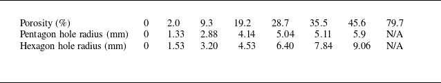


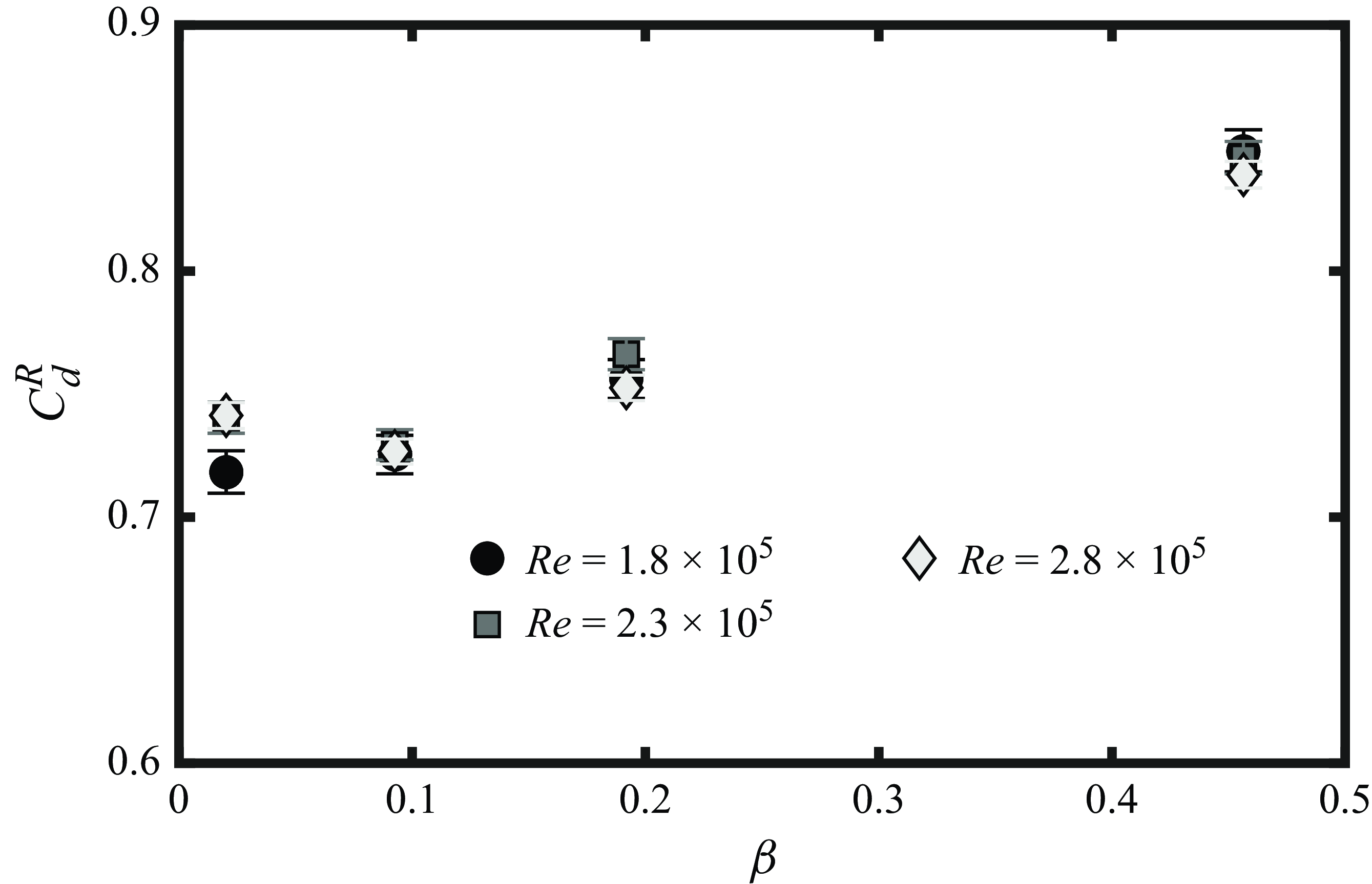


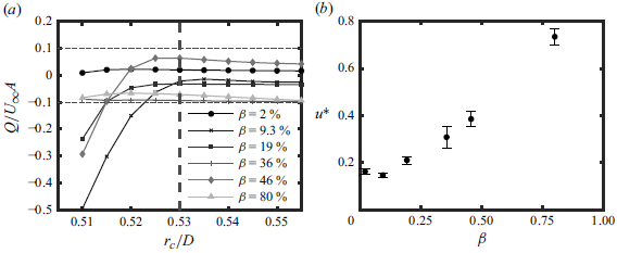


 Open access