


1. Introduction
When small, rigid particles are immersed in a turbulent fluid, diffusible material may be transferred from their surface by convection and diffusion. Often, as is the case for solutes in liquids, the solute diffuses slowly, so that convection is the dominant mechanism of mass transfer away from the particle. Also, the particle is often small in comparison with the Kolmogorov length scale, the smallest dynamically active scale of the turbulence. This phenomenon occurs in an abundance of engineered and natural processes: chemical products are produced by crystallisation, dissolution, fermentation and heterogeneous reactions in liquid–solid suspensions within stirred tanks and fluidised beds (Myerson Reference Myerson2002; Nienow Reference Nienow2006; Crowe et al. Reference Crowe, Schwarzkopf, Sommerfeld and Tsuji2012); planktonic osmotrophs absorb nutrients (Karp-Boss, Boss & Jumars Reference Karp-Boss, Boss and Jumars1996); pollutants leach from microplastics (Seidensticker et al. Reference Seidensticker, Zarfl, Cirpka, Fellenberg and Grathwohl2017); bacteria encounter marine viruses (Guasto, Rusconi & Stocker Reference Guasto, Rusconi and Stocker2012); and breakdown products of marine snow are swept away (Alcolombri et al. Reference Alcolombri, Peaudecerf, Fernandez, Behrendt, Lee and Stocker2021) as they sink through turbulent ocean waters. In these processes, turbulence, inertia and gravity may drive a convective flow around the particle which enhances mass transfer: gravity may cause particles to sink or float (Harriott Reference Harriott1962), inertia may cause particles to slip (Levins & Glastonbury Reference Levins and Glastonbury1972b) and turbulent eddies may convect material away by strain (Batchelor Reference Batchelor1980; Lawson & Ganapathisubramani Reference Lawson and Ganapathisubramani2021). In this paper we ask: for small spherical particles sinking in a turbulent flow, what is the dominant mechanism of mass transfer?
The relative importance of these mechanisms to convective mass transfer, and in some cases their very existence, has been debated extensively in the context of stirred tank reactors (Pangarkar et al. Reference Pangarkar, Yawalkar, Sharma and Beenackers2002; Pangarkar Reference Pangarkar2015). As reviewed by Pangarkar et al. (Reference Pangarkar, Yawalkar, Sharma and Beenackers2002), the proposed mechanisms of mass transfer to small particles fall under three categories: slip velocity theory, penetration theory and Kolmogorov theory. In the slip velocity theory, first proposed by Calderbank & Moo-Young (Reference Calderbank and Moo-Young1961) and later developed by Harriott (Reference Harriott1962), the particle experiences a relative flow due to gravitational settling and its inertial response to turbulent velocity fluctuations. A concentration boundary layer develops whose thickness is controlled by the relative magnitude of diffusion and slip-driven flow and material is swept away from the particle in a single wake. Semi-empirical expressions have subsequently been developed for the particle Sherwood number  ${Sh}$, a dimensionless measure of the mass transfer rate. These expressions are generally of the form (Nienow Reference Nienow1992)
 \begin{equation} {Sh} = 1 + \alpha \textit{Re}_w^\beta {Sc}^\gamma , \end{equation}
where  $\textit{Re} _w = wa/\nu$ is the particle Reynolds number based on the (effective) slip velocity $w$, radius $a$ and kinematic viscosity $\nu$, and ${Sc} = \nu /D$ is the Schmidt number. The exponents $\beta$ and $\gamma$ are sometimes fixed to be $1/2$ and $1/3$, respectively, in order to be consistent with the expected scaling of the concentration boundary layer from boundary layer theory and empirical observations of mass transfer from steadily falling particles (Frössling Reference Frössling1938; Ranz & Marshall Reference Ranz and Marshall1952).
For neutrally buoyant particles, Harriott (Reference Harriott1962) noted this slip velocity must vanish and that mass transfer must be provided by an another mechanism. Harriott (Reference Harriott1962) and later Armenante & Kirwan (Reference Armenante and Kirwan1989) therefore proposed refinements of penetration theory (Higbie Reference Higbie1935), in which mass transfer from the particle is limited by unsteady diffusion under the action of eddies which periodically replenish the concentration boundary layer with fresh fluid. This predicts a mass transfer rate of similar form to (1.1), but with a Reynolds number  $\textit{Re} _\epsilon = a^{4/3}\epsilon ^{1/3}/\nu$ redefined in terms of the energy dissipation rate $\epsilon$. However, the predicted exponents for small spherical particles ( $\beta = 3/4,\gamma = 1/2$) are at variance with the available experimental data (Armenante & Kirwan Reference Armenante and Kirwan1989). Furthermore, the role of the convective flow due to slip (e.g. by sinking) is not incorporated.
An alternative approach for the near-neutrally-buoyant case is offered by Kolmogorov theory (e.g. Calderbank & Moo-Young Reference Calderbank and Moo-Young1961; Levins & Glastonbury Reference Levins and Glastonbury1972a). In this, an effective slip velocity is introduced which is taken to grow with the magnitude of inertial range velocity differences  ${\rm \Delta} u \sim (\epsilon a)^{1/3}$, where $\epsilon$ is the mean dissipation rate and ${\rm \Delta} u$ is the characteristic velocity difference between two points in the flow separated by scale $a$. This also results in a particle Reynolds number $\textit{Re} _\epsilon$ based on the dissipation rate $\epsilon$ for use in (1.1). Whilst the rationale for such a slip velocity is understandable for particles sized in the inertial range, this velocity scale has also been applied to data of particles in the dissipation range, where the rationale is questionable (Armenante & Kirwan Reference Armenante and Kirwan1989). Several other authors (e.g. Levins & Glastonbury Reference Levins and Glastonbury1972b; Ohashi, Sugawara & Kikuchi Reference Ohashi, Sugawara and Kikuchi1981; Armenante & Kirwan Reference Armenante and Kirwan1989) have also formulated an effective slip velocity (on dimensional grounds) based upon the dissipation rate, particle size and viscosity, which is equivalent to the Kolmogorov scaling argument. The specific mechanism of mass transfer is not elucidated in these works and no physical interpretation is given to the effective slip velocity (as emphasised by, for example, Levins & Glastonbury (Reference Levins and Glastonbury1972b) and Armenante & Kirwan (Reference Armenante and Kirwan1989)).
Later, Batchelor (Reference Batchelor1980) introduced a theory of mass transfer to small, suspended solid spheres. The Reynolds number of the motion in the neighbourhood of the particle, associated with either the slip  $\textit{Re} _w$ or the turbulence $\textit{Re} _\epsilon$, is assumed to be small compared with unity. This assumption implies that the particle Stokes number ${St} \sim \textit{Re} _\epsilon ^{3/2} \ll 1$ is also small. This allows the relative flow field to be prescribed as a superposition of a uniform slip velocity, linear velocity gradient and a Stokes perturbation due to the presence of the particle. The concentration boundary layer that develops is analysed with the use of classic asymptotic methods (Leal Reference Leal2012). Because the flow is turbulent, the components of the linear gradient and slip velocity fluctuate in time. Batchelor then argues that at large turbulent Péclet number ${Pe} = a^2\tau _\eta /D = \textit{Re} _\epsilon ^{3/2}{Sc}$, due to the convection-suppression effect (Batchelor Reference Batchelor1979), particle motion due to slip has a negligible effect on the mass transfer rate because the particle rotates isotropically. This convection-suppression mechanism has recently been confirmed in turbulent flows to suppress convective mass transfer by velocity fluctuations occurring on a time scale more rapid than $\tau _\eta {Pe}^{1/3}$ (Lawson & Ganapathisubramani Reference Lawson and Ganapathisubramani2021). In the limit of ${Pe} \rightarrow \infty$, Batchelor concluded that for small spherical particles, the only component of the relative flow field which is persistent upon averaging over time in the particle reference frame is an axisymmetric strain, whose magnitude scales with $1/\tau _\eta$. In the limit of large turbulent Péclet number, this axisymmetric straining flow drives a mass transfer rate like
 \begin{align} {Sh} &= 0.55 {Pe}^{1/3} + O(1) \nonumber\\ &= 0.55{\it Re} _\epsilon^{1/2} {Sc}^{1/3} + O(1). \end{align}
In a reference frame following and rotating with the particle, the solution of concentration boundary layer near the surface asymptotically approaches that of a spherical particle in an axisymmetric extensional strain. This result places empirical correlations based on Kolmogorov theory for small particles on firmer physical grounds, provided that the mechanism of mass transfer due to an effective slip velocity is reinterpreted as mass transfer by the (time-average) ambient straining field.
A striking implication of this analysis is that convection due to slip (e.g. by gravity or inertia) is suppressed at large turbulent Péclet number. Batchelor (Reference Batchelor1980) remarks that the ‘strange consequence’ for sinking particles is that gentle stirring should initially decrease the average mass transfer rate. Batchelor's prediction (1.2) shows reasonable agreement with available experimental data for nearly neutrally buoyant spheres, but conflicts with the observed enhancement of mass transfer for particles where a significant density difference exists (Harriott Reference Harriott1962; Levins & Glastonbury Reference Levins and Glastonbury1972b). The question therefore arises as to how to reconcile the mechanisms of slip and strain in a theory of particle-scale mass transfer.
Recently, we have examined Batchelor's scenario numerically for small, neutrally buoyant spheroids in isotropic turbulence at large but finite turbulent Péclet number (Lawson & Ganapathisubramani Reference Lawson and Ganapathisubramani2021). The motion of spherical and spheroidal tracer particles is simulated in homogeneous, isotropic turbulence and the relative velocity field, which is prescribed by the Lagrangian time history of the linear velocity gradient and Stokes perturbation sampled by the tracer, is used to force the numerical solution of the convection–diffusion equation in the vicinity of the particle. The mass transfer rate predicted by these simulations is found to be in good quantitative agreement with available experimental data for small, spherical particles in turbulence. The results confirm the convection-suppression effect and demonstrate that the concentration boundary layer is unresponsive to velocity fluctuations occurring on a time scale more rapid than  $\tau _d \sim \tau _\eta {Pe}^{1/3}$. The instantaneous mass transfer rate is shown to correlate most strongly with the relative velocity field filtered on this time scale. The conceptual picture that emerges from this analysis is that the instantaneous concentration field near the particle surface is close to the steady-state solution of an equivalent particle subject to the same (time-filtered) relative velocity field. In this interpretation, it is not necessary for slip to make negligible contribution to the mass transfer rate, because a slip velocity may be persistent over shorter times.
In this paper, we examine the mechanisms of mass transfer to small particles sinking in turbulence. In § 2, we revisit the theoretical description given by Batchelor (Reference Batchelor1980) of small spheres exchanging material in a turbulent flow and identify that at large but finite turbulent Péclet number, the sinking ratio  ${Sr} = w_0 \tau _\eta / a$ forms an important control parameter of the mass transfer problem. We also examine qualitatively the properties of the scalar wake in the limits of ${Sr} \ll 1$ and ${Sr} \gg 1$. In § 3, we present a set of flow visualisation experiments designed to identify the mechanism of mass transfer to hydrodynamically small, spherical particles as the sinking ratio is varied. These measurements allow us to reconstruct the instantaneous concentration field in the vicinity of small particles exchanging material with a turbulent flow. This is achieved by visualising the release of dye from small, spherical ion-exchange beads in homogeneous turbulence using shadowgraphic particle tracking and planar laser-induced fluorescence measurements. We describe our methodology and data reduction in §§ 3.1 and 3.2, respectively, and present particle-scale flow visualisations of mass transfer in § 3.3. Our observations confirm that a change in the mechanism of mass transfer occurs when ${Sr} = O(1)$. Based on these experimental insights, we present an extension of our numerical model in § 4 to incorporate the effect of gravity for heavy particles and examine the influence upon the mass transfer rate. After providing a validation of the average transfer rate predicted by our simulations in § 4.2, we quantify the mechanisms of mass transfer in §§ 4.3 and 4.4. The results provide insight into reconciling the two mechanisms in particle-scale mass transfer models. We provide a brief discussion and conclusions in § 5.
2. Theoretical background
In this section, we provide an analytical description of the mass transfer from a dilute suspension of sinking particles. This forms the basis of our numerical model in § 4 and formally identifies  ${Sr}$ as a control parameter in the mass transfer problem. Furthermore, we identify qualitative properties of the scalar wake in the limits of ${Sr} \ll 1$ and ${Sr} \gg 1$ at large but finite ${Pe}$. We base our approach on Batchelor (Reference Batchelor1980), which describes the relative flow field near the particle in terms of a fluctuating slip velocity, turbulent shear and Stokes perturbation. The particle Reynolds number is assumed to be small, so that the Stokes flow approximation is valid. Furthermore, gravitational acceleration is assumed to be strong in comparison with the turbulence.
Let us consider the motion of a small spherical particle of radius  $a$ with position $\boldsymbol {X}(t)$ and velocity $\dot {\boldsymbol {X}}$ in an unsteady turbulent flow field $\boldsymbol {u}(\boldsymbol {x},t)$ under the action of gravitational acceleration $\boldsymbol {g} = g\boldsymbol {e}_z$. The spatial coordinate of the laboratory frame is $\boldsymbol {x}$ and temporal coordinate is $t$. When the particle Reynolds number is sufficiently small, the forces on the particle are prescribed by Stokes flow, and the equation of motion is given by
 \begin{equation} \ddot{\boldsymbol{X}} =\frac{1}{\tau_p}(\boldsymbol{u}(\boldsymbol{X},t) - \dot{\boldsymbol{X}}) + \beta\frac{\mathrm{D}\boldsymbol{u}}{\mathrm{D}t}+ (1-\beta)g\boldsymbol{e}_z + \textrm{Basset history and Saffman lift}, \end{equation}
where  $\tau _p \equiv a^2 / (3\beta \nu )$ is the response time of the particle and $\beta = 3\rho _f/(2\rho _p + \rho _f)$ is the density ratio parameter, in which $\rho _p$ is the density of the particle and $\rho _f$ is the density of the fluid. The Stokes number ${St} = \tau _p/\tau _\eta$ is the measure of the particle response time in comparison with the time scale of the turbulence and implicitly defines the particle size in comparison with the Kolmogorov scale as $a/\eta = (3\beta {St})^{1/2}$. In the small-particle limit ${St} \ll 1$, $\tau _p$ is a small parameter and, regardless of initial conditions, the slip velocity $\boldsymbol {w}_0(\boldsymbol {X},t) = \boldsymbol {u}(\boldsymbol {X},t) - \dot {\boldsymbol {X}}$ exponentially relaxes towards (Ferry & Balachandar Reference Ferry and Balachandar2001)
 \begin{equation} \boldsymbol{w}_0(\boldsymbol{X},t) = (1 - \beta)\left( \frac{\mathrm{D}\boldsymbol{u}}{\mathrm{D}t} - \boldsymbol{g} \right) \tau_p + O(\tau_p^{3/2}). \end{equation}
Therefore, when the gravitational acceleration is much stronger than the material acceleration due to turbulence (i.e.  $\mathrm {D}\boldsymbol {u}/\mathrm {D}t \ll \boldsymbol {g}$), the slip velocity is
 \begin{equation} \boldsymbol{w}_0 = (\beta-1)\boldsymbol{g}\tau_p = w_0\boldsymbol{e}_z \end{equation}
to leading order in  $\tau _p$. This is simply the settling velocity in quiescent flow and becomes independent of tracer position $\boldsymbol {X}$ and time $t$. The fluid acceleration is a small-scale quantity which scales with the Kolmogorov scale $a_\eta = (\epsilon ^3/\nu )^{1/4}$ (Voth et al. Reference Voth, La Porta, Crawford, Alexander and Bodenschatz2002), so (2.3) is valid for small Froude number ${Fr} = a_\eta / g \ll 1$. This restricts the choice of ${Sr}, {St}$ and the density ratio $\beta$ via the relationship
 \begin{equation} {Sr} = \frac{|1 - \beta|}{\sqrt{3\beta}} \frac{{St}^{1/2}}{{Fr}}. \end{equation}
Thus if we fix  ${St}$ and ${Fr}$ to be much smaller than unity, the density ratio $\beta$ essentially controls the sinking ratio. These joint assumptions are restrictive but relevant to our motivating examples. For instance, a quick calculation based on Karp-Boss et al. (Reference Karp-Boss, Boss and Jumars1996) shows that marine diatoms absorb nutrients in turbulent environments with ${St} \ll 1$ and ${Fr} \ll 1$. Similarly, a common design requirement for bioreactors is for cells to be much smaller than the Kolmogorov scale to avoid shear-induced damage (i.e. ${St} \ll 1$) (Nienow Reference Nienow2006), which typically results in small Froude numbers also.
The relative velocity field in the frame co-moving with the tracer  $\boldsymbol {w}(\boldsymbol {r},t) = \boldsymbol {u}(\boldsymbol {X}+\boldsymbol {r},t) - \dot {\boldsymbol {X}}$ is given as a superposition of the slip velocity, the ambient linear velocity gradient surrounding the particle plus a perturbation due to the Stokes flow surrounding the particle. This is
 \begin{equation} \boldsymbol{w}(\boldsymbol{r},t) = \boldsymbol{w}_0 + \boldsymbol{\mathsf{G}}(\boldsymbol{X},t)\boldsymbol{r} + \boldsymbol{w}'(\boldsymbol{r},t), \end{equation}
where  ${\mathsf{G}}_{ij} = \partial u_i/\partial x_j$ is the velocity gradient tensor sampled at the particle position and $\boldsymbol {w}'(\boldsymbol {r},t)$ is the Stokes perturbation due to the presence of the particle. For an infinitesimal particle, this Stokes perturbation is expressed as a function of the instantaneous slip velocity $\boldsymbol {w}_0$, gradient $\boldsymbol {G}$ and the boundary condition at the particle surface $|\boldsymbol {r}|=a$ (Kim & Karrila Reference Kim and Karrila1991).
As the particle translates, it is also free to rotate with angular velocity  $\boldsymbol {\varOmega } = \boldsymbol {\omega }/2$ prescribed by the ambient vorticity $\boldsymbol {\omega }$ (Jeffery Reference Jeffery1922). Therefore, in the coordinate system $\boldsymbol {y}$ co-moving and co-rotating with the particle, we have $\boldsymbol {r} = \boldsymbol{\mathsf{R}}\boldsymbol {y}$, where the orientation of the body frame $\boldsymbol{\mathsf{R}}$ evolves as
 \begin{equation} \frac{\mathrm{d}\boldsymbol{\mathsf{R}}}{\mathrm{d}t} = \left[\boldsymbol{\varOmega}\right]_\times \boldsymbol{\mathsf{R}}. \end{equation}
The ambient velocity field  $\boldsymbol {v}(\boldsymbol {y},t)$ in this co-rotating system is therefore
 \begin{align} \boldsymbol{v}(\boldsymbol{y},t) &= \boldsymbol{\mathsf{R}}^\textrm{T}\boldsymbol{w} + \dot{\boldsymbol{\mathsf{R}}}^\textrm{T}\boldsymbol{r}, \nonumber\\ &= \boldsymbol{v}_0 + \boldsymbol{\mathsf{E}}\boldsymbol{y} + \boldsymbol{v}'(\boldsymbol{y},t), \end{align}
where we have introduced  $\boldsymbol {v}_0 = \boldsymbol{\mathsf{R}}^\textrm {T}\boldsymbol {w}_0$ as the settling velocity in the co-rotating frame, $\boldsymbol{\mathsf{E}} = \boldsymbol{\mathsf{R}}^\textrm {T}(\boldsymbol{\mathsf{G}} - [\boldsymbol {\varOmega }]_\times )\boldsymbol{\mathsf{R}}$ is the rate-of-strain tensor in this frame and $\boldsymbol {v}'(\boldsymbol {y},t) = \boldsymbol{\mathsf{R}}^\textrm {T}\boldsymbol {w}'$ is the Stokes perturbation in the rotating frame. We note that in this co-rotating frame, the fluid is at rest at the particle surface $|\boldsymbol {y}| = a$.
The convection–diffusion equation can now be written in dimensionless form, normalising by the particle radius  $a$ and Kolmogorov timescale $\tau _\eta$ (Leal Reference Leal2012; Lawson & Ganapathisubramani Reference Lawson and Ganapathisubramani2021):
 \begin{equation} \frac{\partial\theta}{\partial {t}^{{\star}}} + {\boldsymbol{v}}^{{\star}}\boldsymbol{\cdot} \boldsymbol{\nabla}_\star\theta = \frac{1}{{Pe}}\nabla_\star^2 \theta, \end{equation}
where  $\theta ({\boldsymbol {y}}^{\star },t)$ is the (dimensionless) concentration of the solute. Our convention is that terms written with a superscript $^\star$ (e.g. ${\boldsymbol {v}}^{\star } = \boldsymbol {v}\tau _\eta /a, {\boldsymbol {y}}^{\star } = \boldsymbol {y}/a$) have been non-dimensionalised with $\tau _\eta$ and $a$. The turbulent Péclet number is defined as ${Pe} \equiv a^2/D\tau _\eta$ for solute diffusion coefficient $D$. We distinguish this from the quiescent settling Péclet number ${Pe}_w \equiv a w_0/D = {Pe}{Sr}$. We consider a uniform concentration boundary condition:
 \begin{equation} \left.\begin{matrix} \theta({\boldsymbol{y}}^{{\star}}, t) = 1 & |{\boldsymbol{y}}^{{\star}}| = 1 \\ \theta({\boldsymbol{y}}^{{\star}}, t) = 0 & |{\boldsymbol{y}}^{{\star}}| \rightarrow \infty .\\ \end{matrix}\right\} \end{equation}
This corresponds to a uniform (dimensional) concentration at the particle surface  $C_1$ and uniform concentration far from the particle $C_0$ with $\theta = (C(\boldsymbol {y},t) - C_0)/(C_1 - C_0)$. The Sherwood number, the non-dimensional measure of the solute flux $Q$, is defined as
 \begin{equation} {Sh} = \frac{Q}{4{\rm \pi} r D(C_1-C_0)} ={-}\frac{1}{4{\rm \pi}{Pe}} \iint_{|{\boldsymbol{y}}^{{\star}}|=1} \boldsymbol{\nabla}_\star\theta \boldsymbol{\cdot}\mathrm{d}\boldsymbol{S}. \end{equation}
Thus,  ${Sh} = 1$ for a sphere with mass transfer by diffusion alone.
Let us examine the magnitude of the terms in the non-dimensionalised relative velocity field:
 \begin{equation} {\boldsymbol{v}}^{{\star}}({\boldsymbol{y}}^{{\star}},{t}^{{\star}}) = \underbrace{\frac{\boldsymbol{v}_0\tau_\eta}{r}}_{O(w_0\tau_\eta/a)} + \underbrace{{\boldsymbol{\mathsf{E}}}^{{\star}}{\boldsymbol{y}}^{{\star}}}_{O(y/a)} + \boldsymbol{v}^{\prime\star}({\boldsymbol{y}}^{{\star}},{t}^{{\star}}). \end{equation}
The slip velocity has magnitude  $w_0 \tau _\eta /a$, although its orientation changes with time as the particle rotates. Near the particle, the influence of the linear velocity gradient is $O(1)$, and the Stokes perturbation is comparable to the sum of these terms. The sinking ratio ${Sr} \equiv w_0\tau _\eta /a$ therefore forms a natural control parameter of the problem, in addition to the turbulent Péclet number, the Stokes number and density parameter.
Batchelor (Reference Batchelor1980) argued that in the limit of  ${Pe} \rightarrow \infty$, the solution of (2.8) near the particle surface asymptotically approaches the solution of
 \begin{equation} \widetilde{{\boldsymbol{v}}^{{\star}}}\boldsymbol{\cdot} \boldsymbol{\nabla}\theta = \frac{1}{{Pe}}\nabla^2 \theta , \end{equation}
where
 \begin{equation} \widetilde{{\boldsymbol{v}}^{{\star}}}({\boldsymbol{y}}^{{\star}},{t}^{{\star}}) = \frac{1}{{\tau_f}^{{\star}}} \int_{-{\tau_f}^{{\star}}}^{0} {\boldsymbol{v}}^{{\star}}({\boldsymbol{y}}^{{\star}},{t}^{{\star}}+t')\,\mathrm{d}t' \end{equation}
is the relative velocity field averaged over a long time  ${\tau _f}^{\star }$. This is justified on the basis that the concentration boundary layer becomes insensitive to velocity fluctuations that are more rapid than $\tau _\eta {Pe}^{1/3}$ due to the convection-suppression effect (Batchelor Reference Batchelor1979; Lawson Reference Lawson2021). Taking the average in the limit ${\tau _f}^{\star } \rightarrow \infty$, Batchelor (Reference Batchelor1980) concluded that the average convective contribution due to slip in (2.11) vanishes, because the particle orientation is isotropic in the large-time limit. Therefore, in Batchelor's analysis, the sinking ratio does not appear as a control parameter. However, for neutrally buoyant spheroids, we have empirically shown shown that at large but finite ${Pe}$, the solution of (2.8) is best approximated by (2.12) when the time scale is chosen ${\tau _f}^{\star } \sim {Pe}^{1/3}$ (Lawson & Ganapathisubramani Reference Lawson and Ganapathisubramani2021). Under this hypothesis, it is therefore still possible for slip to contribute to the convective mass transfer, because $\widetilde {{\boldsymbol {v}_0}^{\star }}$ does not vanish when averaging over a finite time interval.
Figures 1(a) and 1(b) illustrate the topology of the concentration field for solute transfer from a spherical particle in steady, axisymmetric strain, i.e.  ${Sr} \ll 1$. Solute is advected away from the particle by convection due to strain in a thin, symmetric, line-like (figure 1a) or sheet-like (figure 1b) wake, depending upon the direction of the strain along the symmetry axis. On the other hand, under uniform slip ${Sr} \gg 1$ (figure 1c), solute streams from the particle along a single, line-like wake. Therefore, the mechanism of the mass transfer and the topology of the wake are predicted to be qualitatively different at ${Sr} \ll 1$ and ${Sr} \gg 1$.

Figure 1. Illustration of solute transfer from a small, spherical particle at large Péclet number under steady (a) extensional axisymmetric strain, (b) compressive axisymmetric strain and (c) uniform flow.
3. Laboratory experiments
In this section, we present a set of flow visualisation experiments designed to identify the mechanism of mass transfer to hydrodynamically small, spherical particles as the sinking ratio is varied. The basic principle is to load spherical ion-exchange beads with a fluorescent anionic dye (fluorescein) which is released upon contact with a sodium chloride solution. We then track the motion of particles in homogeneous turbulence using high-speed shadowgraph imaging and visualise the dye release using planar laser-induced fluorescence (PLIF). Resultant three-dimensional (3-D) reconstructions of the concentration field are then analysed to statistically characterise the concentration wake as a function of the sinking ratio.
3.1. Experimental methodology
Here, we describe our experimental set-up and our procedure for tracking particles and reconstruct the concentration field surrounding the particle. Our experimental set-up is illustrated in figure 2(a). It consists of three main components: a randomly stirred mixing tank to generate homogeneous turbulence, dye-laden particles and a combined shadowgraph and PLIF imaging set-up to track particles to obtain particle-scale measurements of dye release. We now describe each.

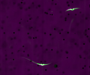
Figure 2. (a) Photograph of experimental apparatus, illustrating: impeller-stirred mixing tank; high-speed shadowgraph imaging arrangement including cameras, prisms and collimated backlight sources; and PLIF laser, optics and sheet. (b) Visualisation of the concentration boundary layer and wake around fine particles in turbulence, showing PLIF image (green channel) and shadowgraph image of particle (purple channel). Supplementary movies 1 and 2 available at https://doi.org/10.1017/jfm.2022.998 show sample PLIF/shadowgraph video sequences.
3.1.1. Mixing tank
To generate homogeneous turbulence in our laboratory, we use the randomly stirred mixing tank facility described in Lawson & Ganapathisubramani (Reference Lawson and Ganapathisubramani2022). We provide a brief description here. It consists of a  $45\,\textrm {l}$ capacity transparent poly(methyl methacrylate) (PMMA) tank (internal dimensions $500\,\textrm {mm} \times 300\,\textrm {mm} \times 300\,\textrm {mm}$) with a removable lid and $32$ pitched-blade impellers, driven by independently controlled stepper motors. These are spaced $75\,\textrm {mm}$ apart on a $4 \times 4$ square grid and are mounted through the side-wall of the tank. The lid of the tank is removable; the tank is filled with water to a level slightly above the lid. Between experimental runs, the water was drained and refilled twice to ensure the tank was clean and free of dye. The water temperature was not regulated and varied between $T = 20$ and $21\,^\circ \textrm {C}$. Based on this temperature measurement, we obtain the mass density $\rho _f$, kinematic viscosity $\nu$ and dynamic viscosity $\mu$ of the water from literature data (Lide Reference Lide2013).
To create unsteady forcing, we implement the ‘sunbathing’ algorithm of Variano & Cowen (Reference Variano and Cowen2008), which has been widely used in jet-stirred mixers (Variano & Cowen Reference Variano and Cowen2008; Bellani & Variano Reference Bellani and Variano2014; Carter et al. Reference Carter, Petersen, Amili and Coletti2016; Pérez-Alvarado, Mydlarski & Gaskin Reference Pérez-Alvarado, Mydlarski and Gaskin2016; Esteban, Shrimpton & Ganapathisubramani Reference Esteban, Shrimpton and Ganapathisubramani2019). We drive the impellers at a fixed rotation rate  $f_I$ whilst randomly reversing the direction of motion. Each impeller switches between spinning clockwise for a time $\tau _F$ and then anticlockwise for a time $\tau _R$. Following Variano & Cowen (Reference Variano and Cowen2008), the durations of forward thrust $\tau _F \sim \mathcal {N}(\mu _F, \mu _F/3)$ and reverse thrust $\tau _R \sim \mathcal {N}(\mu _R, \mu _R/3)$ are drawn from a normal distribution (clipped at zero) with means $\mu _F, \mu _R$ and standard deviations $\mu _F/3, \mu _R/3$. Following Lawson & Ganapathisubramani (Reference Lawson and Ganapathisubramani2022), we choose a source fraction $\phi = \mu _F / (\mu _F + \mu _R) = 0.25$ and a forcing period $\mu _F + \mu _R = 32\,\textrm {s}$, which are chosen to optimise the intensity and homogeneity of the turbulence.
We have previously characterised the turbulence generated in our mixing tank using particle image velocimetry (PIV) (Lawson & Ganapathisubramani Reference Lawson and Ganapathisubramani2022). The mean flow at the centre of the tank is weak, accounting for around 1 %–4 % of the total kinetic energy in the  $75\,\textrm {mm} \times 75\,\textrm {mm} \times 75\,\textrm {mm}$ region near the geometric centre. Here, the flow is dominated by nearly isotropic turbulent velocity fluctuations, which have a characteristic magnitude $u'$ and are homogeneous to within the standard statistical uncertainty ( ${\pm }2.2\,\%$) of our PIV measurements. The mean dissipation rate $\epsilon$ at the centre of the tank was obtained from fits of the second-order structure function. Additionally, using the large-eddy PIV method (De Jong et al. Reference De Jong, Cao, Woodward, Salazar, Collins and Meng2009), we have found the spatial distribution of the mean energy dissipation rate is homogeneous to within ${\pm }41\,\%$ of the spatial average near the centre of the tank. The integral autocorrelation length scale in this region is around 58–70 mm. We conclude that the recent Lagrangian history of the particles observed in our measurement volume approximates that found in homogeneous, isotropic turbulence.
3.1.2. Dye-laden particles
To create spherical dye-laden particles, we load sodium fluorescein dye (Sigma Aldrich) onto commercially available anion-exchange resin beads (Dowex  $1{\text{X}}2$, Fischer Scientific). The beads, which are supplied in $\textrm {Cl}^-$ form, undergo a reversible reaction as
 \begin{equation} \textrm{R}\textrm{Cl} + \textrm{Na}\textrm{Fl} \rightleftharpoons \textrm{R}\textrm{Fl} + \textrm{Na}\textrm{Cl}. \end{equation}
In a typical procedure, we prepare  $100\,\textrm {ml}$ of a $0.2\,\textrm {M}$ solution of sodium fluorescein to which $15\,\textrm {g}$ of ion-exchange beads is added under stirring. This loading of dye is close to the capacity of the ion-exchange beads and the dye solution is visibly depleted afterwards. We have observed that sodium fluorescein is not absorbed well onto resin beads in $\textrm {OH}^-$ form.
Relevant physical properties of the dye-laden particles are presented in table 1. The mean particle radius  $\left \langle a \right \rangle$ and standard deviation $\sigma _a$ were obtained by processing microscope images taken at a resolution of $400\,\textrm {px}\,\textrm {mm}^{-1}$ using a Hough-transform circle-detection routine. Statistics were based upon samples of 381 (50–100 mesh), 1350 (100–200 mesh) and 5152 (200–400 mesh) particles. While the larger 50–100 mesh particles exhibited little variation in size, the smallest 200–400 mesh particles had a relatively large coefficient of variation $\sigma _a/\left \langle a \right \rangle$ of around $24\,\%$. Particle density was measured in triplicate using a $5\,\textrm {ml}$ pycnometric flask and an analytical balance with $10\,\textrm {mg}$ resolution. The quiescent settling velocity in water at $20\,^\circ \textrm {C}$ was calculated from
 \begin{equation} w_0 = \sqrt{\frac{g \left\langle a \right\rangle}{3 C_D } \frac{\rho_p - \rho_f}{\rho_f}} \end{equation}
based on the empirical drag coefficient relation
 \begin{equation} C_D = \frac{24}{{\it Re} _{w}} \left( 1 + 0.1315 {\it Re} _{w}^{0.82 - 0.05\log_{10} {\it Re} _{w}} \right) , \end{equation}
which is applicable in the Reynolds number range  ${\it Re} _{w} = 0.01$– $20$ (Clift, Grace & Weber Reference Clift, Grace and Weber1978).
Table 1. Properties of fluorescent dye-laden particles. Uncertainty in particle density is  ${\pm }2\,\textrm {kg}\,\textrm {m}^{-3}$. The quiescent settling velocity $w_0$ in water at $20\,^\circ \textrm {C}$ was calculated based on the particle density $\rho _p$ and mean radius $\left \langle a \right \rangle$ using (3.2).

3.1.3. Shadowgraph and PLIF imaging
The combined shadowgraph and PLIF imaging set-up is shown in figure 2(a). In this, shadowgraph particle images are recorded by three Phantom v641 high-speed cameras, whilst PLIF images are recorded by the central camera only using illumination provided by a thin, continuous wave laser sheet. The shadowgraph and PLIF images are interleaved by time-multiplexing: pulsed backlight illumination is provided every other frame, so that frames recorded by the central camera alternate between PLIF and PLIF with shadows. Figure 2(b) shows an example of a sequential shadowgraph/PLIF image pair: particle shadows are visible over a wide depth of field, allowing for particle tracking, whilst dye fluorescence is only observed in the plane of the laser sheet.
Three coplanar cameras are used for 3-D particle tracking. The central camera is oriented normal to the laser sheet, whilst the side cameras view the flow near the centre of the tank at  ${\pm }30^\circ$ to the sheet normal. A set of 3-D-printed prisms with $2.5\,\textrm {mm}$ thick acrylic windows allow the side cameras to view the flow without distortion across the air–PMMA–water interface. The shadowgraph backlight is provided by pulsed blue LEDs (Osram Golden DRAGON Plus), which are collimated by Sigma $105\,\textrm {mm}$ lenses to evenly illuminate a small $13.7\,\textrm {cm}^3$ measurement volume at the centre of the tank. Particle shadows are imaged using a Nikon f/2.8 200 mm Macro lens, which achieves an optical magnification of almost $1:1$. The spatial resolution in the PLIF measurement plane is $11.4\,\mathrm {\mu }\textrm {m}\,\textrm {px}^{-1}$. This illumination set-up means that the depth of field of the shadowgraph image is set by the collimation of the backlight, whereas the depth of field of PLIF imaging is set by the central camera's aperture ( $f_\# = 5.6$). To exclude the laser signal from the side cameras, we use a narrower aperture ( $f_\# = 11$) so that any reflected light or fluorescent emission is very dim in comparison to the backlight.
Continuous-wave laser illumination is provided by a  $1.1\,\textrm {W}$, Coherent Genesis MX laser at $514\,\textrm {nm}$. This choice of excitation wavelength is suboptimal for sodium fluorescein, which has peak excitation at $494\,\textrm {nm}$, but provides satisfactory excitation of fluorescence. The beam is formed into a narrow laser sheet by a $-10\,\textrm {mm}$ focal length cylindrical lens and $350\,\textrm {mm}$ spherical lens. The near-Gaussian beam quality ( $M^2 = 1.06$) allows us to achieve a diffraction-limited beam waist of $w \approx 220\,\mathrm {\mu }\textrm {m}$. Because the PLIF excitation wavelength is close to the emission wavelength, we did not use a low-pass cut-off filter to isolate the fluorescence emission. Instead, we minimise the transmission of specular reflections from particles using a linear polariser on the central camera. Image acquisition is synchronised across cameras at a frame rate $f_s$ with an exposure time of $250\,\mathrm {\mu }\textrm {s}$, which provided an acceptable compromise between motion blur and fluorescence signal intensity. The backlight pulse is much shorter $({\le }35\,\mathrm {\mu }\textrm {s})$ so that position uncertainty due to motion blur of shadows is negligible. The frame rate was chosen to obtain a root-mean-square particle displacement of around 5–13 px between shadowgraph frames.
Calibration of the camera arrangement was performed using a  $12\,\textrm {mm} \times 16\,\textrm {mm}$ chessboard calibration target with $1\,\textrm {mm}$ squares laser-printed at 1200 dpi onto transparency film and transferred to a glass microscope slide. This was traversed across the measurement volume using a translation stage at $z = -10$ to $10\,\textrm {mm}$ at $2\,\textrm {mm}$ intervals. We then obtain a calibration using a standard pinhole camera model. Since the objective of these measurements is to visualise rather than quantify the scalar field, we did not calibrate fluorescence intensity against the dye concentration. However, we have confirmed with spectrophotometric measurements that the equilibrium dye concentration at the particle surface is $O(\mathrm {\mu }\textrm {mol}\,\textrm {l}^{-1})$, so that the fluorescence emission is in the linear regime.
3.2. Particle tracking and wake reconstruction
Table 2 summarises the experimental conditions tested. From our previous PIV characterisation (Lawson & Ganapathisubramani Reference Lawson and Ganapathisubramani2022) and the particle properties in table 1, we compute the particle Stokes number  ${St}$, turbulent Péclet number ${Pe}$, sinking ratio ${Sr}$ and size relative to the Kolmogorov scale. Although the turbulent Péclet number is not controlled for in our experiments, the values are well within the convection-dominated regime ( ${Pe} \gg 1$). It can be seen that the particles in our experiments are comparable to or smaller than the smallest dynamically active motions of the turbulent flow. For all cases, the characteristic turbulent acceleration $a_\eta = (\epsilon ^3/\nu )^{1/4}$ is at least one order of magnitude smaller than the strength of gravitational acceleration, so slip due to turbulent acceleration is negligible. Furthermore, for the two smallest classes of particles, ${St} \ll 1$. By varying the turbulence intensity, we varied the sinking ratio ${Sr}$ by an order of magnitude over the range in which the transition in mass transfer mechanism is expected to occur. For each condition, we obtained time series of 2738 (5000 at 2.4 kHz frame rate) shadowgraph and PLIF images, corresponding to between 1.9 and 6.8 s of turbulent motion, equivalent to approximately 1.3–3.2 integral time scales.
Table 2. Summary of experimental conditions.

Lagrangian particle tracking was performed using an in-house code based on Lawson et al. (Reference Lawson, Bodenschatz, Lalescu and Wilczek2018). This implements a low-density, predictor–corrector particle tracking algorithm following Ouellette, Xu & Bodenschatz (Reference Ouellette, Xu and Bodenschatz2006). The main difference is in particle image registration. Shadowgraph images are first levelised against a white image obtained from the  $95$th brightness percentile on a per-pixel basis. Subsequently, particle centres are identified using a Hough circle transform. Existing particle tracks are extrapolated linearly based on the last two frames and matched to the nearest corresponding particle centres (within a search radius of $20\,\textrm {px}$) and satisfying a triangulation tolerance ( $5\,\textrm {px}$). New tracks are initiated by triangulating unmatched particles and are extrapolated using a nearest-neighbour interpolation of the particle velocity field, with a larger search tolerance. Tracks are terminated if a suitable match is not found or if matching is ambiguous.
We apply Taylor's frozen flow hypothesis to reconstruct the scalar field in the vicinity of particles as they cross the laser sheet. In order to do this, we identify when particles cross the laser sheet based on their position and a calibrated model of the laser sheet plane. This plane is identified using the procedure illustrated in figure 3. When particles cross the laser sheet, we observe a sharp increase in their brightness due to their fluorescence as well as specular reflections, as shown in figure 3(a). We identify a set of crossing events based on a threshold, which define a set of points known to lie upon the laser sheet plane, as illustrated in figure 3(b). We use a robust fitting procedure to fit a plane to these points.

Figure 3. Identification of the laser sheet plane from particle trajectories. (a) An example of time-series measurements of particle brightness, showing the identification of particles which cross the laser sheet. (b) A 3-D reconstruction of the laser sheet plane (green), based on the position of identified crossings (black circles) of particle trajectories. Particle trajectories have been coloured according to their brightness. The white dotted line indicates the particle radius.
To reconstruct the 3-D scalar field, we identify the time  $t_0$ when a particle trajectory $\boldsymbol {X}(t)$ crosses the laser sheet plane $\boldsymbol {X}(t_0)\boldsymbol {\cdot}\boldsymbol {e}_n + c = 0$. The PLIF images $I_{2D}(\boldsymbol {S}+\boldsymbol {s}, t)$ are then sampled in the vicinity of the projected position of the particle $\boldsymbol {S} = \boldsymbol {P}(\boldsymbol {X})$, where $\boldsymbol {s}$ is the two-dimensional (2-D) image coordinate relative to the particle centre and $\boldsymbol {P}(\boldsymbol {x})$ represents the projection operation from 3-D object space to the 2-D image space of the camera. Images are sampled over $\pm 5$ frames around each crossing event. Combined with the constraint that the fluorescence is emitted in the laser sheet plane, this allows us to reconstruct 11 planar slices of the scalar field $I_j(\boldsymbol {r})$ in the co-moving particle frame (2.5) for each crossing event $j$.
$j$.
3.3. Results
Some representative examples of 3-D reconstructions of the scalar field in the co-moving particle frame are illustrated in the top row of figure 4. In these experiments, the particle type (and therefore the sinking speed) is held constant, whilst the dissipation rate (i.e. the characteristic rate of turbulent strain) is varied by changing the impeller speed. We observe that when the sinking ratio  ${Sr} \gg 1$ (as in figure 4a), particles tend to have a single wake which is approximately aligned with the direction of sinking ( $r_2$ axis). This indicates that slip is the dominant mechanism of convective mass transfer. We note, however, that the wake is not perfectly aligned with the direction of gravitational acceleration. When ${Sr} \ll 1$, the typical wake topology changes. Instantaneously, we observe examples of sheet-like (figure 4b) and line-like (figure 4c) distributions of dye around the particle, which indicate that strain is the dominant mechanism of convective mass transfer. The bottom row of figure 4 shows the reconstructions projected in the laser sheet plane, i.e. averaged over the depth coordinate $r_3$. In these, we see that sheet-like or line-like distributions of dye are projected with two wakes, whereas only one wake is visible in the slip-dominated case. As can be observed in supplementary movies 1 and 2, these asymmetric single-wake or symmetric double-wake structures are common in these limiting cases.

Figure 4. Reconstructions of the instantaneous scalar field in a co-moving frame around sinking, 100–200 mesh particles embedded in homogeneous turbulence: (a)  $f_I = 1\,\textrm {Hz}, {Sr} = 8.19$; (b,c) $f_I = 6\,\textrm {Hz}, {Sr} = 0.34$. Upper panels show 3-D reconstructions of the scalar field. Lower panels show the 2-D projection of the scalar field as the particle transits the laser sheet. Sample video sequences of cases (a) and (b,c) are shown in supplementary movies 1 and 2, respectively. Gravitational acceleration is aligned with the $-r_2$ direction (particles sink in the direction of $r_2$ decreasing).
To characterise the average topology of the surrounding wake in the co-moving frame, we evaluated the ensemble-average 2-D projection of the reconstructed scalar field  $\left \langle I_j(\boldsymbol {r}) \right \rangle _{z}$ for all crossing events $j$. This is shown in figure 5. We observe that, when the sinking ratio is large (figure 5a–c), there is a clear signature of the concentration wake created by gravitational slip. However, as the sinking ratio is decreased, the mean distribution of dye around the particle becomes more isotropic. This effect is most pronounced at the smallest sinking ratio (e.g. figure 5j,k). This demonstrates that the mass transfer cannot be explained by gravitational settling alone when the sinking ratio is $O(1)$ or smaller: turbulent shear, acceleration and strain may all act to isotropise the mean distribution of scalar around the particle. Evident in figure 5 is also an artefact of our imaging method: images are dimmer on the right-hand side where a shadow has been cast by the particle. Due to the background subtraction we apply, which subtracts the average intensity over the $r_1$ direction, the signal of the unshadowed portion of the laser sheet is also artificially increased.

Figure 5. Two-dimensional projections of the mean scalar field around sinking particles embedded in homogeneous turbulence, evaluated in the laboratory-aligned co-moving frame: (a,d,g,j) 200–400 mesh ( $\left \langle a \right \rangle =50\,\mathrm {\mu }\textrm {m}$), $\epsilon = 15\unicode{x2013}8690\,\textrm {mm}^2\,\textrm {s}^{-2}$; (b,e,h,k) 100–200 mesh ( $77\,\mathrm {\mu }\textrm {m})$, $\epsilon = 15\unicode{x2013}8690\,\textrm {mm}^2\,\textrm {s}^{-2}$; (c,f,i) 50–100 mesh ( $190\,\mathrm {\mu }\textrm {m}$), $\epsilon = 210\unicode{x2013}8690\,\textrm {mm}^2\,\textrm {s}^{-2}$. The dashed white circle shows $r = 2\left \langle a \right \rangle$.
To identify a change in the mechanism of mass transfer, we repeat our analysis in a coordinate system aligned with the particle wake. To do this, we define a polar coordinate system  $(r,\theta )$ for the projected scalar field $I_{2D}(r,\theta ) = \left \langle I(\boldsymbol {r}) \right \rangle _z$ such that $r_1 = r\cos \theta, r_2 = r\sin \theta$. We identify the angle $\theta _{m,i}$ at which $I_{2D}(2\left \langle a \right \rangle,\theta )$ is maximised, i.e. we identify the instantaneous orientation of the wake at the radius shown in figure 5. We then evaluate the average scalar field in this in a new, wake-aligned relative coordinate system $(r,\theta ')$, where $\theta '=\theta -\theta _{m,i}$ and $r_1' = r\cos \theta ', r_2' = r\cos \theta '$. The result is shown in figure 6. We observe that, when the sinking ratio is large (e.g. figure 6a–f), the average wake-aligned field shows a single wake. However, when the sinking ratio is small (e.g. figure 6g,j,k), a second concentration wake appears on the opposite side of the particle. This is consistent with the expected distribution of scalar for particles with strain-dominated mass transfer (see figures 9 and 4). A second wake structure is not observed on average for the largest 50–100 mesh particles with ${\it Re} _w > 1$, but this may be because our experiments do reach sufficiently small ${Sr}$ (compare e.g. figure 6h,i). Therefore, our laboratory flow visualisations confirm a change in the mechanism of mass transfer for particles in the Stokes regime ( ${\it Re} _w < 1$) as the sinking ratio is varied.

Figure 6. Two-dimensional projections of the mean scalar field around sinking particles embedded in homogeneous turbulence, evaluated in the wake-aligned co-moving frame: (a,d,g,j) 200–400 mesh ( $\left \langle a \right \rangle =50\,\mathrm {\mu }\textrm {m}$), $\epsilon = 15\unicode{x2013}8690\,\textrm {mm}^2\,\textrm {s}^{-2}$; (b,e,h,k) 100–200 mesh ( $77\,\mathrm {\mu }\textrm {m})$, $\epsilon = 15\unicode{x2013}8690\,\textrm {mm}^2\,\textrm {s}^{-2}$; (c,f,i) 50–100 mesh ( $190\,\mathrm {\mu }\textrm {m}$), $\epsilon = 210\unicode{x2013}8690\,\textrm {mm}^2\,\textrm {s}^{-2}$. The dashed white circle shows $r' = 2\left \langle a \right \rangle$.
4. Numerical simulations
Our experiments have confirmed that a transition in the mechanism of mass transfer occurs as the sinking ratio is varied. However, they do not allow us to quantify the relative contributions of convection due to strain and slip. In this section, we extend the approach developed in Lawson & Ganapathisubramani (Reference Lawson and Ganapathisubramani2021) to simulate the mass transfer from a dilute suspension of sinking particles by incorporating a slip velocity. This will allow us to quantify in detail the relative roles of the two mechanisms. The basic idea is to force (2.8) using the Lagrangian time history of the relative velocity field perceived by sinking point-particles a in direct numerical simulation of homogeneous, isotropic turbulence. The convection–diffusion problem is solved numerically on a boundary-fitted domain in a reference frame co-moving and co-rotating with the particle. The grid is sufficiently refined to resolve the development of the concentration boundary layer near the particle surface. The domain is truncated far from the particle and the inflow boundary condition there models incoming fluid as uncontaminated, so that the turbulence effectively provides a continuous supply of fresh fluid. This method retains the advantage of particle-resolved direct numerical simulation (Feng & Michaelides Reference Feng and Michaelides2009; Deen et al. Reference Deen, Peters, Padding and Kuipers2014) that the concentration boundary layer surrounding the particle is resolved, but disregards larger-scale mixing and turbulent transport.
4.1. Numerical methodology
The numerical procedure to implement the model is similar to that of Lawson & Ganapathisubramani (Reference Lawson and Ganapathisubramani2021). We summarise the details here only briefly. The trajectories of particles sinking in homogeneous, isotropic turbulence at  $R_\lambda = 433$ are obtained from the Johns Hopkins Turbulence Database (Li et al. Reference Li, Perlman, Wan, Yang, Meneveau, Burns, Chen, Szalay and Eyink2008). Ensembles of $1000$ Lagrangian particles are uniformly seeded throughout the simulation domain at time $t=0$ and their trajectories are integrated as
 \begin{equation} \dot{\boldsymbol{X}} = \boldsymbol{u}(\boldsymbol{X}(t), t) + \boldsymbol{w}_0, \end{equation}
where the settling velocity is given by (2.3). Equation (4.1) is integrated over the duration of the simulation  $T_{sim} = 10.056$ using a second-order Runge–Kutta scheme with a time step ${{\rm \Delta} t} = 0.002 \approx 0.047\tau _\eta$, corresponding to the time resolution of the database. The velocity and velocity gradient are interpolated from the database at the tracer position using a fourth-order Lagrange polynomial interpolation. This yields a time series of the local velocity gradient $\boldsymbol{\mathsf{G}}(\boldsymbol {X},t_i)$ at $i = 0 \ldots 5028$ times $t_i = i{\rm \Delta} t$. The orientation of the body frame $\boldsymbol{\mathsf{R}}(t)$ (2.6) is integrated from an initially random (isotropic) orientation using an adaptive time step, third-order Runge–Kutta scheme using a piecewise, linear interpolation to interpolate $\boldsymbol{\mathsf{G}}(\boldsymbol {X},t)$. This provides time series of the particle–fluid relative velocity $\boldsymbol {v}_0(t)$ and gradient $\boldsymbol{\mathsf{E}}(t)$ in the co-rotating frame.
We track the motion (4.1) of seven separate ensembles of spherical particles with the same initial position but different sinking rates  $w_0/u_\eta = (a/\eta ){Sr} = 10^{-3}\unicode{x2013}10^{0}$. Although $w_0/u_\eta$ is small, the difference in sinking rate can build up into a large difference in trajectory over time. From these we obtain the Lagrangian relative velocity history (2.11) of two sizes of small spheres $a/\eta = 10^{-2}$ and $10^{-1}$ at differing sinking ratio $\log _{10}{Sr} = -1, -0.5, 0, 0.5, 1$.
We then solve the convection diffusion problem (2.8) numerically using a modified version of OpenFOAM scalarTransportFoam solver used in Lawson (Reference Lawson2021) and Lawson & Ganapathisubramani (Reference Lawson and Ganapathisubramani2021). This implements a second-order finite-volume solver for  $\theta$, with a standard linear upwind Gaussian discretisation of the convective term in (2.8) and linear Gaussian scheme for the diffusive term with explicit non-orthogonal correction to maintain second-order accuracy. Convective forcing (2.11) is implemented by specifying the relative velocity field as the superposition of Stokes flow solutions, obtained from analytical expressions given in Kim & Karrila (Reference Kim and Karrila1991). Equation (2.8) is discretised onto a structured grid in spherical coordinates $(r,\psi,\phi )$ with $150\times 64\times 64$ cells, where $r$ is the radial coordinate, $\psi$ is the polar coordinate and $\phi$ the azimuthal. Cells are spaced uniformly in the azimuthal direction $\phi _i = 0\dots 2{\rm \pi}$ and polar direction $\cos \psi _i = -1 \dots 1$. To adequately resolve the thin concentration boundary layer, we employ a mesh refinement ${\rm \Delta} r_{i+1} = \alpha r_i$, where ${\rm \Delta} r_i = r_{i+1}-r_i$ is the spacing between cells in the radial direction. We choose $\alpha = 1.0724$. Based on an estimated boundary layer thickness $\delta = {Pe}_w^{-1/3}$ at the largest Péclet number ( ${Pe}_w = 10^5, {Pe} = 10^4$) tested, there are at least $32$ cells within a distance $\delta$ from the surface. We impose the Dirichlet boundary condition $\theta = 1$ at the particle surface $r/a=1$ and the Neumann boundary condition on the outer surface $r/a = 100$ to approximate the zero-concentration boundary far from the particle. Time stepping is performed using an implicit Euler scheme with a time step ${{\rm \Delta} t}^{\star } = 0.0236$ from the initial condition $\theta ({\boldsymbol {y}}^{\star }, 0) = 0$.
As in Lawson & Ganapathisubramani (Reference Lawson and Ganapathisubramani2021), there is an initial transient in the ensemble-average mass transfer rate  $\left \langle {Sh} \right \rangle$ obtained from the simulation, which corresponds to the diffusive growth of the concentration boundary layer. An example of this transient is provided in Appendix A, where a stationary state can be observed by ${t}^{\star } > 75$. Averaging over the time interval $75 < {t}^{\star } < {T}^{\star }_{sim}$, the deviation of the ensemble average $\left \langle Sh \right \rangle$ from the time average $\left \langle \overline {Sh} \right \rangle$ does not exceed $2\,\%$ and the statistical uncertainty in $\left \langle \overline {Sh} \right \rangle$ is below ${\pm }0.5\,\%$ (based on a 95 % confidence interval).
4.2. Average mass transfer rate
We first examine the average mass transfer rate predicted by our numerical simulations. Figure 7(a) shows the ensemble-average mass transfer rate to sinking particles of different sizes as a function of the turbulent Péclet number  ${Pe}$ and sinking ratio ${Sr}$. We observe that the average mass transfer rate is insensitive to the particle size relative to the Kolmogorov scale $(a/\eta = 10^{-2}, 10^{-1})$, provided the sinking ratio ${Sr}$ is held constant. The square markers in figure 7(a) show experimental measurements of the mass transfer rate to small spheres in turbulence with ${St} < 0.1$ and ${Sr} < 0.12$ obtained from data tabulated in Armenante (Reference Armenante1983) and later reported in Armenante & Kirwan (Reference Armenante and Kirwan1989). At small ${Sr} = 0.1$, our numerical simulations are in good agreement with the experimental data. For fixed ${Pe}$, a significant enhancement in convective mass transfer is seen as ${Sr}$ is increased beyond ${Sr} \approx 0.33$.

Figure 7. Ensemble-average Sherwood number as a function of (a) turbulent Péclet number  ${Pe}$ and (b) quiescent settling Péclet number ${Pe}_w$. The markers correspond to: simulations with $a/\eta = 10^{-2}\ (\circ )$ and $10^{-1}\ (\times )$; experimental data of small spheres $(\square )$ with ${St} < 0.1$ and ${Sr} < 0.12$ from Armenante (Reference Armenante1983). The dashed line corresponds to the asymptotic expression (4.2) for small particles sinking in quiescent flow (Acrivos & Goddard Reference Acrivos and Goddard1965).
Figure 7(b) shows the same simulation data as a function of the quiescent settling Péclet number  ${Pe}_w$. When convection due to sinking is strong in comparison with the turbulence (i.e. ${Sr} \gg 1$), the data approach the high-Péclet-number asymptotic expression
 \begin{equation} {Sh} = 0.6245 {Pe}_w^{1/3} + 0.461 + O({Pe}_w^{{-}1/3}) \end{equation}
for small particles in uniform flow (Acrivos & Goddard Reference Acrivos and Goddard1965). By comparing data at similar  ${Pe}_w$ but different ${Sr}$, we note that the general trend is for strong turbulence (i.e. ${Sr} < 1$) to increase the mass transfer rate compared to sinking alone. However, at the very largest Péclet numbers ${Pe}_w \ge 10^4$, we observe a small but statistically significant decrease ( $0.20 \pm 0.035$, or around $1.5\,\%$) in $\left\langle \overline{Sh} \right\rangle$ at $Sr = 1$ compared with $Sr = 10$. This is consistent with the assertion of Batchelor (Reference Batchelor1980) that, for fixed ${Pe}_w \gg 1$, the effect of turbulent stirring should initially decrease the average rate of mass transfer. Figures 7(a) and 7(b) therefore demonstrate that ${Sr}$ effectively interpolates between two regimes of mass transfer: strain-dominated, where ${Sr} \ll 1$ and the mass transfer rate primarily depends upon the turbulent strain rate; and slip-dominated, where ${Sr} \gg 1$ and convective mass transfer is determined by the slip velocity.
This observation raises the possibility of finding an empirical function which smoothly interpolates between these two limiting regimes. Motivated by the success of previous empirical expressions of the form (1.1) with  $\beta =1/2$ and $\gamma =1/3$ (Frössling Reference Frössling1938; Ranz & Marshall Reference Ranz and Marshall1952), we plot the normalised mass transfer rate $(\left \langle {Sh} \right \rangle -1)/{Pe}^{1/3}$ as a function of the sinking ratio in figure 8. Although this normalisation does not incorporate the anomalous Péclet number scaling we have observed due to the convection-suppression effect (Lawson & Ganapathisubramani Reference Lawson and Ganapathisubramani2021), we find it provides a satisfactory collapse of our data over $10^2 \le {Pe} \le 10^4$. A fit to the data in this range of the form
 \begin{equation} {Sh} = 1 + {Pe}^{1/3}\frac{\left( \alpha' {Sr} + \beta' \right)^{4/3}}{{Sr} + \gamma'} \end{equation}
with  $\alpha ' = 0.6245^{3/4}$ provides the asymptotic scaling (4.2) at large ${Sr}$ accurate to leading order in ${Pe}_w$. The coefficients $\beta '=1.293$ and $\gamma '=3.269$ are chosen by minimising the sum of squares error in $\left \langle \overline {{Sh}} \right \rangle$. The fit to our numerical data in this range is good, with the largest residual being $5.2\,\%$.

Figure 8. Normalised mass transfer rate  $\left \langle {Sh}-1 \right \rangle /{Pe}^{1/3}$ shown as a function of the sinking ratio ${Sr}$. Filled markers correspond to numerical simulation data at fixed ${Pe}$, whereas open markers correspond to experimental data at fixed ${Pe}_w$ digitally extracted from Ohashi et al. (Reference Ohashi, Sugawara and Kikuchi1981). The solid black line shows the best fit of our simulation data to (4.3) over the range $10^2 \le {Pe} \le 10^4$.
Compensating for Péclet number in this manner, we are also able to directly compare our numerical simulations with the experimental data of Ohashi et al. (Reference Ohashi, Sugawara and Kikuchi1981), who measured the mass transfer rate from freely suspended spherical particles sinking in vertical turbulent pipe flow. In these experiments, three sizes of spherical ion-exchange particles were injected into a vertical turbulent pipe flow containing a sodium hydroxide electrolyte. The mass transfer was determined by the diffusion-limited exchange of sodium/potassium cations, measured by atomic absorption analysis. The mass transfer coefficient  $k = {Sh} D / a$ was determined at fixed ${Sc} = 368$ for varying bulk upflow velocity $U_b$, and therefore varying turbulent dissipation rate $\epsilon = 2f U_b^3/D_p$, where $f$ is the Fanning friction factor and $D_p$ is the pipe diameter. The quiescent sinking Reynolds and Péclet numbers span ${\it Re} _w = 5.5, 20, 42$ and ${Pe}_w = 1.0\times 10^3, 3.6\times 10^3, 7.7\times 10^3$. We digitally extracted the mass transfer coefficient $k$ and bulk flow velocity $U_b$ from their figure 1 and computed the quiescent sinking velocity of their ion-exchange particles using (3.2). Following Ohashi et al. (Reference Ohashi, Sugawara and Kikuchi1981), we obtained the friction factor from the Blasius correlation $f = 0.079 (U_b D_p/\nu )^{-1/4}$. The quantitative agreement at the smallest ${\it Re} _w = 5.5$ is good, despite this being beyond the Stokes regime of our simulation. The quantitative agreement at larger Reynolds numbers is fair, but shows the same trends. This is expected, given the reported Reynolds-number dependence of mass transfer in uniform flow and the well-established appearance of a wake recirculation zone at ${\it Re} _w \approx 20$ (Clift et al. Reference Clift, Grace and Weber1978). These observations provide further confidence in our numerical simulation approach and confirm the existence of a transition in the mass transfer mechanism parametrised by ${Sr}$.
4.3. Mechanism of mass transfer
Figure 9 presents a visualisation of the concentration boundary layer and wake around a simulated particle as the sinking ratio is increased. When  ${Sr} = 0.1$, fluid is swept approximately along streamlines into two, nearly symmetric wakes. This closely resembles the topology of the concentration field expected under steady, extensional strain. As the sinking ratio is increased, the topology of the wake changes towards a single wake in a near-uniform flow field. This closely resembles the topology of the concentration field expected under steady, uniform flow driven by slip. We therefore qualitatively confirm the existence of a transition in the dominant mass transfer mechanism between the small and large ${Sr}$ regimes.

Figure 9. Visualisation of the concentration boundary layer and wake around a spherical particle at  ${Pe} = 10^{4}$ and $a/\eta = 10^{-2}$ with (a) ${Sr} = 0.1$, (b) ${Sr} = 1$ and (c) ${Sr} = 10$. The visualisation shows the concentration field around a particle at ${t}^{\star }=100$, which was seeded at the same position at ${t}^{\star }=0$ but subject to different sinking rates.
To examine the transition in mass transfer mechanism quantitatively, we consider a budget of the diffusive, convective and unsteady solute fluxes in a control volume surrounding the particle. The flow field relative to the particle (2.7) can be decomposed into linear contributions  $\boldsymbol {v} = \boldsymbol {v}_\epsilon + \boldsymbol {v}_w$ from the relative slip due to gravity $\boldsymbol {v}_w$ and strain $\boldsymbol {v}_\epsilon$ imposed by turbulent eddies. For a spherical shell control volume $\boldsymbol{\mathcal{V}} = \{\boldsymbol {y} : a \le |\boldsymbol {y}| \le r \}$ with variable outer radius $r$, we obtain the temporally averaged balance of convective and diffusive solute fluxes from (2.8) as
 \begin{equation} {A}^{{\star}} + {Q}^{{\star}}_\epsilon + {Q}^{{\star}}_{w} + {Q}^{{\star}}_{D} - 4{\rm \pi}\overline{\left\langle {Sh} \right\rangle} = 0, \end{equation}
where we have defined
 \begin{equation} \left.\begin{gathered} {A}^{{\star}}({r}^{{\star}}) = \int_{\boldsymbol{\mathcal{V}}} \overline{\left\langle \frac{\partial \theta}{\partial {t}^{{\star}}} \right\rangle} \mathrm{d}\boldsymbol{y}, \\ {Q}^{{\star}}_{\epsilon}({r}^{{\star}}) = \int_{|{\boldsymbol{y}}^{{\star}}|={r}^{{\star}}} \overline{\left\langle {\boldsymbol{v}_\epsilon}^{{\star}}\theta \right\rangle}\boldsymbol{\cdot} \mathrm{d}\boldsymbol{S},\quad {Q}^{{\star}}_{w}({r}^{{\star}}) = \int_{|{\boldsymbol{y}}^{{\star}}|={r}^{{\star}}} \overline{\left\langle {\boldsymbol{v}_w}^{{\star}}\theta \right\rangle}\boldsymbol{\cdot} \mathrm{d}\boldsymbol{S}, \\ {Q}^{{\star}}_D({r}^{{\star}}) ={-}\frac{1}{{Pe}} \int_{|{\boldsymbol{y}}^{{\star}}|={r}^{{\star}}} \boldsymbol{\nabla}_\star\overline{\left\langle \theta \right\rangle} \boldsymbol{\cdot} \mathrm{d}\boldsymbol{S}, \end{gathered}\right\} \end{equation}
in conjunction with the boundary condition  $\boldsymbol {v}=\boldsymbol {v}_w=\boldsymbol {v}_\epsilon = 0$ on $r=a$. Numerically, this is obtained through volume integrals of the convection–diffusion terms in (2.8), which is solved using a conservative, finite-volume method. Thus, mass conservation is implicitly satisfied. The terms in (4.4) can be understood as follows. The diffusive flux of material into $\boldsymbol {\mathcal {V}}$ from the particle surface is $4{\rm \pi} \overline {\left \langle {Sh} \right \rangle }$. This must be balanced by the convective flux due to slip ${Q}^{\star }_w$ and strain ${Q}^{\star }_\epsilon$, the diffusive flux ${Q}^{\star }_D$ at $|\boldsymbol {y}|=r$ or the time-average unsteady accumulation ${A}^{\star }$ of material within $\boldsymbol {\mathcal {V}}$. Because $\boldsymbol {v}_w(\boldsymbol {y},t)=\boldsymbol {v}_w(-\boldsymbol {y},t)$ is even in $\boldsymbol {y}$, only the odd, parity-antisymmetric component of $\theta (\boldsymbol {y},t)$ contributes to the convective flux due to slip (4.5). Likewise, since the strain component $\boldsymbol {v}_\epsilon (\boldsymbol {y},t)=-\boldsymbol {v}_\epsilon (-\boldsymbol {y},t)$ is odd in $\boldsymbol {y}$, only the parity-symmetric, even component of $\theta (\boldsymbol {y},t)$ contributes to the convective flux due to strain.
Figure 10(a–c) shows the balance of these terms (4.4) in the mass transport away from a spherical particle at  ${Pe} = 10^4$ and ${Sr} = 0.32, 1.0$ and $3.2$. The sum of the convective terms ${Q}^{\star }_C = {Q}^{\star }_w + {Q}^{\star }_\epsilon$ is also shown. Near the particle, diffusion dominates mass transfer; far from the particle, the diffusive flux ${Q}^{\star }_D$ vanishes by construction at the boundary condition $r/a=100$. We therefore define a diffusion thickness, $\delta _{D}$, such that ${Q}^{\star }_{D}(a+\delta _{D}) = 0.01 (4{\rm \pi} \left \langle \overline {{Sh}} \right \rangle )$. This defines a measure of the thickness of the concentration boundary layer, at the edge of which the diffusive flux of solute away from the particle is negligible. We note that this is analogous to defining a $99\,\%$ thickness in terms of the scalar gradient $\boldsymbol {\nabla }_\star \overline {\left \langle \theta \right \rangle }$. Beyond this scale, convection dominates the mass transfer out of $\boldsymbol {\mathcal {V}}$ and the control volume is in equilibrium, i.e. the unsteady accumulation ${A}^{\star }$ is negligible. At very large $r/a \approx 58$, the equilibrium approximation breaks down and the unsteady accumulation of material accounts for over $10\,\%$ of the solute flux from the particle. This is expected given the finite run-time of our simulation. Nonetheless, we are able to observe a wide range of scales over which convection ${Q}^{\star }_C \approx 4{\rm \pi} \left \langle \overline {{Sh}} \right \rangle$ balances the diffusive flux from the particle surface.

Figure 10. Decomposition of the scalar transport from a spherical particle as a function of control volume radius  $r/a$ at $a/\eta = 10^{-2}$. (a–c) Full breakdown of unsteady, diffusive and convective terms in (4.4) for ${Pe} = 10^4$ and (a) ${Sr} = 0.32$, (b) ${Sr} = 1.0$ and (c) ${Sr} = 3.2$. The black dotted line indicates $r=a+\delta _D$, where ${Q}^{\star }_D(r)/4{\rm \pi} \left \langle \overline {Sh} \right \rangle = 0.01$. (d) Breakdown of convective terms only for ${Pe} = 10^1\unicode{x2013}10^4$ and ${Sr} = 1.0$. Markers indicate the turbulent Péclet number, whilst colour indicates terms as in (a–c).
By comparing figure 10(a–c), we discern the effect of the sinking ratio upon the mechanism of convective mass transfer away from the particle. At large turbulent Péclet number, we identify a large range of scales over which convection dominates the mass transfer away from the particle. The lower end of this range corresponds to the thickness of the concentration boundary layer,  $\delta _D$, whilst the upper end of this range is limited by the time needed for our simulation to reach equilibrium. Across this range, the balance between the convective flux due to slip ${Q}^{\star }_w$ and strain ${Q}^{\star }_\epsilon$ is not uniform. In all cases, convection by strain dominates the solute flux away from the particle at large scales. However, there exists a subrange of scales over which the relative contributions of convection due to strain and slip are approximately constant. The lower extent of this range corresponds to the diffusive thickness of the concentration boundary layer, $\delta _D$, whereas the upper extent of this range increases as the sinking rate ${Sr}$ is increased.
The balance of convection and diffusion across scales also depends upon the turbulent Péclet number, as shown in figure 10(d). As the turbulent Péclet number is increased, the concentration boundary layer thins and we observe an increasing range of scales over which convection dominates the mass transfer away from the particle. The relative contributions of the convective fluxes exhibit a remarkable collapse beyond  $r/a \approx 3$ for ${Sr} = 1$. Figure 11(a) shows the thickness of the concentration boundary layer in terms of the conventional 99 % thickness $\delta _{99}$ and the diffusion layer thickness $\delta _D$. We observe that the two definitions provide comparable measures of the boundary layer thickness and converge towards similar values at large ${Pe}$. The data are also in agreement with the expected $\delta _{99} \sim {Pe}^{-1/3}$ scaling at large ${Pe}$, although the range over which this scaling is applicable is arguably only valid for ${Pe} > 10^3$ such that $\delta _{99}/a \ll 1$.

Figure 11. (a) The variation of the concentration boundary layer thickness based on the diffusive flux thickness  $\delta _D$ and the $99\,\%$ thickness $\delta _{99}$ with turbulent Péclet number and sinking ratio. (b) The breakdown of fluxes due to strain ( ${Q}^{\star }_\epsilon$, dashed line), slip ( ${Q}^{\star }_w$, solid line) and unsteady accumulation ( ${A}^{\star }$, dotted line) at the edge of the concentration boundary layer $r = a + \delta _D$, as a function of the sinking ratio ${Sr}$. Colours correspond to varying turbulent Péclet number.
From our discussion so far, we have seen that the mechanism of convective solute transport away from the particle depends upon scale. We have also seen that the diffusion thickness  $\delta _D$ serves as a measure of the thickness of the concentration boundary layer, which lies within a region where convection is dominant and the relative contributions due to slip and strain are approximately independent of $r$. It is therefore instructive to compare the relative contribution of these convective fluxes within this range. Figure 11(b) shows this balance at $r = a+\delta _D$. By definition, diffusion accounts for 1 % of the normalised flux at this location. As the turbulent Péclet number is increased, the relative contributions of each of these mechanisms approaches an asymptotic value. As the sinking ratio is increased, there exists a transition in the mechanism of convective mass transfer at the edge of the concentration boundary layer: at ${Sr} = 0.1$, virtually all mass transfer is attributable to the turbulence; at ${Sr} = 10$, virtually all mass transfer occurs due to slip. Around ${Sr} \approx 1$, the contributions are comparable. This quantitatively demonstrates a change in the mechanism of mass transfer at the scale of the particle from strain-dominated to slip-dominated as the sinking ratio ${Sr}$ is increased.
4.4. Fluctuations in the mass transfer rate
Thus far, we have examined only the average rate of mass transfer from the particle. We now turn our attention to the fluctuations in the mass transfer rate and their correlation with the convective forcing. Figure 12 shows the magnitude of the mass transfer fluctuations with respect to the mean as a function of the turbulent Péclet number and sinking ratio. At small sinking ratio  ${Sr} \ll 1$, we observe first an increase in the magnitude of the mass transfer fluctuations with increasing ${Pe}$, with a shallow peak around ${Pe} \approx 10^2\unicode{x2013}10^3$, followed by a decrease in fluctuation magnitude with increasing ${Pe}$. This is consistent with the behaviour we have observed for neutrally buoyant spherical and spheroidal particles, which arises from the convection-suppression effect (Lawson & Ganapathisubramani Reference Lawson and Ganapathisubramani2021). The relative magnitude of ${Sh}$ fluctuations is slightly larger in the weakly sinking case ${Sr} = 0.1$ compared with our previous data at ${Sr} = 0$; the difference is larger than the statistical uncertainty in the data. As the sinking ratio is further increased, the relative magnitude of the mass transfer fluctuations is decreased. Furthermore, the ${Pe}$ dependence is also changed. At the largest sinking rates ${Sr} = 3.2, 10$ we observe a monotonic increase in the fluctuation magnitude with increasing ${Pe}$. However, the magnitude of these fluctuations remains quite small (2 %–5 % of the mean) at the largest turbulent Péclet numbers tested.

Figure 12. Standard deviation  $\sigma _{{Sh}}$ of fluctuations in the local mass transfer rate ${Sh}$, relative to the mean, as a function of the turbulent Péclet number and sinking ratio ${Sr}$. The open markers correspond to simulations with $a/\eta = 10^{-2}\ (\circ )$ and $10^{-1}\ (\times )$; the black filled markers show data for spherical particles at ${Sr} = 0$ from Lawson & Ganapathisubramani (Reference Lawson and Ganapathisubramani2021).
For sinking particles, turbulence introduces fluctuations in the solution of (2.8) through two mechanisms. Firstly, fluctuations in strain  $\boldsymbol{\mathsf{E}}$ may directly cause fluctuations in the mass transfer rate. Secondly, although the particle sinks at a constant rate $\boldsymbol {w}_0$ in the laboratory frame, turbulence causes the particle to rotate with angular velocity ${\boldsymbol {\varOmega } = \boldsymbol {\omega }/2}$. Therefore, the slip velocity in the particle frame $\boldsymbol {v}_0$ also fluctuates in time, since $\dot {\boldsymbol {v}_0} = -w_0 \boldsymbol{\mathsf{R}}^{{\rm T}} (\boldsymbol {\varOmega } \times \boldsymbol {e}_z)$. The magnitude of these fluctuations is therefore determined by the rate of rotation $\varOmega _{\perp } = |\boldsymbol {\varOmega } \times \boldsymbol {e}_z|$ perpendicular to the direction of gravity. The two mechanisms may have significant correlation with each other, since the strain rate $E$ and vorticity magnitude $|\boldsymbol{\omega} |$ are strongly correlated in homogeneous turbulence (Zeff et al. Reference Zeff, Lanterman, McAllister, Roy, Kostelich and Lathrop2003). Indeed, in our data, we find that $E$ and $\varOmega _\perp$ are interdependent with product-moment correlation coefficient $R_{E\varOmega } \approx 0.54$.
In figure 13, we present the cross-correlation functions  $R_{E}(\tau )$ and $R_{\varOmega }(\tau )$ between the instantaneous mass transfer rate ${Sh}(t+\tau )$ evaluated at a time lag $\tau$ relative to the strain $E(t) = |\boldsymbol{\mathsf{E}}|$ (figure 13a–c) and rotation rate $\varOmega _{\perp }(t)$ (figure 13d–f). For ${Sr} = 0.1$, where the average mass transfer rate is dominated by strain, we observe that the strain $E$ is strongly, positively correlated with the instantaneous transfer rate. There is also a weaker, positive correlation with the rotation rate $\varOmega _\perp$. As the turbulent Péclet number is increased, the local transfer rate correlates less strongly with the local strain rate (and rotation rate) and over a longer time scale. A similar behaviour can also be observed at ${Sr} = 1$. This is an example of the convection-suppression effect, where the concentration boundary layer becomes unresponsive to velocity fluctuations occurring on time scales faster than $O(\tau _\eta {Pe}^{1/3})$, in agreement with simulations of neutrally buoyant spheroids (Lawson & Ganapathisubramani Reference Lawson and Ganapathisubramani2021).

Figure 13. Cross-correlation function of the instantaneous mass transfer rate  ${Sh}(t+\tau )$ against (a–c) local strain magnitude $E(t)$ and (d–f) local rotation rate $\varOmega _\perp (t)$ at time $t$. Line colours correspond to different turbulent Péclet numbers. The circular markers indicate the time lag $\tau$ at which the cross-correlation is maximised.
On the other hand at  ${Sr} = 10$, where the average mass transfer rate is dominated by slip, fluctuations in the mass transfer rate are strongly, negatively correlated with the rotation rate $\varOmega _\perp$ and to a lesser extent the strain rate $E$. Furthermore, increasing the turbulent Péclet number increases the strength of this effect and also increases the time scale over which the mass transfer rate correlates with the rotation rate. We therefore conclude that particle rotation by turbulence acts to decrease the mass transfer rate by slip. This is consistent with Batchelor's argument that, in the limit of high turbulent Péclet number, ‘the rotation of the particle and the ambient fluid has the effect of suppressing the convective transport due to … streaming motions’ (Batchelor Reference Batchelor1980). However, as we observe in figures 7(b) and 12, the net effect upon the mean and fluctuations of the mass transfer rate is small when ${Sr} \gg 1$.
Lawson & Ganapathisubramani (Reference Lawson and Ganapathisubramani2021) showed that, for neutrally buoyant spheroids, the instantaneous mass transfer rate is most strongly correlated with the velocity field  $\tilde{\boldsymbol{v}}$ (2.13) filtered on a finite time scale $\tau _f \sim \tau _\eta {Pe}^{1/3}$ due to the convection-suppression effect. To test this hypothesis for sinking particles, we introduce the filtered, Lagrangian forcing terms
 \begin{equation} \tilde{\boldsymbol{\mathsf{E}}}(t) = \frac{1}{\tau_f} \int_{-\tau_f}^{0} \boldsymbol{\mathsf{E}}(t+\tau)\,\mathrm{d}\tau \quad\textrm{and}\quad \widetilde{\boldsymbol{v}_0}(t) = \frac{1}{\tau_f} \int_{-\tau_f}^{0} \boldsymbol{v}_0(t+\tau)\,\mathrm{d}\tau , \end{equation}
which specify the filtered relative velocity field in (2.13). We note that  $\boldsymbol {v}_0$ only fluctuates in the particle-aligned frame and is a constant in the laboratory frame, so fluctuations in $\boldsymbol {v}_0$ are induced by turbulent rotation of the particle. We then measure the multiple correlation coefficient
 \begin{equation} R^2 = \frac{r^2_{{Sh},\tilde{E}} + r^2_{{Sh},\tilde{v}_0} - 2 r_{{Sh},\tilde{E}} r_{{Sh},\tilde{v}_0} r_{\tilde{E},\tilde{v}_0}}{1 - r^2_{\tilde{E},\tilde{v}_0}} \end{equation}
between the instantaneous mass transfer rate  ${Sh}$ and the magnitudes of the filtered strain $\tilde {E} = |\tilde {\boldsymbol{\mathsf{E}}}|$ and relative slip velocity $\tilde {v}_0 = |\tilde {\boldsymbol {v}}_0|$ as a function of the filter time scale. In (4.7), $r_{a,b}$ are the ordinary product-moment correlation coefficients of the variables indicated in the subscripts. Essentially, this measures the extent to which the linear model $\left \langle Sh \right \rangle + a_1 (\tilde {v}_0-\left \langle \tilde {v}_0 \right \rangle ) + a_2 (\tilde {E}-\langle {\tilde {E}}\rangle )$ predicts variations in ${Sh}$ due to variations in $\tilde {E}$ and $\tilde {v}_0$. The result is shown in figure 14. For ${Sr} = 0.10$, we observe a strong correlation $r_{Sh,\tilde {E}}$ between the filtered strain $\tilde {E}$ and the instantaneous mass transfer rate, similar to neutrally buoyant particles. As the turbulent Péclet number is increased, the time scale $\tau _f$ which maximises the strength of this correlation also increases. The additional information from $\tilde {v}_0$ only modestly improves the ability to predict fluctuations in ${Sh}$. However, as the sinking ratio is increased, the strength of the correlation coefficient $r_{Sh,\tilde {E}}$ decreases and fluctuations in $\tilde {E}$ become anti-correlated with ${Sh}$ at ${Sr} = 10$, which is consistent with our observations in figure 13 that turbulent rotation suppresses convection. In contrast, a much stronger joint correlation is observed when both the filtered strain $\tilde {E}$ and relative velocity $\tilde {v}_0$ are used to predict ${Sh}$. The general trend is for the peak correlation to become weaker as the sinking ratio is increased and as the turbulent Péclet number is increased. However, an exception to this trend is seen at ${Sr} = 10$, where the correlation strength increases with ${Pe}$.

Figure 14. Joint cross-correlation coefficient of the filtered velocity field with the instantaneous transfer rate at sinking ratios of (a)  ${Sr} = 0.1$, (b) ${Sr} = 1$ and (c) ${Sr} = 10$. The solid lines show the multiple correlation coefficient $R$ (4.7) for varying filter time scale $\tau _f$. The dashed lines show the ordinary correlation coefficient $r_{{Sh},\tilde {E}}$ between the instantaneous transfer rate and the filtered strain magnitude $\tilde {E}$.
In figure 15, we identify the time scale  $\tau _d = \arg \max _{\tau _f} R$ which maximises the multiple correlation coefficient $R$. We interpret this time scale as the response time of the concentration boundary layer to velocity fluctuations. In figure 15(a), we observe that the response time increases with increasing ${Pe}$ approximately as ${Pe}^{1/3}$ and decreases with increasing ${Sr}$. This scaling is confirmed in figure 15(b), where we observe that the data collapse well when $\tau _d$ is normalised by $\tau _\eta {Pe}^{1/3}$. Therefore, our data are consistent with Batchelor's prediction of the convection-suppression effect in turbulent flows, provided that the time scale for averaging the relative velocity field is chosen in proportion to $\tau _\eta {Pe}^{1/3}$

Figure 15. Identification of the response time scale  $\tau _d$ of the concentration boundary layer to the fluctuating velocity field. (a) Response time scale $\tau _d$ shown as a function of ${Pe}$ for varying ${Sr}$. The black dashed line shows the scaling $\tau _d \sim {Pe}^{1/3}$. (b) Response time scale $\tau _d$ shown as a function of sinking ratio ${Sr}$, compensated for the expected $\tau _d \sim {Pe}^{1/3}$ scaling.
5. Conclusion
We have examined the mechanism of mass transfer from a dilute suspension of small, sinking spheres using laboratory experiments and numerical simulations. Our starting point is to revisit the theoretical treatment by Batchelor (Reference Batchelor1980) in the small-particle limit with large but finite turbulent Péclet number. The problem is characterised by the turbulent Péclet number  ${Pe}$ and the the sinking ratio ${Sr}$, which describes the relative magnitude of the sinking speed to the shear velocity at the particle scale. This analysis predicts a shift in the qualitative nature of the wake topology between strain-dominated flow ${Sr} \ll 1$, where small particles exhibit a symmetric line- or sheet-like wake structure, and slip-dominated flow ${Sr} \gg 1$, where solute streams along a single wake.
To validate this prediction experimentally, we conducted laboratory flow visualisation experiments which measured the local release of dye from spherical ion-exchange resin beads using a combined particle tracking and PLIF imaging technique. We are therefore able to reconstruct the instantaneous, 3-D concentration of dye released by spherical particles sinking in highly turbulent flows across a range of particle sizes and turbulence intensity, for particle Reynolds numbers within and beyond the Stokes regime ( $0.11 \le {\it Re} _w \le 4.1$). Instantaneously and on average, when ${Sr} \gg 1$, we observe that dye is released in a single wake aligned with the direction of sinking, consistent with slip-dominated mass transfer driven by sinking. However, when the sinking ratio ${Sr} \ll 1$, we observe instantaneous examples of dye released in sheet-like or line-like topologies, consistent with strain-dominated mass transfer driven by turbulence. On average, we observe an increasingly symmetric concentration wake as the sinking ratio is made very small. Furthermore, the average scalar field surrounding the particle is isotropised when the strength of the turbulence becomes comparable to the rate of sinking ( ${Sr} = O(1)$). These flow visualisations qualitatively confirm a transition in the mechanism of mass transfer as the sinking ratio is varied.
To quantify this transition in mass transfer mechanism, we conducted numerical simulations of the mass transfer to small, sinking particles in the Stokes regime based on the methodology of Lawson & Ganapathisubramani (Reference Lawson and Ganapathisubramani2021). The average mass transfer rate predicted by the simulations is validated against data for small particles in turbulence with  ${Sr} \ll 1$ and is shown to approach the known asymptotic expression (4.2) for a spherical particle in uniform Stokes flow when ${Sr} \gg 1$. We quantify this transition in transfer mechanism using a decomposition of convective fluxes of solute away from the particle. When ${Sr} = 0.1$, almost all mass transfer is provided by turbulent strain, whereas at ${Sr} = 10$, almost all mass transfer occurs due to slip. At ${Sr} = 1$ the contributions are approximately equal. Cross-correlations between the mass transfer rate and convective forcing evidence the suppression of convective mass transfer by unsteady fluctuations due to the finite response time of the concentration boundary layer. For strain-dominated flow, this effect is benign: the transfer rate simply becomes responsive to strain fluctuations on longer time scales. For slip-dominated flow, we find that particle rotation by turbulence suppresses convection and the strength of the effect increases with increasing turbulent Péclet number. Therefore, our results support Batchelor's prediction that the ‘strange consequence’ of gentle stirring is to initially suppress mass transfer in the limit of very large ${Pe}$. However, the size of the effect is modest even at ${Pe} = 10^4$ and this effect may not be important in practice.
Our results have important implications for the prediction of solid–fluid mass transfer. We have seen that the sinking ratio  ${Sr}$ defines the mass transfer mechanism and therefore whether the dissipation rate or the slip velocity predominantly controls the mass transfer rate. This should be an important consideration in the scale-up of, for example, stirred tank reactors, where the particle size and settling velocity are often fixed, but the turbulent dissipation rate varies upon scale-up. The concept of an effective slip velocity for almost neutrally buoyant particles should also not be interpreted physically, because strain provides the mechanism of mass transfer in this scenario. Moreover, in an inhomogeneous turbulent flow, the local mechanism of mass transfer may depend upon the distribution of the kinetic energy dissipation rate. Our cross-correlation analysis has revealed that particle-scale knowledge of both the recent strain and velocity history is required to predict the instantaneous mass transfer rate. Furthermore, between the two limiting regimes at ${Sr} = O(1)$, both mechanisms provide comparable contributions to the mass transfer. This emphasises the need for particle-scale models which incorporate the local flow conditions. In future work, we hope to model this process using the quasi-steady approximation of Lawson & Ganapathisubramani (Reference Lawson and Ganapathisubramani2021), which could be solved for an arbitrary strain–slip combination using the technique outlined in Lawson (Reference Lawson2021).
Supplementary movies
Supplementary movies are available at https://doi.org/10.1017/jfm.2022.998.
Acknowledgements
The authors acknowledge the use of the IRIDIS High Performance Computing Facility, and associated support services at the University of Southampton, in the completion of this work. Pertinent data for this paper are available at https://doi.org/10.5258/SOTON/D2455.
Funding
This project has received funding from the European Union's Horizon 2020 research and innovation programme under Marie Skłodowska-Curie grant agreement no. 846648.
Declaration of interests
The authors report no conflict of interest.
Appendix. Approach to stationary state
In this appendix, we identify the time required for our numerical simulations to reach a statistically steady state. Figure 16(a) shows an example of the initial transient in the ensemble average mass transfer rate  $\left \langle Sh \right \rangle$ for different sinking rates at ${Pe}_{\epsilon } = 10^4$ and $a/\eta = 10^{-2}$, which corresponds to the longest initial transient. The transient is decreased by increasing the sinking rate and a statistically stationary state is reached after ${t}^{\star } > 75$. The radially averaged concentration profile $\theta _\varOmega (r,t)$ is shown in figure 16(b) for the case with the longest transient ( ${Sr} = 0.1, {Pe} = 10^4)$. For this extreme case, we observe the mean concentration profile has also reached its equilibrium value by ${t}^{\star }=75$.

Figure 16. The approach to a statistically stationary state. (a) Evolution of the ensemble-average Sherwood number as a function of time  ${t}^{\star }$ at ${Pe} = 10^{4}$ and $a/\eta = 10^{-2}$ for varying sinking velocities ${Sr}$. (b) Evolution of the shell-average concentration profile $\theta _\varOmega (r,t)$ as a function of time, for the case with the longest initial transient ( ${Sr} = 0.10, {Pe} = 10^4$).


 Open access