


1. Introduction
Several studies have reported that, compared with the analytical solution, there are significant errors in the simulated ice thickness near the margin in numerical ice-sheet models that use finite-difference schemes (Reference Hindmarsh and PayneHindmarsh and Payne, 1996; Reference Huybrechts and PayneHuybrechts and others, 1996). Since the ice flux near the ice margin, which depends on the ice thickness, may control the total mass balance of the ice sheet, a better representation of the ice-sheet marginal area is required to realistically simulate the ice-sheet topography.
The errors in three-dimensional numerical ice-sheet models are caused by the poor representation that results from using a regular quadratic grid of the ice margin’s location. When using a centered difference scheme, the computed surface gradient at a gridpoint located next to the ice margin can differ significantly from the corresponding true gradient. The errors in the gradient lead to errors in the horizontal ice flux near the margin and, consequently, to errors in the simulated thickness.
In order to reduce the error at the ice margin, Van den Berg and others (2006) suggested that a ‘slope correction formula’ be used. This scheme, which is an alternative to the centered difference operator, is a forward operator using a Taylor expansion that does not use any points beyond the ice margin. When the slope correction formula is introduced into the scheme in a vertically integrated (thermomechanically uncoupled) ice-sheet model under ideal boundary conditions, the formula strongly influences the simulated thickness, area, and timescale of volume change. Van den Berg and others (2006) also showed that feedback between the surface mass balance and height further enhances the error resulting from inaccurate surface gradients.
Furthermore, these errors affect not only the thickness but also the temperature distribution. Reference Saito, Abe-Ouchi and BlatterSaito and others (2006) discuss the possibility that the errors in the topography near the margin may cause errors in the temperature field in the interior. The European Ice Sheet Modelling Initiative (EISMINT) intercomparison study addressed the effects of thermomechanical coupling with a series of experiments modeling an ice sheet with radially symmetric boundary conditions (Reference PaynePayne and others, 2000). The study found that there was the loss of radial symmetry for a range of low temperatures (see Reference Payne and BaldwinPayne and Baldwin, 2000, for further information). Reference Saito, Abe-Ouchi and BlatterSaito and others (2006) have demonstrated that the errors in the numerical calculation of the velocity field near the margin result from the errors in computing the surface gradient. This in turn may lead to the observed spokes in the basal temperature distribution.
In this paper, we present an improved scheme to compute the horizontal gradients in the continuity equation at the ice-sheet margin by using an asymmetric (upstream) second-order difference scheme in addition to the ‘slope correction formula’ given by Van den Berg and others (2006). The model was applied to the synthetic EISMINT geometry of Reference PaynePayne and others (2000). Solutions of the improved model for the distributions of thickness, ice velocity and temperature are discussed not only for the marginal area, but also for the interior part of the ice sheet. To focus on the thermomechanical coupling in ice sheets and its influence on the simulated thickness and temperature, the feedback between the surface mass balance and elevation as mentioned by Van den Berg and others (2006) was excluded.
We show that, using the new scheme, the simulated thickness is significantly improved compared to the analytical solution. Thermomechanical coupling was shown to enhance the error in the result obtained with the old scheme. Uncertainties in the simulated thickness near the margin using numerical models were reduced with our scheme.
The upstream method proposed is similar to the scheme presented by Van den Berg and others (2006) except for one key difference: while Van den Berg and others’ (2006) scheme improves only the surface gradients in the diffusion term (Equation (13)), our method improves the horizontal gradient in the flux term as well (Equations (12) and (13)). The correction in the diffusion term given by Van den Berg and others (2006) is equivalent to that used in our method except that it only applies for models with type II or 13-point schemes (Reference Huybrechts and PayneHuybrechts and others, 1996; Reference Saito and Abe-OuchiSaito and Abe-Ouchi, 2005). In this paper, a type I or nine-point scheme is applied, which has been shown to work better than a type II scheme (Van den Berg and others, 2006). As well, the present method can easily be implemented with a type II scheme by introducing a few modifications.
Our method is similar to that presented by Reference Hindmarsh and Le MeurHindmarsh and Le Meur (2001), Le Meur and Hindmarsh (2001) and Reference Vieli and PayneVieli and Payne (2005). However, the proposed model does not include the dynamics of ice shelves and grounding lines. At grounding lines, in the aforementioned papers, upstream differences are used for the surface gradient and flux divergence. Furthermore, these models are classified as ‘moving-grid models’, in which the horizontal coordinates are scaled by the time-dependent ice-sheet extension. In the moving-grid method, the grids can be adjusted such that the points of the grounding line (or exact margin) coincide with the corresponding gridpoints. Although the moving-grid approach is very efficient in a two-dimensional model, it is very difficult to use in a three-dimensional model. The approach presented in this paper uses a ‘fixed grid scheme’, in which the coordinates are fixed throughout the time domain. In our proposed method, zero-thickness positions are not explicitly represented. The main disadvantage of our approach, besides neglecting ice-shelf/grounding-line dynamics, is the application of numerical schemes of only second-order accuracy for computing surface gradients. The previously mentioned papers have used a fifth-order difference scheme.
2. Model Description
In all experiments presented 1in this paper, the ice-sheet model IcIES (Ice sheet model for Integrated Earth system Studies) was used. It is a standard three-dimensional, shallow-ice approximation model based on the model presented in Reference Saito and Abe-OuchiSaito and Abe-Ouchi (2004, Reference Saito and Abe-Ouchi2005), which corresponds to the models described in detail by Reference PaynePayne and others (2000). The model computes the evolution of ice thickness, basal topography and ice temperatures under prescribed climate-forcing conditions.
Generally, numerical ice-sheet models solve the continuity equation,

where H is the ice thickness,  is the ice flux vector and M is the surface mass-balance term (accumulation minus ablation). In some models, Equation (1) is rewritten in a diffusion form,


where b is the bedrock elevation and D is a non-linear diffusion term calculated using the shallow-ice approximation (Reference HutterHutter, 1983),
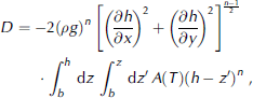
where ρ is the ice density, g is the acceleration due to gravity, h is the surface elevation and A is the temperature-dependent rate factor. To obtain Equation (4), the constitutive equation in the shallow-ice approximation is applied:


where σxz and σy z are the horizontal shear stress components. Equations (2) and (4) both contain the horizontal gradient of the surface elevation.
In this paper, the ‘CM method’ (central difference on margin) uses a centered difference scheme in the continuity equation for both the interior parts, as well as at the margin. This is in agreement with the model used by Reference Saito and Abe-OuchiSaito and Abe-Ouchi (2004). The type I or nine-point scheme (Reference Huybrechts and PayneHuybrechts and others, 1996; Reference Saito and Abe-OuchiSaito and Abe-Ouchi, 2005) is applied for computing the diffusion term D. The semi-implicit scheme (Reference Hindmarsh and PayneHindmarsh and Payne, 1996) is applied for solving the continuity equation (2).
The ‘UM method’ (upstream difference on margin) in this paper is the same as the CM method, except for an upstream finite-difference formulation at the last gridpoints before the margin. To simplify the notation, we present the corresponding numerical derivatives in one dimension (x). At interior gridpoints,


where


The surface and bedrock geometry terms, h and b, are evaluated using cubic spline interpolation at the staggered gridpoints i+½ , by assuming that the second derivative is zero at the marginal gridpoints. The horizontal gradient terms at the gridpoint i+½ are evaluated by

For the interior part, the procedure is the same for the normal type I or nine-point scheme (Reference Huybrechts and PayneHuybrechts and others, 1996; Reference Saito and Abe-OuchiSaito and Abe-Ouchi, 2005).
At the marginal gridpoints, we applied the asymmetric difference scheme. We defined the zeroth gridpoints as the last gridpoint before the margin; positive-numbered gridpoints are interior gridpoints, while negative-numbered gridpoints are zero-thickness (exterior) gridpoints.
Applying the Taylor expansion and omitting all terms with second and higher derivatives, we obtain an upstream finite-difference scheme for the derivative of q at i = 0,

The terms qand qare evaluated as shown in Equation (7).
In addition, q at i = 0, which is not at a staggered point but at a regular point, is required at the marginal gridpoint for evaluating the gradient of the flux q.
Thus, it is not necessary to evaluate q at the negative-numbered gridpoints. The surface gradients in Equation (3) are evaluated using an asymmetric second-order difference scheme, with terms at the gridpoints numbered 0, 1 and 2:

The diffusion term D 0 is also computed on the regular grid:

where

Again, D 0 includes the surface gradient terms, which are computed based on Equation (13). If the gridpoint is also a last gridpoint before the margin in the y direction, then the y gradient terms are also computed using the asymmetric scheme. In this case, interpolation is not required for evaluating the terms at i = 0. The surface gradient at the marginal gridpoints is evaluated using the same asymmetric second-order difference scheme as given in Equation (13). In this formulation, a total of nine gridpoints is used to compute the thickness evolution at either one marginal gridpoint or one interior gridpoint.
The numerical expressions for the horizontal flux gradients q in the two-dimensional form at the interior and marginal gridpoints become


All of the equations only require information from gridpoints with strictly positive ice thickness. No information from gridpoints with zero thickness is required.
Horizontal gradients of the term q in the y direction are derived correspondingly. Using the semi-implicit scheme (Reference Hindmarsh and PayneHindmarsh and Payne, 1996), the evolution of the thickness at all gridpoints (Equation (2)) requires the solution of a linear system of equations,

For the other margin and corner points, Equation (18) is modified as necessary. It should be noted that the terms Cm are coefficients computed using Equations (16) and (17). A conjugate gradient method in combination with a sparse-matrix storage scheme is applied for solving the system of linear equations, Equations (18). In principle, the upstream method can be used throughout the ice sheet, but the convergence of the conjugate gradient method may be slow. We applied the upstream method to only the last gridpoints before the margin.
The temperature distribution is calculated using the thermodynamic equation with the prescribed surface temperatures and geothermal heat flux as boundary conditions,

where k I = 2.1 Wm–1 K–1 and c p = 2009 J kg–1 K–1 are the thermal conductivity and specific heat capacity of ice, Ф is strain heating and L is a phase change term. The main difference in the numerical scheme between the present paper and Reference Saito, Abe-Ouchi and BlatterSaito and others (2006) is the difference in computing the temperature advection term. In this paper, the model uses a second-order upstream difference scheme to compute the temperature advection term, while in Reference Saito, Abe-Ouchi and BlatterSaito and others (2006) a first-order upstream scheme was used. This difference significantly influences the results, especially the temperature distribution, which is explained in section 4.2.
3. Experimental Design
An overview of all six experiments performed in this paper is shown in Table 1. All experiments were performed using the same boundary conditions as in experiment A of the EISMINT model intercomparison experiments (Reference PaynePayne and others, 2000). The bedrock topography is flat (b = 0 on all gridpoints) and kept constant throughout the time domain. The boundary conditions at the base of the ice sheet include the no-slip condition and matching geothermal heat flux. The computed temperature is constrained such that it does not exceed the local pressure-melting temperature. The surface temperature T s and surface mass balance M are functions of the horizontal distance R from the center:
List of the experiments in this paper. The two margin schemes, UM and CM, are explained in the text


where T min is the surface temperature at the center, S T is the radial surface temperature gradient, M max is the upper limit for the accumulation rate, S b is the radial mass-balance gradient and R el is the radial distance of the equilibrium line from the center. The parameters in Equations (20) and (21) are set to S b = 10–2ma–1 km–1, R el = 450 km, M max = 0.5 ma–1, S T = 1.67×10⁻²Kkm–1, T min = 238.15 K. The geothermal heat flux is uniform at 42 mWm–2 in all of the model experiments.
In all of the experiments, the grid resolution is 25 km in both horizontal coordinate directions. The vertical grid is divided into 26 levels. The time-step is 2 years for the surface evolution and the velocity field, and 10 years for the temperature field. The models are executed for 200 000 model years to reach steady state.
The first letter of an experiment name indicates the numerical scheme that was used. Experiments UU, UA and UA1 were executed using the model with the new margin scheme (UM method), and experiments CU, CA and CA1 used the old margin scheme (CM method).
The second letter of an experiment name indicates the experimental configuration. Experiments UU and CU are thermomechanically uncoupled experiments, in which the rate factors are kept constant at A = 1.0×10⁻¹⁶ma–1. These experiments are the same as the ‘moving-margin’ experiment presented in Reference Huybrechts and PayneHuybrechts and others (1996), except for a doubled horizontal resolution.
Experiments UA and CA are thermomechanically coupled experiments. The dependence of ice rheology on the computed ice temperature for these experiments is given by

where T 0 = T – T m(p)+T0 is the absolute temperature corrected for the dependence of the melting temperature T m(p) on pressure p, and T 0 = 273.15 K is the triple-point temperature of water. The values for the coefficients a and Q were taken from Reference HuybrechtsHuybrechts (1992), as follows:


These experiments apply the same configuration as in experiment A of the EISMINT model intercomparison experiments (Reference PaynePayne and others, 2000).
Experiments UA1 and CA1 are the same thermomechanically coupled experiments as UA and CA, except that they use a first-order upstream scheme for computing the temperature advection term. These experiments were used to demonstrate the difference between the methods presented in this paper and in Reference Saito, Abe-Ouchi and BlatterSaito and others (2006).
According to Reference Huybrechts and PayneHuybrechts and others (1996), the analytical margin position of the steady-state topography for all of the experiments in their paper is R = 579.81 km, which is obtained analytically by integrating Equation (1).
4. Results
4.1. Thermomechanically uncoupled model
Figure 1 shows the steady-state results for experiments UU and CU, which omit the effects of thermomechanical coupling. The simulated thicknesses are almost the same for experiments CU and UU except near the margin. Figure 1 shows the simulated thicknesses obtained by UM and CM methods near the margin. The result of CU shows splitting solutions around a distance of 570 km. In some directions, measured azimuthally from the center, the thickness is as much as 800 m, while in other directions the thickness is zero. This divergence does not occur in the results obtained from UU. The margin in UU is smoother than in CU. Thus, the improved UM method maintains the circular symmetry better than the CM method. The reason for the asymmetry in the ice-thickness distribution at the margin using the CM method is that it depends on the numerically computed surface gradient at the last gridpoint before the margin. However, the variability at the surface depends on the azimuthal direction from the center, since a quadratic grid system was used.
Steady-state solution for surface elevation, basal temperature (below pressure-melting point), vertical surface velocity component and flux divergence of all gridpoints as a function of distance from the center of the ice sheet, for experiments UU (left) and CU (right). The solid lines in (a) and (b) correspond to the analytical solution of the steady-state surface elevation. (c–h) contain only non-zero thickness gridpoints. The range of the vertical axis is the same at left and right, except for the vertical velocity plots (e, f).

Compared to the analytical solution, the thickness is still overestimated by as much as 300m (Fig. 2). However, compared with the CM method, the simulated thickness obtained by using the UM method is closer to the analytical solution by 300 m. On the other hand, the ice-sheet extension obtained by the UM method coincides with the analytical solution, while that obtained by the CM method is about 10km smaller.
Surface elevation as a function of distance from the center of the ice sheet, for experiments UU (circle) and CU (triangle). Only the marginal area is shown. The solid line corresponds to the analytical solution of the steady-state surface elevation. The dashed line corresponds to the analytical margin position (579.81 km). Note that the plots from 537 to 552 km overlap each other.

Figure 1c and d show the steady-state basal temperature distribution simulated by experiments UU and CU. The basal temperatures differ between –0.03 and 0.08 K (Fig. 3). In the region near the center, UU yields a lower temperature than CU. However, away from the center, the differences are both positive and negative.
Difference in the basal temperature (below pressure-melting point) as a function of distance from the center of the ice sheet. The result of UU minus that of CU is shown.

As shown in Reference Saito, Abe-Ouchi and BlatterSaito and others (2006), the vertical velocity component at the surface computed using CM methods shows a large scatter near the ice margin (Fig. 1f). This is because the vertical component of the velocity is related to the surface gradient, which is poorly represented near the margin in regular grids. Although some scattering is still present in the UMmethods, this feature is strongly reduced by using the improved scheme (Fig. 1e). The gap in the vertical velocity at a distance 570 km in Figure 1e is possibly caused by the change in the scheme from central to upstream.
At steady state, the flux divergence term ∇.~q in Equation (1) must equal the surface mass-balance term M. Figure 1g and h show that, in both methods, the flux divergence term agrees with Equation (21) at all model gridpoints. The simulated and analytical solutions cannot be distinguished in the figures.
4.2. Thermomechanically coupled model (EISMINT experiment)
For the thermomechanically coupled experiments, UA, CA, UA1 and CA1, no analytical solution is available except for the position of the margin. Therefore, only a comparison between UM and CM methods can be shown. First, we present the influence of the temperature advection scheme on the temperature distribution. The thermomechanically coupled experiments UA and CA are repeated with a model that uses a first-order advection scheme. These experiments are denoted by UA1 and CA1. With both the UMand CM methods using a second-order advection scheme, the ‘spoke pattern’ reported in Reference PaynePayne and others (2000) is reduced (see Fig. 4). On the other hand, the results of UA1 and CA1 show that the UM scheme does not completely eliminate the spoke pattern.
Steady-state solutions of the basal temperature (below pressure-melting point) obtained by experiments (a) UA, (b) CA, (c) UA1 and (d) CA1. (c) and (d) correspond to the results from a model with a first-order advection scheme. Shaded area indicates that the base is at the pressure-melting point. The contour interval is 2 K. Due to symmetry, only one-quarter of the sheet is shown.

Thus, despite Reference Saito, Abe-Ouchi and BlatterSaito and others (2006), the ill-conditioning of the numerical calculation of the velocity field near the margin due to the error in computing the surface gradient is not the only cause for the observed spokes in the basal temperature distribution. Experiment F of Reference PaynePayne and others (2000) with colder surface temperatures at T min = 223.15 K is repeated using both the UM and CM methods. The results show that spokes similar to those observed by Reference PaynePayne and others (2000) can be seen in both the UM and CM methods, as well as with a second-order advection scheme. At present, the reason for the poor performance of experiment F compared to experiment A is unknown. One possibility, suggested by Reference PaynePayne and others (2000), is that the spatial location of the boundary separating the cold basal ice from that at the melting point lies closer to the steep surface slopes of the ice-sheet margin, where the effects of feedback between temperature and flow are important due to the large strain heating.
However, the reduction in the spoke patterns for both the UM and CM methods in experiment A shows that the new scheme is better at determining the topography and temperature field.
Figure 5 shows the steady states simulated by experiments UA and CA using a second-order scheme to compute the temperature advection term. The irregularities in the ice thickness at the margin (Fig. 5b, at 520 km) are enhanced compared with that shown in Figure 1b.
Surface elevation, basal temperature (below pressure-melting point), vertical surface velocity component, and the flux divergence as a function of distance from the center of the ice sheet, for experiments UA (left) and CA (right). The range of the vertical axis is the same at left and right, except for the vertical velocity plots (e, f).

Figure 6 shows the simulated topography obtained by the UM and CM methods near the margin. There is a discrepancy of up to 1200m around the distance of 570 km, which stems from the result of CA. The margin in experiment UA is smoother than that of CA, which is similar to the results obtained in section 4.1 for the uncoupled experiments. The simulated thickness is corrected by as much as 600m in the marginal zone in the UA experiment. Thus, using the UM method, the computed topography near the margin becomes realistically smooth. The differences in simulated thicknesses between experiments UA and CA became smaller closer to the center of the ice sheet: 200 m at 500 m, 100m at 350 km, and 40m at the center. In addition, the improved UM method maintains the circular symmetry better than the CM method. The simulated thickness obtained for experiment UA at the analytical position of the ice margin is about 400 m. Therefore, the remaining error in the thickness is thought to be 400m at most. However, the error in the simulated thickness obtained using the UM method is expected to be reduced significantly as compared to that using the CM method.
Surface elevation as a function of distance from the center of the ice sheet, for experiments UA (circles) and CA (triangles). Only the marginal area is shown. The dashed line corresponds to the analytical margin position (579.81 km).

Figure 5c shows the steady-state basal temperature distribution simulated by experiment UA, which shows more scattering compared to the results from experiment CA (Fig. 5d). Figure 7 shows the difference in basal temperature, which is at most 0.6 K, but this is more than in the thermomechanically uncoupled case. While there is scattering in the interior part, the extent of the basal melting region is not affected. In the region near the center, UA shows lower temperatures than CA, while away from the center, UA shows both higher and lower temperature than CA.
Differences in the basal temperature (below pressure-melting point) as a function of the distance from the center of the ice sheet. The result of UA minus that of CA is shown.

As discussed in Reference Saito, Abe-Ouchi and BlatterSaito and others (2006), the vertical velocity component at the surface computed by the CM method shows a large scatter near the ice margin, which is reflected in the error of the computed surface gradient. This error in the velocity affects the temperature distribution near the margin, which in turn affects the velocity and mass flux, creating an error propagation feedback loop. Thus, the scattering in the thickness distribution may be enhanced by the thermomechanical coupling. Since the basal temperature distribution does not show the spoke pattern in experiment CA, it seems that this error in thickness is not propagated into the interior part in this experiment. In these cases, as in experiments UU and CU, the flux divergence  shows good agreement with the prescribed surface mass-balance term M at all the model gridpoints.
The difference in thickness in the coupled case is larger than in the uncoupled case, which can be explained as follows. The shear stress σxz , the shear strain rate ɛxz and the strain heating Ф can be expressed in the shallow-ice approximation by

Thickness gradient ∂H/∂x can decrease while thickness H increases. The net effect of changes in H and ∂H/∂x on the shear stress σxz depends on the topography. Figure 8 shows a comparison between the results of the two methods UA and CA at the gridpoint (525 km, 0 km). In this case, an increase in ∂H/∂x dominates, such that bottom shear stress is larger in UA than in CA at the deep part, though the thickness is smaller. Larger shear stress at the deep part results in larger strain heating. Through the temperature-dependent rate factor (Equation (22)), the corresponding horizontal velocity increases as shown in Figure8, and thus the thickness decreases.
Vertical profiles of horizontal velocity, vertical velocity, shear stress, strain heating and temperature obtained by experiments UA (circles) and CA (triangles). The values at the gridpoint (525km, 0 km) are shown.

The vertical velocity component also becomes smaller in experiment UA. At steady state, the surface boundary condition for the vertical velocity component is

Since the horizontal velocity increases, and the surface becomes steeper, w s becomes smaller in experiment UA. Due to the decrease in the vertical velocity, heat advection from the deeper part towards the surface is also decreased. However, this lowers the temperature only in the upper part. Consequently, thermomechanical coupling positively feeds back on the decrease in ice thickness. Thus, the CM method significantly overestimates the thickness near the margin in the case of thermomechanical feedback.
5. Conclusions and Prospects
In this paper, an upstream finite-difference scheme that solves the continuity equation at the margin is presented. This method improves the representation of the margin, compared to a method that uses a centered finite-difference scheme. This new method was applied to an idealized ice-sheet configuration. Comparisons were made between the upstream and central difference methods, focusing on the steady-state topography and temperature distribution. The results show that a smoother margin topography and a realistic ice thickness near the margin can be obtained by using the upstream scheme, though simulated ice thickness is still overestimated as compared to the analytical solution. In the UM method, the thickness of the interior part is only corrected by a few tens of meters, while the difference between the simulated and analytical solutions reaches a few hundred meters near the margin, due to thermomech-anical feedback. The temperature distribution is not affected significantly. Since these errors are reduced in the marginal region in the UM method, we recommend that the upstream difference scheme be used. The results indicate that the errors in the computed velocity field near the margin, which resulted from errors in the computed surface gradient, did not contribute to breaking the radial symmetry of the basal temperature distribution as was originally suspected in Reference Saito, Abe-Ouchi and BlatterSaito and others (2006). Based on the EISMINT configuration, the temperature distribution in the interior part is not affected by using the improved scheme.
The remaining errors in thickness near the margin in solving the continuity equation may be reduced by using a higher-order difference scheme. Reference Le Meur and HindmarshLe Meur and Hindmarsh (2001) explain that the accuracy is substantially increased by using a fifth-order formula. They applied their scheme to a two-dimensional ice-sheet model. Although in a three-dimensional model the procedure for building the matrix equation will be more complex and the convergence will be much slower, it is nevertheless desirable to increase the order of the scheme.
It is beyond the scope of this paper to repeat the experiments with different schemes. Implementation of a similar method on the 13-point scheme can be done by replacing all the D terms at the staggered points in Equations (16) and (17) with the average of those at the regular grids. We expect that a similar improvement (e.g. in a realistically smooth thickness distribution near the margin) could be obtained with the 13-point scheme configuration.
The surface mass-balance forcing used in this paper is a function of position only and independent of the surface elevation, since we focused on thermomechanical coupling. For realistic ice sheets, the surface mass balance and melting are most likely dependent on surface elevation. Through such elevation–melting feedback, the difference in the simulated thickness distribution between the old and the improved model is expected to increase. Thus, an ice sheet simulated by the improved model is expected to be more sensitive to changes in climate forcing than one simulated with the old model. Using a thermomechanically uncoupled ice-sheet model, Van den Berg and others (2006) showed that the effect of an inaccurate gradient in those cases would be much larger. It is expected that thermomechanical coupling would further enhance this feedback.
The focus in this paper is on steady-state solutions. Transient behavior, such as margin advancing or retreating, will need to be investigated. The response time may be affected by the chosen scheme, as presented by Van den Berg and others (2006). The test suite presented in Reference Bueler, Lingle, Kallen-Brown, Covey and BowmanBueler and others (2005) for isothermal ice sheets would be useful to determine the effects of a chosen scheme on the response time. In addition, the numerical scheme in this paper can be applied for the transformed version of the ice-sheet equation in Reference Bueler, Lingle, Kallen-Brown, Covey and BowmanBueler and others (2005), which will further decrease the errors near the ice margin.
Acknowledgements
The authors thank C. Schoof for providing useful information in the review of Reference Saito, Abe-Ouchi and BlatterSaito and others (2006). We greatly appreciate the valuable suggestions of two anonymous referees and the scientific editor T. Payne, which helped to improve the manuscript substantially. We also thank E. Bueler for adding valuable comments. This work was supported by MEXT KAKENHI 17740301.



