2.1. Base flow and stability analysis

Consider a steady fluid flow satisfying the stationary incompressible Navier–Stokes (NS) equations

(2.1)$$\begin{gather} \boldsymbol{U} \boldsymbol{\cdot} \boldsymbol{\nabla}\boldsymbol{U} + \boldsymbol{\nabla} P - \textit{Re}^{{-}1} \nabla^2 \boldsymbol{U} = \mathbf{0}, \end{gather}$$

(2.2)$$\begin{gather}\boldsymbol{\nabla} \boldsymbol{\cdot} \boldsymbol{U} = 0, \end{gather}$$

where $P(\boldsymbol {x})$ is the pressure field and $\boldsymbol {U}(\boldsymbol {x})=(U,V)^\textrm {T}$ or $(U,V,W)^\textrm {T}$ is the velocity vector in two or three dimensions. Equations are made dimensionless with a characteristic velocity $U_\infty$, a characteristic length scale $D$ and the fluid kinematic viscosity $\nu$, thus defining the Reynolds number $\textit {Re}=U_\infty D /\nu$. In the following, all velocity fields are incompressible and the continuity equation is omitted.

The linear stability of the base flow is determined by the temporal evolution of small perturbations $\boldsymbol {u}'$. Considering, in particular, the normal mode ansatz $\boldsymbol {u}'(\boldsymbol {x},t) = \boldsymbol {u}(\boldsymbol {x}) \textrm {e}^{\lambda t} + \textrm {c.c.}$, the (complex) eigenmodes $\boldsymbol {u}(\boldsymbol {x})$ are solutions of the linearised NS equations

(2.3)\begin{equation} \lambda\boldsymbol{u} + \boldsymbol{U} \boldsymbol{\cdot} \boldsymbol{\nabla}\boldsymbol{u} + \boldsymbol{u} \boldsymbol{\cdot} \boldsymbol{\nabla}\boldsymbol{U} + \boldsymbol{\nabla} p - \textit{Re}^{{-}1} \nabla^2 \boldsymbol{u} = \mathbf{0}. \end{equation}

The real and imaginary parts of an eigenvalue $\lambda$ represent the linear growth rate $\lambda _r$ and linear frequency $\lambda _i$ of the associated eigenmode. The base flow is linearly unstable if at least one mode has a positive growth rate. In compact form, (2.1)–(2.2) for the steady base flow and (2.3) for the eigenmodes can be expressed as

(2.4)$$\begin{gather} \boldsymbol{N}(\boldsymbol{U}) = \mathbf{0}, \end{gather}$$

(2.5)$$\begin{gather}(\lambda \boldsymbol{I} +\boldsymbol{A}) \boldsymbol{u} = \mathbf{0}. \end{gather}$$

Here $\boldsymbol {N}$ and $\boldsymbol {A}$ are the nonlinear and linearised Navier–Stokes operators, and $\boldsymbol {I}$ is the identity operator:

(2.6)$$\begin{gather} \boldsymbol{N}(\boldsymbol{U}) =\boldsymbol{U} \boldsymbol{\cdot} \boldsymbol{\nabla}\boldsymbol{U} + \boldsymbol{\nabla} P - \textit{Re}^{{-}1} \nabla^2 \boldsymbol{U}, \end{gather}$$

(2.7)$$\begin{gather}\boldsymbol{A}(\boldsymbol{U}) \boldsymbol{u} =\boldsymbol{U} \boldsymbol{\cdot}\boldsymbol{\nabla}\boldsymbol{u} + \boldsymbol{u}\boldsymbol{\cdot} \boldsymbol{\nabla}\boldsymbol{U} +\boldsymbol{\nabla} p - \textit{Re}^{{-}1} \nabla^2\boldsymbol{u} . \end{gather}$$

2.2. Eigenvalue sensitivity to small-amplitude steady control

Assume now that a small-amplitude control is applied via a body force acting on the steady base flow:

(2.8)\begin{equation} \boldsymbol{N}(\boldsymbol{U}) = \epsilon \boldsymbol{F}, \end{equation}

where $\|\boldsymbol {F}\|=1$ and $0< \epsilon \ll 1$. This control modifies the base flow, eigenmodes and eigenvalues, which can be expressed as power series expansions (Hinch Reference Hinch1991):

(2.9)$$\begin{gather} \boldsymbol{U} = \boldsymbol{U}_0+\epsilon\boldsymbol{U}_1+\epsilon^2\boldsymbol{U}_2+\cdots, \end{gather}$$

(2.10)$$\begin{gather}\boldsymbol{u} = \boldsymbol{u}_0+\epsilon\boldsymbol{u}_1+\epsilon^2\boldsymbol{u}_2+\cdots, \end{gather}$$

(2.11)$$\begin{gather}\lambda = \lambda_0 +\epsilon \lambda_1 +\epsilon^2 \lambda_2 +\cdots. \end{gather}$$

Injecting the expansion (2.9) into the base flow equation (2.8) yields the following at orders $\epsilon ^0$, $\epsilon ^1$ and $\epsilon ^2$:

(2.12)$$\begin{gather} \boldsymbol{N}(\boldsymbol{U}_0) = \mathbf{0}, \end{gather}$$

(2.13)$$\begin{gather}\boldsymbol{A}_0 \boldsymbol{U}_1 = \boldsymbol{F}, \end{gather}$$

(2.14)$$\begin{gather}\boldsymbol{A}_0 \boldsymbol{U}_2 ={-} \boldsymbol{U}_1 \boldsymbol{\cdot} \boldsymbol{\nabla} \boldsymbol{U}_1, \end{gather}$$

where $\boldsymbol {A}_0=\boldsymbol {A}(\boldsymbol {U}_0)$ is the NS operator linearised about the uncontrolled base flow $\boldsymbol {U}_0$, i.e. $\boldsymbol {A}_0 \boldsymbol {U}_n = \boldsymbol {U}_0 \boldsymbol {\cdot }\boldsymbol {\nabla }\boldsymbol {U}_n + \boldsymbol {U}_n\boldsymbol {\cdot } \boldsymbol {\nabla }\boldsymbol {U}_0 +\boldsymbol {\nabla } P_n - \textit {Re}^{-1} \nabla ^2 \boldsymbol {U}_n$ for $n=1,2$. Although the focus of this study is on first and second orders, note that the steady force $\boldsymbol {F}$ modifies the base flow at higher orders too, due to the nonlinear term of the NS operator.

Similarly, injecting the expansions (2.9)–(2.11) into the eigenvalue problem (2.5) yields the following at orders $\epsilon ^0$, $\epsilon ^1$ and $\epsilon ^2$:

(2.15)$$\begin{gather} (\lambda_0 \boldsymbol{I}+\boldsymbol{A}_0) \boldsymbol{u}_0 = \mathbf{0}, \end{gather}$$

(2.16)$$\begin{gather}(\lambda_0 \boldsymbol{I}+\boldsymbol{A}_0) \boldsymbol{u}_1 ={-}(\lambda_1\boldsymbol{I}+\boldsymbol{A}_1) \boldsymbol{u}_0, \end{gather}$$

(2.17)$$\begin{gather}(\lambda_0\boldsymbol{I}+\boldsymbol{A}_0) \boldsymbol{u}_2 ={-}(\lambda_1\boldsymbol{I}+\boldsymbol{A}_1) \boldsymbol{u}_1-(\lambda_2\boldsymbol{I}+\boldsymbol{A}_2) \boldsymbol{u}_0, \end{gather}$$

where the operators $\boldsymbol {A}_1$ and $\boldsymbol {A}_2$ are linear in $\boldsymbol {U}_1$ and $\boldsymbol {U}_2$, respectively, and do not depend on any other field,

(2.18a,b)\begin{equation} \boldsymbol{A}_1 = \boldsymbol{U}_1 \boldsymbol{\cdot} \boldsymbol{\nabla}({\ast})+ (\ast) \boldsymbol{\cdot} \boldsymbol{\nabla} \boldsymbol{U}_1,\quad \boldsymbol{A}_2 =\boldsymbol{U}_2 \boldsymbol{\cdot} \boldsymbol{\nabla}({\ast}) + (\ast)\boldsymbol{\cdot} \boldsymbol{\nabla} \boldsymbol{U}_2. \end{equation}

Before moving on to determining the first- and second-order eigenvalue variations $\lambda _1$ and $\lambda _2$, note that the operator $\lambda _0\boldsymbol {I} + \boldsymbol {A}_0$ is singular, since (2.15) holds. Therefore, according to the Fredholm alternative, commonly used in the context of weakly nonlinear expansions (see e.g. Sipp & Lebedev Reference Sipp and Lebedev2007), (2.16)–(2.17) can be solved for $\boldsymbol {u}_1$ and $\boldsymbol {u}_2$ if and only if their right-hand sides have no component in the direction of the eigenmode $\boldsymbol {u}_0$, i.e. no projection on the adjoint mode $\boldsymbol {u}_0^{\dagger}$. Recall that the adjoint mode is a solution of

(2.19)\begin{equation} ( \bar{\lambda}_0\boldsymbol{I} + \boldsymbol{A}_0^{\dagger} ) \boldsymbol{u}_0^{\dagger} = \mathbf{0}, \end{equation}

where the overbar stands for complex conjugation, and $\boldsymbol {A}_0^{\dagger}$ is the adjoint NS operator for the $L^2$ inner product ${({\boldsymbol {a}}\mid {\boldsymbol {b}})} = \iint \bar {\boldsymbol {a}}^\textrm {T} \boldsymbol {b} \, \mathrm {d}\kern0.06em\boldsymbol {x}$ for any $\boldsymbol {a}$, $\boldsymbol {b}$,

(2.20)\begin{equation} \boldsymbol{A}_0^{\dagger} \boldsymbol{u}_0^{\dagger}={-}\boldsymbol{U}_0\boldsymbol{\cdot}\boldsymbol{\nabla} \boldsymbol{u}_0^{\dagger} + \boldsymbol{u}_0^{\dagger} \boldsymbol{\cdot}\boldsymbol{\nabla}\boldsymbol{U}_0^\textrm{T} -\boldsymbol{\nabla} p_0^{\dagger} - \textit{Re}^{{-}1} \nabla^2 \boldsymbol{u}_0^{\dagger} , \end{equation}

such that ${({ \boldsymbol {a}}\mid { \boldsymbol {A}_0 \boldsymbol {b}})} = {({ \boldsymbol {A}_0^{\dagger} \boldsymbol {a}}\mid {\boldsymbol {b}})}$ for any $\boldsymbol {a}$, $\boldsymbol {b}$. In particular, projecting the left-hand side of (2.16)–(2.17) on $\boldsymbol {u}_0^{\dagger}$ necessarily yields zero:

(2.21)\begin{equation} {({ \boldsymbol{u}_0^{\dagger}}\mid{ ( \lambda_0\boldsymbol{I} + \boldsymbol{A}_0) \boldsymbol{u}_n})} = {({ ( \bar{\lambda}_0\boldsymbol{I} + \boldsymbol{A}_0^{\dagger} ) \boldsymbol{u}_0^{\dagger}}\mid{\boldsymbol{u}_n})} = 0, \quad n=1,2. \end{equation}

Choosing the normalisation ${({ \boldsymbol {u}_0^{\dagger} }\mid { \boldsymbol {u}_0})}=1$, the eigenvalue variations are obtained by projecting (2.16)–(2.17) on $\boldsymbol {u}_0^{\dagger}$ (Hinch Reference Hinch1991; Chomaz Reference Chomaz2005; Giannetti & Luchini Reference Giannetti and Luchini2007):

(2.22)$$\begin{gather} \lambda_1 ={-}{({ \boldsymbol{u}_0^{\dagger} }\mid{{\boldsymbol{A}}_1 \boldsymbol{u}_0})}, \end{gather}$$

(2.23)$$\begin{gather}\lambda_2 ={-}{\left({ \boldsymbol{u}_0^{\dagger} }\,{\Bigg\vert}\,{ \underbrace{\boldsymbol{A}_2\boldsymbol{u}_0}_{\text{I}} + \underbrace{(\lambda_1\boldsymbol{I}+\boldsymbol{A}_1)\boldsymbol{u}_1}_{\text{II}} }\right)}. \end{gather}$$

Any arbitrary component along $\boldsymbol {u}_0$ can be added to $\boldsymbol {u}_1$ and (2.16) will still hold, because of (2.15). This arbitrary component does not influence $\lambda _2$, because (2.16) also implies that ${({\boldsymbol {u}_0^{\dagger} }\mid {(\lambda _1 \boldsymbol {I} + \boldsymbol {A}_1)\boldsymbol {u}_0})}=0$.

The two terms in (2.23) correspond to different mechanisms: term I is the effect of the second-order base flow modification $\boldsymbol {U}_2$ (via the first-order flow modification and the nonlinear term of the NS operator); term II is the effect of the interaction between the first-order flow modification $\boldsymbol {U}_1$ and the first-order eigenmode modification $\boldsymbol {u}_1$. As will be discussed in § 4, these two terms can either compete or collaborate.

Given a steady force $\boldsymbol {F}$, one can compute the base flow modifications $\boldsymbol {U}_1$ and $\boldsymbol {U}_2$ from (2.13)–(2.14), build $\boldsymbol {A}_1$ and $\boldsymbol {A}_2$, and use expressions (2.22)–(2.23) to estimate the eigenvalue variation up to first order, $\lambda = \lambda _0 + \epsilon \lambda _1 + O(\epsilon ^2)$, and up to second order, $\lambda = \lambda _0 + \epsilon \lambda _1 + \epsilon ^2 \lambda _2 + O(\epsilon ^3)$. This involves solving linear systems only, which avoids computing the nonlinear controlled flow $\boldsymbol {U}$ and solving the eigenvalue problem for the controlled mode $\boldsymbol {u}$, thus reducing the computational cost. For instance, the dashed lines in figure 1 may be obtained by computing $\lambda _{1r}$ this way. However, the procedure must be repeated every time a different force $\boldsymbol {F}$ is considered, which may become prohibitively expensive. More useful expressions for $\lambda _1$ and $\lambda _2$ can be obtained that do not depend explicitly on $\boldsymbol {U}_1$ and $\boldsymbol {U}_2$, as explained in the next section.

2.3. Sensitivity operators

Because the operator $\boldsymbol {A}_1$ is linear in $\boldsymbol {U}_1$, which itself depends linearly on $\boldsymbol {F}$, the first-order eigenvalue variation (2.22) can be recast as

(2.24)\begin{equation} \lambda_1 = {({\boldsymbol{S}_1}\mid{\boldsymbol{F}})}, \end{equation}

where the vector field $\boldsymbol {S}_1$ is the usual sensitivity to a steady force (Marquet et al. Reference Marquet, Sipp and Jacquin2008; Meliga et al. Reference Meliga, Sipp and Chomaz2010), and depends only on the uncontrolled base flow $\boldsymbol {U}_0$ and the uncontrolled direct and adjoint modes $\boldsymbol {u}_0$ and $\boldsymbol {u}_0^{\dagger}$ (see Appendix B). This formulation offers a significant advantage: $\boldsymbol {S}_1$ can be calculated once and for all, and then used to predict the first-order effect of any steady force. Since no base flow modification $\boldsymbol {U}_1$ is ever calculated, evaluating $\lambda _1$ for a large number of steady forces becomes straightforward. For instance, figure 5(a) shows the real part of the streamwise component of $\boldsymbol {S}_1$. The value displayed at each location $\boldsymbol {x}_c$ is the first-order sensitivity of the growth rate to a steady force $\boldsymbol {F}=(\delta (\boldsymbol {x}-\boldsymbol {x}_c),0)^\textrm {T}$ localised at that point and oriented along the streamwise direction.

In a similar way, because (2.23) is quadratic in $\boldsymbol {U}_1$ and thus in $\boldsymbol {F}$, the second-order eigenvalue variation can be recast as

(2.25)\begin{equation} \lambda_2 = {({\boldsymbol{F}}\mid{\boldsymbol{S}_2 \boldsymbol{F}})}, \end{equation}

where $\boldsymbol {S}_2$ is a linear operator that, again, depends only on the uncontrolled fields $\boldsymbol {U}_0$, $\boldsymbol {u}_0$ and $\boldsymbol {u}_0^{\dagger}$. The derivation steps from (2.23) to (2.25) introduce suitable adjoint operators (see Appendix B), following the same steps as Boujo et al. (Reference Boujo, Fani and Gallaire2019) for spanwise-periodic controls in nominally spanwise-invariant flows (where $\lambda _1=0$ and the expression for $\boldsymbol {S}_2$ is slightly simpler). Again, this formulation suppresses the need to calculate the base flow modifications $\boldsymbol {U}_1$ and $\boldsymbol {U}_2$. Once $\boldsymbol {S}_2$ is available, $\lambda _2$ can be readily evaluated for any steady force. The dashed lines in figure 1 can now be obtained simply by probing $\boldsymbol {S}_1(\boldsymbol {x}_c)$ at each control location $\boldsymbol {x}_c$ of interest.

Second-order variations are obtained just as easily, and results for the few control locations considered earlier are shown as solid lines in figure 2. The predicted growth rate variation is generally improved. In figure 2(b,d), for instance, the second-order prediction follows closely the actual growth rate variation up to much larger amplitudes than the first-order prediction. In other locations, however, like in figure 2(a,c), the improvement is less significant, owing to higher-order variations. Figure 2(e–h) highlights these higher-order variations, confirming their importance (figure 2e,g) or lack thereof (figure 2f,h).

Figure 2.

Second-order sensitivity improves the prediction of growth rate variation. (a–d) Same data as figure 1, together with second-order prediction (solid line). (e–h) Higher-order variation: nonlinear data, i.e. all terms of order $n \geqslant 2$ (symbols), and second-order sensitivity (solid line).

As will be discussed in § 4, sensitivity maps can be produced that allow one to identify at a glance regions where a steady force alters the eigenvalue most effectively. Further, the relative signs and magnitudes of the first- and second-order eigenvalue variations will characterise the usefulness of the first-order sensitivity.

Before moving on to the next sections, it is worth mentioning that the method can be applied to the sensitivity of other quantities, as soon as they are defined as eigenvalue problems. To illustrate this point, Appendix C derives the first- and second-order sensitivities of the linear amplification of harmonic forcing (resolvent gain).

2.4. Higher-order sensitivity

Higher-order terms $\boldsymbol {U}_n$ for the base flow modification are governed by

(2.26)\begin{align} \boldsymbol{A}_0 \boldsymbol{U}_3 &={-} \boldsymbol{U}_1 \boldsymbol{\cdot} \boldsymbol{\nabla} \boldsymbol{U}_2 - \boldsymbol{U}_2 \boldsymbol{\cdot} \boldsymbol{\nabla} \boldsymbol{U}_1,\\ &~\vdots\nonumber\end{align}

(2.27)\begin{align} \boldsymbol{A}_0 \boldsymbol{U}_n &= \sum_{1 \leqslant m \leqslant n-1} - \boldsymbol{U}_m \boldsymbol{\cdot} \boldsymbol{\nabla} \boldsymbol{U}_{n-m}.\end{align}

Similarly, higher-order terms $\boldsymbol {u}_n$ for the eigenmode modification are governed by

(2.29)\begin{align} (\lambda_0 \boldsymbol{I}+\boldsymbol{A}_0) \boldsymbol{u}_3 &={-}(\lambda_1 \boldsymbol{I}+\boldsymbol{A}_1) \boldsymbol{u}_2 -(\lambda_2 \boldsymbol{I}+\boldsymbol{A}_2) \boldsymbol{u}_1 -(\lambda_3 \boldsymbol{I}+\boldsymbol{A}_3) \boldsymbol{u}_0, \\ &~\vdots\nonumber\end{align}

(2.30)\begin{align} (\lambda_0\boldsymbol{I}+\boldsymbol{A}_0) \boldsymbol{u}_n &= \sum_{1\leqslant m \leqslant n} -(\lambda_m \boldsymbol{I}+\boldsymbol{A}_m) \boldsymbol{u}_{n-m}, \end{align}

which, upon projection onto $\boldsymbol {u}_0^{\dagger}$, yields the eigenvalue variations (Hinch Reference Hinch1991; Mensah et al. Reference Mensah, Orchini and Moeck2020):

(2.32)\begin{align} \lambda_3 &={-}{({ \boldsymbol{u}_0^{\dagger} }\mid{ \boldsymbol{A}_3 \boldsymbol{u}_0 })} -{({ \boldsymbol{u}_0^{\dagger} }\mid{ (\lambda_1 \boldsymbol{I}+\boldsymbol{A}_1) \boldsymbol{u}_{2} + (\lambda_2 \boldsymbol{I}+\boldsymbol{A}_2) \boldsymbol{u}_{1} })},\\ &~\vdots\nonumber\end{align}

(2.33)\begin{align} \lambda_n &={-}{({ \boldsymbol{u}_0^{\dagger} }\mid{ \boldsymbol{A}_n \boldsymbol{u}_0 })} -\sum_{1\leqslant m \leqslant n-1} {({ \boldsymbol{u}_0^{\dagger} }\mid{ (\lambda_m \boldsymbol{I}+\boldsymbol{A}_m) \boldsymbol{u}_{n-m} })}. \end{align}

Just like $\lambda _1$ and $\lambda _2$ are linear and quadratic in $\boldsymbol {U}_1$, respectively, each of the above expressions is exactly proportional to $\boldsymbol {U}_1^n$, and thus to $\boldsymbol {F}^n$. In principle, one can therefore generalise expressions (2.24)–(2.25), which involve the vector $\boldsymbol {S}_1$ (tensor of order one) and the matrix $\boldsymbol {S}_2$ (tensor of order two), and introduce tensors $\boldsymbol {S}_n$ of order $n$ such that

(2.35)\begin{align} \lambda &= \lambda_0 + \epsilon \lambda_1 + \epsilon^2 \lambda_2 + \epsilon^3 \lambda_3 + \cdots + \epsilon^n \lambda_n + \cdots \nonumber\\ &= \lambda_0 + \epsilon \iint ( \boldsymbol{S}_1 )_i \boldsymbol{F}_i\,\mathrm{d}\kern0.06em \boldsymbol{x} + \epsilon^2 \iint ( \boldsymbol{S}_2 )_{ij} \boldsymbol{F}_i \boldsymbol{F}_j\,\mathrm{d}\kern0.06em \boldsymbol{x} + \epsilon^3 \iint ( \boldsymbol{S}_3 )_{ijk} \boldsymbol{F}_j \boldsymbol{F}_j\boldsymbol{F}_k \,\mathrm{d}\kern0.06em \boldsymbol{x} + \cdots \nonumber\\ &\quad + \epsilon^n \iint ( \boldsymbol{S}_n )_{i_1 i_2 \ldots i_n} \boldsymbol{F}_{i_1} \boldsymbol{F}_{i_2} \cdots \boldsymbol{F}_{i_n} \,\mathrm{d}\kern0.06em \boldsymbol{x} + \cdots, \end{align}

with Einstein notation for repeated indices. Conceptually, the method for obtaining the higher-order sensitivity operators $\boldsymbol {S}_n$ is similar to that described in Appendix B, and involves a combination of the following steps: (i) redefine linear forms like $\boldsymbol {A}_n \boldsymbol {u}_0$, $(\lambda _m \boldsymbol {I}+\boldsymbol {A}_m) \boldsymbol {u}_{n-m}$, etc., so as to make explicit the dependence on the first-order flow modification $\boldsymbol {U}_1$, and eventually on the force $\boldsymbol {F} = \boldsymbol {A}_0 \boldsymbol {U}_1$; (ii) introduce adjoint operators so as to isolate $\boldsymbol {F}$, and identify the remaining control-independent operator as the sensitivity $\boldsymbol {S}_n$.

It should be noted that adding more terms to the power series (2.11) does not necessarily improve its accuracy, and it certainly does not for amplitudes larger than the radius of convergence $r$ of the expansion. In general, $r$ depends on both the type and location of the control. In order to rigorously assess the validity of a second-order or higher-order sensitivity prediction, one must therefore compute the eigenvalue $\lambda$ of the actual nonlinear controlled flow, similar to validation calculations for first-order sensitivity prediction.

2.5. Computational cost

The cost of computing the effect of a steady force on the eigenvalue is estimated in table 1. Different methods are compared: computing the fully nonlinear controlled flow and associated eigenvalue $\lambda$; and computing the first- and second-order eigenvalue variations $\lambda _1$ and $\lambda _2$ using sensitivity operators. In what follows, $N$ is the total number of degrees of freedom after numerical discretisation, and $M$ is the number of independent forcing locations. The uncontrolled base flow $\boldsymbol {U}_0$ and leading eigenmode $\boldsymbol {u}_0$ are computed prior to considering any control.

Table 1.

Computational cost for the eigenvalue variation induced by a steady force, in a system discretised with $N$ degrees of freedom and forced at $M$ locations. The dominant contribution is derived assuming $1 \ll M \ll N$. Recomputing the controlled base flow and the corresponding eigenvalue for each forcing location is substantially more expensive than evaluating the sensitivities.

For the sake of simplicity, it is reasonable to assume that $1 \ll M \ll N$ when estimating the leading-order computational cost. That is, $M$ must be rather large so as to obtain sufficiently fine-grained sensitivity maps, and $N$ must be large enough to compute the eigenvalue and its variation accurately. To fix ideas, 10 different values for both $x_c$ and $y_c$ already yield $M=100$ control locations to be evaluated. Further, with a finite-element method, a minimum of $N=10^3$ to $10^4$ degrees of freedom seem necessary. In this study, $M \simeq 10^4$ and $N \simeq 6 \times 10^5$.

The computational cost of the different methods is as follows.

1. (a) Recomputing the fully nonlinear controlled flow and the corresponding eigenvalue $\lambda$ for each forcing location (second column of table 1) involves two steps: (i) computing $M$ nonlinear base flows $\boldsymbol {U}$, for instance with a Newton method requiring $k$ linear system resolutions (typically five to ten iterations) of complexity $O(N^3)$; (ii) solving $M$ eigenvalue problems for $\boldsymbol {u}$, for instance with an implicitly restarted Arnoldi method, of complexity proportional to $O(N^2)$. Omitting constant factors for simplicity, the total cost scales like $M \times O(N^3)$.

2. (b) Estimating the first- and second-order eigenvalue variations with (2.24)–(2.25), i.e. with sensitivity operators (third and fourth columns of table 1), involves the following steps (see details in Appendix B): (i) computing once and for all the (uncontrolled) adjoint mode $\boldsymbol {u}_0^{\dagger}$, with a cost proportional to $O(N^2)$; (ii) computing once and for all the lower–upper (LU) decompositions of complexity $O(N^3)$ of $\boldsymbol {A}_0^{\dagger}$ and $(\lambda _0\boldsymbol {I} + \boldsymbol {A}_0)$ for $\lambda _1$ and $\lambda _2$, respectively; (iii) evaluating a few matrix–vector products, with a cost $O(N^2)$ for each forcing location. The total cost therefore scales like $O(N^3)$, for both $\lambda _1$ and $\lambda _2$.

In conclusion, computing $\lambda _2$ involves an additional cost similar to that of computing $\lambda _1$. It is much smaller than that of recomputing the nonlinear eigenvalue $\lambda$ for each forcing location. The advantage of adjoint methods therefore applies to both first and second orders. Of course, this is true only when a large number $M$ of control locations are considered, e.g. when constructing sensitivity maps. Conversely, when only a few control locations are of interest, calculating the actual eigenvalue $\lambda$ is more accurate and not significantly more computationally expensive.

In the above analysis, memory requirements have not been considered. Storage is not an issue for two-dimensional configurations, and for spatial discretisation methods that yield sparse matrices (e.g. finite-element method), but may become prohibitive for three-dimensional configurations or methods that yield dense matrices (e.g. spectral methods). This is a practical limitation of the proposed approach. For standard eigenvalue calculations and first-order sensitivity analysis, one can use matrix-free time-stepping techniques as an alternative to matrix-based techniques (Tuckerman & Barkley Reference Tuckerman and Barkley2000). Whether such an approach is possible for second-order sensitivity analysis remains to be determined.

3.1. Base flow

A two-dimensional triangulation of the domain

(3.1)\begin{equation} \varOmega=\{ (x,y) \mid {-}10 \leqslant x \leqslant 50, |y| \leqslant 10, \sqrt{x^2+y^2}\geqslant 0.5 \} \end{equation}

is generated with the finite-element software FreeFem$++$ (Hecht Reference Hecht2012), resulting in approximately 136 000 elements. Velocity and pressure fields are discretised with P2 and P1 Taylor–Hood elements, respectively, yielding a total of $N \simeq 615\,000$ degrees of freedom. All discrete operators are built from their continuous expressions (see details in Appendix B) in variational form. In particular, this means that the ‘differentiate then discretise’ approach is used for adjoint operators, as opposed to the ‘discretise then differentiate’ approach.

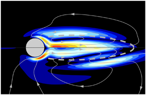
The uncontrolled steady base flow $\boldsymbol {U}=\boldsymbol {U}_0$ is obtained by solving (2.4) with a Newton method, iterated until residuals are smaller than $10^{-12}$. Boundary conditions are imposed as follows: uniform free-stream velocity at the inlet, no-slip boundary condition on the cylinder wall, outflow boundary condition $-P\boldsymbol {n} + \textit {Re}^{-1}\boldsymbol {\nabla }\boldsymbol {U}\boldsymbol {\cdot }\boldsymbol {n} =\mathbf {0}$ (with $\boldsymbol {n}$ the normal vector) at the outlet, and symmetry condition on the lateral sides of the domain. Figure 3 shows the vorticity $\omega =\omega _0=\partial _x V_0 - \partial _y U_0$ of the base flow at $\textit {Re}=50$. Shear layers of opposite vorticity are created on both sides of the cylinder. The recirculation region (dashed line) extends over three diameters downstream.

Figure 3.

Vorticity of the base flow at $\textit {Re}=50$. Dashed line: recirculation region.

Controlled base flows $\boldsymbol {U}$ are computed for validation purposes, solving (2.8) with the same method. For steady forces $\boldsymbol {F}$ that are localised in space, Dirac delta functions are smoothed out numerically into Gaussians of variance $0.0025$.

3.2. Stability analysis

The eigenvalue problem (2.5) is solved with Matlab using an implicitly restarted Arnoldi method with shift-and-invert preconditioning. This study focuses on the leading eigenmode $\boldsymbol {u}=\boldsymbol {u}_0$, which becomes unstable at $\textit {Re} \simeq 47$ via a Hopf bifurcation, as a pair of complex conjugate eigenvalues cross the imaginary axis, as illustrated in the half-plane $\lambda _i>0$ in figure 4(a) (the other half is symmetric with respect to $\lambda _i=0$). The leading eigenmode at $\textit {Re}=50$, associated with the eigenvalue $\lambda \simeq 0.0173+0.7797\textrm {i}$, is shown in figure 4(b). It is largest a few diameters downstream of the recirculation region, as perturbations are advected by the base flow. With its wave packet structure and its complex eigenvalue, this mode breaks both the spatial and temporal symmetries, leading to periodic vortex shedding and to the Bénard–von Kármán street in the cylinder wake.

Figure 4.

(a) Eigenvalues of the cylinder flow at $\textit {Re}=50$ (filled squares), and leading eigenvalue at $\textit {Re}=40$, 45, …, 100 (empty circles). The full spectrum is symmetric with respect to $\lambda _i=0$. (b) Leading eigenmode and (c) leading adjoint mode (real part, cross-stream velocity) at $\textit {Re}=50$, normalised such that ${({\boldsymbol {u}_0^{\dagger} }\mid {\boldsymbol {u}_0})}=1$ and $\|\boldsymbol {u}_0\|=1$.

The adjoint problem (2.19) is solved with the same method. The leading adjoint mode $\boldsymbol {u}_0^{\dagger}$ shown in figure 4(c) is largest in the recirculation region, and adjoint perturbations travel upstream, a consequence of upstream advection in the adjoint NS operator.

3.3. Sensitivity

First- and second-order sensitivity maps are computed for localised control forces $\boldsymbol {F}$. The control is moved within the subdomain $x \in [-2,6]$, $y \in [0,3]$, with a step size $\Delta x = \Delta y=0.05$, leading to approximately $M \simeq 10\,000$ control locations.

The second-order sensitivity operator $\boldsymbol {S}_2$ defined by (2.25) contains inverse operators (see detailed expression in Appendix B) and is therefore not formed explicitly. Instead, the LU decomposition of each operator to be inverted is precomputed once and for all, such that each subsequent matrix inversion is replaced with two simple matrix–vector products. (Note that $\boldsymbol {S}_2$ is a second-order tensor; by contrast, the first-order sensitivity $\boldsymbol {S}_1$ defined by (2.24) is a vector that can be formed explicitly and plotted without further difficulty. In this study, sensitivity maps for $\lambda _1$ and $\lambda _2$ are evaluated location by location.)

4.1. Sensitivity to a steady body force

Let us consider first a generic steady body force. Figure 5(a) shows the real part of the $x$ component of the first-order sensitivity $\boldsymbol {S}_1(\boldsymbol {x})$ to such a steady force. As shown by (2.24), the value at each location $\boldsymbol {x}=\boldsymbol {x}_c$ is also the value of the first-order variation $\lambda _{1r}$ when choosing a localised force along the $x$ direction, $\boldsymbol {F}=(\delta (\boldsymbol {x}-\boldsymbol {x}_c),0)^\textrm {T}$. The sensitivity is large and negative on the sides of the cylinder and inside the recirculation region, and positive on the sides of recirculation region, in agreement with Marquet et al. (Reference Marquet, Sipp and Jacquin2008) (figure 9(a) therein). Note that changing the sign of $F_x$ changes the sign of $\lambda _1$, such that stabilising regions ($\lambda _{1r}<0$, blue) become destabilising ($\lambda _{1r}>0$, red) and vice versa.

Figure 5.

Sensitivity of the leading mode's growth rate to a localised steady force oriented along the $x$ direction, at $\textit {Re}=50$. All fields are symmetric with respect to $y=0$. Black dots show the control locations considered in figures 1 and 2. (a) First-order variation $\lambda _{1r}$. (b) Second-order variation $\lambda _{2r}$. (c) Term I and (d) term II in the decomposition (2.23) of the second-order variation. (e) Sign of the product $\lambda _{1r} \lambda _{2r}$. (f) Relative importance of first- and second-order variations, quantified by the threshold amplitude (4.2), shown here as $\log _{10}(\epsilon _t)$. Insets: close-up views of the region $0.7 \leqslant x \leqslant 1.3$, $0.4 \leqslant y \leqslant 1.2$.

The second-order sensitivity $\boldsymbol {S}_2(\boldsymbol {x})$ is visualised in figure 5(b), which shows the second-order growth rate variation $\lambda _{2r}$ evaluated according to (2.25) for the same localised force $\boldsymbol {F}=(\delta (\boldsymbol {x}-\boldsymbol {x}_c),0)^\textrm {T}$. Overall, and in absolute value, sensitive regions are similar at first and second orders, namely, the domain approximately delimited by $0\leqslant x \leqslant 4$, $|y|\leqslant 1$, and containing the sides of the cylinder, the recirculation region and the shear layers. Note that, unlike $\boldsymbol {S}_1$, the sign of $\boldsymbol {S}_2$ does not change with the sign of $F_x$.

With these two maps available, it is now possible to explain the results of figure 2. The three control locations $\boldsymbol {x}_c=(1,0.7)$, $\boldsymbol {x}_c=(1,1)$ and $\boldsymbol {x}_c=(1,0.6)$ lie in a region of similar first-order sensitivity (figure 5a), and therefore induce similar first-order reductions $\lambda _{1r}$ (figure 2a–c). The second-order variations, however, differ substantially between these three locations (figure 5b): small in $\boldsymbol {x}_c=(1,0.7)$, negative in $\boldsymbol {x}_c=(1,1)$ and positive in $\boldsymbol {x}_c=(1,0.6)$. As a result, the second-order prediction is not much different from the first-order one in figure 2(a), and yields a larger growth rate reduction in figure 2(b) and a smaller one in figure 2(c). The second-order prediction generally follows more closely the nonlinear results than the first-order one. In the last control location, $\boldsymbol {x}_c=(3.5,0.8)$, the first-order sensitivity is small (figure 5a), yielding a weak first-order variation in figure 2(d). The second-order variation, however, is clearly negative (figure 5b), and the actual growth rate reduction is well captured by the second-order prediction (figure 2d).

Considering the large differences observed between different control locations, and the potential impact on flow restabilisation, it would be useful to find a simple way to address the following questions: (i) What is the range of control amplitude where the first-order sensitivity yields an accurate prediction? (ii) Outside this range, does it underestimate or overestimate the actual variation? One step towards answering the first question is possible with the ratio of first- to second-order variations. Recalling the expansion

(4.1)\begin{equation} \lambda = \lambda_0 + \epsilon \lambda_1 + \epsilon^2 \lambda_2 + O(\epsilon^3), \end{equation}

it appears that the second-order correction $\epsilon ^2 |\lambda _2|$ is of the same order of magnitude as the first-order variation $|\lambda - \lambda _0| = \epsilon |\lambda _1|$ for the threshold amplitude

(4.2)\begin{equation} \epsilon_t = \left| \dfrac{\lambda_1}{\lambda_2} \right|. \end{equation}

For small enough amplitudes $\epsilon \ll \epsilon _t$, the first-order variation predicts the actual variation accurately, as the second-order correction is negligible. Conversely, for large amplitudes $\epsilon \gg \epsilon _t$, the second-order variation dominates the first-order one. In between, the second-order variation becomes important and cannot be ignored when the control amplitude reaches some fraction of the threshold amplitude, say $\epsilon _t/10$.

Obviously, the analysis needs to be refined when $\lambda _2=0$. Taking into account $\epsilon ^3 \lambda _3$ or the next non-zero higher-order correction $\epsilon ^n \lambda _n$, the threshold amplitude becomes $\epsilon _t=|\lambda _1/\lambda _n|^{1/(n-1)}.$ Note that the threshold amplitude decreases as the relative importance of $\epsilon ^2 \lambda _2$ grows; this latter term becomes the leading-order term in the limiting case $\lambda _1=0$ (e.g. for the spanwise-periodic control of spanwise-invariant flows), and the threshold amplitude then becomes $\epsilon _t=|\lambda _2/\lambda _n|^{1/(n-2)}$.

Figure 5(f) shows the threshold amplitude (4.2), i.e. the ratio of the maps in figure 5($a$,$b$), in logarithmic scale. Focusing on regions where $\lambda _{1r}$ and $\lambda _{2r}$ are not both small, it appears that the first-order prediction is especially accurate up to large amplitudes ($\log _{10}(\epsilon _t)>0$, green) near the cylinder, downstream of the cylinder on the symmetry axis up to $x=2$, and in a thin strip running along and outside the recirculation region. Conversely, the second-order prediction must be taken into account ($\log _{10}(\epsilon _t)<-1$, yellow and red) in other regions both inside and outside the recirculation region, particularly in a thin strip running along and inside it. The proximity of those two strips warns about locating a steady force near the separatrix, or in any region where $\epsilon _t$ has a strong gradient: slight, unintentional shifts can dramatically increase the amplitude of the second-order variation and ruin the accuracy of the first-order prediction.

Figure 5(f) confirms observations from figure 2: $\epsilon _t$ is large and the first-order prediction is accurate over a wide range of control amplitudes in $\boldsymbol {x}_c=(1,1)$ and $\boldsymbol {x}_c=(1,0.7)$, while $\epsilon _t$ is small and the second-order variation quickly becomes important in $\boldsymbol {x}_c=(1,0.6)$ and $\boldsymbol {x}_c=(3.5,0.8)$.

The second question above is answered by considering the signs of $\lambda _{1r}$ and $\lambda _{2r}$. If both signs are identical, the second-order correction strengthens the effect of the first-order variation: when $\lambda _{1r},\lambda _{2r}<0$, the flow is stabilised even more than predicted by $\lambda _{1r}$ alone (and destabilised even more when $\lambda _{1r},\lambda _{2r}>0$), such that a smaller control amplitude is actually sufficient to obtain the desired effect. Conversely, if the signs are opposite, the effect is weakened: for example, when $\lambda _{1r}<0$ and $\lambda _{2r}>0$, the flow is not stabilised as efficiently as predicted by $\lambda _{1r}$ alone, such that a larger control amplitude is actually required to obtain the desired effect. As a way to distinguish between those two situations, figure 5$(e)$ shows the sign of the product $\lambda _{1r} \lambda _{2r}$. Focusing again on regions where $\lambda _{1r}$ and $\lambda _{2r}$ are not both small, this map indicates that ‘safe’ regions where $\lambda _{1r} \lambda _{2r}>0$ (green) are rather few and apart (mainly near the cylinder and along the separatrix), the rest being ‘dangerous’ regions where $\lambda _{1r} \lambda _{2r}<0$ (red).

Consider again the four control configurations of figure 2, where $F_x<0$ (recall that the sign of $\lambda _{1r}$ changes when the sign of $F_x$ is changed, which swaps the ‘safe’ and ‘dangerous’ regions). Figure 5(e) confirms that the first-order prediction underestimates the growth rate reduction (compared to first- and second-order predictions together) in $\boldsymbol {x}_c=(1,1)$, $\boldsymbol {x}_c=(1,0.7)$ and $\boldsymbol {x}_c=(3.5,0.8)$, and overestimates it in $\boldsymbol {x}_c=(1,0.6)$.

Let us come back to figure 5(c,d), which shows the two terms I and II in the second-order sensitivity equation (2.23), i.e. the effects of $\boldsymbol {U}_2$ and of the $\boldsymbol {U}_1$–$\boldsymbol {u}_1$ interaction, respectively. The map in figure 5(b) is the sum of those two maps, and all three colour scales are identical. Overall, terms I and II are of the same order of magnitude. Both terms display regions of positive and negative sensitivity. They collaborate to yield positive sensitivity near the downstream end of the recirculation region, and negative sensitivity on the side of the recirculation region. Conversely, they compete on part of the symmetry axis inside the recirculation region, and on part of the separatrix, resulting in a weak total sensitivity. Although the map of term I bears an overall qualitative similarity to the map of total sensitivity, term II makes a significant contribution everywhere; in other words, the steady control force modifies the growth rate at second order by changing not only the base flow but also the eigenmode that develops on that base flow.

4.2. Sensitivity to a small control cylinder

The sensitivity analysis is now applied to a practical flow control strategy, namely inserting a small passive device in order to reduce the growth rate of the leading mode. Following Hill (Reference Hill1992), and later Marquet et al. (Reference Marquet, Sipp and Jacquin2008) and Meliga et al. (Reference Meliga, Sipp and Chomaz2010), the effect of a small circular cylinder of diameter $d$ located in $\boldsymbol {x}_c$ is modelled as a steady force acting on the base flow, equal and opposite to the drag force that would be felt by that cylinder in a uniform flow with the local velocity

(4.3)\begin{equation} \epsilon \boldsymbol{F}(\boldsymbol{x}) ={-} \tfrac{1}{2} d C_d(\boldsymbol{x}) \|\boldsymbol{U}_0(\boldsymbol{x})\| \boldsymbol{U}_0(\boldsymbol{x}) \delta(\boldsymbol{x}-\boldsymbol{x}_c). \end{equation}

The drag coefficient $C_d$ of the control cylinder depends on the local Reynolds number $\textit {Re}_d = \|\boldsymbol {U}_0(\boldsymbol {x})\| d/\nu$ and is modelled here with the power law $C_d(\textit {Re}_d) = 0.8558 + 10.05 \textit {Re}_d^{-0.7004}$ (Boujo & Gallaire Reference Boujo and Gallaire2014; Meliga et al. Reference Meliga, Boujo, Pujals and Gallaire2014) meant to approximate data from the literature (Finn Reference Finn1953; Tritton Reference Tritton1959) and in-house numerical simulations in the range of interest $1 \lesssim \textit {Re}_d \lesssim 15$. In the following, results are illustrated with $d=0.1$, i.e. a control cylinder 10 times smaller than the main cylinder.

The first-order growth rate variation induced by the control cylinder is displayed in figure 6(a). The map shows a destabilising region on the sides of the main cylinder, stabilising regions on the sides of the recirculation region, and more weakly stabilising regions on the symmetry axis both upstream and downstream of the main cylinder. This is in agreement with the map obtained by Marquet et al. (Reference Marquet, Sipp and Jacquin2008) (figure 11(a) therein), and is consistent with the map of figure 5(a), since the force (4.3) is oriented mainly along $-x$ outside the recirculation region and mainly along $x$ inside.

Figure 6.

Growth rate variation induced by a small control cylinder of diameter $d=0.1$ at $\textit {Re}=50$: (a) $\epsilon \lambda _{1r}$ and (b) $\epsilon ^2 \lambda _{2r}$. (c) Term I and (d) term II in the decomposition of $\epsilon ^2 \lambda _{2r}$. (e) Sign of the product $\lambda _{1r} \lambda _{2r}$. (Figure 5(f) has no equivalent here because the diameter $d$, and therefore the amplitude $\epsilon$, are fixed.) The black dot shows the location $\boldsymbol {x}_c=(1,1)$ investigated in § 4.3.

Figure 6(b) shows the second-order growth rate variation. The main destabilising and stabilising regions appear rather similar to those of the first-order variation of figure 6(a). This means that, where the signs of those regions do correspond, the second-order variation tends to strengthen the effect of the first-order one. A closer look at figure 6(e) reveals that, where $\lambda _{1r}$ and $\lambda _{2r}$ are not both small, they generally have the same sign. Therefore, for a small control cylinder, and considering the variation of $\lambda _r$ up to second order, the situation is one of the following almost everywhere: (i) both $\lambda _{1r}$ and $\lambda _{2r}$ are small, so the control cylinder does not modify the growth rate substantially; (ii) only $\lambda _{2r}$ is small, so the effect of the control cylinder is well predicted by $\lambda _{1r}$ alone; (iii) $\lambda _{1r}$ and $\lambda _{2r}$ are not small and have the same sign, so the effect of the control cylinder is stronger (more destabilising or more stabilising) than predicted by $\lambda _{1r}$ alone. One exception is the narrow region where $\lambda _{2r}>0$ and $\lambda _{1r}$ is small: although first-order sensitivity predicts no effect, the control cylinder is actually destabilising.

The decomposition of $\lambda _{2r}$ into terms I and II in figure 6(c,d) shows that the second-order destabilising effect is primarily due to $\boldsymbol {U}_2$, while the second-order stabilising effect is due both to $\boldsymbol {U}_2$ and to the $\boldsymbol {U}_1$–$\boldsymbol {u}_1$ interaction.

Figure 7(a,b) shows the contours where inserting a small control cylinder of diameter $d=0.1$, as described above, is predicted to make the leading mode neutrally stable. Several Reynolds numbers $\textit {Re} \geqslant 50$ are considered. Inside the regions delimited by these contours, the mode is stable and vortex shedding is expected to be suppressed. In figure 7(a), only the first-order sensitivity prediction is considered, $\lambda _{0r} + \epsilon \lambda _{1r}=0$, while in figure 7(b), the second-order correction is included too, $\lambda _{0r} + \epsilon \lambda _{1r} + \epsilon ^2\lambda _{2r}=0$. The results compare qualitatively well with the experimental observations of Strykowski & Sreenivasan (Reference Strykowski and Sreenivasan1990) (figure 20 therein): stabilisation is achieved on the side of the recirculation region, in an area that is rather wide at $\textit {Re}=50$ and that becomes smaller as the Reynolds number increases, until shrinking to a single point and vanishing when restabilisation is not possible any more. Compared to the first-order sensitivity, however, the second-order sensitivity seems to better capture the results of Strykowski & Sreenivasan (Reference Strykowski and Sreenivasan1990): in particular, it predicts a wider stabilising area at $\textit {Re}=60$, and a larger value of the maximum stabilisable Reynolds number $70<\textit {Re}<80$.

Figure 7.

Passive control with (a,b) one cylinder or (c,d) two symmetric cylinders modelled by the force (4.3) for a diameter $d=0.1$. On the contours, sensitivity analysis predicts the leading mode to be stabilised, i.e. become exactly neutrally stable. (a,c) First-order prediction, $\lambda _{0r} + \epsilon \lambda _{1r} = 0$; (b,d) second-order prediction, $\lambda _{0r} + \epsilon \lambda _{1r} + \epsilon ^2 \lambda _{2r} = 0$. Reynolds numbers $\textit {Re}=50, 60, \ldots , 100$. Contours are symmetric with respect to $y=0$.

For completeness, figure 7(c,d) shows stabilising contours for a pair of control cylinders located symmetrically in $(x_c,y_c)$ and $(x_c,-y_c)$, still with $d=0.1$. In the sensitivity framework, the two cylinders are assumed not to influence each other, which is not satisfied close to the symmetry axis $y=0$. Unsurprisingly, the main stabilising region is wider but still located on the side of the recirculation region. Although conclusions should be drawn with care at larger Reynolds numbers, as the uncontrolled flow becomes linearly unstable to a second two-dimensional mode at $\textit {Re}\simeq 100$ (Verma & Mittal Reference Verma and Mittal2011) and to a three-dimensional mode at $\textit {Re} \simeq 190$ (Barkley & Henderson Reference Barkley and Henderson1996), restabilisation can be achieved up to $\textit {Re}\simeq 100$ and $\textit {Re} > 100$ according to first- and second-order sensitivity predictions, respectively.

4.3. Analysis of the stabilisation induced by a small control cylinder located optimally

In this section, the effect of a small control cylinder is investigated in more detail for the specific control location $\boldsymbol {x}_c=(1,1)$, close to the location of largest first- and second-order stabilising effects identified in § 4.2.

Figure 8 shows the eigenspectrum of the flow controlled with a secondary cylinder of increasing diameter $d$. The leading mode is restabilised for diameters $d \gtrsim 0.004$. Other modes remain stable for the whole range of diameters investigated. As seen in the close-up (figure 8b), the second-order sensitivity (thick solid line) follows closely the actual path of the leading eigenvalue in the complex plane (symbols), accurately capturing both the growth rate and the frequency, and improving on the first-order prediction (dashed line).

Figure 8.

(a) Eigenvalues of the uncontrolled flow (black squares), and of the flow controlled with a small secondary cylinder of diameter $d$ (triangles, $d=0.03$; circles, $d=0.05$; diamonds, $d=0.1$) located in $\boldsymbol {x}_c=(1,1)$. (b) Zoomed-in view of the leading eigenvalue (dashed region in panel (a)), with first- and second-order sensitivities (dashed and solid lines, respectively). $\textit {Re}=50$.

Let us now focus on the diameter $d=0.1$. As apparent from figure 6, the predicted first- and second-order growth rate variations are comparable,

(4.4a,b)\begin{equation} \epsilon\lambda_{1r} ={-}0.0426, \quad \epsilon^2\lambda_{2r} ={-}0.0424, \end{equation}

and the two second-order contributions are of similar order of magnitude: $\epsilon ^2\lambda _{2r,\text {I}} = -0.0258$, $\epsilon ^2\lambda _{2r,\text {II}} = -0.0167$. Figure 9 depicts the base flow modification. At first order, the control cylinder induces a strong velocity deficit $U_1<0$ in its wake, and a slight acceleration $U_1>0$ between the two cylinders (figure 9a). As a result, two layers of opposite vorticity emanate from the control cylinder (figure 9b) in a roughly symmetric way. At second order, velocity and vorticity are modified more weakly, with a more complicated spatial pattern (figure 9c,d). The net effect of the control cylinder is best illustrated by the velocity and shear profiles in figure 9(e). In $x=0.8$, just upstream of the control location $x_c=1$, the flow modification $U_1$ (red dashed line) smooths the velocity profile and reduces the maximum shear. Downstream ($x=1.5$ and 2), the induced velocity deficit further reduces shear in the lower shear layer emanating from the control cylinder, where the positive vorticity $\omega _1$ (figure 9b) counteracts the negative base flow vorticity $\omega _0$ (figure 3). These observations are consistent with those of Marquet et al. (Reference Marquet, Sipp and Jacquin2008). In the upper shear layer, however, the negative $\omega _1$ adds up to the negative $\omega _0$, and shear is strongly increased, well beyond the maximum uncontrolled shear. The second-order modification (green solid line) tends to yield an additional reduction in maximum shear, both upstream and downstream of $x_c$, albeit much smaller. In light of these observations, shear alone does not seem to explain entirely (i) why $\boldsymbol {U}_1$ is stabilising, and (ii) why $\boldsymbol {U}_2$ brings an additional stabilisation as large as $\boldsymbol {U}_1$.

Figure 9.

First- and second-order flow modification. (a) Streamwise velocity $U_1$, (b) vorticity $\omega _1$, (c) streamwise velocity $U_2$, and (d) vorticity $\omega _2$. (e) Profiles of streamwise velocity $U$ and horizontal shear $\partial U/\partial y$.

Some complementary insight can be gained by looking at regions that contribute to the growth rate variation. Recalling that $\lambda _1$ and $\lambda _2$ are defined by (2.22)–(2.23) as inner products, it is natural to look at the integrands of $\lambda _1$, $\lambda _{2,\text {I}}$ and $\lambda _{2,\text {II}}$, shown in figure 10(a,c,e). For a more quantitative picture, it is useful to consider the contribution from each streamwise location $x$: let us integrate those integrands vertically and define one-dimensional densities,

(4.5)$$\begin{gather} l_1(x) = \int_{-\infty}^{\infty} \mathrm{Re}\{-\bar{\boldsymbol{u}}_0^{\dagger}\boldsymbol{\cdot} (\boldsymbol{A}_1\boldsymbol{u}_0 )\}\,\mathrm{d}y, \end{gather}$$

(4.6)$$\begin{gather}l_{2,\text{I}}(x) = \int_{-\infty}^{\infty} \mathrm{Re}\{-\bar{\boldsymbol{u}}_0^{\dagger}\boldsymbol{\cdot} (\boldsymbol{A}_2\boldsymbol{u}_0 )\}\,\mathrm{d}y, \end{gather}$$

(4.7)$$\begin{gather}l_{2,\text{II}}(x) = \int_{-\infty}^{\infty} \mathrm{Re}\{-\bar{\boldsymbol{u}}_0^{\dagger}\boldsymbol{\cdot} ((\lambda_1\boldsymbol{I}+\boldsymbol{A}_1)\boldsymbol{u}_1 )\}\,\mathrm{d}y. \end{gather}$$

By construction, the cumulative integral $\int _{-\infty }^{x} l_{1}(x')\, \mathrm {d}\kern0.06em x'$ tends to $\lambda _{1r}$ as $x \rightarrow \infty$. Similarly, the limits of the cumulative integrals of $l_{2,\text {I}}(x)$ and $l_{2,\text {II}}(x)$ are $\lambda _{2r,\text {I}}$ and $\lambda _{2r,\text {II}}$, respectively. These densities and cumulative integrals are shown in figure 10(b,d,f) as dash-dotted lines and solid lines, respectively. All three densities are positive at the control cylinder location; farther downstream they become negative, in a longer region and with a similar intensity, finally resulting in $\lambda _{1r}<0$ and $\lambda _{2r}<0$. The two-dimensional integrands are mostly positive in the early wake of the control cylinder, and negative in a wider region running downstream along the separatrix. This region can therefore be identified as the main stabilising one when $\lambda _{1r}$ and $\lambda _{2r}$ are understood as inner products expressed in terms of modifications $\boldsymbol {A}_1$, $\boldsymbol {A}_2$ of the linearised NS operator, and eigenmode modification $\boldsymbol {u}_1$.

Figure 10.

Integrands of the first- and second-order growth rate variations $\lambda _{1r}$ and $\lambda _{2r}$ expressed as (2.22)–(2.23), for a small control cylinder ($d=0.1$, $\boldsymbol {x}_c=(1,1)$) at $\textit {Re}=50$. (a) Integrand of (4.5); (b) density $l_1(x)$ (black dash-dotted line) and its cumulative integral (red solid line). (c) Integrand of (4.6); (d) density $l_{2,\text {I}}(x)$ (black dash-dotted line) and its cumulative integral (green solid line). (e) Integrand of (4.7); (f) density $l_{2,\text {II}}(x)$ (black dash-dotted line) and its cumulative integral (green solid line).

It is also possible, and perhaps more informative, to consider alternative expressions for $\lambda _{1r}$ and $\lambda _{2r}$ where the base flow modification $\boldsymbol {U}_1$ appears explicitly. The interested reader is referred to (B5) and (B18) in Appendix B, where the sensitivity operators are derived. The corresponding integrands are shown in figure 11(a,c,e), and the densities

(4.8)$$\begin{gather} l'_1(x) = \int_{-\infty}^{\infty} \mathrm{Re}\{(-\bar{\boldsymbol{L}}^{\dagger}\bar{\boldsymbol{u}}_0^{\dagger} )\boldsymbol{\cdot}\boldsymbol{U}_1 \}\,\mathrm{d}y, \end{gather}$$

(4.9)$$\begin{gather}l'_{2,\text{I}}(x) = \int_{-\infty}^{\infty} \mathrm{Re}\{\boldsymbol{U}_1\boldsymbol{\cdot} (\boldsymbol{K}\boldsymbol{U}_1 )\}\,\mathrm{d}y, \end{gather}$$

(4.10)$$\begin{gather}l'_{2,\text{II}}(x) = \int_{-\infty}^{\infty} \mathrm{Re}\{\boldsymbol{U}_1\boldsymbol{\cdot} (\boldsymbol{M}^{\dagger}(\lambda_0\boldsymbol{I}+\boldsymbol{A}_0)^{{-}1}\boldsymbol{T}\boldsymbol{U}_1 )\}\, \mathrm{d}y, \end{gather}$$

in figure 11(b,d,f). The density $l'_1(x)$ is qualitatively similar to $l_1(x)$: positive around $x_c$ and negative in a longer region downstream. The two-dimensional integrand, however, exhibits a more complicated structure with alternating positive regions (separatrix and control cylinder wake) and negative regions (especially the recirculation region). This reveals that the main first-order stabilising contribution in terms of flow modification $\boldsymbol {U}_1$ comes from the inside the recirculation region, not directly from the control cylinder wake. Again, this is consistent with the observations of Marquet et al. (Reference Marquet, Sipp and Jacquin2008). Turning now to second order, it appears that $l'_{2,\text {I}}$ and $l'_{2,\text {II}}$ are mostly negative or zero, and only marginally positive. The integrand of $\lambda _{2r,\text {I}}$ is strongly negative immediately upstream of the control cylinder, while the integrand of $\lambda _{2r,\text {II}}$ is negative in the control cylinder wake and along the separatrix. Therefore, the main second-order stabilising contribution from the flow modification (quadratic effect of $\boldsymbol {U}_1$) comes directly from the control cylinder and its wake.

Figure 11.

Same as figure 10, for $\lambda _{1r}$ and $\lambda _{2r}$ expressed with sensitivities to first-order base flow modification $\boldsymbol {U}_1$. (a) Integrand of (4.8); (b) density $l'_1(x)$ (black dash-dotted line) and its cumulative integral (red solid line). (c) Integrand of (4.9); (d) density $l'_{2,\text {I}}(x)$ (black dash-dotted line) and its cumulative integral (green solid line). (e) Integrand of (4.10); (f) density $l'_{2,\text {II}}(x)$ (black dash-dotted line) and its cumulative integral (green solid line).

5.1. Optimising first- and second-order variations separately

When only the first-order variation $\lambda _{1r}$ is considered, the optimal unit control is proportional to the sensitivity itself (Bottaro et al. Reference Bottaro, Corbett and Luchini2003; Boujo et al. Reference Boujo, Fani and Gallaire2015):

(5.1)\begin{equation} \boldsymbol{F}_1^{opt} = \textrm{arg min}_{\|\boldsymbol{F}\|=1} \{ \lambda_{1r} \} = \textrm{arg min}_{\|\boldsymbol{F}\|=1} {({\boldsymbol{S}_{1r}}\mid{\boldsymbol{F}})} ={-}\frac{\boldsymbol{S}_{1r}}{\|\boldsymbol{S}_{1r}\|}. \end{equation}

This classical result can be obtained with a Lagrangian method, or as a direct consequence of the Cauchy–Schwarz inequality becoming an equality for two linearly dependent vectors.

When only the second-order variation $\lambda _{2r}$ is considered (which is relevant when $\lambda _{1r}=0$, for example for the spanwise-periodic control of spanwise-invariant flows), the largest growth rate reduction is

(5.2)\begin{equation} \min_{\|\boldsymbol{F}\|=1} \{ \lambda_{2r} \} = \min_{\|\boldsymbol{F}\|=1} {({ \boldsymbol{F}}\mid{\boldsymbol{S}_{2r} \boldsymbol{F}})} = \min_{\|\boldsymbol{F}\|} \frac{ (\boldsymbol{F} \mid \tfrac{1}{2}(\boldsymbol{S}_{2r}+\boldsymbol{S}_{2r}^\textrm{T}) \boldsymbol{F} )}{{({\boldsymbol{F}}\mid{\boldsymbol{F}})}}, \end{equation}

i.e. the optimal unit control $\boldsymbol {F}_2^{opt}$ is the eigenvector associated with the smallest eigenvalue $\mu$ of the following symmetric eigenvalue problem (Boujo et al. Reference Boujo, Fani and Gallaire2015, Reference Boujo, Fani and Gallaire2019):

(5.3)\begin{equation} \tfrac{1}{2} (\boldsymbol{S}_{2r}+\boldsymbol{S}_{2r}^\textrm{T}) \boldsymbol{F} = \mu \boldsymbol{F}. \end{equation}

5.2. Optimising the total second-order variation

If now the total second-order variation is to be minimised,

(5.4)\begin{equation} \min_{\|\boldsymbol{F}\|=1} \{\epsilon \lambda_{1r} + \epsilon^2 \lambda_{2r} \} = \min_{\|\boldsymbol{F}\|=1} \{ \epsilon {({\boldsymbol{S}_{1r}}\mid{\boldsymbol{F}})} + \epsilon^2 {({\boldsymbol{F}}\mid{\boldsymbol{S}_{2r}\boldsymbol{F}})} \}, \end{equation}

one can introduce the Lagrangian

(5.5)\begin{equation} \mathcal{L}(\boldsymbol{F},\beta) = \epsilon {({\boldsymbol{S}_{1r}}\mid{\boldsymbol{F}})} + \epsilon^2 {({\boldsymbol{F}}\mid{\boldsymbol{S}_{2r}\boldsymbol{F}})} - \beta [ {({\boldsymbol{F}}\mid{\boldsymbol{F}})} -1 ], \end{equation}

where $\beta$ is an as yet unknown Lagrange multiplier enforcing the normalisation $\|\boldsymbol {F}\|=1$. From the stationarity condition $\partial \mathcal {L}/\partial \boldsymbol {F}=\boldsymbol{0}$, one obtains the following equation for the optimal unit control $\boldsymbol {F}_{1+2}^{opt}$:

(5.6)\begin{equation} \epsilon^2 (\boldsymbol{S}_{2r}+\boldsymbol{S}_{2r}^\textrm{T}) \boldsymbol{F} - 2\beta \boldsymbol{F} ={-}\epsilon\boldsymbol{S}_{1r}. \end{equation}

One can verify that: (i) in the limit of small control amplitudes, $\epsilon \ll 1$, the optimal control reduces to $\boldsymbol {F}_{1}^{opt}$ proportional to $\boldsymbol {S}_{1r}$, as given by (5.1); (ii) in the limit of vanishing first-order sensitivity, $\boldsymbol {S}_{1r}=0$, the optimal control reduces to the $\boldsymbol {F}_{2}^{opt}$ solution of an eigenvalue problem equivalent to (5.3). In both cases, $\boldsymbol {F}_1^{opt}$ and $\boldsymbol {F}_2^{opt}$ are independent of the control amplitude $\epsilon$.

In general, however, (5.6) for $\boldsymbol {F}_{1+2}^{opt}$ is neither a linear system nor an eigenvalue problem, and $\boldsymbol {F}_{1+2}^{opt}$ depends on the amplitude $\epsilon$ considered. Together with the associated constrained minimisation problem (5.4), it appears in some least-squares problems, constrained eigenvalue problems and trust-region problems. It has been studied extensively in the literature, and several solution techniques are available. For instance, Gander, Golub & von Matt (Reference Gander, Golub and von Matt1989) give an iterative method based on solving a so-called explicit secular equation for $\beta$, but it involves a full diagonalisation of the operator $(\boldsymbol {S}_{2r}+\boldsymbol {S}_{2r}^\textrm {T})$, which is not tractable in the present study. Another method consists in finding the smallest $\beta$ solution of the implicit secular equation

(5.7)\begin{equation} \epsilon^2 \boldsymbol{S}_{1r}^\textrm{T} [ \epsilon^2 ( \boldsymbol{S}_{2r}+\boldsymbol{S}_{2r}^\textrm{T} ) -2\beta \boldsymbol{I} ]^{{-}2} \boldsymbol{S}_{1r} - 1 = 0. \end{equation}

In either case, the optimal control $\boldsymbol {F}_{1+2}^{opt}$ is obtained by substituting the obtained value of $\beta$ in (5.6).

Here, yet another approach from Gander et al. (Reference Gander, Golub and von Matt1989) is used. First, $\boldsymbol {F}$ is expressed from (5.6) as $\boldsymbol {F} = - [ \epsilon ^2 (\boldsymbol {S}_{2r}+\boldsymbol {S}_{2r}^\textrm {T}) - 2\beta \boldsymbol {I} ]^{-1} \epsilon \boldsymbol {S}_{1r}$, and the (unit) norm of $\boldsymbol {F}$ becomes

(5.8)\begin{equation} \boldsymbol{F}^\textrm{T} \boldsymbol{F} = 1 = \epsilon \boldsymbol{S}_{1r}^\textrm{T} [ \epsilon^2 (\boldsymbol{S}_{2r}+\boldsymbol{S}_{2r}^\textrm{T}) - 2\beta \boldsymbol{I} ]^{{-}2} \epsilon \boldsymbol{S}_{1r} \end{equation}

because the operator in square brackets is symmetric. Second, defining the vector

(5.9)\begin{equation} \boldsymbol{\gamma} = [\epsilon^2 (\boldsymbol{S}_{2r}+\boldsymbol{S}_{2r}^\textrm{T}) - 2\beta \boldsymbol{I} ]^{{-}1} \boldsymbol{F} ={-} [\epsilon^2 (\boldsymbol{S}_{2r}+\boldsymbol{S}_{2r}^\textrm{T}) - 2\beta \boldsymbol{I} ]^{{-}2} \epsilon \boldsymbol{S}_{1r}, \end{equation}

one can write $\boldsymbol {F}^\textrm {T} \boldsymbol {F} = 1 = - \epsilon \boldsymbol {S}_{1r}^\textrm {T} \boldsymbol {\gamma }$ and

(5.10)\begin{equation} [\epsilon^2 (\boldsymbol{S}_{2r}+\boldsymbol{S}_{2r}^\textrm{T}) - 2\beta \boldsymbol{I} ]^{2} \boldsymbol{\gamma} ={-} \epsilon \boldsymbol{S}_{1r} ={-} \epsilon \boldsymbol{S}_{1r} \boldsymbol{F}^\textrm{T} \boldsymbol{F}, \end{equation}

finally obtaining the quadratic eigenvalue problem

(5.11)\begin{equation} [\epsilon^2 (\boldsymbol{S}_{2r}+\boldsymbol{S}_{2r}^\textrm{T}) - 2\beta \boldsymbol{I} ]^{2}\boldsymbol{\gamma} = \epsilon^2 \boldsymbol{S}_{1r} \boldsymbol{S}_{1r}^\textrm{T} \boldsymbol{\gamma}, \end{equation}

to be solved for the smallest eigenvalue $\beta$. The associated eigenvector $\boldsymbol {\gamma }$ yields the optimal control $\boldsymbol {F}_{1+2}^{opt}$ via (5.9). In practice, the quadratic eigenvalue problem is transformed into an equivalent linear one,

(5.12) \begin{align} \left[ \begin{array}{@{}cc@{}} \epsilon^2 (\boldsymbol{S}_{2r}+\boldsymbol{S}_{2r}^\textrm{T}) & -\boldsymbol{I}\\ - \epsilon^2 \boldsymbol{S}_{1r} \boldsymbol{S}_{1r}^\textrm{T} & \epsilon^2 (\boldsymbol{S}_{2r}+\boldsymbol{S}_{2r}^\textrm{T}) \end{array} \right] \left( \begin{array}{@{}c@{}} \boldsymbol{\gamma} \\ \boldsymbol{F} \end{array} \right) = 2\beta \left( \begin{array}{@{}c@{}} \boldsymbol{\gamma} \\ \boldsymbol{F} \end{array} \right), \end{align}

which has twice the dimension but can be solved with standard methods.

As mentioned earlier, the optimal control $\boldsymbol {F}_{1+2}^{opt}$ is a function of the amplitude considered because $\epsilon$ is a parameter of the optimisation problem (5.12), which one is free to choose. In the following, let us denote by $\epsilon ^*$ the optimisation amplitude. A given optimisation amplitude $\epsilon ^*$ yields an optimal unit control $\boldsymbol {F}_{1+2}^{opt}$, and the associated values $\lambda _{1r}$ and $\lambda _{2r}$. The control $\epsilon ^*\boldsymbol {F}_{1+2}^{opt}$ is therefore optimal for this amplitude. When implementing this optimal unit control with another amplitude $\epsilon \neq \epsilon ^*$, the second-order effect of $\epsilon \boldsymbol {F}_{1+2}^{opt}$ will be $\lambda _r = \lambda _{0r} + \epsilon \lambda _{1r} + \epsilon ^2 \lambda _{2r}$. By construction, this effect will be optimal only for $\epsilon = \epsilon ^*$.

Figure 12(a,b) compares the linear variation of the leading growth obtained with the first-order optimal control $\boldsymbol {F}_1^{opt}$ (dashed line), and the quadratic variation obtained with the total second-order optimal control $\boldsymbol {F}_{1+2}^{opt}$ (solid lines) for several optimisation amplitudes $\epsilon ^*$ (symbols). In all cases, the second-order effect is stabilising ($\lambda _{2r}<0$). For $\textit {Re}=50$ (figure 12a), changing $\epsilon ^*$ makes little difference. For $\textit {Re}=80$ (figure 12b), however, the impact of $\epsilon ^*$ is clearly visible: controls optimised for larger amplitudes $\epsilon ^*$ perform better at large $\epsilon$, but worse at small $\epsilon$ (see inset). This highlights the flexibility of the method, which allows one to select a control amplitude and optimise for that specific amplitude.

Figure 12.

Optimisation of the total second-order variation. (a,b) Quadratic variation of the leading growth rate $\lambda _{0r}+\epsilon \lambda _{1r}+\epsilon ^2\lambda _{2r}$ induced by the optimal control $\epsilon \boldsymbol {F}_{1+2}^{opt}$. Each solid line corresponds to a different optimisation amplitude $\epsilon ^*$ (symbols). Dashed line: linear variation for the first-order optimal $\epsilon \boldsymbol {F}_{1}^{opt}$. Inset: close-up of the small-amplitude region, also showing the linear variations (slopes in $\epsilon =0$). (c–h) Optimal unit control for first-order growth rate variation only ($\epsilon ^*=0$, upper half) and for total first- and second-order growth rate variation ($\epsilon ^*>0$, lower half). Colour, magnitude; streamlines, local orientation. Optimisation amplitude: (c,d) $\epsilon ^*=0.02$, (e,f) $\epsilon ^*=0.1$, and (g,h) $\epsilon ^*=0.5$. Reynolds number: (a,c,e,g) $\textit {Re}=50$, and (b,d,f,h) $\textit {Re}=80$.

Figure 12(c–h) shows the unit optimal control for several values of $\epsilon ^*$, at $\textit {Re}=50$ (a,c,e,g) and $\textit {Re}=80$ (b,d,f,h). Each panel compares the first-order optimal control $\boldsymbol {F}_1^{opt}$ (upper half), and the total second-order optimal control $\boldsymbol {F}_{1+2}^{opt}$ (lower half). Contours show the magnitude of the vector $\boldsymbol {F}$, streamlines show its orientation. For small amplitudes, $\boldsymbol {F}_{1+2}^{opt}$ is very similar to $\boldsymbol {F}_{1}^{opt}$, as seen in figure 12(c,d) for $\epsilon ^*=0.02$. As the optimisation amplitude increases ($\epsilon ^*=0.1$ in figure 12e,f and $\epsilon ^*=0.5$ in figure 12g,h), the optimal control becomes weaker in the recirculation region and immediately outside, and stronger in a new area outside the recirculation region, while its overall orientation is preserved. For finite control amplitudes, making small changes to a control may thus be important, as this can improve its second-order effect.