 LSY
LSY LSY×
LSY× Y
Y





1. Introduction
Assumption 1.1. Throughout this paper, we work over a perfect field $k$
.Footnote
1
All varieties, schemes and Deligne–Mumford stacks are of finite type over
$k$
.Footnote
1
All varieties, schemes and Deligne–Mumford stacks are of finite type over $k$
.
$k$
.
Informally speaking, a generically Gorenstein toroidal crossing (ggtc) space is a stratified Deligne–Mumford stack $Y$
over
$Y$
over $k$
such that, at the generic point of each stratum, the stabilizer is trivial and
$k$
such that, at the generic point of each stratum, the stabilizer is trivial and $Y$
is formally isomorphic to the spectrum of a Stanley–Reisner ring. (See Definition 2.12 for a formal statement.)
$Y$
is formally isomorphic to the spectrum of a Stanley–Reisner ring. (See Definition 2.12 for a formal statement.)
Our concept of ggtc space generalizes the concept of Gorenstein toroidal crossing space [Reference Schröer and SiebertSS06]. For simplicity, the reader may think of $Y$
as a scheme with simple normal crossing singularities; however, our main result has a much simpler formulation in this very special situation.Footnote
2
$Y$
as a scheme with simple normal crossing singularities; however, our main result has a much simpler formulation in this very special situation.Footnote
2
On such a space $Y$
, we define a sheaf
$Y$
, we define a sheaf $\mathcal{LS}_Y$
, intrinsic to
$\mathcal{LS}_Y$
, intrinsic to $Y$
, by means of an explicit construction. Our main result Theorem 4.3 constructs a bijection from the set
$Y$
, by means of an explicit construction. Our main result Theorem 4.3 constructs a bijection from the set $\operatorname {LS}_{k^\dagger } (Y)$
of isomorphism classes of log structures on
$\operatorname {LS}_{k^\dagger } (Y)$
of isomorphism classes of log structures on $Y$
over the standard log point
$Y$
over the standard log point $\text{Spec } k^\dagger$
compatible with the ggtc structure to the set
$\text{Spec } k^\dagger$
compatible with the ggtc structure to the set $\Gamma (Y,\mathcal{LS}_Y^\times )$
of nowhere-vanishing sections.
$\Gamma (Y,\mathcal{LS}_Y^\times )$
of nowhere-vanishing sections.
Our construction generalizes that given in [Reference Gross and SiebertGS06] in the case when $Y$
is a union of toric varieties meeting in boundary strata.Footnote
3
Even in that case, our result improves upon [Reference Gross and SiebertGS06], because our construction of the sheaf
$Y$
is a union of toric varieties meeting in boundary strata.Footnote
3
Even in that case, our result improves upon [Reference Gross and SiebertGS06], because our construction of the sheaf $\mathcal{LS}_Y$
is more natural and thus it has an independent geometric interpretation: see the discussion in Section 1.2.Footnote
4
$\mathcal{LS}_Y$
is more natural and thus it has an independent geometric interpretation: see the discussion in Section 1.2.Footnote
4
To us, the key point of our formulation is that it allows us to construct log structures on $Y$
effectively.
$Y$
effectively.
This study is motivated by our program to construct smooth (or mildly singular) Fano and Calabi–Yau varieties. We aim to do so by smoothing a reducible toroidal crossing space equipped with a compatible log structure on a dense open set whose complement $ Z$
is of codimension two, while carefully controlling the geometry of
$ Z$
is of codimension two, while carefully controlling the geometry of $ Z$
. In practice, we construct a section of
$ Z$
. In practice, we construct a section of $ \mathcal{LS}_Y$
whose zero locus is
$ \mathcal{LS}_Y$
whose zero locus is $ Z$
.
$ Z$
.
Chan, Leung and Ma set up a framework by which one can smoothen a singular log scheme under a list of strong assumptions [Reference Chan, Leung and MaCLM23]. The list was then verified in [Reference Felten, Filip and RuddatFFR21] for schemes with Gross–Siebert-type log singularities. The framework was subsequently refined, generalized and placed in the context of curved Gerstenhaber differential graded $L_\infty$
algebras by Felten [Reference FeltenFel22, Reference FeltenFel25]. Our examples of interest in the context of smoothing Fano schemes, e.g., Section 5.4, are not of Gross–Siebert type but we expect them to fall under the notion of unisingular deformations, see Section 14.3 in [Reference FeltenFel25], and be therefore amenable to the smoothing framework.
$L_\infty$
algebras by Felten [Reference FeltenFel22, Reference FeltenFel25]. Our examples of interest in the context of smoothing Fano schemes, e.g., Section 5.4, are not of Gross–Siebert type but we expect them to fall under the notion of unisingular deformations, see Section 14.3 in [Reference FeltenFel25], and be therefore amenable to the smoothing framework.
A second motivation is the desire to work with singular log structures and, hence, for a language that allows us to speak of, and construct explicitly, log resolutions of log structures. Our results indeed enable us to do all this; see, for example, (5.5), Section 5.4.3 and [Reference Corti, Graefnitz and RuddatCGR25]. These examples hint at a theory of log crepant log resolutions of singular log structures: a subject that we plan to pursue in the near future.
1.1 Informal description of results
We describe our results informally. We begin by stating informally the definition of ggtc space $Y$
over a field
$Y$
over a field $k$
; we proceed to summarize the construction of the sheaf
$k$
; we proceed to summarize the construction of the sheaf $\mathcal{LS}_Y$
; and we conclude with a discussion of our main result, exhibiting a bijection between the set
$\mathcal{LS}_Y$
; and we conclude with a discussion of our main result, exhibiting a bijection between the set $\operatorname {LS}_{k^\dagger } (Y)$
of isomorphism classes of compatible log structures on
$\operatorname {LS}_{k^\dagger } (Y)$
of isomorphism classes of compatible log structures on $Y$
over
$Y$
over $\operatorname {Spec} k^\dagger$
and
$\operatorname {Spec} k^\dagger$
and $\Gamma (Y, \mathcal{LS}_Y^\times )$
.
$\Gamma (Y, \mathcal{LS}_Y^\times )$
.
Let $M\cong \mathbb{Z}^r$
be a lattice of rank
$M\cong \mathbb{Z}^r$
be a lattice of rank $r$
,
$r$
, $\Sigma$
a rational polyhedral fan in
$\Sigma$
a rational polyhedral fan in $M$
, and
$M$
, and $K$
a field. The Stanley–Reisner ring
$K$
a field. The Stanley–Reisner ring $K[\Sigma ]$
is the free
$K[\Sigma ]$
is the free $K$
-vector space over the monomials
$K$
-vector space over the monomials $z^m$
,
$z^m$
, $m\in M\cap |\Sigma |$
, where
$m\in M\cap |\Sigma |$
, where
 \begin{align*} z^m\cdot z^{m'}=\left \{ \begin{array}{ll} z^{m+m'} & \hbox{if there is a cone }\sigma \in \Sigma \hbox{ that contains }m,m',\\ 0 & \hbox{otherwise.}\end{array}\right. \end{align*}
We consider stratified spaces
 \begin{align*} Y=\coprod _{\eta \in T} Y_\eta ^\star \end{align*}
over $k$
with locally closed strata indexed by a finite poset
$k$
with locally closed strata indexed by a finite poset $T$
.Footnote
5
We denote by
$T$
.Footnote
5
We denote by $Y_\eta$
the Zariski closure of
$Y_\eta$
the Zariski closure of $Y_\eta ^\star$
. We always assume that
$Y_\eta ^\star$
. We always assume that $Y$
is reduced and equidimensional, and that the irreducible components of
$Y$
is reduced and equidimensional, and that the irreducible components of $Y$
are normal. We identify a point
$Y$
are normal. We identify a point $\eta \in T$
with the generic point of the corresponding stratum and we denote by
$\eta \in T$
with the generic point of the corresponding stratum and we denote by $T^{[c]}\subset T$
the set of strata of codimension
$T^{[c]}\subset T$
the set of strata of codimension $c$
. It follows that the irreducible components of
$c$
. It follows that the irreducible components of $Y$
are the closures of the strata of codimension
$Y$
are the closures of the strata of codimension $0$
and
$0$
and
 \begin{align*} Y=\bigcup _{\sigma \in T^{[0]}} Y_\sigma. \end{align*}
In short, a ggtc space is a stratified space $Y$
that, at the generic point
$Y$
that, at the generic point $\eta \in Y$
of every stratum, is formally isomorphic to the spectrum
$\eta \in Y$
of every stratum, is formally isomorphic to the spectrum $\operatorname {Spec} k(\eta ) [\Sigma _\eta ]$
of the Stanley–Reisner ring (over the residue field
$\operatorname {Spec} k(\eta ) [\Sigma _\eta ]$
of the Stanley–Reisner ring (over the residue field $k(\eta )$
) of a fan
$k(\eta )$
) of a fan $\Sigma _\eta$
in a lattice
$\Sigma _\eta$
in a lattice $M_\eta$
of rank
$M_\eta$
of rank
 \begin{align*} \operatorname {rk} (M_\eta ) = \operatorname {codim} (\eta ). \end{align*}
These data are subject to compatibility conditions that are spelled out in Definition 2.12: the most important requirement is that the lattices $M_\eta$
are the stalks of a sheaf (in the Zariski topology)
$M_\eta$
are the stalks of a sheaf (in the Zariski topology) $\mathcal{M}$
of abelian groups on
$\mathcal{M}$
of abelian groups on $Y$
, called the relative ghost sheaf of the ggtc space, and that the fans
$Y$
, called the relative ghost sheaf of the ggtc space, and that the fans $\Sigma _\eta$
in the lattices
$\Sigma _\eta$
in the lattices $M_\eta$
are the stalks of a sheaf of fans.
$M_\eta$
are the stalks of a sheaf of fans.
In this paper we always assume that $Y$
is viable: a technical condition that can be ignored in this informal discussion and that is stated in Definition 2.16.
$Y$
is viable: a technical condition that can be ignored in this informal discussion and that is stated in Definition 2.16.
Given a viable ggtc space $Y$
, we now summarize the construction of the sheaf
$Y$
, we now summarize the construction of the sheaf $\mathcal{LS}_Y$
.
$\mathcal{LS}_Y$
.
Definition 1.2. Let $Y$
be a ggtc space. A
$Y$
be a ggtc space. A $\textit{slab}$
is a codimension one point
$\textit{slab}$
is a codimension one point $\rho \in T^{[1]}$
; a
$\rho \in T^{[1]}$
; a $\textit{joint}$
is a codimension two point
$\textit{joint}$
is a codimension two point $\omega \in T^{[2]}$
.
$\omega \in T^{[2]}$
.
We define, for all $\rho \in T^{[1]}$
, a line bundle
$\rho \in T^{[1]}$
, a line bundle $\mathcal{L}_\rho$
on
$\mathcal{L}_\rho$
on $Y_\rho$
that we call a slab bundle. Given
$Y_\rho$
that we call a slab bundle. Given $\rho \in T^{[1]}$
, there are exactly two distinct
$\rho \in T^{[1]}$
, there are exactly two distinct $\sigma ,\, \sigma ' \in T^{[0]}$
such that
$\sigma ,\, \sigma ' \in T^{[0]}$
such that $Y_\rho \subset Y_{\sigma } \cap Y_{\sigma '}$
. Fix
$Y_\rho \subset Y_{\sigma } \cap Y_{\sigma '}$
. Fix $y\in Y_\rho$
and let
$y\in Y_\rho$
and let $\eta$
be the generic point of the stratum containing
$\eta$
be the generic point of the stratum containing $y$
, so
$y$
, so $\eta \leqslant \rho$
. We identify
$\eta \leqslant \rho$
. We identify $\sigma ,\,\sigma '$
with the corresponding maximal cones of the fan
$\sigma ,\,\sigma '$
with the corresponding maximal cones of the fan $\Sigma _\eta$
, and
$\Sigma _\eta$
, and $\rho$
with the submaximal cone in
$\rho$
with the submaximal cone in $\Sigma _\eta$
that it corresponds to. Next choose
$\Sigma _\eta$
that it corresponds to. Next choose $v_y\in M_\eta$
at integral affine distance
$v_y\in M_\eta$
at integral affine distance $1$
from
$1$
from $\rho$
.Footnote
6
To simplify the discussion, assume that there is a local isomorphismFootnote
7
(and not just a formal isomorphism)
$\rho$
.Footnote
6
To simplify the discussion, assume that there is a local isomorphismFootnote
7
(and not just a formal isomorphism) $f_\eta \colon k(\eta )[\Sigma _\eta ]_{\mathfrak{m}}\to \mathcal{O}_{Y,\eta }$
(where
$f_\eta \colon k(\eta )[\Sigma _\eta ]_{\mathfrak{m}}\to \mathcal{O}_{Y,\eta }$
(where $\mathfrak{m}\subset k(\eta )[\Sigma _\eta ]$
is the maximal ideal at the origin). Our notion of viability for
$\mathfrak{m}\subset k(\eta )[\Sigma _\eta ]$
is the maximal ideal at the origin). Our notion of viability for $Y$
implies that there exists a Zariski open neighbourhood
$Y$
implies that there exists a Zariski open neighbourhood $V_y$
of
$V_y$
of $y$
in
$y$
in $Y$
such that the divisor germ
$Y$
such that the divisor germ $\operatorname {div}\bigl (f_\eta (z^{v_y})\bigr )$
lifts to a Cartier divisor
$\operatorname {div}\bigl (f_\eta (z^{v_y})\bigr )$
lifts to a Cartier divisor $D_{y,\sigma }$
over
$D_{y,\sigma }$
over $Y_{\sigma }\cap V_y$
and similarly for
$Y_{\sigma }\cap V_y$
and similarly for $z^{-v_y}$
on
$z^{-v_y}$
on $Y_{\sigma '}\cap V_y$
. We define the slab bundle
$Y_{\sigma '}\cap V_y$
. We define the slab bundle $\mathcal{L}_\rho$
on
$\mathcal{L}_\rho$
on $V_y$
to be
$V_y$
to be
 \begin{align*}(\mathcal{L}_\rho )_{|V_y}:=\mathcal{O}_{Y_\sigma \cap V_y}(D_{y,\sigma })_{|Y_\rho \cap V_y}\otimes \mathcal{O}_{Y_{\sigma '}\cap V_y}(D_{y,\sigma '})_{|Y_\rho \cap V_y}.\end{align*}
The main result of Section 3.1 is Lemma 3.2 stating that these local definitions glue to a global line bundle $\mathcal{L}_\rho$
on
$\mathcal{L}_\rho$
on $Y_\rho$
.Footnote
8
$Y_\rho$
.Footnote
8
The sheaf $\mathcal{LS}_Y$
is defined as the subsheaf of the direct sum of all the slab bundles:
$\mathcal{LS}_Y$
is defined as the subsheaf of the direct sum of all the slab bundles:
 \begin{align} \mathcal{L}\mathcal{S}_Y \subset \bigoplus _{\rho \in T^{[1]}} \mathcal{L}_\rho \end{align}
consisting of sections that, for every joint $\omega \in T^{[2]}$
, satisfy the joint condition that we describe next.
$\omega \in T^{[2]}$
, satisfy the joint condition that we describe next.
For every joint $\omega \in T^{[2]}$
, we can identify the slabs incident at
$\omega \in T^{[2]}$
, we can identify the slabs incident at $\omega$
with the rays of the
$\omega$
with the rays of the $2$
-dimensional fan
$2$
-dimensional fan $\Sigma _\omega$
in
$\Sigma _\omega$
in $M_\omega$
. Let
$M_\omega$
. Let $\rho _1, \ldots , \rho _n$
be a cyclic enumeration of the slabs incident at
$\rho _1, \ldots , \rho _n$
be a cyclic enumeration of the slabs incident at $\omega$
, and let
$\omega$
, and let $d_i\in N_\omega =\operatorname {Hom} (M_\omega , \mathbb{Z})$
be the primitive normal to
$d_i\in N_\omega =\operatorname {Hom} (M_\omega , \mathbb{Z})$
be the primitive normal to $\rho _i$
such that
$\rho _i$
such that $d_i\gt 0$
on
$d_i\gt 0$
on $\rho _{i+1}$
. Corollary 3.7 in Section 3.2 states that, for every joint
$\rho _{i+1}$
. Corollary 3.7 in Section 3.2 states that, for every joint $\omega \in T^{[2]}$
, we have a well-defined isomorphism
$\omega \in T^{[2]}$
, we have a well-defined isomorphism
 \begin{align*} J_\omega \colon \bigotimes _{i=1}^n d_i\otimes \mathcal{L}_{\rho _i|Y_\omega } \cong 0 \otimes \mathcal{O}_{Y_\omega } \quad \text{in} \quad N_\omega \otimes \operatorname {Pic} Y_\omega. \end{align*}
In Section 3.2, Definition 3.9, $\mathcal{LS}_Y \subset \bigoplus _{\rho \in T^{[1]}} \mathcal{L}_\rho$
is defined to be the subsheaf consisting of sections
$\mathcal{LS}_Y \subset \bigoplus _{\rho \in T^{[1]}} \mathcal{L}_\rho$
is defined to be the subsheaf consisting of sections $(f_\rho )_{\rho \in T^{[1]}}$
such that for all joints
$(f_\rho )_{\rho \in T^{[1]}}$
such that for all joints $\omega$
 \begin{align*} J_\omega \big (d_i\otimes (f_{\rho _i|Y_\omega })\big )= 0 \otimes 1 \end{align*}
at the generic point $\omega$
of
$\omega$
of $Y_\omega$
.
$Y_\omega$
.
We conclude with a statement of our main result. We begin with some preliminaries that are needed before we can talk about our notion of a compatible log structure on a ggtc space. A fuller discussion, including a short summary of basic facts on log structures and a road-map of the proof, can be found in Section 4.1.
Fix a viable ggtc space $Y$
. Recall that a log structure on
$Y$
. Recall that a log structure on $Y$
is a pair
$Y$
is a pair $(\mathfrak{P}, \alpha )$
where
$(\mathfrak{P}, \alpha )$
where $\mathfrak{P}$
is a sheaf (in the Zariski topology) of monoids and
$\mathfrak{P}$
is a sheaf (in the Zariski topology) of monoids and $\alpha \colon \mathfrak{P} \to (\mathcal{O}_Y, \times )$
is a homomorphism of sheaves of monoids such that
$\alpha \colon \mathfrak{P} \to (\mathcal{O}_Y, \times )$
is a homomorphism of sheaves of monoids such that
 \begin{align*} \alpha _{|\alpha ^{-1}(\mathcal{O}_Y^\times )}\colon \alpha ^{-1}(\mathcal{O}_Y^\times ) \to \mathcal{O}_Y^\times \end{align*}
is an isomorphism. A log scheme is a scheme equipped with a log structure and we denote by $Y^\dagger$
a log scheme with underlying scheme
$Y^\dagger$
a log scheme with underlying scheme $Y$
. The ghost sheaf is the quotient sheaf of monoids
$Y$
. The ghost sheaf is the quotient sheaf of monoids ${\overline {\mathfrak{P}}}:=\mathfrak{P}/\alpha ^{-1}(\mathcal{O}_Y^\times )$
.
${\overline {\mathfrak{P}}}:=\mathfrak{P}/\alpha ^{-1}(\mathcal{O}_Y^\times )$
.
Recall that the standard log point is the log scheme $\operatorname {Spec} k^\dagger =(\operatorname {Spec} k,\mathfrak{P}_k)$
, where
$\operatorname {Spec} k^\dagger =(\operatorname {Spec} k,\mathfrak{P}_k)$
, where $\mathfrak{P}_k=k^\times \times \mathbb{N}$
and
$\mathfrak{P}_k=k^\times \times \mathbb{N}$
and
 \begin{align*} \alpha (a,n)= \left\{\begin{array}{l@{\quad}l} 0 & \text{if $n \gt 0$,} \\ a & \text{if $n = 0$.} \end{array}\right. \end{align*}
A log scheme over the standard log point, or simply over $k^\dagger$
, is a log scheme
$k^\dagger$
, is a log scheme $Y^\dagger$
equipped with a morphism
$Y^\dagger$
equipped with a morphism $Y^\dagger \to \operatorname {Spec} k ^\dagger$
to the standard log point. We denote a log scheme over
$Y^\dagger \to \operatorname {Spec} k ^\dagger$
to the standard log point. We denote a log scheme over $k^\dagger$
by the symbol
$k^\dagger$
by the symbol $Y^\dagger /k^\dagger$
. A log scheme
$Y^\dagger /k^\dagger$
. A log scheme $Y^\dagger /k^\dagger$
comes with a global section
$Y^\dagger /k^\dagger$
comes with a global section
 \begin{align*} {\bf 1}_{\mathfrak{P}}\in \Gamma (Y,\mathfrak{P}), \end{align*}
the image of $1\in \mathbb{N}$
. With
$1\in \mathbb{N}$
. With ${\bf 1}_{\overline {\mathfrak{P}}}$
the image of
${\bf 1}_{\overline {\mathfrak{P}}}$
the image of ${\bf 1}_{\mathfrak{P}}$
in
${\bf 1}_{\mathfrak{P}}$
in $\overline {\mathfrak{P}}$
, the relative ghost sheaf is the quotient sheaf
$\overline {\mathfrak{P}}$
, the relative ghost sheaf is the quotient sheaf $\overline {\mathcal{M}} = \overline {\mathfrak{P}}/{\bf 1}_{\overline {\mathfrak{P}}}$
. In our context,
$\overline {\mathcal{M}} = \overline {\mathfrak{P}}/{\bf 1}_{\overline {\mathfrak{P}}}$
. In our context, $\overline {\mathcal{M}}$
is going to be a sheaf of abelian groups.
$\overline {\mathcal{M}}$
is going to be a sheaf of abelian groups.
Definition 4.2 is a precise formulation of our notion of a compatible log structure $Y^\dagger /k^\dagger$
on a ggtc space
$Y^\dagger /k^\dagger$
on a ggtc space $Y$
. The key requirement is the datum of an identification of the relative ghost sheaf of the log structure with the relative ghost sheaf of the ggtc space,
$Y$
. The key requirement is the datum of an identification of the relative ghost sheaf of the log structure with the relative ghost sheaf of the ggtc space, $\overline {\mathcal{M}}\stackrel {\cong }{\longrightarrow }\mathcal{M}$
. We denote by
$\overline {\mathcal{M}}\stackrel {\cong }{\longrightarrow }\mathcal{M}$
. We denote by $\operatorname {LS}_{k^\dagger } (Y)$
the set of isomorphism classes of compatible log structures over
$\operatorname {LS}_{k^\dagger } (Y)$
the set of isomorphism classes of compatible log structures over $k^\dagger$
.
$k^\dagger$
.
1.2 Main theorem and its discussion
The main theorem is about the sheaf $\mathcal{LS}_Y$
in (1.1) constructed in detail in Section 3. This sheaf has a subsheaf
$\mathcal{LS}_Y$
in (1.1) constructed in detail in Section 3. This sheaf has a subsheaf $\mathcal{LS}_Y^\times$
of nowhere zero sections.
$\mathcal{LS}_Y^\times$
of nowhere zero sections.
Theorem 1.3 (Theorem 4.3). Let $Y$
be a viable ggtc space, and let
$Y$
be a viable ggtc space, and let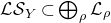 $\mathcal{LS}_Y\subset \bigoplus _\rho \mathcal{L}_\rho$
be the subsheaf of the direct sum of slab line bundles constructed in Section
3
.
$\mathcal{LS}_Y\subset \bigoplus _\rho \mathcal{L}_\rho$
be the subsheaf of the direct sum of slab line bundles constructed in Section
3
.
Denote by $\operatorname {LS}_{k^\dagger }(Y)$
the set of isomorphism classes of log structures on
$\operatorname {LS}_{k^\dagger }(Y)$
the set of isomorphism classes of log structures on $Y$
over
$Y$
over $k^\dagger$
compatible with the ggtc structure.
$k^\dagger$
compatible with the ggtc structure.
The set-theoretic function
 \begin{align*} r\colon \operatorname {LS}_{k^\dagger }(Y) \to \Gamma (Y,\mathcal{LS}_Y^\times ) \end{align*}
constructed in ( 4.15 ) is a bijection.
We prove the theorem by considering the subsheaf of regular extensions
 \begin{align*} \mathcal{E} \!{\textit {xt}}_c^1(\mathcal{M}, \mathcal{O}_Y^\times ) \subset \mathcal{E} \!{\textit {xt}}^1(\mathcal{M}, \mathcal{O}_Y^\times ) \end{align*}
that already appeared in [Reference Gross and SiebertGS06, Theorem 3.22].Footnote
9
We construct a morphism of sheaves $\varphi \colon \mathcal{LS}_Y^\times \to \mathcal{E} \!{\textit {xt}}_c^1(\mathcal{M}, \mathcal{O}_Y^\times )$
and show that it is bijective. Finally, we prove that the assignment that sends a log structure/
$\varphi \colon \mathcal{LS}_Y^\times \to \mathcal{E} \!{\textit {xt}}_c^1(\mathcal{M}, \mathcal{O}_Y^\times )$
and show that it is bijective. Finally, we prove that the assignment that sends a log structure/ $k^\dagger$
to its extension class in
$k^\dagger$
to its extension class in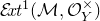 $\mathcal{E} \!{\textit {xt}}^1(\mathcal{M}, \mathcal{O}_Y^\times )$
in fact gives a bijection
$\mathcal{E} \!{\textit {xt}}^1(\mathcal{M}, \mathcal{O}_Y^\times )$
in fact gives a bijection $\operatorname {LS}_{k^\dagger } (Y)\to \Gamma \left (Y, \mathcal{E} \!{\textit {xt}}_c^1(\mathcal{M}, \mathcal{O}_Y^\times )\right )$
, and we obtain
$\operatorname {LS}_{k^\dagger } (Y)\to \Gamma \left (Y, \mathcal{E} \!{\textit {xt}}_c^1(\mathcal{M}, \mathcal{O}_Y^\times )\right )$
, and we obtain $r$
as the composition of two bijections.
$r$
as the composition of two bijections.
The content of our main theorem is not that there is some sheaf $\mathcal{LS}_Y$
with a natural identification of
$\mathcal{LS}_Y$
with a natural identification of $\operatorname {LS}_{k^\dagger } (Y)$
with
$\operatorname {LS}_{k^\dagger } (Y)$
with $\Gamma (Y, \mathcal{LS}_Y^\times )$
. Indeed, it is a basic general fact that
$\Gamma (Y, \mathcal{LS}_Y^\times )$
. Indeed, it is a basic general fact that $\operatorname {LS}_{k^\dagger } (-)$
is a sheaf. It is not even that there is some construction of a sheaf
$\operatorname {LS}_{k^\dagger } (-)$
is a sheaf. It is not even that there is some construction of a sheaf $\mathcal{LS}_Y^\times$
and a bijection from
$\mathcal{LS}_Y^\times$
and a bijection from $\operatorname {LS}_{k^\dagger } (Y)$
to
$\operatorname {LS}_{k^\dagger } (Y)$
to $\Gamma (Y, \mathcal{LS}_Y^\times )$
. Indeed, for example,
$\Gamma (Y, \mathcal{LS}_Y^\times )$
. Indeed, for example,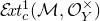 $\mathcal{E} \!{\textit {xt}}_c^1(\mathcal{M}, \mathcal{O}_Y^\times )$
is an example of such a construction.
$\mathcal{E} \!{\textit {xt}}_c^1(\mathcal{M}, \mathcal{O}_Y^\times )$
is an example of such a construction.
Our point is that the statement is true with the description of $\mathcal{LS}_Y$
given in Section 3, and that this particular description allows to construct log structures effectively. We illustrate this point here with a very simple example. (More examples can be found in Section 5.) Consider the case, see also Section 5.1, of a scheme
$\mathcal{LS}_Y$
given in Section 3, and that this particular description allows to construct log structures effectively. We illustrate this point here with a very simple example. (More examples can be found in Section 5.) Consider the case, see also Section 5.1, of a scheme $Y$
that is the union of two smooth components
$Y$
that is the union of two smooth components $Y_1$
,
$Y_1$
, $Y_2$
meeting transversally along a smooth irreducible divisor
$Y_2$
meeting transversally along a smooth irreducible divisor $D$
. We show in Section 5.1 that
$D$
. We show in Section 5.1 that
 \begin{align} \mathcal{LS}_Y \cong (N_{Y_1} D)\otimes (N_{Y_2}D), \end{align}
where $N_{Y_i} D$
denotes the normal bundle of
$N_{Y_i} D$
denotes the normal bundle of $D$
in
$D$
in $Y_i$
.Footnote
10
The description (1.2) is particularly useful when the line bundle
$Y_i$
.Footnote
10
The description (1.2) is particularly useful when the line bundle $\mathcal{LS}_Y = (N_{Y_1} D)\otimes (N_{Y_2}D)$
is not trivial, and thus it does not have a nowhere-vanishing section. Consider for example the case when
$\mathcal{LS}_Y = (N_{Y_1} D)\otimes (N_{Y_2}D)$
is not trivial, and thus it does not have a nowhere-vanishing section. Consider for example the case when $\mathcal{LS}_Y$
is, say, base point free, and let
$\mathcal{LS}_Y$
is, say, base point free, and let $Z\subset D$
be the vanishing locus of a general section
$Z\subset D$
be the vanishing locus of a general section $s\in \Gamma (D, \mathcal{LS}_Y)$
giving an isomorphism
$s\in \Gamma (D, \mathcal{LS}_Y)$
giving an isomorphism $\mathcal{O}_D(Z)\cong \mathcal{LS}_Y$
. In language introduced in Definition 5.4(1), we say that such an
$\mathcal{O}_D(Z)\cong \mathcal{LS}_Y$
. In language introduced in Definition 5.4(1), we say that such an $s$
gives a log structure/
$s$
gives a log structure/ $k^\dagger$
singular along
$k^\dagger$
singular along $Z$
. The log structure in question is the push forward to
$Z$
. The log structure in question is the push forward to $Y$
of the log smooth log structure that we have on
$Y$
of the log smooth log structure that we have on $Y\setminus Z$
. This push forward log structure is rather badly behaved, for example it is not coherent. However, it has a particularly nice log resolution. Indeed, let
$Y\setminus Z$
. This push forward log structure is rather badly behaved, for example it is not coherent. However, it has a particularly nice log resolution. Indeed, let
 \begin{align*} \widetilde {Y}_1=\operatorname {Bl}_Z Y_1 \end{align*}
be the blow up of $Z\subset Y_1$
. The strict transform of
$Z\subset Y_1$
. The strict transform of $D$
in
$D$
in $\widetilde {Y}_1$
is isomorphic to
$\widetilde {Y}_1$
is isomorphic to $D$
, so we can glue
$D$
, so we can glue $\widetilde {Y}_1$
to
$\widetilde {Y}_1$
to $Y_2$
along
$Y_2$
along $D$
to form a scheme
$D$
to form a scheme $f\colon \widetilde {Y}\to Y$
. Denoting by
$f\colon \widetilde {Y}\to Y$
. Denoting by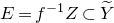 $E=f^{-1}Z\subset \widetilde {Y}$
the exceptional set, we have
$E=f^{-1}Z\subset \widetilde {Y}$
the exceptional set, we have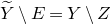 $\widetilde {Y}\setminus E=Y\setminus Z$
. It is clear that
$\widetilde {Y}\setminus E=Y\setminus Z$
. It is clear that
 \begin{multline*} N_{\widetilde {Y}_1} D=(N_{Y_1} D)(-Z), \; \text{and hence} \\ \mathcal{LS}_{\widetilde {Y}} = (N_{\widetilde {Y}_1}D)\otimes (N_{\widetilde {Y}_2}D) = \bigl ((N_{Y_1} D)\otimes (N_{Y_2}D)\bigr )(-Z) = \mathcal{LS}_Y (-Z)= \mathcal{O}_D. \end{multline*}
All of this goes to shows that there exists a unique log structure on $\widetilde {Y}$
smooth over
$\widetilde {Y}$
smooth over $k^\dagger$
and a log morphism
$k^\dagger$
and a log morphism $\widetilde {Y}^\dagger \to Y^\dagger$
over
$\widetilde {Y}^\dagger \to Y^\dagger$
over $k^\dagger$
that, when restricted to
$k^\dagger$
that, when restricted to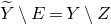 $\widetilde {Y}\setminus E=Y\setminus Z$
, is an isomorphism and so it is the log structure given by the section
$\widetilde {Y}\setminus E=Y\setminus Z$
, is an isomorphism and so it is the log structure given by the section $s\in \Gamma (Y, \mathcal{LS}_Y)$
. We call
$s\in \Gamma (Y, \mathcal{LS}_Y)$
. We call $\widetilde {Y}^\dagger \to Y^\dagger$
a log resolution.Footnote
11
$\widetilde {Y}^\dagger \to Y^\dagger$
a log resolution.Footnote
11
Our point, again, is that it would be awkward to establish these facts directly from the definition of log structure, and impossible to derive it off the shelf from the constructions and the statements in [Reference Gross and SiebertGS06] (because that paper assumes that all components of $Y$
are toric varieties). It is the independent geometric interpretation of the sheaf
$Y$
are toric varieties). It is the independent geometric interpretation of the sheaf $(N_{Y_1} D)\otimes (N_{Y_2}D)$
as the tensor product of normal bundles of
$(N_{Y_1} D)\otimes (N_{Y_2}D)$
as the tensor product of normal bundles of $D$
in
$D$
in $Y_1, Y_2$
that makes the verification straightforward, by tracking the way that normal bundles change under blow ups. Our construction of the sheaf
$Y_1, Y_2$
that makes the verification straightforward, by tracking the way that normal bundles change under blow ups. Our construction of the sheaf $\mathcal{LS}_Y$
, given in Section 3, in the two-component case immediately specializes to
$\mathcal{LS}_Y$
, given in Section 3, in the two-component case immediately specializes to $(N_{Y_1} D)\otimes (N_{Y_2}D)$
. In the general case of a ggtc space
$(N_{Y_1} D)\otimes (N_{Y_2}D)$
. In the general case of a ggtc space $Y$
, the construction is more involved, but it retains the geometric interpretation, making it possible, in many cases of interest, to construct log structures and log resolutions effectively.
$Y$
, the construction is more involved, but it retains the geometric interpretation, making it possible, in many cases of interest, to construct log structures and log resolutions effectively.
It is well known that, when $Y$
is simple normal crossings, the sheaf
$Y$
is simple normal crossings, the sheaf $\mathcal{LS}_Y$
is naturally isomorphic to
$\mathcal{LS}_Y$
is naturally isomorphic to $\mathcal{T}^1_Y=\mathcal{E} \!{\textit {xt}}^1_{\mathcal{O}_Y} (\Omega^1_Y,\mathcal{O}_Y)$
, see Theorem 5.5 and Remark 5.1 in [Reference Felten, Filip and RuddatFFR21] for further references, and so
$\mathcal{T}^1_Y=\mathcal{E} \!{\textit {xt}}^1_{\mathcal{O}_Y} (\Omega^1_Y,\mathcal{O}_Y)$
, see Theorem 5.5 and Remark 5.1 in [Reference Felten, Filip and RuddatFFR21] for further references, and so $\mathcal{LS}_Y$
is in fact a coherent sheaf in this case. However, this rather special situation is somewhat misleading because the joint condition for gluing
$\mathcal{LS}_Y$
is in fact a coherent sheaf in this case. However, this rather special situation is somewhat misleading because the joint condition for gluing $\mathcal{LS}_Y$
from line bundles happens to be linear when
$\mathcal{LS}_Y$
from line bundles happens to be linear when $Y$
is normal crossing (or a product of normal crossing spaces) while in general it is a polynomial condition that results in a non-coherent sheaf, see for example (5.3). The precise form of this polynomiality was already shown in [Reference Gross and SiebertGS06, Theorem 3.22] and in fact everything we do reduces to this explicit local description when choosing a log smooth chart of a compatible log structure.
$Y$
is normal crossing (or a product of normal crossing spaces) while in general it is a polynomial condition that results in a non-coherent sheaf, see for example (5.3). The precise form of this polynomiality was already shown in [Reference Gross and SiebertGS06, Theorem 3.22] and in fact everything we do reduces to this explicit local description when choosing a log smooth chart of a compatible log structure.
1.3 Summary of previous work
We already indicated several prior works in the semistable situation [Reference FriedmanFri83, Reference KatoKat00, Reference SteenbrinkSte95, Reference Kawamata and NamikawaKN94, Reference Schröer and SiebertSS06, Reference OlssonOls03], so we now focus on singular log structures and more general spaces. The paper [Reference Gross and SiebertGS06] is concerned with toroidal crossing spaces $Y$
that are a union of toric varieties meeting along boundary strata. Among many other things, for such a
$Y$
that are a union of toric varieties meeting along boundary strata. Among many other things, for such a $Y$
, that paper defines a sheaf
$Y$
, that paper defines a sheaf $\mathcal{LS}_Y$
and proves a natural identification
$\mathcal{LS}_Y$
and proves a natural identification $\operatorname {LS}_{k^\dagger } (Y)=\Gamma (Y, \mathcal{LS}_Y^\times )$
. Essentially,
$\operatorname {LS}_{k^\dagger } (Y)=\Gamma (Y, \mathcal{LS}_Y^\times )$
. Essentially, $\mathcal{LS}_Y$
is defined to be
$\mathcal{LS}_Y$
is defined to be $\mathcal{E} \!{\textit {xt}}_c^1(\mathcal{M}, \mathcal{O}_Y^\times ) \subset \mathcal{E} \!{\textit {xt}}^1(\mathcal{M}, \mathcal{O}_Y^\times )$
, see Sections 1.2 and 4.1, but the paper also gives an explicit local description [Reference Gross and SiebertGS06, Theorem 3.22] in terms of local functions that satisfy the joint condition, and then shows [Reference Gross and SiebertGS06, Theorem 3.28] that these local functions are sections of explicit line bundles
$\mathcal{E} \!{\textit {xt}}_c^1(\mathcal{M}, \mathcal{O}_Y^\times ) \subset \mathcal{E} \!{\textit {xt}}^1(\mathcal{M}, \mathcal{O}_Y^\times )$
, see Sections 1.2 and 4.1, but the paper also gives an explicit local description [Reference Gross and SiebertGS06, Theorem 3.22] in terms of local functions that satisfy the joint condition, and then shows [Reference Gross and SiebertGS06, Theorem 3.28] that these local functions are sections of explicit line bundles $\mathcal{N}_\rho$
(corresponding to our
$\mathcal{N}_\rho$
(corresponding to our $\mathcal{L}_\rho$
). The description of the sheaf
$\mathcal{L}_\rho$
). The description of the sheaf $\mathcal{LS}_Y$
in [Reference Gross and SiebertGS06] is sufficiently concrete to enable the effective construction of elements in
$\mathcal{LS}_Y$
in [Reference Gross and SiebertGS06] is sufficiently concrete to enable the effective construction of elements in $\operatorname {LS}_{k^\dagger }(Y)$
when
$\operatorname {LS}_{k^\dagger }(Y)$
when $Y$
is a union of toric varieties meeting along boundary strata.
$Y$
is a union of toric varieties meeting along boundary strata.
The paper [Reference Schröer and SiebertSS06] introduces the notion of Gorenstein toroidal crossing space, and goes on to study log structures on these.
1.4 Our work in relation to previous work
Our definition of ggtc space is a generalization of the Gorenstein toroidal crossing spaces of [Reference Schröer and SiebertSS06]. Our work is closely related to [Reference Schröer and SiebertSS06], but there are two important differences. The first key difference is that we work with log structures over $k^\dagger$
, where [Reference Schröer and SiebertSS06] works with absolute log structures: this change of perspective is essential to the applications that we have in mind and it results in surprising simplifications. The second key difference is that we require the Gorenstein toroidal crossing condition to hold only at the generic point of every stratum, as opposed to everywhere.
$k^\dagger$
, where [Reference Schröer and SiebertSS06] works with absolute log structures: this change of perspective is essential to the applications that we have in mind and it results in surprising simplifications. The second key difference is that we require the Gorenstein toroidal crossing condition to hold only at the generic point of every stratum, as opposed to everywhere.
Our paper generalizes the corresponding part of [Reference Gross and SiebertGS06], from toroidal crossing spaces that are union of toric varieties meeting along boundary strata, to the case of viable ggtc spaces. Here the key point of our study is a more natural and more general construction of the sheaf $\mathcal{LS}_Y$
.
$\mathcal{LS}_Y$
.
In outline, our proof follows the proof of [Reference Gross and SiebertGS06, Theorem 3.22], with changes necessary to work with our construction of the sheaf $\mathcal{LS}_Y$
. Indeed, our main innovation is the construction of the sheaf
$\mathcal{LS}_Y$
. Indeed, our main innovation is the construction of the sheaf $\mathcal{LS}_Y$
, where we use the Picard stack to show that the local descriptions of the slab bundles
$\mathcal{LS}_Y$
, where we use the Picard stack to show that the local descriptions of the slab bundles $\mathcal{L}_\rho$
, when formulated not in terms of functions but of divisors, glue automatically to give the slab bundles globally, and that the joint conditions automatically make sense globally. Unlike [Reference Gross and SiebertGS06], we never work with local charts for log structures and our approach is closer to the Deligne–Faltings view of log structures as systems of line bundles with sections.
$\mathcal{L}_\rho$
, when formulated not in terms of functions but of divisors, glue automatically to give the slab bundles globally, and that the joint conditions automatically make sense globally. Unlike [Reference Gross and SiebertGS06], we never work with local charts for log structures and our approach is closer to the Deligne–Faltings view of log structures as systems of line bundles with sections.
More detail about where exactly and how specifically we depart from [Reference Gross and SiebertGS06] can be found in the outline of the proof in Section 4.1. In particular, as was pointed out by Bernd Siebert, our point of view in the proof of Proposition 4.32, where we construct a log structure from a section of $\mathcal{LS}_Y$
, is closely related to that of [Reference Borne and VistoliBV12]. We learned that the approach via line bundle systems is also useful for recasting logarithmic data in symplectic-geometric terms, [Reference Farajzadeh-Tehrani and SwaminathanFTS25].
$\mathcal{LS}_Y$
, is closely related to that of [Reference Borne and VistoliBV12]. We learned that the approach via line bundle systems is also useful for recasting logarithmic data in symplectic-geometric terms, [Reference Farajzadeh-Tehrani and SwaminathanFTS25].
1.5 Description of contents
In Section 2 we introduce ggtc spaces. The definition is local in nature, and we take the time to describe two global objects that are naturally attached to them, the cone sheaf and the divisor system. We also introduce a property, which we call viability, that allows us to do log geometry on a ggtc space. We work in the Zariski topology for simplicity and because it is sufficient for many applications.Footnote 12
In Section 3 we explicitly construct a sheaf $\mathcal{LS}_Y$
that naturally exists on every viable ggtc space
$\mathcal{LS}_Y$
that naturally exists on every viable ggtc space $Y$
. Later in Section 4 we prove that this sheaf
$Y$
. Later in Section 4 we prove that this sheaf $\mathcal{LS}_Y$
classifies log structures on
$\mathcal{LS}_Y$
classifies log structures on $Y$
over the standard log point and compatible with the ggtc structure. In this paper, we aim to address a reader whose goal is to make a log structure on
$Y$
over the standard log point and compatible with the ggtc structure. In this paper, we aim to address a reader whose goal is to make a log structure on $Y$
explicitly. The most efficient way to do this is to construct a nowhere-vanishing global section of
$Y$
explicitly. The most efficient way to do this is to construct a nowhere-vanishing global section of $\mathcal{LS}_Y$
, and for this she only needs to know how
$\mathcal{LS}_Y$
, and for this she only needs to know how $\mathcal{LS}_Y$
is constructed; she does not need to know the proof that
$\mathcal{LS}_Y$
is constructed; she does not need to know the proof that $\mathcal{LS}_Y$
classifies log structures. Our presentation aims to facilitate explicit constructions.
$\mathcal{LS}_Y$
classifies log structures. Our presentation aims to facilitate explicit constructions.
Finally, in Section 5 we give some examples.
2. Generically Gorenstein toroidal crossing spaces
In Section 2.4 we give the formal definition of ggtc space. Basically, a ggtc space is a stratified space $Y$
such that if
$Y$
such that if $\eta \in Y$
is the generic point of a stratum, there is a fan
$\eta \in Y$
is the generic point of a stratum, there is a fan $\Sigma _\eta$
in a lattice
$\Sigma _\eta$
in a lattice $M_\eta$
and an isomorphism from the formal completion
$M_\eta$
and an isomorphism from the formal completion $\widehat {k(\eta )[\Sigma _\eta ]}$
at the origin to the formal completion
$\widehat {k(\eta )[\Sigma _\eta ]}$
at the origin to the formal completion $\widehat {\mathcal{O}_{Y,\eta }}$
at the maximal ideal. These isomorphisms need to satisfy certain coherence conditions that are best kept track of by a Kato fan in the sense of [Reference Abramovich, Chen, Marcus, Ulirsch and WiseACM+16, Section 4].
$\widehat {\mathcal{O}_{Y,\eta }}$
at the maximal ideal. These isomorphisms need to satisfy certain coherence conditions that are best kept track of by a Kato fan in the sense of [Reference Abramovich, Chen, Marcus, Ulirsch and WiseACM+16, Section 4].
In Sections 2.1–2.3 we set out carefully our notation and conventions on monoids, fans and stratified spaces: this material is elementary but tedious.
In Section 2.5 we define a property that we call viability, which allows us to do logarithmic geometry.
The definition of a ggtc space is local in nature. In Section 2.6 we define two global objects that exist on the normalization of a ggtc space, the cone sheaf and the divisor system, that enter crucially the construction of the slab bundles and the precise formulation of the joint condition.
2.1 Notation and conventions for monoids and fans
Our terminology on monoids mostly follows [Reference OgusOgu18, Chapter I]. The following summary of terminology and notation is intended for reference, not as a complete dictionary on monoids.
Convention 2.1.
-
(1) A $\textit{lattice}$
is a free abelian group
$M\cong \mathbb{Z}^r$
of finite rank
$r$
. We denote
$M_{\mathbb{R}}:=M\otimes _{\mathbb{Z}}\mathbb{R}$
.
$\textit{lattice}$
is a free abelian group
$M\cong \mathbb{Z}^r$
of finite rank
$r$
. We denote
$M_{\mathbb{R}}:=M\otimes _{\mathbb{Z}}\mathbb{R}$
. -
(2) A
$\textit{monoid}$
is a commutative semigroup with neutral element. Our default position is to denote the operation and unit of a monoid additively by
$+$
,
$0$
. (If
$R$
is a ring, for example, we may want to consider the monoid
$(R,\times , 1)$
.) -
(3) If
$M$
is a lattice and
$S\subset M$
a subset, we denote by
$\langle S \rangle$
the saturation in
$M$
of the subgroup generated by
$S$
and by
$\langle S \rangle _+$
the saturation in
$M$
of the submonoid generated by
$S$
. Similarly, if
$\tau \subset M_{\mathbb{R}}$
, we denote
$\langle \tau \rangle :=\langle \tau \cap M \rangle$
and
$\langle \tau \rangle _+:=\langle \tau \cap M \rangle _+$
. -
(4) The group of units of a monoid
$P$
is denoted by
$P^\times$
. A monoid
$P$
is
$\textit{sharp}$
if
$P^\times =(0)$
. -
(5) A monoid
$P$
is
$\textit{toric}$
if there exist a lattice
$M$
of finite rank and a closed convex rational polyhedral cone
$\sigma \subset M_{\mathbb{R}}$
such that
$P=\sigma \cap M$
. In this paper we often work with toric monoids and we almost always assume them to be sharp. -
(6) Let
$P$
be a monoid. A submonoid
$F\subset P$
is a
$\textit{face}$
if the following condition is satisfied. For all
$u, v\in P$
, if
$u+v\in F$
, then
$u,v\in F$
. We write
$F\leqslant P$
to mean that
$F$
is a face of
$P$
. The notation
$F\lt P$
means that
$F$
is a proper face of
$P$
, that is,
$F$
is a face and
$F\neq P$
. -
(7) When
$F\leqslant P$
we denote by
$F^{-1} P$
the
$\textit{localization}$
of
$P$
at
$F$
. We call the monoid homomorphism
$P\to F^{-1} P$
a face localization. When
$F\leqslant P$
, the
$\textit{quotient}$
$P/F$
is the monoid
$F^{-1} P/F$
. We call the monoid homomorphism
$P\to P/F$
a face quotient.
-
(8) If
$P$
is a monoid and
$\textbf {1}\in P$
an element, we use
$P/\textbf {1}$
denote the quotient of
$P$
by the submonoid generated by
$\textbf {1}$
. For example
$\mathbb{N}^2/(1,1)\cong \mathbb{Z}$
. -
(9) If
$P$
is a monoid, we denote by
$P^{\operatorname {gp}}$
the universal (Grothendieck) group of
$P$
. -
(10) If
$R$
is a ring and
$P$
a monoid, we denote by
$R[P]$
the monoid ring.









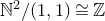


Definition 2.2. Let $M\cong \mathbb{Z}^r$
be a lattice.
$M\cong \mathbb{Z}^r$
be a lattice.
-
(1) A fan in
$M$
is a finite set
$\Sigma$
of closed convex rational polyhedral cones in
$M_{\mathbb{R}}$
such that:-
(i) for all
$\tau \in \Sigma$
, if
$\mu \leqslant \tau$
is a face, then
$\mu \in \Sigma$
; -
(ii) for all
$\tau , \mu \in \Sigma$
,
$\tau \cap \mu$
is a face of both
$\tau$
and
$\mu$
.
The
$\textit{support}$
of the fan, denoted by
$|\Sigma |\subset M_{\mathbb{R}}$
, is the union of the cones of
$\Sigma$
.The fan is said to be
$\textit{complete}$
if
$|\Sigma |=M_{\mathbb{R}}$
. -
-
(2) Let
$\Sigma$
be a fan and
$\rho \in \Sigma$
a cone.-
(a) The
$\textit{localization}$
$\rho ^{-1}\Sigma$
of
$\Sigma$
in
$\rho$
is the fan in
$M$
that consists of the convex cones
$\sigma -\rho =\{x-y\in M_{\mathbb{R}}|x\in \sigma ,y\in \rho \}$
where
$\sigma$
ranges over all cones in
$\Sigma$
that contain
$\rho$
. -
(b) The
$\textit{quotient}$
$\Sigma /\rho$
of
$\Sigma$
by
$\rho$
is the fan in
$M/\langle \rho \rangle$
obtained from the localization
$\rho ^{-1}\Sigma$
by projecting each of its cones under the linear map
$M\to M/\langle \rho \rangle$
.
-
-
(3) If
$\Sigma$
is a fan in
$M$
and
$R$
is a ring, the
$\textit{Stanley}{-}\textit{Reisner ring}$
$R[\Sigma ]$
is the free
$R$
-module over the symbols
$z^m$
for those
$m\in M$
which are also contained in some cone of
$\Sigma$
, with multiplication defined byWe denote by
\begin{align*} z^m\cdot z^{m'}=\left \{ \begin{array}{ll} z^{m+m'} & \hbox{if there is a cone }\sigma \in \Sigma \hbox{ that contains }m,m',\\ 0 & \hbox{otherwise.}\end{array}\right. \end{align*}
$\mathfrak{m}$
the ideal generated by all the symbols
$z^{m}$
with
$m\neq 0$
. If
$R$
is a field,
$\mathfrak{m}$
is a maximal ideal.








Lemma 2.3. There is an equivalence between the following two categories.
-
(1) The category with objects pairs
$(P, {\bf 1})$
of a sharp toric monoid
$P$
and an element
${\bf 1}\in P$
such that
$P \setminus ({\bf 1}+P)$
is the union of the proper faces of
$P$
, and morphisms face quotients.
-
(2) The category whose objects are pairs
$(\Sigma , \varphi )$
of a rational polyhedral fan
$\Sigma$
, not necessarily complete but with convex support, and a polarization, that is, a strictly convex piecewise linear function
$\varphi \colon \vert \Sigma \vert \cap M \to \mathbb{Z}$
up to the addition of an integral linear function
$M\to \mathbb{Z}$
, and morphisms fan quotients.




Under this equivalence,
 \begin{align*} P\setminus ({\bf 1}+P)= \cup _{F\lt P} F \end{align*}
if and only if the fan $\Sigma$
is complete.
$\Sigma$
is complete.
In addition, under this equivalence, $\mathbb{Z}[P]/(z^{\textbf {1}})=\mathbb{Z}[\Sigma ]$
.
$\mathbb{Z}[P]/(z^{\textbf {1}})=\mathbb{Z}[\Sigma ]$
.
Sketch of Proof.
Starting from $(\Sigma , \varphi )$
, let
$(\Sigma , \varphi )$
, let $P$
be the supergraph of
$P$
be the supergraph of $\varphi$
in
$\varphi$
in $M \oplus \mathbb{Z}$
and
$M \oplus \mathbb{Z}$
and $\textbf {1}=(0,1)$
.
$\textbf {1}=(0,1)$
.
Vice versa, starting from $(P, {\bf 1})$
, let
$(P, {\bf 1})$
, let $M$
be the universal group of the quotient monoid
$M$
be the universal group of the quotient monoid $P /{\bf 1}$
of
$P /{\bf 1}$
of $P$
by the congruence relation generated by the submonoid
$P$
by the congruence relation generated by the submonoid ${\bf 1}\mathbb{N}$
, and let
${\bf 1}\mathbb{N}$
, and let $\Sigma$
be the fan in
$\Sigma$
be the fan in $M$
whose cones are the projections under the obvious homomorphism
$M$
whose cones are the projections under the obvious homomorphism $P\to M$
of the proper faces of
$P\to M$
of the proper faces of $P$
that do not contain
$P$
that do not contain ${\bf 1}$
.
${\bf 1}$
.
2.2 Notation and conventions for stratified spaces
The next two definitions correspond to the notion of finite partition of [Sta26], Tag 09XZ and finite good stratification of [Sta26], Tag 09Y0.
Definition 2.4. Let $X$
be a topological space. A partition of
$X$
be a topological space. A partition of $X$
is a decomposition
$X$
is a decomposition
 \begin{align*} X=\coprod _{\eta \in T} X_\eta ^\star \end{align*}
into locally closed subsets $X_\eta$
indexed by a finite set
$X_\eta$
indexed by a finite set $T$
. The
$T$
. The $X_\eta ^\star$
are called the parts of the partition.
$X_\eta ^\star$
are called the parts of the partition.
We denote by $X_\eta =\overline {X_\eta ^\star }$
the closure of
$X_\eta =\overline {X_\eta ^\star }$
the closure of $X_\eta ^\star$
.
$X_\eta ^\star$
.
Definition 2.5. Let $X$
be a topological space. A good stratification of
$X$
be a topological space. A good stratification of $X$
is a partition
$X$
is a partition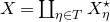 $X=\coprod _{\eta \in T}X_\eta ^\star$
such that for all
$X=\coprod _{\eta \in T}X_\eta ^\star$
such that for all $\mu , \eta \in T$
we have
$\mu , \eta \in T$
we have
 \begin{align*} X_\mu ^\star \cap X_\eta \neq \emptyset \quad \Rightarrow \quad X_\mu ^\star \subset X_\eta. \end{align*}
The $X_\eta ^\star$
are called the strata of the stratification.
$X_\eta ^\star$
are called the strata of the stratification.
Given a good stratification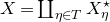 $X=\coprod _{\eta \in T}X_\eta ^\star$
, we obtain a partial ordering on the index set
$X=\coprod _{\eta \in T}X_\eta ^\star$
, we obtain a partial ordering on the index set $T$
by setting
$T$
by setting $\mu \leqslant \eta$
if and only if
$\mu \leqslant \eta$
if and only if $X_\mu ^\star \subset X_\eta$
. It then follows that
$X_\mu ^\star \subset X_\eta$
. It then follows that
 \begin{align*} X_\eta = \coprod _{\mu \leqslant \eta }X_\mu ^\star. \end{align*}
Definition 2.6.
-
(1) A space is a scheme or Deligne–Mumford stack of finite type over
$k$
. -
(2) A stratified space is a space
$Y$
endowed with a good stratificationsuch that all strata are irreducible. Under this assumption,
\begin{align*} Y=\coprod _{\eta \in T} Y_\eta ^\star \end{align*}
$T$
is identified with the set of generic points of the strata, and the partial ordering on
$T$
is induced by specialization: for all
$\eta _1,\eta _2\in T$
,
$\eta _1\leqslant \eta _2$
if and only if
$\eta _1$
is a specialization of
$\eta _2$
.
When
$Y$
is a Deligne–Mumford stack, we assume in addition that the generic points of strata have trivial stabilizers. -
(3) The codimension of
$\eta \in T$
is the codimension in
$Y$
of the corresponding stratum. We denote by
$T^{[i]}\subset T$
the set of points of codimension
$i$
and we write
\begin{align*} Y^{[i]}=\coprod _{\eta \in T^{[i]}} Y_\eta , \qquad Y^{(i)}=\bigcup _{\eta \in T^{[i]}} Y_\eta. \end{align*}


Lemma 2.7.
Let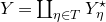 $Y=\coprod _{\eta \in T} Y_\eta ^\star$
be a stratified space.
$Y=\coprod _{\eta \in T} Y_\eta ^\star$
be a stratified space.
The subset topology of $T\subset Y$
is the order topology:
$T\subset Y$
is the order topology: $W\subset T$
is open if and only if for all
$W\subset T$
is open if and only if for all $\tau _1 \in W$
, if
$\tau _1 \in W$
, if $\tau _2\geqslant \tau _1$
then
$\tau _2\geqslant \tau _1$
then $\tau _2\in W$
. We have the following.
$\tau _2\in W$
. We have the following.
-
(i) For all
$\eta \in T$
,is the smallest open subset of
\begin{align*} T_{\geqslant \eta } = \{\mu \in T \mid \mu \geqslant \eta \} \end{align*}
$T$
that contains
$\eta$
;
-
(ii) The inclusion
defined such that
\begin{align*} a\colon T \hookrightarrow Y \quad \textit{has a continuous retraction} \quad b\colon Y\to T \end{align*}
$b(y)=\eta$
if
$y\in Y^\star _\eta$
;
-
(iii) The map
$b$
is open and for all Zariski open subset
$U\subset Y$
,
$b(U)=a^{-1}(U)=U\cap T$
.



Sketch of Proof.
The map $b$
is continuous: indeed for all
$b$
is continuous: indeed for all $\eta \in T$
we have that
$\eta \in T$
we have that
 \begin{align*} b^{-1} (T_{\geqslant \eta })=\{y\in Y \mid b(y)\geqslant \eta \}=\coprod _{\mu \geqslant \eta } Y_\mu ^\star \end{align*}
is the union of all locally closed strata that have $\eta$
in their Zariski closure and hence it is Zariski open in
$\eta$
in their Zariski closure and hence it is Zariski open in $Y$
.
$Y$
.
Consider a Zariski open subset $U\subset Y$
. If
$U\subset Y$
. If $\eta \in b(U)$
, then that means that
$\eta \in b(U)$
, then that means that $Y_\eta ^\star \cap U \neq \emptyset$
, or, equivalently, that
$Y_\eta ^\star \cap U \neq \emptyset$
, or, equivalently, that $\eta \in U$
. This shows that
$\eta \in U$
. This shows that $b(U)=a^{-1}(U)$
and in particular it is open.
$b(U)=a^{-1}(U)$
and in particular it is open.
Definition 2.8. Let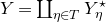 $Y=\coprod _{\eta \in T} Y_\eta ^\star$
be a stratified space. For all
$Y=\coprod _{\eta \in T} Y_\eta ^\star$
be a stratified space. For all $\eta \in T$
, the open star of
$\eta \in T$
, the open star of $\eta$
is the Zariski open subset
$\eta$
is the Zariski open subset
 \begin{align*} U_\eta =\{y\in Y \mid b(y) \geqslant \eta \} = b^{-1}(T_{\geqslant \eta }) \subset Y, \end{align*}
that is, the union of all strata of $Y$
that have
$Y$
that have $\eta$
in their Zariski closure.
$\eta$
in their Zariski closure.
Corollary 2.9.
In the situation of Lemma 2.7
, if $\mathcal{F}$
is a sheaf on
$\mathcal{F}$
is a sheaf on $T$
, then the sheaves
$T$
, then the sheaves $a_\star \mathcal{F}$
and
$a_\star \mathcal{F}$
and $b^{-1} \mathcal{F}$
on
$b^{-1} \mathcal{F}$
on $Y$
are isomorphic.
$Y$
are isomorphic.


2.3 The basic setup and assumptions for toroidal crossing spaces
In what follows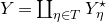 $Y=\coprod _{\eta \in T} Y_\eta ^\star$
is a stratified space satisfying the following assumptions:
$Y=\coprod _{\eta \in T} Y_\eta ^\star$
is a stratified space satisfying the following assumptions:
-
(1)
$Y$
is reduced, equidimensional, and the irreducible components of
$Y$
are normal; -
(2)
$Y$
is normal crossing in codimension
$1$
; denoting bythe normalization, the restriction of
\begin{align*} \varepsilon \colon Y^{[0]}=\coprod _{\sigma \in T^{[0]}} Y_\sigma \longrightarrow Y \end{align*}
$\varepsilon$
to to
$\varepsilon ^{-1}(Y^{(1)}\setminus Y^{(2)})$
is a degree-two disconnected finite étale cover over each component of the target;
-
(3)
$Y$
is the push-out of the diagram of spaces
$Y^{[1]} \rightrightarrows Y^{[0]}$
where the two maps are obtained from the inclusions
$Y_\rho \to Y_{\sigma }$
,
$Y_\rho \to Y_{\sigma '}$
.





2.4 Generically Gorenstein toroidal crossing space
Setup 2.11. We introduce objects and notation that are used in Definition 2.12.
Fix a finite poset $T$
equipped with the order topology.
$T$
equipped with the order topology.
-
(1) To give a sheaf of monoids
$\mathcal{P}$
on
$T$
is equivalent to give the following data subject to obvious compatibilities:-
(i) for all
$\eta \in T$
a monoid
$P_\eta$
; and -
(ii) for all
$\eta _1\le \eta _2$
, a generization homomorphism
\begin{align*} P_{\eta _1} \to P_{\eta _2}. \end{align*}
-
-
(2) A Kato fan [Reference Abramovich, Chen, Marcus, Ulirsch and WiseACM+16, Section 4] is a sharp monoidal space that is locally isomorphic to
$\operatorname {Spec} P$
,
$P$
a sharp toric monoid. Let
$\mathcal{P}$
be a sheaf of monoids on
$T$
making
$T$
a Kato fan. In particular, all the
$P_\eta$
are sharp toric monoids, and all the generization homomorphisms are face quotients. It follows from the definition that, for all
$\eta \in T$
, there is a bijective identification of the poset of faces of
$P_\eta$
with
$\{\tau \in T \mid \tau \geqslant \eta \}$
. -
(3) Given a Kato fan
$(T,\mathcal{P})$
, consider a global section
${\bf 1}\in \Gamma (T, \mathcal{P})$
corresponding to the datum, for all
$\eta \in T$
, of sections
${\bf 1}_\eta \in P_\eta$
such that
$P_\eta \setminus ( {\bf 1}_\eta + P_\eta )$
is the union of all the proper faces of
$P_\eta$
. In this situation, by Lemma 2.3, the pair
$(\mathcal{P},{\bf 1})$
gives rise to a sheaf of complete fans
${\bf \Sigma\ }$
in the sheaf of lattices
$\mathcal{M}=\mathcal{P}/{\bf 1}$
. This unpacks in the data, for all
$\eta \in T$
, of a fan
$\Sigma _\eta$
in
$M_\eta = P_\eta /{\bf 1}_\eta$
, and for all
$\eta _1 \leqslant \eta _2$
generization maps (viewing
$\eta _2\in \Sigma _{\eta _1}$
) quotient homomorphisms
$M_{\eta _1}\to M_{\eta _2}=M_{\eta _1}/\langle \eta _2\rangle$
identifying
$\Sigma _{\eta _2}$
with the quotient fan
$\Sigma _{\eta _1}/\eta _2$
. For all
$\eta \in T$
, the poset of faces of
$P_\eta$
is identified with the fan
$\Sigma _\eta$
, and this induces an identification:
\begin{align*} \Sigma _\eta =\{ \tau \in T \mid \tau \geqslant \eta \}. \end{align*}











Now fix a stratified space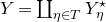 $Y=\coprod _{\eta \in T} Y_\eta ^\star$
satisfying the assumptions of Section 2.3. Assume that
$Y=\coprod _{\eta \in T} Y_\eta ^\star$
satisfying the assumptions of Section 2.3. Assume that $T$
is endowed with a pair
$T$
is endowed with a pair $(\mathcal{P}, {\bf 1})$
of a sheaf of monoids
$(\mathcal{P}, {\bf 1})$
of a sheaf of monoids $\mathcal{P}$
making
$\mathcal{P}$
making $T$
a Kato fan and global section
$T$
a Kato fan and global section ${\bf 1}\in \Gamma (Y,\mathcal{P})$
as in part (3).
${\bf 1}\in \Gamma (Y,\mathcal{P})$
as in part (3).
-
(4) Fix
$\eta \in T$
. The space
$\operatorname {Spec} k(\eta )[\Sigma _\eta ]$
has a natural stratification indexed by the cones of
$\Sigma _\eta$
ordered by inclusion. For a cone
$\tau \in \Sigma _\eta$
we denote by
$O_\tau \subset \operatorname {Spec} k(\eta )[\Sigma _\eta ]$
the corresponding stratum. For all
$\tau _1,\tau _2\in \Sigma _\eta$
,
$\tau _1\leqslant \tau _2$
if and only if
$O_{\tau _1}\subset \overline {O}_{\tau _2}$
. We denote by
$ \widehat {k(\eta )[\Sigma _\eta ]}$
the formal completion at the origin, and, for all
$\tau \geqslant \eta$
, we denote by
$\widehat {O_{\tau }}\subset \operatorname {Spec} \widehat {k(\eta )[\Sigma _\eta ]}$
the induced subscheme. -
(5) Fix
$\eta \in T$
. The local ring
$(\mathcal{O}_{Y,\eta },\mathfrak{m}_\eta )$
of
$Y$
is a local Noetherian
$k$
-algebra (
$k$
is the base field) with residue field
$k(\eta )$
. We denote by
$\widehat {\mathcal{O}_{Y,\eta }}$
the formal completion at
$\mathfrak{m}_{\eta }$
. By the Cohen structure theorem [Sta26],
Tag 032A
$\widehat {\mathcal{O}_{Y,\eta }}$
contains a field isomorphic to
$k(\eta )$
. For all
$\tau \geqslant \eta$
, we denote by
$\widehat {Y_\tau }\subset \operatorname {Spec} \widehat {\mathcal{O}_{Y,\eta }}$
the induced subscheme.










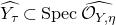
Definition 2.12. Importing Setup 2.11, a ggtc space is a tuple
 \begin{align*} \bigg( Y=\coprod _{\eta \in T} Y_\eta ^\star ,(\mathcal{P}, {\bf 1}),\{\widehat {f_\eta }\mid \eta \in T\}\bigg) \end{align*}
of a stratified space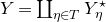 $Y=\coprod _{\eta \in T} Y_\eta ^\star$
satisfying the assumptions of Section 2.3, and we have the following.
$Y=\coprod _{\eta \in T} Y_\eta ^\star$
satisfying the assumptions of Section 2.3, and we have the following.
-
(a) A pair
$(\mathcal{P}, {\bf 1})$
of a Zariski sheaf
$\mathcal{P}$
of monoids on
$T$
making
$T$
a Kato fan, and a global section
${\bf 1}\in \Gamma (T, \mathcal{P})$
given by elements
${\bf 1}_\eta \in P_\eta$
such that
$P_\eta \setminus ({\bf 1}_\eta + P_\eta )$
is the union of all the proper faces of
$P_\eta$
. The section
${\bf 1}$
induces a sheaf of complete fans
${\bf \Sigma\ }$
in the sheaf of lattices
$\mathcal{M}=\mathcal{P}/{\bf 1}$
. -
(b) For all
$\eta \in T$
, a ring isomorphism:
\begin{align*} \widehat {f_\eta }\colon \widehat {k(\eta )[\Sigma _\eta ]} \overset {\cong }{\longrightarrow } \widehat {\mathcal{O}_{Y, \eta }} \, , \end{align*}





subject to the following condition: for all $\tau \in \Sigma _\eta$
, the isomorphism
$\tau \in \Sigma _\eta$
, the isomorphism $\widehat {f_\eta }$
identifies
$\widehat {f_\eta }$
identifies $\widehat {Y_\tau ^\star }$
with
$\widehat {Y_\tau ^\star }$
with $\widehat {O_\tau }$
.
$\widehat {O_\tau }$
.
The sheaf $\mathcal{P}$
is called the ghost sheaf of the ggtc space;
$\mathcal{P}$
is called the ghost sheaf of the ggtc space; $\mathcal{M}$
the relative ghost sheaf;
$\mathcal{M}$
the relative ghost sheaf; $\widehat {f_\eta }$
the local formal frames.
$\widehat {f_\eta }$
the local formal frames.
Convention 2.13. Sometimes for simplicity we write ‘let $Y$
be a ggtc space’. When we do this, it is understood that
$Y$
be a ggtc space’. When we do this, it is understood that $Y$
is a stratified space, and that it has a ghost sheaf, a relative ghost sheaf, etc., and we take it for granted that they will be denoted by
$Y$
is a stratified space, and that it has a ghost sheaf, a relative ghost sheaf, etc., and we take it for granted that they will be denoted by $\mathcal{P}$
,
$\mathcal{P}$
, $\mathcal{M}$
, etc.
$\mathcal{M}$
, etc.
Remark 2.14.
-
(1) The reader should not be overly concerned about the formal local frames. We could replace part (b) with the following (possibly more familiar) requirement: for all
$\eta \in T$
, there is a Zariski closed subset
$Z_\eta \subsetneq Y_\eta ^\star$
such that, for all
$y\in Y_\eta \setminus Z_\eta$
, there is a neighbourhood
$y\in W \subset Y_\eta \setminus Z_\eta$
and a smooth morphismThese morphisms would have to satisfy a more-or-less obvious coherence condition.
\begin{align*} W \to \operatorname {Spec} k[\Sigma _\eta ]. \end{align*}
-
(2) Let
$Y$
be a ggtc space. For all
$\eta \in T$
,
$\operatorname {Spec} \mathbb{Z}[P_\eta ]$
is a Gorenstein toric variety with reduced boundary
$B=\operatorname {div} z^{{\bf 1}}$
. -
(3) In [Reference Schröer and SiebertSS06] ‘gtc’ is an acronym of ‘Gorenstein toroidal crossing’ in the étale topology. On the one hand, in this paper, we work in the Zariski topology. On the other hand, we only require a Gorenstein toroidal crossing structure at the generic points of strata.





Example 2.15. In many applications of interest,Footnote
13
the formal frame isomorphisms $\widehat {f_\eta }\colon \widehat {k(\eta )[\Sigma _\eta ]} \overset {\cong }{\longrightarrow } \widehat {\mathcal{O}_{Y,\eta }}$
arise from bona fide frame isomorphisms
$\widehat {f_\eta }\colon \widehat {k(\eta )[\Sigma _\eta ]} \overset {\cong }{\longrightarrow } \widehat {\mathcal{O}_{Y,\eta }}$
arise from bona fide frame isomorphisms
 \begin{align*} f_\eta \colon k(\eta )[\Sigma _\eta ]_{\mathfrak{m}} \overset {\cong }{\longrightarrow } \mathcal{O}_{Y,\eta }. \end{align*}
In general, however, this is not possible. Consider, for example, a situation where $Y=Y_1\cup Y_2$
is a union of two smooth elliptic curves that meet in a point
$Y=Y_1\cup Y_2$
is a union of two smooth elliptic curves that meet in a point $P$
with residue field
$P$
with residue field $k=k(P)$
. The discrete valuation ring of
$k=k(P)$
. The discrete valuation ring of $P$
in either component is not isomorphic to
$P$
in either component is not isomorphic to $k[x]_{(x)}$
.
$k[x]_{(x)}$
.
2.5 Viable ggtc spaces
In this section we define the key notion of viability of a ggtc space.
Definition 2.16. Fix a ggtc space $\bigl ( Y=\coprod _{\eta \in T} Y_\eta ^\star ,(\mathcal{P}, {\bf 1}),\{\widehat {f_\eta }\mid \eta \in T\}\bigr )$
.
$\bigl ( Y=\coprod _{\eta \in T} Y_\eta ^\star ,(\mathcal{P}, {\bf 1}),\{\widehat {f_\eta }\mid \eta \in T\}\bigr )$
.
For all $\eta \in T$
,
$\eta \in T$
, $\operatorname {Spec} k(\eta )[\Sigma _\eta ]$
has a stratification with strata
$\operatorname {Spec} k(\eta )[\Sigma _\eta ]$
has a stratification with strata $\{O_\tau ^\star \mid \tau \in \Sigma _\eta \}$
,
$\{O_\tau ^\star \mid \tau \in \Sigma _\eta \}$
, $O_\tau =\overline {O_\tau ^\star }$
. For
$O_\tau =\overline {O_\tau ^\star }$
. For $\tau \in \Sigma _\eta$
, denote by
$\tau \in \Sigma _\eta$
, denote by
 \begin{align*} \Omega _\tau = \coprod _{\tau \leqslant \tau ^\prime } O_{\tau ^\prime }^\star \end{align*}
the open star of $\tau$
, and denote by
$\tau$
, and denote by $\overline {\Omega }_\tau$
its Zariski closure. In addition, denote by
$\overline {\Omega }_\tau$
its Zariski closure. In addition, denote by
 \begin{align*} \operatorname {Div}^+_\flat \overline {\Omega }_\tau \end{align*}
the monoid of effective Cartier divisors on $\overline {\Omega }_\tau$
supported on
$\overline {\Omega }_\tau$
supported on $\textstyle\bigcup _{\rho \in T^{[1]}} O_\rho$
.
$\textstyle\bigcup _{\rho \in T^{[1]}} O_\rho$
.
For $\tau \in \Sigma _\eta$
and
$\tau \in \Sigma _\eta$
and $m\in \tau \cap M_\eta$
, denote by
$m\in \tau \cap M_\eta$
, denote by $z^m\in k(\eta )[\Sigma _\eta ]$
the corresponding monomial. For all
$z^m\in k(\eta )[\Sigma _\eta ]$
the corresponding monomial. For all $\tau \in \Sigma _\eta$
we have a monoid homomorphism
$\tau \in \Sigma _\eta$
we have a monoid homomorphism
 \begin{align*} \operatorname {div}_{\eta ,\tau } \colon \langle \tau \rangle _+ \ni m \mapsto \operatorname {div} z^m \in \operatorname {Div}^+_\flat \overline {\Omega }_\tau. \end{align*}
For $m\in \langle \tau \rangle _+$
, write
$m\in \langle \tau \rangle _+$
, write $\operatorname {div}_{\eta ,\tau } (m) = \sum _{\rho \in T^{[1]}} m_\rho O_\rho$
and consider the effective divisor:
$\operatorname {div}_{\eta ,\tau } (m) = \sum _{\rho \in T^{[1]}} m_\rho O_\rho$
and consider the effective divisor:
 \begin{align*} D_{\eta ,\tau } (m)=\sum _{\rho \in T^{[1]}} m_{\rho} Y_{\rho} \quad \text{on $\overline{U}_\tau \cap U_\eta $}. \end{align*}
We say that the ggtc space is viable if, for all $\eta \in T$
, for all
$\eta \in T$
, for all $\tau \in \Sigma _\eta$
and
$\tau \in \Sigma _\eta$
and $m\in \tau \cap M_\eta$
as above, the divisor
$m\in \tau \cap M_\eta$
as above, the divisor $D_{\eta ,\tau } (m)$
is a Cartier divisor.
$D_{\eta ,\tau } (m)$
is a Cartier divisor.
Notation 2.17. Let $Y$
be a viable ggtc space. For all
$Y$
be a viable ggtc space. For all $\eta \in T$
and
$\eta \in T$
and $\tau \in \Sigma _\eta$
, we denote by
$\tau \in \Sigma _\eta$
, we denote by
 \begin{align*} D_{\eta , \tau } \colon \langle \tau \rangle _+ \to \operatorname {Div}^+_\flat \bigl ( \overline {U}_\tau \cap U_\eta \bigr ) \end{align*}
the monoid homomorphism provided by Definition 2.16.
The monoid homomorphism $D_{\eta , \tau }$
extends to a group homomorphism that, abusing notation, we still denote by
$D_{\eta , \tau }$
extends to a group homomorphism that, abusing notation, we still denote by $D_{\eta , \tau } \colon \langle \tau \rangle \to \operatorname {Div}_\flat \bigl ( \overline {U}_\tau \cap U_\eta \bigr )$
.
$D_{\eta , \tau } \colon \langle \tau \rangle \to \operatorname {Div}_\flat \bigl ( \overline {U}_\tau \cap U_\eta \bigr )$
.
Remark 2.18. In the situation of Definition 2.16, for all ggtc spaces, not necessarily viable, it can be shown that for all $\eta \in T$
,
$\eta \in T$
, $\tau \in \Sigma _\eta$
and
$\tau \in \Sigma _\eta$
and $m\in \tau \cap M_\eta$
, there is a Zariski neighbourhood
$m\in \tau \cap M_\eta$
, there is a Zariski neighbourhood
 \begin{align*} \eta \subset W \subset \overline {U}_\tau \cap U_\eta \end{align*}
such that $D_{\eta ,\tau } (m)$
is Cartier on
$D_{\eta ,\tau } (m)$
is Cartier on $W$
.
$W$
.
Example 2.19. Consider $r,a\gt 0$
with
$r,a\gt 0$
with $\gcd (r,a)=1$
and
$\gcd (r,a)=1$
and $\operatorname {char}(k)\nmid r$
. The natural ggtc structure on the
$\operatorname {char}(k)\nmid r$
. The natural ggtc structure on the $3$
-dimensional Deligne–Mumford stack
$3$
-dimensional Deligne–Mumford stack
 \begin{align*} Y=(uv=0)\subset [\mathbb{A}^4/\mu _r]\, , \end{align*}
where $u,v,w,z$
are coordinates on
$u,v,w,z$
are coordinates on $\mathbb{A}^4$
and
$\mathbb{A}^4$
and $\mu _r$
acts with weights
$\mu _r$
acts with weights $(1,-1,a,-a)$
is viable, as we now explain. By assumption, there is an integer
$(1,-1,a,-a)$
is viable, as we now explain. By assumption, there is an integer $s$
so that
$s$
so that $sa=r-1$
modulo
$sa=r-1$
modulo $r$
. This is one of those cases where the formal frames arise from bona fide frame isomomorphisms: an example of a frame at
$r$
. This is one of those cases where the formal frames arise from bona fide frame isomomorphisms: an example of a frame at $\eta =(u,v)$
is the isomorphism
$\eta =(u,v)$
is the isomorphism
 \begin{align*}f_\eta \colon \left (k(\eta )[x,y]/(xy)\right )_{(x,y)}\to \mathcal{O}_{Y,\eta }, \quad x\mapsto uw^s,\ y\mapsto vz^s.\end{align*}
There are other possibilities for frame maps. We could post-compose this frame with any equivariant change of coordinates at $\eta$
that preserves strata, e.g.,
$\eta$
that preserves strata, e.g., $u\mapsto uw^{i}z^{j}$
,
$u\mapsto uw^{i}z^{j}$
, $v\mapsto vw^{k}z^{l}$
with
$v\mapsto vw^{k}z^{l}$
with $(i-j)$
and
$(i-j)$
and $(k-l)$
divisible by
$(k-l)$
divisible by $r$
, so there is a variety of choices.
$r$
, so there is a variety of choices.
Most importantly for the ggtc property, the divisor $\operatorname {div}(f_\eta (x))$
equals
$\operatorname {div}(f_\eta (x))$
equals $\operatorname {div} (u)$
in
$\operatorname {div} (u)$
in $\operatorname {Spec}\mathcal{O}_{Y,\eta }$
and therefore extends as a Cartier divisor in the component
$\operatorname {Spec}\mathcal{O}_{Y,\eta }$
and therefore extends as a Cartier divisor in the component $(v=0)\subset Y$
, supported on
$(v=0)\subset Y$
, supported on $(u=v=0)$
, even at
$(u=v=0)$
, even at $y=(0,0,0,0)\in (v=0)$
. Indeed, because we are working with the Deligne–Mumford stack
$y=(0,0,0,0)\in (v=0)$
. Indeed, because we are working with the Deligne–Mumford stack $Y$
, rather than its coarse moduli space, the divisors
$Y$
, rather than its coarse moduli space, the divisors $ \operatorname {div} (u), \operatorname {div} (v)$
are well-defined Cartier divisors, also at the point
$ \operatorname {div} (u), \operatorname {div} (v)$
are well-defined Cartier divisors, also at the point $y=(0,0,0,0)\in Y$
: even though the functions
$y=(0,0,0,0)\in Y$
: even though the functions $u,v$
are not well-defined, each gives rise to a descent datum for a Cartier divisor from
$u,v$
are not well-defined, each gives rise to a descent datum for a Cartier divisor from $\mathbb{A}^4$
to
$\mathbb{A}^4$
to $Y$
. These divisors are not Cartier on the coarse moduli on the other hand.
$Y$
. These divisors are not Cartier on the coarse moduli on the other hand.
This example turns up very frequently in applications to smoothing toric Fano varieties, and it is precisely to allow for this example that we need to be working with log structures on ggtc Deligne–Mumford stacks, as opposed to just ggtc schemes.
The coarse moduli scheme of $Y$
is a ggtc scheme that is not viable if
$Y$
is a ggtc scheme that is not viable if $r\gt 1$
.
$r\gt 1$
.
Example 2.20. It is easy to construct examples of ggtc spaces that are not toroidal crossing spaces. For example, assume $f,g,h$
are mutually coprime and glue
$f,g,h$
are mutually coprime and glue
 \begin{align*}X_1=\left (y g(x_1, \ldots , x_n)+f(x_1, \ldots x_n)=0\right )\subset \mathbb{A}^{n+1},\end{align*}
 \begin{align*}X_2= \left (z h(x_1, \ldots , x_n)+f(x_1, \ldots x_n)=0\right )\subset \mathbb{A}^{n+1}\end{align*}
along the common subvariety $\left ( f(x_1,\ldots , x_n)=0\right )\subset \mathbb{A}^n$
. If
$\left ( f(x_1,\ldots , x_n)=0\right )\subset \mathbb{A}^n$
. If $f(x_1,\ldots ,x_n)$
is reduced, then the total space is ggtc. For it to be toroidal crossing,
$f(x_1,\ldots ,x_n)$
is reduced, then the total space is ggtc. For it to be toroidal crossing, $X_1$
,
$X_1$
, $X_2$
and their respective subset given by
$X_2$
and their respective subset given by $f=0$
must be smooth.
$f=0$
must be smooth.
2.6 The divisor system
Construction 2.21. Fix a ggtc space $\bigl ( Y=\coprod _{\eta \in T} Y_\eta ^\star ,(\mathcal{P}, {\bf 1}),\{\widehat {f_\eta }\mid \eta \in T\}\bigr )$
. As usual we denote by
$\bigl ( Y=\coprod _{\eta \in T} Y_\eta ^\star ,(\mathcal{P}, {\bf 1}),\{\widehat {f_\eta }\mid \eta \in T\}\bigr )$
. As usual we denote by $\mathcal{M}$
the relative ghost sheaf. Strictly speaking
$\mathcal{M}$
the relative ghost sheaf. Strictly speaking $\mathcal{M}$
is a sheaf on
$\mathcal{M}$
is a sheaf on $T$
, but we identify it with a sheaf on
$T$
, but we identify it with a sheaf on $Y$
as in Remark 2.10.
$Y$
as in Remark 2.10.
Denote by
 \begin{align*} \varepsilon \colon X=Y^{[0]} \to Y \end{align*}
the normalization. We construct a sheaf of monoids on $X$
, which we call the cone sheaf.
$X$
, which we call the cone sheaf.
The space $X$
is naturally stratified by strata indexed by the finite poset
$X$
is naturally stratified by strata indexed by the finite poset
 \begin{align*} S=\{(\eta , \sigma ) \mid \eta \in T,\; \sigma \in T^{[0]},\; \eta \leqslant \sigma \} \end{align*}
where $(\eta _1, \sigma _1)\leqslant (\eta _2,\sigma _2)$
if
$(\eta _1, \sigma _1)\leqslant (\eta _2,\sigma _2)$
if $\sigma _1=\sigma _2$
and
$\sigma _1=\sigma _2$
and $\eta _1\leqslant \eta _2$
. The stratum corresponding to
$\eta _1\leqslant \eta _2$
. The stratum corresponding to $\xi =(\eta ,\sigma )\in S$
is
$\xi =(\eta ,\sigma )\in S$
is
 \begin{align*} X^\star _\xi \cong Y^\star _\eta. \end{align*}
We construct a sheaf of monoids $\mathcal{C}$
on
$\mathcal{C}$
on $S$
and we identify it with a sheaf of monoids on
$S$
and we identify it with a sheaf of monoids on $X$
as in Remark 2.10.
$X$
as in Remark 2.10.
For all $\xi \in S$
, we need to assign a monoid
$\xi \in S$
, we need to assign a monoid $C_\xi$
and for all
$C_\xi$
and for all $\xi _1\leqslant \xi _2$
we need to assign generization homomorphisms
$\xi _1\leqslant \xi _2$
we need to assign generization homomorphisms $C_{\xi _1}\to C_{\xi _2}$
.
$C_{\xi _1}\to C_{\xi _2}$
.
For $\xi =(\eta , \sigma )\in S$
, identify
$\xi =(\eta , \sigma )\in S$
, identify $\sigma$
with a maximal cone of the fan
$\sigma$
with a maximal cone of the fan $\Sigma _\eta$
and set
$\Sigma _\eta$
and set
 \begin{align*} C_{\xi } = \sigma \cap M_\eta. \end{align*}
If $\xi _1=(\eta _1,\sigma _1)\leqslant \xi _2=(\eta _2,\sigma _2 )$
, then
$\xi _1=(\eta _1,\sigma _1)\leqslant \xi _2=(\eta _2,\sigma _2 )$
, then $\eta _1\leqslant \eta _2$
so
$\eta _1\leqslant \eta _2$
so $\Sigma _{\eta _2}=\Sigma _{\eta _1}/\eta _2$
and the generization morphism
$\Sigma _{\eta _2}=\Sigma _{\eta _1}/\eta _2$
and the generization morphism
 \begin{align*} M_{\eta _1}\to M_{\eta _2} = M_{\eta _1}/\langle \eta _2\rangle \end{align*}
maps $C_{\xi _1}$
to
$C_{\xi _1}$
to $C_{\xi _2}$
.
$C_{\xi _2}$
.
It is clear that these assignments define a sheaf of monoids $\mathcal{C}$
on
$\mathcal{C}$
on $S$
.
$S$
.
Definition 2.22. Let $Y$
be a viable ggtc space. The cone sheaf is the subsheaf of monoids
$Y$
be a viable ggtc space. The cone sheaf is the subsheaf of monoids
 \begin{align*} \mathcal{C} \subset \varepsilon ^\star \mathcal{M} \end{align*}
of Construction 2.21.
Construction 2.23. Let $Y$
be a ggtc space,
$Y$
be a ggtc space, $\varepsilon \colon X \to Y$
the normalization. The space
$\varepsilon \colon X \to Y$
the normalization. The space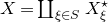 $X=\coprod _{\xi \in S} X_\xi ^\star$
is stratified as explained in Construction 2.21. The boundary of
$X=\coprod _{\xi \in S} X_\xi ^\star$
is stratified as explained in Construction 2.21. The boundary of $X$
is the union of the strata of codimension
$X$
is the union of the strata of codimension $\geqslant 1$
, and we denote by
$\geqslant 1$
, and we denote by $\mathcal{D} \!{\textit {iv}}^+_\flat$
the sheaf in the Zariski topology of effective Cartier divisors on
$\mathcal{D} \!{\textit {iv}}^+_\flat$
the sheaf in the Zariski topology of effective Cartier divisors on $X$
supported on the boundary.
$X$
supported on the boundary.
Let $\mathcal{C}$
be the cone sheaf on
$\mathcal{C}$
be the cone sheaf on $X$
. Assuming that
$X$
. Assuming that $Y$
is viable, we construct a homomorphism of sheaves of monoids on
$Y$
is viable, we construct a homomorphism of sheaves of monoids on $X$
:
$X$
:
 \begin{align*} \widetilde {D}\colon \mathcal{C} \to \mathcal{D} \!{\textit {iv}}^+_\flat, \end{align*}
which we call the divisor system.
For $\sigma \in T^{[0]}$
, denote by
$\sigma \in T^{[0]}$
, denote by $\varepsilon _\sigma \colon Y_\sigma \hookrightarrow Y$
the natural closed immersion, so that
$\varepsilon _\sigma \colon Y_\sigma \hookrightarrow Y$
the natural closed immersion, so that $\varepsilon =\textstyle \bigsqcup _{\sigma \in T^{[0]}}$ $\varepsilon _\sigma \colon X \to Y$
.
$\varepsilon _\sigma \colon X \to Y$
.
We use the notation set out in Construction 2.21.
Denote by $\widetilde {a} \colon S \to X$
the natural inclusion and by
$\widetilde {a} \colon S \to X$
the natural inclusion and by $\widetilde {b}\colon X \to S$
the retraction of Lemma 2.7: we have that
$\widetilde {b}\colon X \to S$
the retraction of Lemma 2.7: we have that $a(\eta , \sigma )=a(\eta ) \in Y_\sigma$
, and for
$a(\eta , \sigma )=a(\eta ) \in Y_\sigma$
, and for $x\in Y_\sigma$
,
$x\in Y_\sigma$
, $\widetilde {b} (x)=(b(x), \sigma )$
.
$\widetilde {b} (x)=(b(x), \sigma )$
.
More precisely, $\mathcal{C}$
is the sheaf on
$\mathcal{C}$
is the sheaf on $S$
of Construction 2.21 and we construct a sheaf homomorphism
$S$
of Construction 2.21 and we construct a sheaf homomorphism $\widetilde {b}^{-1} \mathcal{C} \to \mathcal{D} \!{\textit {iv}}^+_\flat$
, which is the same as a homomorphism
$\widetilde {b}^{-1} \mathcal{C} \to \mathcal{D} \!{\textit {iv}}^+_\flat$
, which is the same as a homomorphism $\mathcal{C} \to \widetilde {b}_\star \mathcal{D} \!{\textit {iv}}^+_\flat$
of sheaves on
$\mathcal{C} \to \widetilde {b}_\star \mathcal{D} \!{\textit {iv}}^+_\flat$
of sheaves on $S$
.
$S$
.
For all $\xi = (\eta , \sigma )\in S$
, let
$\xi = (\eta , \sigma )\in S$
, let
 \begin{align*} \widetilde {U}_\xi = \widetilde {b}^{-1} (S_{\geqslant \xi }) = \{x\in Y_\sigma \mid b(x)\geqslant \eta \}. \end{align*}
To construct our sheaf homomorphism, for all $\xi \in S$
we need to assign a monoid homomorphism:
$\xi \in S$
we need to assign a monoid homomorphism:
 \begin{align*} \widetilde {D}_\xi \colon C_\xi \to \operatorname {Div}^+_\flat (\widetilde {U}_\xi ) \end{align*}
and these monoid homomorphisms need to be compatible with generization in the obvious way.
In Definition 2.16, for $m\in C_\xi =\sigma \cap M_\eta$
we defined a Cartier divisor
$m\in C_\xi =\sigma \cap M_\eta$
we defined a Cartier divisor
 \begin{align*} D_{\eta ,\sigma } (m) \in \operatorname {Div}^+_\flat (\overline {U_\sigma } \cap U_\eta ) \end{align*}
Noting that $\widetilde {U}_\xi =\varepsilon _\sigma ^{-1}(\overline {U_\sigma } \cap U_\eta )$
, we define
$\widetilde {U}_\xi =\varepsilon _\sigma ^{-1}(\overline {U_\sigma } \cap U_\eta )$
, we define $\widetilde {D}_\xi (m)=\varepsilon _\sigma ^\star D_{\eta , \sigma } (m)$
.
$\widetilde {D}_\xi (m)=\varepsilon _\sigma ^\star D_{\eta , \sigma } (m)$
.
Definition 2.24. Let $Y$
be a viable ggtc space. The divisor system is the homomorphism of Zariski sheaves of monoids on
$Y$
be a viable ggtc space. The divisor system is the homomorphism of Zariski sheaves of monoids on $X=Y^{[0]}$
 \begin{align*} \widetilde {D} \colon \mathcal{C} \to \mathcal{D} \!{\textit {iv}}^+_\flat \quad \text{on}\; X \end{align*}
of Construction 2.23.
Remark 2.25. One can show that $\widetilde {D}$
is an isomorphism.
$\widetilde {D}$
is an isomorphism.
Notation 2.26. Let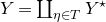 $Y=\coprod _{\eta \in T} Y^\star$
be a ggtc space,
$Y=\coprod _{\eta \in T} Y^\star$
be a ggtc space, $a\colon T\to Y$
the inclusion and
$a\colon T\to Y$
the inclusion and $b\colon Y \to T$
the retraction of Lemma 2.7. For all
$b\colon Y \to T$
the retraction of Lemma 2.7. For all $y\in Y$
, the open star of
$y\in Y$
, the open star of $y$
is
$y$
is
 \begin{align*} U_y=U_\eta ,\quad \text{where} \ y\in Y_\eta ^\star \end{align*}
and $U_\eta = b^{-1} T_{\geqslant \eta }$
is the open star of
$U_\eta = b^{-1} T_{\geqslant \eta }$
is the open star of $\eta$
, cf. Definition 2.8.
$\eta$
, cf. Definition 2.8.
Similarly let $\varepsilon \colon X=\coprod _{\xi \in S} X^\star _\xi \to Y$
be the normalization, stratified as in Construction 2.21,
$\varepsilon \colon X=\coprod _{\xi \in S} X^\star _\xi \to Y$
be the normalization, stratified as in Construction 2.21, $\widetilde {a}\colon S \to X$
the inclusion and
$\widetilde {a}\colon S \to X$
the inclusion and $\widetilde {b}\colon X\to S$
the retraction of Lemma 2.7. For all
$\widetilde {b}\colon X\to S$
the retraction of Lemma 2.7. For all $x\in X$
, the open star of
$x\in X$
, the open star of $x$
is
$x$
is
 \begin{align*} \widetilde {U}_x=\widetilde {U}_\xi ,\quad \text{where} \ x\in X_\xi ^\star \end{align*}
and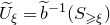 $\widetilde {U}_\xi = \widetilde {b}^{-1} (S_{\geqslant \xi })$
is the open star of
$\widetilde {U}_\xi = \widetilde {b}^{-1} (S_{\geqslant \xi })$
is the open star of $\xi$
, cf. Definition 2.8.
$\xi$
, cf. Definition 2.8.
Lemma 2.27.
Let $Y$
be a viable ggtc space,
$Y$
be a viable ggtc space, $\varepsilon \colon X \to Y$
the normalization stratified as in Construction 2.21
. For all
$\varepsilon \colon X \to Y$
the normalization stratified as in Construction 2.21
. For all $y\in Y$
, consider the fan
$y\in Y$
, consider the fan $\Sigma _y\subset M_y$
, and let
$\Sigma _y\subset M_y$
, and let $\sigma _1, \sigma _2\in \Sigma _y$
be two maximal cones adjacent along a submaximal cone
$\sigma _1, \sigma _2\in \Sigma _y$
be two maximal cones adjacent along a submaximal cone $\rho = \sigma _1 \cap \sigma _2$
. Then
$\rho = \sigma _1 \cap \sigma _2$
. Then $y\in Y_\rho$
and let
$y\in Y_\rho$
and let $x_1\in Y_{\sigma _1}\subset X$
,
$x_1\in Y_{\sigma _1}\subset X$
, $x_2 \in Y_{\sigma _2}\subset X$
be the two lifts, so
$x_2 \in Y_{\sigma _2}\subset X$
be the two lifts, so $C_{x_1}=\sigma _1$
,
$C_{x_1}=\sigma _1$
, $C_{x_2}=\sigma _2$
and in this sense
$C_{x_2}=\sigma _2$
and in this sense $C_{x_1}\cap C_{x_2}=\rho$
. There are obvious inclusions
$C_{x_1}\cap C_{x_2}=\rho$
. There are obvious inclusions
 \begin{align*} \iota _1\colon Y_\rho \hookrightarrow Y_{\sigma _1} \quad \textit{and}\quad \iota _2 \colon Y_{\rho }\hookrightarrow Y_{\sigma _2} \end{align*}
and we write (following Notation 2.26)
 \begin{align*} V_y=U_y\cap Y_\rho. \end{align*}
Note that $V_y=\iota _1^{-1}(\widetilde {U}_{x_1})=\iota _2^{-1}(\widetilde {U}_{x_2})$
.
$V_y=\iota _1^{-1}(\widetilde {U}_{x_1})=\iota _2^{-1}(\widetilde {U}_{x_2})$
.
In this situation, denote by $\iota _1^!\colon \operatorname {Div}^+_\flat \widetilde {U}_{x_1}\dashrightarrow \operatorname {Div}^+_\flat V_y$
the partially defined restriction homomorphism that is defined for each divisor that intersects
$\iota _1^!\colon \operatorname {Div}^+_\flat \widetilde {U}_{x_1}\dashrightarrow \operatorname {Div}^+_\flat V_y$
the partially defined restriction homomorphism that is defined for each divisor that intersects $V_y$
properly, and similarly
$V_y$
properly, and similarly $\iota _2^!$
.
$\iota _2^!$
.
The following diagram is commutative.
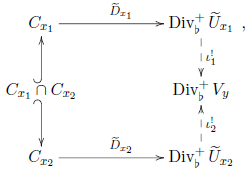
Here we note that the restriction $\iota _1^!$
is well-defined on
$\iota _1^!$
is well-defined on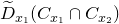 $\widetilde {D}_{x_1}(C_{x_1}\cap C_{x_2})$
and, similarly,
$\widetilde {D}_{x_1}(C_{x_1}\cap C_{x_2})$
and, similarly, $\iota _2^!$
is well-defined on
$\iota _2^!$
is well-defined on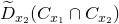 $\widetilde {D}_{x_2} (C_{x_1}\cap C_{x_2})$
).
$\widetilde {D}_{x_2} (C_{x_1}\cap C_{x_2})$
).
The diagram is compatible with generization in the obvious way.
Proof. Straightforward.
3. Construction of the sheaf
$\mathcal{LS}_Y$

In this section, given a viable ggtc space $Y$
, we construct a sheaf of sets
$Y$
, we construct a sheaf of sets $\mathcal{L}\mathcal{S}_Y$
on
$\mathcal{L}\mathcal{S}_Y$
on $Y$
, intrinsic to
$Y$
, intrinsic to $Y$
. In Section 4, we prove that
$Y$
. In Section 4, we prove that $\mathcal{LS}_Y$
classifies compatible log structures on
$\mathcal{LS}_Y$
classifies compatible log structures on $Y$
over
$Y$
over $k^\dagger$
. We refer to Section 1.1 for an informal summary of the construction of
$k^\dagger$
. We refer to Section 1.1 for an informal summary of the construction of $\mathcal{LS}_Y$
.
$\mathcal{LS}_Y$
.
In Section 3.1, for every slab $\rho \in T^{[1]}$
, we give the construction of the slab line bundle
$\rho \in T^{[1]}$
, we give the construction of the slab line bundle $\mathcal{L}_\rho$
on
$\mathcal{L}_\rho$
on $Y_\rho$
. In Corollary 3.7 of Section 3.2, we show that, for every joint
$Y_\rho$
. In Corollary 3.7 of Section 3.2, we show that, for every joint $\omega \in T^{[2]}$
, the restrictions
$\omega \in T^{[2]}$
, the restrictions $\mathcal{L}_{\rho |Y_\omega }$
for all
$\mathcal{L}_{\rho |Y_\omega }$
for all $\omega \lt \rho$
satisfy the joint condition. This is seen as an easy consequence of an abstract joint condition that is stated in Lemma 3.6. In Definition 3.9, the joint conditions are used to define the sheaf
$\omega \lt \rho$
satisfy the joint condition. This is seen as an easy consequence of an abstract joint condition that is stated in Lemma 3.6. In Definition 3.9, the joint conditions are used to define the sheaf $\mathcal{LS}_Y$
.
$\mathcal{LS}_Y$
.
The construction of the slab line bundles $\mathcal{L}_\rho$
and, in particular, the formulation of the joint condition, are delicate. In order to glue the slab bundles from local data, and in order to formulate the joint condition, we need carefully to keep track of isomorphisms between line bundles and not just the line bundles themselves. For this reason it is necessary that we work with the Picard
$\mathcal{L}_\rho$
and, in particular, the formulation of the joint condition, are delicate. In order to glue the slab bundles from local data, and in order to formulate the joint condition, we need carefully to keep track of isomorphisms between line bundles and not just the line bundles themselves. For this reason it is necessary that we work with the Picard $2$
-group
$2$
-group $\operatorname {\underline {Pic}} Y$
(and, implicitly, the Picard stack
$\operatorname {\underline {Pic}} Y$
(and, implicitly, the Picard stack ${\underline {\mathcal{P} ic}}_Y$
), for which we refer the reader to [Reference Deligne, Artin, Grothendieck and VerdierDel73, Section 1.4].
${\underline {\mathcal{P} ic}}_Y$
), for which we refer the reader to [Reference Deligne, Artin, Grothendieck and VerdierDel73, Section 1.4].
3.1 The slab line bundles
In this subsection we fix throughout a viable ggtc space $Y$
. The goal is to construct, for all
$Y$
. The goal is to construct, for all $\rho \in T^{[1]}$
, a line bundle
$\rho \in T^{[1]}$
, a line bundle $\mathcal{L}_\rho \in \operatorname {\underline {Pic}} Y_\rho$
that we call a slab bundle.
$\mathcal{L}_\rho \in \operatorname {\underline {Pic}} Y_\rho$
that we call a slab bundle.
Before describing the construction, we recall the following.
Definition 3.1. Let $M$
be an abelian group and
$M$
be an abelian group and $(\underline {A},\otimes ,{\bf 1})$
a strictly commutative
$(\underline {A},\otimes ,{\bf 1})$
a strictly commutative $2$
-group, where:
$2$
-group, where:
-
(a) for objects
$A_1$
,
$A_2$
of
$\underline {A}$
, we denote bythe isomorphism provided by the
\begin{align*} t\colon A_1\otimes A_2 \overset {\cong }{\longrightarrow } A_2\otimes A_1 \end{align*}
$2$
-group structure;
-
(b) for objects
$A_1$
,
$A_2$
,
$A_3$
of
$\underline {A}$
, we denote bythe isomorphism provided by the
\begin{align*} s\colon A_1\otimes (A_2\otimes A_3) \overset {\cong }{\longrightarrow } (A_1\otimes A_2) \otimes A_3 \end{align*}
$2$
-group structure.


A $2$
-homomorphism
$2$
-homomorphism $\mu \colon M \to \underline {A}$
is an assignment
$\mu \colon M \to \underline {A}$
is an assignment $\mu \colon M \to \operatorname {Ob} \underline {A}$
together with the datum, for all
$\mu \colon M \to \operatorname {Ob} \underline {A}$
together with the datum, for all $m_1,m_2\in M$
, of an isomorphism
$m_1,m_2\in M$
, of an isomorphism
 \begin{align*} \mu (m_1+m_2)\overset {\cong }{\longrightarrow } \mu (m_1)\otimes \mu (m_2) \end{align*}
such that:
-
(i)
$\mu (0)={\bf 1}$
; -
(ii) for all
$m_1,m_2\in M$
the following diagrams are commutative -
(iii) for all
$m_1,m_2,m_3\in M$
the following diagrams are commutative


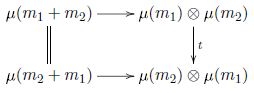


Lemma 3.2.
Let $Y$
be a viable ggtc space and
$Y$
be a viable ggtc space and $\rho \in T^{[1]}$
a slab. Fix
$\rho \in T^{[1]}$
a slab. Fix $y\in Y_\rho$
, and use the notation of Lemma 2.27: in particular, denote by
$y\in Y_\rho$
, and use the notation of Lemma 2.27: in particular, denote by $\sigma _1,\sigma _2$
the maximal cones of
$\sigma _1,\sigma _2$
the maximal cones of $\Sigma _y \subset M_y$
that meet along
$\Sigma _y \subset M_y$
that meet along $\rho$
. Denote by
$\rho$
. Denote by
 \begin{align*} \mu _i\colon M_y \to \operatorname {\underline {Pic}} (V_y) \end{align*}
the unique $2$
-homomorphism such that, for
$2$
-homomorphism such that, for $m\in C_{x_i}\subset M_y$
,
$m\in C_{x_i}\subset M_y$
, $\mu _i(m)=\iota _i^\star \bigl (\mathcal{O}_{\widetilde {U}_{x_i}}\bigl (\widetilde {D}_{x_i}(m)\bigr )\bigr )$
. Note that
$\mu _i(m)=\iota _i^\star \bigl (\mathcal{O}_{\widetilde {U}_{x_i}}\bigl (\widetilde {D}_{x_i}(m)\bigr )\bigr )$
. Note that $\mu _1=\mu _2$
on the subspace
$\mu _1=\mu _2$
on the subspace $\langle C_{x_1}\cap C_{x_2} \rangle =\langle \rho \rangle$
and denote this restricted
$\langle C_{x_1}\cap C_{x_2} \rangle =\langle \rho \rangle$
and denote this restricted $2$
-homomorphism simply by
$2$
-homomorphism simply by $\mu$
.
$\mu$
.
Let $d \in \sigma _2^\vee \subset \operatorname {Hom} (M_y, \mathbb{Z})$
be the unique primitive vector that pairs to zero with all points in
$d \in \sigma _2^\vee \subset \operatorname {Hom} (M_y, \mathbb{Z})$
be the unique primitive vector that pairs to zero with all points in $\rho$
. Next choose
$\rho$
. Next choose $v \in M_y$
such that
$v \in M_y$
such that $\langle d, v\rangle=1$
. We define a line bundle
$\langle d, v\rangle=1$
. We define a line bundle $\lambda (v)$
on
$\lambda (v)$
on $V_y$
as
$V_y$
as
 \begin{align*} \lambda (v)=\mu _1(-v)\otimes \mu _2(v). \end{align*}
Then we have the following.
-
(1) The line bundle
$\lambda (v)$
is independent on the choice of
$v$
in the following sense: for all
$r\in \langle \rho \rangle$
, we construct an isomorphism
\begin{align*} \psi _r\colon \lambda (v)\overset {\cong }{\longrightarrow }\lambda (r+v). \end{align*}
-
(2) The set of these isomorphisms has the cocycle property:
-
(i) for all
$v \in \sigma _2$
such that
$\langle d, v\rangle=1$
,
$\psi _{0}=\operatorname {id}_{\lambda (v)}$
; -
(ii) for all
$v \in \sigma _2$
such that
$\langle d, v\rangle=1$
, and for all
$r,s\in \langle \rho \rangle$
, the following diagram is commutative.
-
-
(3) Similarly,
$\lambda (v)$
does not depend on the choice of numbering of
$\sigma _1$
,
$\sigma _2$
in the sense that if we swap numbering, then
$d$
is changed into
$-d$
,
$v$
into
$-v$
, and the line bundle into
$\mu _2(v)\otimes \mu _1(-v)$
.


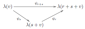



Proof.
In the diagram in Figure 1, the outer pentagon is commutative by the pentagon axiom and the internal part of the diagram gives the construction of $\psi _r\colon \lambda (v)\to \lambda (r+v)$
. (Note that, since
$\psi _r\colon \lambda (v)\to \lambda (r+v)$
. (Note that, since $r\in \langle \rho \rangle$
,
$r\in \langle \rho \rangle$
, $\mu _1(r)=\mu _2(r)$
, and we write simply
$\mu _1(r)=\mu _2(r)$
, and we write simply $\mu (r)$
to signify either of these two equal line bundles.)
$\mu (r)$
to signify either of these two equal line bundles.)
Construction of $\psi_r: \lambda (v) \rightarrow \lambda(r+v) $
.
$\psi_r: \lambda (v) \rightarrow \lambda(r+v) $
.
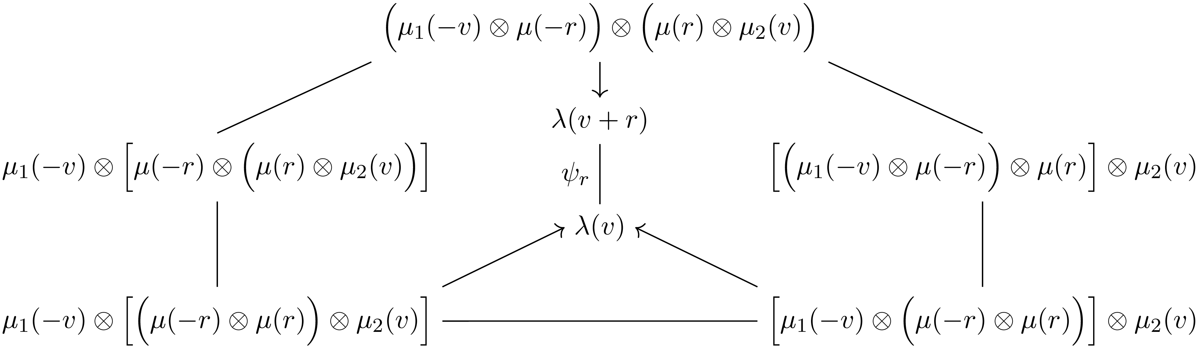
Figure 1. Long description
The equation illustrates a complex mathematical relationship involving tensor products and functions. It begins with a tensor product of two terms, each involving functions and variables. The equation then progresses through several transformations, including the application of functions and tensor products, leading to a final simplified form. The structure involves multiple levels of nested tensor products and functions, demonstrating a detailed and intricate mathematical process.
The statement that for all $r,s\in \langle \rho \rangle$
,
$r,s\in \langle \rho \rangle$
, $\psi _{r+s}=\psi _r\circ \psi _s$
follows from contemplating the diagram in Figure 2, where the outer circle is commutative by MacLane coherence theorem for monoidal categories. For reasons of space we are suppressing the
$\psi _{r+s}=\psi _r\circ \psi _s$
follows from contemplating the diagram in Figure 2, where the outer circle is commutative by MacLane coherence theorem for monoidal categories. For reasons of space we are suppressing the $\otimes$
symbols.
$\otimes$
symbols.
Construction 3.3. For every slab $\rho \in T^{[1]}$
, we construct a line bundle
$\rho \in T^{[1]}$
, we construct a line bundle $\mathcal{L}_\rho$
on
$\mathcal{L}_\rho$
on $Y_\rho$
, which we will call a slab bundle.
$Y_\rho$
, which we will call a slab bundle.
Proof that $\psi_{r+s}=\psi_r \circ \psi_s$
.
$\psi_{r+s}=\psi_r \circ \psi_s$
.
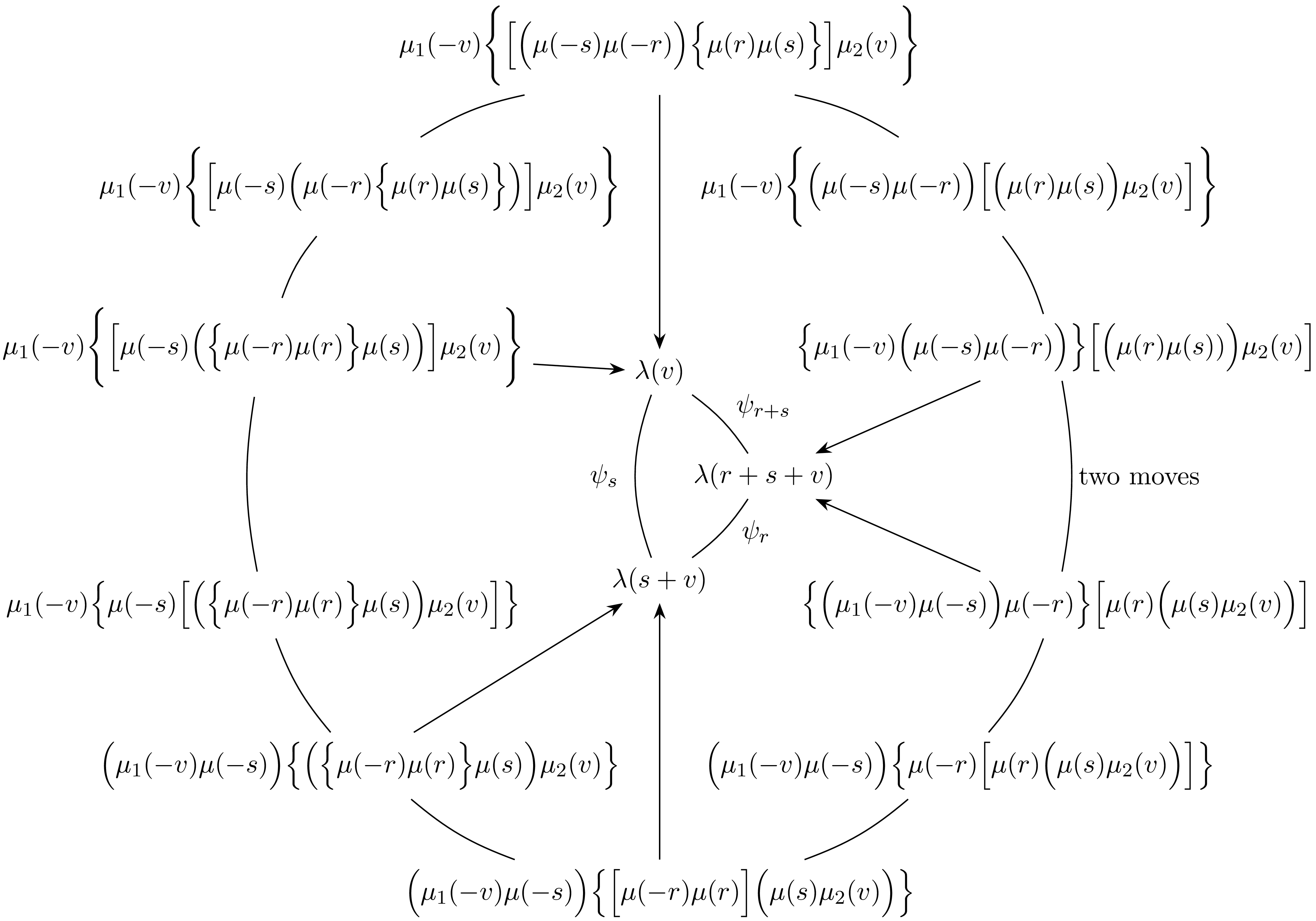
Figure 2. Long description
The equation features a series of terms involving variables mu, lambda, and psi, with various exponents and groupings. It includes terms such as mu1 negative v, mu negative s, mu negative r, and mu2 v, arranged in a complex structure with nested parentheses and arrows indicating transformations or relationships between terms.
Fix throughout $\rho \in T^{[1]}$
.
$\rho \in T^{[1]}$
.
First, we construct a covering of $Y_\rho$
by Zariski open subsets. Note that
$Y_\rho$
by Zariski open subsets. Note that
 \begin{align*} Y_\rho = \coprod _{\{\tau \in T\mid \tau \leqslant \rho \}} Y_\tau ^\star \end{align*}
is itself a stratified space. We denote by $T_\rho = \{\tau \in T\mid \tau \leqslant \rho \}$
the index poset for the strata of
$T_\rho = \{\tau \in T\mid \tau \leqslant \rho \}$
the index poset for the strata of $Y_\rho$
. For all
$Y_\rho$
. For all $\tau \in T_\rho$
, we denote by
$\tau \in T_\rho$
, we denote by $V_\tau \subset Y_\rho$
the open star of
$V_\tau \subset Y_\rho$
the open star of $\tau$
in
$\tau$
in $Y_\rho$
. It is clear that
$Y_\rho$
. It is clear that $\{V_\tau \mid \tau \in T_\rho \}$
is a Zariski open cover of
$\{V_\tau \mid \tau \in T_\rho \}$
is a Zariski open cover of $Y_\rho$
.
$Y_\rho$
.
Now choose a global numbering for the maximal cones incident at $\rho$
: in other words, for all
$\rho$
: in other words, for all $\tau \in T_\rho$
, a numbering
$\tau \in T_\rho$
, a numbering $\sigma _1(\tau )$
,
$\sigma _1(\tau )$
, $\sigma _2(\tau )$
of the two maximal cones in
$\sigma _2(\tau )$
of the two maximal cones in $\Sigma _\tau$
incident at
$\Sigma _\tau$
incident at $\rho$
,Footnote
14
satisfying the consistency condition. If
$\rho$
,Footnote
14
satisfying the consistency condition. If $\tau _1\leqslant \tau _2$
, then, for
$\tau _1\leqslant \tau _2$
, then, for $i=1,2$
,
$i=1,2$
, $\sigma _i(\tau _1)$
maps to
$\sigma _i(\tau _1)$
maps to $\sigma _i(\tau _2)$
under the natural projection
$\sigma _i(\tau _2)$
under the natural projection $M_{\tau _1} \to M_{\tau _2}=M_{\tau _1}/\langle \tau _2\rangle$
.Footnote
15
Note that there are precisely two global numberings.
$M_{\tau _1} \to M_{\tau _2}=M_{\tau _1}/\langle \tau _2\rangle$
.Footnote
15
Note that there are precisely two global numberings.
For all $\tau$
, Let
$\tau$
, Let $d_\tau \in \sigma _2(\tau )^\vee \subset \operatorname {Hom} (M_\tau , \mathbb{Z})$
be the unique primitive vector that pairs to zero with all points in
$d_\tau \in \sigma _2(\tau )^\vee \subset \operatorname {Hom} (M_\tau , \mathbb{Z})$
be the unique primitive vector that pairs to zero with all points in $\rho$
. Next choose
$\rho$
. Next choose $v_\tau \in M_\tau$
such that
$v_\tau \in M_\tau$
such that $\langle d_\tau , v_\tau \rangle=1$
. Following Lemma 3.2 with
$\langle d_\tau , v_\tau \rangle=1$
. Following Lemma 3.2 with $y=\tau$
, we define a line bundle
$y=\tau$
, we define a line bundle $\lambda (v_\tau )$
on
$\lambda (v_\tau )$
on $V_\tau$
as
$V_\tau$
as
 \begin{align*} \lambda (v_\tau )=\mu _1(\tau ) (-v_\tau )\otimes \mu _2(\tau ) (v_\tau ) \end{align*}
where we denote by $\mu _i(\tau ) \colon M_{\tau } \to \operatorname {\underline {Pic}} (V_\tau )$
the
$\mu _i(\tau ) \colon M_{\tau } \to \operatorname {\underline {Pic}} (V_\tau )$
the $2$
-homomorphisms of Lemma 3.2.
$2$
-homomorphisms of Lemma 3.2.
Next we glue the $\lambda (v_\tau )$
to a line bundle on all of
$\lambda (v_\tau )$
to a line bundle on all of $Y_\rho$
. If
$Y_\rho$
. If $\tau _1\leqslant \tau _2$
, then:
$\tau _1\leqslant \tau _2$
, then:
-
(1)
$V_{\tau _2}\subset V_{\tau _1}$
; -
(2) we have an identification
$\pi =\pi _{\tau _1,\tau _2}\colon M_{\tau _1} \to M_{\tau _1}/\langle \tau _2\rangle =M_{\tau _2}$
; -
(3) under the dual injection
$N_{\tau _2}\subset N_{\tau _1}$
,
$d_{\tau _2}$
is identified with
$d_{\tau _1}$
and
$\langle d_{\tau _2,}\pi (v_{\tau _1}) \rangle=1$
and hence we can form
$r_{\tau _1,\tau _2}= \pi (v_{\tau _1})-v_{\tau _2}\in \langle \rho \rangle \cap M_{\tau _2}$
.






At this point, we
 \begin{align*} \text{glue $\lambda(v_{\tau_1})_{|V_{\tau_2}}=\lambda(v_{\pi(v_{\tau_1})})$ to $\lambda(v_{\tau_2})$ with $\psi _{r(\tau_1,\tau_2)} \colon \lambda(v_{\pi(v_{\tau_1})})\overset {\cong }{\longrightarrow } \lambda(v_{\tau_2})$} \end{align*}
whose construction is given by Lemma 3.2.
Next, we keep gluing on all the line bundles on all the $V_\tau$
formed from both choices of numbering and all system of vectors
$V_\tau$
formed from both choices of numbering and all system of vectors $(v_{\tau })_{\tau \in M_\tau }$
as above by using the
$(v_{\tau })_{\tau \in M_\tau }$
as above by using the $\psi$
isomorphisms as above. The cocycle condition ensures that all these gluings can be done consistently.
$\psi$
isomorphisms as above. The cocycle condition ensures that all these gluings can be done consistently.
We denote by $\mathcal{L}_\rho$
the resulting line bundle on
$\mathcal{L}_\rho$
the resulting line bundle on $Y_\rho$
.
$Y_\rho$
.
Definition 3.4. Let $Y=\coprod _{\tau \in T} Y^\star _\tau$
be a viable ggtc space and
$Y=\coprod _{\tau \in T} Y^\star _\tau$
be a viable ggtc space and $\rho \in T^{[1]}$
. We call the line bundle
$\rho \in T^{[1]}$
. We call the line bundle $\mathcal{L}_\rho$
on
$\mathcal{L}_\rho$
on $Y_\rho$
of Construction 3.3 the slab bundle.
$Y_\rho$
of Construction 3.3 the slab bundle.
Abusing notation, we also denote by $\mathcal{L}_\rho$
the direct image of this line bundle under the inclusion
$\mathcal{L}_\rho$
the direct image of this line bundle under the inclusion $Y_\rho \hookrightarrow Y$
.
$Y_\rho \hookrightarrow Y$
.
3.2 The joint condition and the sheaf
$\mathcal{LS}_Y$

We show that for every joint $\omega \in T^{[2]}$
the restrictions of all
$\omega \in T^{[2]}$
the restrictions of all $\mathcal{L}_\rho$
with
$\mathcal{L}_\rho$
with $\omega \lt \rho$
to
$\omega \lt \rho$
to $Y_\omega$
satisfy a relation. We then use this relation to define a subsheaf
$Y_\omega$
satisfy a relation. We then use this relation to define a subsheaf $\mathcal{LS}_Y \subset \bigoplus _{\rho \in T^{[1]}} \mathcal{L}_\rho$
. A similar relation first appeared as a relation of elements in a local computation in Theorem 3.22 in [Reference Gross and SiebertGS06].
$\mathcal{LS}_Y \subset \bigoplus _{\rho \in T^{[1]}} \mathcal{L}_\rho$
. A similar relation first appeared as a relation of elements in a local computation in Theorem 3.22 in [Reference Gross and SiebertGS06].
The following definition and theorem are stated in terms of a strictly commutative $2$
-group
$2$
-group $\underline {A}$
, because this is what we need. The statement contains as a special case the situation where
$\underline {A}$
, because this is what we need. The statement contains as a special case the situation where $\underline {A}$
is the categorification of an abelian group
$\underline {A}$
is the categorification of an abelian group $A$
, where a more concrete formulation of the definition and theorem are possible.
$A$
, where a more concrete formulation of the definition and theorem are possible.
Definition 3.5. Let $M$
be a finitely generated free abelian group and
$M$
be a finitely generated free abelian group and $\Sigma$
a complete fan in
$\Sigma$
a complete fan in $M$
. Let
$M$
. Let $\underline {A}$
be a strictly commutative
$\underline {A}$
be a strictly commutative $2$
-group. A continuous piecewise linear
$2$
-group. A continuous piecewise linear $2$
-homomorphism
$2$
-homomorphism $\mu \colon M\to \underline {A}$
with respect to
$\mu \colon M\to \underline {A}$
with respect to $\Sigma$
is a collection of
$\Sigma$
is a collection of $2$
-homomorphisms
$2$
-homomorphisms
 \begin{align*} \mu _\sigma \colon M \to \underline {A}\, , \end{align*}
one for each maximal cone $\sigma \in \Sigma$
, with the property that whenever two maximal cones
$\sigma \in \Sigma$
, with the property that whenever two maximal cones $\sigma _1,\sigma _2$
share a submaximal cone
$\sigma _1,\sigma _2$
share a submaximal cone $\rho =\sigma _1\cap \sigma _2$
then the restrictions of
$\rho =\sigma _1\cap \sigma _2$
then the restrictions of $\mu _{\sigma _1}, \mu _{\sigma _2}$
to
$\mu _{\sigma _1}, \mu _{\sigma _2}$
to $\langle \rho \rangle$
are equal.
$\langle \rho \rangle$
are equal.
Lemma 3.6 (Abstract joint condition lemma). Let $M$
be a lattice,
$M$
be a lattice, $N=\operatorname {Hom} (M,\mathbb{Z})$
, and assume given a surjective homomorphism
$N=\operatorname {Hom} (M,\mathbb{Z})$
, and assume given a surjective homomorphism $\pi \colon M \to \overline {M}$
, where
$\pi \colon M \to \overline {M}$
, where $\overline {M}$
is a rank two lattice endowed with a complete fan
$\overline {M}$
is a rank two lattice endowed with a complete fan $\overline {\Sigma }$
. Endow
$\overline {\Sigma }$
. Endow $M$
with the fan
$M$
with the fan
 \begin{align*} \Sigma = \{\pi ^{-1}(\eta )\mid \eta \in \overline {\Sigma }\} \end{align*}
We denote the cones of $\Sigma$
as follows:
$\Sigma$
as follows:
-
– the codimension-
$2$
subspace (also known as a joint)
$\omega =\pi ^{-1}\{0\}$
; -
– cyclically ordered codimension-
$1$
cones (also known as slabs)
$\rho _1, \ldots , \rho _n$
incident at
$\omega$
; -
– maximal cones
$\sigma _i=\langle \rho _i\cup \rho _{i+1}\rangle _+$
(for
$i=1,\ldots , n$
with the convention that
$\rho _{n+1}=\rho _1$
).





Let $(\underline {A},+,0_{\underline {A}})$
be a strictly commutative
$(\underline {A},+,0_{\underline {A}})$
be a strictly commutative $2$
-group and
$2$
-group and $\mu \colon M \to \underline {A}$
a continuous piecewise linear
$\mu \colon M \to \underline {A}$
a continuous piecewise linear $2$
-homomorphism with respect to
$2$
-homomorphism with respect to $\Sigma$
. Denote by
$\Sigma$
. Denote by $\mu _i=\mu _{\sigma _i}$
the
$\mu _i=\mu _{\sigma _i}$
the $2$
-homomorphism for
$2$
-homomorphism for $\sigma _i$
that forms part of the datum
$\sigma _i$
that forms part of the datum $\mu$
. Let
$\mu$
. Let $d_1, \ldots , d_n \in N$
be the primitive normals to the slabs
$d_1, \ldots , d_n \in N$
be the primitive normals to the slabs $\rho _1, \ldots ,\rho _n$
, such that
$\rho _1, \ldots ,\rho _n$
, such that $d_i\ge 0$
on
$d_i\ge 0$
on $\rho _{i+1}$
.
$\rho _{i+1}$
.
Choose $v_i\in M$
such that
$v_i\in M$
such that $\langle d_i,v_i\rangle=1$
and define
$\langle d_i,v_i\rangle=1$
and define
 \begin{align} \lambda (v_i)=\mu _{i-1}(-v_i)+\mu _i(v_i). \end{align}
-
(1) We construct the joint isomorphism
(3.2)
\begin{align} \sum _{i=1}^n d_i\otimes \lambda (v_i) \overset {\cong }{\longrightarrow } 0 \otimes 0_{\underline {A}} \;\; \text{in}\;\;N\otimes \underline {A} =\underline {\operatorname {2-Hom}} (M,\underline {A}), \end{align}
-
(2) The isomorphism constructed in part (1) does not depend on the choice of
$v_i$
in the following sense. For all
$i=1,\ldots ,n$
and
$r_i\in \langle \rho _i \rangle$
we construct isomorphisms
such that the following diagram is commutative
\begin{align*} \psi _{r_i} \colon \lambda (v_i) \overset {\cong }{\longrightarrow } \lambda (v_i+r_i) \end{align*}
and, furthermore, the set of these isomorphisms has the cocycle property:
-
(i)
$\psi _{0}=\operatorname {id}$
; -
(ii) for all
$r_i,s_i\in \langle \rho _i\rangle$
,
$\psi _{r_i+s_i}=\psi _{r_i}\circ \psi _{s_i}$
.
-
-
(3) The joint isomorphism does not depend on the cyclic ordering in the sense that the isomorphism from the opposite ordering relates to the given one by a global multiplication by
$(-1)$
.


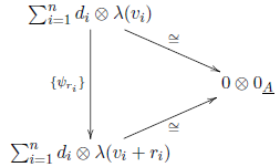




Proof.
For all $w\in M$
we produce an isomorphism
$w\in M$
we produce an isomorphism $\sum _{i=1}^n d_i(w)\lambda (v_i) \cong 0_{\underline {A}}$
in
$\sum _{i=1}^n d_i(w)\lambda (v_i) \cong 0_{\underline {A}}$
in $\underline {A}$
. The key observation is that for all
$\underline {A}$
. The key observation is that for all $i$
$i$
 \begin{align*} d_i\left (-d_i(w) v_i +w \right ) = -d_i(w)\underbrace {d_i(v_i)}_{=1}+d_i(w)=0. \end{align*}
Hence, $-d_i(w) v_i +w \in \langle \rho _i\rangle$
and therefore
$-d_i(w) v_i +w \in \langle \rho _i\rangle$
and therefore $\mu _{i-1}\bigl (-d_{i}(w)v_i+w\bigr )=\mu _i\bigl (-d_i(w)v_i+w\bigr )$
. Rewriting and using the natural transformations of functors provided by the monoidal structure of
$\mu _{i-1}\bigl (-d_{i}(w)v_i+w\bigr )=\mu _i\bigl (-d_i(w)v_i+w\bigr )$
. Rewriting and using the natural transformations of functors provided by the monoidal structure of $\underline {A}$
yields
$\underline {A}$
yields
 \begin{align} d_i(w)\mu _{i-1}(-v_i) \cong d_i(w)\mu _i(-v_i) + \mu _i(w) -\mu _{i-1}(w). \end{align}
The sum (3.2) in the assertion can be identified as a telescoping sum when writing
 \begin{align*} \begin{split} \sum _{i=1}^n d_i(w) \lambda (v_i) \stackrel {(3.1)}{\cong } & \hspace {.5cm}d_1(w) \bigl (\mu _n(-v_1)+\mu _1(v_1)\bigr )\\[-3mm] & +d_2(w)\bigl (\mu _1(-v_2)+\mu _2(v_2) \bigr )\\ & +d_3(w) \bigl (\mu _2(-v_3)+\mu _3(v_3) \bigr )\\ & \hspace {.5cm}\vdots \\ \stackrel {(3.3)}{\cong } & \hspace {.5cm}d_1(w)\bigl (\mu _1(-v_1)+\mu _1(v_1)\bigr )+\mu _1(w)-\mu _n(w) \\ & +d_2(w)\bigl ( \mu _2(-v_2)+\mu _2(v_2)\bigr )+\mu _2(w)-\mu _1(w)\\ & +d_3(w)\bigl ( \mu _3(-v_3)+\mu _3(v_3)\bigr )+\mu _3(w)-\mu _2(w)\\ & \hspace {.5cm}\vdots \\ \cong & \hspace {.5cm} 0_{\underline {A}}. \end{split} \end{align*}
The resulting isomorphism to $0_{\underline {A}}$
does not depend on choices, that is, the order of association and commutation in
$0_{\underline {A}}$
does not depend on choices, that is, the order of association and commutation in $\underline {A}$
, by the MacLane coherence theorem for
$\underline {A}$
, by the MacLane coherence theorem for $2$
-groups.
$2$
-groups.
For the independence on the choice of $v_i$
, part (1) is proved in the same way as the corresponding statement in Lemma 3.2. The proof of part (2) is straightforward and we omit the details.
$v_i$
, part (1) is proved in the same way as the corresponding statement in Lemma 3.2. The proof of part (2) is straightforward and we omit the details.
Corollary 3.7.
Let $Y$
be a viable ggtc space,
$Y$
be a viable ggtc space, $\omega \in T^{[2]}$
a joint, and
$\omega \in T^{[2]}$
a joint, and $\rho _1, \ldots , \rho _n$
a cyclical ordering of the slabs incident at
$\rho _1, \ldots , \rho _n$
a cyclical ordering of the slabs incident at $\omega$
. Let
$\omega$
. Let $d_1, \ldots , d_n \in N_\omega$
be the primitive normals to the slabs
$d_1, \ldots , d_n \in N_\omega$
be the primitive normals to the slabs $\rho _1, \ldots ,\rho _n$
, such that
$\rho _1, \ldots ,\rho _n$
, such that $d_i\ge 0$
on
$d_i\ge 0$
on $\rho _{i+1}$
.
$\rho _{i+1}$
.
We construct a joint isomorphism:
 \begin{align} J_\omega \colon \bigotimes _{i=1}^n d_i\otimes \mathcal{L}_{\rho _i|Y_\omega } \cong 0 \otimes \mathcal{O}_{Y_\omega } \quad \text{in} \ N_\omega \otimes \operatorname {\underline {Pic}} Y_\omega. \end{align}
Sketch of proof.
Fix throughout a joint $\omega \in T^{[2]}$
.
$\omega \in T^{[2]}$
.
The space $Y_\omega =\coprod _{\{\tau \in T \mid \tau \leqslant \omega \}} Y_\tau ^\star$
is stratified. We denote by
$Y_\omega =\coprod _{\{\tau \in T \mid \tau \leqslant \omega \}} Y_\tau ^\star$
is stratified. We denote by $T_\omega =\{\tau \in T \mid \tau \leqslant \omega \}$
the index poset for the strata of
$T_\omega =\{\tau \in T \mid \tau \leqslant \omega \}$
the index poset for the strata of $Y_\omega$
. For all
$Y_\omega$
. For all $\tau \in T_\omega$
, we denote by
$\tau \in T_\omega$
, we denote by $U_\tau \subset Y$
the open star of
$U_\tau \subset Y$
the open star of $\tau$
in
$\tau$
in $Y$
. It is clear that
$Y$
. It is clear that $\{U_\tau \cap Y_\omega \mid \tau \leqslant \omega \}$
is a Zariski open cover of
$\{U_\tau \cap Y_\omega \mid \tau \leqslant \omega \}$
is a Zariski open cover of $Y_\omega$
.
$Y_\omega$
.
Now $\Sigma _\omega$
is a fan in a rank two lattice
$\Sigma _\omega$
is a fan in a rank two lattice $M_\omega$
. Denote the cones of
$M_\omega$
. Denote the cones of $\Sigma _\omega$
as follows:
$\Sigma _\omega$
as follows:
-
– the cone
$(0)$
, corresponding to the joint
$\omega$
itself; -
– cyclically ordered rays
$\overline {\rho }_1,\ldots , \overline {\rho }_n$
, also know as slabs; -
– maximal cones
$\overline {\sigma }_i=\langle \overline {\rho }_i,\overline {\rho }_{i+1}\rangle _+$
.



Denote by $d_1,\ldots , d_n\in N_\omega$
the primitive normals to the slabs
$d_1,\ldots , d_n\in N_\omega$
the primitive normals to the slabs $\overline {\rho }_1, \ldots , \overline {\rho }_n$
such that
$\overline {\rho }_1, \ldots , \overline {\rho }_n$
such that $d_i\gt 0$
on
$d_i\gt 0$
on $\overline {\rho }_{i+1}$
.
$\overline {\rho }_{i+1}$
.
For all $i$
, Construction 3.3 constructs a slab bundle
$i$
, Construction 3.3 constructs a slab bundle $\mathcal{L}_{\rho _i}$
on
$\mathcal{L}_{\rho _i}$
on $Y_{\rho _i}$
.
$Y_{\rho _i}$
.
The bundles $\mathcal{L}_{\rho _i}$
are obtained from gluing together certain bundles constructed on certain open covers of
$\mathcal{L}_{\rho _i}$
are obtained from gluing together certain bundles constructed on certain open covers of $Y_{\rho _i}$
. We are only interested in the open subsets
$Y_{\rho _i}$
. We are only interested in the open subsets $U_\tau \cap Y_{\rho _i}$
for
$U_\tau \cap Y_{\rho _i}$
for $\tau \in T_\omega$
: these open subsets do not cover all of
$\tau \in T_\omega$
: these open subsets do not cover all of $Y_{\rho _i}$
but they do cover all of
$Y_{\rho _i}$
but they do cover all of $Y_\omega$
and, hence, they are sufficient for working with
$Y_\omega$
and, hence, they are sufficient for working with $\mathcal{L}_{\rho _i|Y_\omega }$
. Let us fix
$\mathcal{L}_{\rho _i|Y_\omega }$
. Let us fix $\tau \in T_\omega$
and focus on one of these open subsets
$\tau \in T_\omega$
and focus on one of these open subsets $U_\tau$
.
$U_\tau$
.
We are going to apply Lemma 3.6 to the situation $M=M_\tau$
,
$M=M_\tau$
, $\overline {M}=M_\omega =M/\langle \omega \rangle$
,
$\overline {M}=M_\omega =M/\langle \omega \rangle$
, $\pi \colon M \to \overline {M}$
the projection to the quotient,
$\pi \colon M \to \overline {M}$
the projection to the quotient, $\overline {\Sigma }=\Sigma _\omega$
, and
$\overline {\Sigma }=\Sigma _\omega$
, and $\Sigma =\omega ^{-1} \Sigma _\tau$
the localized fan. Abusing notation slightly, we denote by
$\Sigma =\omega ^{-1} \Sigma _\tau$
the localized fan. Abusing notation slightly, we denote by $\omega =\pi ^{-1}(0)$
,
$\omega =\pi ^{-1}(0)$
, $\rho _i=\pi ^{-1}(\overline {\rho }_i)$
,
$\rho _i=\pi ^{-1}(\overline {\rho }_i)$
, $\sigma _i=\pi ^{-1}(\overline {\sigma }_i)$
the cones of
$\sigma _i=\pi ^{-1}(\overline {\sigma }_i)$
the cones of $\Sigma$
. Furthermore, we take
$\Sigma$
. Furthermore, we take $\underline {A}=\operatorname {\underline {Pic}} {Y_\omega }$
, and
$\underline {A}=\operatorname {\underline {Pic}} {Y_\omega }$
, and $\mu _i\colon M \to \underline {A}$
the unique
$\mu _i\colon M \to \underline {A}$
the unique $2$
-homomorphism such that, for
$2$
-homomorphism such that, for $m\in \sigma _i\cap M$
,Footnote
16
$m\in \sigma _i\cap M$
,Footnote
16
 \begin{align*} \mu _i(m) =\iota _i^\star \Big(\mathcal{O}_{\widetilde {U}_{(\tau , \sigma _i)}}\bigl (\widetilde {D}_{(\tau ,\sigma _i)}(m)\bigr ) \Big). \end{align*}
Consider local charts for the bundles $\mathcal{L}_{\rho _i}$
constructed by choosing a global numbering compatible with the cyclic order of the rays
$\mathcal{L}_{\rho _i}$
constructed by choosing a global numbering compatible with the cyclic order of the rays $\rho _i$
. The construction of the local charts for
$\rho _i$
. The construction of the local charts for $\mathcal{L}_{\rho _i}$
further depend on vectors
$\mathcal{L}_{\rho _i}$
further depend on vectors $v_i\in M$
such that
$v_i\in M$
such that $\langle v_i,d_i\rangle=1$
. The corresponding local chart for
$\langle v_i,d_i\rangle=1$
. The corresponding local chart for $\mathcal{L}_{\rho _i|U_\tau \cap Y_\omega }$
is
$\mathcal{L}_{\rho _i|U_\tau \cap Y_\omega }$
is $\lambda (v_i)$
. Lemma 3.6 then gives a joint isomorphism
$\lambda (v_i)$
. Lemma 3.6 then gives a joint isomorphism
 \begin{align*} J_\tau ({\bf v}) \colon \bigotimes _{i=1}^n d_i\otimes \lambda (v_i) \cong 0 \otimes \mathcal{O}_{U_\tau \cap Y_\omega } \quad \text{in} \ N_\omega \otimes \operatorname {\underline {Pic}} (U_\tau \cap Y_\omega ) \end{align*}
defined locally on $U_\tau$
and depending on
$U_\tau$
and depending on $\textbf {v}=(v_1,\ldots v_n)$
and the global numbering.
$\textbf {v}=(v_1,\ldots v_n)$
and the global numbering.
We need to prove that these local joint isomorphism glue to give a global joint isomorphism. For this purpose, for all $\tau \leqslant \tau ^\prime$
(the case
$\tau \leqslant \tau ^\prime$
(the case $\tau =\tau ^\prime$
is included), we need to check that
$\tau =\tau ^\prime$
is included), we need to check that
 \begin{align*} J_{\tau } (\textbf {v})_{|U_{\tau ^\prime } \cap Y_\omega }=J_{\tau ^\prime }(\textbf {v}). \end{align*}
For a fixed list of vectors $\textbf {v}=(v_i)$
this is obvious, but we also need to address the possibility of changing
$\textbf {v}=(v_i)$
this is obvious, but we also need to address the possibility of changing $\textbf {v}=(v_i)$
. The required consistency follows from the way that the local joint condition behaves under change of
$\textbf {v}=(v_i)$
. The required consistency follows from the way that the local joint condition behaves under change of $(v_i)$
given in Lemma 3.6(2). We also need to check consistency under change of global numbering around each of the
$(v_i)$
given in Lemma 3.6(2). We also need to check consistency under change of global numbering around each of the $\rho _i$
; this follows from Lemma 3.2(3) and Lemma 3.6(3).
$\rho _i$
; this follows from Lemma 3.2(3) and Lemma 3.6(3).
Remark 3.8. If $e_1,e_2$
is a lattice basis of
$e_1,e_2$
is a lattice basis of $M_\omega$
, the map
$M_\omega$
, the map $J_\omega$
is equivalent to two isomorphisms of line bundles
$J_\omega$
is equivalent to two isomorphisms of line bundles
 \begin{align*} J_{\omega ,e_1}\colon \bigotimes _{i=1}^n (\mathcal{L}_{i|Y_\omega })^{\otimes d_i(e_1)} \cong \mathcal{O}_{Y_\omega };\qquad J_{\omega ,e_2}\colon \bigotimes _{i=1}^n (\mathcal{L}_{i|Y_\omega })^{\otimes d_i(e_2)} \cong \mathcal{O}_{Y_\omega }.\end{align*}
Definition 3.9. We define the sheaf of sets $\mathcal{LS}_Y$
as the subsheaf of the direct sum
$\mathcal{LS}_Y$
as the subsheaf of the direct sum $\bigoplus _{\rho \in T^{[1]}} \mathcal{L}_\rho$
on
$\bigoplus _{\rho \in T^{[1]}} \mathcal{L}_\rho$
on $Y$
satisfying the following condition. For every point
$Y$
satisfying the following condition. For every point $y\in Y$
, the stalk
$y\in Y$
, the stalk $\mathcal{LS}_y$
consist of those tuples of sections
$\mathcal{LS}_y$
consist of those tuples of sections $(f_\rho )_{\rho \in T^{[1]}}$
whose restrictions to
$(f_\rho )_{\rho \in T^{[1]}}$
whose restrictions to $Y_\omega$
for every
$Y_\omega$
for every $\omega \in T^{[2]}$
satisfies the joint condition
$\omega \in T^{[2]}$
satisfies the joint condition
 \begin{align*} J_\omega \big (d_i\otimes (f_{i|Y_\omega }) \big )= 0 \otimes 1 \end{align*}
at the generic point $\omega$
of
$\omega$
of $Y_\omega$
.
$Y_\omega$
.
Notation 3.10. We denote by
 \begin{align*} \mathcal{LS}^\times _Y =\mathcal{LS}_Y\cap \bigl (\oplus _{\rho \in T^{[1]}}\mathcal{L}_\rho ^\times \bigr ) \end{align*}
the subsheaf of nowhere-vanishing sections.
Remark 3.11.
-
(1) In the special situation where
$T^{[2]}=\emptyset$
, we get
$\mathcal{LS}_Y=\bigoplus _{\rho \in T^{[1]}} \mathcal{L}_\rho$
and in this situation
$\mathcal{LS}_Y$
is a coherent sheaf. It can be seen that, more generally, if
$Y$
is a simple normal crossing scheme, then
$\mathcal{LS}_Y$
is a line bundle on
$Y^{(1)}$
. -
(2) In Definition 3.9 we require the joint condition to hold at the generic point of
$Y_\omega$
only. The only reason for not requiring it everywhere is to allow the sections
$f_\rho$
to vanish somewhere.




4.
$\mathcal{LS}_Y^\times$
classifies log structures on
$Y$


4.1 Statement of the main result and road-map of its proof
In this section, we prove the main result of the paper, Theorem 4.3. Before we can give the precise statement, we need to recall a few notions about log structures and define some key concepts that enter it. The next definition is really just meant to fix our notation.
Definition 4.1. Let $X$
be a space.
$X$
be a space.
-
(1) A log structure on
$X$
is a pair
$(\mathfrak{P}, \alpha )$
where
$\mathfrak{P}$
is a sheaf of monoidsFootnote
17
and
$\alpha \colon \mathfrak{P} \to (\mathcal{O}_X, \times )$
is a homomorphism of sheaves of monoids such thatis an isomorphism.
\begin{align*} \alpha _{|\alpha ^{-1}(\mathcal{O}_X^\times )} \colon \alpha ^{-1}(\mathcal{O}_X^\times ) \to \mathcal{O}_X^\times \end{align*}
-
(2) A log scheme is a pair
$(X,\mathfrak{P})$
of a scheme
$X$
and a log structure
$\mathfrak{P}$
. The symbol
$X^\dagger$
signifies a log scheme with underlying scheme
$X$
. -
(3) A morphism of log schemes
$f\colon (X,\mathfrak{P})\to (Y,\mathfrak{Q})$
is an ordinary morphism of schemes, together with a homomorphism of sheaves of monoids
$f^{-1}\mathfrak{Q}\to \mathfrak{P}$
that commutes with
$f^{-1}\mathcal{O}_Y\to \mathcal{O}_X$
under the respective maps
$\alpha$
. -
(4) Let
$k$
be a field. The standard log point is the log scheme
$\operatorname {Spec} k^\dagger =(\operatorname {Spec} k,\mathfrak{P}_k)$
, where
$\mathfrak{P}_k=k^\times \times \mathbb{N}$
and
$\alpha \colon \mathfrak{P}_k\to k$
maps
$(a,n)$
to
$0$
if
$n\gt 0$
and to
$a$
if
$n=0$
. -
(5) Let
$k$
be a field,
$X$
a scheme over
$\operatorname {Spec} k$
, and
$X^\dagger =(X,\mathfrak{P})$
a log scheme. Note that to give a morphism
$X^\dagger \to \operatorname {Spec} {k} ^\dagger$
is equivalent to give a global section
${\bf 1}_{\mathfrak{P}}\in \Gamma (X,\mathfrak{P})$
with
$\alpha ({\bf 1}_{\mathfrak{P}})=0$
.Footnote
18
A log structure on
$X$
over the standard log point, or simply a log structure on
$X$
over
$k^\dagger$
, written
$X^\dagger /k^\dagger$
, is a morphism
$X^\dagger \to \operatorname {Spec} k^\dagger$
of log schemes; equivalently, it is a pair
$(X^\dagger , {\bf 1}_{\mathfrak{P}})$
of a log scheme
$X^\dagger =(X,\mathfrak{P})$
and section
${\bf 1}_{\mathfrak{P}}\in \Gamma (X,\mathfrak{P})$
as just described. -
(6) The ghost sheaf of a log structure
$\mathfrak{P}$
is the quotient sheaf
${\overline {\mathfrak{P}}}:=\mathfrak{P}/\alpha ^{-1}(\mathcal{O}_X^\times )$
. We denote by
${\bf 1}_{\overline {\mathfrak{P}}}\in \Gamma (X,{\overline {\mathfrak{P}}})$
the image of
${\bf 1}_{ \mathfrak{P}}\in \Gamma (X,{ \mathfrak{P}})$
. The relative ghost sheaf of a log scheme
$X^\dagger /k^\dagger$
is the quotient sheaf
$\overline {\mathcal{M}}:=\overline {\mathfrak{P}} /{\bf 1}_{\overline {\mathfrak{P}}}$
.
























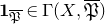



Before reading the upcoming definition, the reader is advised to recall the definition of viable ggtc space.
Definition 4.2. Let $\bigl ( Y=\coprod _{\eta \in T} Y_\eta ^\star ,(\mathcal{P}, {\bf 1}),\{\widehat {f_\eta }\mid \eta \in T\}\bigr )$
be a viable ggtc space.
$\bigl ( Y=\coprod _{\eta \in T} Y_\eta ^\star ,(\mathcal{P}, {\bf 1}),\{\widehat {f_\eta }\mid \eta \in T\}\bigr )$
be a viable ggtc space.
-
(1) A log structure compatible with the ggtc structure on
$Y$
, or simply a compatible log structure, is a log structure on
$Y$
over
$k^\dagger$
,
$\bigl ((Y, \mathfrak{P}), {\bf 1}_{\mathfrak{P}}\bigr )$
, together with a homomorphism of sheaves of monoidssuch that we have the following.
\begin{align*} \psi \colon \mathfrak{P} \to \mathcal{P} \end{align*}
-
(a) We have
$\psi ({\bf 1}_{\mathfrak{P}})={\bf 1}_{\mathcal{P}}$
and
$\psi$
induces an isomorphismof ghost sheaves. In particular,
\begin{align*} \overline {\psi } \colon \mathfrak{P}/\mathcal{O}_Y^\times = \overline {\mathfrak{P}} \overset {\cong }{\longrightarrow } \mathcal{P}\end{align*}
$\psi$
also induces an isomorphism
$\overline {\mathcal{M}}\to \mathcal{M}$
of the relative ghost sheaf of the log structure
$Y^\dagger /k^\dagger$
to the relative ghost sheaf of the ggtc space
$Y$
.
-
(b) For all
$y\in Y$
and
$p \in \mathfrak{P}_y$
, denote by
$[\psi (p)] \in \mathcal{M}_y$
the image of
$p$
, and let
$\tau \in \Sigma _y$
be the smallest cone that contains
$[\psi (p)]$
.Footnote
19
The condition is
$\alpha (p)\in \mathcal{O}_{Y, y}$
does not vanish identically on any component of
$\overline {U}_\tau \cap U_y$
, andwhere
\begin{align*} \operatorname {div} \left ( \alpha (p) \right ) = D_{\eta ,\tau } ([\psi (p)]) \quad \text{in} \ \operatorname {Div}^+_\flat \bigl ( \overline {U}_\tau \cap U_y \bigr ), \end{align*}
$\eta =b(y)$
and
$D_{\eta ,\tau } ([\psi (p)])$
is the Cartier divisor of Definition 2.16 (its existence guaranteed by the viability condition) and Notation 2.17.
-
-
(2) A morphism of compatible log structures
$(\mathfrak{P}, \psi )$
,
$(\mathfrak{P}^\prime ,\psi ^\prime )$
on
$Y$
is a morphism of log structures
$\varphi \colon \mathfrak{P} \to \mathfrak{P}^\prime$
such that for all sections
$p\in \mathfrak{P}$
,
$\psi (p)=\psi ^\prime (\varphi (p))$
. -
(3) We denote by
$\operatorname {LS}_{k^\dagger } (Y)$
the set of isomorphism classes of compatible log structures on
$Y$
.





Theorem 4.3.
Let $Y$
be a viable ggtc space, and let
$Y$
be a viable ggtc space, and let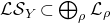 $\mathcal{LS}_Y\subset \bigoplus _\rho \mathcal{L}_\rho$
be the sheaf of Definition 3.9
.
$\mathcal{LS}_Y\subset \bigoplus _\rho \mathcal{L}_\rho$
be the sheaf of Definition 3.9
.
Denote by $\operatorname {LS}_{k^\dagger }(Y)$
the set of isomorphism classes of log structures on
$\operatorname {LS}_{k^\dagger }(Y)$
the set of isomorphism classes of log structures on $Y$
over
$Y$
over $k^\dagger$
compatible with the ggtc structure.
$k^\dagger$
compatible with the ggtc structure.
The set-theoretic function
 \begin{align*} r\colon \operatorname {LS}_{k^\dagger }(Y) \to \Gamma (Y,\mathcal{LS}_Y^\times ) \end{align*}
constructed in ( 4.15 ) is a bijection.
Next we give an outline of the proof. Details are carried out in the subsections that follow. In outline, our proof follows closely the proof of [Reference Gross and SiebertGS06, Theorem 3.22]; however, there are important differences due to the fact that we start out from an independent construction of the sheaf $\mathcal{LS}_Y$
.
$\mathcal{LS}_Y$
.
We conclude with a synopsis of the following subsections.
Outline of the proof of Theorem
4.3. Fix a viable ggtc space $Y$
as above. A compatible log structure
$Y$
as above. A compatible log structure $Y^\dagger =(Y, \mathfrak{P})$
sits in an extension sequence
$Y^\dagger =(Y, \mathfrak{P})$
sits in an extension sequence
 \begin{align*} 0 \to \mathcal{O}_Y^\times \to \mathfrak{P} \stackrel {\psi }\to \mathcal{P} \to 0. \end{align*}
Recall that the relative ghost sheaf $\mathcal{M}=\mathcal{P}/\textbf {1}_{\mathcal{P}}$
is a sheaf of groups. We have that
$\mathcal{M}=\mathcal{P}/\textbf {1}_{\mathcal{P}}$
is a sheaf of groups. We have that
 \begin{align*} \mathfrak{P}=\mathfrak{M} \times _{\mathcal{M}} \mathcal{P}, \end{align*}
where $\mathfrak{M}=\mathfrak{P}/{\bf 1}_{\mathfrak{P}}$
is a sheaf of abelian groupsFootnote
20
that is an extension in the category of sheaves of abelian groups on
$\mathfrak{M}=\mathfrak{P}/{\bf 1}_{\mathfrak{P}}$
is a sheaf of abelian groupsFootnote
20
that is an extension in the category of sheaves of abelian groups on $Y$
,
$Y$
,
 \begin{align*} 0 \to \mathcal{O}_Y^\times \to \mathfrak{M} \to \mathcal{M} \to 0. \end{align*}
The relative ghost sheaf $\mathcal{M}$
is supported in codimension one and
$\mathcal{M}$
is supported in codimension one and $Y$
is reduced, so
$Y$
is reduced, so $\mathcal{H}\!{\textit {om}}(\mathcal{M}, \mathcal{O}_Y^\times ) = 0$
. The local-to-global Ext spectral sequence then gives
$\mathcal{H}\!{\textit {om}}(\mathcal{M}, \mathcal{O}_Y^\times ) = 0$
. The local-to-global Ext spectral sequence then gives $\operatorname {Ext}^1(\mathcal{M}, \mathcal{O}_Y^\times ) = H^0\bigl (Y, \mathcal{E} \!{\textit {xt}}^1(\mathcal{M}, \mathcal{O}_Y^\times )\bigr )$
.
$\operatorname {Ext}^1(\mathcal{M}, \mathcal{O}_Y^\times ) = H^0\bigl (Y, \mathcal{E} \!{\textit {xt}}^1(\mathcal{M}, \mathcal{O}_Y^\times )\bigr )$
.
A key point of the proof is to characterize the extensions that give rise to compatible log structures. We introduce a subsheaf
 \begin{align*} \mathcal{E} \!{\textit {xt}}_c^1(\mathcal{M}, \mathcal{O}_Y^\times ) \subset \mathcal{E} \!{\textit {xt}}^1(\mathcal{M}, \mathcal{O}_Y^\times ) \end{align*}
which we call the sheaf of regular extensions, defined by a prescribed asymptotic behaviour at the boundary. This subsheaf is the same as the corresponding subsheaf defined in [Reference Gross and SiebertGS06] by fixing a ghost type. Here, we get around choosing local charts for the log structure by defining the intrinsic data of the local divisor system (Definition 4.12) and embedding it in the total ring of fractions.
The next step is to construct a sheaf homomorphism
 \begin{align*} \varphi \colon \mathcal{E} \!{\textit {xt}}_c^1(\mathcal{M}, \mathcal{O}_Y^\times )\to \mathcal{LS}^\times _Y. \end{align*}
Here we need to depart from [Reference Gross and SiebertGS06]: we introduce the local line bundle system (Definition 4.20) and construct $\varphi$
as an application of the abstract joint condition Lemma 3.6.
$\varphi$
as an application of the abstract joint condition Lemma 3.6.
While the proof of injectivity of $\varphi$
is very similar to [Reference Gross and SiebertGS06, Theorem 3.22], the proof of surjectivity departs somewhat from [Reference Gross and SiebertGS06]. It requires us to introduce
$\varphi$
is very similar to [Reference Gross and SiebertGS06, Theorem 3.22], the proof of surjectivity departs somewhat from [Reference Gross and SiebertGS06]. It requires us to introduce $2$
-homomorphisms from a lattice into the local line bundle system (Proposition 4.31), sections of these and then gluing them using the abstract joint condition once more.
$2$
-homomorphisms from a lattice into the local line bundle system (Proposition 4.31), sections of these and then gluing them using the abstract joint condition once more.
Finally, we construct
 \begin{align*} \psi \colon \operatorname {LS}_{k^\dagger }(Y) \to \mathcal{E} \!{\textit {xt}}_c^1(\mathcal{M}, \mathcal{O}_Y^\times ) \end{align*}
and prove that it is also bijective. Composing with $\varphi$
gives a bijection
$\varphi$
gives a bijection
 \begin{align*} r\colon \operatorname {LS}_{k^\dagger } (Y)\overset {\cong }{\longrightarrow }\mathcal{LS}^\times _Y.\end{align*}
This $2$
-homomorphism in the surjectivity of
$2$
-homomorphism in the surjectivity of $\varphi$
also plays a central role in the construction of a log structure from a section of
$\varphi$
also plays a central role in the construction of a log structure from a section of $\mathcal{LS}_Y$
, see Proposition 4.32. Our point of view in the proof of Proposition 4.32 closely matches that of [Reference Borne and VistoliBV12] as was pointed out to us by Bernd Siebert. A log structure in [Reference Borne and VistoliBV12] is defined as a certain symmetric monoidal functor. In fact, our
$\mathcal{LS}_Y$
, see Proposition 4.32. Our point of view in the proof of Proposition 4.32 closely matches that of [Reference Borne and VistoliBV12] as was pointed out to us by Bernd Siebert. A log structure in [Reference Borne and VistoliBV12] is defined as a certain symmetric monoidal functor. In fact, our $2$
-group
$2$
-group $\underline {T}(Y)$
of Section 4.5 agrees with the category
$\underline {T}(Y)$
of Section 4.5 agrees with the category $\operatorname {Div}(X)$
considered in [Reference Borne and VistoliBV12, Example 2.5].
$\operatorname {Div}(X)$
considered in [Reference Borne and VistoliBV12, Example 2.5].
Synopsis of the following sections.
In Section 4.2 we recall the basics of total rings of fractions and fractional ideals.
In Section 4.3 we work in the affine local situation $y\in Y$
and we construct a canonical resolution of
$y\in Y$
and we construct a canonical resolution of $\mathcal{M}$
(in the category of sheaves of abelian groups on
$\mathcal{M}$
(in the category of sheaves of abelian groups on $Y$
).
$Y$
).
In Section 4.4 we use this resolution to compute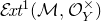 $\mathcal{E} \!{\textit {xt}}^1(\mathcal{M}, \mathcal{O}_Y^\times )$
in the affine local situation, and to define the subsheaf
$\mathcal{E} \!{\textit {xt}}^1(\mathcal{M}, \mathcal{O}_Y^\times )$
in the affine local situation, and to define the subsheaf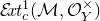 $\mathcal{E} \!{\textit {xt}}_c^1(\mathcal{M}, \mathcal{O}_Y^\times )$
. The local properties that define it in fact define it for every
$\mathcal{E} \!{\textit {xt}}_c^1(\mathcal{M}, \mathcal{O}_Y^\times )$
. The local properties that define it in fact define it for every $Y$
, not necessarily local.
$Y$
, not necessarily local.
In Section 4.5 we define a homomorphism $\varphi \colon \mathcal{E} \!{\textit {xt}}_c^1(\mathcal{M}, \mathcal{O}_Y^\times )\to \mathcal{LS}_Y$
in the affine local situation. In Section 4.6 we show that the definition globalizes to all
$\varphi \colon \mathcal{E} \!{\textit {xt}}_c^1(\mathcal{M}, \mathcal{O}_Y^\times )\to \mathcal{LS}_Y$
in the affine local situation. In Section 4.6 we show that the definition globalizes to all $Y$
, not necessarily local.
$Y$
, not necessarily local.
In Section 4.7 we show that $\varphi \colon \mathcal{E} \!{\textit {xt}}_c^1(\mathcal{M}, \mathcal{O}_Y^\times )\to \mathcal{LS}_Y$
is injective; in Section 4.8 we show that it is surjective.
$\varphi \colon \mathcal{E} \!{\textit {xt}}_c^1(\mathcal{M}, \mathcal{O}_Y^\times )\to \mathcal{LS}_Y$
is injective; in Section 4.8 we show that it is surjective.
In the final two sections we complete the proof of the main theorem: Section 4.9 does it in the affine local situation and Section 4.10 does it in the general case.
4.2 Sheaf of total ring of fractions and invertible fractional ideals
For a scheme $X$
, the sheaf of total rings of fractions
$X$
, the sheaf of total rings of fractions $\mathcal{K}_X$
is the sheafification of the presheaf
$\mathcal{K}_X$
is the sheafification of the presheaf $U\mapsto S(U)^{-1} \Gamma (U,\mathcal{O}_U)$
where
$U\mapsto S(U)^{-1} \Gamma (U,\mathcal{O}_U)$
where $S(U)\subset \Gamma (U,\mathcal{O}_U)$
is the subset of those non-zero-divisors of
$S(U)\subset \Gamma (U,\mathcal{O}_U)$
is the subset of those non-zero-divisors of $\Gamma (U,\mathcal{O}_U)$
that are also non-zero-divisors at every stalk of
$\Gamma (U,\mathcal{O}_U)$
that are also non-zero-divisors at every stalk of $\mathcal{O}_U$
. If
$\mathcal{O}_U$
. If $U$
is affine, then the stalk condition can be shown to be vacuous and
$U$
is affine, then the stalk condition can be shown to be vacuous and $S(U)$
is just the set of non-zero-divisors in
$S(U)$
is just the set of non-zero-divisors in $\Gamma (U,\mathcal{O}_U)$
, see p. 204 in [Reference KleimanKle79]. The case that concerns us is when
$\Gamma (U,\mathcal{O}_U)$
, see p. 204 in [Reference KleimanKle79]. The case that concerns us is when $X$
is a reduced scheme whose set of irreducible components is locally finite, case (b) on p. 205 in [Reference KleimanKle79]. In this case,
$X$
is a reduced scheme whose set of irreducible components is locally finite, case (b) on p. 205 in [Reference KleimanKle79]. In this case,
 \begin{align*}\mathcal{K}_X = j_*(\mathcal{O}_{X|\operatorname {Ass}(X)})\end{align*}
where $j\colon {\operatorname {Ass}}(X)\to X$
is the inclusion of the set of points
$j\colon {\operatorname {Ass}}(X)\to X$
is the inclusion of the set of points $x\in X$
for which the maximal ideal in
$x\in X$
for which the maximal ideal in $\mathcal{O}_{X,x}$
is associated to zero. The subsheaf of groups consisting of sections that are nowhere zero-divisors is denoted
$\mathcal{O}_{X,x}$
is associated to zero. The subsheaf of groups consisting of sections that are nowhere zero-divisors is denoted $\mathcal{K}_X^\times \subset \mathcal{K}_X$
.
$\mathcal{K}_X^\times \subset \mathcal{K}_X$
.
Example 4.4. Consider $X=\operatorname {Spec} A$
where
$X=\operatorname {Spec} A$
where $A=k[x,y]/(xy)$
, so
$A=k[x,y]/(xy)$
, so $X$
has irreducible components
$X$
has irreducible components $X_1=(y=0)$
and
$X_1=(y=0)$
and $X_2=(x=0)$
. For all
$X_2=(x=0)$
. For all $a,b\in k[x]$
,
$a,b\in k[x]$
, $c,d \in k[y]$
with
$c,d \in k[y]$
with $b,d\neq 0$
, consider the rational function
$b,d\neq 0$
, consider the rational function $f=\frac {ax+cy}{bx+dy} \in K(A)$
. Then
$f=\frac {ax+cy}{bx+dy} \in K(A)$
. Then $f_{\vert X_1}=\frac {a}b$
and
$f_{\vert X_1}=\frac {a}b$
and $f_{\vert X_2}=\frac {c}d$
, so
$f_{\vert X_2}=\frac {c}d$
, so $f=(\frac {a}b,\frac {c}d)$
under the natural isomorphism
$f=(\frac {a}b,\frac {c}d)$
under the natural isomorphism $K(A)=k(x) \times k(y)$
.
$K(A)=k(x) \times k(y)$
.
Following [EGA67, Sections 19–21], an invertible fractional ideal on a scheme $X$
is a coherent
$X$
is a coherent $\mathcal{O}_X$
-submodule
$\mathcal{O}_X$
-submodule $\mathcal{I} \subset \mathcal{K}_X$
that is locally principal. In other words, there is an affine cover of
$\mathcal{I} \subset \mathcal{K}_X$
that is locally principal. In other words, there is an affine cover of $X$
such that for all open subsets
$X$
such that for all open subsets $U=\operatorname {Spec} A\subset X$
that belong to this cover,
$U=\operatorname {Spec} A\subset X$
that belong to this cover,
 \begin{align} \mathcal{I}(U)=A\cdot \frac {s}{t}\subset \mathcal{K}_X(U) \end{align}
where $s,t$
are both non-zero-divisors in
$s,t$
are both non-zero-divisors in $A$
. The product of two fractional ideals inside
$A$
. The product of two fractional ideals inside $\mathcal{K}_X$
is again a fractional ideal giving the set of fractional ideals the structure of an abelian group. The sheaf of groups of fractional ideals on
$\mathcal{K}_X$
is again a fractional ideal giving the set of fractional ideals the structure of an abelian group. The sheaf of groups of fractional ideals on $X$
is denoted by
$X$
is denoted by $\mathcal{I} d.inv_X$
. The sheaf of Cartier divisors on
$\mathcal{I} d.inv_X$
. The sheaf of Cartier divisors on $X$
is, by definition, the sheaf of groups
$X$
is, by definition, the sheaf of groups
 \begin{align*} \mathcal{D} \!{\textit {iv}}_X = \mathcal{K}_X^\times /\mathcal{O}_X^\times. \end{align*}
The natural homomorphism $\mathcal{D} \!{\textit {iv}}_X\to \mathcal{I} d.inv_X$
is bijective [EGA67], Proposition (21.2.6). We denote by
$\mathcal{D} \!{\textit {iv}}_X\to \mathcal{I} d.inv_X$
is bijective [EGA67], Proposition (21.2.6). We denote by $\mathcal{D} \!{\textit {iv}}^+_X\subset \mathcal{D} \!{\textit {iv}}_X$
the subsheaf of those divisors whose invertible sheaf has local forms (4.1) with
$\mathcal{D} \!{\textit {iv}}^+_X\subset \mathcal{D} \!{\textit {iv}}_X$
the subsheaf of those divisors whose invertible sheaf has local forms (4.1) with $t=1$
. We set
$t=1$
. We set $\operatorname {Div} X=\Gamma (X,\mathcal{D} \!{\textit {iv}}_X)$
and
$\operatorname {Div} X=\Gamma (X,\mathcal{D} \!{\textit {iv}}_X)$
and $\operatorname {Div}^+\!X=\Gamma (X,\mathcal{D} \!{\textit {iv}}^+_X)$
.
$\operatorname {Div}^+\!X=\Gamma (X,\mathcal{D} \!{\textit {iv}}^+_X)$
.
4.3 The affine local situation
Setup 4.5. In this section we work with the following setup, which we refer to as the affine local situation:
-
(a)
$Y=\coprod _{\tau \in T} Y_\tau ^\star$
is an affine viable ggtc space; -
(b)
$Y$
has a unique smallest stratum
$Y_\eta ^\star = Y_\eta$
, which is necessarily closed; -
(c) we write
$M=M_\eta$
,
$\Sigma =\Sigma _\eta$
, etc.



The purpose of this section is to prove Lemma 4.8, giving a canonical resolution of the quotient sheaf
 \begin{align*} \mathcal{M} = \mathcal{P}^{\text{gp}}/{\bf 1}. \end{align*}
Recall $\mathcal{M}$
is so defined that, for a cone
$\mathcal{M}$
is so defined that, for a cone $\tau \in \Sigma$
the stalk
$\tau \in \Sigma$
the stalk $M_\tau$
is the quotient
$M_\tau$
is the quotient $M/\langle \tau \rangle$
(see Figure 3).
$M/\langle \tau \rangle$
(see Figure 3).
The stalks of the sheaf $\mathcal{M}=\mathcal{P}^{\text{gp}}/{\bf 1}$
at various points of
$\mathcal{M}=\mathcal{P}^{\text{gp}}/{\bf 1}$
at various points of $T$
for the normal crossing surface
$T$
for the normal crossing surface $xyz=0$
.
$xyz=0$
.
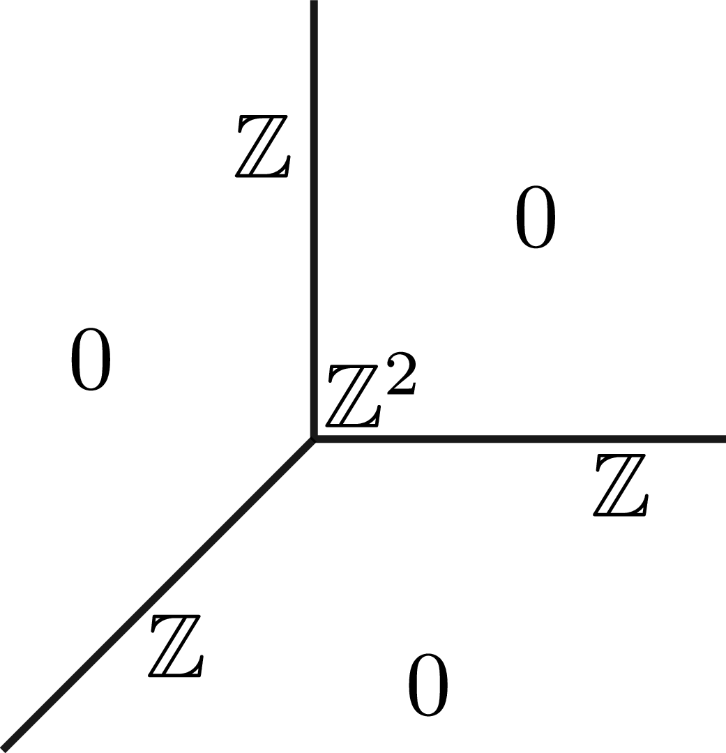
Figure 3. Long description
The equation displays a three-dimensional coordinate system with variables Z and 0. The axes are labeled with Z, Z squared, and 0 in different planes.
Notation 4.6. For all $\tau \in \Sigma$
, denote by
$\tau \in \Sigma$
, denote by $\underline {\langle \tau \rangle }_{U_\tau }$
the constant sheaf on
$\underline {\langle \tau \rangle }_{U_\tau }$
the constant sheaf on $U_\tau$
with group
$U_\tau$
with group $\langle \tau \rangle$
. Denoting by
$\langle \tau \rangle$
. Denoting by $j_\tau \colon U_\tau \hookrightarrow Y$
the inclusion, we write
$j_\tau \colon U_\tau \hookrightarrow Y$
the inclusion, we write
 \begin{align*} L_!(\tau )=j_{\tau \, !} \underline {\langle \tau \rangle }_{U_\tau } ,\end{align*}
where $j_{\tau \, !}$
is the extension by zero. More explicitly, if
$j_{\tau \, !}$
is the extension by zero. More explicitly, if $U\subset Y$
is a connected open subset, we have
$U\subset Y$
is a connected open subset, we have
 \begin{align*} L_!(\tau ) (U)= \begin{cases} \langle \tau \rangle \quad & \text{if $U\subset U_\tau $}, \\ 0 \quad & \text{otherwise.} \end{cases} \end{align*}
Construction 4.7. Recall that for an open embedding $j\colon U\to U'$
, we have
$j\colon U\to U'$
, we have $j^*=j^!$
and hence for a sheaf
$j^*=j^!$
and hence for a sheaf $\mathcal{F}$
on
$\mathcal{F}$
on $U'$
, we have an adjunction morphism
$U'$
, we have an adjunction morphism $j_!j^*\mathcal{F}\to \mathcal{F}$
. With that in mind, and using that, for
$j_!j^*\mathcal{F}\to \mathcal{F}$
. With that in mind, and using that, for $\tau _1\lt \tau _2$
, the open embedding
$\tau _1\lt \tau _2$
, the open embedding $j_{\tau _2}\colon U_{\tau _2}\to Y$
factors through
$j_{\tau _2}\colon U_{\tau _2}\to Y$
factors through $j_{\tau _1}\colon U_{\tau _1}\to Y$
, we have a natural map
$j_{\tau _1}\colon U_{\tau _1}\to Y$
, we have a natural map
 \begin{align*} d_{\tau _1\tau _2}\colon j_{\tau _1\, !} \underline {\langle \tau _1 \rangle }_{U_{\tau _1}} \to j_{\tau _2\, !} \underline {\langle \tau _2 \rangle }_{U_{\tau _2}} \end{align*}
which at a stalk of a point $p\in Y$
is either the natural inclusion
$p\in Y$
is either the natural inclusion $\langle \tau _1 \rangle \subset \langle \tau _2 \rangle$
or the zero map, depending on whether
$\langle \tau _1 \rangle \subset \langle \tau _2 \rangle$
or the zero map, depending on whether $p\in U_{\tau _2}$
or not. We define a homomorphism
$p\in U_{\tau _2}$
or not. We define a homomorphism
 \begin{align*}\delta _i\colon \bigoplus _{\tau _0\lneq \ldots \lneq \tau _i} L_!(\tau _i)\to \bigoplus _{\tau _0\lneq \ldots \lneq \tau _{i-1}} L_!(\tau _{i-1}) \end{align*}
via $\delta _i(\sum _{\tau _0\lneq \ldots \lneq \tau _i} a_{\tau _0\lneq \ldots \lneq \tau _i})=\sum _{\tau _0\lneq \ldots \lneq \tau _i} \delta _i(a_{\tau _0\lneq \ldots \lneq \tau _i})$
and a component of
$\delta _i(\sum _{\tau _0\lneq \ldots \lneq \tau _i} a_{\tau _0\lneq \ldots \lneq \tau _i})=\sum _{\tau _0\lneq \ldots \lneq \tau _i} \delta _i(a_{\tau _0\lneq \ldots \lneq \tau _i})$
and a component of $\delta _i(a_{\tau _0\lneq \ldots \lneq \tau _i})$
is trivial except for
$\delta _i(a_{\tau _0\lneq \ldots \lneq \tau _i})$
is trivial except for
 \begin{align*}\delta _i(a_{\tau _0\lneq \ldots \lneq \tau _i})_{{\tau _0\lneq \ldots \widehat \tau _j\ldots \lneq \tau _{i}}} =(-1)^j a_{\tau _0\lneq \ldots \lneq \tau _i},\end{align*}
where $\tau _0\lneq \ldots \widehat \tau _j\ldots \lneq \tau _{i}$
refers to the result of removing
$\tau _0\lneq \ldots \widehat \tau _j\ldots \lneq \tau _{i}$
refers to the result of removing $\tau _j$
from the sequence
$\tau _j$
from the sequence $\tau _0\lneq \ldots \lneq \tau _{i}$
for
$\tau _0\lneq \ldots \lneq \tau _{i}$
for $0\le j\lt i$
; and for
$0\le j\lt i$
; and for
 \begin{align*} \delta _i(a_{\tau _0\lneq \ldots \lneq \tau _i})_{{\tau _0\lneq \ldots \lneq \tau _{i-1}}} =(-1)^i d_{\tau _{i-1}\tau _i}(a_{\tau _0\lneq \ldots \lneq \tau _{i}}). \end{align*}
In particular,
 \begin{align} \delta _1\left (\sum _{\tau _0\lneq \tau _1} a_{\tau _0\lneq \tau _1}\right )_{\tau }= \sum _{\tau _0\lneq \tau } a_{\tau _0\lneq \tau } - \sum _{\tau \lneq \tau _1} d_{\tau \tau _1}(a_{\tau \lneq \tau _{1}}). \end{align}
Lemma 4.8.
Let $\underline {M}$
denote the constant sheaf on
$\underline {M}$
denote the constant sheaf on $Y$
with group
$Y$
with group $M$
. Construction 4.7 gives a resolution of
$M$
. Construction 4.7 gives a resolution of $\mathcal{M}$
by sheaves on
$\mathcal{M}$
by sheaves on $Y$
:
$Y$
:
 \begin{align*} \cdots \to \bigoplus _{\tau _0\leqslant \tau _1} L_!(\tau _1) \stackrel {\delta _1}\longrightarrow \bigoplus _{\tau \in \Sigma } L_!(\tau ) \stackrel {\delta _0}\longrightarrow \underline {M} \to \mathcal{M} \to 0. \end{align*}
Proof.
Exactness is to be checked at the stalk level, so let us fix a point $p\in Y$
. The complex of stalks only depends on the stratum
$p\in Y$
. The complex of stalks only depends on the stratum $Y_\tau ^\star$
that contains
$Y_\tau ^\star$
that contains $p$
. We have
$p$
. We have $p\in U_{\tau '}$
if an only if
$p\in U_{\tau '}$
if an only if $\tau '\lt \tau$
. In particular,
$\tau '\lt \tau$
. In particular, $L_!(\tau ')_p=0$
unless
$L_!(\tau ')_p=0$
unless $\tau '\lt \tau$
. The complex has an increasing filtration
$\tau '\lt \tau$
. The complex has an increasing filtration $F_k$
by subcomplexes given by requiring the maximum for the dimension of the cones in the the chain
$F_k$
by subcomplexes given by requiring the maximum for the dimension of the cones in the the chain $\tau _0\lneq \ldots \lneq \tau _i$
to be at most
$\tau _0\lneq \ldots \lneq \tau _i$
to be at most $k$
, that is,
$k$
, that is, $\dim \tau _i\le k$
. To show the exactness of the original sequence, it suffices to show the exactness of the graded quotients with respect to the filtration. The graded quotient decomposes as
$\dim \tau _i\le k$
. To show the exactness of the original sequence, it suffices to show the exactness of the graded quotients with respect to the filtration. The graded quotient decomposes as $F_k / F_{k-1} = \bigoplus _{\dim \tau =k} C_{\tau }$
and
$F_k / F_{k-1} = \bigoplus _{\dim \tau =k} C_{\tau }$
and $C_{\tau }$
is the complex that result from applying
$C_{\tau }$
is the complex that result from applying $L_!(\tau )\otimes \cdot$
to the complex
$L_!(\tau )\otimes \cdot$
to the complex
 \begin{align*} \cdots \to \bigoplus _{\tau _0\lneq \ldots \lneq \tau _i=\tau }\mathbb{Z}\to \cdots \to \bigoplus _{\tau _0\lneq \tau _1=\tau } \to \mathbb{Z}\end{align*}
with differential similar to $\delta _i$
as before. This complex is exact, as it can be identified with the augmented chain complex for the homology of a contractible space.
$\delta _i$
as before. This complex is exact, as it can be identified with the augmented chain complex for the homology of a contractible space.
Definition 4.9. The relation sheaf is the sheaf $\mathcal{R}$
on
$\mathcal{R}$
on $Y$
defined by the exact sequence:
$Y$
defined by the exact sequence:
 \begin{align} 0 \to \mathcal{R} \to \underline {M} \to \mathcal{M} \to 0. \end{align}
See Figure 4 for an illustration of the relation sheaf.
4.4 The sheaf
$\mathcal{E} \!{\textit {xt}}_c^1(\mathcal{M}, \mathcal{O}_Y^\times )$
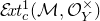
Setup 4.10. We continue with the affine local situation of Setup 4.5.
In this section we define a subsheaf $\mathcal{E} \!{\textit {xt}}_c^1(\mathcal{M}, \mathcal{O}_Y^\times ) \subset \mathcal{E} \!{\textit {xt}}^1(\mathcal{M}, \mathcal{O}_Y^\times )$
, which we call the sheaf of regular extensions, consisting of sections with a prescribed asymptotic behaviour towards the Zariski closure
$\mathcal{E} \!{\textit {xt}}_c^1(\mathcal{M}, \mathcal{O}_Y^\times ) \subset \mathcal{E} \!{\textit {xt}}^1(\mathcal{M}, \mathcal{O}_Y^\times )$
, which we call the sheaf of regular extensions, consisting of sections with a prescribed asymptotic behaviour towards the Zariski closure $\overline {U}_\tau$
of
$\overline {U}_\tau$
of $U_\tau$
in
$U_\tau$
in $Y$
. Before we can state this definition, we need to discuss some preliminaries.
$Y$
. Before we can state this definition, we need to discuss some preliminaries.
The stalks of the relation sheaf $\mathcal{R}$
at various points of
$\mathcal{R}$
at various points of $T$
for the normal crossing surface
$T$
for the normal crossing surface $xyz=0$
.
$xyz=0$
.
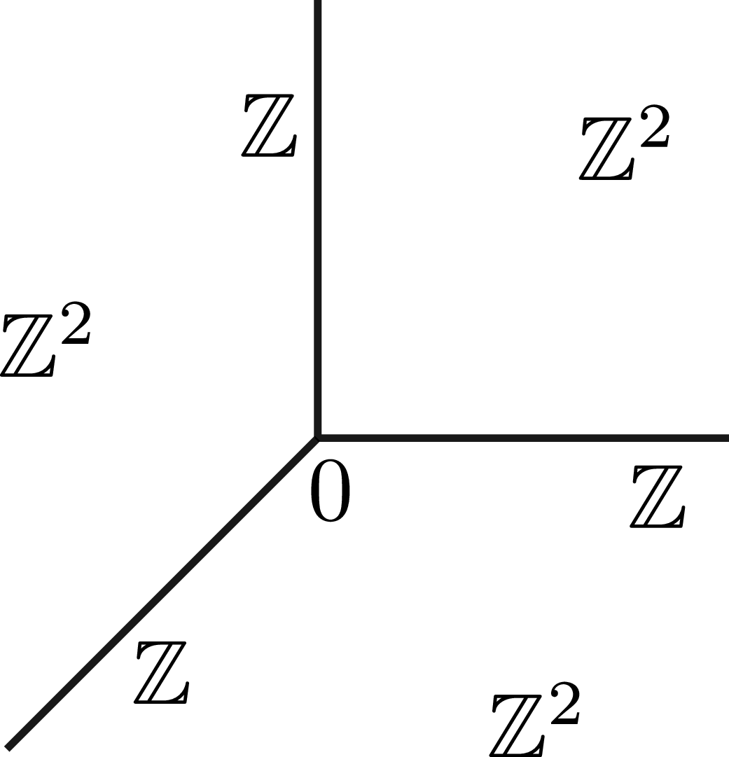
Lemma 4.11.
For all cones $\tau ^\prime \leqslant \tau$
in
$\tau ^\prime \leqslant \tau$
in $\Sigma$
, denote by
$\Sigma$
, denote by $\rho ^{\tau ^\prime }_{\tau }\colon \mathcal{O}_Y^\times (U_{\tau ^\prime })\to \mathcal{O}_Y^\times (U_{\tau })$
the restriction homomorphism.
$\rho ^{\tau ^\prime }_{\tau }\colon \mathcal{O}_Y^\times (U_{\tau ^\prime })\to \mathcal{O}_Y^\times (U_{\tau })$
the restriction homomorphism.
We have the following concrete description of the relation sheaf: for every open $U\subset Y$
 \begin{align} & \Gamma (U, \mathcal{H}\!{\textit {om}} (\mathcal{R}, \mathcal{O}_Y^\times )) = \left \{\left . h\in \mathcal{H}\!{\textit {om}} \left ( \bigoplus _\tau L_!(\tau ),\mathcal{O}_Y^\times \right )(U)\,\right |\, h_{|\operatorname {im}\delta _1}=0\right \}\nonumber \\ & =\left \{ \left (h_\tau \right )_{\tau \in \Sigma } \left | \begin{array}{l} h_\tau \colon \langle \tau \rangle \to \mathcal{O}_Y(U\cap U_\tau )^\times \;\text{ is a group homomorphism}\\ \text{and for every }\tau ^\prime \leqslant \tau \text{ we have } \rho ^{\tau ^\prime }_{\tau } \circ h_{\tau ^\prime } = h_{\tau | \langle \tau ^\prime \rangle } \end{array} \right. \right \}. \end{align}
Proof.
Straightforward from Lemma 4.8 and the adjoint properties of the functor $j_!$
.
$j_!$
.
Definition 4.12. The local divisor system is the system of group homomorphisms $\{D_{\eta ,\tau } |\tau \in \Sigma \}$
where, for all
$\{D_{\eta ,\tau } |\tau \in \Sigma \}$
where, for all $\tau \in \Sigma$
,
$\tau \in \Sigma$
,
 \begin{align*} D_{\eta ,\tau } \colon \langle \tau \rangle \to \operatorname {Div} \overline {U}_\tau \end{align*}
is the group homomorphism of Definition 2.16 and Notation 2.17.
Notation 4.13. Because in this section $\eta \in T$
is the unique smallest stratum, in this section we suppress the subscript
$\eta \in T$
is the unique smallest stratum, in this section we suppress the subscript $\eta$
from the notation and simply write
$\eta$
from the notation and simply write $D_\tau$
instead of
$D_\tau$
instead of $D_{\eta , \tau }$
.
$D_{\eta , \tau }$
.
Lemma 4.14. The local divisor system satisfies the conditions (A), (B) and (C) given below.
Note that if $\tau ^\prime \leqslant \tau$
, then
$\tau ^\prime \leqslant \tau$
, then $U_{\tau ^\prime } \supset U_\tau$
. In the statement of the conditions we denote by
$U_{\tau ^\prime } \supset U_\tau$
. In the statement of the conditions we denote by $\overline \rho ^{\tau ^\prime }_{\tau } \colon \operatorname {Div} \overline {U}_{\tau ^\prime } \to \operatorname {Div} \overline {U}_{\tau }$
the restriction of Cartier divisors: this restriction is defined because
$\overline \rho ^{\tau ^\prime }_{\tau } \colon \operatorname {Div} \overline {U}_{\tau ^\prime } \to \operatorname {Div} \overline {U}_{\tau }$
the restriction of Cartier divisors: this restriction is defined because $\overline {U}_\tau$
is a union of irreducible components of
$\overline {U}_\tau$
is a union of irreducible components of $\overline {U}_{\tau ^\prime }$
. Figure 5 gives an illustration.
$\overline {U}_{\tau ^\prime }$
. Figure 5 gives an illustration. $\overline {U}_{\tau }\subset \overline {U}_{\tau '}$
for
$\overline {U}_{\tau }\subset \overline {U}_{\tau '}$
for $\tau ^\prime \leqslant \tau$
.
$\tau ^\prime \leqslant \tau$
.
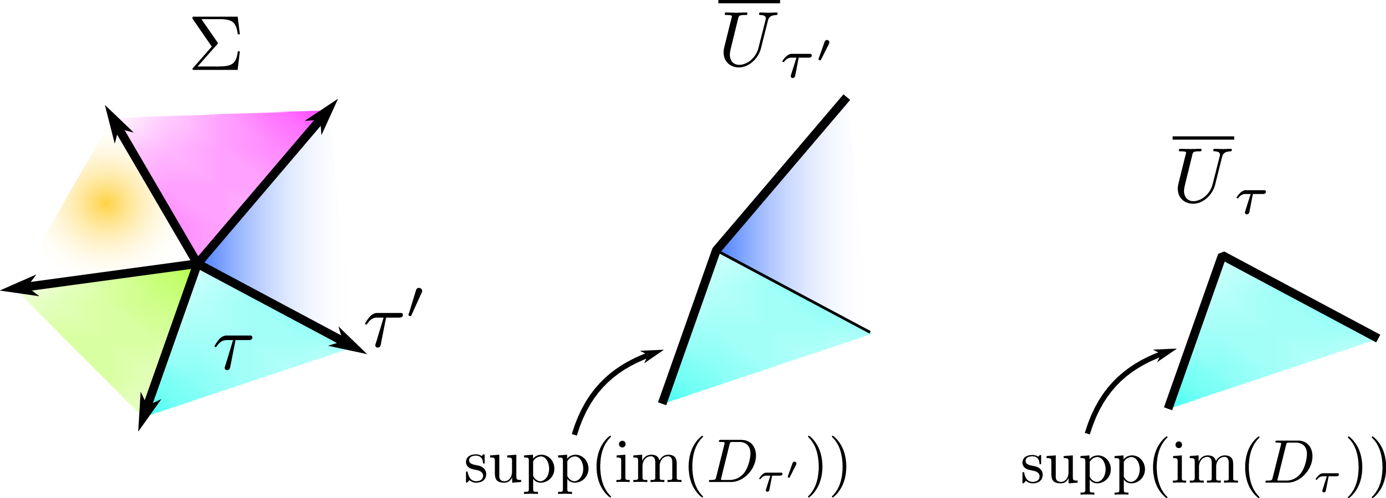
Figure 5. Long description
The illustration features geometric shapes divided into colored sections, labeled with mathematical symbols such as Σ, T, and U. Arrows indicate relationships between these shapes, suggesting transformations or mappings. The notations and arrows likely represent log structures and their resolutions in a mathematical context, hinting at complex theoretical concepts related to singular log structures and log crepant log resolutions.
The conditions are as follows.
-
(A) Fan property. If
$\tau ^\prime \leqslant \tau$
, then
\begin{align*} \overline \rho ^{\tau ^\prime }_{\tau } \circ D_{\tau ^\prime } = D_{\tau |\langle \tau ^\prime \rangle }.\end{align*}
-
(B) Positivity. We have
$D_\tau (\langle \tau \rangle _+) \subset \operatorname {Div}^+ \overline {U}_\tau$
. -
(C) Support property. The composition of
$D_\tau$
with the restriction
$\operatorname {Div} \overline {U}_\tau \to \operatorname {Div} U_\tau$
gives the trivial map. In particular, none of the divisors in
$D_\tau (\langle \tau \rangle )$
contain the stratum
$Y_\tau$
in their support; hence all of these divisors are restrictable to
$Y_\tau$
.







Proof.
The statement is a straightforward consequence of the definition. By construction of $D$
, see Definition 2.16, we may assume that
$D$
, see Definition 2.16, we may assume that $Y=\operatorname {Spec} k(\eta ) [\Sigma _y]$
with
$Y=\operatorname {Spec} k(\eta ) [\Sigma _y]$
with $D_\tau (m)=\operatorname {div} z^m$
, where the result is basically obvious.
$D_\tau (m)=\operatorname {div} z^m$
, where the result is basically obvious.
Part (A) follows from observing that for $m\in \tau '$
, by definition,
$m\in \tau '$
, by definition, $D_{\tau '}(m)=\operatorname {div} z^m\in \operatorname {Div} \overline {\Omega }_{\tau '}$
and so
$D_{\tau '}(m)=\operatorname {div} z^m\in \operatorname {Div} \overline {\Omega }_{\tau '}$
and so $\overline \rho ^{\tau ^\prime }_{\tau } \circ D_{\tau '}(m)$
is its restriction to
$\overline \rho ^{\tau ^\prime }_{\tau } \circ D_{\tau '}(m)$
is its restriction to $\overline {\Omega }_{\tau }$
which of course agrees with
$\overline {\Omega }_{\tau }$
which of course agrees with $D_{\tau }(m)=\operatorname {div} z^m\in \operatorname {Div} \overline {\Omega }_{\tau }$
.
$D_{\tau }(m)=\operatorname {div} z^m\in \operatorname {Div} \overline {\Omega }_{\tau }$
.
Part (B) is clear because $D_{\tau }(m)=\operatorname {div} z^m$
is a principal divisor of a regular function.
$D_{\tau }(m)=\operatorname {div} z^m$
is a principal divisor of a regular function.
Moreover, since $z^m$
is invertible on
$z^m$
is invertible on $\Omega _\tau$
for
$\Omega _\tau$
for $m\in \tau$
, its support is contained in
$m\in \tau$
, its support is contained in $\overline {\Omega }_{\tau }\setminus \Omega _\tau$
, so we deduce part (C).
$\overline {\Omega }_{\tau }\setminus \Omega _\tau$
, so we deduce part (C).
We are now ready to define the subsheaf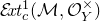 $\mathcal{E} \!{\textit {xt}}_c^1(\mathcal{M}, \mathcal{O}_Y^\times )$
. As in Section 4.2, we denote by
$\mathcal{E} \!{\textit {xt}}_c^1(\mathcal{M}, \mathcal{O}_Y^\times )$
. As in Section 4.2, we denote by $\mathcal{K}_Y$
be the sheaf of total rings of fractions on
$\mathcal{K}_Y$
be the sheaf of total rings of fractions on $Y$
and a Cartier divisor
$Y$
and a Cartier divisor $D$
on
$D$
on $Y$
gives the subsheaf
$Y$
gives the subsheaf $\mathcal{O}_Y (D)\subset \mathcal{K}_Y$
.
$\mathcal{O}_Y (D)\subset \mathcal{K}_Y$
.
Definition 4.15.
-
(1) Let
$U\subset Y$
be an open subset, and consider a section
$(h_\tau )_{\tau \in \Sigma }\in \Gamma (U,\mathcal{H}\!{\textit {om}} (\mathcal{R}, \mathcal{O}_Y^\times ))$
. Denote by
$\widetilde {h}_\tau \colon \langle \tau \rangle \to \mathcal{K}_Y (\overline {U}_\tau \cap U)$
the composition of
$h_\tau \colon \langle \tau \rangle \to \mathcal{O}_Y^\times (U_\tau \cap U)$
with the inclusion
$\mathcal{O}_Y^\times (U_\tau \cap U)\hookrightarrow \mathcal{K}_Y(\overline {U}_\tau \cap U)$
.We say that
$h$
is regular if for all
$\tau \in \Sigma$
and
$m\in \tau$
,
$\widetilde {h}_\tau (m)$
is a generator of
$\mathcal{O}_{\overline {U}_\tau \cap U} \bigl ( -D_\tau (m)\bigr ) \subset \mathcal{K}_{\overline {U}_\tau \cap U}$
as a
$\mathcal{O}_{\overline {U}_\tau \cap U}$
-module. We denote bythe subsheaf of regular sections.
\begin{align*} \mathcal{H}\!{\textit {om}}_c (\mathcal{R}, \mathcal{O}_Y^\times ) \subset \mathcal{H}\!{\textit {om}} (\mathcal{R}, \mathcal{O}_Y^\times ) \end{align*}
-
(2) Consider the exact sequence:
(4.5)The sheaf of regular extensions, denoted by
\begin{align} \mathcal{H}\!{\textit {om}}(\underline {M}, \mathcal{O}_Y^\times ) \to \mathcal{H}\!{\textit {om}} (\mathcal{R}, \mathcal{O}_Y^\times ) \to \mathcal{E} \!{\textit {xt}}^1(\mathcal{M}, \mathcal{O}_Y^\times ) \to 0. \end{align}
$\mathcal{E} \!{\textit {xt}}_c^1 (\mathcal{M}, \mathcal{O}_Y^\times )$
, is the image of
$\mathcal{H}\!{\textit {om}}_c (\mathcal{R}, \mathcal{O}_Y^\times )$
in
$\mathcal{E} \!{\textit {xt}}^1(\mathcal{M}, \mathcal{O}_Y^\times )$
.










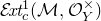

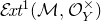
4.5 A morphism
$\varphi \colon \mathcal{E} \!{\textit {xt}}_c^1 (\mathcal{M}, \mathcal{O}_Y^\times ) \to \mathcal{LS}_Y$
in the affine local situation

Setup 4.16. We continue with the affine local situation of Setup 4.5, and we assume in addition the following.
-
(d) For all
$\tau \in \Sigma$
, and all
$m\in \tau$
,
$\mathcal{O}(-D_\tau (m))$
is a trivial line bundle on
$\overline {U}_\tau$
.


Construction 4.17. Let $U\subset Y$
be open and
$U\subset Y$
be open and $h\in \Gamma (U,\mathcal{E} \!{\textit {xt}}_c^1 (\mathcal{M}, \mathcal{O}_Y^\times ))$
. Because of assumption (d) of Setup 4.16,
$h\in \Gamma (U,\mathcal{E} \!{\textit {xt}}_c^1 (\mathcal{M}, \mathcal{O}_Y^\times ))$
. Because of assumption (d) of Setup 4.16, $h$
lifts to
$h$
lifts to
 \begin{align*} (h_\tau )_{\tau \in \Sigma }\in \mathcal{H}\!{\textit {om}}_c (\mathcal{R}, \mathcal{O}_Y^\times )(U). \end{align*}
Consider two maximal cones $\sigma _1, \sigma _2\in \Sigma$
meeting along a common facet
$\sigma _1, \sigma _2\in \Sigma$
meeting along a common facet $\rho$
. We choose
$\rho$
. We choose $e_2\in (\langle \rho \rangle + \sigma _2)\cap M$
at integral distance
$e_2\in (\langle \rho \rangle + \sigma _2)\cap M$
at integral distance $1$
from
$1$
from $\rho$
and setFootnote
21
$\rho$
and setFootnote
21
 \begin{align} \varphi _\rho (h) = {\widetilde {h}_{\sigma _1}(e_2)}_{|Y_\rho } \otimes {\widetilde {h}_{\sigma _2} (-e_2)}_{|Y_\rho } \end{align}
and the regularity of $h$
implies that
$h$
implies that $\varphi _\rho (h)$
is a generator of the chart
$\varphi _\rho (h)$
is a generator of the chart
 \begin{align} \lambda _\rho (e_2)= {\mathcal{O}_{U_1}\bigl (D_{\sigma _1} (-e_2)\bigr )}_{|Y_\rho } \otimes {\mathcal{O}_{U_2}\bigl (D_{\sigma _2} (e_2)\bigr )}_{|Y_\rho } \end{align}
of the line bundle $\mathcal{L}_{\rho | U}$
.
$\mathcal{L}_{\rho | U}$
.
Lemma-Definition 4.18.
Let $U\subset Y$
be open and
$U\subset Y$
be open and $h\in \Gamma (U, \mathcal{E} \!{\textit {xt}}_c^1 (\mathcal{M}, \mathcal{O}_Y^\times ))$
.
$h\in \Gamma (U, \mathcal{E} \!{\textit {xt}}_c^1 (\mathcal{M}, \mathcal{O}_Y^\times ))$
.
-
(1) The section
$\varphi _\rho (h) \in \Gamma (Y_\rho \cap U,\mathcal{L}_\rho )$
of Construction 4.17 does not depend on the choice of the lift
$(h_\tau )_{\tau \in \Sigma }\in \mathcal{H}\!{\textit {om}}_c (\mathcal{R}, \mathcal{O}_Y^\times )(U)$
, nor on the choice of
$e_2$
. Thus, Construction 4.17 provides for all
$\rho \in T^{[1]}$
a morphism of sheaves
\begin{align*} \varphi _\rho \colon \mathcal{E} \!{\textit {xt}}_c^1 (\mathcal{M}, \mathcal{O}_Y^\times ) \to \mathcal{L}_\rho. \end{align*}
-
(2) Assembling the morphisms of part (1) gives a morphism
$\textstyle \bigoplus _{\rho \in T^{[1]}} \varphi _\rho \colon \mathcal{E} \!{\textit {xt}}_c^1 (\mathcal{M}, \mathcal{O}_Y^\times ) \to \bigoplus _{\rho \in T^{[1]}}\mathcal{L}_\rho$
. The image of this morphism lies in
$\mathcal{LS}_Y^\times$
.






The two parts show that Construction 4.17 provides a morphism $\varphi \colon \mathcal{E} \!{\textit {xt}}_c^1 (\mathcal{M}, \mathcal{O}_Y^\times ) \to \mathcal{LS}_Y^\times$
.
$\varphi \colon \mathcal{E} \!{\textit {xt}}_c^1 (\mathcal{M}, \mathcal{O}_Y^\times ) \to \mathcal{LS}_Y^\times$
.
Beginning of the proof of Lemma-Definition
4.18. We show that $\varphi (h)_\rho$
does not depend on the choice of lift
$\varphi (h)_\rho$
does not depend on the choice of lift $(h_\tau )_{\tau \in \Sigma }\in \mathcal{H}\!{\textit {om}}_c (\mathcal{R}, \mathcal{O}_Y^\times )(U)$
and also that it does not depend on the choice of
$(h_\tau )_{\tau \in \Sigma }\in \mathcal{H}\!{\textit {om}}_c (\mathcal{R}, \mathcal{O}_Y^\times )(U)$
and also that it does not depend on the choice of $e_2$
. Another choice of lift differs from the chosen one by an element
$e_2$
. Another choice of lift differs from the chosen one by an element
 \begin{align*} u\in \mathcal{H}\!{\textit {om}} (\underline {M} , \mathcal{O}_Y^\times )(U) = \operatorname {Hom}_{\text{groups}}(M, \mathcal{O}_Y(U)^\times ), \end{align*}
so it can be written as $(uh_\tau )_{\tau \in \Sigma }$
and then
$(uh_\tau )_{\tau \in \Sigma }$
and then
 \begin{align*} \varphi (uh)_\rho ={\bigl (u(e_2) \widetilde {h}_{\sigma _1}(e_2)\bigr )}_{|Y_\rho } \otimes {\bigl (u(e_2)^{-1}\widetilde {h}_{\sigma _2} (-e_2)\bigr )}_{|Y_\rho } \end{align*}
agrees with $\varphi (h)_\rho$
.
$\varphi (h)_\rho$
.
A different choice $e'_2$
of
$e'_2$
of $e_2$
differs by
$e_2$
differs by $r=e_2'-e_2\in \langle \rho \rangle$
and leads to a different chart
$r=e_2'-e_2\in \langle \rho \rangle$
and leads to a different chart $\lambda _\rho (e_2^\prime )$
of
$\lambda _\rho (e_2^\prime )$
of $\mathcal{L}_\rho$
which is isomorphic to the one in (4.7) via the isomorphism
$\mathcal{L}_\rho$
which is isomorphic to the one in (4.7) via the isomorphism $\psi _r$
from Lemma 3.2. It is straightforward to see that the assignment of the section
$\psi _r$
from Lemma 3.2. It is straightforward to see that the assignment of the section $\varphi (h)_\rho$
to the tuple
$\varphi (h)_\rho$
to the tuple $(h_\tau )_{\tau \in \Sigma }$
is compatible with
$(h_\tau )_{\tau \in \Sigma }$
is compatible with $\psi _r$
.
$\psi _r$
.
We have thus constructed a morphisms of sheaves of sets $\oplus _{\rho } \varphi _\rho \colon \mathcal{E} \!{\textit {xt}}_c^1 (\mathcal{M}, \mathcal{O}_Y^\times ) \to \bigoplus _\rho \mathcal{L}_\rho$
. We next explain why its image is contained in
$\oplus _{\rho } \varphi _\rho \colon \mathcal{E} \!{\textit {xt}}_c^1 (\mathcal{M}, \mathcal{O}_Y^\times ) \to \bigoplus _\rho \mathcal{L}_\rho$
. We next explain why its image is contained in $\mathcal{LS}^\times _Y$
, i.e., why its elements are nowhere-vanishing and satisfy the joint condition. That they are nowhere-vanishing follows immediately from the regularity property.
$\mathcal{LS}^\times _Y$
, i.e., why its elements are nowhere-vanishing and satisfy the joint condition. That they are nowhere-vanishing follows immediately from the regularity property.
Before showing that the joint condition holds we need to discuss some preliminaries.
Definition 4.19. Let $X$
be a space. The
$X$
be a space. The $2$
-group
$2$
-group $\underline {T} (X)$
of trivialized line bundles on
$\underline {T} (X)$
of trivialized line bundles on $X$
is the strictly commutative
$X$
is the strictly commutative $2$
-group where:
$2$
-group where:
-
– objects of
$\underline {T} (X)$
are trivialized line bundles on
$X$
, that is, pairs
$(\mathcal{L}, s)$
where
$\mathcal{L}$
is a (trivial) line bundle on
$X$
, and
$s\colon \mathcal{O}_X\to \mathcal{L}$
an isomorphism; -
– a morphism from
$(\mathcal{L}_1, s_1)$
to
$(\mathcal{L}_2,s_2)$
is an isomorphisms
$s\colon \mathcal{L}_1\to \mathcal{L}_2$
such that
$s_2=s\circ s_1$
.


The monoidal structure in $\underline {T} (X)$
is given by tensor product
$\underline {T} (X)$
is given by tensor product
 \begin{align*} (\mathcal{L}_1,s_1)(\mathcal{L}_2, s_2)=(\mathcal{L}_1\otimes \mathcal{L}_2, s_1\otimes s_2) \end{align*}
and the distinguished neutral element is the trivial line bundle $\mathcal{O}_X$
with the unit trivializing section
$\mathcal{O}_X$
with the unit trivializing section $1$
. For
$1$
. For $(\mathcal{L},s)$
we have the inverse
$(\mathcal{L},s)$
we have the inverse $(\mathcal{L}^\star ,(s^\star )^{-1})$
where
$(\mathcal{L}^\star ,(s^\star )^{-1})$
where $\mathcal{L}^\star =\mathcal{H}\!{\textit {om}}(\mathcal{L},\mathcal{O}_X)$
denotes the dual and
$\mathcal{L}^\star =\mathcal{H}\!{\textit {om}}(\mathcal{L},\mathcal{O}_X)$
denotes the dual and $s^\star$
the dual map. For any pair
$s^\star$
the dual map. For any pair $(\mathcal{L}_1, s_1),(\mathcal{L}_2,s_2)\in \underline {T} (X)$
, there is a unique morphism
$(\mathcal{L}_1, s_1),(\mathcal{L}_2,s_2)\in \underline {T} (X)$
, there is a unique morphism $(\mathcal{L}_1, s_1)\to (\mathcal{L}_2,s_2)$
in
$(\mathcal{L}_1, s_1)\to (\mathcal{L}_2,s_2)$
in $\underline {T} (X)$
, so, in particular, we have unique morphisms
$\underline {T} (X)$
, so, in particular, we have unique morphisms
 \begin{align*} (\mathcal{L}_1\otimes \mathcal{L}_2, s_1\otimes s_2)\to (\mathcal{L}_2\otimes \mathcal{L}_1, s_2\otimes s_1), \end{align*}
 \begin{align*} (\mathcal{L}, s)(\mathcal{L}^\star , s^{-1})\to (\mathcal{O}_X, 1) \end{align*}
and $\underline {T} (X)$
is thus strictly commutative.
$\underline {T} (X)$
is thus strictly commutative.
Definition 4.20. Fix a codimension-two cone $\omega \in \Sigma$
and denote by
$\omega \in \Sigma$
and denote by $\omega ^{-1}\Sigma$
the localized fan. The local line bundle system associated to a regular element
$\omega ^{-1}\Sigma$
the localized fan. The local line bundle system associated to a regular element $(h_\tau )_{\tau \in \Sigma }\in \mathcal{H}\!{\textit {om}}_c (\mathcal{R}, \mathcal{O}_Y^\times )(U)$
is the continuous piecewise linear
$(h_\tau )_{\tau \in \Sigma }\in \mathcal{H}\!{\textit {om}}_c (\mathcal{R}, \mathcal{O}_Y^\times )(U)$
is the continuous piecewise linear $2$
-homomorphism (recall Definition 3.5)
$2$
-homomorphism (recall Definition 3.5)
 \begin{align*} h^\omega \colon M \to \underline {T} (Y_\omega \cap U) \end{align*}
such that if $\sigma \in \omega ^{-1}\Sigma$
is a maximal cone and
$\sigma \in \omega ^{-1}\Sigma$
is a maximal cone and $m\in \sigma$
,
$m\in \sigma$
, $h^\omega (m) = (\mathcal{O}(-D_\sigma (m)),\widetilde {h}_\sigma )_{|Y_\omega \cap U}$
. Regularity of
$h^\omega (m) = (\mathcal{O}(-D_\sigma (m)),\widetilde {h}_\sigma )_{|Y_\omega \cap U}$
. Regularity of $(h_\tau )_{\tau \in \Sigma }$
makes
$(h_\tau )_{\tau \in \Sigma }$
makes $h^\omega$
well-defined.
$h^\omega$
well-defined.
End of the proof of Lemma-Definition
4.18. To see that $\varphi$
is well-defined as a morphism to
$\varphi$
is well-defined as a morphism to $\mathcal{LS}_Y$
, we need to argue that elements in the image of
$\mathcal{LS}_Y$
, we need to argue that elements in the image of $\varphi$
satisfy the joint condition. We have defined the local line bundle system associated to a regular element
$\varphi$
satisfy the joint condition. We have defined the local line bundle system associated to a regular element $(h_\tau )_{\tau \in \Sigma }\in \mathcal{H}\!{\textit {om}}_c (\mathcal{R}, \mathcal{O}_Y^\times )(U)$
on an open
$(h_\tau )_{\tau \in \Sigma }\in \mathcal{H}\!{\textit {om}}_c (\mathcal{R}, \mathcal{O}_Y^\times )(U)$
on an open $U\subset Y$
. The abstract joint condition Lemma 3.6 applied to
$U\subset Y$
. The abstract joint condition Lemma 3.6 applied to $h^\omega$
for every codimension-two cell
$h^\omega$
for every codimension-two cell $\omega$
implies that the image of
$\omega$
implies that the image of $\varphi$
is indeed contained in
$\varphi$
is indeed contained in $\mathcal{LS}_Y(U)$
.
$\mathcal{LS}_Y(U)$
.
4.6 Globalizing the construction of
$\varphi$

Lemma 4.21.
Let $Y$
be a ggtc space. Then
$Y$
be a ggtc space. Then $Y$
has a cover by affines that satisfy properties (a)–(d) of Setups 4.5 and 4.16
.
$Y$
has a cover by affines that satisfy properties (a)–(d) of Setups 4.5 and 4.16
.
Proof.
The proof is straightforward. To satisfy property (d), we need to show that every $y\in Y$
has an affine neighbourhood
$y\in Y$
has an affine neighbourhood $y\in U$
such that property (d) holds on
$y\in U$
such that property (d) holds on $U$
. If
$U$
. If $y\in Y_\eta ^\star$
, we may restrict to
$y\in Y_\eta ^\star$
, we may restrict to $Y=U_\eta$
. We want a neighbourhood
$Y=U_\eta$
. We want a neighbourhood $y\in U$
such that for all
$y\in U$
such that for all $\tau \in \Sigma _\eta$
and all
$\tau \in \Sigma _\eta$
and all $m\in \tau \cap M_\eta$
, the line bundles
$m\in \tau \cap M_\eta$
, the line bundles $\mathcal{O}(-D_{\eta ,\tau }(m))$
are trivial on
$\mathcal{O}(-D_{\eta ,\tau }(m))$
are trivial on $U$
. This is easy to achieve based on the facts that:
$U$
. This is easy to achieve based on the facts that: $T$
is finite, and all monoids
$T$
is finite, and all monoids $\tau \cap M_\eta$
are finitely generated.
$\tau \cap M_\eta$
are finitely generated.
The goal of this section is to show that for all ggtc spaces $Y$
the morphisms of sheaves defined in Lemma-Definition 4.18 in the local situation automatically glue to define a morphism of sheaves
$Y$
the morphisms of sheaves defined in Lemma-Definition 4.18 in the local situation automatically glue to define a morphism of sheaves $\varphi \colon \mathcal{E} \!{\textit {xt}}_c^1 (\mathcal{M}, \mathcal{O}_Y^\times )\to \mathcal{LS}_Y^\times$
. The key result that makes everything work is the following.
$\varphi \colon \mathcal{E} \!{\textit {xt}}_c^1 (\mathcal{M}, \mathcal{O}_Y^\times )\to \mathcal{LS}_Y^\times$
. The key result that makes everything work is the following.
Lemma 4.22.
Let $Y$
be an affine ggtc space satisfying conditions (a)–(d) of Setup Setup 4.5 and Setup 4.16 and
$Y$
be an affine ggtc space satisfying conditions (a)–(d) of Setup Setup 4.5 and Setup 4.16 and $\eta \in T$
unique smallest stratum. Write
$\eta \in T$
unique smallest stratum. Write $M=M_\eta$
,
$M=M_\eta$
, $\Sigma = \Sigma _\eta$
, etc. We identify the poset of strata with the poset of cones of
$\Sigma = \Sigma _\eta$
, etc. We identify the poset of strata with the poset of cones of $\Sigma$
; note that, under this identification,
$\Sigma$
; note that, under this identification, $\eta$
corresponds to the cone
$\eta$
corresponds to the cone $\{0\}\in \Sigma$
.
$\{0\}\in \Sigma$
.
Consider now an affine open $Y^\prime \subset Y$
, also satisfying conditions (a)–(d). In particular,
$Y^\prime \subset Y$
, also satisfying conditions (a)–(d). In particular, $Y^\prime$
has a smallest stratum
$Y^\prime$
has a smallest stratum $\eta ^\prime \in \Sigma$
(and we allow the possibility
$\eta ^\prime \in \Sigma$
(and we allow the possibility $\eta ^\prime =\{0\}$
). We write
$\eta ^\prime =\{0\}$
). We write
 \begin{align*} M^\prime = M_{\eta ^\prime }=M/\langle \eta ^\prime \rangle , \; \pi \colon M \to M^\prime \;\text{the projection}, \quad \Sigma ^\prime = \Sigma _{\eta ^\prime }=\Sigma /\eta ^\prime , \quad \text{etc.} \end{align*}
Note that the cones of $\Sigma ^\prime$
(also known as the strata of
$\Sigma ^\prime$
(also known as the strata of $Y^\prime$
) are the projections of the cones
$Y^\prime$
) are the projections of the cones $\tau \in \Sigma$
such that
$\tau \in \Sigma$
such that $\eta ^\prime \subset \tau$
.
$\eta ^\prime \subset \tau$
.
In the notation of Definition 4.12 , we have the following. Footnote 22
-
(D) Sheaf property For all
$\eta ^\prime \subset \tau$
and all
$m\in \tau \cap M$
,
\begin{align*} D_{\eta ,\tau }(m)_{|Y^\prime \cap \overline {U}_\tau } = D_{\eta ^\prime , \pi (\tau )} (\pi (m)). \end{align*}


Proof.
As for the proof of Lemma 4.14, the statement is a straightforward consequence of the definition. By construction of $D$
, see Definition 2.16, we may assume that
$D$
, see Definition 2.16, we may assume that $Y=\operatorname {Spec} k(\eta ) [\Sigma _y]$
with
$Y=\operatorname {Spec} k(\eta ) [\Sigma _y]$
with $D_\tau (m)=\operatorname {div} z^m$
, where the result it is basically obvious.
$D_\tau (m)=\operatorname {div} z^m$
, where the result it is basically obvious.
Lemma 4.23.
For all ggtc spaces $Y$
the morphisms of sheaves defined in Lemma-Definition 4.18 glue to define a morphism of sheaves
$Y$
the morphisms of sheaves defined in Lemma-Definition 4.18 glue to define a morphism of sheaves
 \begin{align*} \varphi \colon \mathcal{E} \!{\textit {xt}}_c^1 (\mathcal{M}, \mathcal{O}_Y^\times )\to \mathcal{LS}_Y^\times. \end{align*}
Proof.
By Lemma 4.21, it is enough to consider the situation $Y^\prime \subset Y$
of Lemma 4.22.
$Y^\prime \subset Y$
of Lemma 4.22.
We want to check that the respective definitions of $\varphi$
resulting from using either
$\varphi$
resulting from using either $Y$
or
$Y$
or $Y'$
agree on the smaller open set
$Y'$
agree on the smaller open set $Y^\prime$
. This is, basically, an entirely straightforward exercise on unpacking the definitions, but we spell it out in some detail.
$Y^\prime$
. This is, basically, an entirely straightforward exercise on unpacking the definitions, but we spell it out in some detail.
The issue is that we are working with two relation sheaves, defined and related by the following commutative diagram of sheaves on $Y^\prime$
with exact rows and columns, where the notation is self-explanatory.
$Y^\prime$
with exact rows and columns, where the notation is self-explanatory.
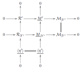
The two relation sheaves lead to two computations of the extension sheaf, summarized in the following commutative diagram of sheaves on $Y^\prime$
with exact rows and columns, where the notation is self-explanatory.
$Y^\prime$
with exact rows and columns, where the notation is self-explanatory.
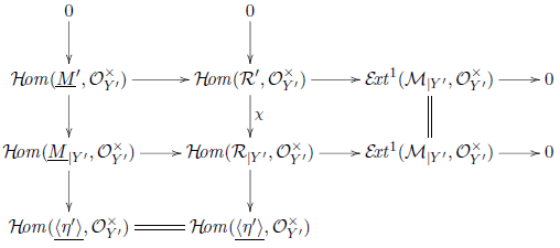
Let $\rho \in \Sigma ^\prime$
be a submaximal cone at which maximal cones
$\rho \in \Sigma ^\prime$
be a submaximal cone at which maximal cones $\sigma _1^\prime , \sigma _2^\prime$
are incident. Denote by
$\sigma _1^\prime , \sigma _2^\prime$
are incident. Denote by $\varphi ^\prime _\rho \colon \mathcal{E} \!{\textit {xt}}^1_c(\mathcal{M}_{|Y^\prime }, \mathcal{O}_{Y^\prime }^\times )\to \mathcal{L}_\rho$
the morphism of sheaves obtained by construction 4.17 on the space
$\varphi ^\prime _\rho \colon \mathcal{E} \!{\textit {xt}}^1_c(\mathcal{M}_{|Y^\prime }, \mathcal{O}_{Y^\prime }^\times )\to \mathcal{L}_\rho$
the morphism of sheaves obtained by construction 4.17 on the space $Y^\prime$
, and by
$Y^\prime$
, and by $\varphi _\rho \colon \mathcal{E} \!{\textit {xt}}^1_c(\mathcal{M}_{|Y^\prime }, \mathcal{O}_{Y^\prime }^\times ) \to \mathcal{L}_\rho$
the morphism of sheaves obtained by Construction 4.17 on the space
$\varphi _\rho \colon \mathcal{E} \!{\textit {xt}}^1_c(\mathcal{M}_{|Y^\prime }, \mathcal{O}_{Y^\prime }^\times ) \to \mathcal{L}_\rho$
the morphism of sheaves obtained by Construction 4.17 on the space $Y$
. We want to show that
$Y$
. We want to show that $\varphi ^\prime = \varphi$
.
$\varphi ^\prime = \varphi$
.
Consider a regular extension $h\in \mathcal{E} \!{\textit {xt}}^1_c(\mathcal{M}_{|Y^\prime }, \mathcal{O}_{Y^\prime }^\times )$
. In order to compute
$h\in \mathcal{E} \!{\textit {xt}}^1_c(\mathcal{M}_{|Y^\prime }, \mathcal{O}_{Y^\prime }^\times )$
. In order to compute $\varphi ^\prime (h)$
, we need to choose a lift in the first row
$\varphi ^\prime (h)$
, we need to choose a lift in the first row
 \begin{align*} (h_{\tau ^\prime })_{\tau ^\prime \in \Sigma ^\prime } \in \mathcal{H}\!{\textit {om}}_c(\mathcal{R}^\prime , \mathcal{O}_{Y^\prime }^\times ) \end{align*}
and follow Construction 4.17 on $Y^\prime$
. Recall that we denote by
$Y^\prime$
. Recall that we denote by $\pi \colon M \to M^\prime$
the natural projection: the cones
$\pi \colon M \to M^\prime$
the natural projection: the cones $\tau ^\prime \in \Sigma ^\prime$
are the projections of the cones of
$\tau ^\prime \in \Sigma ^\prime$
are the projections of the cones of $\Sigma$
that contain
$\Sigma$
that contain $\eta ^\prime$
. The result follows from the observation that
$\eta ^\prime$
. The result follows from the observation that
 \begin{align*} (h_{\tau ^\prime }\circ \pi )_{\eta ^\prime \subset \tau ^\prime \in \Sigma } = \chi \bigl ( (h_{\tau ^\prime })_{\tau ^\prime \in \Sigma ^\prime } \bigr ) \end{align*}
is a lift of $h$
in the second row; that because of Lemma 4.22 it lies in
$h$
in the second row; that because of Lemma 4.22 it lies in $\mathcal{H}\!{\textit {om}}_c(\mathcal{R}_{|Y^\prime }, \mathcal{O}_{Y^\prime }^\times )$
; and that therefore it is good to feed to Construction 4.17 on
$\mathcal{H}\!{\textit {om}}_c(\mathcal{R}_{|Y^\prime }, \mathcal{O}_{Y^\prime }^\times )$
; and that therefore it is good to feed to Construction 4.17 on $Y$
. Unpacking the results leads to
$Y$
. Unpacking the results leads to $\varphi (h)=\varphi ^\prime (h)$
.
$\varphi (h)=\varphi ^\prime (h)$
.
4.7 The morphism
$\varphi$
is injective

Lemma 4.24.
Let $Y$
be a ggtc space. The morphism
$Y$
be a ggtc space. The morphism $\varphi$
of Lemma 4.23 is injective.
$\varphi$
of Lemma 4.23 is injective.
Proof.
In order to show the injectivity of $\varphi$
, we may work on
$\varphi$
, we may work on $Y$
affine satisfying properties (a)–(d) of Setups 4.5 and 4.16.
$Y$
affine satisfying properties (a)–(d) of Setups 4.5 and 4.16.
Assume that we are given two regular tuples $(h_\sigma )_{\sigma \in \Sigma }, (h'_\sigma )_{\sigma \in \Sigma } \in \mathcal{H}\!{\textit {om}} (\mathcal{R}, \mathcal{O}_Y^\times )$
that map to the same section of
$(h_\sigma )_{\sigma \in \Sigma }, (h'_\sigma )_{\sigma \in \Sigma } \in \mathcal{H}\!{\textit {om}} (\mathcal{R}, \mathcal{O}_Y^\times )$
that map to the same section of $\mathcal{LS}^\times _Y$
under
$\mathcal{LS}^\times _Y$
under $\varphi$
.
$\varphi$
.
For $\sigma \in \Sigma$
a maximal cone, the quotient
$\sigma \in \Sigma$
a maximal cone, the quotient $g=(\widetilde {h}_\sigma /\widetilde {h}'_\sigma )_{\sigma \in \Sigma }$
is a homomorphism
$g=(\widetilde {h}_\sigma /\widetilde {h}'_\sigma )_{\sigma \in \Sigma }$
is a homomorphism $g_\sigma \colon M \to \mathcal{O} (\overline U_\sigma )^\times$
. To prove the injectivity of
$g_\sigma \colon M \to \mathcal{O} (\overline U_\sigma )^\times$
. To prove the injectivity of $Y$
, we want to glue these maps to a homomorphism
$Y$
, we want to glue these maps to a homomorphism $g\colon M\to \mathcal{O} (Y)^\times$
, that is,
$g\colon M\to \mathcal{O} (Y)^\times$
, that is, $g \in \Gamma (Y,\mathcal{H}\!{\textit {om}}(\underline {M}, \mathcal{O}_Y^\times ))$
.
$g \in \Gamma (Y,\mathcal{H}\!{\textit {om}}(\underline {M}, \mathcal{O}_Y^\times ))$
.
For gluing along a slab $\rho$
with
$\rho$
with $\sigma _1,\sigma _2$
the maximal cones containing
$\sigma _1,\sigma _2$
the maximal cones containing $\rho$
, since
$\rho$
, since $g_{\sigma _1},g_{\sigma _2}$
already agree on
$g_{\sigma _1},g_{\sigma _2}$
already agree on $\langle \rho \rangle$
, we only need to consider
$\langle \rho \rangle$
, we only need to consider $e_2\in \sigma _2$
at integral distance one from
$e_2\in \sigma _2$
at integral distance one from $\rho$
and we need to have
$\rho$
and we need to have $g_{\sigma _1}(e_2)_{|Y_\rho }=g_{\sigma _2}(e_2)_{|Y_\rho }$
. Assuming
$g_{\sigma _1}(e_2)_{|Y_\rho }=g_{\sigma _2}(e_2)_{|Y_\rho }$
. Assuming $\varphi (h)=\varphi (h')$
gives that
$\varphi (h)=\varphi (h')$
gives that $\varphi \big ((h_\sigma )_{\sigma \in \Sigma }\big )_\rho$
and
$\varphi \big ((h_\sigma )_{\sigma \in \Sigma }\big )_\rho$
and $\varphi \big ((h'_\sigma )_{\sigma \in \Sigma }\big )_\rho$
define the same section of
$\varphi \big ((h'_\sigma )_{\sigma \in \Sigma }\big )_\rho$
define the same section of $\mathcal{L}_\rho$
. In view of the definition (4.6), we then have
$\mathcal{L}_\rho$
. In view of the definition (4.6), we then have
 \begin{align*}\widetilde {h}_{\sigma _1}(e_2)_{|Y_\rho }\otimes \widetilde {h}_{\sigma _2}(-e_2)_{|Y_\rho } = \widetilde {h}'_{\sigma _1}(e_2)_{|Y_\rho }\otimes \widetilde {h}'_{\sigma _2}(-e_2)_{|Y_\rho }.\end{align*}
and rearranging factors yields
 \begin{align} g(e_2)_{|Y_\rho }=g(-e_2)^{-1}_{|Y_\rho } \end{align}
as desired. We can use (4.8) to glue the homomorphisms $g_{\sigma _1}\colon M\to \Gamma (\overline {U}_{\sigma _1} \mathcal{O}_Y^\times )$
and
$g_{\sigma _1}\colon M\to \Gamma (\overline {U}_{\sigma _1} \mathcal{O}_Y^\times )$
and $g_{\sigma _2} \colon M \to \Gamma (\overline {U}_{\sigma _2},\mathcal{O}_Y^\times )$
to a homomorphism
$g_{\sigma _2} \colon M \to \Gamma (\overline {U}_{\sigma _2},\mathcal{O}_Y^\times )$
to a homomorphism $g \colon M\to \Gamma \big ( \overline {U}_{\sigma _1}\cup \overline {U}_{\sigma _2} ,\mathcal{O}_Y^\times \big )$
. Attaching similar gluings along other slabs eventually yields a homomorphism
$g \colon M\to \Gamma \big ( \overline {U}_{\sigma _1}\cup \overline {U}_{\sigma _2} ,\mathcal{O}_Y^\times \big )$
. Attaching similar gluings along other slabs eventually yields a homomorphism $g\colon M\to \Gamma (Y,\mathcal{O}_Y^\times )$
with the property that on each
$g\colon M\to \Gamma (Y,\mathcal{O}_Y^\times )$
with the property that on each $\overline {U}_\tau$
it equals
$\overline {U}_\tau$
it equals $\widetilde {h}_\tau /\widetilde {h}'_\tau$
. It follows from Equation (4.5) that the tuples
$\widetilde {h}_\tau /\widetilde {h}'_\tau$
. It follows from Equation (4.5) that the tuples $(h_\sigma )$
and
$(h_\sigma )$
and $(h'_\sigma )$
project to the same section in
$(h'_\sigma )$
project to the same section in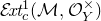 $\mathcal{E} \!{\textit {xt}}_c^1 (\mathcal{M}, \mathcal{O}_Y^\times )$
and hence
$\mathcal{E} \!{\textit {xt}}_c^1 (\mathcal{M}, \mathcal{O}_Y^\times )$
and hence $\varphi$
is injective.
$\varphi$
is injective.
4.8 The morphism
$\varphi$
is surjective

Theorem 4.25.
For every viable ggtc space $Y$
, the morphism
$Y$
, the morphism $\varphi \colon \mathcal{E} \!{\textit {xt}}_c^1 (\mathcal{M}, \mathcal{O}_Y^\times ) \to \mathcal{L}\mathcal{S}^\times _Y$
is bijective.
$\varphi \colon \mathcal{E} \!{\textit {xt}}_c^1 (\mathcal{M}, \mathcal{O}_Y^\times ) \to \mathcal{L}\mathcal{S}^\times _Y$
is bijective.
The statement is local, hence we may work in the following.
Setup 4.26. In the rest of this section we assume that $Y$
satisfies properties (a)–(d) of Setup 4.5 and Setup 4.16 and use freely the notation of Setup 4.5.
$Y$
satisfies properties (a)–(d) of Setup 4.5 and Setup 4.16 and use freely the notation of Setup 4.5.
We begin with some preparations; the proof of the theorem is at the end of the section.
Notation 4.27. For all maximal cones $\sigma \in \Sigma$
we denote by
$\sigma \in \Sigma$
we denote by
 \begin{align*} E_\sigma \in N\otimes _{\mathbb{Z}}\operatorname {\underline {Pic}} (Y_\sigma )=\underline {\operatorname {2-Hom}} (M,\operatorname {\underline {Pic}} Y_\sigma ) \end{align*}
the $2$
-homomorphism such that for all
$2$
-homomorphism such that for all $m\in M$
,
$m\in M$
, $E_\sigma (m)=\mathcal{O}_{Y_\sigma }(-D_\sigma (m))$
.
$E_\sigma (m)=\mathcal{O}_{Y_\sigma }(-D_\sigma (m))$
.
Construction 4.28. Consider two maximal cones $\sigma _1, \sigma _2\in \Sigma$
meeting along a slab
$\sigma _1, \sigma _2\in \Sigma$
meeting along a slab $\rho$
. Denote by
$\rho$
. Denote by $d_{\sigma _1\sigma _2}\in N$
the primitive normal to
$d_{\sigma _1\sigma _2}\in N$
the primitive normal to $\rho$
which evaluates non-negatively on
$\rho$
which evaluates non-negatively on $\sigma _2$
.
$\sigma _2$
.
We construct an isomorphism:
 \begin{align} \psi _{\sigma _1 \sigma _2} \colon \bigl [ E_{\sigma _1|Y_\rho } - d_{\sigma _1\sigma _2}\otimes \mathcal{L}_{\rho } \bigr ] \overset {\cong }{\longrightarrow } E_{\sigma _2|Y_\rho } \quad \text{in $N\otimes _{\mathbb{Z}}\operatorname {\underline {Pic}} Y_\rho $}. \end{align}
Note that this thing unpacks into a collection of isomorphisms, one for each $m\in M$
:
$m\in M$
:
 \begin{align*} \psi _{\sigma _1 \sigma _2} (m) \colon E_{\sigma _1}(m)_{|Y_\rho } \otimes \mathcal{L}_{\rho }^{-d_{\sigma _1\sigma _2}(m)} \overset {\cong }{\longrightarrow } E_{\sigma _2}(m)_{|Y_\rho } \end{align*}
and such that $\psi _{\sigma _1 \sigma _2} (m)$
depends ‘linearly’ on
$\psi _{\sigma _1 \sigma _2} (m)$
depends ‘linearly’ on $m$
.
$m$
.
For $m\in \langle \rho \rangle \cap M$
we have
$m\in \langle \rho \rangle \cap M$
we have $d_{\sigma _1\sigma _2}(m)=0$
: in this case, we define
$d_{\sigma _1\sigma _2}(m)=0$
: in this case, we define $\psi _{\sigma _1 \sigma _2} (m)$
to be the obvious isomorphism obtained by restricting to
$\psi _{\sigma _1 \sigma _2} (m)$
to be the obvious isomorphism obtained by restricting to $Y_\rho$
the restrictable divisors
$Y_\rho$
the restrictable divisors $D_{\sigma _i}(m)$
.
$D_{\sigma _i}(m)$
.
Now fix $e_2\in M$
with
$e_2\in M$
with $d_{\sigma _1\sigma _2} (e_2)=1$
: this gives us the chart
$d_{\sigma _1\sigma _2} (e_2)=1$
: this gives us the chart
 \begin{align*} \lambda (e_2) = {\mathcal{O}_{Y_{\sigma _1}}\bigl (D_{\sigma _1} (-e_2)\bigr )}_{|Y_\rho } \otimes {\mathcal{O}_{Y_{\sigma _2}}\bigl (D_{\sigma _2} (e_2)\bigr )}_{|Y_\rho } \end{align*}
for $\mathcal{L}_\rho$
and we carry out the construction by working in this chart.
$\mathcal{L}_\rho$
and we carry out the construction by working in this chart.
For $m=e_2$
, we define
$m=e_2$
, we define
 \begin{align*} & \psi _{\sigma _1 \sigma _2} (e_2) \colon \bigl ({E_{\sigma _1}}_{|Y_\rho } - d_{\sigma _1\sigma _2}\otimes \lambda (e_2) \bigr )(e_2) \\ &\quad = E_{\sigma _1}(e_e)_{|Y_\rho } \otimes \lambda (e_2)^{-1}\\ &\quad = \mathcal{O}_{Y_{\sigma _1}}(-D_{\sigma _1}(e_2))_{|Y_\rho } \otimes \bigl ({\mathcal{O}_{Y_{\sigma _1}}\bigl (D_{\sigma _1} (-e_2)\bigr )}_{|Y_\rho } \otimes {\mathcal{O}_{Y_{\sigma _2}}\bigl (D_{\sigma _2} (e_2)\bigr )}_{|Y_\rho }\bigr )^{-1}\\ &\quad \overset {\cong }{\longrightarrow } \mathcal{O}_{Y_{\sigma _2}}\bigl (-D_{\sigma _2}(e_2)\bigr ) = E_{\sigma _2|Y_\rho }(e_2). \end{align*}
For general $m\in M$
, there is a unique way to write
$m\in M$
, there is a unique way to write $m=m^\prime +k e_2$
with
$m=m^\prime +k e_2$
with $m^\prime \in \langle \rho \rangle$
and
$m^\prime \in \langle \rho \rangle$
and $k\in \mathbb{Z}$
, and we define
$k\in \mathbb{Z}$
, and we define $\psi _{\sigma _1 \sigma _2} (m)=\psi _{\sigma _1 \sigma _2} (m^\prime ) \otimes \psi _{\sigma _1 \sigma _2} (e_2)^{\otimes k}$
.
$\psi _{\sigma _1 \sigma _2} (m)=\psi _{\sigma _1 \sigma _2} (m^\prime ) \otimes \psi _{\sigma _1 \sigma _2} (e_2)^{\otimes k}$
.
We leave it to the reader to check that all the isomorphisms that one constructs similarly by working in different charts for $\mathcal{L}_\rho$
glue (see the proof of Corollary 3.7 for a model discussion) and that the construction is linear in
$\mathcal{L}_\rho$
glue (see the proof of Corollary 3.7 for a model discussion) and that the construction is linear in $m\in M$
.
$m\in M$
.
Notation 4.29. Assume Setup 4.26 and Notation 4.27.
Fix a nowhere-vanishing section $f_\rho \in \Gamma (Y_\rho ,\mathcal{L}_\rho )$
.
$f_\rho \in \Gamma (Y_\rho ,\mathcal{L}_\rho )$
.
Construction 4.28 provides an isomorphism
 \begin{align} \psi _{\sigma _1 \sigma _2} (f_\rho ) \colon E_{\sigma _1|Y_\rho } \overset {\cong }{\longrightarrow } E_{\sigma _2|Y_\rho } \quad {in} \quad N\otimes \operatorname {\underline {Pic}} (Y_\rho ) \end{align}
given, for all $m\in M$
, as the composition
$m\in M$
, as the composition
 \begin{align*} E_{\sigma _1}(m)_{|Y_\rho }\xrightarrow {(\ ) \times f_\rho ^{-d_{\sigma _1\sigma _2}(m)}} E_{\sigma _1}(m)_{|Y_\rho } \otimes \mathcal{L}_\rho ^{-d_{\sigma _1\sigma _2}(m)} \xrightarrow {\psi _{\sigma _1\sigma _2}(m)} E_{\sigma _2}(m)_{|Y_\rho }. \end{align*}
Definition 4.30. Let $Y$
be a space,
$Y$
be a space, $M$
a lattice,
$M$
a lattice, $N=\operatorname {Hom} (M, \mathbb{Z})$
and
$N=\operatorname {Hom} (M, \mathbb{Z})$
and $E$
an object of the category
$E$
an object of the category $N\otimes _{\mathbb{Z}} \operatorname {\underline {Pic}} (Y)$
.
$N\otimes _{\mathbb{Z}} \operatorname {\underline {Pic}} (Y)$
.
A section upgrade of $E$
is an object
$E$
is an object $\widehat {E}$
of
$\widehat {E}$
of $N\otimes _{\mathbb{Z}} \underline {T} (Y)$
that maps to
$N\otimes _{\mathbb{Z}} \underline {T} (Y)$
that maps to $E$
under the forgetful functor; in other words,
$E$
under the forgetful functor; in other words, $\widehat {E}=(E,e)$
where
$\widehat {E}=(E,e)$
where $e\colon N \otimes \mathcal{O}_Y \to E$
is an isomorphism.
$e\colon N \otimes \mathcal{O}_Y \to E$
is an isomorphism.
Proposition 4.31.
Let $Y$
be an affine viable ggtc space as in Setup 4.26
,
$Y$
be an affine viable ggtc space as in Setup 4.26
, $y\in Y$
a (closed) point, and let
$y\in Y$
a (closed) point, and let $E$
be as in Notation 4.27
.
$E$
be as in Notation 4.27
.
For all $(f_\rho )_{\rho \in T^{[1]}}\in \Gamma (Y,\mathcal{LS}^\times _{Y})$
, possibly after shrinking
$(f_\rho )_{\rho \in T^{[1]}}\in \Gamma (Y,\mathcal{LS}^\times _{Y})$
, possibly after shrinking $Y$
to a smaller affine neighbourhood of
$Y$
to a smaller affine neighbourhood of $y\in Y$
, there exists
$y\in Y$
, there exists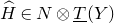 $\widehat {H}\in N \otimes \underline {T}(Y)$
such that:
$\widehat {H}\in N \otimes \underline {T}(Y)$
such that:
-
(1) for every maximal cone
$\sigma$
,
$\widehat {H}_{|Y_\sigma }=(E_\sigma ,e_\sigma )$
is a section upgrade of
$E_\sigma$
; -
(2) for all pairs of maximal cones
$\sigma _1,\sigma _2$
that meet in a slab
$\rho$
, denoting by
$\psi _{\sigma _1\sigma _2}(f_\rho ) \colon E_{\sigma _1|Y_\rho } \overset {\cong }{\longrightarrow } E_{\sigma _2|Y_\rho }$
the isomorphism of Notation 4.29
, we have
\begin{align*} \psi _{\sigma _1\sigma _2}(f_\rho )(e_{\sigma _1|Y_\rho })=e_{\sigma _2|Y_\rho }. \end{align*}

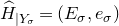




Proof. The boundary complex of a polytope or polyhedral cone is shellable. Recall that this means that there is a shelling, that is an enumeration
 \begin{align*} \sigma _1,\sigma _2, \ldots \end{align*}
of its maximal cones such that for every $k\geqslant 1$
we have that
$k\geqslant 1$
we have that $B_k=\left (\bigcup _{i=1}^k \sigma _i\right )\cap \sigma _{k+1}$
is a pure polyhedral complex of dimension
$B_k=\left (\bigcup _{i=1}^k \sigma _i\right )\cap \sigma _{k+1}$
is a pure polyhedral complex of dimension $\dim M-1$
homeomorphic to either the cone over a ball or the cone over a sphere. Pick a shelling of
$\dim M-1$
homeomorphic to either the cone over a ball or the cone over a sphere. Pick a shelling of $\Sigma$
and fix it for the rest of the proof.
$\Sigma$
and fix it for the rest of the proof.
Choose a section upgrade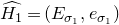 $\widehat {H_1}= (E_{\sigma _1}, e_{\sigma _1})$
. The cones
$\widehat {H_1}= (E_{\sigma _1}, e_{\sigma _1})$
. The cones $\sigma _1$
and
$\sigma _1$
and $\sigma _2$
share exactly one submaximal face
$\sigma _2$
share exactly one submaximal face $\rho$
and Notation 4.29 implies that
$\rho$
and Notation 4.29 implies that
 \begin{align*} \bigl ( E_{\sigma _2|Y_\rho }, \psi _{\sigma _1\sigma _2}(f_\rho )(e_{\sigma _1|Y_\rho })\bigr ) \end{align*}
is a section upgrade of $E_{\sigma _2|Y_\rho }$
. We extend it to a section upgrade
$E_{\sigma _2|Y_\rho }$
. We extend it to a section upgrade $(E_{\sigma _2},e_{\sigma _2})$
of
$(E_{\sigma _2},e_{\sigma _2})$
of $E_{\sigma _2}$
. (This extension might require us to shrink
$E_{\sigma _2}$
. (This extension might require us to shrink $Y$
to a smaller affine neighbourhood of
$Y$
to a smaller affine neighbourhood of $y$
.) After this step, we have produced section upgrades
$y$
.) After this step, we have produced section upgrades $\widehat {E_{\sigma _1}}, \widehat {E_{\sigma _2}}$
of
$\widehat {E_{\sigma _1}}, \widehat {E_{\sigma _2}}$
of ${E}_{\sigma _1},{E}_{\sigma _2}$
that glue along
${E}_{\sigma _1},{E}_{\sigma _2}$
that glue along $Y_\rho$
to give
$Y_\rho$
to give
 \begin{align*} \widehat {H_2} \in N \otimes \underline {T}(Y_{\sigma _1}\cup Y_{\sigma _2}). \end{align*}
Writing $Y_{k-1}=Y_{\sigma _1}\cup \cdots \cup Y_{\sigma _{k-1}}$
, assume by induction that we have constructed:
$Y_{k-1}=Y_{\sigma _1}\cup \cdots \cup Y_{\sigma _{k-1}}$
, assume by induction that we have constructed:
 \begin{align*} \widehat {H_{k-1}} \in N \otimes \underline {T}(Y_{k-1}) \end{align*}
such that parts (1) and (2) hold for all cones $\sigma _i$
and for all pairs of cones
$\sigma _i$
and for all pairs of cones $\sigma _i, \sigma _j$
with
$\sigma _i, \sigma _j$
with $i, j\leqslant k-1$
.
$i, j\leqslant k-1$
.
We construct $\widehat {H_k}$
as follows. In the following, we write
$\widehat {H_k}$
as follows. In the following, we write $\widehat {H_{k-1}}=(H_{k-1},u_{k-1})$
where
$\widehat {H_{k-1}}=(H_{k-1},u_{k-1})$
where $H_{k-1} \in N \otimes \operatorname {\underline {Pic}}(Y_{k-1})$
and
$H_{k-1} \in N \otimes \operatorname {\underline {Pic}}(Y_{k-1})$
and $\widehat {H_{k-1}}$
is a section upgrade. Let
$\widehat {H_{k-1}}$
is a section upgrade. Let $i_1\lt \cdots \lt i_r\leqslant k-1$
be the indices such that
$i_1\lt \cdots \lt i_r\leqslant k-1$
be the indices such that $\sigma _{i_m} \cap \sigma _k =\rho _m\in T^{[1]}$
. We have that
$\sigma _{i_m} \cap \sigma _k =\rho _m\in T^{[1]}$
. We have that
 \begin{align*} Y_{k-1} \cap Y_{\sigma _k} = Y_{\rho _1}\cup \cdots \cup Y_{\rho _r}. \end{align*}
The first step is to construct $H_k\in N \otimes \operatorname {\underline {Pic}} (Y_k)$
by gluing the
$H_k\in N \otimes \operatorname {\underline {Pic}} (Y_k)$
by gluing the $H_{k-1}$
to
$H_{k-1}$
to $E_{\sigma _k}$
by using the isomorphisms
$E_{\sigma _k}$
by using the isomorphisms
 \begin{align*} \psi _{\sigma _{i_m}\sigma _k}(f_{\rho _m}) \colon H_{k-1|Y_{\rho _m}}\overset {\cong }{\longrightarrow } E_{\sigma _k|Y_{\rho _m}}. \end{align*}
Claim. These isomorphisms agree on the joints $Y_\omega$
where two of the
$Y_\omega$
where two of the $Y_\rho$
meet.
$Y_\rho$
meet.
To prove the claim, let us choose such a $\omega$
where two of the
$\omega$
where two of the $\rho$
meet and see what is going on on
$\rho$
meet and see what is going on on $Y_\omega$
. Since
$Y_\omega$
. Since
 \begin{align*} B_{k-1}=\rho _1\cup \cdots \cup \rho _r, \end{align*}
shellability implies that exactly two $\rho$
meet at
$\rho$
meet at $\omega$
, say
$\omega$
, say $\rho _a$
and
$\rho _a$
and $\rho _b$
. We need to show that
$\rho _b$
. We need to show that
 \begin{align*} \psi _{\sigma _{i_a}\sigma _k}(f_{\rho _a}) _{|Y_\omega } \colon H_{k-1|Y_\omega } \to E_{\sigma _k|Y_\omega } \quad \text{equals} \quad \psi _{\sigma _{i_b}\sigma _k}(f_{\rho _b})_{|Y_\omega } \colon H_{k-1|Y_\omega } \to E_{\sigma _k|Y_\omega }. \end{align*}
Shellability implies that there are two increasing sequences of indices:
 \begin{align*} a_1\lt \cdots \lt a_s \leqslant k-1 \quad \text{and} \quad b_1\lt \cdots \lt b_t\leqslant k-1 \quad \text{where} \ a_1=b_1, \; a_s =i_a,\; b_t=i_b \end{align*}
such that
 \begin{align*} \sigma _{a_1}, \sigma _{a_2},\ldots , \sigma _{a_s},\sigma _k, \sigma _{b_t},\ldots , \sigma _{b_2} \end{align*}
is a cyclic enumeration of all the maximal cones of $\Sigma$
incident at
$\Sigma$
incident at $\omega$
. In what follows, we denote by
$\omega$
. In what follows, we denote by $f_{a_i}$
the slab section on
$f_{a_i}$
the slab section on $\sigma _{a_i}\cap \sigma _{a_{i+1}}$
and by
$\sigma _{a_i}\cap \sigma _{a_{i+1}}$
and by $f_{b_i}$
the slab section on
$f_{b_i}$
the slab section on $\sigma _{b_i}\cap \sigma _{b_{i+1}}$
The claim follows from the identity:
$\sigma _{b_i}\cap \sigma _{b_{i+1}}$
The claim follows from the identity:
 \begin{align} \psi _{\sigma _{a_s}\sigma _k}(f_{a_s}) \cdots \psi _{\sigma _{a_1}\sigma _{a_2}}(f_{a_1}) = \psi _{\sigma _{b_t}\sigma _k}(f_{b_t}) \cdots \psi _{\sigma _{b_1}\sigma _{b_2}}(f_{b_1}) \end{align}
on $Y_\omega$
. Evaluating at
$Y_\omega$
. Evaluating at $m\in M$
and using the description in Notation 4.29, identity (4.11) is the joint condition:
$m\in M$
and using the description in Notation 4.29, identity (4.11) is the joint condition:
 \begin{align*} f_{a_s}^{d_{\sigma _{a_s}\sigma _k}(m)} \cdots f_{a_1}^{d_{\sigma _{a_1}\sigma _{a_2}}(m)}= f_{b_t}^{d_{\sigma _{b_t}\sigma _k}(m)} \cdots f_{b_1}^{d_{\sigma _{b_1}\sigma _{b_2}}(m)}. \end{align*}
This proves the claim, and the claim readily implies the result.
Proof of Theorem
4.25. We have shown injectivity in Section 4.7. It suffices to show surjectivity of $\varphi$
at a stalk
$\varphi$
at a stalk $y\in Y$
. Given
$y\in Y$
. Given $s=(f_\rho )_\rho \in \Gamma (Y,\mathcal{LS}^\times _{Y})$
, let
$s=(f_\rho )_\rho \in \Gamma (Y,\mathcal{LS}^\times _{Y})$
, let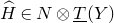 $\widehat {H}\in N\otimes \underline {T}(Y)$
denote the object given by Proposition 4.31. By the construction of
$\widehat {H}\in N\otimes \underline {T}(Y)$
denote the object given by Proposition 4.31. By the construction of $\widehat {H}$
, for every cone
$\widehat {H}$
, for every cone $\tau \in \Sigma _y$
, the restriction of
$\tau \in \Sigma _y$
, the restriction of $\widehat {H}\colon M\to \underline {T}(Y)$
gives a group homomorphism
$\widehat {H}\colon M\to \underline {T}(Y)$
gives a group homomorphism
 \begin{align*} h_{\tau }\colon \langle \tau \rangle \to \mathcal{O} (U_\tau )^\times. \end{align*}
Moreover, the regularity condition from Definition 4.15 is satisfied by the construction of $h$
because
$h$
because $m\in \langle \tau \rangle$
maps to a generator of
$m\in \langle \tau \rangle$
maps to a generator of $\mathcal{O}_{\overline {U}_{\tau }}(-D_\tau (m))$
. The collection of maps
$\mathcal{O}_{\overline {U}_{\tau }}(-D_\tau (m))$
. The collection of maps $h=(h_{\tau })_{\tau \in \Sigma }$
is compatible in the sense that
$h=(h_{\tau })_{\tau \in \Sigma }$
is compatible in the sense that $\rho _\tau ^{\tau '}\circ h_{\tau '}=h_{\tau | {\langle \tau '\rangle }}$
whenever
$\rho _\tau ^{\tau '}\circ h_{\tau '}=h_{\tau | {\langle \tau '\rangle }}$
whenever $\tau '\le \tau$
and so, by (4.4), the collection
$\tau '\le \tau$
and so, by (4.4), the collection $h$
of
$h$
of $h_{\tau }$
constitutes a section of
$h_{\tau }$
constitutes a section of $\mathcal{H}\!{\textit {om}}_c(\mathcal{R},\mathcal{O}_Y^\times )$
and thus it gives a class in
$\mathcal{H}\!{\textit {om}}_c(\mathcal{R},\mathcal{O}_Y^\times )$
and thus it gives a class in $\Gamma (Y,\mathcal{E} \!{\textit {xt}}_c^1 (\mathcal{M}, \mathcal{O}_Y^\times ))$
. By the the key property of
$\Gamma (Y,\mathcal{E} \!{\textit {xt}}_c^1 (\mathcal{M}, \mathcal{O}_Y^\times ))$
. By the the key property of $\widehat {H}$
stated in Proposition 4.31(2), we have
$\widehat {H}$
stated in Proposition 4.31(2), we have $\varphi (h)=s$
.
$\varphi (h)=s$
.
4.9 Local sections of
$\mathcal{E} \!{\textit {xt}}^1_c$
give log structures locally

Proposition 4.32.
Let $Y$
be an affine viable ggtc space as in Setup 4.26
. Consider a regular extension of sheaves of groups
$Y$
be an affine viable ggtc space as in Setup 4.26
. Consider a regular extension of sheaves of groups
 \begin{align*} 0\to \mathcal{O}_Y^\times \to \mathfrak{M} \to \mathcal{M}\to 0.\end{align*}
Then the fiber product $\mathfrak{P}:=\mathfrak{M} \times _{\mathcal{M}} \mathcal{P}$
comes equipped with a monoid homomorphism
$\mathfrak{P}:=\mathfrak{M} \times _{\mathcal{M}} \mathcal{P}$
comes equipped with a monoid homomorphism $\alpha$
to
$\alpha$
to $(\mathcal{O}_Y,\times )$
that yields a compatible log structure on
$(\mathcal{O}_Y,\times )$
that yields a compatible log structure on $Y/k^\dagger$
.
$Y/k^\dagger$
.
Proof.
Consider the relation sheaf sequence (4.3) (this is the same as the first line in (4.12)). By definition $\mathfrak{M}$
is in
$\mathfrak{M}$
is in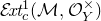 $\mathcal{E} \!{\textit {xt}}_c^1(\mathcal{M}, \mathcal{O}_Y^\times )$
if
$\mathcal{E} \!{\textit {xt}}_c^1(\mathcal{M}, \mathcal{O}_Y^\times )$
if $\mathfrak{M}=\partial (h)$
for a regular
$\mathfrak{M}=\partial (h)$
for a regular $h\in \mathcal{H}\!{\textit {om}}_c (\mathcal{R}, \mathcal{O}_Y^\times )$
, where
$h\in \mathcal{H}\!{\textit {om}}_c (\mathcal{R}, \mathcal{O}_Y^\times )$
, where $\partial$
denotes the boundary map
$\partial$
denotes the boundary map
 \begin{align*} \partial \colon \mathcal{H}\!{\textit {om}}(\mathcal{R},\mathcal{O}_Y^\times )\to \mathcal{E} \!{\textit {xt}}^1 (\mathcal{M}, \mathcal{O}_Y^\times ). \end{align*}
In concrete terms, given $h\colon \mathcal{R}\to \mathcal{O}_Y^\times$
, the extension
$h\colon \mathcal{R}\to \mathcal{O}_Y^\times$
, the extension $\partial h$
is constructed by push out:
$\partial h$
is constructed by push out:

with exact rows and cocartesian squares, where
 \begin{align} \mathfrak{M} = \mathcal{O}_Y^\times \oplus _{\mathcal{R}} \underline {M} = (\mathcal{O}_Y^\times \oplus \underline {M}) / \{(h(m),-m)\,|\,m\in \mathcal{R} \}. \end{align}
Our $\mathfrak{M}$
arises in this way from a regular
$\mathfrak{M}$
arises in this way from a regular $h\in \mathcal{H}\!{\textit {om}}_c (\mathcal{R}, \mathcal{O}_Y^\times )$
. From the concrete description of Lemma 4.11,
$h\in \mathcal{H}\!{\textit {om}}_c (\mathcal{R}, \mathcal{O}_Y^\times )$
. From the concrete description of Lemma 4.11, $h=(h_\tau )_{\tau \in \Sigma }$
where
$h=(h_\tau )_{\tau \in \Sigma }$
where $h_\tau \colon \langle \tau \rangle \to \mathcal{O} (U_\tau )^\times$
is a group homomorphism and, for every
$h_\tau \colon \langle \tau \rangle \to \mathcal{O} (U_\tau )^\times$
is a group homomorphism and, for every $\tau ^\prime \leqslant \tau$
,
$\tau ^\prime \leqslant \tau$
,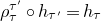 $\rho ^{\tau ^\prime }_\tau \circ h_{\tau ^\prime } = h_\tau$
. Definition 4.15 states that
$\rho ^{\tau ^\prime }_\tau \circ h_{\tau ^\prime } = h_\tau$
. Definition 4.15 states that $h$
is regular if, denoting by
$h$
is regular if, denoting by
 \begin{align*} \iota _\tau \colon \mathcal{O}_Y^\times (U_\tau ) \hookrightarrow \mathcal{K} (\overline {U}_\tau ) \end{align*}
the natural inclusion, we have that for all $\tau \in \Sigma$
and all
$\tau \in \Sigma$
and all $m\in \langle \tau \rangle$
 \begin{align*} \widetilde {h}_\tau (m) = \iota _\tau \circ h_\tau (m) \quad \text{is a generator of} \ \mathcal{O}_{\overline {U}_\tau }\left (-D_\tau (m)\right )\!. \end{align*}
We are now ready to define the log structure $\alpha \colon \mathfrak{P} := \mathfrak{M} \times _{\mathcal{M}} \mathcal{P} \to \mathcal{O}_Y$
. For all
$\alpha \colon \mathfrak{P} := \mathfrak{M} \times _{\mathcal{M}} \mathcal{P} \to \mathcal{O}_Y$
. For all $\tau \in \Sigma$
, we describe
$\tau \in \Sigma$
, we describe
 \begin{align*} \alpha _\tau \colon \mathfrak{P}(U_\tau )=\mathfrak{M} (U_\tau )\times _{M_\tau } P_\tau \to \mathcal{O}(U_\tau ). \end{align*}
For all $\tau \in \Sigma$
, denote by
$\tau \in \Sigma$
, denote by $\pi _\tau \colon M \to M_\tau = M/\langle \tau \rangle$
and by
$\pi _\tau \colon M \to M_\tau = M/\langle \tau \rangle$
and by $\psi _\tau \colon P_\tau \to M_\tau = P_\tau /{\bf 1}_\tau$
the natural projections. An element of
$\psi _\tau \colon P_\tau \to M_\tau = P_\tau /{\bf 1}_\tau$
the natural projections. An element of $\mathfrak{P}(U_\tau )$
is a pair
$\mathfrak{P}(U_\tau )$
is a pair $((\xi , m),p)$
where
$((\xi , m),p)$
where $\xi \in \mathcal{O} (U_\tau )^\times$
,
$\xi \in \mathcal{O} (U_\tau )^\times$
, $m\in M$
,
$m\in M$
, $p\in P_\tau$
, and
$p\in P_\tau$
, and $\pi _\tau (m)=\psi _\tau (p)$
.
$\pi _\tau (m)=\psi _\tau (p)$
.
If $\psi _\tau (p)=0$
, that is,
$\psi _\tau (p)=0$
, that is, $p\in {\bf 1}_\tau + P_\tau$
, then we set
$p\in {\bf 1}_\tau + P_\tau$
, then we set $\alpha _\tau \bigl ( (\xi , m),p \bigr )=0$
.
$\alpha _\tau \bigl ( (\xi , m),p \bigr )=0$
.
Otherwise, there is a smallest cone $\tau \leqslant \tau ^\prime$
such that
$\tau \leqslant \tau ^\prime$
such that $m\in \tau ^\prime$
and
$m\in \tau ^\prime$
and $\pi _\tau (m)=\psi _\tau (p)$
. Note that, in this case,
$\pi _\tau (m)=\psi _\tau (p)$
. Note that, in this case, $\overline {U}_{\tau ^\prime }\cap U_\tau \subset U_\tau$
is a union of irreducible components. In this case, we set
$\overline {U}_{\tau ^\prime }\cap U_\tau \subset U_\tau$
is a union of irreducible components. In this case, we set
 \begin{align*} \alpha _\tau \bigl ( (\xi , m),p \bigr ) = \begin{cases} \widetilde {h}_{\tau ^\prime }(m) \xi _{|\overline {U_{\tau ^\prime }} \cap U_\tau }\; & \text{on $ \overline{U}_{\tau^\prime}\cap U_\tau$;}\\ 0 \; & \text{on $U_\tau\setminus\overline{U}_{\tau^\prime}$.} \end{cases} \end{align*}
The key observation here is that, when $m\in \tau ^\prime$
, the divisor
$m\in \tau ^\prime$
, the divisor $D_{\tau ^\prime } (m) \in \operatorname {Div}^+\overline {U}_{\tau ^\prime }$
is effective; and hence the rational function
$D_{\tau ^\prime } (m) \in \operatorname {Div}^+\overline {U}_{\tau ^\prime }$
is effective; and hence the rational function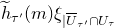 $\widetilde {h}_{\tau ^\prime }(m) \xi _{|\overline {U}_{\tau ^\prime }\cap U_\tau }$
is in fact regular and it vanishes on the boundary, and hence it can be extended by zero to a regular function on all of
$\widetilde {h}_{\tau ^\prime }(m) \xi _{|\overline {U}_{\tau ^\prime }\cap U_\tau }$
is in fact regular and it vanishes on the boundary, and hence it can be extended by zero to a regular function on all of $\overline U_\tau$
.
$\overline U_\tau$
.
It is straightforward to check that $\alpha$
is well-defined; that it is a log structure; and that the global section
$\alpha$
is well-defined; that it is a log structure; and that the global section $\bigl ((1,0),\textbf {1}_{\mathcal{P}}\bigr )$
defines a morphism of log structures
$\bigl ((1,0),\textbf {1}_{\mathcal{P}}\bigr )$
defines a morphism of log structures $Y^\dagger \to (\operatorname {Spec} k)^\dagger$
.
$Y^\dagger \to (\operatorname {Spec} k)^\dagger$
.
4.10 Proof of Theorem 4.3
We want to generalize the constructions in the previous section from the affine situation to the general situation. We begin by rephrasing Proposition 3.11 in [Reference Gross and SiebertGS06] as the following lemma.
Lemma 4.33.
Let $X$
be a reduced Deligne–Mumford stack with two log structures
$X$
be a reduced Deligne–Mumford stack with two log structures $\alpha ,\alpha '\colon \mathfrak{P} \to \mathcal{O}_X$
with identical monoid sheaf. We denote
$\alpha ,\alpha '\colon \mathfrak{P} \to \mathcal{O}_X$
with identical monoid sheaf. We denote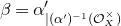 $\beta =\alpha '_{|(\alpha ')^{-1}(\mathcal{O}_X^\times )}$
, so
$\beta =\alpha '_{|(\alpha ')^{-1}(\mathcal{O}_X^\times )}$
, so $\beta$
is an isomorphism onto
$\beta$
is an isomorphism onto $\mathcal{O}_X^\times$
. If
$\mathcal{O}_X^\times$
. If $\alpha \circ \beta ^{-1}\colon \mathcal{O}_X^\times \to \mathcal{O}_X^\times$
is the identity, then
$\alpha \circ \beta ^{-1}\colon \mathcal{O}_X^\times \to \mathcal{O}_X^\times$
is the identity, then $\alpha =\alpha '$
.
$\alpha =\alpha '$
.
Proof.
Consider $\alpha ,\alpha '$
at the generic point
$\alpha ,\alpha '$
at the generic point $\eta$
of a component of
$\eta$
of a component of $X$
,
$X$
, $\alpha _\eta ,\alpha '_\eta \colon \mathfrak{P}_\eta \to \mathcal{O}_{X,\eta }$
. Since
$\alpha _\eta ,\alpha '_\eta \colon \mathfrak{P}_\eta \to \mathcal{O}_{X,\eta }$
. Since $\mathcal{O}_{X,\eta }$
is a field, given
$\mathcal{O}_{X,\eta }$
is a field, given $m\in \mathfrak{P}_\eta$
either
$m\in \mathfrak{P}_\eta$
either $\alpha _\eta (m)=0$
or
$\alpha _\eta (m)=0$
or $\alpha _\eta (m)$
is invertible, similarly for
$\alpha _\eta (m)$
is invertible, similarly for $\alpha '_\eta (m)$
. It follows from the assumptions that
$\alpha '_\eta (m)$
. It follows from the assumptions that $\alpha _\eta =\alpha '_\eta$
. Since
$\alpha _\eta =\alpha '_\eta$
. Since $X$
is reduced, for any open set
$X$
is reduced, for any open set $U$
,
$U$
, $\mathcal{O}_X(U)$
injects into
$\mathcal{O}_X(U)$
injects into $\bigoplus _{\eta \in U} \mathcal{O}_{X,\eta }$
where
$\bigoplus _{\eta \in U} \mathcal{O}_{X,\eta }$
where $\eta$
runs over the generic points of the components of
$\eta$
runs over the generic points of the components of $X$
. The homomorphism
$X$
. The homomorphism $\alpha$
is thus determined by the homomorphisms
$\alpha$
is thus determined by the homomorphisms $\alpha _\eta$
and thus
$\alpha _\eta$
and thus $\alpha =\alpha '$
.
$\alpha =\alpha '$
.
Proof of Theorem
4.3. Let $Y$
be a viable ggtc space.
$Y$
be a viable ggtc space.
Step 1. We construct a morphism of Zariski sheaves of sets on $Y$
:
$Y$
:
 \begin{align} \psi \colon \operatorname {LS}_{k^\dagger } \to \mathcal{E} \!{\textit {xt}}^1_c(\mathcal{M}, \mathcal{O}_Y^\times ). \end{align}
We construct a set-theoretic function $\operatorname {LS}_{k^\dagger }(Y) \to \Gamma \bigl (Y,\mathcal{E} \!{\textit {xt}}_c^1(\mathcal{M}, \mathcal{O}_Y^\times )\bigr )$
that assembles to a sheaf morphism in the input
$\operatorname {LS}_{k^\dagger }(Y) \to \Gamma \bigl (Y,\mathcal{E} \!{\textit {xt}}_c^1(\mathcal{M}, \mathcal{O}_Y^\times )\bigr )$
that assembles to a sheaf morphism in the input $Y$
. Let
$Y$
. Let $\alpha \colon \mathfrak{P}\to \mathcal{O}_Y$
be a compatible log structure. Using
$\alpha \colon \mathfrak{P}\to \mathcal{O}_Y$
be a compatible log structure. Using $\psi \colon \mathfrak{P} \to \mathcal{P}$
from part (1) of Definition 4.2, we can write
$\psi \colon \mathfrak{P} \to \mathcal{P}$
from part (1) of Definition 4.2, we can write $\mathfrak{P}=\mathfrak{M} \times _{\mathcal{M}} \mathcal{P}$
where
$\mathfrak{P}=\mathfrak{M} \times _{\mathcal{M}} \mathcal{P}$
where $\mathfrak{M}=\mathfrak{P}/{\bf 1}_{\mathfrak{P}}$
. All relevant maps being bijective, we identify the projection of
$\mathfrak{M}=\mathfrak{P}/{\bf 1}_{\mathfrak{P}}$
. All relevant maps being bijective, we identify the projection of $\alpha ^{-1}(\mathcal{O}_Y^\times )$
in
$\alpha ^{-1}(\mathcal{O}_Y^\times )$
in $\mathfrak{M}$
with
$\mathfrak{M}$
with $\mathcal{O}_Y^\times$
and obtain an exact sequence as shown as the bottom row in (4.12). We need to show that its extension class lies in
$\mathcal{O}_Y^\times$
and obtain an exact sequence as shown as the bottom row in (4.12). We need to show that its extension class lies in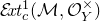 $\mathcal{E} \!{\textit {xt}}_c^1 (\mathcal{M}, \mathcal{O}_Y^\times )$
. This is a local question, so we may assume that
$\mathcal{E} \!{\textit {xt}}_c^1 (\mathcal{M}, \mathcal{O}_Y^\times )$
. This is a local question, so we may assume that $[\mathfrak{M}]=\partial (h)$
for some
$[\mathfrak{M}]=\partial (h)$
for some $h\in \Gamma (Y,\mathcal{H}\!{\textit {om}}(\mathcal{R},\mathcal{O}_Y^\times ))$
so we have a diagram like (4.12). We may also assume that
$h\in \Gamma (Y,\mathcal{H}\!{\textit {om}}(\mathcal{R},\mathcal{O}_Y^\times ))$
so we have a diagram like (4.12). We may also assume that $Y$
is affine as in Setup 4.26. We want to show that
$Y$
is affine as in Setup 4.26. We want to show that $h=(h_\tau )_{\tau \in \Sigma }$
is regular. We need to ‘extract’
$h=(h_\tau )_{\tau \in \Sigma }$
is regular. We need to ‘extract’ $h_\tau (m)$
from the datum of the log structure. Fix
$h_\tau (m)$
from the datum of the log structure. Fix $m\in M$
and let
$m\in M$
and let $\tau \in \Sigma$
be the smallest cone that contains it. There is a unique
$\tau \in \Sigma$
be the smallest cone that contains it. There is a unique $\widehat {m}\in P_\tau \setminus ({\bf 1}_\tau +P_\tau )$
that maps to
$\widehat {m}\in P_\tau \setminus ({\bf 1}_\tau +P_\tau )$
that maps to $m$
under the projection
$m$
under the projection $P_\tau \to M_\tau =P_\tau /{\bf 1}_\tau$
, and it is tautologically the case that, interpreting the pair
$P_\tau \to M_\tau =P_\tau /{\bf 1}_\tau$
, and it is tautologically the case that, interpreting the pair $((1,m),\widehat {m})$
as an element of
$((1,m),\widehat {m})$
as an element of $\mathfrak{P}(U_\tau )=\mathfrak{M}(U_\tau )\times _{M_\tau }P_\tau$
,
$\mathfrak{P}(U_\tau )=\mathfrak{M}(U_\tau )\times _{M_\tau }P_\tau$
,
 \begin{align*} h_\tau (m)=\alpha (\widehat {m}) \in \mathcal{O} (U_\tau ). \end{align*}
By part (b) of Definition 4.2, $\operatorname {div} (h_\tau (m))=D_\tau (m)$
. This holds for all
$\operatorname {div} (h_\tau (m))=D_\tau (m)$
. This holds for all $m\in M$
, hence
$m\in M$
, hence $h$
is regular.
$h$
is regular.
Step 2. The morphism $\psi$
is injective.
$\psi$
is injective.
We need to show that if two compatible log structures give rise to the same extensions, then they are isomorphic as compatible log structures. If the extensions are the same then the two log structures must have isomorphic monoid sheaves compatibly with the respective embeddings of $\mathcal{O}_Y^\times$
and the result follows from Lemma 4.33.
$\mathcal{O}_Y^\times$
and the result follows from Lemma 4.33.
Step 3. The morphism $\psi$
is surjective.
$\psi$
is surjective.
Start from a class in $\Gamma (Y,\mathcal{E} \!{\textit {xt}}_c^1 (\mathcal{M}, \mathcal{O}_Y^\times ))\subset \Gamma (Y,\mathcal{E} \!{\textit {xt}}^1 (\mathcal{M}, \mathcal{O}_Y^\times ))$
. Since
$\Gamma (Y,\mathcal{E} \!{\textit {xt}}_c^1 (\mathcal{M}, \mathcal{O}_Y^\times ))\subset \Gamma (Y,\mathcal{E} \!{\textit {xt}}^1 (\mathcal{M}, \mathcal{O}_Y^\times ))$
. Since $\mathcal{M}$
is supported on the union of slabs, which is of codimension one, we have that
$\mathcal{M}$
is supported on the union of slabs, which is of codimension one, we have that $\mathcal{H}\!{\textit {om}}(\mathcal{M},\mathcal{O}_Y^\times )=0$
. The local-to-global Ext spectral sequence then implies that
$\mathcal{H}\!{\textit {om}}(\mathcal{M},\mathcal{O}_Y^\times )=0$
. The local-to-global Ext spectral sequence then implies that $\Gamma (Y,\mathcal{E} \!{\textit {xt}}^1 (\mathcal{M}, \mathcal{O}_Y^\times ))=\operatorname {Ext}^1(\mathcal{M}, \mathcal{O}_Y^\times )$
, so we obtain a sheaf
$\Gamma (Y,\mathcal{E} \!{\textit {xt}}^1 (\mathcal{M}, \mathcal{O}_Y^\times ))=\operatorname {Ext}^1(\mathcal{M}, \mathcal{O}_Y^\times )$
, so we obtain a sheaf $\mathfrak{M}$
that sits in the middle of an exact sequence as in Proposition 4.32. We then produce the monoid sheaf
$\mathfrak{M}$
that sits in the middle of an exact sequence as in Proposition 4.32. We then produce the monoid sheaf $\mathfrak{P} := \mathfrak{M} \times _{\mathcal{M}} \mathcal{P}$
which locally comes with a homomorphism to
$\mathfrak{P} := \mathfrak{M} \times _{\mathcal{M}} \mathcal{P}$
which locally comes with a homomorphism to $(\mathcal{O}_Y,\cdot )$
by Proposition 4.32. These local maps glue to a global one by the uniqueness of these maps according to Lemma 4.33.
$(\mathcal{O}_Y,\cdot )$
by Proposition 4.32. These local maps glue to a global one by the uniqueness of these maps according to Lemma 4.33.
Step 4. End of proof of Theorem 4.3.
We define the composition
 \begin{align} r=\varphi \circ \psi \colon \operatorname {LS}_{k^\dagger } \to \mathcal{LS}_Y^\times \end{align}
of $\psi$
from (4.14) with the bijection
$\psi$
from (4.14) with the bijection $\varphi$
from Theorem 4.25.
$\varphi$
from Theorem 4.25.
5. Examples
5.1 Two components
In this section, $Y$
consists of two smooth components
$Y$
consists of two smooth components $Y_1, Y_2$
meeting along a smooth irreducible divisor
$Y_1, Y_2$
meeting along a smooth irreducible divisor $D\subset Y_{i}$
(
$D\subset Y_{i}$
( $i=1,2$
) all defined over
$i=1,2$
) all defined over $k$
. First, we describe a sheaf of monoids
$k$
. First, we describe a sheaf of monoids $\mathcal{P}$
on
$\mathcal{P}$
on $Y$
that allows us to equip
$Y$
that allows us to equip $Y$
with the structure of a ggtc space; then, we study the log structures
$Y$
with the structure of a ggtc space; then, we study the log structures $\mathfrak{P}$
on
$\mathfrak{P}$
on $Y$
that have ghost sheaf
$Y$
that have ghost sheaf $\mathcal{P}$
, and finally we see how to keep track of a morphism to the standard log point
$\mathcal{P}$
, and finally we see how to keep track of a morphism to the standard log point $\operatorname {Spec} k ^\dagger$
. This is the most elementary example of the theory but it is nevertheless quite rich and it is well worth it to invest the time necessary to understand it completely.
$\operatorname {Spec} k ^\dagger$
. This is the most elementary example of the theory but it is nevertheless quite rich and it is well worth it to invest the time necessary to understand it completely.
The simplest source of examples of log structures on $Y$
are embeddings
$Y$
are embeddings $i\colon Y \hookrightarrow X$
into a smooth scheme
$i\colon Y \hookrightarrow X$
into a smooth scheme $X$
. More generally, we can look at an embedding where locally analytically (or étale locally)
$X$
. More generally, we can look at an embedding where locally analytically (or étale locally) $Y=(t=0) \subset X$
where
$Y=(t=0) \subset X$
where $X=(xy+t^r=0)\subset \mathbb{A}^3_{x,y,t}\times \mathbb{A}^m$
for
$X=(xy+t^r=0)\subset \mathbb{A}^3_{x,y,t}\times \mathbb{A}^m$
for $m=\dim D$
.
$m=\dim D$
.
Given such an embedding one can form the divisorial log structure $\mathfrak{P}_{X,Y}=\mathcal{O}_X\cap \mathcal{O}_{X\setminus Y}^\times$
on
$\mathfrak{P}_{X,Y}=\mathcal{O}_X\cap \mathcal{O}_{X\setminus Y}^\times$
on $X$
, and the log structure
$X$
, and the log structure $\mathfrak{P}_Y=i^\star \mathfrak{P}_{X,Y}$
on
$\mathfrak{P}_Y=i^\star \mathfrak{P}_{X,Y}$
on $Y$
. In the following we make log structures on
$Y$
. In the following we make log structures on $Y$
of this étale local type without reference to an embedding. Fix an integer
$Y$
of this étale local type without reference to an embedding. Fix an integer $r\gt 0$
, consider the sublattice
$r\gt 0$
, consider the sublattice
 \begin{align*} M=\{(n_1,n_2)\mid n_1 \equiv n_2 (\text{mod}\ {r})\}\subset \mathbb{Z}^2, \end{align*}
illustrated in Figure 6, and let $P=\langle e_1,e_2\rangle _+\cap M$
be the monoid of lattice points in the positive quadrant. This monoid is generated by
$P=\langle e_1,e_2\rangle _+\cap M$
be the monoid of lattice points in the positive quadrant. This monoid is generated by $(r,0)$
,
$(r,0)$
, $(0,r)$
and
$(0,r)$
and $(1,1)$
with the obvious relation. We use
$(1,1)$
with the obvious relation. We use $P$
to define a sheaf of monoids on
$P$
to define a sheaf of monoids on $Y$
as follows. For a connected Zariski open subset
$Y$
as follows. For a connected Zariski open subset $U\subset Y$
, we set
$U\subset Y$
, we set
 \begin{align*} \mathcal{P} (U) = \begin{cases} P \; & \text{if $U\cap D\neq \emptyset $,}\\ P/\langle re_2 \rangle \cong \mathbb{N} \; & \text{if $U\subset Y\setminus Y_2$,} \\ P/\langle re_1 \rangle \cong \mathbb{N} \; & \text{if $U\subset Y\setminus Y_1$.} \\ \end{cases} \end{align*}
Now $Y$
is a ggtc space with ghost sheaf
$Y$
is a ggtc space with ghost sheaf $\mathcal{P}$
in a natural way: if locally at the generic point
$\mathcal{P}$
in a natural way: if locally at the generic point $\eta \in D$
we have
$\eta \in D$
we have $Y=(xy=0)$
where say
$Y=(xy=0)$
where say $Y_1=(y=0)$
and
$Y_1=(y=0)$
and $Y_2=(x=0)$
, then we have
$Y_2=(x=0)$
, then we have $k[P]=k[x,y,t]/(xy+t^r)$
. In what follows, it is crucial to understand that
$k[P]=k[x,y,t]/(xy+t^r)$
. In what follows, it is crucial to understand that $x\in k[P]$
vanishes with multiplicity
$x\in k[P]$
vanishes with multiplicity $r$
along
$r$
along $Y_2$
.
$Y_2$
.
The sublattice $M\subset \mathbb{Z}^2$
for
$M\subset \mathbb{Z}^2$
for $r=3$
.
$r=3$
.
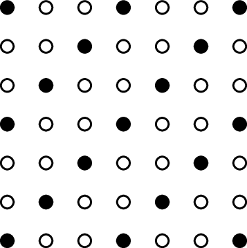
Proposition 5.1.
Let $r\gt 0$
and
$r\gt 0$
and $Y=Y_1+Y_2$
a toroidal crossing space as just described. To give a log structure
$Y=Y_1+Y_2$
a toroidal crossing space as just described. To give a log structure $\mathfrak{P}$
on
$\mathfrak{P}$
on $Y$
is equivalent to giving line bundles
$Y$
is equivalent to giving line bundles $\mathcal{L}_1, \mathcal{L}_2,\mathcal{L}$
on
$\mathcal{L}_1, \mathcal{L}_2,\mathcal{L}$
on $Y$
, homomorphisms
$Y$
, homomorphisms $\alpha _1\colon \mathcal{L}_1\to \mathcal{O}_Y$
,
$\alpha _1\colon \mathcal{L}_1\to \mathcal{O}_Y$
, $\alpha _2\colon \mathcal{L}_2\to \mathcal{O}_Y$
such that
$\alpha _2\colon \mathcal{L}_2\to \mathcal{O}_Y$
such that
 \begin{align} \alpha _{1|Y_2}\colon \mathcal{L}_{1|Y_2}\overset {\cong }{\longrightarrow }\mathcal{O}_{Y_2}(-D)\subset \mathcal{O}_{Y_2} & \quad \text{and} \quad \alpha _{1|Y_1} = 0, \end{align}
 \begin{align} \alpha _{2|Y_1}\colon \mathcal{L}_{2|Y_1}\overset {\cong }{\longrightarrow }\mathcal{O}_{Y_1}(-D)\subset \mathcal{O}_{Y_1} & \quad \text{and} \quad \alpha _{2|Y_2} = 0; \end{align}
and an identification $s\colon \mathcal{L}^{\otimes r} \overset {\cong }{\longrightarrow } \mathcal{L}_1\otimes \mathcal{L}_2$
.
$s\colon \mathcal{L}^{\otimes r} \overset {\cong }{\longrightarrow } \mathcal{L}_1\otimes \mathcal{L}_2$
.
Sketch of proof.
We construct a log structure from the data spelled out in the proposition. First of all, for $p=n_1(r,0)+q(1,1)\in P$
, that is,
$p=n_1(r,0)+q(1,1)\in P$
, that is, $q\geqslant 0,n_1\in \mathbb{Z}$
satisfying
$q\geqslant 0,n_1\in \mathbb{Z}$
satisfying $n_1+ {q}/{r} \geqslant 0$
, write
$n_1+ {q}/{r} \geqslant 0$
, write
 \begin{align*} \mathcal{L}^p = \mathcal{L}_1^{\otimes n_1} \otimes \mathcal{L}^{\otimes q}. \end{align*}
Note how this choice singles out a $2$
-homomorphism from the monoid
$2$
-homomorphism from the monoid $P$
, viewed as a category, to the
$P$
, viewed as a category, to the $2$
-group
$2$
-group $\operatorname {\underline {Pic}} Y$
. The log structure is the sheaf of monoids:
$\operatorname {\underline {Pic}} Y$
. The log structure is the sheaf of monoids:
 \begin{align*} \mathfrak{P} (U) = \begin{cases} \coprod _{p\in P} \mathcal{L}^p (U)^\times \; & \text{if $U\cap D\neq \emptyset$,}\\ \coprod _{q\in \mathbb{N}} \mathcal{L}^{\otimes q} (U )^\times \; & \text{if $U\subset Y\setminus Y_2$,} \\ \coprod _{q\in \mathbb{N}} \mathcal{L}^{\otimes q} (U )^\times \; & \text{if $U\subset Y\setminus Y_1$,} \end{cases} \end{align*}
together with the obvious homomorphism $\alpha \colon \mathfrak{P} \to \mathcal{O}_Y$
.
$\alpha \colon \mathfrak{P} \to \mathcal{O}_Y$
.
We want to understand isomorphism classes of log structures on $Y$
over
$Y$
over $\operatorname {Spec} k^\dagger$
, where we map
$\operatorname {Spec} k^\dagger$
, where we map $\mathbb{N}\to P$
by taking
$\mathbb{N}\to P$
by taking $1$
to
$1$
to ${\bf 1}=(1,1)$
: it is surprising to see that this set has a simpler description as follows.
${\bf 1}=(1,1)$
: it is surprising to see that this set has a simpler description as follows.
Proposition 5.2.
Let $Y=Y_1+Y_2$
be a toroidal crossing space as above. The set of isomorphism classes of log structures on
$Y=Y_1+Y_2$
be a toroidal crossing space as above. The set of isomorphism classes of log structures on $Y$
over
$Y$
over $\operatorname {Spec} k^\dagger$
is the set of nowhere-vanishing sections of the sheaf
$\operatorname {Spec} k^\dagger$
is the set of nowhere-vanishing sections of the sheaf
 \begin{align*} \mathcal{L}_D=\left (N_{Y_1} D\right )\otimes \left (N_{Y_2}D\right)\!.\end{align*}
Sketch of proof.
Suppose given a log structure $\mathfrak{P}$
on
$\mathfrak{P}$
on $Y$
, making it into a log scheme
$Y$
, making it into a log scheme $Y^\dagger$
. In the notation of the previous proposition, a morphism
$Y^\dagger$
. In the notation of the previous proposition, a morphism $Y^\dagger \to \operatorname {Spec} k^\dagger$
is precisely the datum of a nowhere-vanishing global section
$Y^\dagger \to \operatorname {Spec} k^\dagger$
is precisely the datum of a nowhere-vanishing global section $\sigma _0 \in H^0(Y,\mathcal{L})$
. This also gives a section
$\sigma _0 \in H^0(Y,\mathcal{L})$
. This also gives a section $\sigma =\sigma _0^r \in H^0(Y, \mathcal{L}^{\otimes r})$
that we pass through the isomorphism
$\sigma =\sigma _0^r \in H^0(Y, \mathcal{L}^{\otimes r})$
that we pass through the isomorphism $s$
to trivialize the line bundle
$s$
to trivialize the line bundle $\mathcal{L}_1\otimes \mathcal{L}_2$
. Thus, for example, we have
$\mathcal{L}_1\otimes \mathcal{L}_2$
. Thus, for example, we have
 \begin{align*} {\mathcal{L}_1}_{|Y_2} & =\mathcal{O}_{Y_2}(-D),\\ {\mathcal{L}_1}_{|Y_1} & \stackrel {s(\sigma )}{=}{\mathcal{L}_2^\star }_{|Y_1}=\mathcal{O}_{Y_1}(D).\end{align*}
Thus, $\mathcal{L}_1$
is glued together from an isomorphism
$\mathcal{L}_1$
is glued together from an isomorphism
 \begin{align*} f\colon {\mathcal{O}_{Y_2}(-D)}_{|D}=N_{Y_2}^\star D \overset {\cong }{\longrightarrow } N_{Y_1} D ={\mathcal{O}_{Y_1}(D)}_{|D} \end{align*}
or, equivalently, a nowhere-vanishing section of
 \begin{align*} \mathcal{LS}_Y = (N_{Y_1} D) \otimes (N_{Y_2} D). \end{align*}
In particular. in order for the log structure over $\operatorname {Spec} k^\dagger$
to even exist, one must have that
$\operatorname {Spec} k^\dagger$
to even exist, one must have that $\mathcal{LS}_Y$
is a trivial line bundle.
$\mathcal{LS}_Y$
is a trivial line bundle.
Remark 5.3.
-
(1) Perhaps surprisingly, the sheaf
$\mathcal{LS}_Y=\mathcal{L}_D$
in the example, and thus the fact of the existence of a compatible log structure over the standard log point, does not depend on
$r$
. -
(2) It is a matter of convention whether
$\mathcal{LS}_Y=N_{Y_1}D\otimes N_{Y_2}D$
or its dual. Our convention is motivated by the fact that we want
$\mathcal{LS}_Y$
to have lots of sections when
$N_{Y_1}D\otimes N_{Y_2}D$
has lots of sections. These sections of
$\mathcal{LS}_Y$
are useful even when they vanish somewhere and we think of them as giving ‘singular’ log structures, as justified in Definition 5.4. Furthermore, sections with vanishing loci in
$\mathcal{LS}_Y$
may arise from restrictions of divisorial log structures of a pair
$(X,Y)$
to the divisor
$Y$
. The convention also fits with the existence of an isomorphism
$\mathcal{LS}_Y\cong \mathcal{T}^1_Y$
in the normal crossing case [Reference Felten, Filip and RuddatFFR21].







Definition 5.4. We adopt the following language from the Gross–Siebert program initiated in [Reference Gross and SiebertGS06].
-
(i) We say that a section of
$\mathcal{LS}_Y$
whose vanishing locus is a divisor
$Z\subset D$
is a log structure on
$Y$
singular along
$Z$
. A priori, the log structure is only defined on
$Y\setminus Z$
. A log structure on all of
$Y$
can be produced by taking the direct image of the log structure on
$Y\setminus Z$
. This direct image log structure fails to be coherent along
$Z$
. Failure of coherence prevents the log scheme from satisfying the formal log smoothness lifting criterion as we explain in the simplest example below, so calling the log structure singular along
$Z$
is justified. With regards to part (2) of the previous remark we view a log structure from a section of
$\mathcal{LS}_Y$
on an open set that extends with poles in its complement as pathological. -
(ii) In the above example, the sheaf
$\mathcal{LS}_Y$
was a line bundle on
$D$
, identical with the unique slab bundle. More generally, as in Definition 3.9,
$\mathcal{LS}_Y$
is defined as a subsheaf of the direct sum of slab bundles cut out by the joint condition. We call a section
$f_\rho$
of a slab bundle
$\mathcal{L}_\rho$
a slab section, typically studied in a local trivialization of the bundle where we may also call it a slab function.
-
(iii) Each slab bundle comes with a positive integer like the integer
$r$
above which appears in its frame from the relation
$xy=z^r$
. We refer to this integer as the kink of the slab.


5.2 The easiest singular log structure
It pays off to study the easiest singular log structure that there is and understand it completely.
Consider $\mathbb{A}^3$
with coordinates
$\mathbb{A}^3$
with coordinates $x,y,u$
; we take
$x,y,u$
; we take $X$
to be the surface
$X$
to be the surface
 \begin{align*} X= \bigl (xy=0\bigr ) \subset \mathbb{A}^3. \end{align*}
Note that $X$
consists of two components
$X$
consists of two components
 \begin{align*} X_1=\mathbb{A}^2_{x,u}= \left (y=0\right )\!,\quad X_2=\mathbb{A}^2_{y,u}= \left (x=0\right )\!. \end{align*}
Let us write $S=X_1\cap X_2=\mathbb{A}^1_u$
. The slab bundle for the slab
$S=X_1\cap X_2=\mathbb{A}^1_u$
. The slab bundle for the slab $S$
is trivial. We endow
$S$
is trivial. We endow $X$
with the log structure over
$X$
with the log structure over $k^\dagger$
given by the slab function
$k^\dagger$
given by the slab function
 \begin{align*} f_\rho (u) =u \end{align*}
on $S$
. Denoting the origin by
$S$
. Denoting the origin by ${\bf 0}$
, we set
${\bf 0}$
, we set $Z=\{{\bf 0}\}\subset S$
, write
$Z=\{{\bf 0}\}\subset S$
, write $U=X\setminus Z$
,
$U=X\setminus Z$
, $S^\star =S\setminus Z$
and denote by
$S^\star =S\setminus Z$
and denote by $j\colon U \to X$
the natural inclusion. Since
$j\colon U \to X$
the natural inclusion. Since $f_\rho$
vanishes outside
$f_\rho$
vanishes outside $U$
, the log structure only exists on
$U$
, the log structure only exists on $U$
and we denote its sheaf of monoids by
$U$
and we denote its sheaf of monoids by $\mathfrak{P}_U$
. To obtain a log structure on
$\mathfrak{P}_U$
. To obtain a log structure on $X$
we use
$X$
we use $\mathfrak{M}_X=j_\star \mathfrak{P}_U$
and arrive at a log morphism
$\mathfrak{M}_X=j_\star \mathfrak{P}_U$
and arrive at a log morphism $f\colon X^\dagger \to \operatorname {Spec} k^\dagger$
which is not formally log smooth at
$f\colon X^\dagger \to \operatorname {Spec} k^\dagger$
which is not formally log smooth at $Z$
. This can be seen as follows. One first verifies that the stalk
$Z$
. This can be seen as follows. One first verifies that the stalk $\alpha _{{\bf 0}}\colon \mathfrak{M}_{X,{\bf 0}}\to \mathcal{O}_{X,{\bf 0}}$
agrees with the stalk of log structure obtained as pull-back from
$\alpha _{{\bf 0}}\colon \mathfrak{M}_{X,{\bf 0}}\to \mathcal{O}_{X,{\bf 0}}$
agrees with the stalk of log structure obtained as pull-back from $\operatorname {Spec} k^\dagger$
. That is, the log morphism
$\operatorname {Spec} k^\dagger$
. That is, the log morphism $f$
is strict at
$f$
is strict at ${\bf 0}$
. Since the underlying morphism is not formally smooth, there is a test diagram with a square zero extension as in the definition of formal smoothness that has no diagonal map. Enrich this diagram with pull-back log structures from
${\bf 0}$
. Since the underlying morphism is not formally smooth, there is a test diagram with a square zero extension as in the definition of formal smoothness that has no diagonal map. Enrich this diagram with pull-back log structures from $\operatorname {Spec} k^\dagger$
and it also will not have a diagonal map, so formal log smoothness fails at
$\operatorname {Spec} k^\dagger$
and it also will not have a diagonal map, so formal log smoothness fails at ${\bf 0}$
. On the other hand, formal log smoothness works over
${\bf 0}$
. On the other hand, formal log smoothness works over $U$
which we leave as an exercise.
$U$
which we leave as an exercise.
As explained in Section 5.1, the log structure on $U$
is determined by line bundles
$U$
is determined by line bundles
 \begin{align*} \mathcal{L}_{1\, U}, \quad \mathcal{L}_{2\,U}, \quad \mathcal{L}_U \end{align*}
on $U$
, and homomorphisms
$U$
, and homomorphisms $\alpha _i\colon \mathcal{L}_{i\,U}\to \mathcal{O}$
satisfying the conditions in Proposition 5.1, and
$\alpha _i\colon \mathcal{L}_{i\,U}\to \mathcal{O}$
satisfying the conditions in Proposition 5.1, and $s\colon \mathcal{L}_U \overset {\cong }{\longrightarrow } \mathcal{L}_{1\,U} \otimes \mathcal{L}_{2\,U}$
. Following the recipe in the proof of Proposition 5.2, the line bundle
$s\colon \mathcal{L}_U \overset {\cong }{\longrightarrow } \mathcal{L}_{1\,U} \otimes \mathcal{L}_{2\,U}$
. Following the recipe in the proof of Proposition 5.2, the line bundle $\mathcal{L}_{2 U}$
, for example, is obtained by assembling the line bundles
$\mathcal{L}_{2 U}$
, for example, is obtained by assembling the line bundles $\mathcal{O}_{U_1}$
on
$\mathcal{O}_{U_1}$
on $U_1$
and
$U_1$
and $\mathcal{O}_{U_2}$
on
$\mathcal{O}_{U_2}$
on $U_2$
via the isomorphism
$U_2$
via the isomorphism
 \begin{align*} \text{multiplication by $u$}: \mathcal{O}_{U_1|S^\star } =\mathcal{O}_{S^\star } \overset {\cong }{\longrightarrow } \mathcal{O}_{S^\star } = \mathcal{O}_{U_2|S^\star }. \end{align*}
It follows from this that $\mathcal{L}_2=j_\star \mathcal{L}_{2\, U}$
is the reflexive sheaf on
$\mathcal{L}_2=j_\star \mathcal{L}_{2\, U}$
is the reflexive sheaf on $X$
associated to the
$X$
associated to the $k[x,y,u]/_{(xy)}$
-module
$k[x,y,u]/_{(xy)}$
-module
 \begin{align*} M_1=\Gamma \left (\mathcal{L}_{1\, U} ,U\right ) =\langle e_1=(1,u),\, e_2=(0,y)\mid ye_1=ue_2, xe_2\rangle. \end{align*}
Note for example that $(x,0)=xe_1$
,
$(x,0)=xe_1$
, $(1,u+y)=e_1+e_2$
, etc. Although
$(1,u+y)=e_1+e_2$
, etc. Although $\mathcal{L}_2$
is not a line bundle on
$\mathcal{L}_2$
is not a line bundle on $X$
, the restrictions
$X$
, the restrictions $\mathcal{L}_{2|X_1}$
and
$\mathcal{L}_{2|X_1}$
and $\mathcal{L}_{2|X_2}$
are line bundles.
$\mathcal{L}_{2|X_2}$
are line bundles.
The homomorphism $\alpha \colon M \to k[x,y]/_{(xy)}$
is defined as
$\alpha \colon M \to k[x,y]/_{(xy)}$
is defined as
 \begin{align*} \alpha (1,u)=x,\quad \alpha (0,y)=0, \end{align*}
that is,
 \begin{align*} \alpha \colon \mathcal{L}_{2|X_1}\overset {\cong }{\longrightarrow }\mathcal{O}_{X_1}(-S),\quad \alpha \colon \mathcal{L}_{2|X_2} =0 \end{align*}
Naturally $\mathcal{L}_1=\mathcal{L}_2^\vee$
and
$\mathcal{L}_1=\mathcal{L}_2^\vee$
and $\mathcal{L} =\mathcal{O}_X=\mathcal{L}_1[\otimes ] \mathcal{L}_2$
where
$\mathcal{L} =\mathcal{O}_X=\mathcal{L}_1[\otimes ] \mathcal{L}_2$
where $[\otimes ]$
refers to the reflexive tensor product.Footnote
23
$[\otimes ]$
refers to the reflexive tensor product.Footnote
23
Take $Y_1=X_1$
, let
$Y_1=X_1$
, let $Y_2\to X_2$
be the blow up of
$Y_2\to X_2$
be the blow up of $X_2$
at the origin, assemble
$X_2$
at the origin, assemble $Y_1$
and
$Y_1$
and $Y_2$
to obtain
$Y_2$
to obtain $Y$
and denote by
$Y$
and denote by $f\colon Y\to X$
the proper birational map; the exceptional set is
$f\colon Y\to X$
the proper birational map; the exceptional set is $E\cong \mathbb{P}^1\subset Y$
and
$E\cong \mathbb{P}^1\subset Y$
and $f_{|Y\setminus E}\colon Y\setminus E \to X\setminus Z$
is an isomorphism. Then
$f_{|Y\setminus E}\colon Y\setminus E \to X\setminus Z$
is an isomorphism. Then
 \begin{align*} \mathcal{LS}_Y=f^{\star} \left (\mathcal{LS}_X(-Z)\right )\!. \end{align*}
There is a unique log structure on $Y$
over
$Y$
over $k^\dagger$
that agrees on
$k^\dagger$
that agrees on
 \begin{align*} Y\setminus E \overset {f}{=} X\setminus Z \end{align*}
with the given one and is log smooth over $k^\dagger$
because the section
$k^\dagger$
because the section $f_\rho =u\in \Gamma (S^\star ,\mathcal{LS}_Y)$
extends as a nowhere-vanishing section of
$f_\rho =u\in \Gamma (S^\star ,\mathcal{LS}_Y)$
extends as a nowhere-vanishing section of $\mathcal{LS}_Y$
on
$\mathcal{LS}_Y$
on $S$
.
$S$
.
The moment polyhedral complex of the surface $X$
.
$X$
.
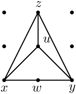
Figure 7. Long description
The diagram depicts a polyhedral complex on a surface. It features a triangular structure with vertices labeled as x, y, z, w, and u. The vertices are connected by edges forming a triangular shape with an additional internal vertex labeled u. The diagram illustrates the relationships and connections between these vertices within the polyhedral complex.
5.3 A reducible quartic del Pezzo surface
5.3.1 Description of the surface and log structure.
We start from $X$
the toroidal crossing surface given as the union of three toric surfaces as in the moment polygonal complex pictured in Figure 7. From the picture we see that
$X$
the toroidal crossing surface given as the union of three toric surfaces as in the moment polygonal complex pictured in Figure 7. From the picture we see that $X$
is naturally embedded in
$X$
is naturally embedded in $\mathbb{P}^4$
and given by equations:
$\mathbb{P}^4$
and given by equations:
 \begin{align*} X= \left \{ \begin{aligned} xy-w^2 & =0 \\ zw & = 0 \end{aligned} \right. \end{align*}
in homogeneous coordinates $x:y:z:u:w$
. The three components of
$x:y:z:u:w$
. The three components of $X$
are
$X$
are
 \begin{align*} X_1= (z=xy-w^2=0 ); \quad X_2= (w=x=0 ); \quad \text{and}\quad X_3= (w=y=0 ). \end{align*}
The obvious and, essentially, unique polarization (see Lemma 2.3) has kink $\kappa=1$
along the
$\kappa=1$
along the $x$
and
$x$
and $y$
axes and
$y$
axes and $\kappa=2$
along the
$\kappa=2$
along the $z$
-axis.Footnote
24
The datum of a log structure on
$z$
-axis.Footnote
24
The datum of a log structure on $X$
over
$X$
over $k^\dagger$
consists of slab sections:
$k^\dagger$
consists of slab sections:
 \begin{align*} f_{\rho _x} & = a_0+a_1x+a_2x^2 \\ f_{\rho _y} & = b_0+b_1y+b_2y^2 \\ f_{\rho _z} & =c_0 + c_1z+c_2z^2+c_3z^3+c_4z^4 \end{align*}
(in the affine patch $u=1$
) and the joint condition at the origin states that
$u=1$
) and the joint condition at the origin states that
 \begin{align} a_0=b_0\quad \hbox{and}\quad c_0=a_0^2. \end{align}
From now on we fix general slab sections and denote by $X^\dagger /k^\dagger$
the surface
$X^\dagger /k^\dagger$
the surface $X$
equipped with the log structure and structure morphism
$X$
equipped with the log structure and structure morphism $X^\dagger \to \operatorname {Spec} k^\dagger$
given by these functions.
$X^\dagger \to \operatorname {Spec} k^\dagger$
given by these functions.
The morphism is not log smooth: it is singular along the union of points $Z\subset X$
where the slab sections vanish. For generic coefficients, we find
$Z\subset X$
where the slab sections vanish. For generic coefficients, we find $8$
such points. We next show how these log structures arise naturally when we deform the surface
$8$
such points. We next show how these log structures arise naturally when we deform the surface $X$
.
$X$
.
5.3.2 Log deformations of
$X^\dagger /k^\dagger$
.

Consider the family of surfaces over $\mathbb{A}^1$
with coordinate
$\mathbb{A}^1$
with coordinate $t$
given by the equations
$t$
given by the equations
 \begin{align} \mathfrak{X} = \left \{ \begin{aligned} xy-w^2 & =ts_1wu+t^2\big(c_2u^2+c_3uz+c_4z^2\big)\\ zw & = t\big(s_0u^2+a_1xu+a_2x^2+b_1yu+b_2y^2\big) \end{aligned} \right. \end{align}
in $\mathbb{P}^4 \times \mathbb{A}^{1}$
. Note the following.
$\mathbb{P}^4 \times \mathbb{A}^{1}$
. Note the following.
-
(1) Together with the projection
$\pi \colon \mathfrak{X} \to \mathbb{A}^1$
the equations represent a flat deformation, in fact, a smoothing, of the surface
$X=\mathfrak{X}_0$
. The general fiber is a del Pezzo surface of degree
$4$
: a smooth intersection of two quadrics in
$\mathbb{P}^4$
. -
(2) Denote by
$i \colon X \hookrightarrow \mathfrak{X}$
the natural inclusion. The total space
$\mathfrak{X}$
is endowed with a natural (singular) divisorial log structure
$\mathfrak{M}_{\mathfrak{X}, X}$
; let us denote by
$\mathfrak{X}^\dagger$
the corresponding log scheme. Similarly, let
$(\mathbb{A}^1)^{\dagger }$
be
$\mathbb{A}^1$
together with the divisorial log structure from
$t=0$
. There is an obvious morphism of log schemes
$\pi ^\dagger \colon \mathfrak{X}^\dagger \to (\mathbb{A}^1)^{\dagger }$
which when pulled back to
$X$
gives a log structure
$X^\dagger /k^\dagger$
. The conflict of notation will be resolved momentarily when we see that this log structure is the same one that we defined above in Section 5.3.1. The slab sections for this log structure on
$X$
can be easily read from the equations; they areFor example, we compute
\begin{align*} f_{\rho _x} & = s_0+a_1x+a_2x^2, \\ f_{\rho _y} & = s_0+b_1y+b_2y^2, \\ f_{\rho _z} & = s_0^2+s_0s_1z+c_2z^2+c_3z^3+c_4z^4.\end{align*}
$f_{\rho _z}$
in the affine open set
$u=1$
by localizing at
$z=0$
, using the second equation to solve for
$w$
,and plugging into the first equation which gives
\begin{align*} w =\frac {ts_0}{z}\mod t(x,y) \end{align*}
From this expression, we also read off from the exponent of
\begin{align*} (xz)(yz)=t^2\big(s_0^2+s_0s_1z+c_2z^2+c_3z^3+c_4z^4\big) \mod t^2(x,y). \end{align*}
$t$
that gives the kink
$k=2$
.Footnote
25





5.3.3 Log crepant log resolutions.
The following facts are elementary and easy to verify. We construct a surface $Y$
and proper birational morphism
$Y$
and proper birational morphism $f\colon Y \to X$
as follows. First let
$f\colon Y \to X$
as follows. First let $Y_2\to X_2$
be the blow up of the two points
$Y_2\to X_2$
be the blow up of the two points $(f_{\rho _y}=0)$
on the
$(f_{\rho _y}=0)$
on the $y$
-axis. Next let
$y$
-axis. Next let $Y_3\to X_3$
be the blow up of:
$Y_3\to X_3$
be the blow up of:
-
– the two points
$(f_{\rho _x}=0)$
on the
$x$
-axis; and -
– the four points
$(f_{\rho _z}=0)$
on the
$z$
-axis.


Denote by $Y$
be the surface obtained by re-assembling the three components
$Y$
be the surface obtained by re-assembling the three components $Y_1=X_1$
,
$Y_1=X_1$
, $Y_2$
,
$Y_2$
, $Y_3$
in the obvious way, sketched in Figure 8; and by
$Y_3$
in the obvious way, sketched in Figure 8; and by $f\colon Y \to X$
the obvious proper birational morphism.
$f\colon Y \to X$
the obvious proper birational morphism.
A picture of the resolved surface $Y$
with exceptional curves indicated as little arcs in the triangles that correspond to the components of
$Y$
with exceptional curves indicated as little arcs in the triangles that correspond to the components of $Y$
that contain them.
$Y$
that contain them.
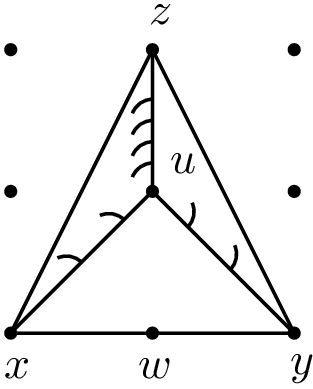
Figure 8. Long description
The diagram depicts a resolved surface with exceptional curves shown as small arcs within the triangles. The triangles are labeled with points x, y, z, w, and u. The arcs within the triangles represent the components of the exceptional curves. The structure includes a central triangle with vertices labeled x, y, and z, and an inner point labeled u connected to the vertices. Additional points and lines extend from the central triangle, indicating the relationships and connections between the components.
Our construction of $\mathcal{LS}$
gives a way to compare
$\mathcal{LS}$
gives a way to compare $\mathcal{LS}_Y$
with
$\mathcal{LS}_Y$
with $\mathcal{LS}_X$
. Denote by
$\mathcal{LS}_X$
. Denote by $S=\operatorname {Sing} X$
and
$S=\operatorname {Sing} X$
and $T=\operatorname {Sing} Y$
the singular sets with the reduced scheme structure; and note that
$T=\operatorname {Sing} Y$
the singular sets with the reduced scheme structure; and note that $f_{|T}\colon T\to S$
is an isomorphism. We use
$f_{|T}\colon T\to S$
is an isomorphism. We use $f_{|T}$
to view
$f_{|T}$
to view $Z$
as a subset of
$Z$
as a subset of $T$
. The resolution was constructed precisely so that the intersection of the union of all exceptional curves with
$T$
. The resolution was constructed precisely so that the intersection of the union of all exceptional curves with $T$
equals
$T$
equals $Z$
. Moreover, we precisely understand how the slab bundles change under this blow-up. A concise way to write this is as follows. The sheaf
$Z$
. Moreover, we precisely understand how the slab bundles change under this blow-up. A concise way to write this is as follows. The sheaf $\mathcal{LS}_Y$
is supported on
$\mathcal{LS}_Y$
is supported on $T$
and
$T$
and $\mathcal{LS}_X$
on
$\mathcal{LS}_X$
on $S$
and we have
$S$
and we have
 \begin{align} \mathcal{LS}_Y = f^{\star} \mathcal{LS}_X (-Z). \end{align}
The slab sections $f_{\rho _x}$
,
$f_{\rho _x}$
, $f_{\rho _y}$
and
$f_{\rho _y}$
and $f_{\rho _z}$
give a section
$f_{\rho _z}$
give a section $s$
of
$s$
of $\mathcal{LS}_X$
in the affine neighbourhood
$\mathcal{LS}_X$
in the affine neighbourhood $u=1$
of the unique joint and this section extends uniquely to all of
$u=1$
of the unique joint and this section extends uniquely to all of $X$
without receiving extra zeros outside the affine chart. The vanishing set of
$X$
without receiving extra zeros outside the affine chart. The vanishing set of $s$
is
$s$
is $Z$
. Therefore, the section
$Z$
. Therefore, the section $s$
is the image of a section
$s$
is the image of a section $\widetilde {s}$
under the natural inclusion
$\widetilde {s}$
under the natural inclusion $\mathcal{LS}_X(-Z)\subset \mathcal{LS}_X$
and, moreover,
$\mathcal{LS}_X(-Z)\subset \mathcal{LS}_X$
and, moreover, $\widetilde {s}$
is nowhere-vanishing. Hence,
$\widetilde {s}$
is nowhere-vanishing. Hence, $\widetilde {s}$
gives a compatible log structure on
$\widetilde {s}$
gives a compatible log structure on $Y$
that is smooth over
$Y$
that is smooth over $k^\dagger$
, in notation
$k^\dagger$
, in notation $Y^\dagger /k^\dagger$
. Furthermore, since
$Y^\dagger /k^\dagger$
. Furthermore, since $\widetilde {s}$
and
$\widetilde {s}$
and $s$
agree over the set
$s$
agree over the set
 \begin{align*} Y\setminus f^{-1} (Z)\overset {f}{=} X\setminus Z. \end{align*}
and $\widetilde {s}$
maps to
$\widetilde {s}$
maps to $s$
under the inclusion
$s$
under the inclusion $\mathcal{LS}_X(-Z)\subset \mathcal{LS}_X$
, we also obtain that the log structure given by
$\mathcal{LS}_X(-Z)\subset \mathcal{LS}_X$
, we also obtain that the log structure given by $\widetilde {s}$
on
$\widetilde {s}$
on $Y\setminus X$
is that given by
$Y\setminus X$
is that given by $s$
on
$s$
on $X\setminus Z$
. The morphism of schemes
$X\setminus Z$
. The morphism of schemes $f\colon Y \to X$
is log crepant in the sense that
$f\colon Y \to X$
is log crepant in the sense that
 \begin{align*} \Omega^2_{Y^\dagger /k^\dagger } \end{align*}
is $f$
-trivial. We say that
$f$
-trivial. We say that $Y^\dagger /k^\dagger$
together with
$Y^\dagger /k^\dagger$
together with $f\colon Y \to X$
is a log crepant log resolution of
$f\colon Y \to X$
is a log crepant log resolution of $X^\dagger$
over
$X^\dagger$
over $k^\dagger$
.
$k^\dagger$
.
5.4 The
$3$
-fold transverse
$A_1$
-singularity


5.4.1 Description of the space and its log structure.
We take $X$
to be the affine cone over the projective toroidal crossing surface of Section 5.3.1: the toroidal crossing
$X$
to be the affine cone over the projective toroidal crossing surface of Section 5.3.1: the toroidal crossing $3$
-fold union of three toric affine pieces given in
$3$
-fold union of three toric affine pieces given in $\mathbb{A}^5$
by the equations
$\mathbb{A}^5$
by the equations
 \begin{align*} X= \left \{ \begin{aligned} xy-w^2 & =0 \\ zw & = 0 \end{aligned} \right. \end{align*}
in affine coordinates $x,y,z,u,w$
. Note that
$x,y,z,u,w$
. Note that $u$
does not appear in the equations:
$u$
does not appear in the equations: $X$
is the product of a toroidal crossing surface with
$X$
is the product of a toroidal crossing surface with $\mathbb{A}^1_u$
.
$\mathbb{A}^1_u$
.
The three components of $X$
are
$X$
are
 \begin{align*} X_1=\left (z=xy-w^2=0\right )\!, \quad X_2=\left (w=x=0\right ) \quad \text{and}\quad X_3=\left (w=y=0\right )\!. \end{align*}
The obvious and, essentially, unique polarization has kink $k=1$
along the coordinate surfaces
$k=1$
along the coordinate surfaces $\mathbb{A}^2_{x,u}$
and
$\mathbb{A}^2_{x,u}$
and $\mathbb{A}^2_{y,u}$
, and
$\mathbb{A}^2_{y,u}$
, and $k=2$
along
$k=2$
along $\mathbb{A}^2_{z,u}$
.
$\mathbb{A}^2_{z,u}$
.
We choose the very special log structure on $X$
over
$X$
over $k^\dagger$
given by the slab sections:
$k^\dagger$
given by the slab sections:
 \begin{align} \begin{aligned} f_{\rho _x} & = u ,\\ f_{\rho _y} & = u ,\\ f_{\rho _z} & = u^2 - z^2. \end{aligned} \end{align}
The joint condition along the $u$
-axis is satisfied. We denote by
$u$
-axis is satisfied. We denote by $X^\dagger /k^\dagger$
the
$X^\dagger /k^\dagger$
the $3$
-fold
$3$
-fold $X$
equipped with the log structure and structure morphism
$X$
equipped with the log structure and structure morphism $X^\dagger \to \operatorname {Spec} k^\dagger$
given by these slab sections.
$X^\dagger \to \operatorname {Spec} k^\dagger$
given by these slab sections.
The singular locus of $X$
has three irreducible components as follows:
$X$
has three irreducible components as follows:
 \begin{align*} S_1= & \mathbb{A}^2_{z,u}=X_2\cap X_3,\\ S_2= & \mathbb{A}^2_{x,u}=X_1\cap X_3,\\ S_3= & \mathbb{A}^2_{y,u}=X_1\cap X_2. \end{align*}
The structure morphism $\pi \colon X^\dagger \to \operatorname {Spec} k^\dagger$
is singular along the locus
$\pi \colon X^\dagger \to \operatorname {Spec} k^\dagger$
is singular along the locus $Z\subset X$
where the slab sections vanish. This singular locus (see Figure 9) has three irreducible components as follows:
$Z\subset X$
where the slab sections vanish. This singular locus (see Figure 9) has three irreducible components as follows:
 \begin{align*} Z_1 =(u^2-z^2=0)\subset S_1, \quad \end{align*}
 \begin{align*} Z_2 =(u=0) \subset S_2, \quad \end{align*}
 \begin{align*} Z_3 =(u=0) \subset S_3. \end{align*}
5.4.2 Log deformations of
$X^\dagger /k^\dagger$
.

Consider the family of $3$
-folds over
$3$
-folds over $\mathbb{A}^1$
with coordinate
$\mathbb{A}^1$
with coordinate $t$
given by the equations
$t$
given by the equations
 \begin{align} \mathfrak{X} = \left \{ \begin{aligned} xy-w^2 & =-t^2\\ zw & = tu \end{aligned} \right. \end{align}
in $\mathbb{A}^5\times \mathbb{A}^1$
, together with the projection
$\mathbb{A}^5\times \mathbb{A}^1$
, together with the projection $\pi \colon \mathfrak{X} \to \mathbb{A}^1$
. The equations describe a smoothing of
$\pi \colon \mathfrak{X} \to \mathbb{A}^1$
. The equations describe a smoothing of $X$
; and the restriction to
$X$
; and the restriction to $X$
of the divisorial log structure
$X$
of the divisorial log structure $\mathfrak{M}_{\mathfrak{X}, X}$
is that given in (5.6).
$\mathfrak{M}_{\mathfrak{X}, X}$
is that given in (5.6).
5.4.3 Log crepant log resolutions.
The following facts are elementary and easy to verify. We construct a $3$
-fold
$3$
-fold $Y$
and proper birational morphism
$Y$
and proper birational morphism $f\colon Y \to X$
as follows. First let
$f\colon Y \to X$
as follows. First let $Y_2\to X_2$
be the blow up of the singular curve
$Y_2\to X_2$
be the blow up of the singular curve $Z_3\subset X_2$
.
$Z_3\subset X_2$
.
Next let $Y_3\to X_3$
be as follows:
$Y_3\to X_3$
be as follows:
-
– first, let
$f^\prime \colon Y_3^\prime \to X_3$
be the blow up of the curve
$Z_2\subset X_3$
, and -
– second, let
$Y_3 \to Y_3^\prime$
be the blow up of the strict transform
$Z_1^\prime \subset Y_3^\prime$
of the curve
$Z_1\subset X_3$
given by
$(u^2-z^2=0)\subset \mathbb{A}^2_{z, u}$
; note that
$Z_1^\prime$
is nonsingular and consists of two components that we call
$Z_+$
,
$Z_-$
corresponding to the factors
$u+z$
,
$u-z$
.





Denote by $Y$
be the
$Y$
be the $3$
-fold obtained by re-assembling the three components
$3$
-fold obtained by re-assembling the three components $Y_1=X_1$
,
$Y_1=X_1$
, $Y_2$
,
$Y_2$
, $Y_3$
in the obvious way (see Figure 10); and by
$Y_3$
in the obvious way (see Figure 10); and by $f\colon Y \to X$
the obvious proper birational morphism.
$f\colon Y \to X$
the obvious proper birational morphism.
The log singular locus of $X^\dagger$
.
$X^\dagger$
.
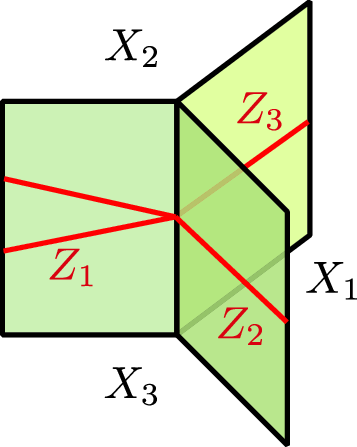
Figure 9. Long description
The diagram features three intersecting geometric shapes. The shapes are labeled X1, X2, and X3. Within these shapes, there are additional regions labeled Z1, Z2, and Z3. Red lines connect these regions, indicating relationships or transitions between them. The shapes and lines form a complex structure, suggesting a mathematical or scientific concept related to smoothing singular log schemes.
Schematic of the resolution.

Figure 10. Long description
The schematic diagram illustrates the resolution process, featuring multiple labeled components and their interactions. The diagram includes green planes labeled Y2 and Y3, intersecting with other planes labeled X1, Z2, and Z3. There are two intersecting purple planes labeled Z+ and Z-. Red and orange shaded regions represent areas of intersection and overlap between these planes. The diagram visually represents the relationships and connections between these components, providing a structured overview of the resolution framework.
Our construction of $\mathcal{LS}$
gives a way to compare
$\mathcal{LS}$
gives a way to compare $\mathcal{LS}_Y$
with
$\mathcal{LS}_Y$
with $f^{\star} (\mathcal{LS}_X)$
, which we next explain. Denote by
$f^{\star} (\mathcal{LS}_X)$
, which we next explain. Denote by $T=\operatorname {Sing} Y$
the singular set with the reduced scheme structure;
$T=\operatorname {Sing} Y$
the singular set with the reduced scheme structure; $T$
consists of three irreducible components
$T$
consists of three irreducible components
 \begin{align*} T_1=Y_2\cap Y_3, \quad T_2=Y_3\cap Y_1,\quad T_3= Y_1\cap Y_3. \end{align*}
We have that $f_{|T_1} \colon T_1\to S_1$
is the blow up of the origin,
$f_{|T_1} \colon T_1\to S_1$
is the blow up of the origin, $f_{|T_2}\colon T_2\to S_2$
is an isomorphism, and so is
$f_{|T_2}\colon T_2\to S_2$
is an isomorphism, and so is $f_{|T_3}\colon T_3\to S_3$
.
$f_{|T_3}\colon T_3\to S_3$
.
Next we identify the slab line bundles $\mathcal{L}_{Y,1}$
,
$\mathcal{L}_{Y,1}$
, $\mathcal{L}_{Y,2}$
,
$\mathcal{L}_{Y,2}$
, $\mathcal{L}_{Y,3}$
on
$\mathcal{L}_{Y,3}$
on $T_1$
,
$T_1$
, $T_2$
,
$T_2$
, $T_3$
.
$T_3$
.
We need a notation for the exceptional divisors of the morphisms $Y_i\to X_i$
. The first of these morphisms,
$Y_i\to X_i$
. The first of these morphisms, $f_{|Y_1}\colon Y_1\to X_1$
, is an isomorphism, so there is nothing to be done here. Denote by
$f_{|Y_1}\colon Y_1\to X_1$
, is an isomorphism, so there is nothing to be done here. Denote by $E_2\subset Y_2$
the exceptional divisor of
$E_2\subset Y_2$
the exceptional divisor of $f_{|Y_2}\colon Y_2\to X_2$
, so
$f_{|Y_2}\colon Y_2\to X_2$
, so $E_2$
is a
$E_2$
is a $\mathbb{P}^1$
-bundle over
$\mathbb{P}^1$
-bundle over $Z_3$
. The exceptional divisor of
$Z_3$
. The exceptional divisor of $f_{|Y_3}\colon Y_3\to X_3$
consists of three components: the strict transform
$f_{|Y_3}\colon Y_3\to X_3$
consists of three components: the strict transform $E_3$
of the exceptional divisor of
$E_3$
of the exceptional divisor of $f^\prime \colon Y_3^\prime \to X_3$
, and the divisors
$f^\prime \colon Y_3^\prime \to X_3$
, and the divisors $F_+$
,
$F_+$
, $F_-$
that dominate the curves
$F_-$
that dominate the curves $u+z=0$
,
$u+z=0$
, $u-z=0$
in
$u-z=0$
in $S_1$
.
$S_1$
.
We denote by $\Xi = E_{2}\cap T_1 = E_{3}\cap T_1\subset T_1$
the exceptional divisor of
$\Xi = E_{2}\cap T_1 = E_{3}\cap T_1\subset T_1$
the exceptional divisor of $T_1\to S_1$
, and we write
$T_1\to S_1$
, and we write $Z_+=F_{+}\cap T_1$
,
$Z_+=F_{+}\cap T_1$
, $Z_-=F_{-}\cap T_1$
. Note that
$Z_-=F_{-}\cap T_1$
. Note that
 \begin{align*} (f_{|T_1})^\star (Z_1) = F_++F_- + 2\Xi.\end{align*}
With this notation in hand we are ready to compute the slab bundles. The Stanley–Reisner ring along the joint $u$
is given by the fan at the monomial
$u$
is given by the fan at the monomial $u$
in Figure 7. We see that the monomials
$u$
in Figure 7. We see that the monomials $xz$
and
$xz$
and $yz$
correspond to opposite lattice vectors, so we can use them to compute the slab bundle on
$yz$
correspond to opposite lattice vectors, so we can use them to compute the slab bundle on $T_1$
. We also see from the figure that the monomial
$T_1$
. We also see from the figure that the monomial $xz$
defines the boundary divisor
$xz$
defines the boundary divisor $\partial Y_3$
on
$\partial Y_3$
on $Y_3$
and the monomial
$Y_3$
and the monomial $yz$
defines the boundary divisor
$yz$
defines the boundary divisor $\partial Y_2$
on
$\partial Y_2$
on $Y_2$
, so we arrive at
$Y_2$
, so we arrive at
 \begin{align*} \mathcal{L}_{Y,1} & =\mathcal{O}_{Y_2}(\partial Y_2)_{|T_1}\otimes \mathcal{O}_{Y_3}(\partial Y_3)_{|T_1}=(N_{Y_2} T_1) \otimes (N_{Y_3} T_1) \otimes \mathcal{O}_{T_1} (2Y_1) \\ & =(f^{\star} N_{X_2} S_1) \otimes (f^{\star} N_{X_3} S_1) (-F_+-F_-) \otimes \mathcal{O}_{S_1} (2X_1)(-2\Xi ) \\ & =(f^{\star} \mathcal{L}_{X_1})(-F_+-F_- -2\Xi ) = f^{\star} \bigl (\mathcal{L}_{X,1}(-Z_1)\bigr ). \end{align*}
The formulas for $\mathcal{L}_{Y,2}$
and
$\mathcal{L}_{Y,2}$
and $\mathcal{L}_{Y,3}$
are much easier to understand:
$\mathcal{L}_{Y,3}$
are much easier to understand:
 \begin{align*} \mathcal{L}_{Y,2}=\mathcal{L}_{X,2}(-Z_2), \quad \mathcal{L}_{Y,3} = \mathcal{L}_{X,3} (-Z_3). \end{align*}
We summarize these calculations with the formula
 \begin{align} \mathcal{LS}_Y=f^{\star} \bigl ( \mathcal{LS}_X(-Z)\bigr ). \end{align}
Pulling back the section of $\mathcal{LS}_X$
defined by the slab sections (5.6) results in a nowhere-vanishing section of
$\mathcal{LS}_X$
defined by the slab sections (5.6) results in a nowhere-vanishing section of $\mathcal{LS}_Y$
. We see from this the following.
$\mathcal{LS}_Y$
. We see from this the following.
-
(1) There is a unique log structure on
$Y$
over
$k^\dagger$
that onis the given one on
\begin{align*} Y\setminus f^{-1}(Z) \overset {f}{=} X\setminus Z \end{align*}
$X\setminus Z$
;
-
(2) The resulting log scheme
$Y^\dagger /k^\dagger$
is log smooth over
$\operatorname {Spec} k^\dagger$
.


One can check that the resulting morphism $Y \to X$
is log crepant, so it gives a log crepant log resolution of
$Y \to X$
is log crepant, so it gives a log crepant log resolution of $X^\dagger$
over
$X^\dagger$
over $k^\dagger$
.
$k^\dagger$
.
This example shows how the sheaf $\mathcal{LS}_X$
can be used in constructing log smooth resolutions.
$\mathcal{LS}_X$
can be used in constructing log smooth resolutions.
Acknowledgements
We are grateful to Simon Felten and Andrea Petracci for many useful discussions on the subject of this paper. We thank Kevin Buzzard, Simon Felten, Martin Olsson, Bernd Siebert, Mattia Talpo, Anna-Maria Raukh and an anonymous referee for comments on earlier versions of this article and helpful suggestions at various stages of the long revision process.
Kevin had a strong influence on shaping our view of the subject; in particular, he explained to us that the words ‘canonical’, ‘natural’, distinguished’, etc. are meaningless, see [Reference BuzzardBuz25]. As a result of our conversations with him, we eliminated all occurrences of these words in the text, and instead we made the effort of stating all the properties that our constructions need to satisfy. Kevin also explained to us some key points about coherence theorems in monoidal categories.
The authors were hosted by Mathematisches Forschungsinstitut Oberwolfach as Oberwolfach Research Fellows in 2021 and 2022. Substantial parts of the work on this project were produced during these retreats. Gratitude for hospitality also goes to the Department of Mathematics at Imperial College London, the University of Hamburg and the Department of Mathematics and Physics at the University of Stavanger.
Financial support
A.C. received support from an EPSRC Programme Grant EP/N03189X/1. H.R. received support from the grants DFG RU 1629/4-1 and NFR Fripro Shape2030.
Conflicts of interest
None.
Journal information
Moduli is published as a joint venture of the Foundation Compositio Mathematica and the London Mathematical Society. As not-for-profit organisations, the Foundation and Society reinvest $100\%$
of any surplus generated from their publications back into mathematics through their charitable activities.
$100\%$
of any surplus generated from their publications back into mathematics through their charitable activities.









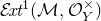




















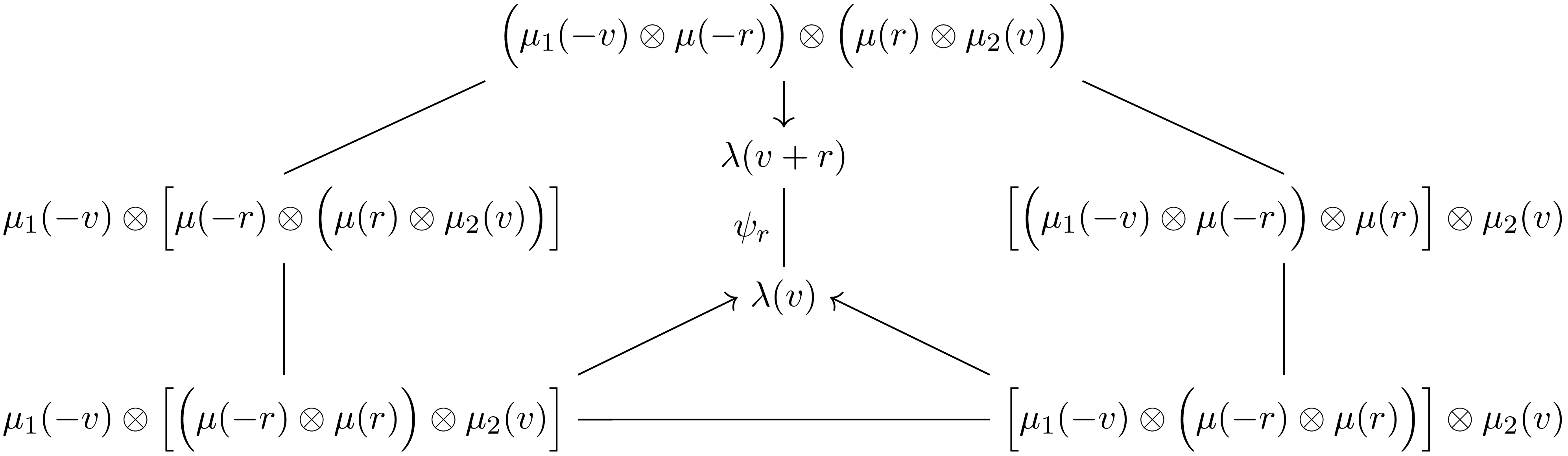
 ψr:λ(v)→λ(r+v)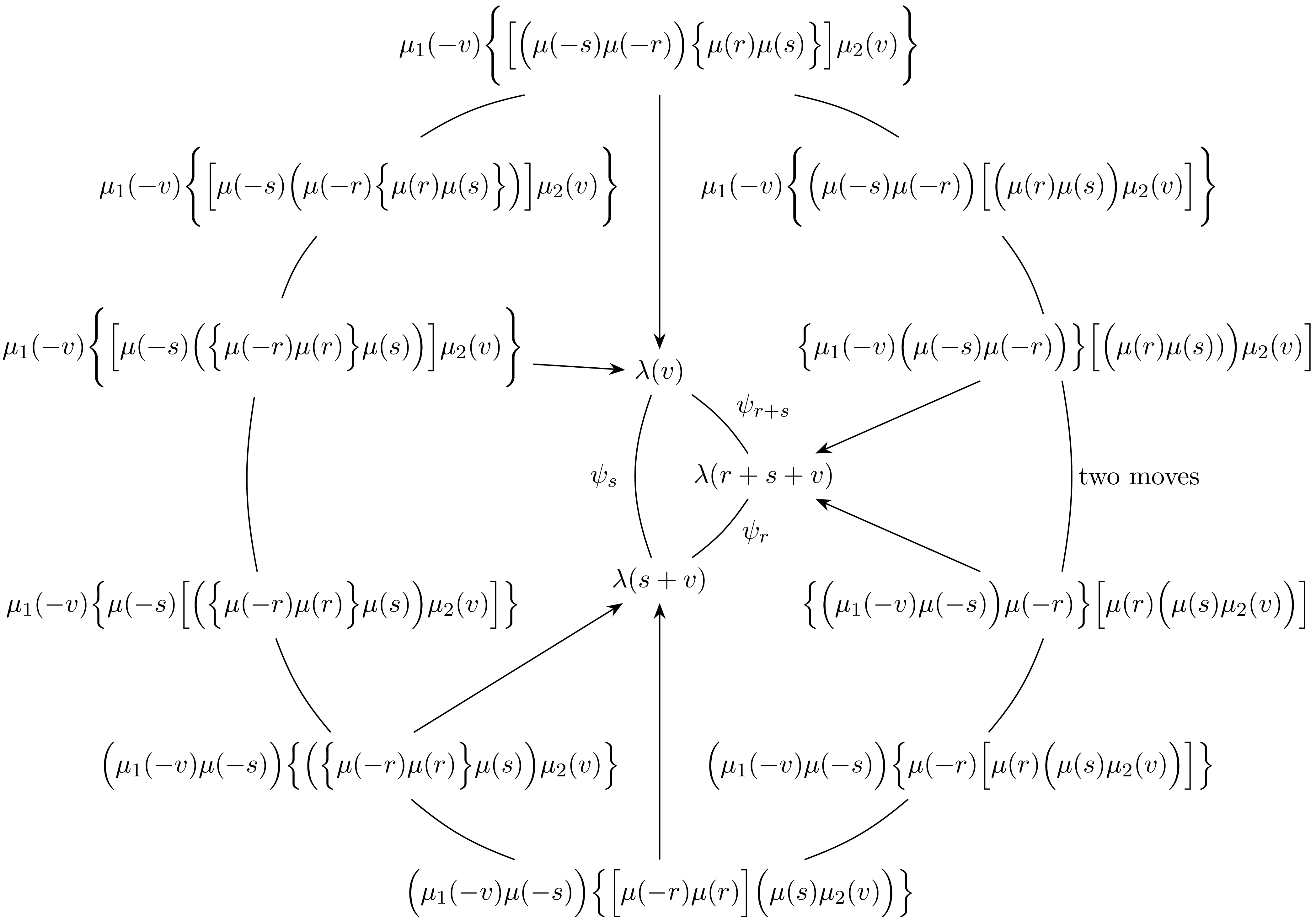
 ψr+s=ψr∘ψs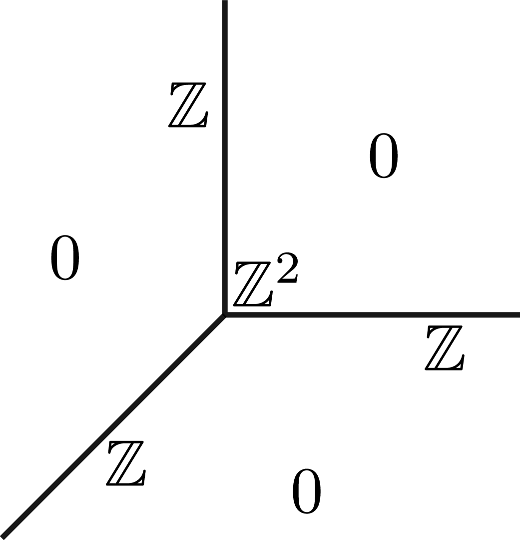
 M=Pgp/1
 T
T xyz=0
xyz=0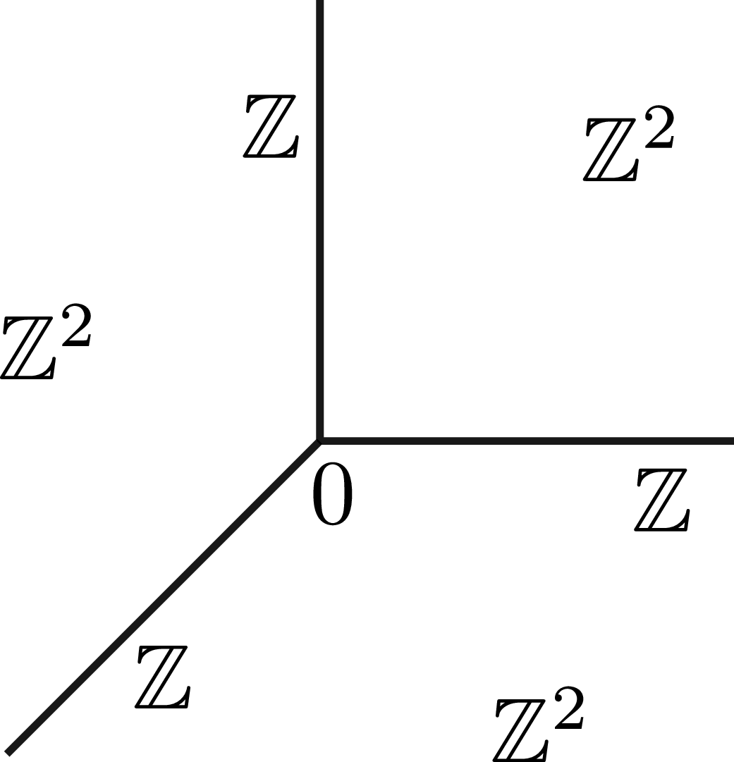
 R
R T
T xyz=0
xyz=0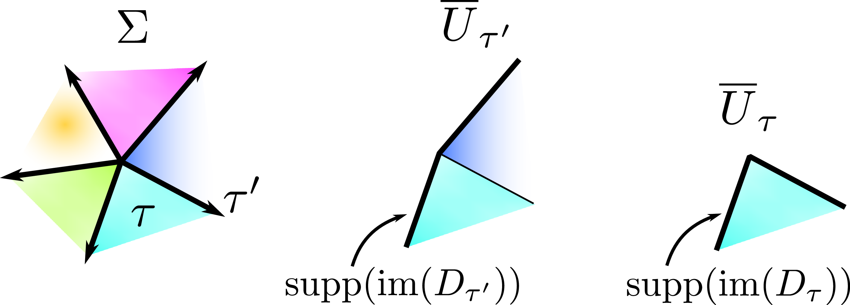
 U¯τ⊂U¯τ′
 τ′⩽τ
τ′⩽τ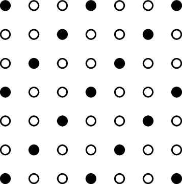
 M⊂Z2
M⊂Z2 r=3
r=3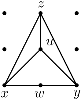
 X
X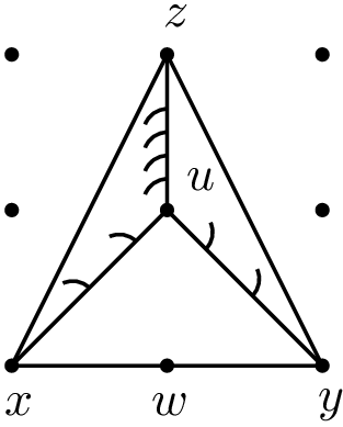
 Y
Y Y
Y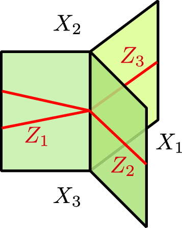
 X†
X†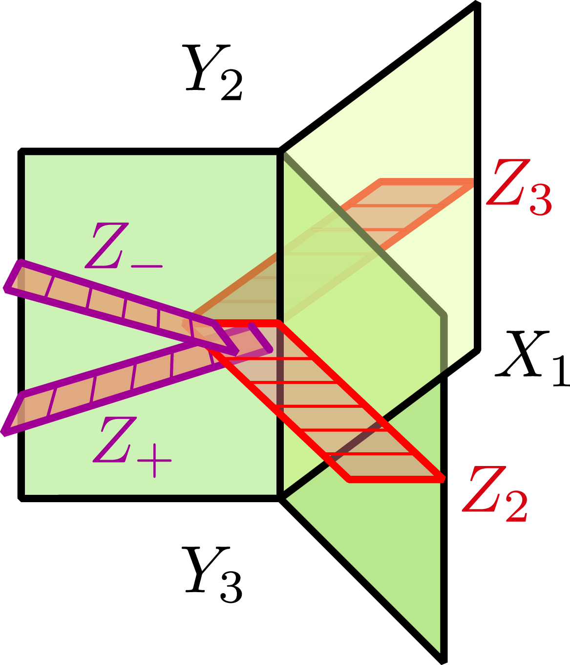

 Open access

