


I. Introduction
The neoclassical theory of investment has a long history. It has been developed, tested, and refined across many decades since the seminal work of Jorgenson (Reference Jorgenson1963) and Tobin (Reference Tobin1969). The neoclassical theory suggests that the rate of investment is a function of Tobin’s q, measured by the ratio of the market value of new additional investment goods to their replacement cost, an intuition that goes back to Keynes (Reference Keynes1936). The foundation of modern q theory in Lucas and Prescott (Reference Lucas and Prescott1971) and Mussa (Reference Mussa1977) is the firm’s optimization condition—the marginal adjustment and direct purchasing costs of investment being equal to the shadow value of capital. Relatedly, Hayashi (Reference Hayashi1982) shows that marginal q equals average q under standard assumptions. Average q is the usual empirical measure of q, defined as the ratio of the valuation of the firm’s existing capital stock to its replacement cost, and it is prone to measurement issues. However, some recent studies challenge the empirical applicability of the q theory, citing difficulties in accurately measuring q, and propose alternative approaches that predict firms’ investment decisions.
In this article, we investigate the relationship between a firm’s investment and q, for which an unobserved persistent shock to the investment cost function, such as information or technology shock, is an important factor in the firm’s investment decision, derived from the firm’s optimization problem. In our dynamic investment model to motivate the empirical investment equation, both the capital and the unobserved persistent shock are dynamic state variables; risk-neutral firms choose investment each period seeking to maximize the expected present value of their continuing future profits. For example, in this setting, firms experiencing a positive technology shock may face lower investment adjustment costs. Technological advances make equipment less expensive, make the investment process more efficient, and lead to improvements in the real investment opportunity set (Greenwood, Hercowitz, and Krusell (Reference Greenwood, Hercowitz and Krusell1997), Stiroh (Reference Stiroh2002), Fisher (Reference Fisher2006), and Kogan and Papanikolaou (Reference Kogan and Papanikolaou2014)). As a result, the q-measure may become endogenous in the firm’s investment equation if the unobserved shock is not properly accounted for. Importantly, we argue that incorporating the unobserved shock into the optimal investment function is essential, as this shock may directly impact capital adjustment costs, rather than solely influencing the firm’s production function. Nonetheless, we demonstrate that this channel of dependency is not precluded by the existing classical investment theory.
The empirical concern we address here is a new challenge to the potential measurement problem of marginal q. It has been studied relatively well in the literature (e.g., Hayashi (Reference Hayashi1982), Blanchard, Rhee, and Summers (Reference Blanchard, Rhee and Summers1993), and Erickson and Whited (Reference Erickson and Whited2000)), compared to the potential omitted variable problem we focus on. Unfortunately, controlling for measurement error in marginal q alone has been proven to be a difficult problem in the literature, as different empirical approaches taken to measurement errors rendered various and even contradictory conclusions on the roles of marginal q and internal funds in investment decisions. Addressing both the unobserved persistent shock and the measurement error problem is even more challenging. If the shock is omitted, not only does q become endogenous, but other observed regressors, such as cash flow or leverage, may also become endogenous. This underscores the critical importance of controlling for the unobserved persistent shock to estimate the investment function consistently.
To this end, we develop an econometric method that handles both issues. Our approach allows for time-varying investment adjustment costs and direct investment costs in firm-level panel data. Our identification strategy is based on a set of timing and information set assumptions about changes in the unobserved shock and adjustment costs. Given these restrictions, we derive moment conditions under which we identify both investment function parameters and dynamic parameters of the unobserved shock, and propose a Generalized Method of Moments (GMM) estimator. Our approach is robust to the endogeneity concerns in estimating the investment functions, where q is correlated with the unobserved persistent shock and subject to measurement error.
Methodologically, we utilize a panel data approach, building on a similar method proposed by Blundell and Bond (Reference Blundell and Bond1998), (Reference Blundell and Bond2000) and Bajari, Fruehwirth, Kim, and Timmins (Reference Bajari, Fruehwirth, Kim and Timmins2012). Our estimation approach also generalizes differencing approaches used to control for correlated time-varying confounders. However, our context and problems are substantially different from those of existing studies. This is because, in the context of investment functions, not only is q mismeasured, but also the unobserved persistent shock is potentially correlated with other factors of investment, such as q. In standard dynamic panel models, endogeneity arises because differencing to remove a firm fixed effect induces correlation between the lagged dependent variable as a regressor and the differenced error term. In our investment equation, this endogeneity is present regardless of a firm fixed effect.
To motivate our insights on the unobserved persistent shock, we begin by incorporating the firm’s estimated total factor productivity (TFP) as an additional regressor and estimate the augmented investment equation. For this purpose, we utilize the TFP measure from İmrohoroǧlu and Tüzel (Reference İmrohoroǧlu and Tüzel2014), who estimate firm-level production functions using Olley and Pakes (Reference Olley and Pakes1996).Footnote 1 In particular, we estimate the investment equation both with and without TFP included as an additional observed state variable to assess whether our approach can effectively account for TFP when it is unobserved. We first proceed with a GMM estimator by including TFP as an additional observed state variable in place of the unobserved persistent shock. The results show that both q and TFP are statistically significant. We next estimate the investment equation using our proposed method to account for the unobserved persistent shock. It suggests that the unobserved persistent shock is significant. Importantly, q continues to be a significant factor even after the unobserved persistent shock is being controlled for. Lastly, to examine whether TFP contains information beyond that captured by the unobserved persistent shock, we include both TFP and the persistent shock in the investment function. Interestingly, once the unobserved shock is accounted for, TFP is no longer statistically significant. This suggests that our proposed method effectively captures the influence of the unobserved persistent shock, such as cost or technology shock, on investment decisions.Footnote 2


We also examine the investment equation both with and without controlling for measurement error in q. When the measurement error is ignored, the estimated coefficient on q is substantially smaller than when the error is properly accounted for. This highlights the importance and empirical relevance of addressing both the omitted persistent shock and measurement error. We also consider a case where the measurement error follows a more persistent process than the one assumed in our benchmark model. The estimation results remain very similar under this generalization, suggesting that our baseline specification performs effectively in the empirical setting.
We then conduct extensive empirical analyses, utilizing various measures of investment and q (for both physical and intangible measures) used in recent literature, for example, Peters and Taylor (Reference Peters and Taylor2017). Using 16,256 unique firms from 1975 to 2021, our empirical results indicate the importance of controlling for the unobserved persistent shock in estimating investment functions. Across all investment equations considered, we find that the unobserved persistent shock plays a significant role. Importantly, our finding indicates that q is still a significant factor in investment decisions, even after controlling for the unobserved persistent shock and measurement error in q.
We contribute to the literature on the empirics of corporate investment in several significant dimensions. First, to motivate our specification of the investment equation, we allow a firm’s adjustment cost of capital stock to depend on its unobserved persistent shock. We demonstrate that the optimal investment model is not only determined by q and other state variables but also by the unobserved persistent shock.
Second, we develop an estimation strategy for investment functions accounting for both endogeneity concerns due to the unobserved persistent shock and possibly mismeasured q. Our identifying moment conditions are derived from timing and information set assumptions that align with the firm’s optimal decision-making process and are well grounded in the principle of rational expectations. Moreover, our estimator is straightforward to implement using standard computing software. We offer a set of diagnostic tests for the moment conditions.
Third, our empirical analysis confirms that q remains an important factor of investment even when other state variables such as firm size, employment, and cash flow (or leverage) are controlled for. Furthermore, we find that investment becomes more sensitive to q after accounting for the unobserved persistent shock and the measurement error problems. This result holds for our subperiod analysis, alternative definitions of investment and q, and a variety of robustness checks.
The rest of the article proceeds as follows: Section II presents an investment model extending the models in Lucas and Prescott (Reference Lucas and Prescott1971) and Mussa (Reference Mussa1977), in which the unobserved persistent shock factors into a firm’s investment. Section III develops estimation methods. Section IV describes the data and variable construction. Section V reports the estimation results, and Section VI concludes.
II. Investment Model
To develop an empirical framework for an endogenous q model of investment in which both capital and the unobserved persistent shock are dynamic state variables, we present a simple standard dynamic investment model where risk-neutral firms choose investments each period to maximize the expected present value of continuing future profits. We use this simple dynamic investment model to motivate estimable equations and to discuss the nature of endogeneity problems in our empirical framework.
A. q Theory of Optimal Investment with Unobserved Shocks
We build on the original setting of Lucas and Prescott (Reference Lucas and Prescott1971) and Mussa (Reference Mussa1977) but, as an important point of departure, we allow for the unobserved persistent shock to enter the investment cost function. Here, we modify the dynamic investment model in Erickson and Whited (Reference Erickson and Whited2000), in which capital is the endogenous quasi-fixed factor and the unobserved persistent shock is another fixed factor that evolves exogenously following a dynamic process (e.g., a first-order Markov process). The value of the firm $ i $
at time
$ i $
at time $ t $
, from which the firm derives its optimal decision on investment to maximize the expected present value of the discounted flow of future profits, is given by
$ t $
, from which the firm derives its optimal decision on investment to maximize the expected present value of the discounted flow of future profits, is given by
 $$ {V}_{it}=E\left[\sum \limits_{j=0}^{\infty}\left(\prod \limits_{s=1}^j{b}_{i,t+s}\right)\left[{\Pi}_{t+j}\left({K}_{i,t+j},{\varsigma}_{i,t+j}\right)-\psi \right({I}_{i,t+j},{K}_{i,t+j},{W}_{i,t+j},{\nu}_{i,t+j}\Big)|{\Omega}_{it}\right]. $$
Here, $ E\left[\cdot |{\Omega}_{it}\right] $
is the conditional expectation operator and
$ E\left[\cdot |{\Omega}_{it}\right] $
is the conditional expectation operator and $ {\Omega}_{it} $
denotes the information set available to firm i at time t;
$ {\Omega}_{it} $
denotes the information set available to firm i at time t; $ {K}_{it} $
is the capital stock available at the beginning of period
$ {K}_{it} $
is the capital stock available at the beginning of period $ t $
;
$ t $
; $ {I}_{it} $
is the investment and
$ {I}_{it} $
is the investment and $ {b}_{it} $
is the firm’s discount factor at time
$ {b}_{it} $
is the firm’s discount factor at time $ t $
;
$ t $
; $ {\Pi}_t\left({K}_{it},{\varsigma}_{it}\right) $
is the per period profit function, increasing in
$ {\Pi}_t\left({K}_{it},{\varsigma}_{it}\right) $
is the per period profit function, increasing in $ {K}_{it} $
, with
$ {K}_{it} $
, with $ {\varsigma}_{it} $
being the shock to the profit function;
$ {\varsigma}_{it} $
being the shock to the profit function; $ \psi \left({I}_{it},{K}_{it},{W}_{it},{\nu}_{it}\right) $
is the investment cost function including both the cost of adjusting the stock of capital and the direct purchase or sale cost of investment, where
$ \psi \left({I}_{it},{K}_{it},{W}_{it},{\nu}_{it}\right) $
is the investment cost function including both the cost of adjusting the stock of capital and the direct purchase or sale cost of investment, where $ {\nu}_{it} $
is an exogenous shock to adjustment cost.
$ {\nu}_{it} $
is an exogenous shock to adjustment cost. $ {W}_{it} $
denotes the vector of state variables other than capitals, which may include technology shock, demand and cost shocks, and other aggregate shocks.
$ {W}_{it} $
denotes the vector of state variables other than capitals, which may include technology shock, demand and cost shocks, and other aggregate shocks.
The cost function $ \psi \left({I}_{it},{K}_{it},{W}_{it},{\nu}_{it}\right) $
is increasing in
$ \psi \left({I}_{it},{K}_{it},{W}_{it},{\nu}_{it}\right) $
is increasing in $ {I}_{it} $
, decreasing in
$ {I}_{it} $
, decreasing in $ {K}_{it} $
, and convex in the first two arguments. The shocks
$ {K}_{it} $
, and convex in the first two arguments. The shocks $ \left({\varsigma}_{it},{\nu}_{it}\right) $
and state variables
$ \left({\varsigma}_{it},{\nu}_{it}\right) $
and state variables $ {W}_{i,t} $
are observed by the firm at time
$ {W}_{i,t} $
are observed by the firm at time $ t $
, but these shocks and some components of
$ t $
, but these shocks and some components of $ {W}_{it} $
may not be fully observed by the econometrician. Finally, note that any other variable factors of production in the profit function (e.g., labor or materials) have already been optimized following static optimization problems by the firm. Also, for ease of notation, other observed factors are implicit and suppressed. For estimation, we will decompose
$ {W}_{it} $
may not be fully observed by the econometrician. Finally, note that any other variable factors of production in the profit function (e.g., labor or materials) have already been optimized following static optimization problems by the firm. Also, for ease of notation, other observed factors are implicit and suppressed. For estimation, we will decompose $ {W}_{it} $
into observed factors and the unobserved persistent shock. We will add these additional factors in our empirical investment equation specifications later.
$ {W}_{it} $
into observed factors and the unobserved persistent shock. We will add these additional factors in our empirical investment equation specifications later.
The firm maximizes the expected present value of the future profits $ {V}_{it} $
, subject to the capital stock accumulation identity
$ {V}_{it} $
, subject to the capital stock accumulation identity
 $$ {K}_{i,t+1}=\left(1-{d}_i\right){K}_{it}+{I}_{it}, $$
where $ {d}_i $
is the firm i’s capital depreciation. We then obtain the “marginal”
$ {d}_i $
is the firm i’s capital depreciation. We then obtain the “marginal” $ {q}_{it} $
from
$ {q}_{it} $
from $ \frac{\partial {V}_{it}}{\partial {K}_{it}} $
, which measures the benefit of adding an incremental unit of capital to the firm. The first-order condition for maximizing the value of the firm in equation (1), subject to equation (2), then yields
$ \frac{\partial {V}_{it}}{\partial {K}_{it}} $
, which measures the benefit of adding an incremental unit of capital to the firm. The first-order condition for maximizing the value of the firm in equation (1), subject to equation (2), then yields
 $$ \frac{\partial \psi \left(\cdot \right)}{\partial {I}_{it}}\equiv {\psi}_I\left({I}_{it},{K}_{it},{W}_{it},{\nu}_{it}\right)={q}_{it}. $$
In the original setting of Lucas and Prescott (Reference Lucas and Prescott1971) and Mussa (Reference Mussa1977) (see also Erickson and Whited (Reference Erickson and Whited2000)), which is common in the literature, a firm’s unobserved persistent shock does not enter the investment cost function. Our main innovation is to incorporate an additional source of unobserved firm heterogeneity into the firm’s investment decision problem. We develop an empirical investment equation that aligns with the theoretical model and propose a consistent estimation procedure that accounts for this unobserved factor. Importantly, our framework allows the unobserved persistent shock to influence the optimal investment decision not only through the production function but also by affecting the cost of investment. We argue that this feature remains consistent with the neoclassical theory of investment. The first-order condition above (equation (3)) highlights that incorporating the unobserved shock into the investment cost function $ \psi \left(\cdot \right) $
is essential for the dependence of the optimal investment on the unobserved shock, given the marginal
$ \psi \left(\cdot \right) $
is essential for the dependence of the optimal investment on the unobserved shock, given the marginal $ {q}_{it} $
. This is because the direct impact of this shock on the firm’s profit function
$ {q}_{it} $
. This is because the direct impact of this shock on the firm’s profit function $ {\Pi}_t(\cdot ) $
through its production function is already subsumed in
$ {\Pi}_t(\cdot ) $
through its production function is already subsumed in $ {q}_{it} $
, and the unobserved shock only shows up in the optimal investment through
$ {q}_{it} $
, and the unobserved shock only shows up in the optimal investment through $ \psi \left(\cdot \right) $
as in equation (3).
$ \psi \left(\cdot \right) $
as in equation (3).
B. Empirical Model of Investment Equation
To develop an empirical framework, we now present an investment equation consistent with the firm’s optimal investment decision problem in equation (1). Write $ {W}_{it}\equiv \left({Z}_{it},{\omega}_{it}\right) $
where
$ {W}_{it}\equiv \left({Z}_{it},{\omega}_{it}\right) $
where $ {Z}_{it} $
represents the observed state variables, which may proxy for firm heterogeneity and demand factors, and
$ {Z}_{it} $
represents the observed state variables, which may proxy for firm heterogeneity and demand factors, and $ {\omega}_{it} $
denotes the unobserved persistent shock. We consider a class of investment cost functions, including the cost of adjusting the stock of capital, as
$ {\omega}_{it} $
denotes the unobserved persistent shock. We consider a class of investment cost functions, including the cost of adjusting the stock of capital, as
 $$ \psi \left({I}_{it},{K}_{it},{W}_{it},{\nu}_{it}\right)={K}_{it}\left[{\tilde{f}}_0\left({Z}_{it},{\nu}_{it},{\omega}_{it}\right)+{\tilde{f}}_1\Big({Z}_{it},{\nu}_{it},{\omega}_{it}\Big)\frac{I_{it}}{K_{it}}+\frac{\gamma_{it}}{2}{\left(\frac{I_{it}}{K_{it}}\right)}^2\right], $$
where, in particular, $ {\tilde{f}}_1\left({Z}_{it},{\nu}_{it},{\omega}_{it}\right) $
denotes the linear adjustment cost.
$ {\tilde{f}}_1\left({Z}_{it},{\nu}_{it},{\omega}_{it}\right) $
denotes the linear adjustment cost.
From equation (4), it is clear that the feature of the model that renders the investment function to depend on $ {\omega}_{it} $
is specifically due to the linear adjustment cost
$ {\omega}_{it} $
is specifically due to the linear adjustment cost $ {\tilde{f}}_1\left({Z}_{it},{\nu}_{it},{\omega}_{it}\right) $
, which is a function of the shock
$ {\tilde{f}}_1\left({Z}_{it},{\nu}_{it},{\omega}_{it}\right) $
, which is a function of the shock $ {\omega}_{it} $
, not merely due to the investment cost function
$ {\omega}_{it} $
, not merely due to the investment cost function $ \psi \left({I}_{it},{K}_{it},{W}_{it},{\nu}_{it}\right) $
depending on
$ \psi \left({I}_{it},{K}_{it},{W}_{it},{\nu}_{it}\right) $
depending on $ {\omega}_{it} $
. For example, if we have
$ {\omega}_{it} $
. For example, if we have $ {\tilde{f}}_1\left({Z}_{it},{\nu}_{it},{\omega}_{it}\right)={\tilde{f}}_1\left({Z}_{it},{\nu}_{it}\right) $
, the cost function still depends on
$ {\tilde{f}}_1\left({Z}_{it},{\nu}_{it},{\omega}_{it}\right)={\tilde{f}}_1\left({Z}_{it},{\nu}_{it}\right) $
, the cost function still depends on $ {\omega}_{it} $
because of
$ {\omega}_{it} $
because of $ {\tilde{f}}_0\left({Z}_{it},{\nu}_{it},{\omega}_{it}\right) $
, but this additive adjustment cost does not enter the investment equation as we can see in equation (5). In the literature, it is also typically assumed that the adjustment cost parameter
$ {\tilde{f}}_0\left({Z}_{it},{\nu}_{it},{\omega}_{it}\right) $
, but this additive adjustment cost does not enter the investment equation as we can see in equation (5). In the literature, it is also typically assumed that the adjustment cost parameter $ {\gamma}_{it} $
is constant across firms as
$ {\gamma}_{it} $
is constant across firms as $ \gamma $
(but it may vary by the time
$ \gamma $
(but it may vary by the time $ t $
). Combining these, we obtain
$ t $
). Combining these, we obtain
 $$ \frac{\partial \psi \left(\cdot \right)}{\partial {I}_{it}}\equiv {\psi}_I\left({I}_{it},{K}_{it},{W}_{it},{\nu}_{it}\right)={\tilde{f}}_1\left({Z}_{it},{\nu}_{it},{\omega}_{it}\right)+\gamma \frac{I_{it}}{K_{it}}={q}_{it}. $$
This equation clearly indicates that $ {q}_{it} $
is dependent on the unobserved persistent shock
$ {q}_{it} $
is dependent on the unobserved persistent shock $ {\omega}_{it} $
, unless the linear adjustment cost
$ {\omega}_{it} $
, unless the linear adjustment cost $ {\tilde{f}}_1\left({Z}_{it},{\nu}_{it},{\omega}_{it}\right) $
is independent of
$ {\tilde{f}}_1\left({Z}_{it},{\nu}_{it},{\omega}_{it}\right) $
is independent of $ {\omega}_{it} $
. Finally, the above equation can be rewritten, as in the literature, yielding the investment equation for which now both
$ {\omega}_{it} $
. Finally, the above equation can be rewritten, as in the literature, yielding the investment equation for which now both $ {q}_{it} $
and
$ {q}_{it} $
and $ {\omega}_{it} $
enter as factors of investment:
$ {\omega}_{it} $
enter as factors of investment:
 $$ {y}_{it}=\beta {q}_{it}-{f}_1\left({Z}_{it},{\nu}_{it},{\omega}_{it}\right), $$
where $ {y}_{it}=\frac{I_{it}}{K_{it}} $
,
$ {y}_{it}=\frac{I_{it}}{K_{it}} $
, $ \beta =1/\gamma $
, and
$ \beta =1/\gamma $
, and $ {f}_1\left({Z}_{it},{\nu}_{it},{\omega}_{it}\right)={\tilde{f}}_1\left({Z}_{it},{\nu}_{it},{\omega}_{it}\right)/\gamma $
. To develop a simple regression equation in line with the literature, we can let, for example,
$ {f}_1\left({Z}_{it},{\nu}_{it},{\omega}_{it}\right)={\tilde{f}}_1\left({Z}_{it},{\nu}_{it},{\omega}_{it}\right)/\gamma $
. To develop a simple regression equation in line with the literature, we can let, for example,
 $$ {\tilde{f}}_1\left({Z}_{it},{\nu}_{it},{\omega}_{it}\right)=-{Z}_{it}\tilde{\theta}-\tilde{\alpha}{\omega}_{it}+{\nu}_{it}. $$
We then obtain the familiar regression equation as anFootnote
3 extension of Erickson and Whited (Reference Erickson and Whited2000) (equation (6) below becomes their equation (6) if we set $ \theta =\alpha =0 $
):
$ \theta =\alpha =0 $
):
 $$ {y}_{it}=\beta {q}_{it}+{Z}_{it}\theta +{\alpha \omega}_{it}+{u}_{it}, $$
where $ \theta =\tilde{\theta}/\gamma $
,
$ \theta =\tilde{\theta}/\gamma $
, $ \alpha =\tilde{\alpha}/\gamma $
, and
$ \alpha =\tilde{\alpha}/\gamma $
, and $ {u}_{it}=-{\nu}_{it}/\gamma $
. An important implication of this investment equation is that, if omitted in the regression, the unobserved persistent shock
$ {u}_{it}=-{\nu}_{it}/\gamma $
. An important implication of this investment equation is that, if omitted in the regression, the unobserved persistent shock $ {\omega}_{it} $
is a potential source of endogeneity. It can be correlated with
$ {\omega}_{it} $
is a potential source of endogeneity. It can be correlated with $ {q}_{it} $
, while
$ {q}_{it} $
, while $ {u}_{it} $
is the usual exogenous shock. Note that, for ease of notation, other observed factors in both the profit and cost functions are included in
$ {u}_{it} $
is the usual exogenous shock. Note that, for ease of notation, other observed factors in both the profit and cost functions are included in $ {Z}_{it} $
. These variables can be added to the empirical investment equation and may not create additional endogeneity problems once the omitted shock
$ {Z}_{it} $
. These variables can be added to the empirical investment equation and may not create additional endogeneity problems once the omitted shock $ {\omega}_{it} $
is controlled for.
$ {\omega}_{it} $
is controlled for.
C. Interpretation of the Persistent Shocks
In this section, we set out our interpretation of the persistent shock $ \omega $
in the context of the firm investment, adjustment costs, and Tobin’s
$ \omega $
in the context of the firm investment, adjustment costs, and Tobin’s $ q $
literature. Investment adjustment costs are central to dynamic models of capital accumulation, as they determine the speed and efficiency with which firms respond to changes in economic conditions. Hayashi (Reference Hayashi1982) formalized the link between
$ q $
literature. Investment adjustment costs are central to dynamic models of capital accumulation, as they determine the speed and efficiency with which firms respond to changes in economic conditions. Hayashi (Reference Hayashi1982) formalized the link between $ q $
and investment under convex adjustment costs, showing that marginal
$ q $
and investment under convex adjustment costs, showing that marginal $ q $
governs optimal investment decisions in the presence of installation frictions. These costs arise because capital goods cannot be instantaneously installed without incurring inefficiencies, such as production disruptions or resource misallocation.
$ q $
governs optimal investment decisions in the presence of installation frictions. These costs arise because capital goods cannot be instantaneously installed without incurring inefficiencies, such as production disruptions or resource misallocation.
In dynamic investment models, unobserved persistent shocks, such as technological advancements or improvements in information efficiency, play a critical role in shaping firms’ investment behavior by influencing adjustment costs (Greenwood et al. (Reference Greenwood, Hercowitz and Krusell1997), Stiroh (Reference Stiroh2002), Fisher (Reference Fisher2006), and Kogan and Papanikolaou (Reference Kogan and Papanikolaou2014)). These shocks affect the marginal cost of capital adjustment, thereby altering optimal investment trajectories and the speed of capital accumulation. Enhanced information efficiency, for instance, reduces informational frictions and uncertainty, enabling firms to make more accurate and timely investment decisions. This improvement mitigates costs associated with misallocation, delays, and errors, ultimately fostering a more efficient allocation of resources and, in turn, firm productivity.
Similarly, positive technology shocks can lower the costs and time required to upgrade capital equipment or adopt new production technologies. For example, the diffusion of cloud computing and automation technologies has enabled firms to scale operations rapidly without incurring the high fixed costs traditionally associated with IT infrastructure upgrades. In manufacturing, the integration of advanced robotics has streamlined production processes, reducing downtime and adjustment costs during technology transitions. In the renewable energy sector, technological improvements in battery storage and solar panel efficiency have accelerated investment cycles, making capital upgrades less costly and more frequent.
Our interpretation of $ q $
aligns with the existing literature on measurement error in
$ q $
aligns with the existing literature on measurement error in $ q $
. As shown in equation (5),
$ q $
. As shown in equation (5), $ q $
is on the right-hand side of the first-order condition and, in theory, it perfectly measures the marginal benefit of adding an incremental unit of capital to the firm. However, in practice, since it is unobserved and replaced with the average
$ q $
is on the right-hand side of the first-order condition and, in theory, it perfectly measures the marginal benefit of adding an incremental unit of capital to the firm. However, in practice, since it is unobserved and replaced with the average $ q $
, it is subject to measurement error and may not fully reflect, for example, a firm’s productivity variation stemming from intangibles, information asymmetries, or market inefficiencies.
$ q $
, it is subject to measurement error and may not fully reflect, for example, a firm’s productivity variation stemming from intangibles, information asymmetries, or market inefficiencies.
Regarding how to handle this measurement issue in $ q $
, we depart from the existing literature by introducing unobserved persistent shocks
$ q $
, we depart from the existing literature by introducing unobserved persistent shocks $ \omega $
that affect adjustment costs on the left-hand side and can also capture, for example, firm productivity variation if it is not fully reflected in
$ \omega $
that affect adjustment costs on the left-hand side and can also capture, for example, firm productivity variation if it is not fully reflected in $ q $
. In our model, the unobserved persistent shocks effectively streamline the investment process and improve overall productivity. We incorporate them in the structural models for the firm’s optimization problem, but we test the theory based on the reduced-form model in equation (5). As shown in the next section, the empirical findings confirm that the unobserved persistent shocks are statistically significant and economically important in corporate investment decisions. The results stay robust even for the investment model with the total
$ q $
. In our model, the unobserved persistent shocks effectively streamline the investment process and improve overall productivity. We incorporate them in the structural models for the firm’s optimization problem, but we test the theory based on the reduced-form model in equation (5). As shown in the next section, the empirical findings confirm that the unobserved persistent shocks are statistically significant and economically important in corporate investment decisions. The results stay robust even for the investment model with the total $ q $
that includes both physical and intangible capital. Failure to account for these unobserved persistent shocks may lead to biased estimates of investment dynamics and misinformed policy prescriptions. Incorporating such factors into investment models is therefore essential for accurately capturing the interplay between technological progress, firm behavior, and economic outcomes.
$ q $
that includes both physical and intangible capital. Failure to account for these unobserved persistent shocks may lead to biased estimates of investment dynamics and misinformed policy prescriptions. Incorporating such factors into investment models is therefore essential for accurately capturing the interplay between technological progress, firm behavior, and economic outcomes.
III. Estimation Strategy
The endogeneity of $ {q}_{it} $
due to the unobserved persistent shock
$ {q}_{it} $
due to the unobserved persistent shock $ {\omega}_{it} $
is another important potential confounder in the regression of the investment function, in addition to the well-noted problem of the measurement issue of the marginal q. The mismeasurement of q relevant to the neoclassical theory of optimal investment can arise from several sources (see Hayashi (Reference Hayashi1982) and Erickson and Whited (Reference Erickson and Whited2000)). Marginal q is not usually equal to average q in realistic market settings, as originally noted by Hayashi (Reference Hayashi1982), unless constant returns to scale and perfect competition conditions are all satisfied. Another source of measurement error is the divergence of average q from marginal q due to inefficiencies in financial markets, as discussed by Blanchard et al. (Reference Blanchard, Rhee and Summers1993). Besides these issues, there remain several other empirical challenges to correctly measuring q.
$ {\omega}_{it} $
is another important potential confounder in the regression of the investment function, in addition to the well-noted problem of the measurement issue of the marginal q. The mismeasurement of q relevant to the neoclassical theory of optimal investment can arise from several sources (see Hayashi (Reference Hayashi1982) and Erickson and Whited (Reference Erickson and Whited2000)). Marginal q is not usually equal to average q in realistic market settings, as originally noted by Hayashi (Reference Hayashi1982), unless constant returns to scale and perfect competition conditions are all satisfied. Another source of measurement error is the divergence of average q from marginal q due to inefficiencies in financial markets, as discussed by Blanchard et al. (Reference Blanchard, Rhee and Summers1993). Besides these issues, there remain several other empirical challenges to correctly measuring q.
Here, we develop an estimation strategy that can handle both concerns of endogeneity in estimating the investment function (6), where $ {q}_{it} $
is measured with error and is potentially correlated with
$ {q}_{it} $
is measured with error and is potentially correlated with $ {\omega}_{it} $
. Our purpose is two-fold. First, we test whether the unobserved
$ {\omega}_{it} $
. Our purpose is two-fold. First, we test whether the unobserved $ {\omega}_{it} $
is a relevant factor of investment (in addition to the usual suspects, such as cash flow or leverage, firm size, etc., as considered in the literature). Second, we develop an estimation of the investment function, which is robust to the potential measurement error in q.
$ {\omega}_{it} $
is a relevant factor of investment (in addition to the usual suspects, such as cash flow or leverage, firm size, etc., as considered in the literature). Second, we develop an estimation of the investment function, which is robust to the potential measurement error in q.
Our estimation strategy is based on a set of timing and information set assumptions about changes in the unobserved persistent shock and adjustment cost. Given these assumptions, we derive moment conditions under which we identify both investment function parameters and a dynamic parameter of the persistent shock $ {\omega}_{it} $
. Our approach to tackling both concerns of endogeneity in estimating the investment function (6) is robust, whether q is correlated with the unobserved
$ {\omega}_{it} $
. Our approach to tackling both concerns of endogeneity in estimating the investment function (6) is robust, whether q is correlated with the unobserved $ {\omega}_{it} $
and is measured with error.
$ {\omega}_{it} $
and is measured with error.
We adopt a panel data approach, extending the methods proposed by Blundell and Bond (Reference Blundell and Bond1998), (Reference Blundell and Bond2000) in production functions and Bajari et al. (Reference Bajari, Fruehwirth, Kim and Timmins2012) in hedonic models. Our estimation approach is similar in spirit to these generalized differencing approaches used for controlling for correlated time-varying confounders. An important difference is that unobserved $ {\omega}_{it} $
in the investment function context is potentially correlated with other factors of investment, such as q, and this q itself is also mismeasured.
$ {\omega}_{it} $
in the investment function context is potentially correlated with other factors of investment, such as q, and this q itself is also mismeasured.
A. Modeling the Unobserved Persistent Shock
We consider the empirical investment equation that generalizes equation (6) as
 $$ {y}_{it}={\alpha}_i+\beta {q}_{it}+{Z}_{it}\theta +{\omega}_{it}+{u}_{it}, $$
where $ {y}_{it} $
is the investment ratio and
$ {y}_{it} $
is the investment ratio and $ {\alpha}_i $
is the firm fixed effect. Compared to the investment equation (6), without loss of generality, we normalize the coefficient on
$ {\alpha}_i $
is the firm fixed effect. Compared to the investment equation (6), without loss of generality, we normalize the coefficient on $ {\omega}_{it} $
to be 1 because this persistent shock is an unobserved factor.
$ {\omega}_{it} $
to be 1 because this persistent shock is an unobserved factor.
The true $ q $
may not be directly observable and can only be measured with error as
$ q $
may not be directly observable and can only be measured with error as $ {q}_{it}={q}_{it}^{\ast }+{e}_{it} $
, where
$ {q}_{it}={q}_{it}^{\ast }+{e}_{it} $
, where $ {q}_{it}^{\ast } $
and
$ {q}_{it}^{\ast } $
and $ {e}_{it} $
denote the true
$ {e}_{it} $
denote the true $ q $
and possible measurement error, respectively. The vector of state variables,
$ q $
and possible measurement error, respectively. The vector of state variables, $ {Z}_{it} $
, includes other potential observable factors of investment, such as cash flow (or leverage) and firm size, which proxy for firm heterogeneity and demand shocks. These variables can be incorporated into the investment equation, and their inclusion in the estimation does not introduce additional endogeneity problems once the unobserved
$ {Z}_{it} $
, includes other potential observable factors of investment, such as cash flow (or leverage) and firm size, which proxy for firm heterogeneity and demand shocks. These variables can be incorporated into the investment equation, and their inclusion in the estimation does not introduce additional endogeneity problems once the unobserved $ {\omega}_{it} $
is controlled for. However, if
$ {\omega}_{it} $
is controlled for. However, if $ {\omega}_{it} $
is omitted, these additional observed factors, including cash flow, can become endogenous regressors as well. This highlights the importance of controlling for the unobserved persistent shock in the investment equation to consistently estimate coefficients of both q and other observed factors.
$ {\omega}_{it} $
is omitted, these additional observed factors, including cash flow, can become endogenous regressors as well. This highlights the importance of controlling for the unobserved persistent shock in the investment equation to consistently estimate coefficients of both q and other observed factors.
The investment equation contains two unobserved shocks, $ {\omega}_{it} $
and
$ {\omega}_{it} $
and $ {u}_{it} $
. Motivated by equation (5), here, we allow
$ {u}_{it} $
. Motivated by equation (5), here, we allow $ {q}_{it} $
to be correlated with
$ {q}_{it} $
to be correlated with $ {\omega}_{it} $
. Both
$ {\omega}_{it} $
. Both $ {q}_{it} $
and
$ {q}_{it} $
and $ {Z}_{it} $
are not correlated with the exogenous shock
$ {Z}_{it} $
are not correlated with the exogenous shock $ {u}_{it} $
. Following a standard setting in the literature to deal with the persistent error (Olley and Pakes (Reference Olley and Pakes1996), Blundell and Bond (Reference Blundell and Bond2000)), we assume
$ {u}_{it} $
. Following a standard setting in the literature to deal with the persistent error (Olley and Pakes (Reference Olley and Pakes1996), Blundell and Bond (Reference Blundell and Bond2000)), we assume $ {\omega}_{it} $
follows a Markov process, such as a simple autoregressive process of order 1 (AR(1)).Footnote
4
$ {\omega}_{it} $
follows a Markov process, such as a simple autoregressive process of order 1 (AR(1)).Footnote
4
Assumption III.1 Let $ {\omega}_{it} $
be an unobserved persistent shock, a factor of the investment cost in equation (1). We assume that
$ {\omega}_{it} $
be an unobserved persistent shock, a factor of the investment cost in equation (1). We assume that
 $$ {\omega}_{it}={\rho \omega}_{i,t-1}+{\xi}_{it}, $$
where $ {\xi}_{it} $
denotes the innovation term in the process, and the dynamic parameter
$ {\xi}_{it} $
denotes the innovation term in the process, and the dynamic parameter $ \rho $
satisfies
$ \rho $
satisfies $ \left|\rho \right|<1 $
.
$ \left|\rho \right|<1 $
.
The investment equation can be estimated with or without the firm fixed effect $ {\alpha}_i $
. We primarily focus on the case with the fixed effect in our approach; the estimation without the fixed effect can proceed without the first-order differences to remove the fixed effect, as in Section III.B below. For the empirical implementation of the estimator, in Section V, we provide more details on the model with and/or without the firm fixed effect.
$ {\alpha}_i $
. We primarily focus on the case with the fixed effect in our approach; the estimation without the fixed effect can proceed without the first-order differences to remove the fixed effect, as in Section III.B below. For the empirical implementation of the estimator, in Section V, we provide more details on the model with and/or without the firm fixed effect.
1. Estimation without Measurement Error
We first consider the model where $ {q}_{it} $
is measured without error and we set
$ {q}_{it} $
is measured without error and we set $ {q}_{it}={q}_{it}^{\ast } $
where
$ {q}_{it}={q}_{it}^{\ast } $
where $ {q}_{it}^{\ast } $
denotes the true
$ {q}_{it}^{\ast } $
denotes the true $ q $
. Applying generalized differencing to equation (7), we obtain
$ q $
. Applying generalized differencing to equation (7), we obtain
 $$ {y}_{it}=\left(1-\rho \right){\alpha}_i+\rho {y}_{i,t-1}+\beta \left({q}_{it}-\rho {q}_{i,t-1}\right)+\left({Z}_{it}-\rho {Z}_{i,t-1}\right)\theta +{u}_{i,t}-\rho {u}_{i,t-1}+{\xi}_{it}. $$
By taking the first-order differences to remove the firm fixed effect, we then obtain
 $$ \Delta {y}_{it}=\rho \Delta {y}_{i,t-1}+\beta \left(\Delta {q}_{it}-\rho \Delta {q}_{i,t-1}\right)+\left(\Delta {Z}_{it}-\rho \Delta {Z}_{i,t-1}\right)\theta +\Delta {u}_{it}-\rho \Delta {u}_{i,t-1}+\Delta {\xi}_{it}. $$
We now utilize a set of timing and information set assumptions as our identifying conditions. We make the following assumptions.
Assumption III.2 Let $ {u}_{it} $
be an idiosyncratic shock in the investment equation (7) and
$ {u}_{it} $
be an idiosyncratic shock in the investment equation (7) and $ {\xi}_{it} $
be the innovation term in the persistent shock process (8). Let
$ {\xi}_{it} $
be the innovation term in the persistent shock process (8). Let $ {Z}_{it} $
denote other observed factors of investment, which are conditionally mean independent of the innovation
$ {Z}_{it} $
denote other observed factors of investment, which are conditionally mean independent of the innovation $ {\xi}_{it} $
. The shocks satisfy
$ {\xi}_{it} $
. The shocks satisfy
 $$ E\left[{u}_{it}|{J}_{it}\right]=0,E\left[{u}_{i{t}^{\prime }}|{Z}_{it}\right]=0 $$
for all $ t $
and
$ t $
and $ {t}^{\prime } $
and
$ {t}^{\prime } $
and
 $$ E\left[{\xi}_{it}|{J}_{i,t-1},{Z}_{it}\right]=0,\mathrm{or}\;E\left[\Delta {\xi}_{it}|{J}_{i,t-2},\Delta {Z}_{it},\Delta {Z}_{i,t-1}\right]=0 $$
where $ {J}_{it} $
denotes the information available to the firm i at a point in time
$ {J}_{it} $
denotes the information available to the firm i at a point in time $ t $
when the firm makes the investment decision.
$ t $
when the firm makes the investment decision.
Note that, by construction, $ {J}_{it} $
includes all current observables at the time of the investment decision and their lags. For example,
$ {J}_{it} $
includes all current observables at the time of the investment decision and their lags. For example, $ {J}_{it} $
may include
$ {J}_{it} $
may include $ {q}_{it} $
,
$ {q}_{it} $
, $ {Z}_{it} $
, and
$ {Z}_{it} $
, and $ {y}_{i,t-1} $
(and their respective lags). However, for estimation, the valid instruments may consist of only a subset of
$ {y}_{i,t-1} $
(and their respective lags). However, for estimation, the valid instruments may consist of only a subset of $ {J}_{it} $
or may include additional available variables, depending on the moment conditions, as detailed in our data-driven IV selection.
$ {J}_{it} $
or may include additional available variables, depending on the moment conditions, as detailed in our data-driven IV selection.
Assumption III.2 states that i) $ {u}_{it} $
, the exogenous shock to adjustment cost, is not systematically over or underpredicted, given the information available at time t, and this shock is also strictly exogenous with respect to
$ {u}_{it} $
, the exogenous shock to adjustment cost, is not systematically over or underpredicted, given the information available at time t, and this shock is also strictly exogenous with respect to $ {Z}_{it} $
. It also imposes that ii) the innovation of the persistent shock process is uncorrelated with any information available at time
$ {Z}_{it} $
. It also imposes that ii) the innovation of the persistent shock process is uncorrelated with any information available at time $ t-1 $
or other observed factors
$ t-1 $
or other observed factors $ {Z}_{it} $
; this is reasonable since
$ {Z}_{it} $
; this is reasonable since $ {\omega}_{it} $
follows an exogenous Markov process. Note that this assumption allows other observed factors
$ {\omega}_{it} $
follows an exogenous Markov process. Note that this assumption allows other observed factors $ {Z}_{it} $
to be correlated with
$ {Z}_{it} $
to be correlated with $ {\omega}_{it} $
but not with the innovation term
$ {\omega}_{it} $
but not with the innovation term $ {\xi}_{it} $
.
$ {\xi}_{it} $
.
In the dynamic panel literature, Assumption III.2 is often referred to as $ {J}_{i,t-1} $
including “predetermined” variables. Our identifying conditions are also motivated by rational expectations in the sense that, given available information, a firm does not over or underinvest on average. In other words, from the available information, we cannot predict systematic over or underinvestment by firms. Ackerberg (Reference Ackerberg2023) further provides details on how these assumptions can be strengthened or relaxed. An important point he elaborates is that what matters is not only the timing of when firms choose the “predetermined” variables but also what they know at that time. In this sense, these restrictions are referred to as the timing and information set assumptions, not only timing assumptions.
$ {J}_{i,t-1} $
including “predetermined” variables. Our identifying conditions are also motivated by rational expectations in the sense that, given available information, a firm does not over or underinvest on average. In other words, from the available information, we cannot predict systematic over or underinvestment by firms. Ackerberg (Reference Ackerberg2023) further provides details on how these assumptions can be strengthened or relaxed. An important point he elaborates is that what matters is not only the timing of when firms choose the “predetermined” variables but also what they know at that time. In this sense, these restrictions are referred to as the timing and information set assumptions, not only timing assumptions.
These assumptions allow that $ {q}_{it} $
is potentially endogenous, even being free of measurement error. Under Assumptions III.1 and III.2, we then obtain the moment condition
$ {q}_{it} $
is potentially endogenous, even being free of measurement error. Under Assumptions III.1 and III.2, we then obtain the moment condition
 $$ E\left[\Delta {u}_{it}-\rho \Delta {u}_{i,t-1}+\Delta {\xi}_{it}|{J}_{i,t-2},\Delta {Z}_{it},\Delta {Z}_{i,t-1}\right]=0, $$
from which we obtain the moment condition for GMM estimation
 $$ E\left[\Delta {y}_{it}-\left\{\rho \Delta {y}_{i,t-1}+\beta \left(\Delta {q}_{it}-\rho \Delta {q}_{i,t-1}\right)+\left(\Delta {Z}_{it}-\rho \Delta {Z}_{i,t-1}\right)\theta \right\}|{J}_{i,t-2},\Delta {Z}_{it},\Delta {Z}_{i,t-1}\right]=0. $$
2. Estimation with Measurement Error
Next, we consider the measurement error in $ {q}_{it}={q}_{it}^{\ast }+{e}_{it} $
. The regression equation derived from equation (7) becomes
$ {q}_{it}={q}_{it}^{\ast }+{e}_{it} $
. The regression equation derived from equation (7) becomes
 $$ {\displaystyle \begin{array}{c}\Delta {y}_{it}=\rho \Delta {y}_{i,t-1}+\beta \left(\Delta {q}_{it}-\rho \Delta {q}_{i,t-1}\right)+\left(\Delta {Z}_{it}-\rho \Delta {Z}_{i,t-1}\right)\theta \\ {}+\Delta {u}_{it}-\rho \Delta {u}_{i,t-1}+\Delta {\xi}_{it}-\beta \left(\Delta {e}_{it}-\rho \Delta {e}_{i,t-1}\right).\end{array}} $$
We further assume that the measurement error is not persistent in the sense that it is not correlated with lagged information $ {J}_{i,t-1} $
, and is also not correlated with other observable factors of the investment
$ {J}_{i,t-1} $
, and is also not correlated with other observable factors of the investment $ {Z}_{it} $
, as follows:
$ {Z}_{it} $
, as follows:
Assumption III.3 Let $ {q}_{it}={q}_{it}^{\ast }+{e}_{it} $
, where
$ {q}_{it}={q}_{it}^{\ast }+{e}_{it} $
, where $ {q}_{it}^{\ast } $
denotes the true q and
$ {q}_{it}^{\ast } $
denotes the true q and $ {e}_{it} $
denotes its measurement error. The measurement error satisfies for all
$ {e}_{it} $
denotes its measurement error. The measurement error satisfies for all $ t $
and
$ t $
and $ {t}^{\prime } $
,
$ {t}^{\prime } $
,
 $$ E\left[{e}_{it}|{J}_{i,t-1}\right]=0\hskip1em \mathrm{and}\hskip1.12em E\left[{e}_{i{t}^{\prime }}|{Z}_{it}\right]=0. $$
This assumption about the measurement error commonly appears in the literature, which rules out $ q $
being systematically mismeasured. This is a reasonable condition since the market’s perception of the firm’s true q is continuously updated by rationally incorporating information available at the market up to the current date. The assumption of the measurement error being uncorrelated with the first-order lagged information,
$ q $
being systematically mismeasured. This is a reasonable condition since the market’s perception of the firm’s true q is continuously updated by rationally incorporating information available at the market up to the current date. The assumption of the measurement error being uncorrelated with the first-order lagged information, $ {J}_{i,t-1} $
, is plausible, given the annual frequency of the data that is empirically used to estimate the investment equation. For instance, if the measurement error follows a moving average process of order 1 (MA(1)), the assumption is satisfied. It follows from this assumption that
$ {J}_{i,t-1} $
, is plausible, given the annual frequency of the data that is empirically used to estimate the investment equation. For instance, if the measurement error follows a moving average process of order 1 (MA(1)), the assumption is satisfied. It follows from this assumption that
 $$ E\left[\Delta {e}_{it}|{J}_{i,t-2},{Z}_{it}\right]=0\hskip1.12em \mathrm{and}\hskip1.12em E\left[\Delta {e}_{i,t-1}|{J}_{i,t-3},{Z}_{it}\right]=0. $$
By combining these conditional moment conditions, we then obtain
 $$ E\left[\Delta {e}_{it}-\rho \Delta {e}_{i,t-1}|{J}_{i,t-3},\Delta {Z}_{it},\Delta {Z}_{i,t-1}\right]=0. $$
From this result, it is clear that, given Assumption III.3, the moment condition (9) can be made robust to the measurement error of $ {q}_{it} $
by using the following moment condition:Footnote
5
$ {q}_{it} $
by using the following moment condition:Footnote
5
 $$ E\left[\Delta {y}_{it}-\left\{\rho \Delta {y}_{i,t-1}+\beta \left(\Delta {q}_{it}-\rho \Delta {q}_{i,t-1}\right)+\left(\Delta {Z}_{it}-\rho \Delta {Z}_{i,t-1}\right)\theta \right\}|{J}_{i,t-3},\Delta {Z}_{it},\Delta {Z}_{i,t-1}\right]=0. $$
It is worth mentioning that most studies assume the classical measurement error in $ q $
and do not allow for a persistent measurement error. Nevertheless, Assumption III.3 can be modified to allow for a more persistent measurement error; this would require changing the conditioning variables in the moment condition. In our empirical applications (Section V), we examine this scenario using a more persistent process and find that the measurement error process outlined in Assumption III.3 aligns more appropriately with the empirical settings.
$ q $
and do not allow for a persistent measurement error. Nevertheless, Assumption III.3 can be modified to allow for a more persistent measurement error; this would require changing the conditioning variables in the moment condition. In our empirical applications (Section V), we examine this scenario using a more persistent process and find that the measurement error process outlined in Assumption III.3 aligns more appropriately with the empirical settings.
With the use of additional notation, we can also allow the coefficients $ \beta $
and
$ \beta $
and $ \gamma $
to vary by time or period. In Section V, we provide further details on how to choose instruments to implement GMM estimation, based on these timing and information set assumptions.
$ \gamma $
to vary by time or period. In Section V, we provide further details on how to choose instruments to implement GMM estimation, based on these timing and information set assumptions.
B. Implementation of Estimation
We discuss here how to implement the GMM estimation for the investment equation (7), with measurement error in the measured $ {q}_{it}={q}_{it}^{\ast }+{e}_{it} $
, where
$ {q}_{it}={q}_{it}^{\ast }+{e}_{it} $
, where $ {q}_{it}^{\ast } $
denotes the true q. We consider two cases: the model without and with the firm fixed effect, respectively:
$ {q}_{it}^{\ast } $
denotes the true q. We consider two cases: the model without and with the firm fixed effect, respectively:
 $$ {\iota}_{it}=\alpha +\beta {q}_{it}+{Z}_{it}\theta +{\omega}_{it}+{u}_{it}-\beta {e}_{it}, $$
and
 $$ {\iota}_{it}={\alpha}_i+\beta {q}_{it}+{Z}_{it}\theta +{\omega}_{it}+{u}_{it}-\beta {e}_{it}, $$
where we now use the notation $ {\iota}_{it} $
, instead of
$ {\iota}_{it} $
, instead of $ {y}_{it} $
, to denote various investment measures in our analyses.Footnote
6 Here
$ {y}_{it} $
, to denote various investment measures in our analyses.Footnote
6 Here $ {\alpha}_i $
denotes the firm fixed effect;
$ {\alpha}_i $
denotes the firm fixed effect; $ {\omega}_{it} $
denotes the unobserved persistent shock;
$ {\omega}_{it} $
denotes the unobserved persistent shock; $ {u}_{it} $
is an exogenous shock to the adjustment cost;
$ {u}_{it} $
is an exogenous shock to the adjustment cost; $ {e}_{it} $
is the measurement error in
$ {e}_{it} $
is the measurement error in $ {q}_{it}^{\ast } $
.
$ {q}_{it}^{\ast } $
.
The model without the firm fixed effect, after applying the generalized differencing due to the AR(1) process of the persistent shock (8), yields
 $$ {\displaystyle \begin{array}{c}{\iota}_{it}=\alpha \left(1-\rho \right)+{\rho \iota}_{i,t-1}+\beta \left({q}_{it}-\rho {q}_{i,t-1}\right)+\left({Z}_{it}-\rho {Z}_{i,t-1}\right)\theta \\ {}+{u}_{it}-\rho {u}_{i,t-1}+{\xi}_{it}-\beta \left({e}_{it}-\rho {e}_{i,t-1}\right).\end{array}} $$
We note that the variables $ \left\{{Z}_{it},{Z}_{i,t-1}\right\} $
satisfy the moment condition and serve as instruments for themselves, while the variables
$ \left\{{Z}_{it},{Z}_{i,t-1}\right\} $
satisfy the moment condition and serve as instruments for themselves, while the variables $ \left\{{\iota}_{i,t-1},{q}_{it},{q}_{i,t-1}\right\} $
do not. Therefore, we can use the following set of further lagged variables as excluded instrumental variables (IVs), because they are not correlated with the error terms
$ \left\{{\iota}_{i,t-1},{q}_{it},{q}_{i,t-1}\right\} $
do not. Therefore, we can use the following set of further lagged variables as excluded instrumental variables (IVs), because they are not correlated with the error terms $ \left[{u}_{it}-\rho {u}_{i,t-1}+{\xi}_{it}-\beta \left({e}_{it}-\rho {e}_{i,t-1}\right)\right]: $
 $$ \left\{\begin{array}{c}{\iota}_{i,t-2},{\iota}_{i,t-3},{\iota}_{i,t-4},\dots \\ {}{q}_{i,t-2},{q}_{i,t-3},{q}_{i,t-4},\dots \\ {}{Z}_{i,t-2},{Z}_{i,t-3},{Z}_{i,t-4},\dots \end{array}\right\} $$
We justify these IVs based on the assumptions about timing and information set, as discussed in the previous section, and we adopt data-driven criteria to select IVs among this set of variables, as we detail in Section III.C.
Define the vector of parameters $ \vartheta \equiv {\left(\alpha, \beta, {\theta}^{\prime },\rho \right)}^{\prime } $
. Let
$ \vartheta \equiv {\left(\alpha, \beta, {\theta}^{\prime },\rho \right)}^{\prime } $
. Let $ {H}_{it} $
be a
$ {H}_{it} $
be a $ K\times 1 $
vector that stacks the IVs we select, given firm i and time t. Let
$ K\times 1 $
vector that stacks the IVs we select, given firm i and time t. Let $ \hat{W} $
be a
$ \hat{W} $
be a $ K\times K $
weighting matrix satisfying the
$ K\times K $
weighting matrix satisfying the $ \hat{W}{\to}_pW $
condition, with a symmetric positive definite matrix W. The GMM estimator of
$ \hat{W}{\to}_pW $
condition, with a symmetric positive definite matrix W. The GMM estimator of $ \vartheta $
is defined as
$ \vartheta $
is defined as
 $$ \hat{\vartheta}\equiv {\mathrm{argmin}}_{\theta}\;{g}_n{\left(\vartheta \right)}^{\prime}\hat{W}{g}_n\left(\vartheta \right), $$
with
 $$ {g}_n\left(\vartheta \right)\equiv \frac{1}{n}\sum \limits_{i=1}^n\sum \limits_{t={t}_0}^{T_i}{H}_{it}\cdot \left({\iota}_{it}-\alpha \left(1-\rho \right)-{\rho \iota}_{i,t-1}-\beta \left({q}_{it}-\rho {q}_{i,t-1}\right)-\left({Z}_{it}-\rho {Z}_{i,t-1}\right)\theta \right), $$
where $ {t}_0 $
is determined by the availability of lagged variables in the instruments
$ {t}_0 $
is determined by the availability of lagged variables in the instruments $ {H}_{it} $
, depending on the choice of lags in the instruments. Under standard regularity conditions for GMM, the estimator achieves consistency and asymptotic normality:
$ {H}_{it} $
, depending on the choice of lags in the instruments. Under standard regularity conditions for GMM, the estimator achieves consistency and asymptotic normality:
 $$ \sqrt{n}\left(\hat{\vartheta}-\vartheta \right){\to}_dN\left(0,{V}_{\vartheta}\right), $$
with the asymptotic variance–covariance matrix $ {V}_{\vartheta } $
.
$ {V}_{\vartheta } $
.
Similarly, for the model with the firm fixed effect, after applying the generalized differencing to the first-differenced equation, we obtain
 $$ {\displaystyle \begin{array}{c}\Delta {\iota}_{it}=\rho \Delta {\iota}_{i,t-1}+\beta \left(\Delta {q}_{it}-\rho \Delta {q}_{i,t-1}\right)+\left(\Delta {Z}_{it}-\rho \Delta {Z}_{i,t-1}\right)\theta \\ {}+\Delta {u}_{it}-\rho \Delta {u}_{i,t-1}+\Delta {\xi}_{it}-\beta \left(\Delta {e}_{it}-\rho \Delta {e}_{i,t-1}\right).\end{array}} $$
In this case, the variables $ \left\{\Delta {Z}_{it},\Delta {Z}_{i,t-1}\right\} $
satisfy the moment condition, while the variables
$ \left\{\Delta {Z}_{it},\Delta {Z}_{i,t-1}\right\} $
satisfy the moment condition, while the variables $ \left\{\Delta {\iota}_{i,t-1},\Delta {q}_{it},\Delta {q}_{i,t-1}\right\} $
do not. Then the following set of further lagged variables can be used as excluded IVs, because they are orthogonal to the error terms
$ \left\{\Delta {\iota}_{i,t-1},\Delta {q}_{it},\Delta {q}_{i,t-1}\right\} $
do not. Then the following set of further lagged variables can be used as excluded IVs, because they are orthogonal to the error terms $ \left[\Delta {u}_{it}-\rho \Delta {u}_{i,t-1}+\Delta {\xi}_{it}-\beta \left(\Delta {e}_{it}-\rho \Delta {e}_{i,t-1}\right)\right] $
:
$ \left[\Delta {u}_{it}-\rho \Delta {u}_{i,t-1}+\Delta {\xi}_{it}-\beta \left(\Delta {e}_{it}-\rho \Delta {e}_{i,t-1}\right)\right] $
:
 $$ \left\{\begin{array}{l}{\iota}_{i,t-3},{\iota}_{i,t-4},{\iota}_{i,t-5},\dots \\ {}{q}_{i,t-3},{q}_{i,t-4},{q}_{i,t-5},\dots \\ {}{Z}_{i,t-3},{Z}_{i,t-4},{Z}_{i,t-5},\dots \end{array}\right\}. $$
We note that the set of instruments consisting of the differenced version of the IVs can also be used in place of the IVs above:
 $$ \left\{\begin{array}{l}\Delta {\iota}_{i,t-3},\Delta {\iota}_{i,t-4},\Delta {\iota}_{i,t-5},\dots \\ {}\Delta {q}_{i,t-3},\Delta {q}_{i,t-4},\Delta {q}_{i,t-5},\dots \\ {}\Delta {Z}_{i,t-3},\Delta {Z}_{i,t-4},\Delta {Z}_{i,t-5},\dots \end{array}\right\}. $$
Define the vector of parameters $ \tilde{\vartheta}\equiv {\left(\beta, {\theta}^{\prime },\rho \right)}^{\prime } $
. Then, the GMM estimator of
$ \tilde{\vartheta}\equiv {\left(\beta, {\theta}^{\prime },\rho \right)}^{\prime } $
. Then, the GMM estimator of $ \tilde{\vartheta} $
is defined as in equation (11):
$ \tilde{\vartheta} $
is defined as in equation (11):
 $$ \hat{\tilde{\vartheta}}\equiv {\mathrm{argmin}}_{\tilde{\vartheta}}\;{\tilde{g}}_n{\left(\tilde{\vartheta}\right)}^{\prime}\hat{W}{\tilde{g}}_n\left(\tilde{\vartheta}\right), $$
with
 $$ {\tilde{g}}_n\left(\tilde{\vartheta}\right)\equiv \frac{1}{n}\sum \limits_{i=1}^n\sum \limits_{t={t}_1}^{T_i}{\tilde{H}}_{it}\cdot \left(\Delta {\iota}_{it}-\rho \Delta {\iota}_{i,t-1}-\beta \left(\Delta {q}_{it}-\rho \Delta {q}_{i,t-1}\right)-\left(\Delta {Z}_{it}-\rho \Delta {Z}_{i,t-1}\right)\theta \right). $$ $ {\tilde{H}}_{it} $
denotes the vector that stacks the instruments equation (12) or equation (13), and
$ {\tilde{H}}_{it} $
denotes the vector that stacks the instruments equation (12) or equation (13), and $ {t}_1 $
is determined by the availability of lagged variables in the instruments
$ {t}_1 $
is determined by the availability of lagged variables in the instruments $ {\tilde{H}}_{it} $
, depending on the choice of lags in the instruments. We discuss our criteria for selecting instruments and provide some practical guidelines in Section III.C.
$ {\tilde{H}}_{it} $
, depending on the choice of lags in the instruments. We discuss our criteria for selecting instruments and provide some practical guidelines in Section III.C.
In practice, the proposed estimator is easy to implement in standard computing software. For illustrative purposes, we utilize the Stata command, gmm, to implement the proposed estimator in the empirical estimation. We use the robust option for the weighting matrix and cluster the standard errors of the parameter estimates at the firm level.
C. Selection of Instrumental Variables
We adopt data-driven criteria to select IVs that satisfy legitimate instrumental variable conditions. Since the number of IVs can be more than the number of endogenous variables as long as the moment condition is satisfied, in principle, the model can be overidentified. So, our first criterion is Hansen’s J-test for overidentification. To ensure consistency of the estimator and its desirable finite sample performance, IVs should not suffer from weak instrument problems. The second criterion is strong instrument tests. In particular, we consider Sanderson and Windmeijer’s F-tests for weak identification and underidentification since multiple endogenous variables exist at the moment condition for the investment equation. Third, we select the specification that minimizes the residual of the GMM objective function (11) or (14) as small as possible. This guarantees that the estimates are the global minimizers of the optimization problem. Lastly, we conduct AR(1) and AR(2) diagnostic tests on the regression residuals obtained from our estimation (using, e.g., Stata’s arima command). These tests examine whether the residuals exhibit first- or second-order serial correlation. The absence of significant higher-order autocorrelation provides additional support that our moment conditions are not misspecified and that the GMM framework is appropriately designed. These practical criteria guarantee that the selected instruments are valid and relevant for the moment conditions.
IV. Data and Construction of Variables
In this section, we describe the construction of the sample and the main variables. We construct the key variables of interest, following Peters and Taylor (Reference Peters and Taylor2017), Erickson and Whited (Reference Erickson and Whited2000), Hadlock and Pierce (Reference Hadlock and Pierce2010), and Gala, Gomes, and Liu (Reference Gala, Gomes and Liu2020).
Our sample ranges from 1975 to 2021. The sample contains all Compustat North American firms, except for utility firms (SIC codes 4900–4999), financial firms (6000–6999), and firms identified as public service, international affairs, or nonoperating establishments (9000+). Using the standard procedure from the literature, we only include firms with nonmissing or non-negative book values of assets or sales and firms with at least $5 million in physical capital. The sample has 16,256 unique firms and 149,429 observations. We winsorize all regression variables at the 1% level to reduce the impact of outliers.
In the following, we describe our construction of the variables—investment, q, cash flow, firm size, employment-to-capital ratio, leverage, and sales—for our analysis. Standard investment is defined as capital expenditures (Compustat item capex) scaled by the replacement cost of physical capital (Compustat item ppegt). q is constructed as the firm’s market value scaled by the replacement of physical capital. The market value of a firm is defined as the market value of outstanding equity (Compustat items prcc_c times csho), plus the book value of debt (Compustat items dltt + dlc), minus the firm’s current assets (Compustat item act), which include cash, marketable securities, and inventory. Cash flow is the sum of income before extraordinary items (ib) and depreciation expense (dp) scaled by the replacement cost of physical capital. Firm size is the natural logarithm of physical capital stock, and employment-to-capital ratio is the natural logarithm of the number of employees scaled by the physical capital stock. We define leverage as the sum of long-term and short-term debt scaled by total assets, and net leverage as the total debt minus cash and short-term investments, scaled by total assets. We construct sales as sales normalized by physical capital. Table 1 reports summary statistics of the key variables. Detailed definitions of the firm’s physical, intangible, and total investment rates are provided in Appendix A.
V. Empirical Results
This section outlines our approach to estimating the empirical investment function and presents the results. Our primary objective is to investigate the well-established relationship between a firm’s investment and q, accounting for firm heterogeneity and the unobserved persistent shock. Specifically, we focus on standard investment, defined as capital expenditure scaled by physical capital, and later extend the analysis to other types of investment, including total, physical, and intangible investments.
A. Motivating Preliminary Analyses
We first estimate the investment equation using a higher-order polynomial OLS model, where a nonlinear function of the state variables, such as cash flow (CF), firm size (lnK), and employment (lnN_K), is considered as a benchmark drawn from the recent literature. In this literature, Gala et al. (Reference Gala, Gomes and Liu2020) argue that observed state variables explain corporate investment better than q and propose a flexible polynomial regression approach to avoid model misspecification, while Song and Wee (Reference Song and Wee2026) document heterogeneity in the investment-q relation, using nonlinear investment equations. The results are reported in Appendix B.
We start by estimating a simple model with polynomial approximation in the state variables and confirm that the state variables in place of q explain the investment. However, we find that q remains significant in the estimation equations even after controlling for higher-order polynomials of these variables and firm fixed effects. We then add the estimated TFP to a linear investment equation and find that TFP is statistically significant at the 1% level. Estimating a more flexible model with higher-order terms does not alter the result. These estimation results motivate us to treat $ q $
and the unobserved persistent shock as the main factor of the investment function. Since the coefficients of the higher-order terms have small magnitudes and little economic significance, our main analyses primarily focus on the linear model with a firm fixed effect, while subperiod analysis and nonlinear models serve as robustness checks.
$ q $
and the unobserved persistent shock as the main factor of the investment function. Since the coefficients of the higher-order terms have small magnitudes and little economic significance, our main analyses primarily focus on the linear model with a firm fixed effect, while subperiod analysis and nonlinear models serve as robustness checks.
We next formally implement our GMM estimation approach to account for measurement error in q and the potential unobserved persistent shock to investment policy. The results are presented in Table 2. We estimate our model both with and without TFP included as an additional observed state variable to assess whether our approach can effectively account for TFP when it is unobserved.

As reported in column 1, we estimate the GMM regression with TFP, q, cash flow, size, employment, and a firm fixed effect in the investment function, while we do not account for the unobserved shock $ \omega $
. We find that both q and TFP are statistically significant for this specification. The coefficient of q is 0.009 and significant at the 1% level, and the coefficient of TFP is 0.016 and also significant at the 1% level. In column 2, we account for the unobserved shock
$ \omega $
. We find that both q and TFP are statistically significant for this specification. The coefficient of q is 0.009 and significant at the 1% level, and the coefficient of TFP is 0.016 and also significant at the 1% level. In column 2, we account for the unobserved shock $ \omega $
using our approach instead of the TFP proxy. However, we estimate the model using firms for which TFP is available to facilitate comparison. The result shows that q remains significant at a 1% level with a magnitude of 0.016, which is improved from 0.009 in column 1 when we include TFP as an additional state variable.
$ \omega $
using our approach instead of the TFP proxy. However, we estimate the model using firms for which TFP is available to facilitate comparison. The result shows that q remains significant at a 1% level with a magnitude of 0.016, which is improved from 0.009 in column 1 when we include TFP as an additional state variable.
Next, in column 3, we include TFP as a control variable and simultaneously account for $ \omega $
in the GMM estimation. Here, interestingly, TFP becomes statistically insignificant, while the AR(1) parameter of
$ \omega $
in the GMM estimation. Here, interestingly, TFP becomes statistically insignificant, while the AR(1) parameter of $ \omega $
remains significant at the 1% level. The coefficient of q is statistically significant at the 1% level with a magnitude of 0.025. Notably, TFP is redundant in this model specification. This indicates that accounting for the persistent unobserved shock using our approach can effectively subsume this TFP shock, which is not fully captured by the observed
$ \omega $
remains significant at the 1% level. The coefficient of q is statistically significant at the 1% level with a magnitude of 0.025. Notably, TFP is redundant in this model specification. This indicates that accounting for the persistent unobserved shock using our approach can effectively subsume this TFP shock, which is not fully captured by the observed $ q $
, even if it is omitted.
$ q $
, even if it is omitted.
Overall, the results in Table 2 highlight the advantages of accounting for the persistent shock in estimating the investment equation, thereby supporting the efficacy of our proposed approach.Footnote 7
B. Main Results
We now consider the investment equations for the full sample period from 1975 to 2021, for which we include $ q $
, along with other state variables, in the investment function and account for the unobserved persistent shock using our proposed approach. The estimation results are reported in Table 3 (Panel A).
$ q $
, along with other state variables, in the investment function and account for the unobserved persistent shock using our proposed approach. The estimation results are reported in Table 3 (Panel A).

We first estimate the OLS regression with q, cash flow, size, and employment in column 1. The results show that when the OLS does not account for the persistent shock and the measurement error in q, the coefficient of q is significant at the 1% level, but its magnitude is as small as 0.006, suggesting a downward bias. In columns 2–6, we implement our proposed approach in different model specifications to examine the robustness of the results. Columns 2 and 4 are based on the specifications of the measurement error as in Assumption III.3 (e.g., MA(1)). Column 5 assumes no measurement error in q and column 6 assumes more persistent measurement error in q (e.g., MA(2)). We use the criteria for choosing IVs discussed in the previous section and only report the estimation results that satisfy the selection criteria to avoid redundant tables. Throughout the section, the employed IVs are reported at the top of each table. The residual (e(Q)) represents the difference between the actual observed values of the dependent variable and those predicted by the model. In the context of GMM regression, a low residual means that the predicted values of investment generated by the GMM estimates are close to their observed values. The P-value of Hansen’s J-test (P-value of Hansen J) is reported to check the validity of the IVs. SW P-value (SWP) is Sanderson and Windmeijer’s F-test for the weak identification problem. SW $ {\kappa}^2 $
P-value (SW
$ {\kappa}^2 $
P-value (SW $ {\kappa}^2 $
P) is Sanderson and Windmeijer’s F-test for the underidentification problem. In addition, we check diagnostic tests of the autoregressive process on the estimation residuals and report them in Appendix C. These test results confirm that the selected IVs are valid and strong.Footnote
8
$ {\kappa}^2 $
P) is Sanderson and Windmeijer’s F-test for the underidentification problem. In addition, we check diagnostic tests of the autoregressive process on the estimation residuals and report them in Appendix C. These test results confirm that the selected IVs are valid and strong.Footnote
8
We start with the MA(1) measurement error specification in columns 2–4. Column 2 includes q, cash flow, and size and employment as other state variables. Column 3 eliminates size and employment and only includes q, cash flow, and the unobserved persistent shock $ \omega $
. First, the result in column 2 confirms that the state variables are significant in explaining corporate investment. Furthermore, we find both q and the dynamic parameter (AR(1)) of
$ \omega $
. First, the result in column 2 confirms that the state variables are significant in explaining corporate investment. Furthermore, we find both q and the dynamic parameter (AR(1)) of $ \omega $
are statistically significant at the 1% level. When we include the unobserved persistent shock in column 3, it is highly significant at a 1% level, suggesting that it is a significant factor in the investment function. In column 4, we include the state variables in addition to the unobserved persistent shock. We can infer that the unobserved persistent shock is still a significant factor in the investment function, and q remains statistically and economically significant after controlling for cash flow, size, and employment. We also observe an increased magnitude of the coefficient of q from 0.006 in column 1, the OLS estimation, to 0.017 in column 4, the GMM estimation. This discrepancy arises from both attenuation bias and omitted variable bias inherent in OLS estimation. The magnitude of the coefficient of q converted to dollar value is $1.72 million increase in capital expenditures with a one-unit increase in q for the median firms in the sample. For the top and bottom quartile firms in the sample, the values are $9.67 million and $0.44 million.Footnote
9 We also compare our estimates with those from Erickson and Whited (Reference Erickson and Whited2000) and Peters and Taylor (Reference Peters and Taylor2017) in Appendix D. Overall, the evidence highlights the advantage of our empirical approach, which accounts for both the measurement error in q and the unobserved persistent shock to investment.
$ \omega $
are statistically significant at the 1% level. When we include the unobserved persistent shock in column 3, it is highly significant at a 1% level, suggesting that it is a significant factor in the investment function. In column 4, we include the state variables in addition to the unobserved persistent shock. We can infer that the unobserved persistent shock is still a significant factor in the investment function, and q remains statistically and economically significant after controlling for cash flow, size, and employment. We also observe an increased magnitude of the coefficient of q from 0.006 in column 1, the OLS estimation, to 0.017 in column 4, the GMM estimation. This discrepancy arises from both attenuation bias and omitted variable bias inherent in OLS estimation. The magnitude of the coefficient of q converted to dollar value is $1.72 million increase in capital expenditures with a one-unit increase in q for the median firms in the sample. For the top and bottom quartile firms in the sample, the values are $9.67 million and $0.44 million.Footnote
9 We also compare our estimates with those from Erickson and Whited (Reference Erickson and Whited2000) and Peters and Taylor (Reference Peters and Taylor2017) in Appendix D. Overall, the evidence highlights the advantage of our empirical approach, which accounts for both the measurement error in q and the unobserved persistent shock to investment.
Next, to gauge the empirical relevance of the measurement error in q and the unobserved persistent shock in our estimation separately, we examine the specification that does not account for either the measurement error or the persistent shock. The results are reported in columns 4–5. First, under the specification without measurement error in column 5, the persistent shock is statistically significant, and the coefficient of q is significantly larger than the one in column 1. This implies that the OLS estimator is downward-biased if the persistent shock is omitted. Second, comparing the results in column 4 under the MA(1) specification with those in column 5 without measurement error, we find that measurement error in q attenuates its estimated coefficient. After accounting for measurement error, the coefficient of q in column 4 is significantly larger than that in column 5. Specifically, the difference in the coefficients of q is statistically significant, with a t-statistic of 2.57.
We also investigate the case where the measurement error of q is more persistent, such as an MA(2) process, and report the results in column 6. In this case, we modify the conditioning variables in the moment condition from $ {J}_{i,t-1} $
to
$ {J}_{i,t-1} $
to $ {J}_{i,t-2} $
. Under the MA(2) specification, the coefficients on q and the persistent shock remain very close to those under the MA(1) specification in column 4, and the differences are not statistically significant, indicating that our results are robust to allowing for more persistent measurement error. Specifically, the t-statistics of the coefficient differences are 0.219 for q and 0.979 for
$ {J}_{i,t-2} $
. Under the MA(2) specification, the coefficients on q and the persistent shock remain very close to those under the MA(1) specification in column 4, and the differences are not statistically significant, indicating that our results are robust to allowing for more persistent measurement error. Specifically, the t-statistics of the coefficient differences are 0.219 for q and 0.979 for $ \omega $
, respectively. Thus, the more parsimonious model in column 4 can be selected. As a result, the estimation confirms that the investment equation, which includes the persistent shock
$ \omega $
, respectively. Thus, the more parsimonious model in column 4 can be selected. As a result, the estimation confirms that the investment equation, which includes the persistent shock $ \omega $
and measurement error (column 4), is the most preferred model specification. In particular, these results highlight the importance and empirical relevance of addressing both the omitted persistent shock and measurement error.
$ \omega $
and measurement error (column 4), is the most preferred model specification. In particular, these results highlight the importance and empirical relevance of addressing both the omitted persistent shock and measurement error.
1. Model Comparison
We compare the coefficients of $ q $
across different specifications in Table 3 (Panel B). For each model, we report the magnitudes and standard errors of the coefficients, as well as the t-statistics of the pairwise differences. First, comparing the OLS and GMM specifications with MA(1) measurement error (columns 1 and 2), the difference in the magnitudes of
$ q $
across different specifications in Table 3 (Panel B). For each model, we report the magnitudes and standard errors of the coefficients, as well as the t-statistics of the pairwise differences. First, comparing the OLS and GMM specifications with MA(1) measurement error (columns 1 and 2), the difference in the magnitudes of $ q $
is not significant (t-stat. = 1.35). In contrast, the difference between OLS and the GMM specification with both MA(1) measurement error and the unobserved shock
$ q $
is not significant (t-stat. = 1.35). In contrast, the difference between OLS and the GMM specification with both MA(1) measurement error and the unobserved shock $ \omega $
is highly significant (t-stat. = 8.60). The coefficient of
$ \omega $
is highly significant (t-stat. = 8.60). The coefficient of $ q $
improves from 0.006 in the OLS to 0.017 in GMM with both MA(1) measurement error and
$ q $
improves from 0.006 in the OLS to 0.017 in GMM with both MA(1) measurement error and $ \omega $
.
$ \omega $
.
Next, comparing the GMM specifications that include MA(1) measurement error but differ in whether $ \omega $
is controlled for (columns 2 and 4), the coefficient on
$ \omega $
is controlled for (columns 2 and 4), the coefficient on $ q $
increases substantially, nearly doubling from 0.009 to 0.017, and the difference is statistically significant (t-stat. = 3.14). Finally, comparing the specifications of GMM with
$ q $
increases substantially, nearly doubling from 0.009 to 0.017, and the difference is statistically significant (t-stat. = 3.14). Finally, comparing the specifications of GMM with $ \omega $
alone with the GMM model with both MA(1) measurement error and
$ \omega $
alone with the GMM model with both MA(1) measurement error and $ \omega $
(columns 4 and 5), we find that the coefficient of
$ \omega $
(columns 4 and 5), we find that the coefficient of $ q $
improves from 0.013 to 0.017. The difference in
$ q $
improves from 0.013 to 0.017. The difference in $ q $
is statistically significant with a t-statistic of 2.57. Overall, our preferred model, the GMM specification incorporating both MA(1) measurement error and
$ q $
is statistically significant with a t-statistic of 2.57. Overall, our preferred model, the GMM specification incorporating both MA(1) measurement error and $ \omega $
, yields a
$ \omega $
, yields a $ q $
coefficient that is significantly different from those obtained in the alternative specifications and is the largest in magnitude.
$ q $
coefficient that is significantly different from those obtained in the alternative specifications and is the largest in magnitude.
Taken together, the findings suggest that although measurement error must be addressed, controlling for unobserved persistent shocks is even more pivotal, suggesting that a comprehensive approach that tackles both sources of endogeneity is essential; addressing measurement error alone does not seem sufficient to fully resolve the endogeneity of the observed $ q $
, thereby strengthening the motivation for the proposed approach.
$ q $
, thereby strengthening the motivation for the proposed approach.
2. Cash Flow Sensitivity
In the OLS estimation reported in column 1 of Table 3, cash flow appears significant. However, once $ \omega $
and measurement error in q are controlled for in the GMM estimation in column 4, the cash flow effect becomes insignificant. Whether cash flow should be included in the investment equation has long been debated. Prior studies (e.g., Erickson and Whited (Reference Erickson and Whited2000), Gomes (Reference Gomes2001), and Kaplan and Zingales (Reference Kaplan and Zingales1997)) emphasize that the empirical significance of cash flow often reflects measurement error in q or omitted variable bias. Erickson and Whited (Reference Erickson and Whited2000) examine investment–cash flow sensitivity after purging for measurement error in q and find that the estimated cash flow coefficients are small and statistically insignificant, even for financially constrained firms. This evidence calls into question the interpretation of cash flow effects as direct evidence of financing frictions. Similarly, Gomes (Reference Gomes2001) argues that cash flow can appear predictive in investment equations because of correlations with underlying technology shocks, even in the absence of financial frictions. Moreover, Kaplan and Zingales (Reference Kaplan and Zingales1997) show that less financially constrained firms can exhibit greater investment–cash flow sensitivity than more constrained firms, suggesting that cash flow often proxies for unobserved investment opportunities not captured by Tobin’s q.
$ \omega $
and measurement error in q are controlled for in the GMM estimation in column 4, the cash flow effect becomes insignificant. Whether cash flow should be included in the investment equation has long been debated. Prior studies (e.g., Erickson and Whited (Reference Erickson and Whited2000), Gomes (Reference Gomes2001), and Kaplan and Zingales (Reference Kaplan and Zingales1997)) emphasize that the empirical significance of cash flow often reflects measurement error in q or omitted variable bias. Erickson and Whited (Reference Erickson and Whited2000) examine investment–cash flow sensitivity after purging for measurement error in q and find that the estimated cash flow coefficients are small and statistically insignificant, even for financially constrained firms. This evidence calls into question the interpretation of cash flow effects as direct evidence of financing frictions. Similarly, Gomes (Reference Gomes2001) argues that cash flow can appear predictive in investment equations because of correlations with underlying technology shocks, even in the absence of financial frictions. Moreover, Kaplan and Zingales (Reference Kaplan and Zingales1997) show that less financially constrained firms can exhibit greater investment–cash flow sensitivity than more constrained firms, suggesting that cash flow often proxies for unobserved investment opportunities not captured by Tobin’s q.
Our results indicate that after explicitly controlling for the unobserved persistent shock $ \omega $
and measurement error in q, the coefficient of cash flow becomes insignificant. This suggests that the significance of the coefficient on cash flow observed in column 1 likely reflects the correlation between cash flow and unobserved factors. In Table F1 of Appendix F, we further split the sample into financially constrained and financially unconstrained firms, using size, the WW index by Whited and Wu (Reference Whited and Wu2006), and the KZ index by Kaplan and Zingales (Reference Kaplan and Zingales1997). The results show that the coefficient of cash flow remains insignificant for both financially constrained and unconstrained firms, further supporting our interpretation.
$ \omega $
and measurement error in q, the coefficient of cash flow becomes insignificant. This suggests that the significance of the coefficient on cash flow observed in column 1 likely reflects the correlation between cash flow and unobserved factors. In Table F1 of Appendix F, we further split the sample into financially constrained and financially unconstrained firms, using size, the WW index by Whited and Wu (Reference Whited and Wu2006), and the KZ index by Kaplan and Zingales (Reference Kaplan and Zingales1997). The results show that the coefficient of cash flow remains insignificant for both financially constrained and unconstrained firms, further supporting our interpretation.
C. Estimation with Leverage
Existing studies, such as Whited (Reference Whited1992) and Hennessy, Levy, and Whited (Reference Hennessy, Levy and Whited2007), suggest that financial liabilities should be a state variable for the optimal investment policy. In this section, we use leverage as a relevant state variable. We employ two variables: leverage (the sum of long-term and short-term debt, scaled by total assets) and net leverage (the total debt netting cash and short-term investments, scaled by total assets). We estimate both GMM and OLS models by including either leverage or net leverage in place of cash flow. The results are presented in Panels A and B of Table 4, respectively.

In Panel A, columns 1 and 2, we find that q is statistically significant in the GMM estimations, while leverage and net leverage are negatively associated with optimal investment. In columns 3 and 4, we include the sales-to-capital ratio, but the results remain robust. The negative coefficients on leverage and net leverage are consistent with the findings in Gala et al. (Reference Gala, Gomes and Liu2020) that higher financial liabilities constrain investment. Panel B presents the OLS results. Comparing the magnitude of the coefficients on q, the GMM estimates (ranging from 0.037 to 0.040 in Panel A) are substantially larger than the OLS estimates (ranging from 0.005 to 0.006 in Panel B), indicating that controlling for endogeneity strengthens the sensitivity of investment to q.
D. Subperiod Analysis
To examine possible structural change due to the financial crisis in the investment equation over time, we split the sample into two subperiods (1975–2009 and 2010–2021) and estimate the equations for each subperiod. The OLS and GMM estimation results are reported in Table 5. As before, we estimate investment equations with a firm fixed effect. The OLS results show that the coefficients of q are statistically significant in both subperiods, with the magnitude of the coefficient being smaller for the subperiod of 2010–2021. The magnitude of q for the estimation before 2010 is 0.007, and decreases to 0.004 for the estimation period of 2010 to 2021. The GMM results in columns 3 and 4 show that q and $ \omega $
are significant in both subperiods. The coefficient on
$ \omega $
are significant in both subperiods. The coefficient on $ \omega $
increases from 0.122 (for the period before 2010) to 0.238 (after 2010). Thus, accounting for the unobserved persistent shock has become increasingly important in the estimation of investment equations in recent periods. We can also infer that q has exhibited increasing importance since 2010, in contrast to the results from the OLS. It is worth noting that in both subperiods, the magnitudes of the coefficient of q in the GMM estimation are larger than those of the OLS estimation. It is consistent with the main results that the investment-q sensitivity becomes larger after controlling for measurement error and the unobserved persistent shock using our approach.
$ \omega $
increases from 0.122 (for the period before 2010) to 0.238 (after 2010). Thus, accounting for the unobserved persistent shock has become increasingly important in the estimation of investment equations in recent periods. We can also infer that q has exhibited increasing importance since 2010, in contrast to the results from the OLS. It is worth noting that in both subperiods, the magnitudes of the coefficient of q in the GMM estimation are larger than those of the OLS estimation. It is consistent with the main results that the investment-q sensitivity becomes larger after controlling for measurement error and the unobserved persistent shock using our approach.

E. Estimation of Other Investment Types
The results presented so far are for standard investment, defined as capital expenditures scaled by physical capital. In this section, we examine the robustness of our GMM estimation approach to different types of investment, that is, total, physical, and intangible investments. We follow Peters and Taylor (Reference Peters and Taylor2017) to construct these variables.Footnote
10 The results are reported in Table 6. Panels A and B present GMM and OLS estimation results, respectively. In the GMM estimations in columns 1–3 for total, physical, and intangible investment, respectively, we find that total q is statistically significant at the 1% level across different types of investment, after controlling for the state variables of cash flow, size, and employment. In fact, the total $ q $
includes both physical and intangible capital. The unobserved persistent shock
$ q $
includes both physical and intangible capital. The unobserved persistent shock $ \omega $
remains a significant factor in the investment-q estimation. This reinforces our argument that
$ \omega $
remains a significant factor in the investment-q estimation. This reinforces our argument that $ \omega $
may capture other unobserved investment factors, such as technology or information efficiency shocks, and is still important to explain investment even after controlling for observed intangible measures proposed in the existing literature.
$ \omega $
may capture other unobserved investment factors, such as technology or information efficiency shocks, and is still important to explain investment even after controlling for observed intangible measures proposed in the existing literature.

Moreover, comparing with the OLS estimates, we continue to observe the increased magnitudes of q in the GMM estimates, removing the downward bias of the OLS estimations. Specifically, in the GMM estimations, the magnitudes of the coefficient of q are 0.091, 0.060, and 0.034 for total, physical, and intangible investments, respectively. On the contrary, in the OLS regressions, the magnitudes of the coefficient of q are 0.028, 0.015, and 0.011, respectively. Therefore, our proposed GMM approach corrects the downward bias present in OLS estimation. From these results, we confirm that the results from our approach are robust across various types of investment.
F. Nonlinear Model Estimations
In this section, we examine the possibility that investment may respond nonlinearly to state variables. To explore this, we perform nonlinear regression analyses to evaluate the effectiveness of our proposed estimation approach for nonlinear models. We include higher-order terms such as lnK $ {}^2 $
, lnK
$ {}^2 $
, lnK $ {}^3 $
, and lnN_K
$ {}^3 $
, and lnN_K $ {}^2 $
. The estimation results are reported in Table 7. In column 1, we incorporate both lnK
$ {}^2 $
. The estimation results are reported in Table 7. In column 1, we incorporate both lnK $ {}^2 $
and lnN_K
$ {}^2 $
and lnN_K $ {}^2 $
into the regression. On the one hand, the coefficient of lnK
$ {}^2 $
into the regression. On the one hand, the coefficient of lnK $ {}^2 $
is significant at the 1% level, although the magnitude of 0.005 is relatively small. On the other hand, the coefficient of lnN_K
$ {}^2 $
is significant at the 1% level, although the magnitude of 0.005 is relatively small. On the other hand, the coefficient of lnN_K $ {}^2 $
is not statistically significant. We find that
$ {}^2 $
is not statistically significant. We find that $ \omega $
and q remain statistically significant at the 1% level. In column 2, we further check the nonlinearity of lnK by including its squared and cubic terms in the regression. While the coefficients of lnK
$ \omega $
and q remain statistically significant at the 1% level. In column 2, we further check the nonlinearity of lnK by including its squared and cubic terms in the regression. While the coefficients of lnK $ {}^2 $
and lnK
$ {}^2 $
and lnK $ {}^3 $
have small magnitudes of −0.004 and 0.001, respectively, they are statistically significant at the 1% level. Regardless of the functional form of the investment equation,
$ {}^3 $
have small magnitudes of −0.004 and 0.001, respectively, they are statistically significant at the 1% level. Regardless of the functional form of the investment equation, $ \omega $
and q are still statistically significant and economically meaningful. The coefficients of
$ \omega $
and q are still statistically significant and economically meaningful. The coefficients of $ \omega $
and q are comparable to those in Table 3.
$ \omega $
and q are comparable to those in Table 3.

Therefore, even after accounting for the nonlinearity of investment in state variables, the dynamic coefficient of the persistent shock remains statistically significant. Overall, the empirical evidence supports the importance of controlling for the unobserved persistent shock and measurement error in q when estimating investment functions.
VI. Conclusion
We extend the classical theory of optimal investment and contend that an unobserved persistent shock is a relevant factor in a firm’s investment decisions, arising from the firm’s optimization problem. The key condition for this result is that the persistent shock affects both the profit function and the investment cost function. We demonstrate that this framework is not only consistent with the neoclassical q theory of investment but also empirically relevant.
Given our theoretical framework, the presence of the unobserved persistent shock in the investment equation can be regarded as an omitted variable problem, which hence creates another source of endogeneity. To resolve the empirical challenges of the unobserved persistent shock and the potential measurement problem of marginal q, we propose a panel GMM estimation approach, grounded in a set of timing and information set assumptions. Our identifying conditions are based on rational expectations, where firms, given the available information, do not over or underinvest on average.
We show that the persistent shock in the empirical application to Compustat firms is significant in all specifications of the investment equations we consider. We also examine the investment equations with and without accounting for measurement error in q. Ignoring this error leads to a substantially smaller estimated coefficient, underscoring the importance of addressing both measurement error and the omitted persistent shock. Our results remain robust across various alternative definitions of investment, q, cash flow, and through different subperiod analyses.
Appendix A. Other Types of Investments
Following Peters and Taylor (Reference Peters and Taylor2017), we define the firm’s physical, intangible, and total investment rates as
 $$ {\iota}_{it}^{phy}=\frac{Inv_{it}^{phy}}{K_{i,t-1}^{tot}} $$
 $$ {\iota}_{it}^{int}=\frac{Inv_{it}^{int}}{K_{i,t-1}^{tot}} $$
 $$ {\iota}_{it}^{tot}=\frac{Inv_{it}^{tot}}{K_{i,t-1}^{tot}}. $$
Physical investment $ {Inv}^{phy} $
is measured as capital expenditures (Compustat item capx). We measure intangible investment
$ {Inv}^{phy} $
is measured as capital expenditures (Compustat item capx). We measure intangible investment $ {Inv}^{int} $
based on R&D and selling, general and administrative (SG&A) expenses as
$ {Inv}^{int} $
based on R&D and selling, general and administrative (SG&A) expenses as $ R\&D+\left(0.3\times SG\&A\right) $
. As in the definition, we assume that 30% of SG&A is an investment. Total investment
$ R\&D+\left(0.3\times SG\&A\right) $
. As in the definition, we assume that 30% of SG&A is an investment. Total investment $ {Inv}^{tot} $
is the sum of
$ {Inv}^{tot} $
is the sum of $ {Inv}^{phy} $
and
$ {Inv}^{phy} $
and $ {Inv}^{int} $
.
$ {Inv}^{int} $
.
The denominator total capital $ {K}^{tot} $
is the sum of physical capital
$ {K}^{tot} $
is the sum of physical capital $ {K}^{phy} $
and intangible capital
$ {K}^{phy} $
and intangible capital $ {K}^{int} $
. The replacement cost of physical capital is
$ {K}^{int} $
. The replacement cost of physical capital is $ {K}^{phy} $
, defined as the book value of property, plant and equipment (Compustat item ppegt). The data on the replacement cost of intangible capital,
$ {K}^{phy} $
, defined as the book value of property, plant and equipment (Compustat item ppegt). The data on the replacement cost of intangible capital, $ {K}^{int} $
, are obtained directly through Wharton Research Data Services (WRDS) that is available by Peters and Taylor (Reference Peters and Taylor2017). They define
$ {K}^{int} $
, are obtained directly through Wharton Research Data Services (WRDS) that is available by Peters and Taylor (Reference Peters and Taylor2017). They define $ {K}^{int} $
to be the sum of the firm’s externally purchased and internally created intangible capital.
$ {K}^{int} $
to be the sum of the firm’s externally purchased and internally created intangible capital.
Externally purchased intangible capital is defined as intangible assets from the balance sheet (Compustat item intan). It is set to be zero if missing. However, since the internally created intangible capital does not appear on the balance sheet, it is hard to measure. Peters and Taylor (Reference Peters and Taylor2017) construct a proxy by accumulating past intangible investments, and they define the stock of internal intangible capital as the sum of knowledge capital and organization capital. Firms develop knowledge capital through input on R&D. Therefore, this can be constructed by accumulating past R&D spending using the perpetual inventory method: $ {G}_{it}=\left(1-{\delta}_{R\&D}\right){G}_{i,t-1}+R\&{D}_{it} $
, where
$ {G}_{it}=\left(1-{\delta}_{R\&D}\right){G}_{i,t-1}+R\&{D}_{it} $
, where $ {G}_{it} $
is the end-of-period stock of knowledge capital,
$ {G}_{it} $
is the end-of-period stock of knowledge capital, $ {\delta}_{R\&D} $
is its depreciation rate, and
$ {\delta}_{R\&D} $
is its depreciation rate, and $ R\&{D}_{it} $
is real expenditures on R&D spending (Compustat item xrd) during the year. Peters and Taylor (Reference Peters and Taylor2017) use BEA’s industry-specific R&D depreciation rates.
$ R\&{D}_{it} $
is real expenditures on R&D spending (Compustat item xrd) during the year. Peters and Taylor (Reference Peters and Taylor2017) use BEA’s industry-specific R&D depreciation rates.
Next, the stock of organization capital is measured by accumulating a fraction of past SG&A spending using the perpetual inventory method. Peters and Taylor (Reference Peters and Taylor2017) argue that at least part of SG&A represents an investment in organizational capital through advertising, spending on distribution systems, employee training, and payments to strategy consultants. They count 30% of SG&A spending as an investment in intangible capital and use a depreciation rate of $ {\delta}_{SG\&A}=20\% $
.
$ {\delta}_{SG\&A}=20\% $
.
We use two methods to measure q, the standard measure of Tobin’s q as in Erickson and Whited (Reference Erickson and Whited2000), and total q from Peters and Taylor (Reference Peters and Taylor2017). We measure total q by scaling firm value by the sum of physical and intangible capital:
 $$ {q}_{it}^{tot}=\frac{M_{it}}{K_{it}^{phy}+{K}_{it}^{int}}, $$
where $ M $
is the firm’s market value. This equals the market value of outstanding equity (Compustat items prcc_c times csho), plus the book value of debt (Compustat items dltt+dlc), minus the firm’s current assets (Compustat item act), which includes cash, marketable securities, and inventory. The denominator, total capital, is the sum of physical capital
$ M $
is the firm’s market value. This equals the market value of outstanding equity (Compustat items prcc_c times csho), plus the book value of debt (Compustat items dltt+dlc), minus the firm’s current assets (Compustat item act), which includes cash, marketable securities, and inventory. The denominator, total capital, is the sum of physical capital $ {K}^{phy} $
and intangible capital
$ {K}^{phy} $
and intangible capital $ {K}^{int} $
. According to Peters and Taylor (Reference Peters and Taylor2017), it is reasonable to assume physical and intangible capital share the same marginal q. This marginal q also becomes equivalent to average q, that is the ratio of firm value to its total capital stock, if the assumptions of the constant returns to scale, perfect competition, and perfect substitutes in production and depreciation, are all satisfied. Therefore, given that these assumptions are reasonably justified, we may measure Tobin’s Q as
$ {K}^{int} $
. According to Peters and Taylor (Reference Peters and Taylor2017), it is reasonable to assume physical and intangible capital share the same marginal q. This marginal q also becomes equivalent to average q, that is the ratio of firm value to its total capital stock, if the assumptions of the constant returns to scale, perfect competition, and perfect substitutes in production and depreciation, are all satisfied. Therefore, given that these assumptions are reasonably justified, we may measure Tobin’s Q as $ {q}^{tot} $
, firm value divided by
$ {q}^{tot} $
, firm value divided by $ {K}^{tot} $
, the sum of physical and intangible capital. Peters and Taylor (Reference Peters and Taylor2017) predict that the firm’s optimal physical and intangible investment rates vary with
$ {K}^{tot} $
, the sum of physical and intangible capital. Peters and Taylor (Reference Peters and Taylor2017) predict that the firm’s optimal physical and intangible investment rates vary with $ {q}^{tot} $
.
$ {q}^{tot} $
.
Peters and Taylor (Reference Peters and Taylor2017) propose an alternative measure of cash flow by adding intangible investments to the free cash flow, to measure the profits available for total investment as
 $$ {CF}_{it}^{tot}=\frac{IB_{it}+{DP}_{it}+{Inv}_{it}^{int}\left(1-\kappa \right)}{K_{i,t-1}^{phy}+{K}_{i,t-1}^{int}}. $$
Here, $ \kappa $
is the marginal tax rate, which is either the simulated marginal tax rate from Graham (Reference Graham1996) when available, or it is assumed to be 30%. IB
it
and DP
it
denote the firm’s extraordinary items and depreciation expense, respectively. The effective cost of a dollar of intangible capital is
$ \kappa $
is the marginal tax rate, which is either the simulated marginal tax rate from Graham (Reference Graham1996) when available, or it is assumed to be 30%. IB
it
and DP
it
denote the firm’s extraordinary items and depreciation expense, respectively. The effective cost of a dollar of intangible capital is $ \left(1-\kappa \right) $
because accounting rules allow firms to expense intangible investments.
$ \left(1-\kappa \right) $
because accounting rules allow firms to expense intangible investments.
Appendix B. Estimation with Higher-Order Polynomial OLS
In this section, we consider OLS estimation of the investment equation as a nonlinear function of state variables, including cash flow, firm size (lnK), and the employment to capital ratio (lnN_K), while controlling for firm fixed effects. We employ several polynomial terms of these state variables to approximate the nonlinear function, as reported in Table B1. The result in column 1 shows that these state variables are statistically significant, and the correct specification of the functional form is nonlinear.

Next, to examine whether q is redundant, we include q and the squared and cubic terms of state variables in the investment function, taking advantage of the flexible terms of these state variables in column 2. We find that q is statistically significant at a 1% level with a magnitude of 0.014. However, the higher orders of the variables, for example, $ {q}^2 $
,
$ {q}^2 $
, $ {q}^3 $
, lnK
$ {q}^3 $
, lnK $ {}^3 $
, and lnN_K
$ {}^3 $
, and lnN_K $ {}^3 $
, have a small magnitude close to zero, albeit statistically significant. Adding these polynomial terms does not significantly improve the fit as seen from the adjusted
$ {}^3 $
, have a small magnitude close to zero, albeit statistically significant. Adding these polynomial terms does not significantly improve the fit as seen from the adjusted $ {R}^2 $
, comparing the
$ {R}^2 $
, comparing the $ {R}^2 $
of 0.216 in column 2 with that of 0.189 in column 1. Gala et al. (Reference Gala, Gomes and Liu2020) claim that q becomes irrelevant to the firm’s investment after taking into account state variables such as firm size, sales, and cash flows. In contrast, our estimation result confirms that q remains a significant factor of the investment, even after controlling for the flexible terms of other state variables.
$ {R}^2 $
of 0.216 in column 2 with that of 0.189 in column 1. Gala et al. (Reference Gala, Gomes and Liu2020) claim that q becomes irrelevant to the firm’s investment after taking into account state variables such as firm size, sales, and cash flows. In contrast, our estimation result confirms that q remains a significant factor of the investment, even after controlling for the flexible terms of other state variables.
In column 3, we use the firm-level TFP measure from İmrohoroǧlu and Tüzel (Reference İmrohoroǧlu and Tüzel2014) to illustrate the empirical significance of accounting for the unobserved shock. We regress investment on TFP, q, cash flow, size, and employment. The result shows that q remains a significant factor while TFP is also statistically significant at a 1% level. This highlights the importance of controlling for persistent shocks—potentially including TFP—in the investment function. In column 4, we examine whether q remains statistically significant by adding the squared and cubic terms of the state variables and controlling for firm fixed effects. We find that q remains relevant both in terms of the magnitude of the estimated coefficient and its statistical significance, while the higher-order terms of the variables, for example, $ {q}^2 $
, q
$ {q}^2 $
, q $ {}^3 $
, lnK
$ {}^3 $
, lnK $ {}^3 $
, and lnN_K
$ {}^3 $
, and lnN_K $ {}^3 $
, have small magnitudes, albeit statistically significant. Compared with column 4, we additionally control for a year fixed effect in column 5. The result suggests that the coefficient of q remains robust as in column 4.
$ {}^3 $
, have small magnitudes, albeit statistically significant. Compared with column 4, we additionally control for a year fixed effect in column 5. The result suggests that the coefficient of q remains robust as in column 4.
Appendix C. Diagnostic Tests of Autoregressive Process
This section presents the results of the diagnostic tests on the underlying assumptions of our model. In our GMM framework, we assume the persistent shock ( $ \omega $
) follows an AR(1) process. Since it is treated as an unobserved state variable and is not directly estimated, we indirectly test the assumption by using TFP as a proxy variable. The results reported in Table C1 column 1 show that TFP follows an AR(1) process: the AR(1) coefficient is 0.909 (t-stat. = 7.01), while the AR(2) coefficient is −0.250 (t-stat. = −1.36, insignificant), which lends support to our AR(1) assumption on
$ \omega $
) follows an AR(1) process. Since it is treated as an unobserved state variable and is not directly estimated, we indirectly test the assumption by using TFP as a proxy variable. The results reported in Table C1 column 1 show that TFP follows an AR(1) process: the AR(1) coefficient is 0.909 (t-stat. = 7.01), while the AR(2) coefficient is −0.250 (t-stat. = −1.36, insignificant), which lends support to our AR(1) assumption on $ \omega $
.
$ \omega $
.

Next, in line with the original Arellano-Bond AR(2) tests, we conduct AR(1) and AR(2) diagnostics directly on the regression residuals from our main estimation in Table 3 column 4, the GMM estimation with MA(1) measurement error. Columns 2–3 in Table C1 report these results: the AR(2) test statistic is insignificant, and similarly, the AR(1) test also fails to reject the null of no first-order autocorrelation. This confirms that our moment conditions are valid under the GMM framework.
Appendix D. Comparing Magnitude of q
In this section, we compare q coefficients of the OLS and GMM estimations in Erickson and Whited (Reference Erickson and Whited2000), Peters and Taylor (Reference Peters and Taylor2017), and our manuscript. First, the sample period of Erickson and Whited (Reference Erickson and Whited2000) is 1992–1995, and their sample focuses on 737 manufacturing firms. The sample period of Peters and Taylor (Reference Peters and Taylor2017) is 1975–2011, while our sample period is 1975–2021. Second, Erickson and Whited (Reference Erickson and Whited2000) do not control for firm fixed effects, whereas Peters and Taylor (Reference Peters and Taylor2017) and our study do. Third, we control for firm size and employment in the models, while these two studies do not. Because of these differences, we report the relative magnitudes of q coefficients of the OLS and GMM estimations in Table D1. In Erickson and Whited (Reference Erickson and Whited2000), the GMM estimates with high-order moment equations (GMM3, GMM4, and GMM5) for each year are from 1.6 to 5.9 times larger than the OLS estimate from the same year. The GMM3-MD, GMM4-MD, and GMM5-MD estimates, which combine the GMM estimates from different years by a Minimum Distance (MD) estimator, are from 2.4 to 3.2 times larger than the OLS-MD estimate. In Peters and Taylor (Reference Peters and Taylor2017), the GMM estimate is 2.1 times larger than the OLS estimate. After controlling for the unobserved persistent shock and measurement error in q, our GMM estimate is 2.8 times larger than the OLS estimate.

Appendix E. Robustness Checks
E.1 Estimation When $ \omega $
is Observed at
$ t-1 $
$ \omega $
is Observed at
$ t-1 $


In our original setting, we assume that $ \omega $
is observed at
$ \omega $
is observed at $ t $
. In this section, we perform robustness checks including i) re-estimating the model under an alternative assumption that
$ t $
. In this section, we perform robustness checks including i) re-estimating the model under an alternative assumption that $ \omega $
is observed at
$ \omega $
is observed at $ t-1 $
rather than
$ t-1 $
rather than $ t $
, and ii) using lagged TFP as instruments in a placebo test. The results are reported in Table E1. In column 1, we replicate our main regression in Table 3 column 4 for comparison. Column 2 reports the results of the estimation with the alternative assumption that
$ t $
, and ii) using lagged TFP as instruments in a placebo test. The results are reported in Table E1. In column 1, we replicate our main regression in Table 3 column 4 for comparison. Column 2 reports the results of the estimation with the alternative assumption that $ \omega $
is observed at
$ \omega $
is observed at $ t-1 $
rather than
$ t-1 $
rather than $ t $
. We find that the resulting coefficient estimates are very close to the baseline in column 1: the coefficients of q and
$ t $
. We find that the resulting coefficient estimates are very close to the baseline in column 1: the coefficients of q and $ \omega $
are still positive and significant. The difference in the q coefficient relative to the baseline is statistically insignificant (t-stat. = 1.39).
$ \omega $
are still positive and significant. The difference in the q coefficient relative to the baseline is statistically insignificant (t-stat. = 1.39).
Column 3 reports the estimation results using lagged TFP as instruments in a placebo test. The IV set passes the first-stage F-tests, Hansen’s J-test, and Sanderson–Windmeijer diagnostics. However, it produces a higher estimation residual e(Q) than that in column 1. Therefore, the baseline model in column 1 is preferable. Moreover, the coefficients of q and $ \omega $
are qualitatively similar to those in the baseline model in column 1.
$ \omega $
are qualitatively similar to those in the baseline model in column 1.
Thus, this slight violation of the specification in the model assumptions does not alter the main findings that the unobserved persistent shock $ \omega $
is an important factor in the firm’s investment decision and that q remains significant even after controlling for the unobserved shock. These robustness checks indicate that our identification strategy is robust to modest shifts in the assumed timing of
$ \omega $
is an important factor in the firm’s investment decision and that q remains significant even after controlling for the unobserved shock. These robustness checks indicate that our identification strategy is robust to modest shifts in the assumed timing of $ \omega $
in practice.
$ \omega $
in practice.

E.2. Instrument Robustness
We conducted robustness checks using 3–4 periods lagged instruments, with results reported in columns 2–3 of Table E2. For comparison, column 1 reproduces the main specification results using the original IV set in Table 3, column 4. The estimated coefficient on $ q $
remains statistically significant and closely aligned with our main estimate; the differences between the new estimates and the baseline coefficient of
$ q $
remains statistically significant and closely aligned with our main estimate; the differences between the new estimates and the baseline coefficient of $ q $
are not statistically significant. The corresponding t-statistics for testing these differences are 0.29 and 0.80 for the two alternative instrument sets in columns 2 and 3, respectively. Meanwhile, the coefficients on
$ q $
are not statistically significant. The corresponding t-statistics for testing these differences are 0.29 and 0.80 for the two alternative instrument sets in columns 2 and 3, respectively. Meanwhile, the coefficients on $ \omega $
remain highly significant.
$ \omega $
remain highly significant.

Appendix F. Estimation for Financially Constrained and Unconstrained Firms


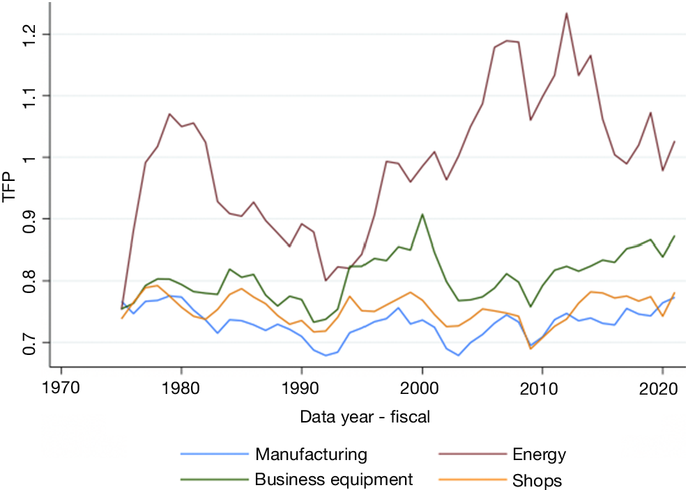
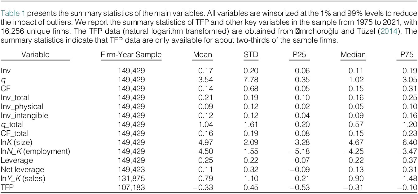
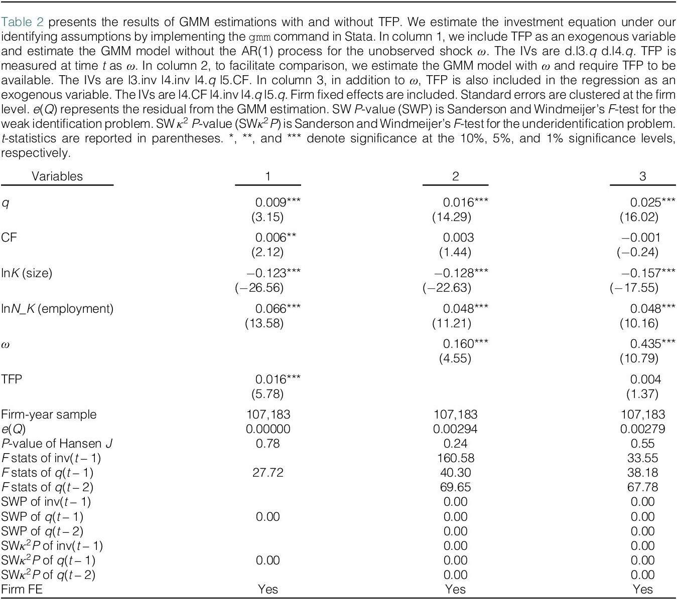
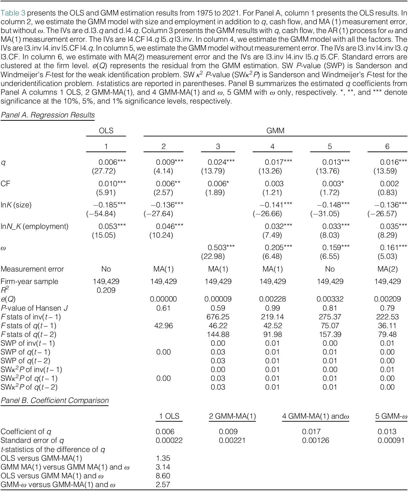

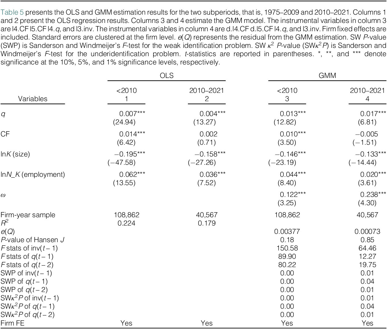

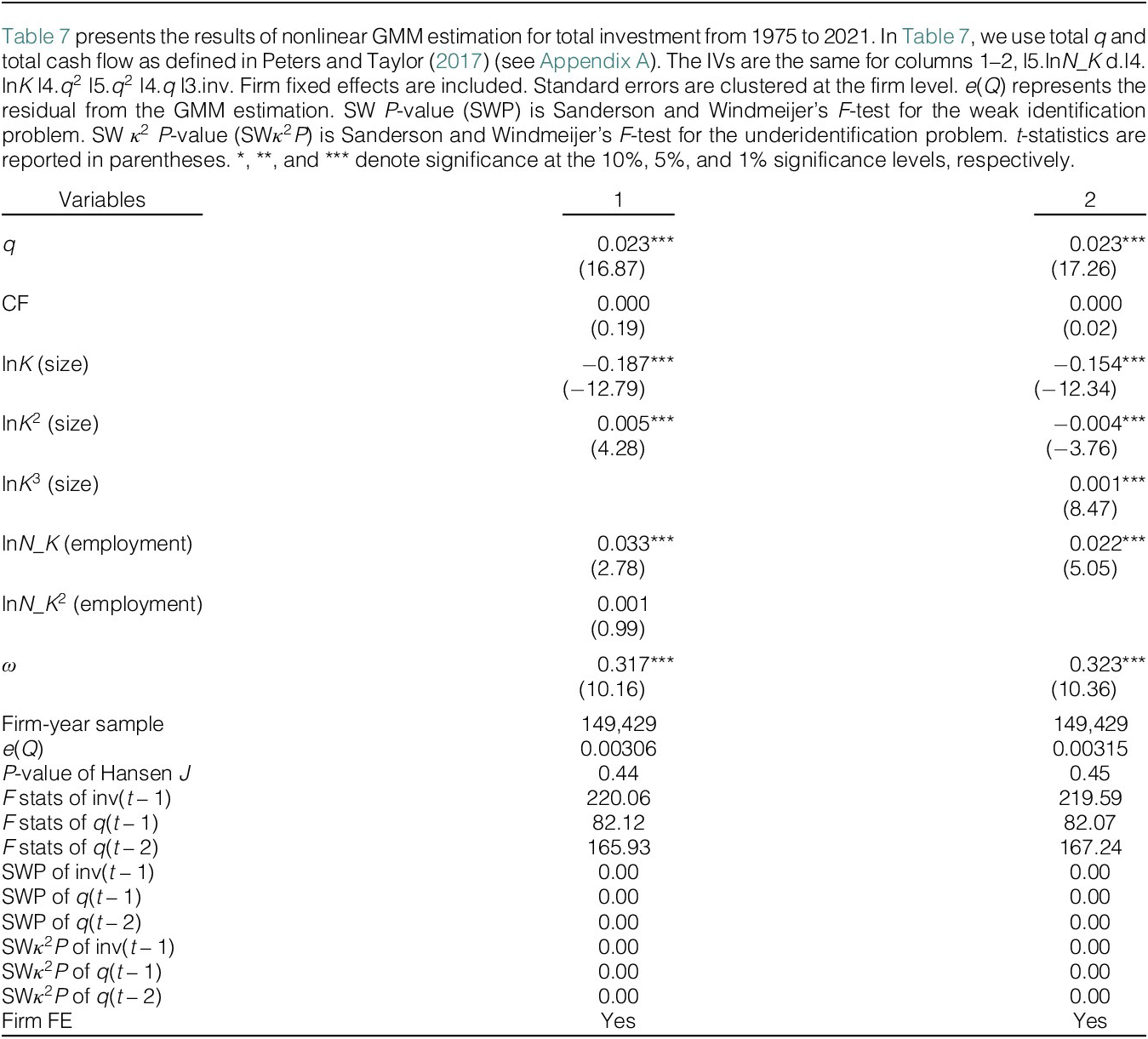


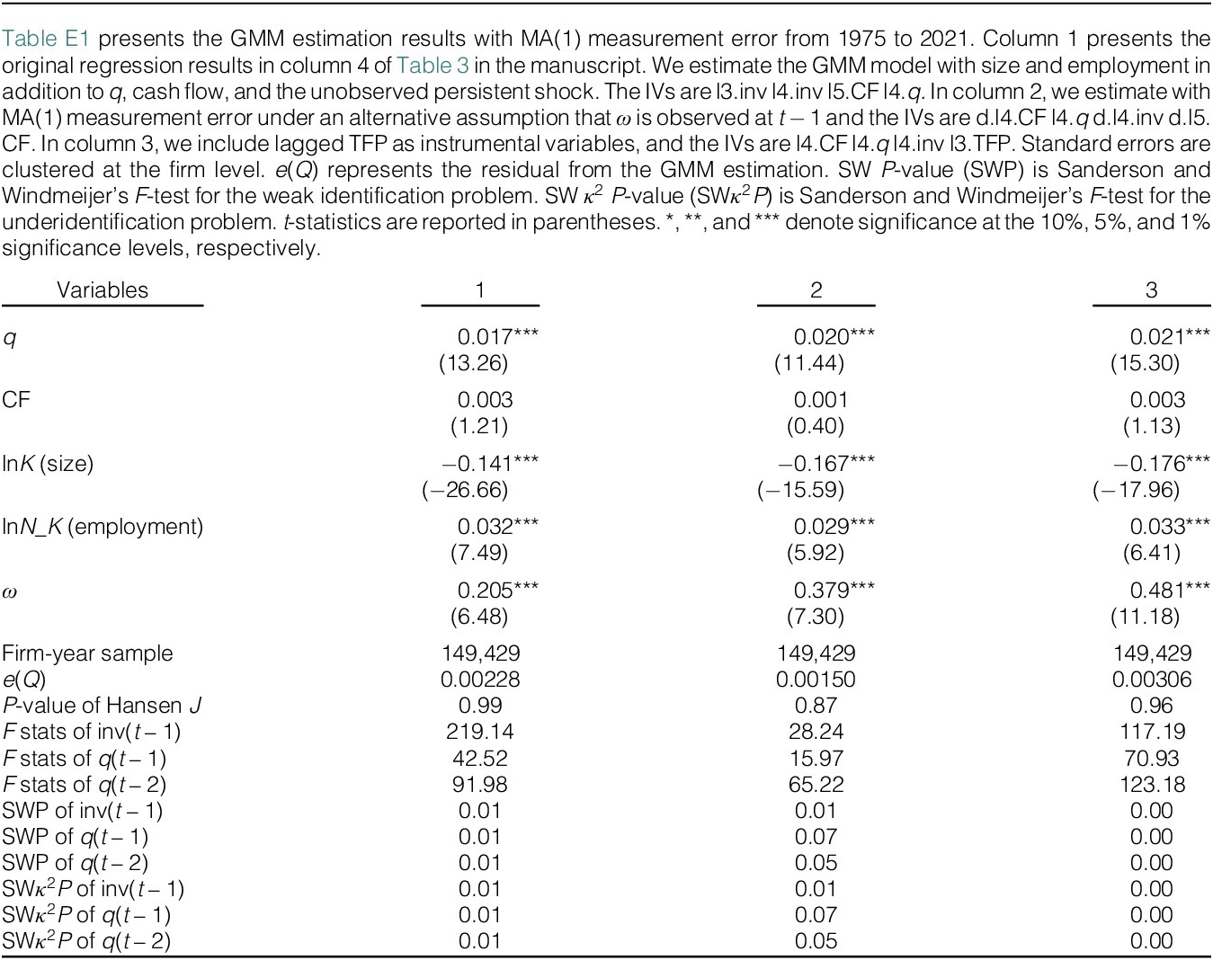


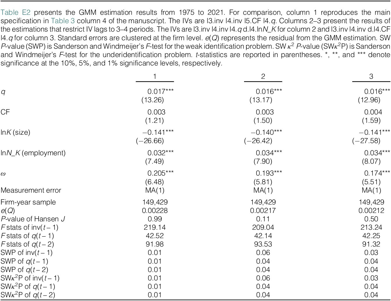


 Open access