


1 Introduction
Flow separation is one of the most intensively investigated problems in classical fluid mechanics (Goldstein Reference Goldstein1969). It occurs when the boundary layer loses contact with the associated confining wall, which is usually caused by a pressure gradient acting against the local flow direction (Simpson Reference Simpson1989). In many applications flow separation is an unwanted phenomenon, while in many others it has beneficial effects. Therefore, a detailed understanding of flow separation and the ability to control it have been the subject of many decades of research (Flatt Reference Flatt and Lachmann1961; Chang Reference Chang1976; Gad-el Hak & Bushnell Reference Gad-el Hak and Bushnell1991). Numerous control strategies exist to prevent separation, including streamlining of a flow body (Schlichting Reference Schlichting1951; Schubauer & Spangenberg Reference Schubauer and Spangenberg1960), boundary layer suction (Prandtl Reference Prandtl1935; Truckenbrodt Reference Truckenbrodt1956; Kametani et al. Reference Kametani, Fukagata, Örlü and Schlatter2015; Kornilov Reference Kornilov2015), injection of momentum into the boundary layer (Wallis & Stuart Reference Wallis and Stuart1958) and controlling separation by provoking it (Hurley Reference Hurley and Lachmann1961; Francis et al. Reference Francis, Keesee, Lang, Sparks and Sisson1979). In this paper we present observations that demonstrate – for the first time – that vertical flow separation over steep slopes in open channels may be suppressed by a lateral gradient in the streamwise velocity field upstream of the slope.
For a two-dimensional plane flow (for instance, the flow perpendicular to the axis of a wing profile or a slender body), the basic phenomenology of flow separation has been understood for a long time; a combination of a pressure gradient and bed shear stress determines the development of the boundary layer, and eventually whether or not it separates from the confining wall (Chang Reference Chang1970). For a larger deceleration of the flow, the pressure gradient acting against the flow direction increases and the likelihood of boundary layer separation increases (Schlichting Reference Schlichting1951). Flow control methods aim to either prevent separation or to reduce the size of the recirculation zone as much as possible (Chang Reference Chang1976). Therefore, much research effort has been dedicated to turbulent boundary layers and separation in two-dimensional plane flows (e.g. Clauser Reference Clauser1954; Stratford Reference Stratford1959; Simpson, Chew & Shivaprasad Reference Simpson, Chew and Shivaprasad1981; Nezu & Nakagawa Reference Nezu and Nakagawa1987; Simpson Reference Simpson1989, Reference Simpson1996; Scarano, Benocci & Riethmuller Reference Scarano, Benocci and Riethmuller1999), to understand the flow characteristics up to the separation point (Sandborn & Kline Reference Sandborn and Kline1961; Sandborn & Liu Reference Sandborn and Liu1968; Simpson et al. Reference Simpson, Chew and Shivaprasad1981) and in the recirculation zone after separation (Bradshaw & Wong Reference Bradshaw and Wong1972; Kim, Kline & Johnston Reference Kim, Kline and Johnston1980; Eaton & Johnston Reference Eaton and Johnston1981; Driver & Seegmiller Reference Driver and Seegmiller1985; Babarutsi, Ganoulis & Chu Reference Babarutsi, Ganoulis and Chu1989; Le, Moin & Kim Reference Le, Moin and Kim1997; Kourta, Thacker & Joussot Reference Kourta, Thacker and Joussot2015; Stella, Mazellier & Kourta Reference Stella, Mazellier and Kourta2017). Increase in computational power has made high-resolution numerical investigation of separation behaviour and control strategies an attractive addition (Dandois, Garnier & Sagaut Reference Dandois, Garnier and Sagaut2007; Garnier et al.. Reference Garnier, Pamart, Dandois and Sagaut2012; Zhang & Samtaney Reference Zhang and Samtaney2015; Alimi & Wünsch Reference Alimi and Wünsch2018). Several separation criteria have been proposed that are based on either the skin friction at the separation point (e.g. Cebeci Reference Cebeci1974), the pressure distribution in the free stream (e.g. Stratford Reference Stratford1959) or shape parameters that characterize the velocity profile in the boundary layer (e.g. Sandborn & Kline Reference Sandborn and Kline1961). It was shown by Cebeci, Mosinskis & Smith (Reference Cebeci, Mosinskis and Smith1972) that most of these methods were able to predict the location of the detachment point for steady two-dimensional flows with the reliability and accuracy needed for design purposes.
Definition of the different two-dimensional planes considered in this study. Sketched are the two-dimensional vertical  $xz$-plane (similar to the two-dimensional plane perpendicular to a wing profile) and the two-dimensional horizontal $xy$-plane. The bed topography causing vertical separation phenomena in the two-dimensional vertical plane may result from local erosion downstream of a hydraulic structure.
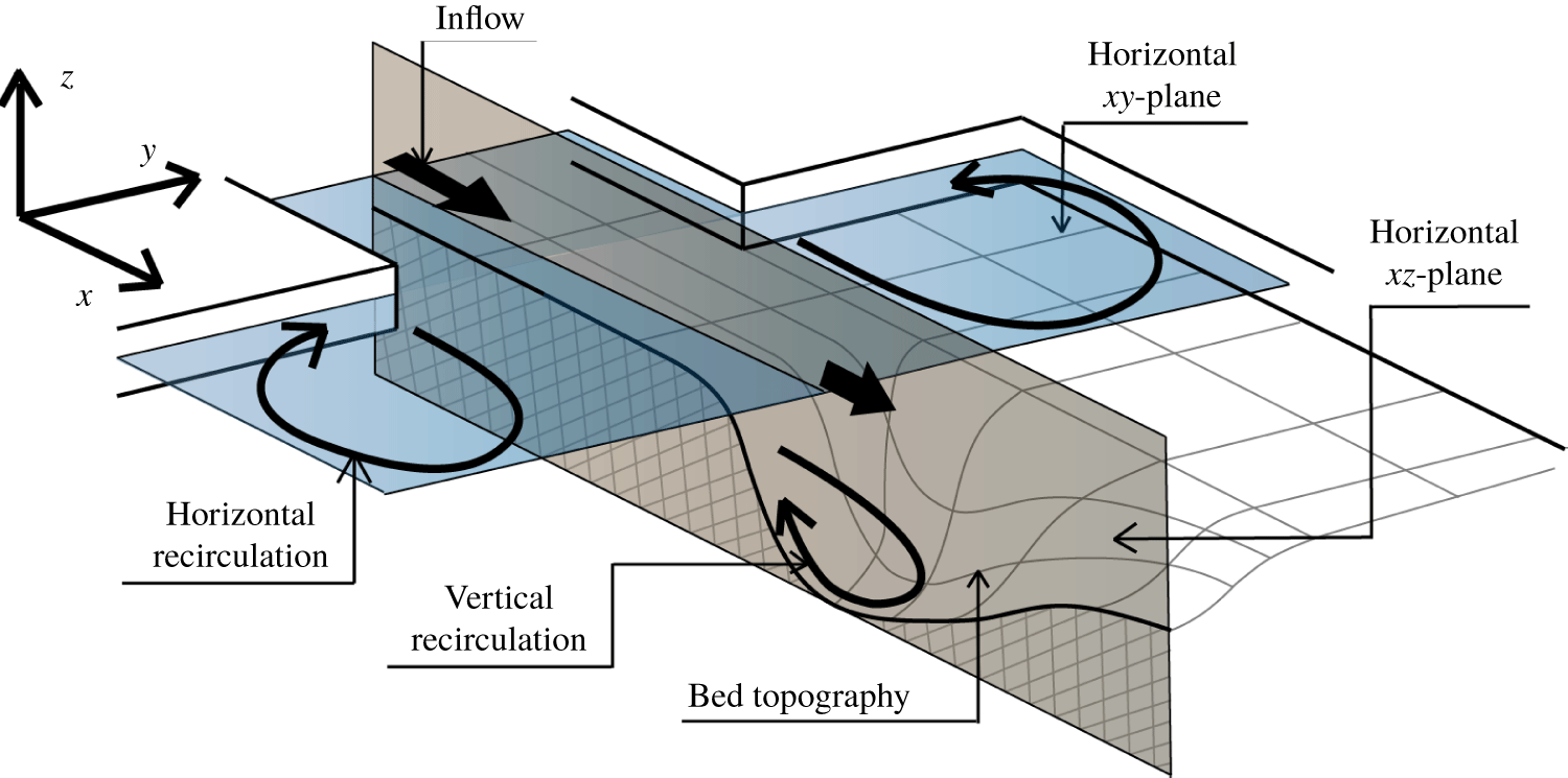
In this paper we study flow separation phenomena in open channel flows. A distinction needs to be made between boundary layer separation in the two-dimensional (2-D) vertical plane and in the 2-D horizontal plane (for an illustration, see figure 1). In the 2-D vertical plane, the bed topography is the major cause of flow separation, while in the 2-D horizontal plane, the plan form or the presence of hydraulic structures are determining factors. In both the 2-D horizontal and the 2-D vertical planes, flow separation phenomena are comparable, although there are some differences. In the 2-D horizontal plane, bed friction may play an important role in determining the extent of the horizontal recirculation zone after separation (Babarutsi et al. Reference Babarutsi, Ganoulis and Chu1989). This is, for instance, the case when the flow can be considered shallow, that is, when the horizontal length scales of the flow are much larger than the flow depth (Uijttewaal Reference Uijttewaal2014). The flow can be considered 2-D vertical if variations in the lateral direction of the domain are small.
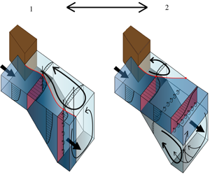
In reality, flow is not two-dimensional but three-dimensional, and the inclusion of the third dimension largely complicates the situation due to the extra degrees of freedom (Tobak & Peak Reference Tobak and Peak1982; Simpson Reference Simpson1996; Cherry, Elkins & Eaton Reference Cherry, Elkins and Eaton2008; Gao et al. Reference Gao, Ma, Zambonini, Boudet, Ottavy, Lu and Shao2015). Field observations of a flow with large lateral gradients in the streamwise velocity over a bed topography similar to that of figure 1, revealed complex separation phenomena (Broekema, Labeur & Uijttewaal Reference Broekema, Labeur and Uijttewaal2018). For sufficiently large lateral gradients of the streamwise velocity, vertical flow separation did not occur, whereas it was observed if the lateral variation of the mean flow field was limited. Moreover, the flow velocity at the deepest point of the topography, as sketched in figure 1, was found to depend significantly on the upstream flow conditions. These observations exemplify the important role of upstream variability of the flow field in engineering applications, which motivated the present study. The observed phenomena from the field are investigated experimentally for a highly simplified geometry. In the experiment, a horizontally non-uniform flow over a downstream bed slope was investigated. The primary aim of the experiment was to verify to which extent lateral non-uniformity of the upstream horizontal flow field influences vertical flow separation at the slope, and the corresponding flow fields on top of and downstream of the slope. A secondary aim was to assess any potential impact of whether or not vertical flow separation occurs on the hydraulic loading on the confining boundary. The present study did not pursue new flow control strategies, however, the results may serve as an inspiration for that particular purpose.
In the paper, first, the approach followed with the experimental work is described in § 2. In § 3 time-averaged and depth-averaged flow fields are presented, as well as the derived bed shear stresses. These observations form the basis for a further analysis and characterization of the flow in § 4. We reflect upon the findings and their relevance in § 5.
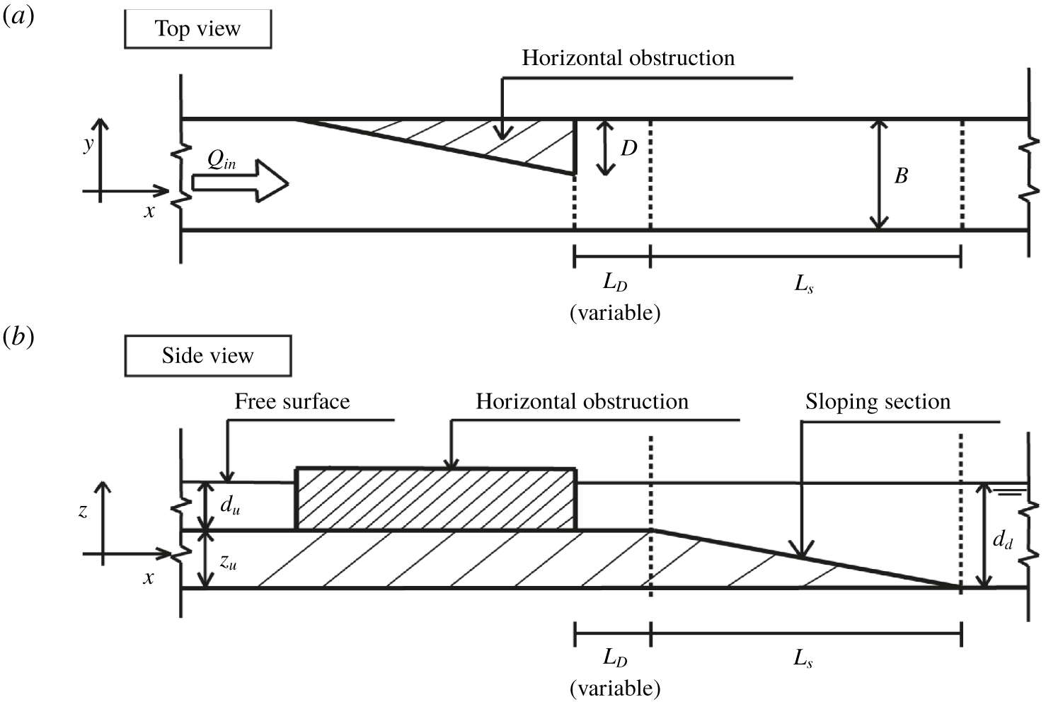
Sketch of the experimental configuration. (a) Top view of the experimental set-up. The flume width  $B$ is 0.4 m, and the horizontal contraction has a maximum width $D$ of 0.5 $B$. The streamwise distance of the horizontal contraction to the upstream edge of the slope $L_{D}$ is an experimental variable to control the magnitude of the lateral velocity gradient at the slope. The length of the sloping section $L_{s}$ is determined by the slope steepness $i_{b}$, which is an experimental variable as well. (b) Side view of the set-up. The water depth upstream of the slope is given by $d_{u}=0.12~\text{m}$, and the water depth downstream of the slope is given by $d_{d}=0.27~\text{m}$. The height of the false bed $z_{u}$ is 0.15 m.
2 Methodology
2.1 Experimental set-up
The experimental work was conducted in a 14 m long, 0.4 m deep and 0.4 m wide glass-sided flume (figure 2). Broekema et al. (Reference Broekema, Labeur and Uijttewaal2018) related the suppression of vertical flow separation to the magnitude of the lateral velocity gradient, which is therefore an important variable in the experiment. The lateral non-uniformity in the streamwise velocity was imposed by an obstruction on one side of the flume, located upstream of the slope, with a maximum lateral blockage of half the flume width. The relative shallowness of the flow is considered an important driver of the phenomena, motivating the choice for a one-sided (asymmetrical) obstruction which uses the available flume width more optimally in this respect than a two-sided (symmetrical) set-up. Moreover, a symmetrical expansion tends to downstream flow attachment, favouring one side of the domain (e.g. Kantoush & Schleiss Reference Kantoush and Schleiss2009), which would leave the interpretation of the results ambiguous. For similar reasons, previous studies concerning a lateral expansion over a flat bed (van Prooijen, Battjes & Uijttewaal Reference van Prooijen, Battjes and Uijttewaal2005; Talstra Reference Talstra2011) also used a one-sided obstruction, which enables a direct comparison of the results of the present study with their findings.
The mixing layer caused by the abrupt expansion downstream of the obstruction develops over a certain streamwise distance towards the slope. As it develops, the width of the mixing layer increases while the velocity difference across the mixing layer decreases (van Prooijen & Uijttewaal Reference van Prooijen and Uijttewaal2002), giving a reduction of the lateral velocity gradient. Thus, by varying the (streamwise) distance  $L_{D}$ from the horizontal obstruction to the upstream edge of the slope, the magnitude of the lateral velocity gradient at the upstream edge of the slope is controlled. Another important experimental variable is the slope steepness $i_{b}$, which was selected such that vertical flow separation would occur for a horizontally uniform flow (so for a 2-D vertical situation). It was verified whether or not this was the case before putting the horizontal obstruction in the flume. For all slopes that we tested in the experiment, vertical flow separation was observed in the 2-D vertical case.
Upstream of the slope, a false bed with a height  $z_{u}$ of 0.15 m was placed in the flume. The false bed was positioned directly at the inlet of the flume and had a length of 8 m to ensure a fully developed flow at the upstream edge of the lateral obstruction. The bed level in the flume was uniform in the lateral direction. The upstream water depth, $d_{u}$, was approximately 0.12 m, and the downstream water depth, $d_{d}$, approximately 0.27 m. These values were chosen to achieve an increase in flow depth which is the same as in the field case considered in Broekema et al. (Reference Broekema, Labeur and Uijttewaal2018). The discharge $Q_{in}$ was chosen such that the maximum Froude number $Fr=0.4$, which is sufficiently low to minimize the effects of surface disturbances, and that the Reynolds number $Re=3\times 10^{4}$, which is sufficiently high to ensure that the flow is fully turbulent.
Velocity and turbulence were measured using a Nortek Vectrino+ acoustic Doppler velocimeter (Nortek AS, Rud, Norway). A sideward-looking probe was used to measure close to the bed, at a height of 0.6 cm. Local interference of the probe with the flow at the sampling location is avoided as velocities are measured at a horizontal distance of 5 cm away from the probe. To obtain a high quality signal, the flow was locally seeded with tiny ( ${\approx}30~\unicode[STIX]{x03BC}\text{m}$) hydrogen bubbles generated by electrolysis using 0.1 mm platina wires. The velocimeter was used with a sampling rate of 25 Hz, and the accuracy of the velocity measurements is $\pm 0.5\,\%$. For each experimental case velocities were measured at a large number of positions in the domain. At each horizontal position, the velocimeter was deployed at five different vertical positions; as close to the bed as possible (0.6 cm), 1.6 cm above the bed, 2.6 cm above the bed, at half the water depth and 1 cm below the free surface. At each measurement position a time series of the flow velocity of three minutes was sampled to have statistically significant turbulence characteristics and to be able to sufficiently average out the turbulence to determine the mean flow field.
2.2 Experimental cases
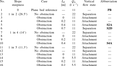
By systematically varying the slope steepness and the distance from the obstruction to the upstream edge of the slope, the influence of the upstream flow field on the flow field at the slope was assessed. Beforehand, we did not know for which cases, if any, vertical flow separation would not occur. Therefore, a large number of different experiments were performed. In table 1 an overview of all experimental runs is given, each with their relevant characteristics. This paper focuses on a select number of cases (indicated in table 1 in the rightmost column) that revealed the principal phenomena; the transition between a vertically separating and an attaching flow state, and the scaling of the flow structure with the relative increase in depth.
In almost all investigated cases with lateral non-uniformity, the flow stayed attached to the slope whereas it separated from the slope for the laterally uniform case. This is a feature that was not intuitively expected beforehand. In supplementary movie 1 (available at https://doi.org/10.1017/jfm.2019.972) this is demonstrated for the 1 in 2 slope. Vertical flow separation was clearly observed after systematically moving the horizontal obstruction further upstream from the edge of the slope. This supports the idea from Broekema et al. (Reference Broekema, Labeur and Uijttewaal2018) that the occurrence of the phenomena depends on the magnitude of the lateral gradient in streamwise velocity. For all cases investigated, changing the discharge did not have a significant impact on the observed flow patterns. Provided the Froude number is lower than 1, the phenomena scale well with the velocity.
In the supplementary material, the measured three-dimensional time-averaged flow fields covering the entire parameter space of the experiments are provided, which demonstrate the consistency of these observations. The remainder of this study will highlight four of these cases:
(i) a plane bed mixing layer, which serves as a reference case (PB);
(ii) a horizontal mixing layer over a 1 in 2 slope that attaches to the slope (S2A);
(iii) a horizontal mixing layer over a 1 in 2 slope that detaches from the slope (S2D);
(iv) a horizontal mixing layer over a 1 in 4 slope that attaches to the slope (S4A).
Cases S2A and S2D demonstrate the influence of the upstream flow field on the occurrence of, respectively, vertical attachment and separation at the slope. Cases S2A and S4A demonstrate the effect of the slope steepness on the flow field in case of vertical attachment.
Overview of the different experimental runs that were performed in this study. In the remainder, the focus is on the select number of cases indicated in bold: case PB (plane bed mixing layer, reference), S2A (mixing layer over a 1 in 2 slope that stays attached to the bed), S2D (mixing layer over a 1 in 2 slope that detaches from the bed) and S4A (mixing layer over a 1 in 4 slope that stays attached to the bed).
2.3 Flow data processing
Prior to analysis, the measured time series were despiked following a two-step strategy: first, the data spikes due to moments of low seeding in front of the velocimeter were detected and replaced using a Hampel filter (Pearson et al. Reference Pearson, Neuvo, Astola and Gabbouj2016). These spikes tend to be grouped in time (MacVicar & Best Reference MacVicar and Best2013). The Hampel filter was applied in such a way as to discard observed velocities that are farther than ten standard deviations away from the mean velocity. As a second step, data were despiked using the phase-space algorithm of Goring & Nikora (Reference Goring and Nikora2002). Despiking with this algorithm detects and replaces those data spikes that are randomly distributed.
After despiking of the measured time series, a Reynolds decomposition was applied to the velocity signal as follows:
 $$\begin{eqnarray}u_{i}=\overline{u}_{i}+u_{i}^{\prime },\end{eqnarray}$$
 where  $u_{i}$, with $i=1,2,3$, are velocity components in the $x,y,z$ directions, respectively. The overbar denotes a time average and the prime denotes the fluctuating component of a quantity. The time-averaged velocity is for instance defined as
 $$\begin{eqnarray}\overline{u}_{i}(x,y,z)=\frac{1}{T}\int _{0}^{T}u_{i}(x,y,z,t)\,\text{d}t,\end{eqnarray}$$
 in which  $T$ is the total measuring time. Using (2.1) the Reynolds shear stress components, defined as $\unicode[STIX]{x1D70F}_{ij}^{\prime }=-\unicode[STIX]{x1D70C}\overline{u_{i}^{\prime }u_{j}^{\prime }}$, are straightforwardly calculated.
For a number of cases the mean vertical structure of the flow is rather uniform, motivating the consideration of time- and depth-averaged quantities. Depth averaging of the mean velocities is performed component-wise, as follows:
 $$\begin{eqnarray}U_{i}(x,y)=\frac{1}{d}\int _{z_{0}}^{\unicode[STIX]{x1D702}}\overline{u}_{i}(x,y,z)\,\text{d}z,\end{eqnarray}$$
 in which  $U_{i}$, with $i=1,2$, are the time- and depth-averaged velocity components in the $x$ and $y$ directions, respectively, $z_{0}$ is the local bed level, $\unicode[STIX]{x1D702}$ is the local water surface level and $d=\unicode[STIX]{x1D702}-z_{b}$ is the local water depth. To calculate the integral in (2.3), velocities were assumed zero at the bed and linearly interpolated up to the first measurement point (0.6 cm above the bed), and velocities at the surface level were assumed to have the same value as at the first measurement position below the surface (1 cm below the surface).
For visualization purposes, time-averaged velocity data are projected onto a spatial grid with interval lengths of  $\unicode[STIX]{x0394}x=0.025~\text{m}$, $\unicode[STIX]{x0394}y=0.0125~\text{m}$ and $\unicode[STIX]{x0394}z=0.01~\text{m}$. For the depth-averaged mean flow fields the step sizes $\unicode[STIX]{x0394}x$ and $\unicode[STIX]{x0394}y$ of the horizontal grid are the same as used for the time-averaged flow fields.
2.4 Scaling
Three different horizontal length scales play an important role in characterizing the flow field. First, leeward of the obstruction, a horizontal recirculation zone develops and previous studies have shown the dependency of the extent of the horizontal recirculation zone on the width of the lateral expansion,  $D$. Second, at the interface between the main flow and the horizontal recirculation zone, a mixing layer develops. According to Chu & Babarutsi (Reference Chu and Babarutsi1988) the development of the horizontal mixing layer can be scaled using a length scale $L_{f}=d/c_{f}$, where $c_{f}$ is the bed friction coefficient. The bed friction coefficient relates to the bed shear stress $\unicode[STIX]{x1D70F}_{b}$ through $\unicode[STIX]{x1D70F}_{b}=\unicode[STIX]{x1D70C}c_{f}U^{2}$. Third, in case the flow stays attached to the bed, the flow field at the slope depends on the relative increase in depth. This introduces a horizontal length scale over which the increase in flow depth takes place, defined as $L_{s}=i_{b}\unicode[STIX]{x0394}d$, where $\unicode[STIX]{x0394}d$ is the increment of the flow depth at the slope. For the experimental conditions, the order of magnitude of the friction length scale $L_{f}\approx O(10^{1})$ m, whereas the orders of magnitude of the expansion width and the depth scale are $D\approx L_{s}\approx O(10^{-1})$ m. Therefore, the flow field in the area of interest is mainly dependent on the expansion width and the bed slope, with a limited role of bed friction. In line with previous studies into laterally expanding flows and horizontal recirculation zones (Chu & Babarutsi Reference Chu and Babarutsi1988; Babarutsi et al. Reference Babarutsi, Ganoulis and Chu1989; Talstra Reference Talstra2011), the $x$-coordinate is scaled with the expansion width $D$. The trailing edge of the horizontal obstruction is defined as the origin ( $x/D=0$).
At the sloping section a different scaling is more appropriate. For a close analysis of the dependency of the flow field on the slope steepness, the  $x$-coordinate is scaled with the length of the slope, $L_{s}$. This scaling is only appropriate at the sloping section itself; it has no physical meaning in the rest of the domain. Given the dependency of the phenomena on the relative increase in depth, the vertical $z$-coordinate is scaled with the upstream water depth $d_{u}$.
3 Experimental observations
Contracting the flow horizontally led to suppression of vertical flow separation in nearly all the cases investigated in this experimental set-up (see table 1). In this section, the observed flow fields from the selected experimental cases are presented. First, the flow fields of a vertically attaching (case S2A) and separating (case S2D) laterally non-uniform flow are compared. Next, to demonstrate the influence of vertical separation on the horizontal flow pattern, depth-averaged flow fields are presented and compared. Finally, bed shear stress measurements are shown, which is motivated by the influence of flow attachment or separation on the hydraulic loads on the slope. The differences in hydraulic loading justify a further classification and a deeper analysis of the flow at the slope.
3.1 Time-averaged flow
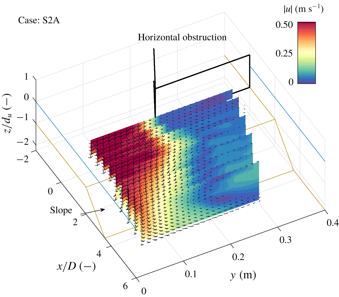
Interpolated three-dimensional, time-averaged flow field of a laterally non-uniform flow that stays attached to the bed (case S2A). The colour bar denotes the magnitude of the mean velocity  $|\overline{u}|=\sqrt{\overline{u}_{1}^{2}+\overline{u}_{2}^{2}+\overline{u}_{3}^{2}}$. The brown lines show the bathymetry in the flume, the bold black lines mark the horizontal obstruction and the blue lines indicate the water level. The vertical axis is scaled using the upstream water depth $d_{u}$. The downstream end of the obstruction is chosen as the origin $x/D=0$.
Interpolated three-dimensional, time-averaged flow field of a laterally non-uniform flow that separates from the bed (case S2D). The colour bar denotes the magnitude of the mean velocity  $|\overline{u}|=\sqrt{\overline{u}_{1}^{2}+\overline{u}_{2}^{2}+\overline{u}_{3}^{2}}$. The brown lines show the bathymetry in the flume, the bold black lines mark the horizontal contraction and the blue lines indicate the water level. The vertical axis is scaled using the upstream water depth $d_{u}$. The downstream end of the obstruction is chosen as the origin $x/D=0$.
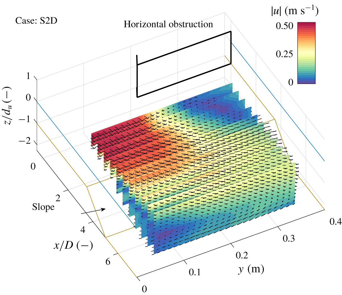
The three-dimensional, time-averaged flow field of a horizontal mixing layer that stays attached to the bed (case S2A) is compared to that of a mixing layer that separates from the bed (case S2D). The latter was the only laterally non-uniform case where clear vertical flow separation was observed. Figures 3 and 4 show the flow field of case S2A (vertically attached flow) and case S2D (vertically separated flow), respectively.
In both cases, the flow separates from the trailing edge of the obstruction with a large horizontal recirculation zone in the lee of the obstruction, which has been observed for similar configurations over a flat bed in previous experiments (Babarutsi et al. Reference Babarutsi, Ganoulis and Chu1989; Talstra Reference Talstra2011). In the current configuration, which includes a slope, the extent of the horizontal recirculation zone also depends on the vertical structure of the flow at the slope. A strong convergence of the flow towards the high-velocity side is observed when the flow stays attached to the slope (S2A, figure 3), whereas the flow strongly diverges when it separates from the bed (S2D, figure 4). For both cases, between the main flow and the recirculation zone a turbulent horizontal mixing layer develops (Brown & Roshko Reference Brown and Roshko1974). Initially, the horizontal mixing layer development of both cases is similar, but at the slope they start to differ. It will be shown in § 4.2 that there are strong similarities between this mixing layer and the flat bed mixing layers observed in previous experiments of van Prooijen & Uijttewaal (Reference van Prooijen and Uijttewaal2002) and Talstra (Reference Talstra2011). For both cases S2A and S2D a secondary circulation (in the  $yz$-plane) is observed, but of opposite sign. This behaviour is consistent across the investigated parameter range (see table 1), as evidenced by the corresponding three-dimensional time-averaged flow fields shown in the supplementary material.
Horizontal flow fields of case S2D (vertical flow separation, slope 1 in 2). Magnitude of mean horizontal velocity  $|\overline{u}_{h}|=\sqrt{\overline{u}_{1}^{2}+\overline{u}_{2}^{2}}$, and streamlines in a horizontal plane near (a) the surface and (b) near the bed. The obstruction is located at a distance of 3.5 $D$ from the slope. The upstream and downstream edge of the slope are indicated by the black dashed lines. The location of the contraction is plotted with solid black lines. The red dots denote measurement locations.
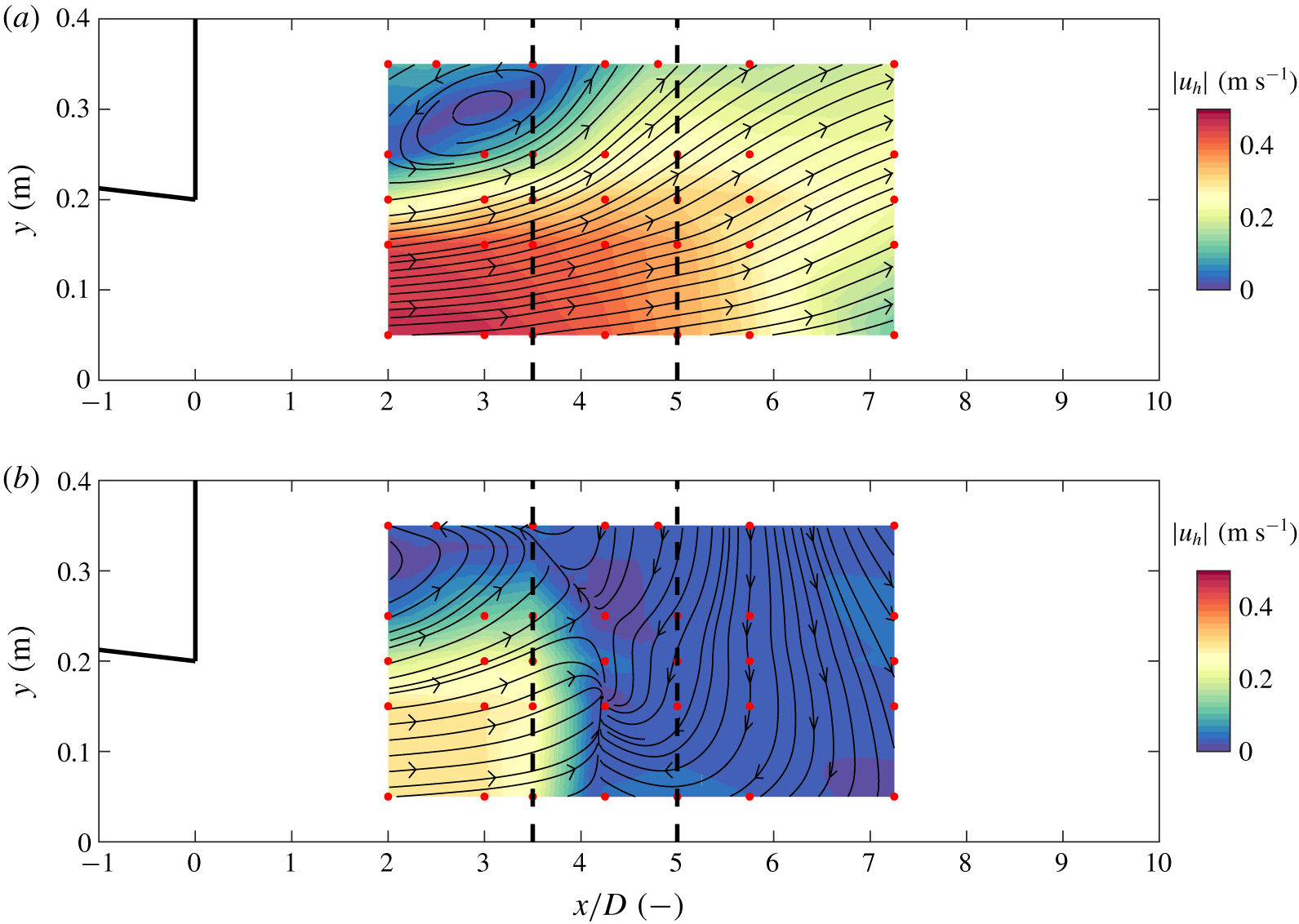
When the flow stays attached to the bed, the vertical structure of the flow is rather uniform. For the vertically separating case, the flow is mainly confined to the upper part of the water column. This is shown for case S2D in figure 5, where the horizontal flow field in the top layer of the water column (figure 5a) and the horizontal flow field near the bed (figure 5b) are compared. The near-bed flow differs significantly from the near-surface flow, the latter showing similarity to a plane bed laterally expanding flow (Babarutsi et al. Reference Babarutsi, Ganoulis and Chu1989). For case S2D, the general features of such flows characterize the flow in the top part of the water column with a flow depth of approximately the upstream depth  $d_{u}$.
For case S2D, vertical flow separation was finally observed after systematically moving the contraction further away from the upstream edge of the slope. For a certain distance, an abrupt transition between the two flow states was observed; a very small change of the position of the contraction caused the flow to transform from one state into the other. Furthermore, it was observed that the flow over the slope changed from one state into the other, without changing the position of the contraction, also showing that the transition is reversible. Although it is unclear what caused this change, it is additional evidence (although slightly circumstantial) that the transition between the flow states may be a bifurcation type of mechanism.
3.2 Depth-averaged flow
As was shown in § 3.1, the vertical structure is rather uniform if the flow stays attached to the bed, motivating analyses of the depth-averaged flow fields of cases S2A and S4A. The influence of the slope on the horizontal flow field is shown by comparing the corresponding depth-averaged flow fields to those of the reference plane bed case (PB).
In figure 6 the depth-averaged flow fields of case PB (plane bed reference case, figure 6a), case S2A (slope 1 in 2, attached, figure 6b), case S4A (slope 1 in 4, attached, figure 6c) and case S2D (slope 1 in 2, separation, figure 6d) are shown. Although the flow field of case S2D is non-uniform over the vertical, the depth-averaged flow field of this case is shown here as well for completeness.
Interpolated mean depth-averaged horizontal flow fields for cases PB (a), S2A (b), S4A (c) and S2D (d). The colour bar denotes the magnitude of the mean depth-averaged horizontal velocity  $|U|=\sqrt{U_{1}^{2}+U_{2}^{2}}$, the solid black lines indicate the location of the horizontal contraction and the red dots mark the measurement positions. In panels (b–d) the position of the slope is indicated with black dashed lines.
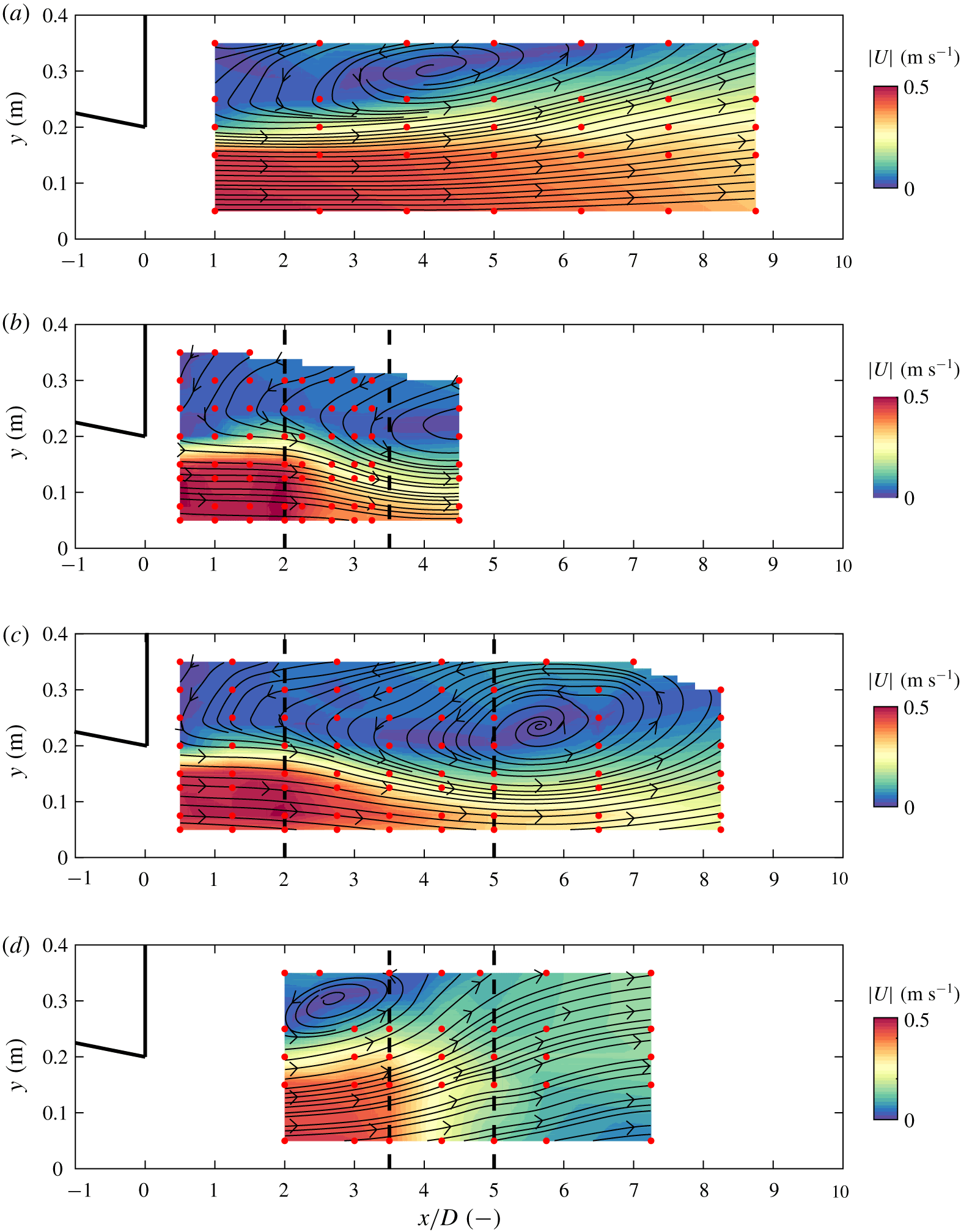
The horizontal flow field observed at the plane bed reference case (case PB) shows a streamwise extent of the horizontal recirculation zone of approximately eight times the expansion width  $D$. The core of the recirculation zone is located at a distance 3.5–4 times $D$ from the detachment point. The velocity difference between the high-velocity side and the low-velocity side reduces with streamwise distance, and the mixing layer centreline position displaces towards the low-velocity side. This is consistent with observations from previous experiments of Babarutsi et al. (Reference Babarutsi, Ganoulis and Chu1989), Talstra (Reference Talstra2011) and van Prooijen & Uijttewaal (Reference van Prooijen and Uijttewaal2002);
In both case S2A (figure 6b) and case S4A (figure 6c) the lateral extent of the recirculation zone is much larger than for case PB. For these two cases the streamlines in the conveying part of the flow converge, with a maximum just after the toe of the slope. For both case S2A and case S4A the flow velocities at the toe of the slope are similar. This raises the idea that the depth-averaged horizontal flow field of a mixing layer that stays attached to the bed over a sloping section depends on the relative increase in depth, rather than on the bed slope  $i_{b}$. This will be further investigated in § 4.2.
For case S2D (figure 6d) a horizontal recirculation zone is still recognized, but of much smaller size than for cases PB, S2A and S4A. The main flow diverges and thus the velocity difference over the mixing layer reduces at the slope. Although for case S2D the vertical velocity profile is far from uniform (figure 5), horizontal mixing layer behaviour is still observed in the depth-averaged flow field.
3.3 Bed shear stress
The influence of flow attachment and separation on the hydraulic load on the bed is assessed by comparing the bed shear stresses for the selected cases. The bed shear stress was not measured directly, but derived from the velocity observations. For a flow over a horizontal bed, a good estimate of the bed shear stress is provided by the vertical component of the observed Reynolds stress tensor,  $\unicode[STIX]{x1D70F}_{xz}$, near the bed (Kim et al. Reference Kim, Friedrichs, Maa and Wright2000; Guan et al. Reference Guan, Melville and Friedrich2014).
For the sloping bed cases of this study, this approach is slightly adapted in that the Reynolds stress tensor is multiplied first with the unit normal vector at the bed. The bed shear stress  $\unicode[STIX]{x1D70F}_{b}$ is then derived as the magnitude of the tangential component of the resulting stress vector. According to Biron et al. (Reference Biron, Robson, Lapointe and Gaskin2004), interference of the velocity signal due to the wall is negligible at distances from the wall of more than approximately 10 % of the flow depth. Accordingly, at every horizontal measurement position we chose the vertical sampling point closest to this optimal location to derive the bed shear stress. The corresponding distances to the wall vary between 8 % and 13 % of the flow local depths which, considering he above criterion, is an acceptable range.
Bed shear stress for cases PB (black), S2A (blue), S4A (red) and S2D (grey). The black dotted lines and the annotations in the figure denote the respective locations of the bed slope in the domain for the sloping cases.
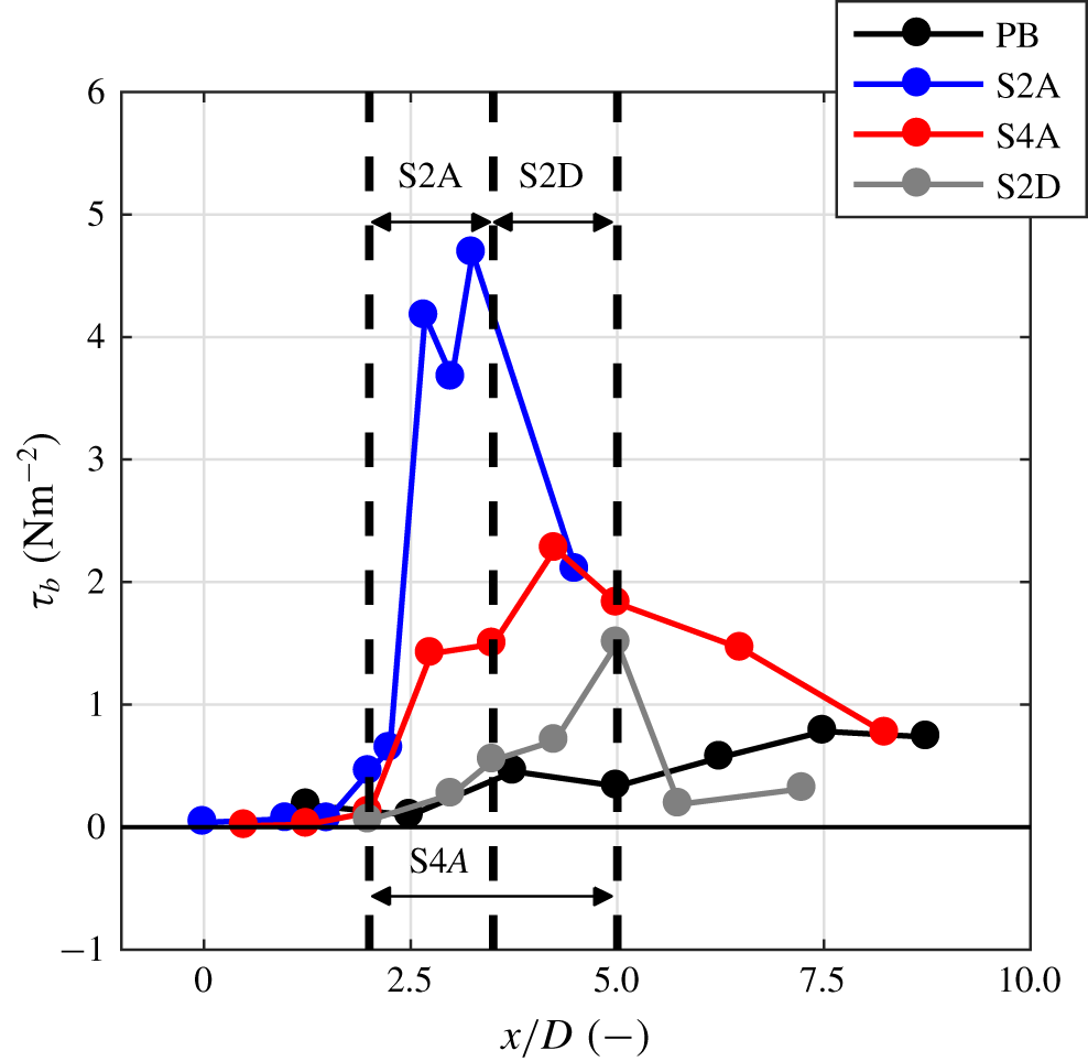
Figure 7 shows calculated values of  $\unicode[STIX]{x1D70F}_{b}$ for all considered cases. Up until the upstream edge of the slope, the bed shear stresses are similar for all cases. It is clear from figure 7 that the flow attachment at the bed slope leads to much larger bed shear stresses than flow separation at the slope. The corresponding increase of the bed shear stress is, in case of vertical attachment, furthermore dependent on the steepness of the slope; this is illustrated by case S2A for which the magnitude of the occurring bed shear stress is significantly larger than for case S4A. For case S2D the bed shear stress peaks at the downstream end of the slope, which could indicate reattachment of the flow at that position.
Another consequence of the flow staying attached is that there is (especially for the steeper slopes) a strong curvature of the streamlines around the edge of the slope. Therefore, one may expect the pressure to locally deviate from a hydrostatic pressure distribution, which changes the form drag exerted by the flow on the slope. This combination of horizontal convergence and suppression of vertical flow separation has thus potentially large consequences for the hydraulic loading. Therefore, it is important to fully understand the conditions that determine the transition between a separating and attached flow state. To this end, in the remainder of this paper, the dynamics of the different observed flow states will be closely analysed and characterized.
4 Analysis and characterization of the flow
The observations demonstrated that there are two different flow states possible at the slope in the flume; (i) a combination of vertical flow attachment and horizontal convergence, and (ii) a combination of vertical flow separation and horizontal divergence. In this section, these states are further characterized to understand key differences between their associated dynamics. First, a conceptualization of the two different flow states is given in § 4.1. Next, the horizontal mixing layer for both flow states is analysed. Finally, the pressure field and total energy head are investigated.
4.1 Flow states
Figure 8 shows a conceptual sketch of the respective flow states that were observed during the experiment. The transition between the two flow states behaves as an unstable bifurcation. For the sketched upstream flow condition, the flow may redistribute in two different ways, as indicated by the red cross-sections in the figure. When vertical flow separation is suppressed, the conveyance cross-section elongates vertically and compresses horizontally. The development of the horizontal mixing layer is closely analysed in § 4.2.1. Due to the combination of vertical flow attachment and convergence, the deceleration of the flow on the high-velocity side of the mixing layer is less than what would be expected based on mass conservation in the 2-D vertical plane. The presence of the slope intensifies turbulence (§ 4.2.2). This may influence the growth of large turbulent structures.
Conceptual visualization of the two different observed flow structures in the flume experiment: (a) a flow that stays attached to the bed and converges in the horizontal plane; (b) a flow that separates from the bed and diverges in the horizontal plane. In both cases, the velocity averaged over the flume cross-section reduces proportionally to the increase in cross-section, but in (a) the bulk of the flow (red cross-section) is distributed over the vertical whereas in (b) the bulk of the flow is distributed over the horizontal. The red line denotes the interface between the main flow and the horizontal recirculation zone.

If the flow detaches from the bed, for a short streamwise distance the conveyance cross-section remains more or less the same vertically and it stretches horizontally (flow state 2). At the interface between the conveyance cross-section and the vertical recirculation, energy dissipation is larger than at a smooth plane bed (§ 4.3), and as a result, the streamwise extent of the horizontal recirculation zone is shorter. This behaviour is analogous to a horizontal plane bed mixing layer over a rougher bed. Over the relatively short distance of the slope, horizontal mixing layer behaviour was recognized in the conveyance cross-section of case S2D. As will be shown in §§ 4.2 and 4.3, downstream of the slope the mixing layer structure has largely disappeared due to the vertical mixing. For reasons yet unclear, for this flow state the upstream flow conditions are no longer sufficient to suppress vertical flow separation at the slope.
4.2 Horizontal mixing layer dynamics
In this section the horizontal mixing layer is analysed to assess the influence of the slope on the mixing layer dynamics for the selected cases. First, the mean flow field is analysed; self-similarity of the dynamics and differences in mixing layer development are shown. Second, turbulence properties are shown for the selected cases.
4.2.1 Mixing layer development
We assess the self-similar behaviour of the mean flow field of the horizontal mixing layer. A theoretical model for the development of a mixing layer at the interface of two uniform flows without interference of the sidewalls was developed by van Prooijen & Uijttewaal (Reference van Prooijen and Uijttewaal2002), assuming self-similarity of the lateral profiles of the depth-averaged streamwise velocity. Talstra (Reference Talstra2011) has shown that the self-similar behaviour of the horizontal mixing layer in the case of a lateral expansion compares well to the theoretical model of van Prooijen in the near field and the middle field ( $x/D<4$). The current experiment combines a lateral expansion with a downstream increase in flow depth, and the distance from the horizontal obstruction to the downstream edge of the slope in general falls within the range of $x/D<4$. We therefore fit the depth-averaged velocity to the proposed shape function of van Prooijen & Uijttewaal (Reference van Prooijen and Uijttewaal2002):
 $$\begin{eqnarray}U(x,y)=U_{c}(x)+\frac{\unicode[STIX]{x0394}U(x)}{2}\tanh \left(\frac{y-y_{c}(x)}{\frac{1}{2}\unicode[STIX]{x1D6FF}(x)}\right),\end{eqnarray}$$
 where  $U(x,y)$ is the depth-averaged streamwise velocity, $U_{c}(x)$ is the velocity at the centreline of the mixing layer, $\unicode[STIX]{x0394}U(x)$ is the velocity difference over the mixing layer, $y_{c}$ is the centreline position of the mixing layer and $\unicode[STIX]{x1D6FF}(x)$ is the mixing layer width. For case S2D, the velocity is averaged over the conveyance depth, which is the upper part of the water column. For several cross-sections at streamwise positions $x$ we fit the observed streamwise velocity to the shape function of (4.1) using a nonlinear least squares method. This yields (fitted) values of $U_{c}$, $\unicode[STIX]{x0394}U$, $y_{c}$ and $\unicode[STIX]{x1D6FF}$ as a function of the streamwise position $x$.
$x$.
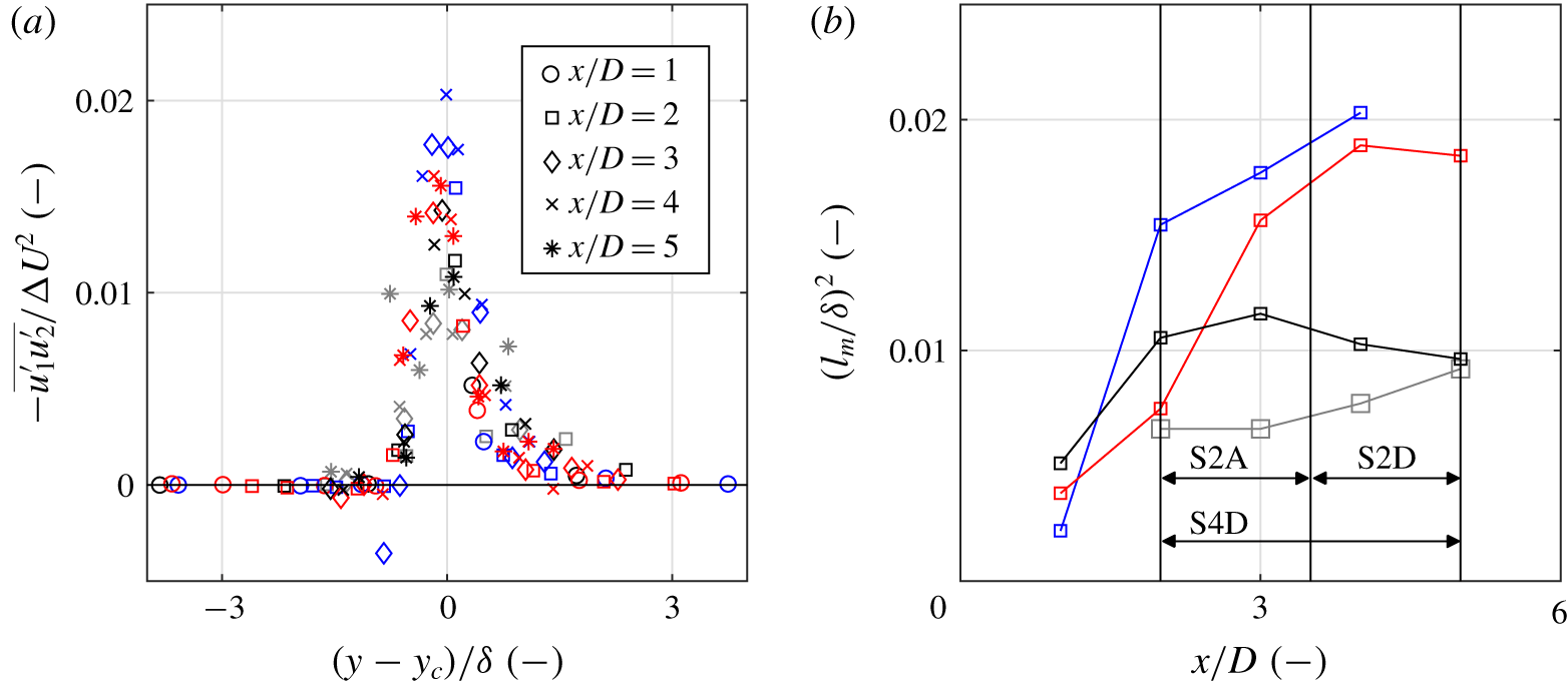
In figure 9 the measured lateral profiles of the streamwise velocity are collected. The profile (4.1) fits the data quite well, and the mean relative error of the fit is for all cases less than 5 %. Most of the data collapse onto a single hyperbolic tangent (black line), although some scatter remains, mostly on the high-velocity side. This is partly attributed to disturbances of the boundary layer due to the acceleration at the horizontal obstruction, and partly to small inaccuracies in the measurements. The collapse of the streamwise velocities on a single curve supports self-similarity of the horizontal mixing layers.
Lateral profiles of the measured mean depth-averaged streamwise velocities for cases PB (black markers), S2A (blue markers), S4A (red markers) and S2D (grey markers). The lateral  $y$-coordinate is centred on the centreline position $y_{c}$ and scaled with the mixing layer width $\unicode[STIX]{x1D6FF}$. Velocity $U$ is scaled with the velocity difference between the high-velocity ( $U_{hi}$) and the low-velocity ( $U_{lo}$) sides of the mixing layer.

Figure 10 shows lateral profiles of the streamwise velocity component, including the fitted hyperbolic–tangent profile, at several streamwise positions in the domain. The velocity profiles of the mixing layers of cases S2A and S4A (flow attachment) start to differ considerably from the plane bed reference case (PB, black) once they reach the slope. The main flow velocity decreases slightly, but less than would be the case if there were no lateral redistribution, for which velocities would decrease proportionally to the increase in flow depth. For case S2D, the velocity profile at the slope also deviates from the plane bed mixing layer. At the start of the slope these differences are small, but they become larger towards the toe of the slope. Downstream of the slope ( $x/D>5$) the mixing layer structure of the horizontal flow field has almost disappeared. This deviation from the plane bed mixing layer is attributed to a higher energy dissipation at the interface between the mixing layer and the vertical recirculation zone, in a way analogous to the higher energy dissipation by bed friction for a rougher plane bed. Downstream of the slope ( $x/D>5$) this explanation is no longer valid due to vertical mixing of streamwise momentum from the main flow.
Mixing layer profiles as a function of streamwise distance. (a) Lateral profiles of the mean depth-averaged streamwise velocity as a function of the streamwise position  $x/D$. Both fitted (solid lines) and observed (round markers) profiles are plotted for cases PB (black), S2A (blue), S4A (red) and S2D (grey). The extent of the slopes for cases S2A, S2D and S4A are indicated by the arrows above panel (a). (b) Mean depth-averaged lateral profiles of the streamwise velocity at the slope as a function of $x/L_{s}$ for cases S2A (slope 1 in 2, attached; blue) and S4A (slope 1 in 4, attached; red). The start of the slope is at $x/L_{s}=0$ and the toe of the slope at $x/L_{s}=1$.
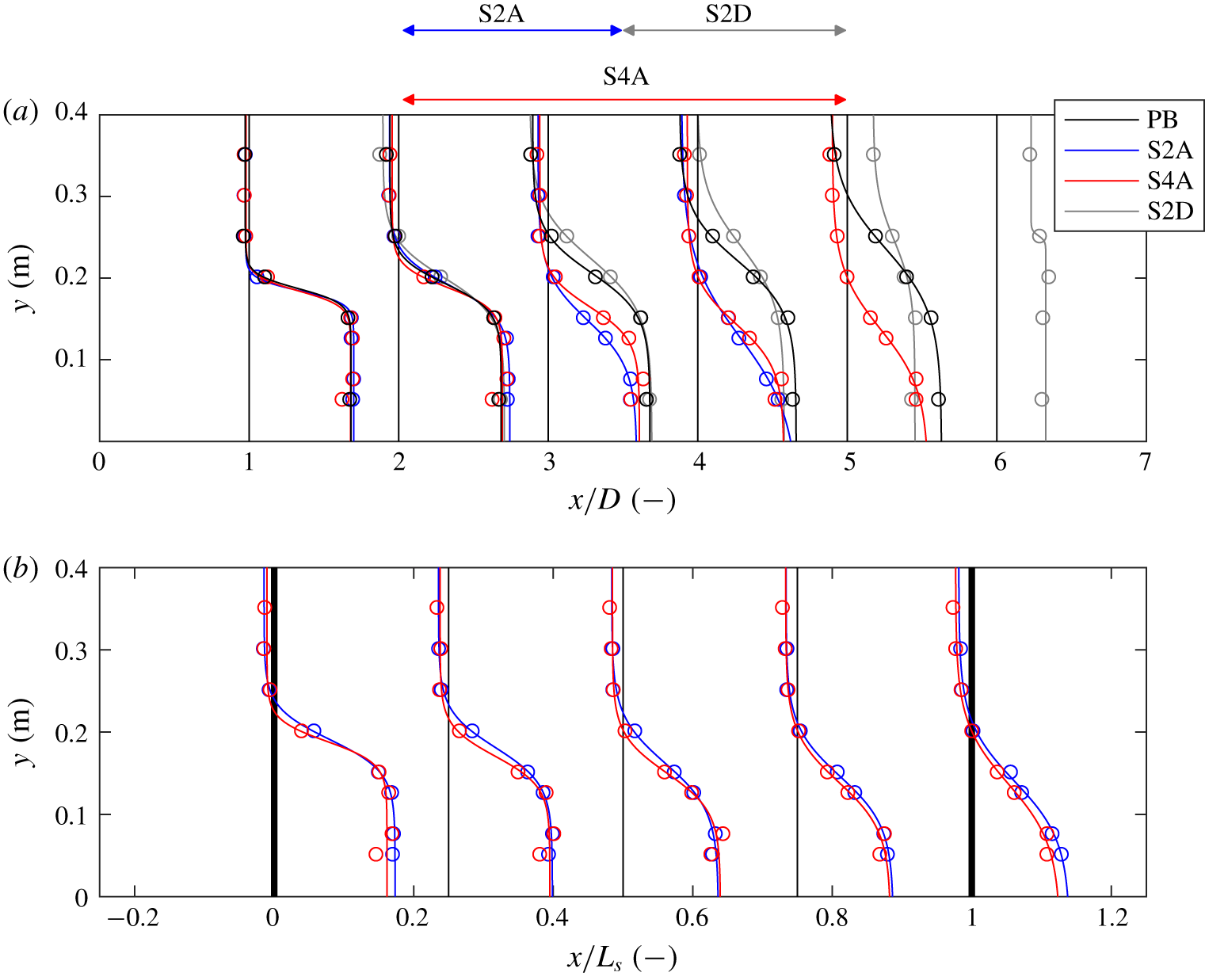
Figure 10(b) shows the velocity profiles of cases S2A and S4A at the slope scaled with the slope length  $L_{s}$. These profiles are largely overlapping, which supports the view that the relative increase in flow depth is a key parameter in shaping the flow field at the slope. In the following, we explain this dependency by considering the different length scales of the problem, supported by the change in mixing layer characteristics $\unicode[STIX]{x0394}U$, $U_{c}$, $\unicode[STIX]{x1D6FF}$ and $y_{c}$, shown in figure 11.
(a) Velocity difference between the high- and low-velocity branches of the mixing layer; (b) lateral position of the mixing layer centreline; (c) velocity at the centreline position of the mixing layer; (d) width of the mixing layer, the bold dash-dotted lines denotes theoretical growth of the mixing layer using (4.2) with  $\unicode[STIX]{x1D6FC}=0.09$ (see Uijttewaal & Booij Reference Uijttewaal and Booij2000). The solid black lines indicate the respective positions of the slope for the sloping cases.
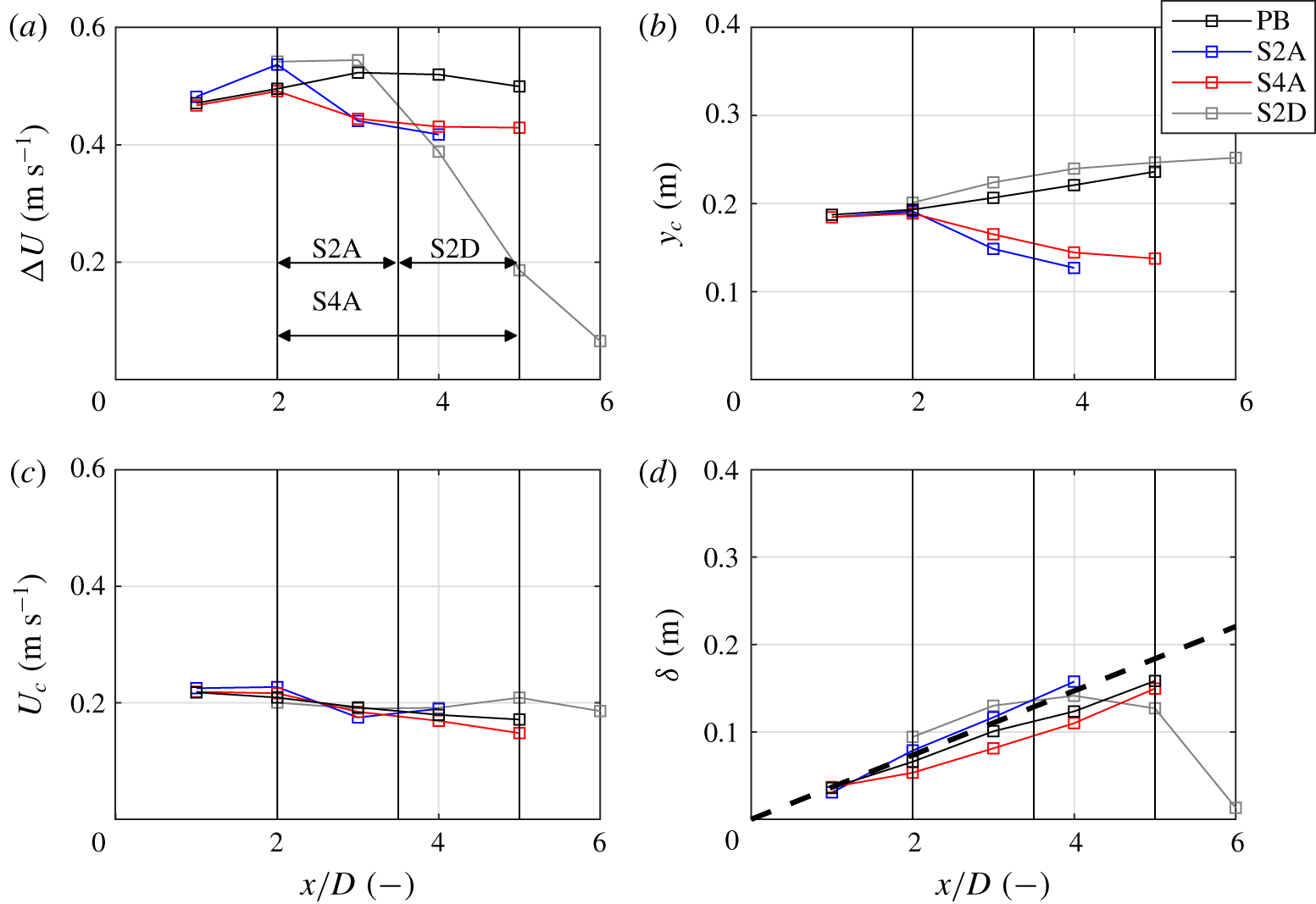
For a plane bed mixing layer, the development of the velocity difference is a function of the bed friction, which causes a deceleration of the high-velocity stream and an acceleration of the low-velocity stream (Uijttewaal & Booij Reference Uijttewaal and Booij2000). As was mentioned before, the friction length scale  $L_{f}$ is much larger than both the expansion width and the slope length. Therefore, in the domain we are considering ( $0<x/D<6$), the effect of bed friction is relatively small. Indeed, figure 11(a) shows that the respective velocity differences are approximately uniform over the domain, with the exception of case S2D. Initially, the velocity difference slightly increases because of the development of the horizontal recirculation zone. For the attached sloping cases, the velocity difference decreases over the distance of the slope. For cases S2A and S4A, the conveyance cross-section of the high-velocity side must become narrower for increasing flow depth, in order to satisfy mass conservation while the velocity difference remains constant. This is visible as a displacement of the mixing layer centre ( $y_{c}$) towards the high-velocity side (figure 11b). This displacement is proportional to the increase in flow depth, explaining the scalability of the horizontal flow field with the length scale of the sloping section, $L_{s}$. This length scale is much shorter than the friction length scale, and this effect dominates the development of the flow field at the slope. A lateral pressure gradient is needed to shift the centre position of the mixing layer, as will be confirmed in § 4.3. For case S2D, $y_{c}$ evolves in the same way as for case PB. At the upstream edge of the slope, $y_{c}$ is larger than for cases S2A and S4A since the mixing layer develops over a longer streamwise distance before it reaches the slope. Given the reduction in velocity difference a larger change in $y_{c}$ might be expected, which indicates that a large part of the reduction in velocity difference is due to vertical mixing of streamwise momentum in the high-velocity stream.
Depth-averaged turbulent kinetic energy. (a) Lateral profiles of the streamwise turbulent kinetic energy  $\overline{u_{1}^{\prime }u_{1}^{\prime }}$, scaled with the velocity difference $\unicode[STIX]{x0394}U^{2}$; (b) lateral profiles of the spanwise turbulent kinetic energy $\overline{u_{2}^{\prime }u_{2}^{\prime }}$, scaled with the velocity difference $\unicode[STIX]{x0394}U^{2}$; for cases PB (black), S2A (blue), S4A (red) and S2D (grey). For case S2D the mixing layer structure of the flow has disappeared after $x/D\approx 5$, so turbulence properties are shown up until this position.

Like the velocity difference, the velocity at the centreline position of the mixing layer is approximately constant over the streamwise distance (figure 11c), such that we can expect the respective mixing layers to grow with a uniform rate. Figure 11(d) shows that, for  $0<x/D<5$, this is indeed the case, with the exception of case S2D. Under the assumption of self-similarity, growth of the mixing layer width is proportional to the relative velocity difference (see van Prooijen & Uijttewaal Reference van Prooijen and Uijttewaal2002),
 $$\begin{eqnarray}\frac{\text{d}\unicode[STIX]{x1D6FF}}{\text{d}x}=\unicode[STIX]{x1D6FC}\frac{\unicode[STIX]{x0394}U}{U_{c}}.\end{eqnarray}$$
 The growth of the respective mixing layers correspond to that of a deep water mixing layer, which is indicated in figure 11(d), using  $\unicode[STIX]{x1D6FC}=0.09$ as reported in Uijttewaal & Booij (Reference Uijttewaal and Booij2000). Figure 11(d) shows that the mixing layer growth is not significantly influenced by the presence of the slope. For case S2D, after $x/D\approx 4$, the mixing layer width declines, which is related both to influence of the sidewall of the flume and to the fact that the mixing layer structure has more or less disappeared from $x/D>5$ onwards (figure 10). To eliminate the influence of the sidewall on mixing layer development, and to further assess the relative importance of bed friction, further experiments can be considered in a wider, shallower flume.
4.2.2 Turbulence properties
Transverse profiles of the mean streamwise and spanwise turbulent kinetic energy (TKE) in the mixing layer are shown in figure 12. For all cases and positions, streamwise TKE is roughly a factor of 2 higher than the spanwise TKE. Generally, both streamwise and spanwise TKE increase with streamwise distance, which indicates that not all turbulence is generated locally but rather that (part of) it is advected from upstream. It is conjectured that, for positions further downstream, where the lateral gradient in streamwise velocity is smaller, turbulence intensities in the centre of the mixing layer will reduce. For the attached sloping cases, S2A and S4A, turbulence intensities at the slope ( $x/D>2$) are larger than for cases PB and S2D. The presence of the slope intensifies turbulence, an effect that is also recognized in the lateral profiles of the horizontal Reynolds shear stress (figure 13a), which, for cases S2A and S4A, are higher at the slope. Similarly to the TKE, the Reynolds stress increases with the streamwise distance. The horizontal Reynolds stress is of the same order of magnitude as the turbulent kinetic energy, which indicates a significant exchange of momentum over the mixing layer. This exchange is highest for case S2A (blue markers), indicating that the steepness of the slope plays an important role in lateral momentum exchange.
Depth-averaged lateral turbulence characteristics. (a) Lateral profiles of the horizontal component of the Reynolds stress,  $\overline{\unicode[STIX]{x1D70F}}_{xy}=-\overline{u_{1}^{\prime }u_{2}^{\prime }}$, scaled with the velocity difference $\unicode[STIX]{x0394}U^{2}$; (b) Ratio between mixing length and mixing layer width, $(l_{m}/\unicode[STIX]{x1D6FF})^{2}$ as a function of streamwise distance; for cases PB (black), S2A (blue), S4A (red) and S2D (grey). For case S2D the mixing layer structure of the flow has disappeared after $x/D\approx 5$, so turbulence properties are shown up until this position.
The intensification of the turbulence due to the slope may influence the mixing length ( $l_{m}$), which can be estimated from the Reynolds stress, $\overline{u_{1}^{\prime }u_{2}^{\prime }}$, as follows (see Uijttewaal & Booij Reference Uijttewaal and Booij2000):
 $$\begin{eqnarray}\left(\frac{l_{m}}{\unicode[STIX]{x1D6FF}}\right)^{2}=\frac{-\overline{u_{1}^{\prime }u_{2}^{\prime }}|_{max}}{\unicode[STIX]{x0394}U^{2}}.\end{eqnarray}$$
 The right-hand side of (4.3) is plotted in figure 13(a) for several streamwise positions. For cases PB and S2D  $\left(l_{m}/\unicode[STIX]{x1D6FF}\right)^{2}$ has the order of 0.01, which is the same as the value found by Uijttewaal & Booij (Reference Uijttewaal and Booij2000) for plane bed mixing layers. For cases S2A and S4A $(l_{m}/\unicode[STIX]{x1D6FF})^{2}$ is approximately twice as large. As can be seen in figure 13(b), the mixing length is largest for case S2A, which implies that the steepness of the slope is an important parameter for horizontal mixing. The influence of the slope on the development of large turbulent structures is evident, and the role of these structures in the lateral exchange of momentum will therefore be the topic of future studies.
The dynamics of a mixing layer over a streamwise sloping bed is self-similar. In the case of vertical flow separation, in the near-field area that we have studied, the behaviour of the mixing layer in the upper part of the water column is very similar to that of a plane bed mixing layer. The differences between the cases are interpreted as the result of additional energy dissipation at the interface of the main flow and the vertical recirculation zone, analogously to higher energy dissipation due to a rougher bed. In the case of vertical flow attachment, a strong dependency of the shape of the horizontal flow field on the increase in depth was found, which was explained through mass conservation. The flow redistributes such that the conveyance cross-section elongates in the vertical direction and compresses in the horizontal direction.
Analysis of the horizontal mixing layer dynamics provided insight into the differences in flow conditions between the selected cases. However, analysis of the horizontal flow fields does not reveal why the flow stays attached to the bed in some cases, whereas it separates from the bed in others. Since boundary layer development is, in general terms, driven by a balance between bed shear stress and pressure gradients, the next section will consider the pressure fields of cases S2A (slope 1 in 2, attached) and S2D (slope 1 in 2, separation) to identify possible differences between an attached and a separating case.
4.3 Piezometric head and total energy head
Boundary layer separation at the sloping bed is largely governed by the pressure gradient in the main flow over the slope. The present experimental set-up did not measure these gradients directly; however, the corresponding pressure fields can be reconstructed from the respective momentum balances. In this section, first the methodology to reconstruct the pressure field is discussed. Next, results of this operation are presented and discussed. Finally, using the reconstructed pressure field the mean total energy head is derived and presented.
4.3.1 Pressure field reconstruction
First, a brief description is provided regarding the methodology used to derive the pressure field from the observed velocity measurements, using the respective momentum balances. To this end, consider the stationary Reynolds-averaged Navier–Stokes equations
 $$\begin{eqnarray}\frac{\unicode[STIX]{x2202}\overline{u}_{i}\overline{u}_{j}}{\unicode[STIX]{x2202}x_{j}}+\frac{\unicode[STIX]{x2202}\overline{u_{i}^{\prime }u_{j}^{\prime }}}{\unicode[STIX]{x2202}x_{j}}+\frac{\unicode[STIX]{x2202}\overline{P}/\unicode[STIX]{x1D70C}}{\unicode[STIX]{x2202}x_{i}}-\frac{\unicode[STIX]{x2202}}{\unicode[STIX]{x2202}x_{j}}\unicode[STIX]{x1D708}\left(\frac{\unicode[STIX]{x2202}\overline{u}_{i}}{\unicode[STIX]{x2202}x_{j}}+\frac{\unicode[STIX]{x2202}\overline{u}_{j}}{\unicode[STIX]{x2202}x_{i}}\right)=\overline{f}_{i},\end{eqnarray}$$
 where  $i,j=1,2,3$; $\overline{P}$ is the mean pressure ( $\text{kg}~\text{ms}^{-2}$) in excess of the constant atmospheric pressure; $\unicode[STIX]{x1D70C}$ is a constant density (fresh water, $1000~\text{kg}~\text{m}^{-3}$); $\unicode[STIX]{x1D708}$ is the kinematic molecular viscosity ( $10^{-6}~\text{m}^{2}~\text{s}^{-1}$); and $\overline{f}$ is the mean body force per unit mass accounting for gravity ( $g=9.81~\text{m}~\text{s}^{-2}$). For convenience, the gravity body force is eliminated by incorporating it in the pressure gradient. This introduces the so-called piezometric head defined by $\overline{h}=z+\overline{P}/\unicode[STIX]{x1D70C}g$. Physically, $\overline{h}$ is the height to which the mean pressure will raise a column of fluid. Eliminating $\overline{P}$ and $\overline{f}$ in favour of $\overline{h}$ and neglecting the viscous terms, which is allowed for the high Reynolds numbers involved, equation (4.4) reduces to
 $$\begin{eqnarray}\frac{\unicode[STIX]{x2202}\overline{u}_{i}\overline{u}_{j}}{\unicode[STIX]{x2202}x_{j}}+\frac{\unicode[STIX]{x2202}\overline{u_{i}^{\prime }u_{j}^{\prime }}}{\unicode[STIX]{x2202}x_{j}}+g\frac{\unicode[STIX]{x2202}\overline{h}}{\unicode[STIX]{x2202}x_{i}}=0.\end{eqnarray}$$
 The first two terms of (4.5), i.e. the divergence of the mean momentum flux, can be estimated from the measurements, which leaves the piezometric level as an unknown field. To compute it in a systematic way, a mesh consisting of tetrahedrons is constructed with the velocity measurement locations as nodal points. On this mesh, a basis of linear interpolation functions is defined to approximate the piezometric level by a, yet unknown, interpolated field  $\overline{h}_{I}$. The best approximation to $\overline{h}_{I}$ is now obtained by minimizing, in a least squares sense, the residual of (4.5),
 $$\begin{eqnarray}\min _{\overline{h}_{I}}\;\int _{V}\frac{1}{2}\left\Vert \frac{\unicode[STIX]{x2202}\overline{u}_{i}\overline{u}_{j}}{\unicode[STIX]{x2202}x_{j}}+\frac{\unicode[STIX]{x2202}\overline{u_{i}^{\prime }u_{j}^{\prime }}}{\unicode[STIX]{x2202}x_{j}}+g\frac{\unicode[STIX]{x2202}\overline{h}_{I}}{\unicode[STIX]{x2202}x_{i}}\right\Vert ^{2}\text{d}V,\end{eqnarray}$$
 where  $V$ denotes the fluid volume captured by the mesh, and $\Vert \cdot \Vert$ denotes a (quadratic) $L^{2}$-norm. Carrying out the minimization with respect to $\overline{h}_{I}$ leads to a Poisson equation,
 $$\begin{eqnarray}\frac{\unicode[STIX]{x2202}^{2}\overline{h}_{I}}{\unicode[STIX]{x2202}x_{i}\unicode[STIX]{x2202}x_{i}}=-\frac{1}{g}\frac{\unicode[STIX]{x2202}}{\unicode[STIX]{x2202}x_{i}}\left(\frac{\unicode[STIX]{x2202}\overline{u}_{i}\overline{u}_{j}}{\unicode[STIX]{x2202}x_{j}}+\frac{\unicode[STIX]{x2202}\overline{u_{i}^{\prime }u_{j}^{\prime }}}{\unicode[STIX]{x2202}x_{j}}\right).\end{eqnarray}$$
 The right-hand side of (4.7) is computed directly from the measured velocity field after which the solution for  $\overline{h}_{I}$ is obtained using the standard finite element method (e.g. Labeur Reference Labeur2009). We will refer to the computed piezometric level as $\overline{h}$, omitting the subscript $I$ for brevity.
The piezometric head is determined with the same accuracy as the observed stress tensor, up to an unknown constant. Since our main interest is the gradient of  $\overline{h}$, this constant can be chosen arbitrarily. We therefore set $\overline{h}$ equal to zero at the surface in a transect in the high-velocity stream of the mixing layer, at the upstream edge of the slope. This position is indicated in figure 14 using a black cross.
Mean piezometric head for cases S2A (a,c,e) and S2D (b,d,f). (a,b) Horizontal  $xy$ plane near the free surface. Black lines indicate the location of the slope, the red lines the location of the vertical $xz$ cross-section; (c,d) vertical $xz$ plane in the high-velocity stream of the mixing layer; (e,f) vertical $xz$ plane in the low-velocity stream of the mixing layer. The streamwise coordinate is scaled with the width of the expansion $D$, vertical coordinate is scaled with the upstream depth $d_{u}$. The blue line in panels (c–f) is the free-surface level at the inflow boundary, that is, $d_{u}=0.12~\text{m}$. The black cross denotes the location of the (arbitrary) reference level $\overline{h}=0$.

4.3.2 Piezometric head
Figure 14 shows the constructed fields of the piezometric head for cases S2A and S2D. For a straightforward comparison of these cases the upstream edge of the respective slopes is taken as the origin  $x/D=0$. For case S2A, $\overline{h}$ increases with almost 2 mm over the slope, while for case S2D a decrease of almost 2 mm is observed. This is attributed to differences in pressure recovery between an attached and a separated flow, respectively, which is discussed below. For both cases, the corresponding gradient of $\overline{h}$, which is also a measure of the free-surface slope, is of the order of $O(10^{-3})$. As a comparison, the free-surface slope caused by friction (i.e. the friction slope: $i_{f}=-c_{f}U^{2}/gd$) is of the order of $O(10^{-4})$ – as can be inferred from a one-dimensional depth-averaged momentum equation. In the region of the sloping bed, free-surface effects are therefore dominated by advective momentum transport gradients, rather than bed friction, which plays a secondary role here.
Figure 14(a,b) shows a slight variation of the piezometric head in the transverse direction for both case S2A and case S2D. The near uniformity of  $\overline{h}$ in the transverse direction is consistent with the small horizontal curvature of the observed streamlines, which supports the validity of the computed pressure fields. Figure 14(c–f) shows the variation of the piezometric head in the vertical direction. For both case S2A and case S2D this variation is larger on the high-velocity side of the mixing layer than it is on the low-velocity side, where the vertical pressure distribution is almost hydrostatic (the piezometric head is vertically uniform).
Figure 15 shows the spatial variation of  $\overline{h}$ in more detail for the high- and low-velocity sides of the mixing layers – near the bed as well as near the surface – along horizontal lines indicated in red in figure 14. Starting from the upstream edge of the slope, $\overline{h}$ increases with streamwise distance for case S2A while it decreases for case S2D, which once more illustrates the difference in development of $\overline{h}$ between these cases.
Using figures 14 and 15, we now analyse the variation of the piezometric level over the vertical in more detail. For case S2A,  $\overline{h}$ is slightly higher near the bed than near the surface, despite the curvature of the streamlines at the upstream edge of the slope. This feature is explained by considering that, besides the curvature, the streamlines are vertically diverging in the vicinity of the slope due to the increase in flow depth. The curvature that results from the increase in flow depth is dominant with respect to the curvature of the streamlines over the edge of the slope.
Vertical variability is largest upstream of the slope in the high-velocity stream of the mixing layer. Near the bed  $\overline{h}$ is higher than near the surface for both cases. Values of $\overline{h}$ decrease towards the upstream edge of the slope. For case S2A, this decrease is largest. Near the surface, $\overline{h}$ increases with streamwise distance for case S2D whilst it is more or less constant for case S2A. These observations motivate a further analysis of the boundary layer dynamics in the vicinity of the slope to understand the differences between a vertically attaching case and a separating case.
The variation of  $\overline{h}$ in the transverse direction is considered here using figure 15. The observed changes in centreline position (figure 11) and attributed curvature of the streamlines as observed in the depth-averaged flow fields (figure 6) involve a lateral pressure gradient. Derived values of $\overline{h}$ confirm this for both cases S2A and S2D. For case S2A, $\overline{h}$ is higher on the low-velocity side than the high-velocity side for $-0.5<x/D<2$, which is the sloping region; outside of the sloping region, transverse variation of $\overline{h}$ is reversed. For case S2D, $\overline{h}$ is higher on the high-velocity side than on the low-velocity side. The rate of change of $\overline{h}$ is highly similar for both branches of the mixing layer for both cases.
Streamwise profiles of the piezometric head along the flume for cases S2A (blue and grey-blue) and S2D (grey and dark-red) The location of the streamwise profiles are indicated in figure 14. Piezometric head is plotted on the high-velocity side (solid lines) and the low-velocity side (dashed lines) near the free surface (blue and grey) and near the bed (grey-blue and dark-red). The abbreviations in the legend stand for high-velocity side, surface (HS); high-velocity side, bed (HB); low-velocity side, surface (LS); low-velocity side, bed (LB). The reference level was chosen such that HS for both cases starts at  $\overline{h}=0$. The black dotted line is the friction slope $i_{f}$ inferred from a one-dimensional depth-averaged momentum equation.
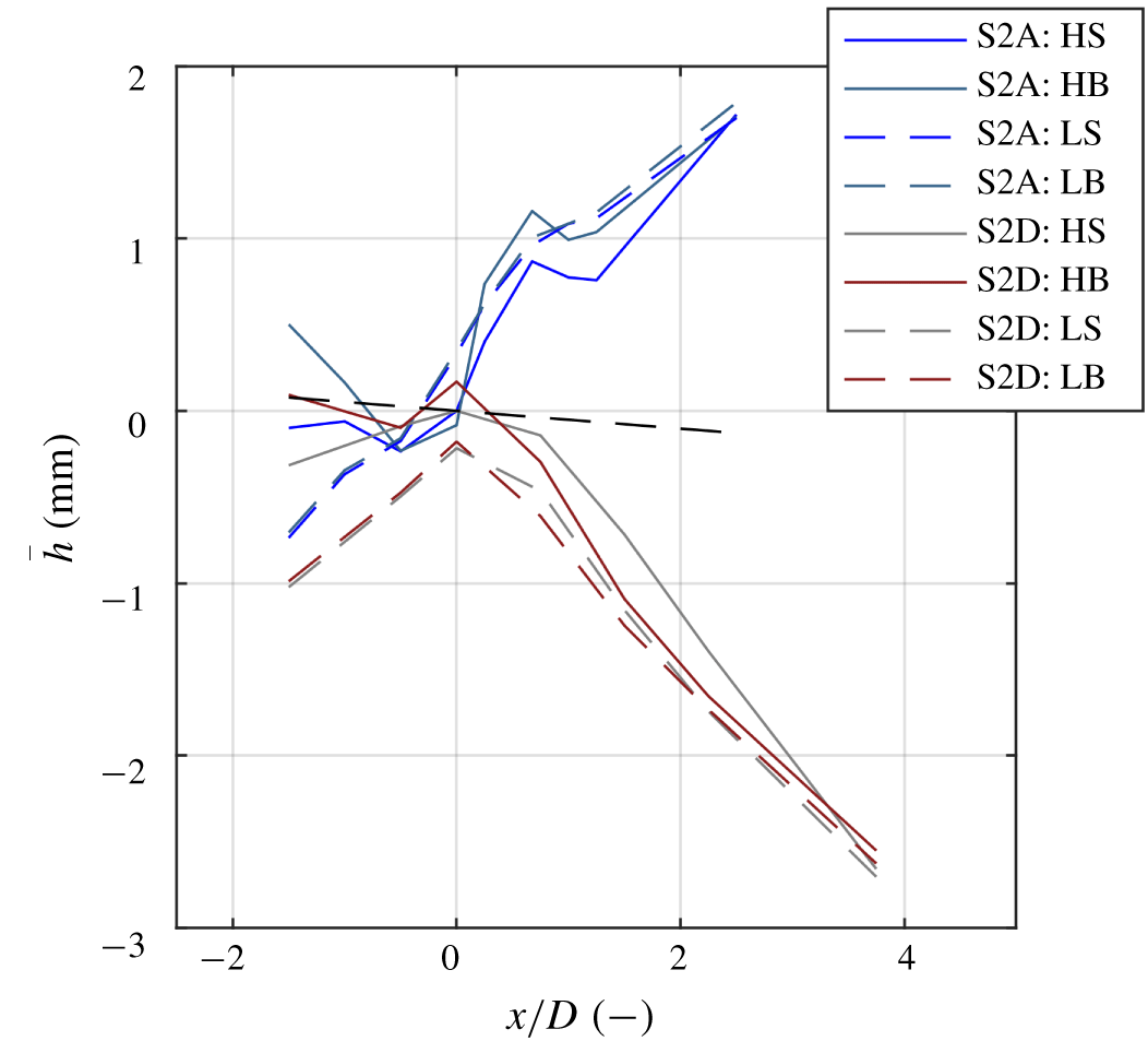
Mean total energy head  $\overline{H}=\overline{h}+{\textstyle \frac{1}{2}}\overline{u_{i}u_{i}}/g$ for cases S2A (a,c,e) and S2D (b,d,f). (a,b) Horizontal $xy$ plane near the free surface. Black lines indicate the location of the slope, the red lines the location of the vertical $xz$ cross-section; (c,d) vertical $xz$ plane on the high-velocity side of the mixing layer; (e,f) vertical $xz$ plane on the low-velocity side of the mixing layer. Streamwise coordinate is scaled with the width of the expansion $D$, vertical coordinate is scaled with the upstream depth $d_{u}$. The blue line in panels (c,f) is the free-surface level at the inflow boundary, that is, $d_{u}=0.12~\text{m}$. The reference level for $h$ is chosen such that $h$ is zero at the start of the slope on the high-velocity stream.

4.3.3 Mean total energy head
The mean total energy head, defined by  $\overline{H}=\overline{h}+{\textstyle \frac{1}{2}}\overline{u_{i}u_{i}}/g$, is obtained from the reconstructed piezometric head and the observed mean kinetic energy. As for the piezometric level, this quantity can be determined up to a constant so that only the changes in $\overline{H}$ can be considered. For consistency, the same reference level as used for the piezometric level $\overline{h}$ is adopted. Figure 16 shows the mean total energy head for case S2A and case S2D using the same horizontal and vertical transects as used in figure 14 for the piezometric head.
Along the high-velocity side of the mixing layer (figure 16a,b) the rate of change of  $\overline{H}$ is comparable for both cases, while downstream of the bed slope $\overline{H}$ rapidly decreases for case S2D and slightly decreases for case S2A. Hence, case S2A is less dissipative than case S2D. This explains the pressure recovery over the slope for case S2A that is largely absent for case S2D.
For case S2A, the high-velocity side of the mixing layer shows little variation of  $\overline{H}$ over the depth (figure 16c), which further supports vertical uniformity of this case. For case S2D, the high-velocity side shows significant variation of $\overline{H}$ over the depth (figure 16d). This involves vertical mixing of streamwise momentum causing a decrease, in the streamwise direction, of $\overline{H}$ in the upper water column. The vertical mixing also contributes to the observed reduction of the velocity difference over the horizontal mixing layer for case S2D (figure 11a,b).
Along the low-velocity side (figure 16e,f) both cases show an increase of  $\overline{H}$ in the streamwise direction which is due to lateral exchange of momentum across the mixing layer. This also results in an increasing magnitude of the return current in the horizontal recirculation zone.
The computed pressures and energy head levels are consistent with the outcome of the previous analyses. However, they do not fully explain the observed suppression of flow separation for steeper lateral gradients of the streamwise velocity.
5 Discussion
5.1 Vertical flow separation or attachment?
In Broekema et al. (Reference Broekema, Labeur and Uijttewaal2018) a possible explanation for the suppression of vertical flow separation due to lateral non-uniformity was given, based on the horizontal convergence of the flow over a sloping section. Due to the horizontal convergence, the adverse pressure gradient reduces, and vertical flow separation does not occur. For milder slopes, this horizontal convergence of the flow has been observed in several experiments (MacVicar & Rennie Reference MacVicar and Rennie2012; MacVicar & Best Reference MacVicar and Best2013; Chartrand et al. Reference Chartrand, Mark Jellinek, Hassan and Ferrer-Boix2018) and in field situations (MacVicar & Roy Reference MacVicar and Roy2007). For steeper slopes, like the field observations of Broekema et al. (Reference Broekema, Labeur and Uijttewaal2018) and the current experiment, the horizontal flow pattern relates to the suppression or occurrence of vertical flow separation. For shallow environmental flows, the mutual interaction between the horizontal and vertical flow state was explained by Broekema et al. (Reference Broekema, Labeur and Uijttewaal2018) to be the result of conservation of potential vorticity; if the convergence of the flow due to potential vorticity conservation is sufficiently large, the adverse pressure gradient is reduced and flow separation is suppressed.
In horizontal shear flows like jets, mixing layers and wakes, vorticity in the shear layer is predominantly made up of the lateral gradient in streamwise velocity,  $\unicode[STIX]{x2202}U/\unicode[STIX]{x2202}y\approx \unicode[STIX]{x0394}U/\unicode[STIX]{x1D6FF}$. The transition from a vertically attached and horizontally converging flow state towards a vertically separating and horizontally diverging flow state occurred for milder lateral gradients in streamwise velocity. This is in line with the reasoning of Broekema et al. (Reference Broekema, Labeur and Uijttewaal2018). Although the analogy between the vertical stretching and horizontal compression of the conveyance cross-section with the vertical stretching of a single vortex is still recognized in the observed flow field (§ 4.1), it was shown in § 4.2 that for the selected cases there are no significant differences in the development of the velocity difference over the mixing layer ( $\unicode[STIX]{x0394}U$) and the mixing layer width ( $\unicode[STIX]{x1D6FF}$). Therefore, the phenomena observed during this study cannot be exclusively related to potential vorticity conservation.
Because of the enhanced energy dissipation and the resulting lowering of the piezometric head for the vertically separating case we cannot directly relate the adverse pressure gradient to the transition between flow states. Although the pressure varies over the width and depth of the flume, the streamwise pressure gradient throughout the domain is highly uniform. Based on this observation, we hypothesize that there is a difference between the global and the local behaviour of the flow. The overall pressure gradient is linked to the bulk motion of the fluid, while it has a different impact on the high- and low-velocity streams. The data do not conclusively prove or disprove this hypothesis, and further analysis is required.
Another possible explanation for the transition between the two possible flow states may originate from the unstable nature of the flow around the transition point. Analysis of the flow fields showed that one of the key parameters in controlling the occurrence of vertical flow separation is the steepness of the lateral gradient of the streamwise velocity at the upstream edge of the slope. Steeper gradients generally give rise to higher locally generated turbulence intensity and instabilities. It was shown that the slope intensified the turbulence, which could potentially induce a larger lateral exchange of momentum. As a result, the horizontal recirculation zone grows larger, and through its growth, compresses the high-velocity branch of the mixing layer, implying that the vertical flow state is coupled to the occurrence of a horizontal recirculation zone. The transition between one flow state and the other is then the result of a global instability of the flow that is possibly triggered by the combination of steep lateral gradients and a disturbance in the bed topography. The flow development phase was not studied in a detailed manner during the course of this work. However, high-resolution numerical modelling of the phenomena may further reveal these intricacies.
5.2 Application
We now briefly consider the case that inspired this experimental study; the large-scale local erosion that is observed downstream of a storm surge barrier in the Netherlands (Broekema et al. Reference Broekema, Labeur and Uijttewaal2018). Field observations have shown the occurrence of large lateral gradients in the streamwise velocity, in combination with a strong horizontal convergence towards the deepest point of the erosion in combination with an absence of vertical flow separation. It was shown in § 3.3 that whether or not the flow stays attached makes a great difference for the occurring bed shear stress. This is a secondary effect; while the bed shear stress is, compared to the other terms in the momentum equation, relatively small, it is the primary cause of the erosion. As a result, the erosion may continue and lead to an even stronger horizontal convergence. Furthermore, the streamwise increase in depth was shown to amplify the turbulence intensity. Thus, a positive feedback mechanism is revealed, where the combination of the eroded topography and a laterally non-uniform flow may sustain or even increase ongoing erosion. These phenomena may play a large role in comparable situations as well, since in confined geophysical and technical flows lateral non-uniformity is the rule rather than the exception.
Another possible application of the present results concerns flow control. Although this was not the primary aim of this study, the fact that horizontal convergence of the flow at a deepening can suppress vertical flow separation may serve as an inspiration for new flow control strategies. Inducing flow separation in the horizontal  $xy$ plane to suppress flow separation in the vertical seems counterintuitive. However, one may for instance think of a deflection screen that gradually contracts the flow horizontally. Guiding the flow through such a constriction before it enters a region of vertical expansion (a deepening) may limit energy losses that would otherwise have occurred.
6 Conclusions
Separation of flow and flow control methods have been the subject of decades of research, and this study provides additional insight into the drivers of these phenomena. This work demonstrates – for the first time – that vertical flow separation can be suppressed by horizontally contracting a flow, even for steep slopes of up to 1 in 2 ( $\pm 26^{\circ }$). These findings inspire further experimental and numerical studies into both the three-dimensional character of the phenomena as well as their broader implications.
Two clearly distinct flow states were defined and characterized in this study; (i) a combination of vertical flow attachment and horizontal convergence, and (ii) a combination of vertical flow separation and horizontal divergence. The character of the flow is inherently three-dimensional, but the horizontal flow field is well described by a depth-averaged framework in case the flow stays vertically attached. The conveyance cross-section is elongated vertically in this case, and compressed in the horizontal plane. The horizontal convergence of the flow at the slope is then a function of the increase in flow depth. In case of vertical flow separation, the conveyance cross-section of the flow is mainly confined to the upper part of the water column. Horizontal mixing layer development in the conveyance cross-section is analogous to the development of a plane bed mixing layer, with added energy dissipation originating from the shear between the main flow and the vertical recirculation zone. The combination of horizontal convergence and vertical attachment of the flow was shown to lead to considerably higher bed shear stresses compared to a separating flow, as well as to an amplification of horizontal turbulence intensities.
The convergence in the horizontal plane can explain the suppression of flow separation in the vertical plane, although pressure fields computed from the obtained velocity data do not decisively confirm this hypothesis. The present observations provide new insight into the dynamics, and consequences, of three-dimensional flow separation, but the parameter space is still too limited to conclusively determine the transition point between the observed flow states. To this end, additional high-resolution experimental or numerical data and analyses are required. These may provide further insight into, amongst others, the pressure distribution, the structure of the boundary layer, the role of bed friction and the initial configuration of the flow field prior to the transition.
Acknowledgements
The Dutch Ministry of Public Works, Rijkswaterstaat, is gratefully acknowledged for funding this research. All data used in this study will be publicly available on https://data.4tu.nl/, and should be cited as Broekema (Reference Broekema2019). Please see the reference list for full reference details.
Declaration of interests
The authors report no conflict of interests.
Supplementary movie
Supplementary movie is available at https://doi.org/10.1017/jfm.2019.972.


 Open access