


When did spouses start matching closely on their socioeconomic characteristics? This question is important because, in recent decades, developed economies have seen an increase in both female labor force participation rates and educational attainment (Goldin Reference Goldin2006; Piketty and Saez Reference Piketty and Saez2014). This has led to widespread concern that marriage has become more assortative, increasing household inequality. However, empirical evidence from the United States suggests only very modest increases after 1960 (Eika, Mogstad, and Basit Reference Eika, Mogstad and Basit2019; Greenwood et al. Reference Greenwood, Guner, Kocharkov and Santos2014b).Footnote 1 Moreover, this increase in sorting has had little direct impact on household inequality (Greenwood et al. Reference Greenwood, Guner, Kocharkov and Santos2014a; Hryshko, Juhn, and McCue Reference Hryshko, Juhn and McCue2017). Why did the economic empowerment of women seem to matter so little for assortment and inequality?
To explain this puzzle, I argue we must take a longer-run perspective. To examine marriage sorting before female empowerment, it uses an unusually rich dataset from the Canadian Province of Quebec, 1800–1960. This setting is ideal, not only because of the strength of the data but also because of its similarity to other advanced economies and its deeply conservative gender norms.
I find that, despite limited female labor force participation, marriage has always been highly assortative. There was little room for it to become more so. To explain why, this paper adds to the growing literature on historical female mobility by considering the role of maternal human capital on children (Craig et al. Reference Craig, Eriksson, Niemesh and Rashi2023; Olivetti and Paserman Reference Olivetti and Paserman2015). Marriage has always mattered for inequality because mothers have always mattered for child outcomes.
This conclusion is based on the answers to three related empirical questions. First, how did the degree of marital assortment evolve over the long run? Historical studies are often limited due to missing data on married women (Olivetti et al. 2020). In the spirit of Chadwick and Solon (Reference Chadwick and Solon2002), I develop a novel method to overcome this limitation. Using the method, I estimate a correlation between spouses that is surprisingly strong—around 0.85—and stable over time. It has since been extended to other contexts by Clark and Cummins (Reference Clark and Cummins2022), Clark, Cummins, and Curtis (Reference Clark, Cummins and Curtis2022), Luo (Reference Luo2022), and Clark (Reference Clark2023).
Second, was matching merely the result of negotiation between families of similar socioeconomic status (Puga and Trefler Reference Puga and Trefler2014)? Instead, I find evidence that individual human capital mattered. For example, a woman who could sign her name married a man 34 percentage points more likely to sign his name than her sister, who could not.
Third, did mothers influence child outcomes directly? As marriages were assortative, it is challenging to untangle the independent effect of a mother (Espín-Sánchez, Gil-Guirado, and Vickers Reference Espín-Sánchez, Gil-Guirado and Vickers2022). Using the unusually high frequency of remarriage to control for the father, I find evidence that the human capital of mothers had an independent effect on child outcomes (at least for those who married twice). Together, the answers to these questions demonstrate that marriage sorting mattered long before married women held formal employment.
I can answer these questions by using millions of linked marriage records from the BALSAC database (Project BALSAC Reference BALSAC2020).Footnote 2 These data have several unique features that make them particularly suitable to answer these questions. First, Québécoise women retained their family name after marriage and thus can be linked to their parents. Linking married women is much harder in societies such as the United States, where women typically take their husbands’ surnames (Craig et al. Reference Craig, Eriksson, Niemesh and Rashi2023). Second, the data are close to a complete population registry. Families in the sample are not selected by cohabitation (like in census records) or by living descendants (like in most genealogical datasets). The large sample size and complete family linkages allow me to untangle the underlying mechanisms linking sorting and mobility.
This paper thus contributes to the literature on marriage sorting. Economists have long recognized the theoretical link between assortative marriage and inequality. I argue that while assortment might not have substantially increased inequality when female labor force participation rose, it has always increased inequality through social mobility (Eika, Mogstad, and Basit Reference Eika, Mogstad and Basit2019; Greenwood et al. Reference Greenwood, Guner, Kocharkov and Santos2014a; Hryshko, Juhn, and McCue Reference Hryshko, Juhn and McCue2017). Borrowing from the intergenerational mobility literature, I develop a new method to account for attenuation bias in measures of assortment (Modalsli and Vosters Reference Modalsli and Vosters2024; Nybom and Stuhler Reference Nybom and Stuhler2017; Ward Reference Ward2023). By doing so, it relates to other papers on the difficulty of estimating marital assortment (Chiappori, Dias, and Meghir Reference Chiappori, Dias and Meghir2020; Liu and Lu Reference Liu and Lu2006). By discussing how matches were formed, it also adds to the growing literature on the mechanisms of marital assortment, both historical and intergenerational (Abramitzky, Delavande, and Vasconcelos Reference Abramitzky, Delavande and Vasconcelos2011; Fagereng, Guiso, and Pistaferri Reference Fagereng, Guiso and Pistaferri2022; Goñi Reference Goñi2022). Finally, while trends in sorting are well studied after the mid-twentieth century, this paper joins the few studies that extend the analysis further into the past (Bailey and Lin Reference Bailey, Lin, Martha, Leah and William2025; Clark and Cummins Reference Clark and Cummins2022; Craig et al. Reference Craig, Eriksson, Niemesh and Rashi2023; Schwartz and Mare Reference Schwartz and Mare2005; Shiue and Keller Reference Shiue and Keller2022).
This paper also adds to our understanding of historical intergenerational mobility. Studies of intergenerational mobility have often overlooked women (Black and Devereux Reference Black, Devereux, Ashenfelter and Card2011). Recent work has emphasized the need to focus on the mobility of daughters as well as sons (Chadwick and Solon Reference Chadwick and Solon2002). However, there are major data challenges to overcome in historical studies of female mobility. Measures of female socioeconomic status are rarely reported, so studies often rely on husbands’ incomes or occupations as a proxy (Dribe, Eriksson, and Scalone Reference Dribe, Eriksson and Scalone2019). In many societies, linking married daughters to fathers requires either pseudo-linkages on first names or recovering their maiden names from marriage records (Craig et al. Reference Craig, Eriksson, Niemesh and Rashi2023; Goñi Reference Goñi2022; Olivetti and Paserman Reference Olivetti and Paserman2015; Olivetti et al. 2020). As the records from Quebec have both a proxy for female human capital (signatures) and direct female linkages, they are unusually well-suited to considering historical mobility. Moreover, I follow Espín-Sánchez, Gil-Guirado, and Vickers (Reference Espín-Sánchez, Gil-Guirado and Vickers2022) in explicitly considering the role of mothers as well as daughters. In doing so, I add to the growing literature that considers the role of relatives other than fathers in historical mobility (Olivetti, Paserman, and Salisbury 2018).
The structure of the paper is as follows. I start with a discussion of the historical context, arguing that Quebec 1800–1970 is an ideal setting to consider assortative marriage over the long run. Then, I describe the data, highlighting its unique strengths and explaining how I construct measures of human capital. Next, I develop a novel method to estimate the degree of assortment that is particularly suited to historical contexts. Then, I adapt a simple model showing conditions under which assortment can decrease intergenerational mobility. Next, I present three related empirical findings. First, using my new method, I find the degree of assortment to be surprisingly high and stable throughout the period. Second, I show that this assortment consisted of matching between individuals, not families. Third, I estimate the independent effect of maternal human capital on child outcomes. Together with the simple model, these results suggest assortment was decreasing social mobility. I discuss the broader implications of these findings for the historical mobility literature. Finally, I conclude that assortment mattered for inequality long before the mid-twentieth century because women have always played an important role in marriage and mobility.
HISTORICAL CONTEXT
Quebec 1800–1970 was in many ways very similar to the rest of North America. However, as I will discuss, it had relatively conservative gender norms. This makes it a useful setting to consider the role of women in assortative marriage and social mobility.
While its economic development lagged behind other North American regions, Quebec followed the same trends. For example, it had lower wages until the mid-twentieth century, but the gap was stable over time (Albouy Reference Albouy2008; Geloso and Lindert Reference Geloso and Lindert2020). Quebec had lower social mobility than the rest of Canada, but Canada as a whole was more mobile than Europe (Antonie et al. Reference Antonie, Inwood, Minns and Summerfield2022). Before its Quiet Revolution of the 1960s, Quebec was also much less secular than its neighbors.Footnote 3 Catholicism asserted significant control over public education and social norms, and deeply conservative beliefs about gender roles were enshrined by law and public policy. For a population of European descent, the Québécoise experienced a late demographic transition and unusually large family sizes (Vézina, Gauvreau, and Gagnon Reference Vézina, Gauvreau and Gagnon2014). Married women spent much of their adult lives pregnant and raising small children. Altogether, Quebec before the mid-twentieth century is not a promising time or place to find an important role for female human capital in assortative marriage and child outcomes. As I find just that, it is likely that it was also the case in other places with higher levels of female empowerment.
The Legal Rights of Women
Women in most historical societies faced systematic legal disadvantages; Quebec was no exception. While Quebec was ceded to the British in 1763, laws pertaining to civil matters remained governed by the Coutume de Paris, a codified system of customary French law. With some modifications, these customs were incorporated into the 1866 Civil Code of Lower Canada, which was in force until 1994 (McCord Reference McCord1867). Under Quebec law, and unlike in English-speaking legal traditions, married couples formed a legal entity called the communauté de biens (community of property), in which both partners theoretically have equal stakes (Greer 1997). Therefore, both the husband and wife were required to sign legal documents,Footnote 4 though the husband alone was expected to manage the joint property.
After marriage, women were legally considered incapable, being unable to independently form contracts or initiate lawsuits (Baillargeon Reference Baillargeon and Wilson2014). The reformed Civil Code of Lower Canada, introduced in 1866, only clarified the legal disadvantages faced by women. While Québécoise women could vote in federal elections after 1918, they could not vote in local elections until 1940 (Tremblay and Roth Reference Tremblay and Roth2010).Footnote 5 Only after reforms starting in 1964 were married women no longer considered legally incapable.
In theory, the law did not discriminate when it came to the inheritance of daughters. After a married man died, the community of property was dissolved by giving the widow her share and dividing the rest equally among the children, regardless of gender.Footnote 6 Perhaps as a consequence of being unable to write children out of a will, parents had little legal recourse to block a match they disapproved of after the children reached a certain age (Greer 1997). However, some parents attempted to circumvent the laws by “gifting” property to favored heirs, typically an older son (Greer Reference Greer1985). Thus, parents could and often did favor a single male heir.
Marriage and Family
Was an unequal partnership in marriage the typical experience for women in Quebec? Before its demographic transition, Quebec had a variant of the European marriage pattern, with earlier marriages and less frequent celibacy than France (Greer 1997). Most women married, and for most women, marriage marked the beginning of many years of pregnancy and childcare. While married, a woman typically gave birth to a child roughly every two years until her forties. Unlike in many historical societies, quick remarriage upon the death of a spouse was common, and widows did comparatively well on the marriage market.
One possible factor contributing to this high-fertility marriage pattern is that parents and clergy were unlikely to oppose a marriage (Greer Reference Greer1985). It was not costly to start a new household, so parents had little leverage to prevent a match once children were of age. Even though minors still required parental consent to marry (Dillon Reference Dillon2010), the Church could grant exemptions.Footnote 7 Another factor was that girls were considered less useful for household production. In poorer families, girls were encouraged to marry early to reduce the burden on their family (Dechêne Reference Dechêne1974).
While high fertility was common in most settler colonies, Quebec sustained it longer than most. The demographic transition occurred relatively late, only reaching substantial numbers of French-speaking Québécois by the 1920s (Vézina, Gauvreau, and Gagnon Reference Vézina, Gauvreau and Gagnon2014). Moreover, from the first settlement through at least 1835, there appears to have been no attempt by parents to target a specific family size (Clark, Cummins, and Curtis Reference Clark, Cummins and Curtis2020). Therefore, married women would spend much of their lives pregnant and raising small children (at least in the earlier part of the period studied).
Female Labor
While the economy of Quebec evolved dramatically from 1800 to 1970, opportunities were persistently limited for married women in the formal labor market. While some women had an important role in their family’s business, most women were expected to perform onerous housekeeping labor. Before the widespread introduction of labor-saving household devices, simple yet tedious tasks like washing and ironing clothes took up vast amounts of time for women (as they did in the United States; Greenwood, Seshadri, and Yorukoglu Reference Greenwood, Seshadri and Yorukoglu2005). Unmarried women in urban areas could work outside the household, but at first, most were employed as servants, facing the same domestic drudgery in their employers’ households (Baillargeon Reference Baillargeon and Wilson2014). A few found employment as educators, first as nuns and later as secular teachers. As the economy began to industrialize in the 1840s, unmarried women were also employed by factories (typically clothing or tobacco), albeit with substantially lower wages than men. Industrialization also led to the decline of household manufacturing and the rise of the male breadwinner household, further relegating married women to housekeeping labor (similar to other industrializing economies; de Vries Reference de Vries2008). By the late nineteenth and early twentieth centuries, occupations dominated by unmarried women emerged, such as telephone operators, typists, and secular nurses. However, married women were still expected to be housewives until the 1970s.Footnote 8
External Validity
Overall, how much was Quebec an outlier? It was characteristically a North American economy, albeit one somewhat lagging its neighbors in economic development. Its deeply conservative society delayed the extension of rights to women, but not indefinitely. Its demographic regime was characterized by large family sizes and a delayed demographic transition, but it was still a variant of the European marriage pattern. The role of women in its labor force evolved roughly the same as the rest of North America (Goldin Reference Goldin2006). If women and assortative marriage mattered for mobility in deeply conservative Quebec, then they surely did so in the rest of North America.
DATA
I use the Project BALSAC database from the Université du Québec à Chicoutimi (Project BALSAC Reference BALSAC2020). The database has been developed since 1971 and contains over 6 million unique individuals from the first European settlement to the present. Notably, it includes all Catholic marriages from 1621 to 1965 (Vézina and Bournival Reference Vézina and Bournival2020). Protestant records are less complete, but most of the population were Catholic. These marriages have been linked together to reconstruct families and multigenerational lineages.
The database has recently been expanded with births and deaths through 1849. Records from before 1800, although not used in this paper, were integrated into the BALSAC dataset from the Registre de la population du Québec ancien (RPQA) dataset of the Programme de recherche en démographie historique (PRDH) at the Université de Montréal (PRDH 2020).Footnote 9 In this paper, I use data from a period with frequently reported occupations for men, 1800–1969. While the dataset is still being extended, as of writing, it contains 1.4 million unique births, 0.6 million unique deaths, and 2.1 million unique marriages from 1800 to 1969 (though births and deaths are limited to the Saguenay-Lac-Saint-Jean region after 1849). Moreover, in those records, a total of 2.7 million other individuals are mentioned besides the main participants, providing additional observations over time for many people beyond their own vital events.
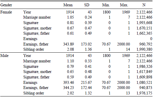
Table 1 presents summary statistics from the dataset. The main unit of observation is a marriage, linked to both the groom’s and the bride’s parents. Each observation contains, when available, information about the human capital of the bride, the groom, and all four parents. In the rest of this section, I discuss in detail how the links were constructed, what measures of human capital I use, and how reliably the data report these measures for women.
SUMMARY STATISTICS

Notes: Each observation is a marriage, with marriage number the number of the marriage for the relevant participant. Signature variables are indicators that are one if a signature was recorded, zero if the absence of a signature was recorded, and omitted otherwise. Earnings are the imputed annual earnings for the individual’s occupation in 1901 Canadian dollars (see text). Sibling order is the order among all married siblings by date of first marriage (as birthdates are not reported after 1849).
Source: Project BALSAC (Reference BALSAC2020).
Linked Family Vital Records
Two unusual institutional features of Quebec have resulted in vital records that are particularly easy to link. First, due to the system of community property, both husbands and wives signed their names on all legal documents. Second, women kept their family names when they married. This means both that women can be linked to their fathers and that most vital records have four names on which to link (the first names and last names of both the husband and wife or mother and father).
The vital records in the database have been reconstituted into families using computer-assisted linkage. The links are almost entirely based on names, with dates being used to validate links after they are formed (Vézina and Bournival Reference Vézina and Bournival2020; Vézina, Bournival, and Bellavance Reference Vézina, Marc St-Hilaire and Bellavance2018). Names are standardized using the FONEM phonetic program (Bouchard, Brard, and Lavoie Reference Bouchard, Brard and Lavoie1981). Manual linkage is used in around 20 percent of cases where there is no unique match. Manual linkages are not necessarily better than automatic linkages; in some applications, they produce both more true matches and more false positives (Abramitzky et al. Reference Abramitzky, Boustan, Eriksson, Feigenbaum and Pérez2021). However, the fact that the Quebec vital records have four names to match on should increase the accuracy of matching, regardless of the method used. Moreover, the parish records of Quebec have survived remarkably intact, as local priests were required to send duplicates of all records to their superiors (Dillon et al. Reference Dillon, Amorevieta-Gentil, Caron and Lewis2018). Therefore, records of almost the entire population survive; this will reduce false positive rates in an analogous way to the linking of full-count to full-count censuses (Abramitzky et al. Reference Abramitzky, Boustan, Eriksson, Feigenbaum and Pérez2021).
Measures of Human Capital
The direct measure of human capital that I use in this paper, for both men and women, is the presence of a signature on a marriage record. Signatures have often been used as a proxy for literacy (A’Hearn, Baten, and Crayen Reference A’Hearn, Baten and Crayen2009). In Quebec, Catholic churches had long required both the bride and the groom to sign their marriage records if they were able; the priest was required to record if they were not (Gagnon et al. Reference Gagnon, Tremblay, Vézina and Seabrook2011). I code a signature variable as one if the individual signed their marriage record and zero if they were unable to sign. I omit signatures that are either missing or unrecorded (see Online Appendix 1 for details on the raw literacy variable). As shown in Figure 1, this definition produces a trend that is close to external estimates of literacy.
THE VITAL RECORDS ACCURATELY REPORT THE ABILITY TO WRITE
Notes: The vital records are from the BALSAC database. For the vital records, literacy is proxied by a signature variable that is one if a signature was recorded, zero if the absence of a signature was recorded, and omitted otherwise. The census literacy rate is the fraction of individuals who were reported as able to write, reweighted to match the age distribution in the vital records. The two sources broadly agree.
Sources: Canadian Families Project (2002), Gaffield et al. (Reference Gaffield, Baskerville, Cadigan, Marc St-Hilaire, Normand, Darroch, Amhrein, Tepperman, Jones and Sager2009), Inwood and Jack (Reference Inwood and Jack2011), Minnesota Population Center (2019), and Project BALSAC (Reference BALSAC2020).

Was literacy human capital in the sense of increasing economic productivity? The qualitative evidence suggests it was. The ability to write had always been associated with business activity in Quebec (Greer 1997). Online Appendix 1 shows the 20 most common occupations for men in the nineteenth century. Signature rates range widely with a clear occupational hierarchy. Skilled professionals and merchants were highly likely to sign, craftsmen were somewhat less likely to sign, and workers in the primary sector were far less likely to sign. As for reading, it too was likely associated with economic activity. As opposed to their Protestant neighbors who prioritized literacy education for religious ends, Quebec’s Catholics would have considered reading the Bible a virtue but not a necessity.
A second proxy for human capital, only reliably available for men, is occupational status. I assign each individual the occupation listed at their first marriage (if any). The occupations are assigned HISCO codes, a classification system designed for comparative studies of historical social mobility (Van Leeuwen, Maas, and Miles Reference Van Leeuwen, Maas and Miles2004). I then assign various occupational status scores to these HISCO codes. My scores of choice are imputed 1901 earnings. I construct them using a 5 percent sample of the 1901 Canadian Census for a given occupation (Canadian Families Project 2002; Minnesota Population Center 2019). For each occupation, I simply take the average yearly earnings reported by men in Quebec.Footnote 10 There are numerous other ways to rank occupations, as discussed in Online Appendix 2. However, imputed 1901 earnings have several advantages. First, they are easy to interpret: they are how much the individual would earn, on average, with their occupation in 1901 in Quebec. Second, they are imputed from data roughly in the middle of the time period considered. Third, they are at least a proxy for the standard variable of interest in intergenerational mobility studies (lifetime earnings). Fourth, they produce similar estimates to the other occupational scores. Finally, the average earnings of an occupation were strongly related to the average level of human capital of those in the occupation. Therefore, the main results in this paper use the imputed 1901 earnings as the primary measure of occupational status.
Reporting of the Characteristics of Women
Do the vital records in the BALSAC database accurately report literacy of women? The Canadian Censuses of 1891, 1901, and 1911 recorded whether individuals could read and write (Canadian Families Project 2002; Dillon Reference Dillon2008; Gaffield et al. Reference Gaffield, Baskerville, Cadigan, Marc St-Hilaire, Normand, Darroch, Amhrein, Tepperman, Jones and Sager2009; Inwood and Jack Reference Inwood and Jack2011; Minnesota Population Center 2019).Footnote 11 Figure 1 compares the fraction of individuals who signed their first marriage record to the fraction who self-reported the ability to write in the censuses. Unlike the censuses, individuals only appear in the marriage records during a specific time in their lives. To account for this, I reweight the census data to match the age distribution of the BALSAC vital records. As shown in the figure, my estimated literacy rate closely tracks the rate in the censuses. Two patterns are particularly notable. First, Quebec transitioned from a very low level of human capital to a fully literate society between 1800 and 1920. Second, there was a gender gap in favor of women between 1850 and 1920.Footnote 12
While occupational status gives a more detailed measure of socioeconomic status, it is not observed for most women in the BALSAC vital records (Online Appendix 3). Thus, I take two approaches. When possible, I use signature literacy to directly observe women. However, this does not work well for estimating the degree of assortment over time. Therefore, I develop a new method to estimate the degree of assortment from the observed occupational statuses of the groom, his father, and his father-in-law.
METHODS
I develop a new method to measure the degree of marital assortment. Using this method, I show in the following section that assortment was surprisingly high and stable over the period of 1830–1969. This ratio method, first developed in an early version of this paper, has since been extended to other contexts. Clark and Cummins (Reference Clark and Cummins2022) similarly find a degree of assortment of 0.8–0.9 in England from 1837–2021. Clark, Cummins, and Curtis (Reference Clark, Cummins and Curtis2022) adapt the method to estimate rates of intergenerational mobility. Finally, Luo (Reference Luo2022) develops a similar model for Imperial China from 1614–1854 under the assumption that matching is solely between the father and father-in-law.
Following Espín-Sánchez, Gil-Guirado, and Vickers (Reference Espín-Sánchez, Gil-Guirado and Vickers2022), I adapt a simple model to illustrate how assortative marriage and intergenerational mobility contribute to inequality over the long run. This model implies that assortment matters for mobility if spouses match on socioeconomic status (henceforth, “status”) and that mothers have a direct, independent effect on the outcomes of their children. Later, I find empirical support for both conditions, suggesting that the high measure of assortment will have mattered for social mobility.
Ratio Method
Chadwick and Solon (Reference Chadwick and Solon2002) observe that if the elasticity between a woman’s income and that of her parents is very similar to the elasticity between her husband’s income and that of her parents, then assortment plays a major role in intergenerational mobility. In this section, I build on this insight to develop a new method for directly estimating the degree of assortment between spouses.
While the method requires assumptions about underlying causal relationships, what it estimates is the correlation in status between the bride and groom. The advantage of this method is that it only requires measuring the correlation in status between a groom and his father and between a groom and his father-in-law. In Online Appendix 4, I discuss extensions to this method that use the correlation between the father and father-in-law.
BASELINE VERSION
For simplicity, I first derive the ratio method assuming there is no measurement error. Later, I add classical measurement error; that is, I consider the case when only imperfect measures of the other status variables are available.
For each couple i, let B i be the status of the bride, G i be the status of the groom, FB i be the status of the bride’s father, and FG i the status of the groom’s father. Note that B i is not observed in the data. First, assume that the variance of status is the same for brides and grooms:
Assumption 1 Equal variance: Var(B i) = Var(G i)
Let γ be the Pearson’s correlation coefficient between the statuses of spouses: $Corr({B_i},{G_i}) = \gamma $
Using Assumption 1 and the definition of Pearson’s correlation coefficient, this can be written as a linear equation, which can be estimated by simple least squares regression. To illustrate why, note that for any x and y, the simple regression of y on x results in coefficient $\beta = {{Cov(x,y)} \over {\sigma _x^2}}$
.
$\beta = {{Cov(x,y)} \over {\sigma _x^2}}$
.
Pearson’s correlation is $\rho = {{Cov(x,y)} \over {{\sigma _x}{\sigma _y}}}$
. Thus,
$\rho = {{Cov(x,y)} \over {{\sigma _x}{\sigma _y}}}$
. Thus, $\beta = \rho {{{\sigma _y}} \over {{\sigma _x}}}$
and, if σ y = σ x, then β = ρ. This is not a causal relationship; it is merely writing the correlation in a linear form. Also, note that the residuals in this OLS regression will be uncorrelated with the independent variable by construction. The linear form of the correlation is thus:
$\beta = \rho {{{\sigma _y}} \over {{\sigma _x}}}$
and, if σ y = σ x, then β = ρ. This is not a causal relationship; it is merely writing the correlation in a linear form. Also, note that the residuals in this OLS regression will be uncorrelated with the independent variable by construction. The linear form of the correlation is thus: ${G_i} = \gamma {B_i} + {\varepsilon _i}$
Second, assume that the correlation between fathers and children is β regardless of the gender of the child:
Assumption 2 Symmetric inheritance: Corr(FG i, G i) = Corr(FB i, B i) = β
Using Assumption 2, the intergenerational association of status is: $Corr(F{B_i},{B_i}) = \beta ,$
which can similarly be written linearly as: ${B_i} = \beta F{B_i} + {\upsilon _i},$
and likewise for grooms: ${G_i} = \beta F{G_i} + {\mu _i}$
Substituting Equation (4) into Equation (2): ${G_i} = \gamma \beta F{B_i} + \gamma {\upsilon _i} + {\varepsilon _i}$
Finally, assume that the assortment between spouses is based only on their status, not that of their parents. That is, assume that the status of a groom is uncorrelated with the status of his father-in-law, conditional on the status of his bride.
Assumption 3 Direct assortment: Corr(FB i, ε i) = 0
Note FB i and υ i are uncorrelated by construction. Now consider two regressions: ${G_i} = {\rho _1}F{G_i} + {e_i}$ ${G_i} = {\rho _2}F{B_i} + {u_i}$
If we estimate Equations (7) and (8), we get estimates ${{\hat \rho }_1}$
of β and
${{\hat \rho }_1}$
of β and ${{\hat \rho }_2}$
of γβ. Assumption 3 is necessary for
${{\hat \rho }_2}$
of γβ. Assumption 3 is necessary for ${{\hat \rho }_2}$
to be an unbiased estimate. The ratio
${{\hat \rho }_2}$
to be an unbiased estimate. The ratio ${{\hat \rho }_2} / {{\hat \rho }_1}$
is thus an estimate of γ. Confidence intervals can be constructed using bootstrapping.
${{\hat \rho }_2} / {{\hat \rho }_1}$
is thus an estimate of γ. Confidence intervals can be constructed using bootstrapping.
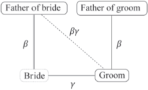
Figure 2 shows the setup of the ratio method as a diagram. The solid nodes represent observed variables, and the dashed node represents an unobserved latent variable (the brides’ status). Solid lines represent a direct link between individuals. These direct links involve underlying causal relationships, such as intergenerational inheritance or the process of assortment between spouses. These causal mechanisms likely involve other individuals, notably mothers (as discussed next). However, we assume no direct causal link between the groom and his father-in-law, as indicated by the dashed line. There is a causal pathway between the two, but it runs only through the bride. Variables represent the correlations between nodes.
RATIO METHOD
Notes: Solid nodes represent observed variables. Dashed nodes represent unobserved latent variables. Solid lines represent a direct link. Dashed lines represent an indirect link. Variables represent the correlations across a link.
Source: Author’s illustration.

ADDING CLASSICAL MEASUREMENT ERROR
In practice, all measures of socioeconomic status are imperfect. Assuming each latent (true) variable X is observed with classical measurement error e X, the estimates from Equations (7) and (8) will both be attenuated downwards by factors θ 1 and θ 2: ${\rm{plim}}\,\,{{{\rm{\hat \rho }}}_{\rm{1}}} = {{\sigma _{F{G_i}}^2} \over {\sigma _{F{G_i}}^2 + \sigma _{{e_{F{G_i}}}}^2}}{\rho _1} = {\theta _1}\,\beta $ ${\rm{plim}}\,\,{{{\rm{\hat \rho }}}_{\rm{2}}} = {{\sigma _{F{B_i}}^2} \over {\sigma _{F{B_i}}^2 + \sigma _{{e_{F{B_i}}}}^2}}{\rho _2} = {\theta _2}\,\lambda \beta $
The ratio method will be robust to this classical measurement error under two additional assumptions:
Assumption 4 Equal variance 2: Var(FG i) = Var(FB i)
In other words, assume the variance of status is the same for fathers of brides and fathers of grooms.
Assumption 5 Equal measurement error: Var(e FBi) = Var(e FGi)
In other words, assume the fathers of brides are measured with the same measurement error as the fathers of grooms.
By Assumptions 4 and 5, θ 1 = θ 2. Thus, the ratio ${{\hat \rho }_2} / {{\hat \rho }_1}$
is still an unbiased estimator of γ. This result, while relying on rather strict assumptions, is based on straightforward intuition: we attenuate downwards both the numerator and denominator of the ratio by the same amount, leaving the ratio itself unchanged.
${{\hat \rho }_2} / {{\hat \rho }_1}$
is still an unbiased estimator of γ. This result, while relying on rather strict assumptions, is based on straightforward intuition: we attenuate downwards both the numerator and denominator of the ratio by the same amount, leaving the ratio itself unchanged.
DISCUSSION OF ASSUMPTIONS
To review, the key assumptions for the ratio to be equal to the degree of assortment are as follows. First, equal variances of true status. Second, symmetric inheritance: true status is inherited at the same rate regardless of whether the child is male or female. Third, direct assortment: assortment is based solely on the true status of the bride and groom. Fourth, equal attenuation bias: the measurement error is the same for the correlation between grooms and their fathers and for the correlation between grooms and their fathers-in-law.
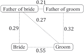
Figure 3 shows that the observed correlations of signatures are, when allowing for some imprecision in the estimates, consistent with the symmetric inheritance assumption. Later, I find additional evidence that it is reasonable my context. Of course, there may be other assumptions that would be consistent with this pattern. Moreover, once we consider measurement error, the equal inheritance assumption relates to the latent true status, which we do not directly observe. Thus, symmetric inheritance remains, by necessity, an assumption.
OBSERVED SIGNATURE CORRELATIONS
Notes: Signature variables are indicators that are one if a signature was recorded, zero if the absence of a signature was recorded, and omitted otherwise. Dashed lines represent an observed correlation.
Source: Project BALSAC (Reference BALSAC2020).

The equal attenuation bias assumption is discussed previously in terms of classical measurement error. One important way in which the errors can be non-classical is if ε i is correlated with FB i. That is, if the matching equation between the bride and groom has an omitted variable bias from the status of the father-in-law. This would be the case if the status of the groom is matched directly to that of his father-in-law, as well as that of his bride. In other words, this is another reason why we must assume direct assortment.
Figure 3 shows that the observed correlations of signatures are consistent with this assumption. The correlation is stronger between the bride and groom than between the groom and father-in-law or the father and father-in-law. Again, there may be other assumptions that would be consistent with this pattern, so direct assortment is still necessarily an assumption.
How plausible is the direct assortment assumption? Arranged marriages are not a problem if those doing the arranging only consider the status of the bride and groom. This assumption is only violated if the statuses of the groom’s in-laws are considered independently of the status his bride has inherited. With a flexible definition of status, it is hard to come up with an example of a violation of this assumption. For example, if an elite family’s daughter marries well because she benefits from her family’s wealth or social connections, this could be considered part of her socioeconomic status, which she has inherited.
EMPIRICS
The following section outlines the three main empirical findings of this paper. First, I use the ratio method derived in the previous section to estimate the degree of assortment over time. This estimate is high and stable throughout the period. Second, I show that assortment was due to sorting on individual characteristics, not the spurious result of matching between families. Third, I provide evidence that suggests mothers directly affect the outcomes of children. Together, these provide evidence that this high degree of assortment decreased social mobility. Parents closely matched on their individual traits, which, in turn, had independent effects on child outcomes. (I formally describe this intuition with a simple model in Online Appendix 5). The code to replicate these analyses is available online (Curtis 2025).
Measuring the Degree of Marital Assortment
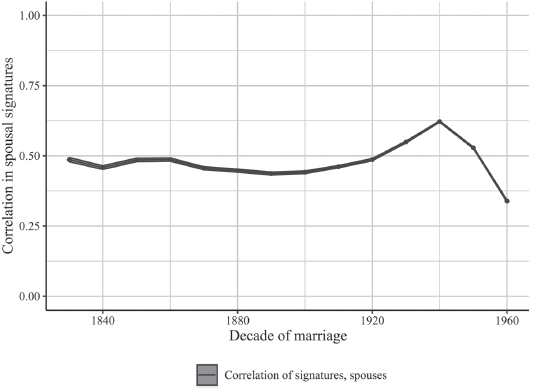
Did the degree of assortment for marriages change over time? Figure 4 plots the correlation of spouses’ literacy, proxied by signatures. The degree of assortment appears to be relatively stable throughout the nineteenth century and an inverted-U shape in the twentieth century. However, there are good reasons to be skeptical of this simple measure. The ability to sign one’s name is a relatively low bar. An individual who passes that threshold could be barely literate or have many years of schooling. In effect, signature rates are a highly right-censored measure of human capital. As the population approaches near-universal literacy in the early twentieth century, this censoring will obscure most of the variation in human capital. A second issue is that, even under perfect assortment, if the average signature rate for men and women is different, then the maximum correlation is not one (Liu and Lu Reference Liu and Lu2006). This maximum correlation changes over time, so how close the observed correlation is to the maximum also changes. In short, Figure 4 is not a satisfactory measure of assortment.
CORRELATION OF SPOUSES’ SIGNATURES
Notes: Ninety-five percent confidence interval shaded. Y-axis is the Pearson’s correlation coefficient. Signature variables are indicators that are one if a signature was recorded, zero if the absence of a signature was recorded, and omitted otherwise.
Source: Project BALSAC (Reference BALSAC2020).

As described in the previous section, an alternative measure can be constructed by comparing the correlation of the status of sons-in-law and fathers-in-law to that of sons and fathers. The former are two degrees separate: an intergenerational link from father-in-law to daughter and a marriage link from daughter to son-in-law. The latter has only one degree of separation: an intergenerational link from father to son. I show that, with some assumptions, the ratio of the correlations is equivalent to the degree of assortment. The key assumptions in the model are that children inherit status equally regardless of gender and that the father-son correlation has the same measurement error as the father-in-law-son-in-law correlation. I argue that these strong assumptions have empirical support in this specific context. Online Appendix 6 shows some evidence that grooms did not match directly with their fathers-in-law. In the third set of empirical results, I show that inheritance of human capital is symmetric across genders.
For my preferred measure of occupational status, I use the imputed annual earnings in 1901 Canadian dollars. To normalize the standard deviations, I compute Spearman’s rank correlation coefficients, which are equivalent to estimating the canonical rank-rank mobility regressions (Chetty et al. Reference Chetty, Hendren, Kline and Saez2014).
Figure 5 plots the ratio measure over time (see Online Appendix 7 for the underlying correlations). The estimated correlation between spouses is very high, around 0.8, and it appears to be stable throughout the period. The overall trend is similar to that in Figure 4 before the mid-twentieth century. However, as mentioned, literacy is both a noisy measure of human capital and becomes much less informative as the average level of education grows. Together, I interpret the two figures as consistent with a story where the degree of assortment is high and stable throughout the entire period.
RATIO MEASURE OF MARTIAL SORTING USING IMPUTED EARNINGS
Notes: ninety-five percent bootstrapped confidence intervals shaded (10,000 replications). imputed earnings are the imputed annual earnings for the individual’s occupation in 1901 canadian dollars (see text). spearman’s rank correlations are used, which is equivalent to the correlation of the ranks.
Source: project balsac (2020).

Online Appendix 8 presents several robustness checks for the estimation of the degree of assortment over time. The ratio can then be computed. I use alternative measures of occupational status, use the error correction method from Nybom and Stuhler (Reference Nybom and Stuhler2017), simulate within-occupation error in the spirit of Espín-Sánchez et al. (2019), and simply compare fathers and fathers-in-law as done by Craig et al. (Reference Craig, Eriksson, Niemesh and Rashi2023). The overall conclusion is the same.
Did Spouses Match on Individual Human Capital?
One can imagine a society in which marriage matches were not based on the human capital of the brides. For example, marriages could be negotiated to form an alliance, with the characteristics of the wife an afterthought at best (Puga and Trefler Reference Puga and Trefler2014).Footnote 13 In this hypothetical society, there would still be an observed correlation in the human capital of spouses if a woman’s human capital is partially determined by her father.
To test if individual characteristics mattered, consider the following fixed effects regression: ${G_{i,BF}} = \alpha {B_{i,BF}} + {\phi _{BF}} + \beta {X_{i,BF}} + {\varepsilon _{i,BF}},$
where B i,BF is a characteristic of bride i from family BF, G i,BF is the characteristic of her spouse, φ BF are the crucial fixed effects that control for the bride’s family background, X i,BF is a vector of controls, and ε i,BF, is an error term. To address any time trends, X i,BF can include fixed effects for both decade and the order of siblings.Footnote 14
In other words, the regression asks if, compared to her siblings, a woman with more human capital marries a man with more human capital. If so, α will be positive.
As shown in Table 2, Panel A, a woman who signed her marriage record married a man with more human capital than her sisters who did not. Being able to write was associated with an increase in the probability that a woman’s husband was literate by 34 percentage points. This is evidence that marriage matches were based on individual characteristics.
FAMILY FIXED EFFECTS, LITERATE SPOUSE

Notes: *p<0.10; **p<0.05; ***p<0.01. Family-clustered standard errors in parentheses. The sample excludes individuals with one or more unknown parents. Signature variables are indicators that are one if a signature was recorded, zero if the absence of a signature was recorded, and omitted otherwise. Column (2) is my preferred specification. In Column (3), to illustrate the size of the identifying variation, the sample is restricted to just families where at least one sibling signed and one did not. Note that after adding family fixed effects the estimates are close to symmetrical across genders.
Source: Project BALSAC (Reference BALSAC2020).
Note that while the family fixed effects do reduce α ^ , this does not reveal the degree to which matches are coordinated by families. If matching is only on individual characteristics, the family fixed effects will still reduce α ^ as long as the human capital of sisters is correlated. This reduction can be very large, as the human capital of siblings is often highly correlated. The fixed effects will, essentially, leave only the component of the bride’s human capital uncorrelated with that of her siblings. The estimated coefficient of the human capital of a bride is potentially only a small part of the true effect. The relevant null hypothesis is thus whether the coefficient is zero.
What about men and their brothers? As shown in Table 2, Panel B, men who were able to write also married better. Being able to write was associated with an increase in the probability that a man’s wife was literate by 32 percentage points. This estimate is similar to that for women. The returns to human capital for marriage matching appear to be the same, regardless of gender.
What is the economic significance of matching on the individual characteristics of women? If it were not the case, the woman’s family could, after all, still matter for the outcomes of her children. First, the results show that there was a return to education for women in terms of the economic status of the household she formed at marriage. This was the case even if she did not employ her human capital in a formal occupation. Second, it implies a stronger role for assortative marriage in intergenerational mobility, assuming mothers mattered directly for their children’s outcomes. Finally, it hints that women may have had some agency over the marriage matching process.
Online Appendix 9 presents several robustness tests. First, I estimate similar regressions using occupational status instead of literacy. Second, I estimate a selection into identification model, which accounts for the fact that families with one literate and one illiterate child are perhaps atypical (Miller, Shenhav, and Grosz Reference Miller, Shenhav and Grosz2023).
Do Mothers Matter Directly for Child Outcomes?
For assortment to matter for social mobility, mothers must have a direct effect on child outcomes. A mother’s literacy is associated with that of her children, even after controlling for that of the father (Table 3, Panels A and B, Column (1)). Notably, there appears to be no difference between the associations with children of different genders.Footnote 15 However, this pattern could still be observed if the mother did not directly matter for the outcomes of the children. With assortment, if the husband’s ability is observed with measurement error, the mother’s ability would be correlated with the residual even if its true effect is zero. Therefore, simple regressions controlling for the literacy of fathers do not identify the effect of the abilities of mothers.
PARENTAL AND CHILD HUMAN CAPITAL, SECOND PARENT FIXED EFFECTS

Notes: *p<0.10; **p<0.05; ***p<0.01. Family-clustered standard errors in parentheses. The sample excludes individuals with one or more unknown parents. Signature variables are indicators that are one if a signature was recorded, zero if the absence of a signature was recorded, and omitted otherwise. In Columns (4) and (5), to illustrate the size of the identifying variation, the sample is restricted to just parents who had at least one spouse who signed and one who did not. Controls include marriage year and sibling marriage order fixed effects (as birthdates are not reported after 1849).
Source: Project BALSAC (Reference BALSAC2020).
To identify a causal effect, ideally, we would control for the father but randomize the mother. A less ideal (yet possible) approach is to consider the case where a father has children from more than one marriage. However, this results in three complications. The first is the chance that the children are scarred by whatever event resulted in a second marriage (likely a death). Assuming this penalty is a constant, it can be controlled for by including fixed effects for the number of the marriage the children are from. Second, the death of a spouse is not a random event. It is possible, though highly unlikely, that only women who remarry have a direct impact on children. Third, as marriage is assortative based on the abilities of mothers, the abilities of each wife of the father will be correlated. Therefore, similar to the family fixed effects noted earlier, the father fixed effects will absorb part of the effect of the mother’s ability. Indeed, if the degree of assortment is high, most of the effect of the mother will be absorbed. Again, the estimated coefficient for the human capital of the mother is potentially only a small part of the true effect. The relevant null hypothesis is thus whether the coefficient is zero. I regress: ${C_{i,F}} = \alpha M{C_{i,F}} + {\phi _F} + {\delta _{ma{r_F}}} + { \in _{i,F}},$
where C i,F is an outcome of a child i with father F, MC i,F is a characteristic of the child’s mother, φ F are the crucial fixed effects that control for the father, δ marF are fixed effects to control for the marriage number of the father, and ε i,F is an error term.
As shown in Table 3, even controlling for the father, a mother who could sign her name had children who were 1–3 percentage points more likely to be able to sign their names. This direct independent effect, while statistically significant, appears to be very small. However, as shown previously, the human capital of spouses is highly correlated. The father fixed effects will control for most of the characteristics of his wives. Even if one can sign her name and the other cannot, they are likely otherwise very similar, and the father fixed effects control for that similarity. In other words, after controlling for the father fixed effects, there is only a small residual amount of variation, but it is directly attributable to the mother. Again, the relevant null hypothesis is whether the coefficient is zero.
I also estimate the effects of the ability of a father, controlling for the mother. Notably, the results are very similar to those of the regressions for mothers. Once the correlation between the abilities of spouses is accounted for through fixed effects, the direct independent effect of parental human capital appears to be symmetrical across the genders of both the parent and the child. This is reassuring, as the ratio method developed earlier in this paper assumes that children inherit human capital from their fathers at the same rate regardless of gender. In Online Appendix 10, I estimate similar results using occupational status.
DISCUSSION
The empirical findings of this paper demonstrate that marriage was strongly assortative in the past, with direct consequences for intergenerational mobility. As I argued earlier, these findings for Quebec are generalizable to other populations. This has several implications for the standard approaches to studying intergenerational mobility. In Online Appendix 11, I discuss how overlooking mothers and marriage can lead to misleading conclusions when looking at both father-son intergenerational correlations and the role of grandfathers.
CONCLUSION
In this paper, I construct a simple model of marriage and mobility. It shows that even in the absence of female participation in the labor force, assortative marriage will increase inequality if the ability of a woman determines whom she marries and the success of her children. To test if this was true in Quebec from 1800–1970, I consider a novel dataset containing millions of families reconstructed from vital records. Unusually, married women are linked to their fathers; I use this to develop a new ratio method to estimate the degree of assortment, finding it surprisingly high and stable over time. Next, I find pairs of sisters where only one was able to sign her name. I show that the more educated sister still typically earned an education premium when it came to the socioeconomic status of her husband. Moreover, I show her ability mattered as much as her husband’s for the outcomes of their children. As quick remarriage after losing a spouse was the norm, I hold one parent constant and allow the second to vary. Sharing a mother mattered as much as sharing a father for child outcomes. Altogether, I conclude that assortative marriage has always mattered for inequality. It mattered because, despite severe legal and economic disadvantages, women played a major role in mobility and marriage. Overlooking the role of women and marriage would leave our understanding of intergenerational mobility and inequality in the long run incomplete.


 Open access