


The Reconstruction Finance Corporation (RFC) was created by President Hoover in early 1932 during the depths of the Great Depression. The objective of the RFC was to “make temporary advances upon proper securities to established industries, railways, and financial institutions which cannot otherwise secure credit, and where such advances will protect the credit structure and stimulate employment” (hereafter referred to as “the twin objectives”) (RFC 1959, p. 1). The Corporation approved $3.9 billion in loans from 1932 until 1939.Footnote 1 We call such loans “bailouts” because they were provided at below-market interest rates to companies struggling to access commercial credit.Footnote 2 Although most of these loans went to the financial sector (see, e.g., Mason Reference Mason2001; Calomiris et al. Reference Calomiris, Mason, Weidenmier and Bobroff2013; Butkiewicz Reference Butkiewicz1995, Reference Butkiewicz1997), railroads were, by far, the largest non-financial sector recipient (i.e., $1.17 billion, including rollovers) during this eight-year period. In this paper, we explore how the RFC’s bailouts for railroads and limited assistance from the Public Works Administration (PWA) impacted the economy.
Our results suggest that RFC loans to railroads may have had limited success in achieving their primary stated objectives of increasing employment and preventing defaults. However, the program is estimated to have had other notable effects, including increasing worker wages and providing positive spillovers to manufacturing firms located along railroad routes. Bailouts also allowed loan recipients to slightly reduce leverage, and there was a significant increase in bond prices following the announcement of a loan application or approval. Indeed, in the nine days surrounding news of an application, bailed-out railroads’ bond prices experienced, on average, an abnormal return (AR) of 2.2 percent. An approval is associated with a 1.8 percent abnormal return for bonds, but a negative effect on equity prices. Bailouts appear to have benefited existing employees and bondholders rather than aiding firm performance, such as railroad profits.
Second, we study the impact of railroad bailouts on the broader economy. Although New Deal railroad assistance was not explicitly aimed at the railroads’ customers, we find that firms located in the same city or town as a bailed-out railroad experienced positive spillovers from news of a forthcoming railroad loan. Manufacturing firms whose operations had a high geographical overlap with the assisted railroad experienced a 1.0 percent abnormal return upon the announcement of the bailout, compared to a 0.4 percent abnormal return for manufacturers with low levels of overlap with that railroad.
Railroads were a vital part of the U.S. economy in this era. The transportation sector employed over 3 million people in 1929 (6.9 percent of total employment) and generated $6.6 billion of national income (8.2 percent of total income), see Kuznets (Reference Kuznets1934). Railroads comprised about 13 percent of the New York Stock Market in January 1929, and the Great Depression hit the railroad sector particularly hard.
Details of government railroad loans were quickly made public by the railroad regulator, the Interstate Commerce Commission (ICC), and widely reported in the media. It was, by contrast, impossible to observe the immediate impact of government loans in most sectors during the Great Depression. Loans to banks, farms, and industrial firms were largely kept secret, and financial claims on these firms were not usually traded in liquid financial markets. Anbil (Reference Anbil2018) shows that banks that unexpectedly had their loans from the government revealed in August 1932 experienced drops in deposits of 18 to 25 percent compared to control banks. These banks were also 78 percent more likely to fail after their loans were publicly disclosed.
Government loans to railroads required approval by both the RFC and the ICC. The New York Times reported on 21 May 1932 that (p. 21), “although the corporation (RFC) cannot approve loans unless they are sanctioned by the (ICC) commission, it is not required to make the advances sanctioned.” A government loan required eight conditions to be met: (i) that the applicant could not obtain funds on reasonable terms from banks or the public, (ii) approval of the ICC, (iii) a maturity of less than three years, (iv) that the borrower existed prior to 1932, (v) total government loans to the applicant were less than $100 million, (vi) no fees or commissions were paid by the applicant, (vii) that the applicant consents to examinations by the ICC or other authorities, and (viii) collateral must meet the terms of the Finance Corporation act.Footnote 3 The ICC, as the regulator, was required to approve most changes to a railroad’s operations (e.g., terminating a line, capital expenditure) or financing arrangements, such as issuing additional debt.
In total, 205 railroad applications (from 50 railroads) were successful, 32 applications were rejected, and 14 applications were subsequently withdrawn. Railroads that obtained a government loan likely differed from railroads that did not receive government aid. Although we condition our results on the publicly available characteristics of railroads, it is likely that railroads also differed along unobservable dimensions. To address this issue, we take advantage of the political process that was inherent in RFC decision-making. That is, RFC directors were appointed by the President and confirmed by the U.S. Senate. Political considerations were allegedly important in the “New Deal” decision-making process, see, for example, Wright (Reference Wright1974), Wallis (Reference Wallis1987), and Fishback, Kantor, and Wallis (Reference Fishback, Kantor and Wallis2003). Kroszner (Reference Kroszner1994) finds some evidence of political influence on the RFC’s decision-making; however, Mason’s (Reference Mason2003) study of the RFC bank program shows little evidence of political interference. We find that railroad bailouts were more likely to be granted to railroads that operated in the home states of RFC directors. Using the composition of the RFC board as an instrument for government assistance, we fail to find any beneficial effects on railroad employment or the likelihood of bond defaults.
Direct government aid to the real economy has rarely been attempted during a crisis, although direct aid was a big part of many governments’ COVID-19 responses (see, e.g., Cirera et al. Reference Cirera, Cruz, Davies, Grover, Iacovone, Cordova, Medvedev, Maduko, Nayyar, Ortega and Torres2021; Elenev, Landvoigt, and Van Nieuwerburgh Reference Elenev, Landvoigt and Van Nieuwerburgh2022; Granja et al. Reference Granja, Makridis, Yannelis and Zwick2022).Footnote 4
Non-financial firms experience a crisis differently than banks. There can be no “runs” on a railroad’s assets, in contrast to banks. U.S. railroads, for instance, often issued 50-year bonds to finance their operations (see Benmelech, Frydman, and Papanikolaou Reference Benmelech, Frydman and Papanikolaou2019). Railroads cannot quickly change their operations to “gamble on resurrection” (see, e.g., Hellmann, Murdock, and Stiglitz Reference Hellmann, Murdock and Stiglitz2000; Dewatripont and Tirole Reference Dewatripont and Tirole2012). Tracks and other real assets are fixed and costly to divert in the search for new business.
The Great Depression and the Reconstruction Finance Corporation
The Great Depression was an unprecedented period of economic and financial collapse worldwide. It struck the United States particularly severely, with peak-to-trough industrial output falling 40 percent by late 1931 and GDP still 25 percent below trend six years after the recovery began (see Cole and Ohanian Reference Cole and Ohanian2004; Ohanian Reference Ohanian2009). There were several waves of banking crises in the early 1930s (see Bernanke Reference Bernanke1983; Friedman and Schwarz 1963). In response to the weak economy and runs on troubled banks, President Hoover reluctantly created the RFC in January 1932, which was a component of what came to be known as the “New Deal.” The RFC was initially permitted to loan to financial firms and railroads; loans were later permitted for farms, state and local governments, infrastructure projects, and industrial firms. The RFC’s initial capital stock came from a $500 million appropriation from the Treasury. While it obtained the bulk of its additional funding by issuing notes to the Secretary of the Treasury, a tiny part of its operations was provided for by direct borrowing from the public.
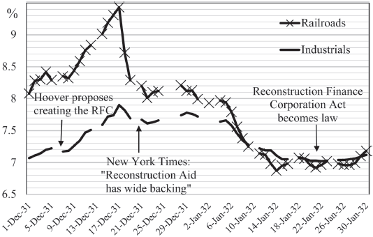
Hoover argued, in his State of the Union address on 8 December 1931, that railroads’ “prosperity is interrelated with the prosperity of all industries.” The New York Times reported on 19 December 1931, that Hoover believed that “the plight of the American railroads is only temporary and that they will be able to work themselves out of the depression.”Footnote 5 The United States had experienced severe railroad defaults during crises in 1873, 1884, and 1893, in which multiple large lines defaulted, resulting in significant drops in railroad employment (see Schiffman Reference Schiffman2003; Giesecke et al. Reference Giesecke, Longstaff, Schaefer and Strebulaev2011; Cotter Reference Cotter2021). The chairman of the ICC was reported in December 1931 as being in favor of government loans to railroads.Footnote 6 Once a policy of government support for railways became clear, in December 1931 and January 1932, railroad bond yields declined markedly relative to unsupported industrial bond yields (see Figure 1). Indeed, the government’s announced policy of providing support for the railroad industry may have had a larger beneficial impact on the industry than the loans granted to individual companies. The policy may have increased business confidence and encouraged railroad creditors to grant more forbearance on outstanding loans.
MOODY’S BOND YIELDS
Source: Commercial & Financial Chronicle (various issues).

Railways were hard hit in the early years of the Depression. The net income of class 1 railways fell from $896 million in 1929 to just $6 million in 1933 and never fully recovered. Net income was still below $200 million by the start of WWII. By the end of 1932, over 22,000 miles of railroad were in the hands of receivers, up from 5,700 miles at the end of 1929.Footnote 7 An initial attempt to solve the railroad sector’s problems was the creation of the Railroad Credit Corporation (RCC) in late 1931 (see Spero Reference Spero1939, pp. 16–17). The ICC allowed railroads to increase their freight rates, and part of the increased revenue would be “extended by the pool to weak lines in the form of loans.”Footnote 8 The chairman of the New York, New Haven, and Hartford Railway acted on behalf of the Association of Railway Executives in administering the RCC’s loan program. This corporation made loans of $73.6 million to railroads from early 1932 until May 1933 (see Spero Reference Spero1939, pp. 16–17).
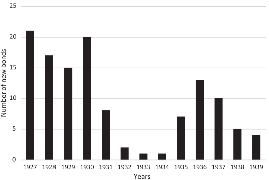
Part of the rationale for providing aid to railroads was that many railroads could not repay their maturing bonds, and it would be exorbitantly expensive for them to obtain alternative funding from the banking sector. In late 1931, Daniel Willard testified in the Senate that railroads “cannot borrow money from banks at less than 8 or 9 percent interest,” when most maturing bonds had coupon rates of around 4 percent.Footnote 9 The bond market for railroads virtually closed during the worst years of the Depression, 1932 to 1934 (see Figure 2), and the government acted to fill that gap. Treasury Secretary Andrew Mellon saw the RFC’s role as providing “a stimulating influence on the resumption of the normal flow of credit into channels of trade and commerce.”Footnote 10 The Reconstruction Finance Corporation Act became law on 22 January 1932. The initial board of directors was appointed on 2 February, and the first applications were received on 5 February 1932.
NEW RAILROAD BOND ISSUES, CLASS I RAILROADS
Source: Moody’s Manual of Investments – Railroad Securities (various issues).

Mason and Schiffman (Reference Mason, Schiffman and Gup2004) calculate that, in 1931, 31 percent of railways’ debt was held by insurance firms, 17 percent by banks, 4 percent by foundations and educational institutions, and 7 percent by other railroads, with the remainder held by “other” investors. Helping railroads avoid bond defaults could have reduced negative spillovers to the financial sector.
The RFC’s initial loans to railroads had to be “adequately secured” by collateral, were limited to a three-year duration, and were restricted to railroads that could not obtain funds on “reasonable terms.” From June 1933 onward, all applications for government loans required an assessment of the railroad’s financial health. If the ICC thought the railroad was in need of a financial reorganization (which usually involved writing off some of the railroad’s equity and debt), then it had to refuse the granting of the loan. A further tightening of approval criteria was made in 1935.Footnote 11
Collateral to the RFC was typically provided by the railroad issuing bonds to the Corporation, although direct liens on tracks or rolling stock were used occasionally. Most loans were for a three-year duration, and 83.5 percent of loans in our sample were rolled over at maturity. Railroads that were reorganizing under bankruptcy protection were also eligible for RFC loans. Overall, the RFC granted loans, on average, of $8.89 million.
A railroad wishing to apply for a government loan had to fill out a lengthy form that was submitted to both the ICC and the RFC. The railroad had to disclose if it could obtain funds from other sources, and on what terms; it had to describe what it would use the funds for; state if it, or a subsidiary, had already received any government loans; describe its principal freight cargo; provide financial statements (both backward and forward-looking); and suggest the collateral it would provide for a loan, among others (see Spero Reference Spero1939, pp. 155–62). If the ICC approved the loan request, the RFC would make a final decision on whether or not to grant the loan. Applications could be, and often were, amended following feedback from the government agencies.
Railroad bond prices dropped precipitously in the early years of the Great Depression. Average prices dropped from roughly 90 in 1930 (par value was 100) to just 40.4 by December 1931. There was a small rise following the creation of the RFC, but after the second wave of the Depression in the late 1930s, the prices dropped to around 20 (Figure 3).
BOND PRICES (PAR = 100)
Notes: We construct an equally-weighted index of the prices of all NYSE bonds, both industrial and railroad.
Source: Authors’ calculations, based on The New York Times’ bond prices.

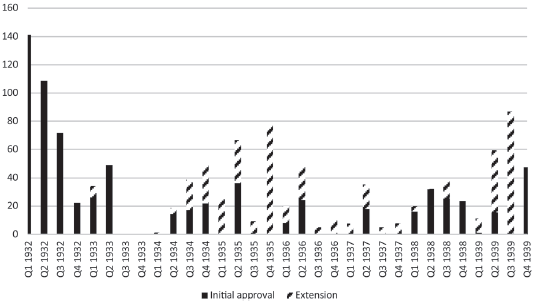
Although disclosure of RFC loans to banks was very sporadic, the ICC had a policy of full and timely disclosure of railroad loans. All railroad loans were publicly disclosed at or near the time of loan application and approval. We show the distribution of railroad bailout loans over time in Figure 4. The biggest concentration of loans was in 1932 and early 1933, followed by another wave of new loans and rollovers in 1935, and again in both 1938 and 1939.
RFC RAILROAD LOANS ($ MILLION, INCLUDING ROLLOVERS)
Notes: Value of approved bailouts for all class I railroads between 1932 and 1939 on a quarterly basis.
Sources: The New York Times and Final Report on the Reconstruction Finance Corporation.

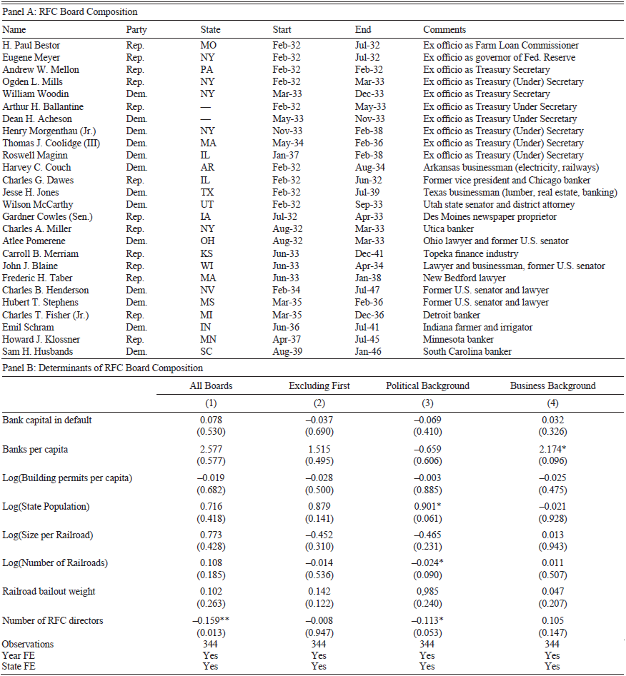
The RFC’s initial board of directors contained the Secretary of the Treasury, the Chairman of the Federal Reserve Board of Governors, and the Farm Loan Commissioner. The other directorships were balanced by party affiliation, and care was taken to ensure that the directors came from different regions of the United States. We read press reports, Final Report on the Reconstruction Finance Corporation (1959), and online biographies of the RFC directors to assign the directors’ “home” states. For example, The New York Times reported that two members of the initial RFC board would be “two Democrats from the Southwest, Harvey C. Couch of Arkansas and Jesse H. Jones of Texas.”Footnote 12 We document the composition of the RFC board in Table 1, Panel A. Most of the appointed RFC directors were businessmen, and four were former U.S. senators.
RFC BOARD COMPOSITION

* = Significant at the 10 percent level.
** = Significant at the 5 percent level.
*** = Significant at the 1 percent level.
Notes: Panel A reports the RFC board composition between 1932 and 1939. Party refers to the respective RFC director’s political party, where Dem. refers to Democrat and Rep. refers to Republican. State refers to the respective director’s home state. Start and End refer to the director’s start and end of service. Comments give insights into their background. In Panel B, the dependent variable equals one if an RFC director from state y was appointed to the board in year t, zero otherwise. Column (1) includes all state-years; Column (2) excludes appointments to the first board; Column (3) examines RFC directors with previous political experience; Column (4) examines RFC directors from the private sector. Bank Capital in Default is the ratio of national bank capital in default to total national bank capital in state y. Log(Size per Railroad) is the logarithm of the total assets of railroads active in state y divided by the number of railroads active in state y. Number of Railroads is the number of railroads active in state y. Railroad Bailout Weight is the ratio of the total assets of bailed-out railroads in year t active in state y to the total assets of railroads active in state y. Log(Building permits per capita) is the log of building permits divided by the state population in state y. Banks per capita is the number of national banks in state y divided by state population. Number of RFC directors is the number of existing RFC directors from state y. We cluster standard errors at the state level.
Source: Authors’ calculations
New Deal funding decisions are generally considered to have been at least partly politically motivated (see, e.g., Wright Reference Wright1974; Wallis Reference Wallis1987; Fishback, Kantor, and Wallis Reference Fishback, Kantor and Wallis2003). The RFC’s decisions were similarly criticized. In April 1932, Representative La Guardia claimed, “everybody in the country knows a private wire from J. P. Morgan to the headquarters in Washington dictates the [RFC’s] policy.”Footnote 13 The RFC’s initial president, former Vice President Charles G. Dawes, was heavily criticized by Senator Brookhart of Iowa for having loaned over $80 million to Dawes’ own Chicago bank.Footnote 14
Evidence of unethical practices in the granting of RFC railroad loans was also raised by the “Stock Exchange Practices” (known informally as the Pecora Report) investigation of the U.S. Senate Banking and Currency Committee. The final report stated that (p. 381) “J.P. Morgan & Co. … suggested that the (Missouri Pacific) railroad make application to the RFC to obtain the funds necessary to meet the bank loans of $11,700,00, although J.P. Morgan & Co. were conscious that the railroad was in a critical position, facing a public default.” J.P. Morgan & Co. had made loans to that railroad and was hoping to be repaid with the RFC money. Mason (Reference Mason2001) also mentions the existence of such incentives to borrow from the government to repay existing creditors.
Another troublesome connection (Part 8 of the Pecora Report, p. 4155) was that, “Mr (Harvey C.) Couch (RFC Board member, 1932–34) and I (Mr McCain, head of Chase National Bank) started out in the same small town in Arkansas 26 years ago, and we have been intimate and close friends ever since that time.” Couch and McCain’s “efforts have been principally in constructing the Louisiana and Arkansas (Railroad). We were interested in that because we came from Arkansas.” Louisiana and Arkansas were loaned $2.5 million by the RFC in 1940. Couch had been a director of the Chase National Bank before joining the RFC board. He admitted to McCain (p. 4168), “We (the RFC) finally made the Wabash (Railroad) loan after a lot of discussion.” The Chase National Bank had loaned the Wabash Railroad $3 million, and the bank was repaid following the granting of the RFC loan.
In our analysis, we demonstrate that RFC railroad loans were also partly determined by the geographical origins of the RFC board. We use the composition of the RFC board at the time loans were made as an instrument for loans. Board members were “known” to be associated with their home states (e.g., Harvey Couch). RFC applicants were also conscious of the board’s origins. Railroad magnate O.P. van Sweringen, who negotiated multiple RFC loans, testified that RFC board member Charles Miller (in part 2 of the Pecora hearings, p. 772), “is from New York State. He was not on (the RFC board) then but was afterwards, I believe … He is from New York State.”
The PWA also made government loans to railroads from late 1933 until early 1936. PWA loans tended to be smaller than the RFC’s disbursements, and they were often used for capital expenditure rather than to service the railroad’s debt. PWA loans comprise only around 10 percent of our sample by value and 15 percent of our sample by number. Since money is fungible (a railroad could apply to either government agency), we consider both RFC and PWA loans in our analysis.
Data
Data Sources
We study the Class I railroads of the continental United States. Class I railroads owned over 90 percent of the nation’s tracks by length, they employed roughly 98 percent of railroad employees (3.4 percent of the United States’ total labor force), and they carried over 99 percent of the revenue-ton-miles of all U.S. railroads in 1929. We collect balance sheets, profit and loss statements, track network data, and employment data from the annual reports of the ICC, Statistics of Railways in the United States. The number of railroads in our sample falls from 180 in 1929 to 144 in 1939, mostly due to acquisitions of struggling firms by stronger rivals.
We compile annual statistics for each railroad’s freight revenue sources (i.e., agricultural, animal, mining, forestry, merchandise, or manufacturing items) and monthly revenue from Moody’s Manual of Investments – Railroad Securities.
If a railroad had publicly traded equity, we gathered stock prices from the Center for Research in Security Prices (CRSP). Some railroads did not have publicly traded equity, usually because they were fully owned by another railway or a related industrial firm. We compiled price data on the most liquid railroad bonds.Footnote 15 We obtain bond prices from the section “Bond Sales on the New York Stock Exchange” in The New York Times. We classify a railroad as being in default if it has failed to meet a coupon or principal repayment or if it in any way changed the terms of the issue.Footnote 16 Data on bond ratings, coupons, amounts outstanding, and maturity come from Moody’s. We use Moody’s index of daily railroad bond prices, reported in the Commercial & Financial Chronicle, as a proxy for the market return on railroad bonds.
We combine the track network of each railroad with a city-level data source. We hand-collect data on factories operated by New York Stock Exchange (NYSE)-listed manufacturing firms from Moody’s Manual of Investments – Industrial Securities. There are 471 manufacturing firms with data on factories reported in Moody’s. We collect national bank capital in default from the Annual Report of the Comptroller of the Currency. National bank capital per state comes from Flood (Reference Flood1998).
Bailouts
We identify railroad bailouts from the RFC’s records at the National Archives in Washington.Footnote 17 For each railroad, we observe their application, approval, and refusal documents, along with the dates on which each document was sent. Loan decisions were made quickly, usually taking a couple of weeks to a month or two. The median (mean) time for a decision to be made was 27 (45) days.
To identify the public announcement date of railroad bailouts, we search The New York Times for the phrases “Reconstruction Finance Corporation” or “Public Works Administration” from January 1932 until December 1939. We identify loan applications, approvals, rejections, and details thereof in the archives. 89.5 percent of all applications, approvals, and refusals from the archives also appear in The New York Times.
Occasionally, a railroad would revise the size of its loan request while the application was under consideration. For example, the RFC might agree to loan a railroad a smaller amount than initially requested and would invite the railroad to modify its application. Alternatively, a railroad might have been successful in obtaining some funds from other sources and reduced its loan request.
Results
RFC Board Composition
Our analysis uses the dataset of Verdickt and Moore (2025).
In Table 1, Panel A, we present data on RFC directors. The composition was supposed to be balanced by party affiliation and geographically diverse. However, it is possible that the appointment of RFC directors was partly determined by economic conditions in the home state of the director or even by financial conditions in the railway sector in their home states.
In Panel B, we run the following regression to better understand the relationship between economic conditions and RFC directors:
where RFC t+1,i is defined as the number of RFC directors in state i at time t+1, Xt,i is a vector of state characteristics at time t, and we include year (θ t) and state (πs), fixed effects.
We documented that states with a faster-growing population were more likely to have RFC directors, and directors were less likely to be appointed if there was already an existing director from the same state. Our results show that the appointment of directors is not robustly associated with economic conditions in the directors’ home states. Therefore, concerns are alleviated that causality runs from the poor economic conditions of railroads to the appointment of RFC directors and thence to more railroad bailouts.
Summary Statistics
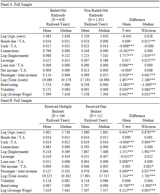
In Table 2, we present summary statistics on railroads. We divide railroads into those that were “bailed-out”—those that received at least one loan from the RFC or the PWA between 1932 and 1939—and those that were not bailed-out. In Panel A, we show that there are large differences between the bailout recipients and others. Bailed-out railroads had less cash to total assets (a mean of 1.5 percent of assets vs. 2.3 percent for non-bailed-out railroads), were slightly more leveraged (mean long-term debt to total assets of 42.5 percent vs. 40.7 percent), and had more bonds maturing in the depths of the Depression. They were also less profitable (a mean net income to total assets of 0.9 percent vs. 1.3 percent) and had more volatile operations (monthly volatility of 12.3 percent vs. 9.2 percent). Bailed-out railroads were much larger (mean total assets of $195.1 million vs. $29.2 million), employed more people (a median of 9,145 vs. 1,214), had higher average wages ($1,634 vs. $1,568), and had more connections to the RFC board. Connections are the number of states in which the railroad operated that were homes to RFC directors that year. On average, bailed-out railroads operated in 0.8 states with an RFC director vs. 0.4 states for non-bailed-out railroads.Footnote 18
RAILROAD SUMMARY STATISTICS

* = Significant at the 10 percent level.
** = Significant at the 5 percent level.
*** = Significant at the 1 percent level.
Notes: The sample consists of 2,590 annual observations for 183 railroads from 1927 to 1939. A bailout is defined as any loan from the Reconstruction Finance Corporation (RFC) or Public Works Administration (PWA) from 1932 to 1939. Connections is the number of states the railroad operated in that were home to RFC directors in that year. Leverage is the ratio of long-term debt to total assets. Bonds Due / T.A. is the value of all bonds due between 1930 and 1934 to total assets in 1929. Passenger / Total Revenue equals passenger revenue divided by total revenue. Bond Rating is the average Moody’s rating of the railroads’ listed bonds (9=Aaa, 8= Aa, etc.) Volatility is the standard deviation of the previous 12 months’ earnings (if earnings were missing, the 12-month standard deviation of stock returns). Average Wage is the total expense on employees divided by the number of employees. We report tests of differences in means (t-test) and medians (Wilcoxon) between the groups.
Source: See the text.
In Panel B, we subdivide the bailed-out railroads into two groups: those that received a single loan from the RFC or PWA and those that received multiple bailouts between 1932 and 1939. The railroads that received multiple bailouts tended to have less cash (mean 1.4 percent of total assets vs. 1.9 percent) and were better connected to the RFC (connections in 0.9 states vs. 0.4 states). The companies that obtained multiple bailouts tended to be larger (mean size of $247.0 million vs. $65.1 million), employed more people (a mean of 10,076 people vs. 2,609 people), and focused more on passengers (12.5 percent vs. 7.6 percent of total revenue at the mean).
Bailout Recipients
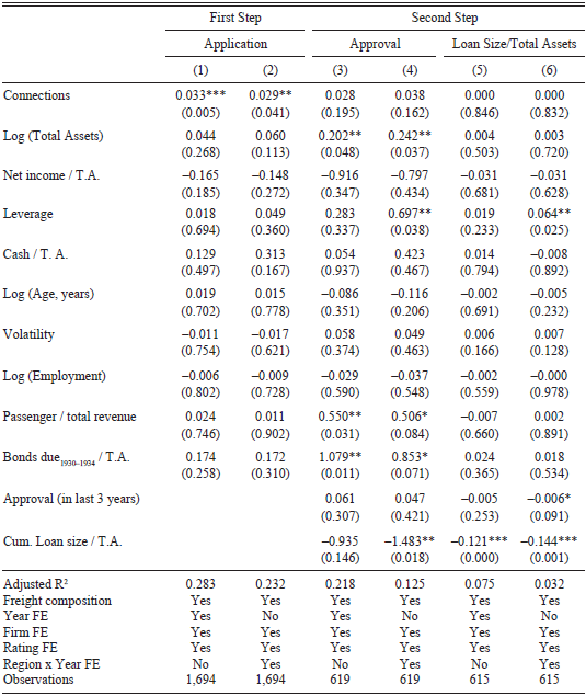
We use a two-step model to investigate which railroads received the government bailouts, in the spirit of Vossmeyer (Reference Vossmeyer2016). In the first step, we run an OLS model of railroads’ applications on their lagged characteristics:
where Application t+1,i equals one if firm i applied for (at least) one bailout in year t+1, and zero otherwise, Connections t,i is the number of political connections for firm i at time t, X t,i is a vector of firm characteristics at time t, and we include the year (θ t), bond rating (π t,i), and region-year (φ r,t) fixed effects.
In Column (1) of Table 3, we show that railroads were more likely to apply for a bailout when they had more connections to the RFC. An increase in the number of connections of one leads to an increase in the probability of applying by 0.033 (significant at the 1 percent confidence level). Given that the average probability of applying equals 0.067, this effect is economically large. Railroad financial strength, such as cash holdings, leverage, and profitability does not change the likelihood of a railroad applying for a bailout, although larger railroads were more likely to apply.Footnote 19 In Column (2), we show that allowing for unobserved, time-varying shocks at the regional level does not change our results.
DETERMINANTS OF BAILOUT

* = Significant at the 10 percent level.
** = Significant at the 5 percent level.
*** = Significant at the 1 percent level.
Notes: We regress bailouts on railroad characteristics in a two-step regression. In Step 1, (Columns (1) and (2)) we regress Application (equal to one if the railroad applied for at least one loan in that year, and zero otherwise) on railroad characteristics. In Step 2, we exclude railroads that did not apply for a bailout in that year. Columns (3) and (4) present a regression where the dependent variable, Approval, equals one if the railroad was approved for at least one loan in that year, and zero otherwise. Columns (5) and (6) present a regression in which the dependent variable is the railroad’s loan size divided by total assets. Approval (in last 3 Years) is a dummy variable that equals one if the railroad had an RFC or PWA loan approved in the last three years, and zero otherwise. Cum. Loan Size / T.A. equals the cumulative loan amounts a railroad has received since 1932 divided by its total assets. Other variables are defined in Table 2.
Source: See the text.
In the second step, we study which characteristics correlate with a loan approval, among railroads that applied for loans in that year:
where X t+1,i equals one if firm i received at least one bailout in year t+1 (Columns (3) and (4)), or size of loan approvals scaled by total assets (Columns (5) and (6)), and zero otherwise, Connections t,i is the number of political connections for firm i at time t, X t,i is a vector of firm characteristics at time t, and we add year (θ t), bond rating (π t,i), and region-year (φ r,t) fixed effects.
In Columns (3) and (4), we find that successful applicants were, on average, larger, more leveraged, focused more on passengers, and had more bonds that were close to maturity.Footnote 20 Applicants who had received more loans in the past were less likely to be approved. When we take the unobserved, time-varying regional effects into account (Column (4)), we see little change.
In Columns (5) and (6), we examine the size of loan approvals (scaled by total assets). We see that more leveraged railroads tended to receive larger loans, and applicants who had received more prior loans from the government tended to receive smaller loans. Railroads whose leverage was one standard deviation higher (15.9 percentage points of total assets) received a bailout that was, on average, 38.9 percent higher.
Although having a connection to the RFC was important in generating railroad loan applications (Columns (1) and (2)), connections to the RFC board did not appear to increase the likelihood of loan approval or loan size (Columns (3)–(6)). Since ICC and RFC approval were required before a loan could be granted, our results may shed light on the political process. One reason why RFC board links to railroads may not have been important is that the RFC chairman from 1933 to 1939, Jesse Jones, claimed, “I assumed personal charge of practically all negotiations in the railroad field” (1951, p. 106).Footnote 21 Railroads with connections to the RFC board may have believed that they would be favorably treated in the loan process; hence, they submitted more applications. However, the ICC may have acted as a check on such favoritism, which eliminated the possibility of favorable treatment in the loan approval process. In unreported results, we find that connections between an investment bank (J.P. Morgan & Co., Kuhn, Loeb & Co., or Dillon, Read & Co.) and a railroad, as documented in the Pecora Report, slightly increased the chance that the railroad would apply for a government loan and be approved for that loan. Conditional on investment bank links, railroads with connections to the RFC board were slightly more likely to be approved for government loans.Footnote 22
Market Reactions to Bailouts
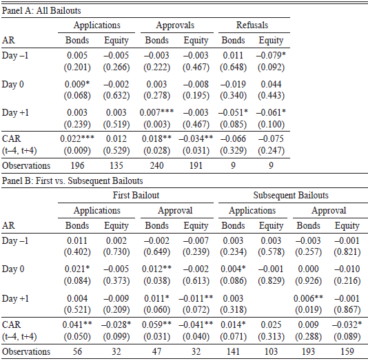
We examine the reactions of a railroad’s stock and bond prices to The New York Times’ reports of bailout applications and approvals. In Table 4, we compute abnormal returns and cumulative abnormal returns (CAR) on railroad debt and equity. We compute AR as the return on the stock or the bond minus an equally-weighted railroad equity index (from CRSP data) or Moody’s railroad bond index return, respectively.
where R t,i,p is the return at time t for firm i for security p (either stocks or bonds), and RM t,o,p is the market return at time t for index o for security p.
ANNOUNCEMENT EFFECTS

* = Significant at the 10 percent level.
** = Significant at the 5 percent level.
*** = Significant at the 1 percent level.
Notes: We calculate the abnormal returns (AR) and cumulative abnormal returns (CAR) of a security from four days before to four days after the announcement of an application, approval, or refusal. We measure the AR as the bond’s (equity’s) return minus the Moody’s bond index (equally-weighted CRSP railroad equity index) on the same day. We average the AR (CAR) across securities. Standard errors are clustered by railroads. p-values appear in parentheses. Panel A presents the results for all bailouts. Panel B presents the results for the initial and subsequent bailouts.
Source: See the text.
We find a statistically significant AR of 0.9 percent for bonds on the day a loan application was announced and a statistically insignificant abnormal return of 0.3 percent on the day an approval was announced (see Panel A). In the window around the news release (t–4 to t+4), we find bond CARs of 2.2 percent (applications), 1.8 percent (approvals), and –6.6 percent (refusals).
Since many railroads applied for (and were granted) multiple loans, we investigate the differences between the initial loan and subsequent loans. Substantially more information is likely to have been conveyed to the market by a firm’s initial revelation that it desired federal government financial assistance than by follow-up applications. An application for the first bailout is associated with a 4.1 percent bond CAR from t–4 to t+4, and a 2.1 percent AR on day zero (see Panel B). An approval announcement for the first bailout has a 1.2 percent bond AR on day zero (with a 5.9 percent CAR from t–4 to t+4), all statistically significant. Subsequent bailouts are reflected in more subdued bond responses. The bond CAR for subsequent application announcements equals 1.4 percent from day t–4 to t+4 (statistically significant), while subsequent approvals are a statistically insignificant at 0.9 percent. There is also a statistically significant movement of stock prices in response to bailout news. An approval announcement coincides with a statistically significant –3.4 percent equity CAR (from t–4 to t+4). This effect is similar for both the first and subsequent bailouts. The small positive response of bond prices to RFC loan news needs to be placed in a context in which railroad bonds had dropped dramatically in price (Figure 3).
The favorable response of bond prices to loan applications and approvals indicates that a government bailout was a positive sign for bondholders. Government funds were provided at below-market rates to railroads that were having difficulty borrowing in the private sector. A loan could also help the company to survive for longer. However, if the railroad were required to restructure or file for bankruptcy in the future, existing shareholders would become more junior (to the government) claimants on the railroad’s assets (see Mason and Schiffman Reference Mason, Schiffman and Gup2004, pp. 56–7), which was unfavorable news for shareholders.
Effectiveness of Government Bailouts
We now examine if railroad bailouts achieved the RFC’s twin objectives. We first investigate whether the bailouts helped railroads avoid defaulting on their bonds. Second, we look at how the bailouts affected railroad employment, wages, and operating performance. Finally, we search for evidence that bailouts provided positive spillovers for firms located near the bailed-out railroads.
Credit Structure
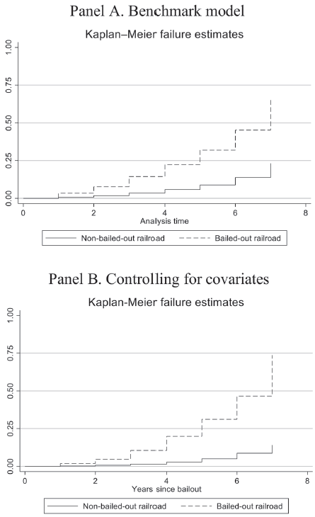
Did the RFC protect the “credit structure” of the financial system? All else equal, an RFC loan should have made a railroad less likely to default on its debt. Jones (Reference Jones1951) claims that RFC funding reduced railroad defaults by half, whereas Schiffman (Reference Schiffman2003) and Mason and Schiffman (Reference Mason, Schiffman and Gup2004) claim that bailouts at least delayed defaults.Footnote 23 However, defaulting on debt is partly a choice, and Mason and Schiffman argue that bankruptcy, “brought relief from high fixed charges that were often a principal cause of financial distress” (p. 61). In Figure 5, we plot Kaplan-Meier (Reference Kaplan and Meier1958) graphs with cumulative probabilities of failure for the bailed-out vs. non-bailed-out railroads. We observe that railroads that received a bailout are associated with a higher hazard rate of bond defaults, that this difference increases with time from the bailout, and that including observable control variables does not alter the result. The granting of a below-market-rate loan, ceteris paribus, is a good event. Hence, higher default rates for bailed-out railroads suggest that unobservable factors are likely influencing both a railroad’s performance and the bailout decision.
KAPLAN-MEIER FAILURE GRAPHS
Notes: Hazard rates of bond defaults in the years after a bailout. Panel A compares bailed-out to non-bailed-out railroads. Panel B shows hazard rates after controlling for lagged railroad characteristics, such as (log) total assets, net income to total assets, cash to total assets, leverage, (log) employment, (log) firm age, bonds due between 1930 and 1934 to total assets, passenger revenue to total revenue, and the freight composition.
Source: See the text.

We investigate defaults with the following regression:
where Default t+1→t+3,i is an indicator variable measuring a bond default for firm i between time t and time t+1 (or t+3), Connections t,i is the number of political connections for firm i at time t, X t,i is a vector of firm characteristics at time t, and we include year (θ t), bond rating (π t,i), and region (φ r) fixed effects.
We assess the effects of bailouts on bond defaults in Table 5. In Column (1), we run a probit model in which the dependent variable equals one if a railroad defaulted on its bonds in that year. We examine whether loan Approval in the previous year is associated with the railroad defaulting on its debt. We attempt to capture railroad unobservables by including bond rating fixed effects from Moody’s. Lower net income, lower cash to assets, and younger railroads are associated with a higher likelihood of default. Government loan Approval does not have a statistically significant relation with defaults.
DETERMINANTS OF BOND DEFAULTS

* = Significant at the 10 percent level.
** = Significant at the 5 percent level.
*** = Significant at the 1 percent level.
Notes: We regress bond defaults on lagged railroad characteristics. Default equals one if the railroad failed to meet a coupon or principal repayment, or in any way changed the terms of the issue in the current year. We drop all observations of a railroad the year after it defaults. Approval equals one if the railroad obtained an RFC or PWA loan in the previous year. Columns (1) and (4) contain probit results. In Columns (2) and (5), we present our first-stage regression for the instrumental-variable (IV) approach. We regress an indicator variable equal to one in the year the railroad received an Approval, and zero otherwise, on railroad controls. In Columns (3) and (6), we present the second-stage instrumental variable (IV) regression. p-values, in parentheses, are adjusted for heteroskedasticity and clustered at the railroad-level. We include region, year and bond rating fixed effects. For a railroad with multiple outstanding bonds, we use the rating of the bond closest to maturity.
Source: See the text.
In Column (4), we again run a probit model of defaults, but the dependent variable now equals one if a railroad defaulted in that year or in the following two years. This offers a longer-run investigation of how a government loan Approval is associated with a railroad’s likelihood of default. We find that Approval has a significantly positive correlation with the probability of railroad default (at the 5 percent confidence level). An RFC or PWA bailout is associated with a default rate of 6.39 percent, all other characteristics at sample means, relative to a non-bailed-out railroad’s default rate of 1.51 percent. However, railroad bailouts are unlikely to be awarded at random, and a selection effect is likely to be present. Hence, we turn to an instrumental variable approach to determine whether bailouts have a causal effect on railroad defaults.
Instrumenting for Bailouts
Our concern in determining if bailouts aided railroads is that there are likely to be variables omitted from our econometric specification that partly affected a railroad’s default behavior. Railroad management and the RFC board had access to non-public information and may have used such information in the decision to grant or deny a government loan. The RFC required all railroads that applied for loans to disclose the “possibility of securing a loan from other sources” (item 3 of the application). For example, the Chicago and NorthWestern Railroad, in applying for $11,127,700 on 16 January 1933, reported to the RFC that “for many years Applicant ordinarily has been financed through Kuhn, Loeb and Company, Investment Brokers of New York City … on different occasions during the latter part of 1932 Applicant discussed … the possibility of securing a loan … but Kuhn, Loeb and Company declined to commit itself to any future loans.” A railroad that had tried, but failed, to obtain bank or Wall Street loans would be more likely to default than its observable characteristics would suggest. In such a situation, the error from the regression of bond defaults on bailouts is likely to be correlated with the independent variable Approval if the RFC was at least partly conditioning government loan approval on a railroad’s current and future situation. Therefore, the coefficient estimates on Approval, which measure the effectiveness of government aid, will be biased.
It is a priori unclear in which direction the bias will lie. One of the RFC’s objectives was to stimulate employment; therefore, loans may have been granted to railroads in worse shape than their observables would suggest, in an attempt to forestall a debt default and subsequent layoffs of employees. Political interference in the loan process may also have led to loans being granted to railroads in more perilous shape than it appeared on the surface. On the other hand, the RFC was only supposed to make loans that were “adequately secured” by collateral. The requirements for good quality collateral may have led to loans being directed toward railroads that were in better shape than their observable characteristics indicated. The existence of bias is not certain. Spero (Reference Spero1939, p. 2) claims that, “initially the [RFC] was … paying little heed to the financial position and structure of the applicants and their earnings potentiality,” which discounts the possibility of non-public information usage in evaluating loans, at least near the start of our sample.
We want an instrumental variable that is correlated with a railroad receiving a government bailout but only affects a railroad’s financial performance through the granting of RFC loans. We take advantage of the prior literature that claims New Deal grants were influenced by politics. Fishback (Reference Fishback2017, p. 1444), for example, concludes, “nearly every study finds that political considerations were important to the Roosevelt administration.” There are, however, some investigations of New Deal funding, such as Mason (Reference Mason2003), that find little political influence. We use the composition of the RFC board as our instrumental variable. Specifically, we use the number of states a railroad passed through that were the home states of RFC directors in that particular year. We call this the number of a railroad’s Connections to the RFC. For example, on 5 February 1932, the Chicago and Eastern Illinois railroad applied for an RFC loan for $3.629 million. This railroad passed through Illinois, Indiana, and Missouri. H. Paul Bestor (Missouri) and Charles G. Dawes (Illinois) sat on the board of the RFC at the time of the application. Therefore, our instrument takes a value of two.
In our first-stage regression (Table 5, Columns (2) and (5)), we regress Approval on a railroad’s lagged characteristics and our instrument, Connections. We see that Approval is positively and statistically significantly related to a railroad’s Connections, even with region, year, and bond-rating fixed effects. The F-statistic in the first-stage regression is 36.37, which indicates that we have a strong instrument.
To have a valid instrument, we also require that the exclusion restriction is satisfied. The exclusion restriction requires that Connections are uncorrelated with the error term, the unobservable part of a railroad’s financial position that partly determines default behavior. There was no realistic possibility that a railroad that was doing poorly, based on unobservable factors, could quickly change its number of Connections by altering its operations. It would be expensive and take years of construction for an existing railroad to begin operations in the home state of an RFC director.
It would also invalidate our instrument if railroads that were in worse financial shape than their observable characteristics suggested were able to influence the president to alter the RFC board’s composition, such that a new director was appointed from a state in which the railroad operated. RFC directors were responsible for approving all loans that the Corporation made, railroad and non-railroad alike. Total railroad loans comprised a fraction of the RFC’s disbursements, and loans to an individual railroad were a tiny percentage of total RFC expenditure. There were only five to seven directors at any one time, and the composition was balanced by political affiliation and by the need to have directors come from different parts of the country. Given these constraints on the composition of the RFC board, we believe it is extremely unlikely that certain railroads could have increased their Connections by lobbying.
In Columns (3) and (6) of Table 5, we replace Approval with its predicted level from the first-stage regression. We see that bailouts do not have a statistically significant relation with a railroad’s defaults. Our point estimates indicate loan approvals reduce defaults in the subsequent year (Column (3)), in line with Spero’s (Reference Spero1939) claim that bailouts, “merely preserved, for a time, unsound, fair-weather financial structures” (p. 141). Our point estimate is that a bailout increased defaults in the longer term (Column (6)). Overall, government aid did not seem to aid railroads avoiding default for very long.
Operating Performance, Instrumental Variables
In Table 6, we again make use of the board composition of the RFC and our measure, Connections, as an instrument for railroad bailouts. In the second stage, we regress railroad leverage, employment, wages, and profitability on the fitted level of bailouts after conditioning on railroad characteristics:
where Y t+1,i is the employment, leverage, average wage, or profitability for firm i at time t+1, Connections t,i is the number of political connections for firm i at time t, X t,i is a vector of firm characteristics at time t, and we include year (θ t), bond rating (π t,i), and region (φ r) fixed effects.
INSTRUMENTAL VARIABLE REGRESSIONS: LEVERAGE, EMPLOYMENT, WAGES, AND PROFITABILITY

* = Significant at the 10 percent level.
** = Significant at the 5 percent level.
*** = Significant at the 1 percent level.
Notes: In the first stage, we regress Approval on Connections and lagged railroad characteristics. In the second stage, we regress contemporaneous railroad leverage, log(employment), log(average wage), and profitability on the fitted level of lagged Approval and lagged characteristics. Variables are as defined in Tables 2 and 3. p-values are adjusted for heteroskedasticity and clustered at the firm-level, in parentheses.
Source: See the text.
We find that a bailout causes a 10.2 percentage point decrease in leverage (Column (2)). We find no statistically significant impact of bailouts on employment (Column (3)) or profitability (Column (5)). However, there was an increase of 15.4 percentage points in the average wage (Column (4)). Therefore, we conclude that the RFC failed in its second objective, which was to promote railroad employment. Schiffman (Reference Schiffman2003, p. 821) also finds that, “RFC loans had no positive impact on … employment.” All regressions use firm, year, and region fixed effects and condition on lagged characteristics. Railroads appear to have used bailouts to reduce their leverage and increase wages, with little beneficial impact on employment.
As the RFC’s largest volume of loans was made in 1932 during the depths of the Depression (see Figure 4), and the lending criteria were tightened in mid-1933, the earlier loans may differ in their effects from the later loans. We redo the analysis of Table 6 with a subsample of pre-June 1933 RFC loans. In that analysis, we find no statistically significant effect of government loans on leverage, employment, wages, or profitability.
Interpretation of Instrumental Variable Effects
Our approach estimates the local average treatment effect (see Imbens and Angrist (Reference Imbens and Angrist1994)). In our setting, we estimate the effect of an RFC bailout on railroads whose treatment (a bailout or not) can be affected by the instrument (a connected board of directors). U.S. railroads can be thought of as comprising three sub-groups: “compliers”—railroads who would receive a loan if they had a connected board, but no loan without such a connection; “always takers”—railroads who would receive a loan, due to their financial status or economic importance, no matter the composition of their board; and “never takers”—railroads who would never receive an RFC loan, due to their financial situation or economic importance. Our instrumental variables approach can only measure the treatment effect on the “compliers” group (see Angrist and Pischke Reference Angrist and Pischke2009, p. 160). The treatment effect of the RFC program on “always takers” and “never takers” cannot be inferred from our approach without making further assumptions. Therefore, the RFC’s bailout program may have had a larger or smaller impact on the railroad industry outcomes than our estimates suggest.
Economic Spillovers
Bailouts do not seem to have provided many direct benefits for the recipients—save a jump in the price of their bonds. They may, however, have provided spillover benefits for firms located close to the railroad. For example, a railroad bailout may have helped it to keep operating routes that would otherwise have been closed or to conduct a more frequent schedule.
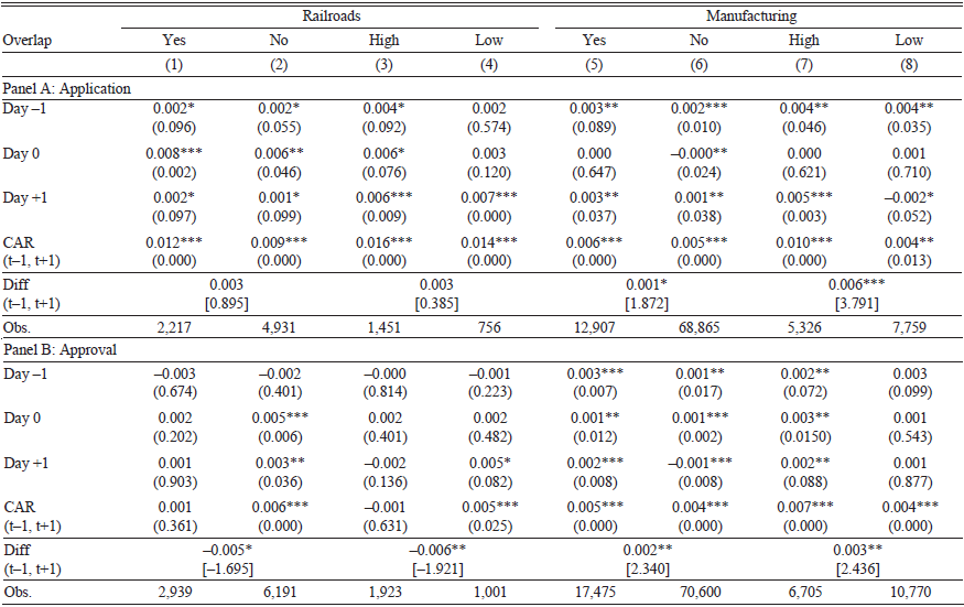
In Table 7, we study whether news of a railroad’s bailout affected other railroads and manufacturing firms listed on the NYSE. If a bailout was “good news,” we might expect local manufacturing businesses to respond positively to news of a bailout. We interpret the change in local businesses’ stock prices upon news of a railroad bailout as an indicator of whether local businesses were expected to benefit or be harmed by a railroad bailout. We calculate the AR and CAR of firms’ equity and focus on the interesting cross-sectional evidence: which manufacturing firms and which railroads benefited most from news of one railroad’s bailout?
ANNOUNCEMENT EFFECTS FOR RELATED FIRMS

* = Significant at the 10 percent level.
** = Significant at the 5 percent level.
*** = Significant at the 1 percent level.
Notes: We calculate the abnormal return (AR) and cumulative abnormal return (CAR) for related firms’ equity after the announcement of a railroad’s bailout application (Panel A) and approval (Panel B). We measure the AR as the firm’s equity return minus a CRSP equally-weighted railroad/manufacturing index. An overlap of Yes indicates the railroad/manufacturing firm operates in at least one city with the bailed-out railroad. An overlap of No indicates the railroad/manufacturing firm does not operate in any cities in which the bailed-out railroad operates. High indicates that the percentage overlap is above the mean level across all firms. Low indicates that the percentage overlap is non-zero and below the mean overlap across all firms. For railroads, the percentage overlap is defined as the number of cities that both railroads serve divided by the total number of cities of the bailed-out railroad. For manufacturing firms, the percentage overlap is defined as the number of cities the railroad and manufacturing firm operate in divided by the total number of cities the manufacturer operates in. p-values appear in parentheses. We report the p-values of t-test differences between the groups (Yes – No or High – Low) in Diff. The returns are winsorized at the 2.5 percent level.
Source: See the text.
We cross-sectionally split firms along two dimensions. First, did the other railroad overlap with the bailed-out railroad at all, meaning did both railroads service at least one common city (Yes or No)? Second, was the level of overlap (the fraction of the bailed-out railroad’s cities also serviced by the other railroad) above the sample mean (High), or was the overlap positive but below the sample mean (Low)? We construct similar overlap measures for manufacturing firms, but we consider the joint presence of manufacturing establishments and railroad tracks.
In Panel A, we see that there was no statistical difference between the mean CARs of railroads that overlapped with the bailed-out railroad and non-overlapping railroads upon news of an RFC application. Nor was there a statistically significant difference between high overlap railroads and low overlap railroads. In Panel B, we observe slightly smaller, –0.5 percent (Yes less No) to –0.6 percent (High less Low), and statistically significant differences in CARs for other railroads upon RFC approvals. We interpret this result to mean that competing railroads (i.e., those with some overlap with the bailout recipient) suffered slightly from government assistance to a rival, relative to railroads that had little or no overlap. As this is a cross-sectional test, we are conditioning on any economy-wide railroad shocks, such as changes in government railroad policy, input costs, or demand changes.
We also compare manufacturing firms that were co-located in the same city as the bailed-out railroad (an overlap of Yes or High) to manufacturing firms that were not (or not mainly) located in cities through which the bailed-out railroad ran (No or Low). We see that a railroad bailout benefited co-located manufacturers relative to manufacturers that were not located near the bailout recipient’s tracks. Co-located manufacturing firms outperformed others by 0.1 percent (Yes vs. No) at the time of the application and 0.2 percent at the time of the approval. If we compare High vs. Low manufacturing firms, we see that high overlap manufacturers outperformed by 0.6 percent at the time of application (Panel A) and 0.3 percent at the time of approval (Panel B). Taken together, there is modest evidence that railroad bailouts provided positive economic spillovers to the real economy, even if the railroads themselves showed little direct benefit from the bailout. However, it needs to be kept in mind that measuring the state of the economy by the stock price movements of local businesses that were listed on the NYSE is necessarily imprecise. The suggestive evidence we present of economic spillovers is far from definitive.
Conclusion
The RFC distributed much of the U.S. government’s New Deal assistance to the economy as it struggled with the Great Depression. Around 10 percent of the RFC’s loans were given to railroads, along with limited assistance from the PWA. In our study, we ask if such bailouts aided railroads in avoiding debt defaults and stimulating employment, which were the RFC’s twin objectives.
First, using an instrumental variables approach, we find scant evidence that government assistance increased railroad employment, although it led to an increase in wages for existing employees. Second, while bond markets reacted positively to both the creation of the RFC and loan announcements—suggesting markets viewed government support as valuable—we do not find evidence that the actual distribution of government aid prevented bond defaults for specific railroads. The bailouts did help to reduce leverage, reflected in both balance sheet improvements and positive bond price reactions around loan announcements and approvals.
Overall, our evidence suggests the program’s benefits flowed primarily to existing employees through higher wages—and bondholders—through reduced leverage and positive price reactions—rather than improving broader measures of firm performance, such as employment or profitability.
Non-bailed-out railroads that competed with the recipient seem to have suffered some harm from the bailout, presumably because one of their competitors was supported financially. We find evidence that government railroad support was beneficial for manufacturing firms that were co-located near the railroad’s tracks. As such, although RFC and PWA assistance proved of little benefit to the railroad itself, we find positive economic spillovers to manufacturers from this New Deal program.


 Open access